1 Introduction
We consider the global-in-time existence and singularity formation of radially symmetric relativistic smooth flows. The system of equations for the relativistic fluid dynamics, as an important representative model of nonlinear hyperbolic conservation laws, has wide applications in several fields, such as astrophysics, plasma physics, and nuclear physics, and has been extensively studied by many mathematicians and physicists. The motion of perfect inviscid fluids in the
 $(d+1)$
-dimensional Minkowski space-time
 $(t,x)\in \mathbb {R}_+\times \mathbb {R}^d\ (d\geq 1)$
in special relativity can be described by the isentropic relativistic Euler equations (e.g., [Reference Chen15, Reference Pan and Smoller48, Reference Pant50, Reference Smoller and Temple53])
 $$ \begin{align} \left\{ \begin{array}{l} \displaystyle \bigg(\frac{\rho+\varepsilon p}{1-\varepsilon \textbf{u}^2}-\varepsilon p\bigg)_t +\nabla\cdot\bigg(\frac{\rho+\varepsilon p}{1-\varepsilon \textbf{u}^2}\textbf{u}\bigg)=0, \\[10pt] \displaystyle \bigg(\frac{\rho+\varepsilon p}{1-\varepsilon \textbf{u}^2}\textbf{u}\bigg)_t +\nabla\cdot\bigg(\frac{\rho+\varepsilon p}{1-\varepsilon \textbf{u}^2}\textbf{u}\otimes \textbf{u}+p\bigg)=0, \end{array} \right. \end{align} $$
where
 $\rho $
is the mass–energy density of fluid,
 $p=p(\rho )$
is the pressure,
 $\textbf {u}=(u_1,\ldots ,u_d)$
is the particle speed,
 $\varepsilon =1/c^2$
, and
 $c>0$
is the light speed. The first and second equations in (1.1) are the conservation laws in energy and momentum for the relativistic fluids. We are interested in system (1.1) with the classical equation of state for the polytropic ideal gas
 $$ \begin{align} p(\rho)=A\rho^{\gamma}, \end{align} $$
where A is a positive constant and
 $\gamma>1$
is the adiabatic constant. The relativistic constraint leads to the corresponding physical area
 $$ \begin{align*} \Pi=\Big\{(\rho, \textbf{u})|\ 0\leq \rho<\rho^{*}; |\textbf{u}|=\sqrt{u_1^2+\cdots+u_d^2}<\frac{1}{\sqrt{\varepsilon}} \Big\}, \end{align*} $$
where the number
 $\rho ^{*}$
is determined by
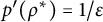 $p'(\rho ^*)=1/\varepsilon $
.
For a radially symmetric relativistic flow, that is, the solution has the following geometric structure:
 $$ \begin{align} \begin{aligned}\rho(\textbf{x},t)=\rho(r,t), \quad u_i(\textbf{x},t)=\frac{x_i}{r}u(r,t), \\ r=|\textbf{x}|=\sqrt{x_{1}^2+\cdots+x_{d}^2}\quad \text{with}\quad d>1, \end{aligned}\end{align} $$
where
 $u(r,t)$
is a scalar function, system (1.1) can be reduced to
 $$ \begin{align} \left\{ \begin{array}{ll} \displaystyle \bigg(\frac{\rho+\varepsilon p}{1-\varepsilon u^2}-\varepsilon p\bigg)_t +\bigg(\frac{\rho+\varepsilon p}{1-\varepsilon u^2}u\bigg)_r=-\frac{(d-1)(\rho+\varepsilon p)u}{r(1-\varepsilon u^2)}, \\[10pt] \displaystyle \bigg(\frac{\rho+\varepsilon p}{1-\varepsilon u^2}u\bigg)_t +\bigg(\frac{\rho+\varepsilon p}{1-\varepsilon u^2}u^2+p\bigg)_r=-\frac{(d-1)(\rho+\varepsilon p)u^2}{r(1-\varepsilon u^2)}. \end{array} \right. \end{align} $$
In this article, we tackle the problems of global existence and singularity formation of smooth solutions to system (1.4) in all dimensions
 $d>1$
. Particularity, system (1.4) with
 $d=2$
and
 $d=3$
correspond to the cylindrically and spherically symmetric relativistic Euler equations, respectively. In the Newtonian limit (
 $c\rightarrow \infty $
), system (1.4) formally reduces to the classical radially symmetric isentropic Euler equations
 $$ \begin{align} \left\{ \begin{array}{l} \displaystyle \rho_t+(\rho u)_r=-\frac{(d-1)\rho u}{r}, \\ [6pt] \displaystyle (\rho u)_t+(\rho u^2+p)_r=-\frac{(d-1)\rho u^2}{r}. \end{array} \right. \end{align} $$
Many excellent pieces of work have been contributed on the study of one-dimensional isentropic relativistic Euler equations (1.1) with the equation of state (1.2). We refer the reader to, e.g., works on the Riemann solutions [Reference Chen and Li13, Reference Chen15], on the local existence of smooth solutions [Reference Geng and Li21, Reference Makino and Ukai47], on the formation of singularities of smooth solutions [Reference Athanasiou, Bayles-Rea and Zhu1, Reference Athanasiou and Zhu2, Reference Guo and Tahvildar-Zedeh24, Reference Pan and Smoller48] and on the studies of weak solutions [Reference Chen and Schrecker14, Reference Frid and Perepelitsa20, Reference Hsu, Lin and Makino30, Reference Li and Shi43, Reference Pant50, Reference Smoller and Temple53]. In [Reference Ruan and Zhu51], Ruan and Zhu established an existence theorem of global smooth solutions to its Cauchy problem by applying the characteristic method and maximum principle. The global existence of smooth solutions for some general one-dimensional quasilinear hyperbolic systems was presented in [Reference Li40, Reference Li, Zhou and Kong42].
As a special but physically interesting multi-dimensional flow, the radially symmetric relativistic Euler equations (1.4) has also been broadly investigated. By using Sideris’s framework [Reference Sideris52], singularity formation results of smooth solutions to the multi-dimensional relativistic Euler equations with polytropic gases were presented in [Reference Athanasiou and Zhu2, Reference Guo and Tahvildar-Zedeh24, Reference Pan and Smoller48, Reference Wei54]. The framework of Sideris is based on the establishment of differential inequalities for some averaged quantities, and therefore cannot provide a local analysis of the singularity. For more general solutions in multiple space dimensions, a geometric framework was introduced by Christodoulou [Reference Christodoulou16] to study the singularity formation of smooth solutions for the relativistic Euler equations. Also see the related works in [Reference Buckmaster, Drivas, Shkoller and Vicol3, Reference Buckmaster, Shkoller and Vicol4, Reference Buckmaster, Shkoller and Vicol5, Reference Christodoulou and Miao17, Reference Disconzi, Luo, Mazzone and Speck19, Reference Luk and Speck44, Reference Luk and Speck45] etc., for the classical Euler equations and in [Reference Holzegel, Klainerman, Speck and Wong26, Reference Klainerman, Luk and Rodnianski34, Reference Klainerman and Rodnianski35] etc., for the more general quasilinear wave equations. The singularity formation problem for the radially symmetric relativistic Euler equations with the so-called Chaplygin gas equation of state
 $p=-\rho ^{-1}$
was analyzed by the characteristic method in [Reference Hu and Guo27, Reference Hu and Guo28].
In another related area, the global existence of bounded weak entropy solutions for (1.4) and (1.2) with
 $\gamma =1$
was established outside a unit ball by Mizohata [Reference Mizohata46] employing Glimm’s method. This method was also applied by Hao, Li, and Wang [Reference Hao, Li and Wang25] to achieve the non-relativistic global limits of entropy solutions for (1.4). In [Reference Hsu, Lin and Makino31], Hsu, Lin, and Makino utilized the Lax–Friedrichs scheme to establish the global existence of spherically symmetric weak solutions of (1.4) with initial data containing the vacuum state. The spherical piston problem for the relativistic Euler equations was discussed in [Reference Ding and Li18, Reference Lai37]. In [Reference Wei55], Wei analyzed the stabilizing effect of the power law inflation on relativistic Eulerian fluids. Moreover, Lai [Reference Lai36] constructed a family of self-similar bounded weak entropy solutions for (1.4). Recently, Hu and Zhang [Reference Hu and Zhang29] constructed a piecewise smooth solution containing a single shock wave for the radially symmetric relativistic Euler equations (1.4) with polytropic gas equation of state (1.2).
An important feature of quasilinear hyperbolic systems is that, even for sufficiently smooth and small initial data, their smooth solutions may form singularities in finite time. Therefore, it is rather meaningful and interesting to investigate what conditions are necessary to guarantee the global existence of smooth solutions for the relativistic system (1.4). Grassin [Reference Grassin23] studied the multi-dimensional classical Euler equations with polytropic gases and acquired global smooth solutions for sufficiently small initial density and sufficiently smooth initial velocity that forces particles to spread out, also see Lecureux–Mercier [Reference Lecureux-Mercier39] for the extension of van der Waals gases. Godin [Reference Godin22] derived the lifespan of smooth solutions for the spherically symmetric Euler equations with initial data that are a small perturbation of a constant state.
To study the global existence and singularity formation of smooth solutions for the one-dimensional quasilinear hyperbolic systems, the characteristic method is undoubtedly a significant idea. It is proved by using the characteristic method that smooth solutions of one-dimensional classical isentropic Euler equations exist globally if and only if the initial data are rarefactive everywhere, see, among others, [Reference Cai, Chen and Wang6, Reference Chen, Chen and Zhu8, Reference Chen, Pan and Zhu10, Reference Chen and Young11, Reference Li40, Reference Zhu59]. Also see the works by Ruan and Zhu [Reference Ruan and Zhu51] and Athanasiou, Bayles-Rea, and Zhu [Reference Athanasiou, Bayles-Rea and Zhu1, Reference Athanasiou and Zhu2] for the one-dimensional relativistic Euler equations. Based on the fact that these one-dimensional hyperbolic systems are homogeneous, the rarefaction/compression (R/C) character of solutions can be directly defined by the sign of the gradient on a pair of Riemann invariants. Due to the presence of non-constant entropy, the situation for the one-dimensional full, non-isentropic Euler equations is relatively more complex. Some singularity formation results of its smooth solutions were established in [Reference Chen7, Reference Chen, Young and Zhang12] by utilizing the strong compressibility of initial data to overcome the influence of entropy. In [Reference Chen, Pan and Zhu10], Chen, Pan, and Zhu shown that initial weak compressions do not necessarily form singularity in finite time, unless the compression is strong enough for general data. Pan and Zhu [Reference Pan and Zhu49] found a class of solutions of the non-isentropic Euler equations, developing singularity in finite time even though their initial data do not contain any compression. In [Reference Athanasiou, Bayles-Rea and Zhu1], the authors demonstrated the development of singularities for the one-dimensional non-isentropic relativistic Euler equations with strong compressive initial data by discussing some non-homogeneous ordinary differential equations along characteristics.
For the radially symmetric Euler and relativistic Euler systems, a natural idea is to use the gradient of Riemann variables to characterize the R/C character of solutions by mimicking the one-dimensional cases. However, due to the influence of source terms, directly selecting gradient variables in this way often fails to obtain the desired a priori estimates of solutions. In [Reference Yang, Zhu and Zheng57, Reference Ying, Yang and Zhu58], the authors studied the radially symmetric Euler equations (1.5) satisfying a polytropic gas equation of state (1.2) with damping. Under the assumption that the damping is strong enough, they applied the characteristic method to establish the global existence of smooth solutions outside a ball under some sufficient conditions. Some global existence results for the p-system with damping were presented in [Reference Jiang, Li and Ruan32, Reference Jiang, Li and Ruan33, Reference Yang and Zhu56]. In [Reference Lai and Zhu38], Lai and Zhu manipulated a class of initial data that are constant state near the origin and meet tedious conditions elsewhere to acquire a global existence result for (1.5) with
 $d=2$
. The constant initial data allow them to construct a smooth self-similar solution and then gain an expanding vacuum region centered at the origin.
In [Reference Chen, El-Katri, Hu and Shen9], Chen et al. introduced the concepts of rarefaction and compression characters for expanding wave for the radially symmetric Euler equations (1.5) with (1.2). The corresponding R/C character variables are not only related to the gradients of Riemann variables but also to the non-homogeneous terms of the governing system. The idea in [Reference Chen, El-Katri, Hu and Shen9] originates from the observation that the stationary solution of the governing system is neither rarefactive nor compressive, that is, the R/C character variables should be vanished in the stationary solution. Then, they derived the Riccati type equations for the R/C character variables and utilized them to prove that smooth solutions with rarefactive initial data will exist for any time, while strong initial compression will make solutions to form finite time singularities.
In the current article, we are inspired by the previous work [Reference Chen, El-Katri, Hu and Shen9] to discover a pair of appropriate gradient variables from the stationary solution of the relativistic Euler equations (1.4) and apply them to discuss the global existence and singularity formation of its smooth solutions. For the classical Euler system (1.5), the authors [Reference Chen, El-Katri, Hu and Shen9] introduced its R/C characters
 $$ \begin{align} \alpha_e=-\frac{\partial_{e1}(r^{d-1} \rho u)}{r^{d-1} \rho \cdot \lambda_{e2}},\qquad \beta_e=-\frac{\partial_{e2}(r^{d-1} \rho u)}{r^{d-1} \rho \cdot \lambda_{e1}}, \end{align} $$
where
 $\lambda _{ei}=u+(-1)^{i}\sqrt {p'(\rho )}$
are two eigenvalues of (1.5), and
 $\partial _{ei}=\partial _t+\lambda _{ei}\partial _r$
. It is noted that
 $r^{d-1}\rho u$
is constant in the stationary solution of (1.5). For the relativistic Euler equations (1.4), we can easily see that the quantity
 $$ \begin{align*}r^{d-1}\frac{\rho+\varepsilon p(\rho)}{1-\varepsilon u^2}u \end{align*} $$
is constant in its stationary solution. Then, we define the variables
 $\alpha $
and
 $\beta $
by
 $$ \begin{align} \begin{aligned}\alpha=&-\frac{\partial_1\Big(r^{d-1}\frac{\rho+\varepsilon p(\rho)}{1-\varepsilon u^2}u\Big)}{r^{d-1}(\rho+\varepsilon p(\rho))\cdot \frac{u+\sqrt{p'(\rho)}}{1-\varepsilon \sqrt{p'(\rho)}u}}, \\ \beta=&-\frac{\partial_2\Big(r^{d-1}\frac{\rho+\varepsilon p(\rho)}{1-\varepsilon u^2}u\Big)}{r^{d-1}(\rho+\varepsilon p(\rho))\cdot \frac{u-\sqrt{p'(\rho)}}{1+\varepsilon \sqrt{p'(\rho)}u}}, \end{aligned}\end{align} $$
where
 $$ \begin{align} \partial_1=\partial_t+\lambda_1\partial_r, \quad \partial_2=\partial_t+\lambda_2\partial_r, \end{align} $$
are the directional derivatives along the characteristics, and
 $$ \begin{align} \lambda_1=\frac{u-\sqrt{p'(\rho)}}{1-\varepsilon \sqrt{p'(\rho)}u}, \quad \lambda_2=\frac{u+\sqrt{p'(\rho)}}{1+\varepsilon \sqrt{p'(\rho)}u}, \end{align} $$
are two eigenvalues of the relativistic Euler equations (1.4). It is worth emphasizing that the last two terms in the denominators of (1.7) are not the eigenvalues
 $\lambda _1$
and
 $\lambda _2$
, which are different from the constructions in (1.6). These special resultants are used to determine the signs of some coefficients in the Riccati equations of
 $(\alpha ,\beta )$
, which are important for our analysis in the article.
We present the main process of this article below. For any number
 $b>0$
, we first consider the Cauchy problem to (1.4) with (1.2) on
 $[b,\infty )$
. By using the equations of the Riemann variables, we can gain the a priori
 $C^0$
estimates of the solutions. Then, we derive the Riccati type equations for the rarefaction characters
 $(\alpha ,\beta )$
and apply these equations and initial data
 $0\leq \alpha (r,0),\beta (r,0)\leq M$
to establish their invariant domain, which leads to the a priori
 $C^1$
estimates of the solutions. Moreover, the invariant domain of
 $(\alpha ,\beta )$
allows us to deduce a lower bound estimate of density independent of the spatial variable r. For any fixed time
 $T>0$
, the lower bound of density and the
 $C^1$
-estimates of the solutions depend only on the numbers b and T. Hence, we can achieve a unique global solution of (1.4) on the region
 $\Omega _b$
, where
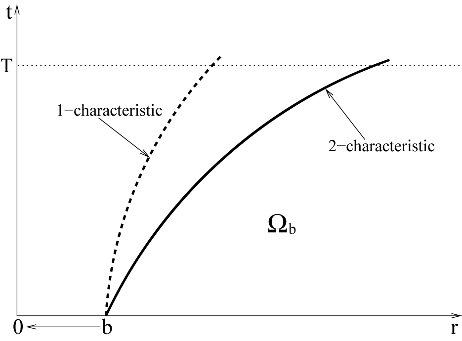
 $\Omega _b=\{(r,t):\ 0\leq t\leq T, r\geq r_2(t; b,0)\}$
and
 $r=r_2(t; b,0)$
is the
 $2$
-characteristic curve starting from point
 $(b,0)$
(see Figure 1 for illustration). Based on the conclusion that the characteristic starting from
 $(r,t)=(0,0)$
must be
 $r=0$
, we let
 $b\rightarrow 0$
to establish the global existence result on the entire half line
 $[0,\infty )$
. On the other hand, for the compressive initial data
 $\alpha (r,0)<0, \beta (r,0)<0$
, we employ their Riccati type equations to prove that
 $\alpha (r,t)<0, \beta (r,t)<0$
in the region of existence of smooth solutions. If
 $-\alpha (r,0)$
or
 $-\beta (r,0)$
is further assumed to be sufficiently large somewhere at a certain point, then the smooth solution may form singularities in finite time.
The region
 $\Omega _b$
.

The rest of the article is organized as follows. In Section 2, we introduce the Riemann variables for system (1.4) and provide the main result of the article. Section 3 is devoted to deriving the Riccati type equations of
 $(\alpha , \beta )$
. In Section 4, we establish invariant domains for the Riemann variables and the rarefaction characters
 $(\alpha , \beta )$
, from which we obtain the a priori
 $C^1$
estimates of the solutions. A positive lower bound estimate for density that is only time-dependent while spatially independent is also deduced in this section. In Section 5, we demonstrate the global existence of
 $C^1$
solution on the entire domain
 $t\geq 0$
,
 $r\geq 0$
for rarefactive initial data. Finally, the singularity formation of smooth solutions is discussed in Section 6.
2 The main results
In this section, we introduce a pair of Riemann variables to transform system (1.4) into a diagonal form and then present the main results of the article.
We consider smooth solutions of system (1.4) with (1.2), in which case the system can be rewritten as
 $$ \begin{align} \textbf{A}\textbf{U}_{t}+\textbf{B}\textbf{U}_{r}=\textbf{F}, \end{align} $$
where the variables and the coefficient matrices are
 $$ \begin{align*} \textbf{U}=&\left( \begin{array}{c} \rho \\ u \end{array} \right),\quad \quad \textbf{F}=-\frac{(d-1)(\rho+\varepsilon A\rho^{\gamma})u}{(1-\varepsilon u^{2})r}\left( \begin{array}{c} \displaystyle 1 \\ \displaystyle u \end{array} \right), \end{align*} $$
and
 $$ \begin{align*} \textbf{A}&=\left( \begin{array}{cc} \displaystyle \frac{1+\varepsilon^2 A\gamma\rho^{\gamma-1}u^{2}}{1-\varepsilon u^{2}} & \displaystyle \frac{2\varepsilon (\rho+\varepsilon A\rho^{\gamma})u}{(1-\varepsilon u^{2})^{2}}\\[8pt] \displaystyle \frac{(1+\varepsilon A\gamma\rho^{\gamma-1})u}{1-\varepsilon u^{2}} & \displaystyle \frac{(\rho+\varepsilon A\rho^{\gamma})(1+\varepsilon u^{2})}{(1-\varepsilon u^{2})^{2}} \end{array} \right),\\\textbf{B}&=\left( \begin{array}{cc} \displaystyle \frac{(1+\varepsilon A\gamma\rho^{\gamma-1})u}{1-\varepsilon u^{2}} & \displaystyle \frac{(\rho+\varepsilon A\rho^{\gamma})(1+\varepsilon u^{2})}{(1-\varepsilon u^{2})^{2}}\\[8pt] \displaystyle \frac{A\gamma\rho^{\gamma-1}+u^{2}}{1-\varepsilon u^{2}} & \displaystyle \frac{2(\rho+\varepsilon A\rho^{\gamma})u}{(1-\varepsilon u^{2})^{2}} \end{array} \right). \end{align*} $$
The eigenvalues of (2.1) are defined by finding the roots of
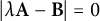 $|\lambda \textbf {A}-\textbf {B}|=0$
, which are given in (1.9). The corresponding right eigenvectors of
 $\lambda _1$
and
 $\lambda _2$
are, respectively,
 $$ \begin{align*} \textbf{R}_{1}=\bigg(-\frac{\sqrt{A\gamma\rho^{\gamma-1}}}{\rho+\varepsilon A\rho^{\gamma}}, \frac{1}{1-\varepsilon u^{2}}\bigg)^{\mathsf{T}}, \quad \textbf{R}_{2}=\bigg(\frac{\sqrt{A\gamma\rho^{\gamma-1}}}{\rho+\varepsilon A\rho^{\gamma}}, \frac{1}{1-\varepsilon u^{2}}\bigg)^{\mathsf{T}}. \end{align*} $$
One can check that there hold
 $\nabla \lambda _i\cdot \textbf {R}_i\neq 0$
for
 $0<\rho <\rho ^*$
, which means that system (2.1) is strictly hyperbolic and genuinely nonlinear.
Let the symbol a represent the sound speed, that is,
 $a=\sqrt {p_{\rho }}=\sqrt {A\gamma }\rho ^{\frac {\gamma -1}{2}}$
with
 $\gamma>1$
satisfying the relativistic constraint
 $a<1/\sqrt {\varepsilon }$
. We rewrite system (2.1) as follows:
 $$ \begin{align} \left\{ \begin{array}{l} \displaystyle \frac{2\gamma}{\gamma-1}\frac{\varepsilon au(1-\varepsilon u^2)}{\gamma+\varepsilon a^2}\partial_ta+\partial_tu +\frac{2\gamma}{\gamma-1}\frac{(1-\varepsilon u^2)a}{\gamma+\varepsilon a^2}\partial_ra +u\partial_ru =0, \\[3mm] \displaystyle \frac{2\gamma}{\gamma-1}\frac{1-\varepsilon u^2}{\gamma+\varepsilon a^2}\partial_ta+\varepsilon au\partial_tu +\frac{2\gamma}{\gamma-1}\frac{1-\varepsilon u^2}{\gamma+\varepsilon a^2}u\partial_ra+a\partial_ru \\[3mm] =-\frac{d-1}{r}(1-\varepsilon u^2)ua. \end{array} \right. \end{align} $$
The eigenvalues
 $\lambda _1$
and
 $\lambda _2$
in (1.9) become
 $$ \begin{align} \lambda_1=\frac{u-a}{1-\varepsilon au}, \quad \lambda_2=\frac{u+a}{1+\varepsilon au}. \end{align} $$
Introduce the Riemann variables
 $w_\pm =w_\pm (u,a)$
 $$ \begin{align} \begin{aligned} &w_{+}=\frac{1}{2\sqrt{\varepsilon}}\ln{\Big(\frac{1+\sqrt{\varepsilon}u}{1-\sqrt{\varepsilon}u}\Big)} +\frac{2\sqrt{\gamma}}{\sqrt{\varepsilon}(\gamma-1)}\arctan{\Big(\sqrt{\frac{\varepsilon}{\gamma}}a\Big)}. \\[1mm] &w_{-}=\frac{1}{2\sqrt{\varepsilon}}\ln{\Big(\frac{1+\sqrt{\varepsilon}u}{1-\sqrt{\varepsilon}u}\Big)} -\frac{2\sqrt{\gamma}}{\sqrt{\varepsilon}(\gamma-1)}\arctan{\Big(\sqrt{\frac{\varepsilon}{\gamma}}a\Big)}, \end{aligned}\end{align} $$
from which one has
 $$ \begin{align} \begin{aligned}u(w_+,w_-)=&\frac{e^{\sqrt{\varepsilon}(w_++w_-)}-1}{\sqrt{\varepsilon}(e^{\sqrt{\varepsilon}(w_++w_-)}+1)}, \\[3mm] a(w_+,w_-)=&\sqrt{\frac{\gamma}{\varepsilon}}\tan{\Big(\frac{\sqrt{\varepsilon}(\gamma-1)} {4\sqrt{\gamma}}(w_+-w_-)\Big)}. \end{aligned}\end{align} $$
Then, we can obtain the governing equations for
 $(w_+,w_-)$
 $$ \begin{align} &\displaystyle \frac{\partial{w_+}}{\partial t}+\lambda_2 \frac{\partial{w_+}}{\partial r}= -\frac{d-1}{r}\frac{au}{1+\varepsilon au}, \end{align} $$
 $$ \begin{align} &\displaystyle \frac{\partial{w_-}}{\partial t}+\lambda_1 \frac{\partial{w_-}}{\partial r}= \frac{d-1}{r}\frac{au}{1-\varepsilon au}. \end{align} $$
We next supply the assumptions of the article.
Assumption 1 Let the adiabatic constant
 $\gamma $
be in the interval
 $1<\gamma <3$
. For any given
 $b>0$
, the initial data
 $(\rho _0(r),u_0(r))=(\rho (r,0),u(r,0))$
of (2.1) make the following inequalities hold:
 $$ \begin{align} 0\leq w_{-}(r,0)<w_{+}(r,0)\leq C:=\frac{1}{2\sqrt{\varepsilon}}\ln{\Big(\frac{7-\gamma}{1+\gamma}\Big)}, \end{align} $$
for any
 $r\in (b,\infty )$
, where
 $$ \begin{align} w_{\pm}(r,0)=\frac{1}{2\sqrt{\varepsilon}} \ln{\Big(\frac{1+\sqrt{\varepsilon}u_0(r)}{1-\sqrt{\varepsilon}u_0(r)}\Big)} \pm\frac{2\sqrt{\gamma}}{\sqrt{\varepsilon}(\gamma-1)} \arctan{\Big(\sqrt{\frac{\varepsilon}{\gamma}}a_0(r)\Big)}, \end{align} $$
and
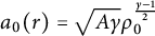 $a_0(r)=\sqrt {A\gamma }\rho _0^{\frac {\gamma -1}{2}}$
.
Remark 1 The inequalities in (2.8) form an invariant domain of
 $(w_-, w_+)$
holding for any time before singularity formation.
We now set
 $$ \begin{align} \begin{aligned}\alpha_0(r)=&\frac{u^{\prime}_0(r)}{1-\varepsilon u^2_0(r)}+\frac{2\gamma}{\gamma-1}\frac{a^{\prime}_0(r)}{\gamma+\varepsilon a^2_0(r)} +\frac{d-1}{r}\frac{u_0(r)a_0(r)}{u_0(r)+a_0(r)}, \\ \beta_0(r)=&\frac{u^{\prime}_0(r)}{1-\varepsilon u^2_0(r)}-\frac{2\gamma}{\gamma-1}\frac{a^{\prime}_0(r)}{\gamma+\varepsilon a^2_0(r)} -\frac{d-1}{r}\frac{u_0(r)a_0(r)}{u_0(r)-a_0(r)}. \end{aligned}\end{align} $$
Assumption 2 Let the adiabatic constant
 $\gamma $
be in the interval
 $1<\gamma <3$
. For the initial data
 $(\rho _0(r),u_0(r))=(\rho (r,0),u(r,0))$
of (2.1), there exists a uniform constant
 $M>0$
such that
 $$ \begin{align} \min_{r\in[0,\infty)}\{\alpha_0(r),\beta_0(r)\}\geq0, \quad \max_{r\in[0,\infty)}\{\alpha_0(r),\beta_0(r)\}<M, \end{align} $$
where
 $\alpha _0(0)=\lim _{r\to 0^+}\alpha _0(r)$
and
 $\beta _0(0)=\lim _{r\to 0^+}\beta _0(r)$
are assumed to exist and nonnegative.
Remark 2 The inequalities in (2.10) form an invariant domain of
 $(\alpha , \beta )$
holding for any time before singularity formation.
Then, the main results of the article can be stated as follows.
Theorem 2.1 Let the initial data
 $(\rho _0(r),u_0(r))\in C^1([0,\infty ))$
satisfy Assumptions 1 and 2. We further assume
 $\rho _0(0)=u_0(0)=0$
,
 $\rho _0(r)>0$
for
 $r>0$
. Then, the radially symmetric relativistic Euler equations (1.4) with (1.2) admit a global
 $C^1$
solution
 $(\rho ,u)(r,t)$
on the entire domain
 $r\geq 0$
,
 $t\geq 0$
. Moreover, the solution satisfies
 $\rho (0,t)=0$
and
 $u(0,t)=0$
and
 $$ \begin{align} \sqrt{\frac{2A\gamma}{\gamma-1}}\rho^{\frac{\gamma-1}{2}}(r,t)\leq u(r,t)\leq \frac{3-\gamma}{4\sqrt{\varepsilon}}, \quad \rho(r,t)>0, \quad \forall\ r\geq0, t\geq0, \end{align} $$
and
 $$ \begin{align} \min_{r\geq0,t\geq0}(\alpha,\beta)(r,t)\geq0, \quad \max_{r\geq0,t\geq0}(\alpha,\beta)(r,t)<M. \end{align} $$
Theorem 2.2 Let the initial data
 $(\rho _0(r),u_0(r))\in C^1((b,\infty ))$
with
 $b>0$
satisfy Assumption 1 and the following compression conditions:
 $$ \begin{align} \alpha_0(r)<0,\quad \beta_0(r)<0,\quad \forall\ r\in[b,\infty). \end{align} $$
Then, there exists a constant
 $N(b, T)$
, depending on b and T, such that, if
 $$ \begin{align} \alpha_0(r^*)\leq -N(b, T),\ \mathrm{or}\ \beta_0(r^*)\leq -N(b, T), \end{align} $$
for some number
 $r^*>b$
, then singularity forms before time T.
Remark 3 The precise form of the constant
 $N(b, T)$
will be given along with the analysis of the problem in Section 6.
3 The Riccati type equations
In this section, we derive the Riccati type equations of
 $(\alpha , \beta )$
, which play a very important role in our analysis below.
We first calculate the rarefaction characters
 $\alpha $
and
 $\beta $
introduced in (1.7). According to the definition of
 $\partial _1$
in (1.8), we directly compute by (2.2)
 $$ \begin{equation} \begin{aligned} &\quad \partial_1\Big(r^{d-1}\frac{\rho+\varepsilon p}{1-\varepsilon u^2}u\Big) \\ &= \partial_t\Big(r^{d-1}\frac{\rho+\varepsilon p}{1-\varepsilon u^2}u\Big) +\frac{u-a}{1-\varepsilon au}\partial_r\Big(r^{d-1}\frac{\rho+\varepsilon p}{1-\varepsilon u^2}u\Big) \\ &=-\partial_r\Big(r^{d-1}\frac{\rho+\varepsilon p}{1-\varepsilon u^2}u^2\Big)-r^{d-1}\partial_rp +\frac{u-a}{1-\varepsilon au}\partial_r\Big(r^{d-1}\frac{\rho+\varepsilon p}{1-\varepsilon u^2}u\Big) \\ &=-r^{d-1}\frac{\rho+\varepsilon p}{1-\varepsilon u^2}\Big\{u\partial_ru+\frac{a(1+\varepsilon u^2)}{1-\varepsilon au}\partial_ru +\frac{d-1}{r}\frac{au(1-\varepsilon u^2)}{1-\varepsilon au}\Big\} \\ &\quad -r^{d-1}\frac{a(a+u)}{1-\varepsilon au}\partial_r\rho \\ &=-r^{d-1}(\rho+\varepsilon p)\frac{a+u}{1-\varepsilon au}\Big(\frac{\partial_ru}{1-\varepsilon u^2}+\frac{d-1}{r}\frac{ua}{u+a}\Big) \\ &\quad -r^{d-1}\frac{2}{\gamma-1}\frac{\rho(a+u)}{1-\varepsilon au}\partial_ra. \end{aligned}\end{equation} $$
The last step in (3.1) is used the relation
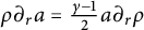 $\rho \partial _ra=\frac {\gamma -1}{2}a\partial _r\rho $
. It follows by (3.1) that
 $$ \begin{align} \begin{aligned} \alpha&=-\frac{\partial_1(r^{d-1}\frac{\rho+\varepsilon p}{1-\varepsilon u^2}u)}{r^{d-1}(\rho+\varepsilon p)\frac{u+a}{1-\varepsilon ua}} \\ &=\frac{\partial_ru}{1-\varepsilon u^2}+\frac{2}{\gamma-1}\frac{\rho \partial_ra}{\rho+\varepsilon p}+\frac{d-1}{r}\frac{ua}{u+a} \\ &=\frac{\partial_ru}{1-\varepsilon u^2}+\frac{2\gamma}{\gamma-1}\frac{\partial_ra}{\gamma+\varepsilon a^2}+\frac{d-1}{r}\frac{ua}{u+a} \\ &=\partial_rw_+ +\frac{d-1}{r}\frac{ua}{u+a}. \end{aligned}\end{align} $$
Analogously, one has
 $$ \begin{equation} \begin{aligned}&\quad \partial_2\Big(r^{d-1}\frac{\rho+\varepsilon p}{1-\varepsilon u^2}u\Big) \\ &= \partial_t\Big(r^{d-1}\frac{\rho+\varepsilon p}{1-\varepsilon u^2}u\Big) +\frac{u+a}{1+\varepsilon au}\partial_r\Big(r^{d-1}\frac{\rho+\varepsilon p}{1-\varepsilon u^2}u\Big) \\ &=-r^{d-1}(\rho+\varepsilon p)\frac{u-a}{1+\varepsilon au}\Big(\frac{\partial_ru}{1-\varepsilon u^2}-\frac{d-1}{r}\frac{ua}{u-a}\Big) \\ &\quad +r^{d-1}\frac{2}{\gamma-1}\frac{\rho(u-a)}{1+\varepsilon au}\partial_ra, \end{aligned}\end{equation} $$
which gives
 $$ \begin{equation} \begin{aligned}\beta&=-\frac{\partial_2(r^{d-1}\frac{\rho+\varepsilon p}{1-\varepsilon u^2}u)}{r^{d-1}(\rho+\varepsilon p)\frac{u-a}{1+\varepsilon ua}} \\ &=\frac{\partial_ru}{1-\varepsilon u^2}-\frac{2\gamma}{\gamma-1}\frac{\partial_ra}{\gamma+\varepsilon a^2}-\frac{d-1}{r}\frac{ua}{u-a} \\ &=\partial_rw_- -\frac{d-1}{r}\frac{ua}{u-a}. \end{aligned}\end{equation} $$
We next derive the Riccati equations for the radially symmetric isentropic relativistic Euler equations.
Lemma 3.1 For smooth solutions of (2.1) with
 $\lambda _1\lambda _2\neq 0$
, we have the following Riccati type equations on
 $\alpha $
and
 $\beta $
 $$ \begin{equation} \begin{aligned}\partial_1\beta&=-\frac{1-\varepsilon u^2}{(1-\varepsilon au)^2}\frac{(\gamma+1)(\gamma-\varepsilon a^2)}{4\gamma}\beta^2 \\ &\quad -\frac{1-\varepsilon u^2}{(1-\varepsilon au)^2}\frac{\gamma(3-\gamma)+\varepsilon a^2(1-3\gamma)}{4\gamma}\alpha\beta +A_1\alpha-B_1\beta, \end{aligned}\end{equation} $$
where
 $$ \begin{equation} \begin{aligned}A_1&=\frac{(d-1)(u+a)}{2r(1+\varepsilon au)(u-a)^2}\Big(\frac{\gamma-1}{2}u^2-a^2+\frac{3\gamma-1}{2\gamma}\varepsilon u^2a^2\Big) \\ B_1&=\frac{(d-1)(1-\varepsilon u^2)}{r(u-a)(1-\varepsilon au)^2}\bigg\{\frac{ua}{u+a}\Big(a(1-\varepsilon a^2)+\frac{\gamma-1}{2\gamma}(\gamma+\varepsilon a^2)u\Big) \\ &\quad +\frac{1-\varepsilon au}{2(1-\varepsilon u^2)}\Big(a^2(1-\varepsilon u^2)+\frac{\gamma-1}{2\gamma}u^2(\gamma+\varepsilon a^2)\Big)\bigg\}, \end{aligned}\end{equation} $$
and
 $$ \begin{equation} \begin{aligned}\partial_2\alpha&=-\frac{1-\varepsilon u^2}{(1+\varepsilon au)^2}\frac{(\gamma+1)(\gamma-\varepsilon a^2)}{4\gamma}\alpha^2 \\ &\quad -\frac{1-\varepsilon u^2}{(1+\varepsilon au)^2}\frac{\gamma(3-\gamma)+\varepsilon a^2(1-3\gamma)}{4\gamma}\alpha\beta +A_2\beta-B_2\alpha, \end{aligned}\end{equation} $$
where
 $$ \begin{equation} \begin{aligned}A_2&=\frac{(d-1)(u-a)}{2r(1-\varepsilon au)(u+a)^2}\Big(\frac{\gamma-1}{2}u^2-a^2+\frac{3\gamma-1}{2\gamma}\varepsilon u^2a^2\Big) \\ B_2&=\frac{(d-1)(1-\varepsilon u^2)}{r(u+a)(1+\varepsilon au)^2}\bigg\{\frac{ua}{u-a}\Big(a(1-\varepsilon a^2)-\frac{\gamma-1}{2\gamma}(\gamma+\varepsilon a^2)u\Big) \\ &\quad +\frac{1+\varepsilon au}{2(1-\varepsilon u^2)}\Big(a^2(1-\varepsilon u^2)+\frac{\gamma-1}{2\gamma}u^2(\gamma+\varepsilon a^2)\Big)\bigg\}. \end{aligned}\end{equation} $$
Remark 4 It is obvious that equations (3.5) and (3.7) are homogeneous, i.e., their right-hand sides vanish when
 $\alpha =\beta =0$
. This important property originated from the special selection of
 $\alpha $
and
 $\beta $
is crucial for us to establish the a priori
 $C^1$
estimates of solutions by constructing the invariant domains.
Proof We only derive (3.5) since the derivation of (3.7) is parallel. In view of (3.4), we first have
 $$ \begin{equation} \begin{aligned}\partial_1\beta&=\partial_1\Big(\partial_rw_--\frac{d-1}{r}\frac{ua}{u-a}\Big) \\ &=\partial_1\partial_rw_--\partial_t\Big(\frac{d-1}{r}\frac{ua}{u-a}\Big)-\frac{u-a}{1-\varepsilon au}\partial_r\Big(\frac{d-1}{r}\frac{ua}{u-a}\Big).\end{aligned} \end{equation} $$
Moreover, thanks to (2.7) and (3.4), one obtains
 $$ \begin{equation} \begin{aligned}\partial_1\partial_rw_-&=\frac{u-a}{1-\varepsilon au}\partial_r\Big(\frac{d-1}{r}\frac{ua}{u-a}\Big) \\ &\quad +\frac{d-1}{r}\frac{ua}{u-a}\partial_r\Big(\frac{u-a}{1-\varepsilon au}\Big)-\partial_r\Big(\frac{u-a}{1-\varepsilon au}\Big)\partial_rw_- \\ &=\frac{u-a}{1-\varepsilon au}\partial_r\Big(\frac{d-1}{r}\frac{ua}{u-a}\Big)-\beta\partial_r\Big(\frac{u-a}{1-\varepsilon au}\Big), \end{aligned}\end{equation} $$
which together with (3.9) yields
 $$ \begin{align} \partial_1\beta&=-\beta\partial_r\Big(\frac{u-a}{1-\varepsilon au}\Big)-\partial_t\Big(\frac{d-1}{r}\frac{ua}{u-a}\Big)=\mathcal{I}_1+\mathcal{I}_2, \end{align} $$
where
 $$ \begin{equation} \begin{aligned}\mathcal{I}_1&=-\frac{\beta}{(1-\varepsilon au)^2}\Big\{(1-\varepsilon a^2)\partial_ru-(1-\varepsilon u^2)\partial_ra\Big\}, \\ \mathcal{I}_2&=\frac{d-1}{r(u-a)^2}(a^2\partial_tu-u^2\partial_ta). \end{aligned}\end{equation} $$
To proceed, we next give some relationships among
 $\alpha $
,
 $\beta $
,
 $\partial _tu$
,
 $\partial _ta$
,
 $\partial _ru$
, and
 $\partial _ra$
. Owing to (2.4), one has by directly calculates
 $$ \begin{align*} \partial_rw_++\partial_rw_-=\frac{2\partial_ru}{1-\varepsilon u^2}, \qquad \partial_rw_+-\partial_rw_-=\frac{4\gamma}{\gamma-1}\frac{\partial_ra}{\gamma+\varepsilon a^2}, \end{align*} $$
which together with (3.2), (3.4), and (2.2), we achieve the following formulas:
 $$ \begin{equation} \begin{aligned} \frac{2\partial_ru}{1-\varepsilon u^2}&=\alpha+\beta+\frac{d-1}{r}\frac{2ua^2}{(u-a)(u+a)}, \\ \frac{4\gamma}{\gamma-1}\frac{\partial_ra}{\gamma+\varepsilon a^2}&=\alpha-\beta-\frac{d-1}{r}\frac{2u^2a}{(u-a)(u+a)}, \end{aligned}\end{equation} $$
and
 $$ \begin{equation} \begin{aligned}&\quad \frac{2\gamma}{\gamma-1}\frac{(1-\varepsilon au)(1+\varepsilon au)}{\gamma+\varepsilon a^2}\partial_ta \\ &=-a\partial_ru -\frac{2\gamma}{\gamma-1}\frac{u(1-\varepsilon a^2)}{\gamma+\varepsilon a^2}\partial_ra-\frac{d-1}{r}ua, \\ &\quad \frac{(1-\varepsilon au)(1+\varepsilon au)}{1-\varepsilon u^2}\partial_tu \\ &=-\frac{u(1-\varepsilon a^2)}{1-\varepsilon u^2}\partial_ru -\frac{2\gamma}{\gamma-1}\frac{a(1-\varepsilon u^2)}{\gamma+\varepsilon a^2}\partial_ra+\frac{d-1}{r}\varepsilon a^2u^2. \end{aligned}\end{equation} $$
Then, putting (3.13) and (3.14) into (3.11) and doing simple rearrangements, we acquire
 $$ \begin{align} \mathcal{I}_1=&-\frac{\beta}{(1-\varepsilon au)^2}\Big\{(1-\varepsilon a^2)\partial_ru-(1-\varepsilon u^2)\partial_ra\Big\} \nonumber \\ =&-\frac{\beta}{(1-\varepsilon au)^2}\bigg\{\frac{(1-\varepsilon a^2)(1-\varepsilon u^2)}{2}\Big(\alpha+\beta+\frac{d-1}{r}\frac{2ua^2}{(u-a)(u+a)}\Big) \nonumber \\ &-\frac{\gamma-1}{4\gamma}(1-\varepsilon u^2)(\gamma+\varepsilon a^2)\Big(\alpha-\beta-\frac{d-1}{r}\frac{2u^2a}{(u-a)(u+a)}\Big)\bigg\} \nonumber \\ =&-\frac{d-1}{r}\frac{ua(1-\varepsilon u^2)}{(u-a)(u+a)(1-\varepsilon au)^2}\Big\{a(1-\varepsilon a^2)+\frac{\gamma-1}{2\gamma}(\gamma+\varepsilon a^2)u\Big\}\beta \nonumber \\ &-\frac{1-\varepsilon u^2}{(1-\varepsilon au)^2}\frac{(\gamma+1)(\gamma-\varepsilon a^2)}{4\gamma}\beta^2 \nonumber \\ &-\frac{1-\varepsilon u^2}{(1-\varepsilon au)^2}\frac{\gamma(3-\gamma)+\varepsilon a^2(1-3\gamma)}{4\gamma}\alpha\beta. \end{align} $$
Furthermore, one applies (2.2), (3.13), and (3.14) again to achieve
 $$ \begin{align} &a^2\partial_tu-u^2\partial_ta \nonumber \\ =& -\frac{1}{2(1-\varepsilon^2a^2u^2)} \Big(a^3(1-\varepsilon u^2)^2-\frac{\gamma-1}{2\gamma}(\gamma+\varepsilon a^2)(1-\varepsilon a^2)u^3\Big)(\alpha-\beta) \nonumber \\ &-\frac{ua(1-\varepsilon u^2)}{2(1-\varepsilon^2a^2u^2)}\Big(a(1-\varepsilon a^2) -\frac{\gamma-1}{2\gamma}(\gamma+\varepsilon a^2)u\Big)(\alpha+\beta) \nonumber \\ &+\frac{d-1}{r(1-\varepsilon^2a^2u^2)} \bigg\{\frac{u^4a-u^2a^3}{u^2-a^2}\Big(\varepsilon a^3(1-\varepsilon u^2)+\frac{\gamma-1}{2\gamma}(\gamma+\varepsilon a^2)u\Big) \nonumber \\ & +\frac{u^2a}{u^2-a^2}\Big(a^3(1-\varepsilon u^2)^2 -\frac{\gamma-1}{2\gamma}(\gamma+\varepsilon a^2)(1-\varepsilon a^2)u^3\Big) \nonumber \\ & -\frac{u^2a^3(1-\varepsilon u^2)}{u^2-a^2}\Big(a(1-\varepsilon a^2)-\frac{\gamma-1}{2\gamma}(\gamma+\varepsilon a^2)u\Big)\bigg\}. \end{align} $$
Note that
 $$ \begin{align*} &\frac{u^4a-u^2a^3}{(u-a)(u+a)}\Big(\varepsilon a^3(1-\varepsilon u^2)+\frac{\gamma-1}{2\gamma}(\gamma+\varepsilon a^2)u\Big) \\ &+\frac{u^2a}{(u-a)(u+a)}\Big(a^3(1-\varepsilon u^2)^2 -\frac{\gamma-1}{2\gamma}(\gamma+\varepsilon a^2)(1-\varepsilon a^2)u^3\Big) \\ &-\frac{u^2a^3(1-\varepsilon u^2)}{(u-a)(u+a)}\Big(a(1-\varepsilon a^2)-\frac{\gamma-1}{2\gamma}(\gamma+\varepsilon a^2)u\Big) \\ =&\frac{u^2a(1-\varepsilon u^2)}{(u-a)(u+a)}\Big\{\varepsilon a^3(u^2-a^2)+a^3(1-\varepsilon u^2)-a^3(1-\varepsilon a^2)\Big\} \\ &+\frac{\gamma-1}{2\gamma}\frac{u^2a(\gamma+\varepsilon a^2)}{(u-a)(u+a)}\Big\{u(u^2-a^2)-(1-\varepsilon a^2)u^3+a^2u(1-\varepsilon u^2)\Big\}=0. \end{align*} $$
Utilizing the above fact into (3.16) leads to
 $$ \begin{align} a^2\partial_tu-u^2\partial_ta =&-\frac{u+a}{2(1+\varepsilon ua)}\Big(a^2(1-\varepsilon u^2)- \frac{\gamma-1}{2\gamma}(\gamma+\varepsilon a^2)u^2\Big)\alpha \nonumber \\ &-\frac{u-a}{2(1-\varepsilon au)}\Big(\frac{\gamma-1}{2\gamma}(\gamma+\varepsilon a^2)u^2+a^2(1-\varepsilon u^2)\Big)\beta. \end{align} $$
We insert (3.17) into (3.12) to obtain
 $$ \begin{equation} \begin{aligned}\mathcal{I}_2&=\frac{d-1}{r(u-a)^2}(a^2\partial_tu-u^2\partial_ta) \\ &=-\frac{d-1}{r(u-a)^2}\Big[\frac{u+a}{2(1+\varepsilon ua)}\Big(a^2(1-\varepsilon u^2)- \frac{\gamma-1}{2\gamma}(\gamma+\varepsilon a^2)u^2\Big)\alpha \\ &\quad +\frac{u-a}{2(1-\varepsilon au)}\Big(\frac{\gamma-1}{2\gamma}(\gamma+\varepsilon a^2)u^2+a^2(1-\varepsilon u^2)\Big)\beta\Big]. \end{aligned}\end{equation} $$
One combines (3.11), (3.15), and (3.18) to easily gain (3.5). The proof of the lemma is complete.
4 Invariant domains
In this section, we establish invariant domains for
 $(w_-, w_+)$
and
 $(\alpha , \beta )$
and derive a positive lower bound estimate for the density.
Before studying the solution in the whole domain
 $(r,t)\in \mathbb {R}^{+}\times \mathbb {R}^{+}$
, we first consider the Cauchy problem on the domain
 $\Omega _b$
in the
 $(r,t)$
-plane, where
 $\Omega _b$
is defined as in Figure 1.
Problem 1 For system (2.1) with the initial data
 $(\rho _0(r),u_0(r))=(\rho (r,0),u(r,0))$
, we seek the smooth solution on domain of dependence
 $\Omega _b$
with base
 $t=0$
and
 $r\in (b,\infty )$
for any
 $b>0$
, i.e., domain to the right of the
 $2$
-characteristic starting at
 $(b,0)$
.
Then, we have the following.
Lemma 4.1 Let Assumption 1 hold. Then, any smooth solution of Problem 1 in the domain of dependence
 $\Omega _b$
based on
 $(b,\infty )$
, with
 $b>0$
, satisfies
 $$ \begin{align} 0\leq w_-(r,t)\leq w_+(r,t)\leq C. \end{align} $$
Remark 5 We shall show the fact that
 $w_-<w_+$
(i.e.,
 $\rho>0$
) in
 $\Omega _b$
is true at the end of this section.
Proof We first prove
 $w_-\geq 0$
in
 $\Omega _b$
. Assume that there exists a point
 $(\bar r,\bar t)\in \Omega $
with
 $\bar t>0$
such that
 $w_-(\bar r,\bar t)<0$
. We use
 $l_1$
to denote the
 $1$
-characteristic
 $r=r_1(t)$
through the point
 $(\bar r, \bar t)$
:
 $$ \begin{align*} \frac{\mathrm{d}r_1}{\mathrm{d}t}=\lambda_1(r_1(t),t), \quad r_1(\bar t)=\bar r. \end{align*} $$
Due to
 $w_-(r_1(0),0)\geq 0$
by (2.8), we know that there exist some times
 $0\leq \tilde {t}<\hat {t}\leq \bar {t}$
such that along
 $l_1$
, there hold
 $w_-(r_1(t),t)\geq 0$
for
 $t\in [0,\tilde {t})$
,
 $w_-(r_1(\tilde {t}),\tilde {t})=0$
, and
 $w_-(r_1(t),t)<0$
for
 $t\in (\tilde {t},\hat {t}]$
. Thus,
 $\partial _1w_-(r_1(\tilde {t}),\tilde {t})<0$
. On the other hand, one recalls (2.7) to see that
 $$ \begin{align*} \partial_1w_-(r_1(\tilde{t}),\tilde{t})=\frac{d-1}{r}\frac{au}{1-\varepsilon au}(r_1(\tilde{t}),\tilde{t})\geq0, \end{align*} $$
which leads to a contradiction. Hence, we have
 $w_-(r,t)\geq w_-(r,0)\geq 0$
in
 $\Omega _b$
.
According to the conclusion
 $w_-(r,t)\geq 0$
in
 $\Omega _b$
, it suggests by the expression of
 $w_-$
in (2.4) that
 $$ \begin{align*}\frac{1}{2\sqrt{\varepsilon}}\ln\Big(\frac{1+\sqrt{\varepsilon}u}{1-\sqrt{\varepsilon}u}\Big) \geq\frac{2\sqrt{\gamma}}{\sqrt{\varepsilon}(\gamma-1)}\arctan\Big(\sqrt{\frac{\varepsilon}{\gamma}}a\Big)\geq0, \end{align*} $$
which implies that
 $u(r,t)\geq 0$
in
 $\Omega _b$
. Thus, one has by (2.6)
 $$ \begin{align*} \displaystyle \frac{\partial{w_+}}{\partial t}+\lambda_2 \frac{\partial{w_+}}{\partial r}= -\frac{d-1}{r}\frac{au}{1+\varepsilon au}\leq0, \end{align*} $$
which means that
 $w_+(r_2(t),t)\leq w_+(r_2(0),0)$
along any
 $2$
-characteristic curve
 $r_2(t)$
. Therefore, we attain
 $$ \begin{align} w_+(r,t)\leq w_+(r,0)\leq C. \end{align} $$
The proof of the lemma is finished.
Based on Lemma 4.1, we have the following estimates.
Lemma 4.2 Let Assumption 1 hold. Suppose that the smooth solution of Problem 1 in
 $\Omega _b$
satisfies
 $0<w_-<w_+$
. Then, there hold in the domain
 $\Omega _b$
 $$ \begin{align} \sqrt{\frac{2}{\gamma-1}}a\leq u\leq\frac{3-\gamma}{4\sqrt{\varepsilon}}, \end{align} $$
and
 $$ \begin{align} 0\leq A_i\leq B_i, \end{align} $$
where
 $i=1,2$
,
 $A_i$
and
 $B_i$
are defined in (3.6) and (3.8).
Proof We first combine (2.5), (4.1), and (4.2) to obtain
 $$ \begin{align} \sqrt{\varepsilon}u\leq\frac{e^{2\sqrt{\varepsilon}w_+(t,r)}-1}{e^{2\sqrt{\varepsilon}w_+(t,r)}+1} \leq\frac{e^{2\sqrt{\varepsilon}w_+(0,r)}-1}{e^{2\sqrt{\varepsilon}w_+(0,r)}+1}, \end{align} $$
which together with (2.8) arrives at
 $$ \begin{align} \sqrt{\varepsilon}u\leq \frac{e^{2\sqrt{\varepsilon}w_+(0,r)}-1}{e^{2\sqrt{\varepsilon}w_+(0,r)}+1}\leq\frac{3-\gamma}{4}. \end{align} $$
It is easy to find by the assumption
 $0<w_-<w_+$
that
 $$ \begin{align} \frac{u}{1-\sqrt{\varepsilon}u} \geq&\frac{1}{2\sqrt{\varepsilon}}\ln\Big(\frac{1+\sqrt{\varepsilon}u}{1-\sqrt{\varepsilon}u}\Big) \nonumber \\ \geq&\frac{2\sqrt{\gamma}}{\sqrt{\varepsilon}(\gamma-1)}\arctan\Big(\sqrt{\frac{\varepsilon}{\gamma}}a\Big) \geq\frac{2}{\gamma-1}a\Big(1-\frac{\varepsilon a^2}{3\gamma}\Big). \end{align} $$
In view of (4.7), we calculate
 $$ \begin{align} \frac{\gamma-1}{2}u^2-a^2\geq&\frac{2}{\gamma-1}a^2\Big(1-\frac{\varepsilon a^2}{3\gamma}\Big)(1-\sqrt{\varepsilon}u)^2-a^2 \nonumber \\ \geq&\frac{2}{\gamma-1}a^2\Big[\Big(1-\frac{\varepsilon u^2}{3\gamma}\Big)(1-\sqrt{\varepsilon}u)^2-\frac{\gamma-1}{2}\Big] \nonumber \\ =&\frac{2}{\gamma-1}a^2\mathcal{I}_3, \end{align} $$
where
 $$ \begin{align} \mathcal{I}_3=\ &1-2\sqrt{\varepsilon}u-\frac{\gamma-1}{2}+\frac{3\gamma-2}{3\gamma}\varepsilon u^2 \nonumber \\ &+\frac{2(\sqrt{\varepsilon}u)^3}{3\gamma}(2-\sqrt{\varepsilon}u)+\Big(\frac{\varepsilon u^2}{3\gamma}(1-\sqrt{\varepsilon}u)\Big)^2 \nonumber \\ =\ &2\Big(\frac{3-\gamma}{4}-\sqrt{\varepsilon}u\Big)+\frac{3\gamma-2}{3\gamma}\varepsilon u^2 \nonumber \\ &+\frac{2(\sqrt{\varepsilon}u)^3}{3\gamma}(2-\sqrt{\varepsilon}u)+\Big(\frac{\varepsilon u^2}{3\gamma}(1-\sqrt{\varepsilon}u)\Big)^2 \geq0, \end{align} $$
by (4.6). Combining (4.8) and (4.9) yields for
 $1<\gamma <3$
 $$ \begin{align} a\leq\sqrt{\frac{2}{\gamma-1}}a\leq u,\quad\ \mathrm{and\ then}\ A_i\geq0. \end{align} $$
Then, (4.3) follows from (4.6) and (4.10).
To show
 $B_i\geq A_i$
, we recall the expressions of
 $A_i$
,
 $B_i$
in (3.6) and (3.8) to obtain
 $$ \begin{equation}\begin{aligned} &\quad B_1-A_1 \\ & = \frac{(d-1)(1-\varepsilon u^2)ua}{r(u-a)(u+a)(1-\varepsilon au)^2}\Big(a(1-\varepsilon a^2)+\frac{\gamma-1}{2\gamma}(\gamma+\varepsilon a^2)u\Big) \\ &\quad +\frac{d-1}{2r(u-a)(1-\varepsilon au)}\Big(a^2(1-\varepsilon u^2)+\frac{\gamma-1}{2\gamma}u^2(\gamma+\varepsilon a^2)\Big) \\ &\quad -\frac{(d-1)(u+a)}{2r(1+\varepsilon au)(u-a)^2}\Big(\frac{\gamma-1}{2}u^2-a^2+\frac{3\gamma-1}{2\gamma}\varepsilon u^2a^2\Big), \end{aligned}\end{equation} $$
which gives through basic simplification
 $$ \begin{equation} \begin{aligned}B_1-A_1 &=\frac{(d-1)(1-\varepsilon u^2)(1-\varepsilon a^2)ua^2}{r(u-a)(1-\varepsilon au)} \\ &\quad \times \Big(\frac{1}{(u-a)(1+\varepsilon au)}+\frac{1}{(u+a)(1-\varepsilon au)}\Big) \\ &\quad +\frac{\gamma-1}{2}\frac{(d-1)(1-\varepsilon u^2)(\gamma+\varepsilon a^2)u^2a}{r(u-a)(1-\varepsilon au)} \\ &\quad \times\Big(\frac{1}{(u+a)(1-\varepsilon au)}-\frac{1}{(u-a)(1+\varepsilon au)}\Big) \\ &=\frac{2(d-1)(1-\varepsilon u^2)u^2a^2}{r(u-a)^2(u+a)(1+\varepsilon au)(1-\varepsilon au)^2} \\ &\quad \times \Big((1-\varepsilon a^2)^2-\frac{\gamma-1}{2\gamma}(1-\varepsilon u^2)(\gamma+\varepsilon a^2)\Big). \end{aligned}\end{equation} $$
Similarly, one has
 $$ \begin{align} B_2-A_2 &=\frac{2(d-1)(1-\varepsilon u^2)u^2a^2}{r(u+a)^2(u-a)(1-\varepsilon au)(1+\varepsilon au)^2} \nonumber\\ &\quad \times \Big((1-\varepsilon a^2)^2-\frac{\gamma-1}{2\gamma}(1-\varepsilon u^2)(\gamma+\varepsilon a^2)\Big). \end{align} $$
Furthermore, we find by (4.3) that
 $$ \begin{align*}\varepsilon a^2\leq\frac{(\gamma-1)(3-\gamma)^2}{32}, \end{align*} $$
from which one gains
 $$ \begin{equation} \begin{aligned}&\quad (1-\varepsilon a^2)^2-\frac{\gamma-1}{2\gamma}(1-\varepsilon u^2)(\gamma+\varepsilon a^2) \\ &\geq(1-\varepsilon a^2)\Big((1-\varepsilon a^2)-\frac{\gamma-1}{2}(\gamma+\varepsilon a^2)\Big) \\ &=\frac{(1-\varepsilon a^2)[\gamma(3-\gamma)-\varepsilon a^2(3\gamma-1)]}{2\gamma} \\ &\geq(1-\varepsilon a^2)\frac{3-\gamma}{2}\Big(1-\frac{(\gamma-1)(3-\gamma)(3\gamma-1)}{32\gamma}\Big)>0. \end{aligned}\end{equation} $$
Substituting (4.14) into (4.12) and (4.13) yields
 $B_i\geq A_i$
. The proof of the lemma is ended.
Remark 6 The second to last inequality in (4.14) implies that the coefficients of term
 $\alpha \beta $
in (3.5) and (3.7) are negative.
We now employ (4.4) to verify that the set
 $\{\min \{\alpha ,\beta \}\geq 0\}$
is an invariant region for Problem
 $1$
.
Lemma 4.3 Consider a smooth solution on
 $t\in [0, T_0]$
for Problem
 $1$
on
 $\Omega _b$
, satisfying Assumption 1 on
 $(b,\infty )$
with
 $b>0$
. We further assume that the functions
 $\alpha _0(r)$
and
 $\beta _0(r)$
defined in (2.10) fulfill
 $$ \begin{align} \min_{r\in[b,\infty)}\{\alpha_0(r), \beta_0(r)\}\geq0. \end{align} $$
Then, the smooth solution satisfies
 $$ \begin{align} \min_{\Omega_b\cap\{t\leq T_0\}}\{\alpha(r,t), \beta(r,t)\}\geq0, \end{align} $$
i.e.,
 $\{(\alpha ,\beta )\vert \min (\alpha ,\beta )\geq 0\}$
is an invariant domain on time.
Remark 7 The proof of the invariant domain
 $\{(\alpha ,\beta )\vert \min (\alpha ,\beta )\geq 0\}$
does not require upper bounds on
 $\alpha _0(r)$
and
 $\beta _0(r)$
.
Proof We first utilize Lemmas 4.1 and 4.2 to estimate the upper bounds of
 $B_i$
. Indeed, the following facts hold:
 $$ \begin{align} \frac{a}{u-a}=&\frac{a}{u-\sqrt{{\frac{2}{\gamma-1}}}a+\sqrt{{\frac{2}{\gamma-1}}}a-a} \nonumber \\ \leq&\frac{a}{\Big(\sqrt{\frac{2}{\gamma-1}}-1\Big)a} =\frac{\sqrt{\gamma-1}(\sqrt{2}+\sqrt{\gamma+1})}{3-\gamma}, \end{align} $$
and
 $$ \begin{align} \frac{u}{u-a}=\ &1+\frac{a}{u-a} \nonumber \\ \leq & 1+\frac{\sqrt{\gamma-1}(\sqrt{2}+\sqrt{\gamma+1})}{3-\gamma} =\frac{2+\sqrt{2(\gamma-1)}}{3-\gamma}, \end{align} $$
which have positive upper bounds for
 $1<\gamma <3$
. Moreover, due to (4.3), one gains
 $$ \begin{align} 1-\varepsilon a^2\geq1-\varepsilon au\geq1-\varepsilon u^2\geq\frac{16-(3-\gamma)^2}{16}>0, \end{align} $$
for
 $1<\gamma <3$
. Thus, it concludes by the expressions of
 $B_1$
,
 $B_2$
in (3.6) and (3.8) that
 $$ \begin{align} B_1,B_2\leq &\frac{d-1}{b}\cdot\frac{1}{(1-\varepsilon au)^2}\bigg\{\frac{ua}{(u-a)(u+a)}\Big(a+\frac{\gamma^2-1}{2\gamma}u\Big) \nonumber \\ &\quad \qquad \quad + \frac{1}{2(1-\varepsilon u^2)(u-a)}\Big(a^2+\frac{\gamma^2-1}{2\gamma}u^2\Big) \bigg\} \nonumber \\ \leq & \frac{(d-1)}{b(1-\varepsilon au)^2(1-\varepsilon u^2)}\Big(a+\frac{\gamma^2-1}{2\gamma}u\Big) \nonumber \\ &\times\bigg\{\frac{\sqrt{\gamma-1}(\sqrt{2}+\sqrt{\gamma+1})}{3-\gamma} +\frac{2+\sqrt{2(\gamma-1)}}{3-\gamma} \bigg\} \nonumber \\ \leq & \frac{16^3(d-1)}{b[16-(3-\gamma)^2]^3} \frac{2+2\sqrt{2(\gamma-1)}+\sqrt{\gamma^2-1}}{3-\gamma}(1+\frac{\gamma^2-1}{2\gamma}) \frac{3-\gamma}{4\sqrt{\varepsilon}} \nonumber \\ \leq & \frac{d-1}{b\sqrt{\varepsilon}}f(\gamma), \end{align} $$
where
 $$ \begin{align*}f(\gamma)=\frac{16^3[(2+2\sqrt{2(\gamma-1)}+\sqrt{\gamma^2-1})(\gamma^2+2\gamma-1)]} {4\gamma[16-(3-\gamma)^2]^3}. \end{align*} $$
Therefore, we have, for all
 $(r,t)\in \Omega _b$
,
 $$ \begin{align} 0\leq A_i(r,t)\leq B_i(r,t)\leq\frac{(d-1)f(\gamma)}{b\sqrt{\varepsilon}}=: K_b, \ \ i=1,2. \end{align} $$
Set
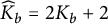 $\widehat {K}_b=2K_b+2$
and
 $\eta>0$
is an arbitrary small number such that
 $$ \begin{align*}\frac{16}{16-(3-\gamma)^2}\cdot \eta e^{\widehat{K}_b t}\leq1. \end{align*} $$
We introduce two new variables for
 $t\leq T_0$
 $$ \begin{align} X=\alpha+\eta e^{\widehat{K}_b t}, \quad Y=\beta+\eta e^{\widehat{K}_b t}. \end{align} $$
According to Lemma 3.1, we can obtain the governing system of
 $(X,Y)$
as follows:
 $$ \begin{equation} \begin{aligned}\partial_2X&=\bigg\{-\frac{1-\varepsilon u^2}{(1+\varepsilon au)^2}\frac{(\gamma+1)(\gamma-\varepsilon a^2)}{4\gamma}(X-2\eta e^{\widehat{K}_b t}) \\ &\quad -\frac{1-\varepsilon u^2}{(1+\varepsilon au)^2}\frac{\gamma(3-\gamma)+\varepsilon a^2(1-3\gamma)}{4\gamma}(Y-\eta e^{\widehat{K}_b t}) -B_2\bigg\}X \\ &\quad +\bigg\{\frac{1-\varepsilon u^2}{(1+\varepsilon au)^2}\frac{\gamma(3-\gamma)+\varepsilon a^2(1-3\gamma)}{4\gamma}\eta e^{\widehat{K}_b t}+A_2\bigg\}Y \\ &\quad +\eta e^{\widehat{K}_b t}\bigg\{\widehat{K}_b-A_2+B_2-\frac{(1-\varepsilon u^2)(1-\varepsilon a^2)}{(1+\varepsilon au)^2}\eta e^{\widehat{K}_b t}\bigg\}, \end{aligned}\end{equation} $$
and
 $$ \begin{equation} \begin{aligned}\partial_1Y&=\bigg\{-\frac{1-\varepsilon u^2}{(1-\varepsilon au)^2}\frac{(\gamma+1)(\gamma-\varepsilon a^2)}{4\gamma}(Y-2\eta e^{\widehat{K}_b t}) \\ &\quad -\frac{1-\varepsilon u^2}{(1-\varepsilon au)^2}\frac{\gamma(3-\gamma)+\varepsilon a^2(1-3\gamma)}{4\gamma}(X-\eta e^{\widehat{K}_b t}) -B_1\bigg\}Y \\ &\quad +\bigg\{\frac{1-\varepsilon u^2}{(1-\varepsilon au)^2}\frac{\gamma(3-\gamma)+\varepsilon a^2(1-3\gamma)}{4\gamma}\eta e^{\widehat{K}_b t}+A_1\bigg\}X \\ &\quad +\eta e^{\widehat{K}_b t}\bigg\{\widehat{K}_b-A_1+B_1-\frac{(1-\varepsilon u^2)(1-\varepsilon a^2)}{(1-\varepsilon au)^2}\eta e^{\widehat{K}_b t}\bigg\}. \end{aligned}\end{equation} $$
From (4.19), one has
 $$ \begin{align*} \frac{(1-\varepsilon u^2)(1-\varepsilon a^2)}{(1+\varepsilon au)^2}\leq &\frac{(1-\varepsilon u^2)(1-\varepsilon a^2)}{(1-\varepsilon au)^2} \\ \leq &\frac{1-\varepsilon a^2}{1-\varepsilon u^2}\leq\frac{16(1-\varepsilon a^2)}{16-(3-\gamma)^2}\leq\frac{16}{16-(3-\gamma)^2}. \end{align*} $$
Thanks to the choice of
 $\widehat {K}_b$
and
 $\eta $
, it suggests that
 $$ \begin{align} &\widehat{K}_b-A_i-B_i-\frac{(1-\varepsilon u^2)(1-\varepsilon a^2)}{(1-\varepsilon au)^2}\eta e^{\widehat{K}_b t} \nonumber \\ \geq & \widehat{K}_b-2 K_b-\frac{16\eta e^{\widehat{K}_b t}}{16-(3-\gamma)^2}\geq1>0, \end{align} $$
which mean that the last terms in (4.23) and (4.24) are strictly positive.
Next, we apply the contradiction argument to confirm
 $\{(X,Y)\vert \min (X,Y)>0\}$
is an invariant domain for
 $t\leq T_0$
. It is easy to see by the initial conditions that
 $X(r,0)>0$
,
 $Y(r,0)>0$
for any
 $r\in [b,\infty )$
. Suppose that there exists some point
 $(r^*,t^*)$
with
 $0<t^*\leq T_0$
in
 $\Omega _b$
such that
 $X(r^*,t^*)=0$
or
 $Y(r^*,t^*)=0$
holds. Owing to the boundedness of the wave speed on
 $[0,t^*]$
, we can draw the 1- and 2-characteristics starting from
 $(r^*,t^*)$
downward up to the line
 $t=0$
and obtain a characteristic triangle
 $\triangle ^*\subset \Omega _b$
. On the basis of the above analysis, we can find the first time
 $T\leq t^*$
such that
 $X(T)=0$
or
 $Y(T)=0$
in
 $\triangle ^*$
. The proof is now divided into two cases.
Case I: At time T,
 $Y=0,$
and
 $X\geq 0$
. In this case, we apply (4.24) and (4.25) to acquire
 $$ \begin{equation} \begin{aligned}\frac{\partial_1Y}{Y}&>-\frac{1-\varepsilon u^2}{(1-\varepsilon au)^2}\frac{(\gamma+1)(\gamma-\varepsilon a^2)}{4\gamma}(Y-2\eta e^{\widehat{K}_b t}) \\ &\quad-\frac{1-\varepsilon u^2}{(1-\varepsilon au)^2}\frac{\gamma(3-\gamma)+\varepsilon a^2(1-3\gamma)}{4\gamma}(X-\eta e^{\widehat{K}_b t}) -B_1, \end{aligned}\end{equation} $$
in the interval
 $[0,T)$
. Integrating (4.26) along the
 $1$
-characteristic
 $r=r_1(t)$
from
 $0$
to
 $s<T$
yields
 $$ \begin{align*} Y(s)=\ &Y(r_1(s),s)>Y(r_1(0),0) \nonumber \\ &\times \exp\bigg\{\int_0^s\Big(-\frac{1-\varepsilon u^2}{(1-\varepsilon au)^2}\frac{(\gamma+1)(\gamma-\varepsilon a^2)}{4\gamma}(Y-2\eta e^{\widehat{K}_b t}) \nonumber \\ &-\frac{1-\varepsilon u^2}{(1-\varepsilon au)^2}\frac{\gamma(3-\gamma)+\varepsilon a^2(1-3\gamma)}{4\gamma}(X-\eta e^{\widehat{K}_b t}) -B_1\Big)(r_1(t),t)\ \mathrm{d}t\bigg\}, \end{align*} $$
which contradicts the fact that s is finite.
Case II: At time T,
 $X=0$
, and
 $Y\geq 0$
. In this case, we employ (4.23) and (4.25) to obtain
 $$ \begin{align} \begin{aligned}\frac{\partial_2X}{X}>-\frac{1-\varepsilon u^2}{(1+\varepsilon au)^2}\frac{(\gamma+1)(\gamma-\varepsilon a^2)}{4\gamma}(X-2\eta e^{\widehat{K}_b t}) \\ -\frac{1-\varepsilon u^2}{(1+\varepsilon au)^2}\frac{\gamma(3-\gamma)+\varepsilon a^2(1-3\gamma)}{4\gamma}(Y-\eta e^{\widehat{K}_b t}) -B_2, \end{aligned}\end{align} $$
subsequently
 $$ \begin{align*} X(s)=\ &X(r_2(s),s)>X(r_2(s_0),s_0) \nonumber \\ &\times \exp\bigg\{\int_{s_0}^s\Big(-\frac{1-\varepsilon u^2}{(1+\varepsilon au)^2}\frac{(\gamma+1)(\gamma-\varepsilon a^2)}{4\gamma}(X-2\eta e^{\widehat{K}_b t}) \nonumber \\ &-\frac{1-\varepsilon u^2}{(1+\varepsilon au)^2}\frac{\gamma(3-\gamma)+\varepsilon a^2(1-3\gamma)}{4\gamma}(Y-\eta e^{\widehat{K}_b t}) -B_2\Big)(r_2(t),t)\ \mathrm{d}t\bigg\}, \end{align*} $$
which also means by the initial conditions that s cannot be finite. This leads a contradiction.
Therefore, we have
 $$ \begin{align*}X=\alpha(r,t)+\eta e^{\widehat{K}_b t}>0, \quad Y=\beta(r,t)+\eta e^{\widehat{K}_b t}>0, \end{align*} $$
for
 $t\leq T_0$
and any
 $\eta $
satisfying
 $\eta e^{\widehat {K}_b T_0}<1$
. It follows by the arbitrariness of
 $\eta>0$
that
 $$ \begin{align*}\alpha(r,t)\geq0, \ \ \beta(r,t)\geq0,\quad \forall\ (r,t)\in\Omega_b\cap\{t\leq T_0\}, \end{align*} $$
which is the desired result (4.16). The proof of the lemma is complete.
We next establish another invariant domain on the upper bounds of
 $\alpha $
and
 $\beta $
.
Lemma 4.4 Consider a smooth solution on
 $t\in [0,T_0]$
for Problem 1 on
 $\Omega _b$
, satisfying Assumption 1 on
 $(b,\infty )$
with
 $b>0$
. We further assume that the functions
 $\alpha _0(r)$
and
 $\beta _0(r)$
defined in (2.10) fulfill
 $$ \begin{align} \min_{requation[b,\infty)}\{\alpha_0(r), \beta_0(r)\}\geq0, \quad \min_{r\in[b,\infty)}(\alpha_0(r),\beta_0(r))<M, \end{align} $$
for some positive constant M. Then, the smooth solution satisfies
 $$ \begin{align} \max_{\Omega_b\cap\{t\leq T_0\}}\{\alpha(r,t), \beta(r,t)\}<M. \end{align} $$

Proof We first rewrite the equations of
 $\alpha $
and
 $\beta $
in Lemma 3.1 as follows:
 $$ \begin{equation} \begin{aligned}\partial_1\beta&=-\frac{1-\varepsilon u^2}{(1-\varepsilon au)^2}\frac{(\gamma+1)(\gamma-\varepsilon a^2)}{4\gamma}\beta^2 \\ &\quad -\frac{1-\varepsilon u^2}{(1-\varepsilon au)^2}\frac{\gamma(3-\gamma)+\varepsilon a^2(1-3\gamma)}{4\gamma}\alpha\beta \\ &\quad +A_1(\alpha-\beta)-(B_1-A_1)\beta, \end{aligned}\end{equation} $$
and
 $$ \begin{equation} \begin{aligned}\partial_2\alpha&=-\frac{1-\varepsilon u^2}{(1+\varepsilon au)^2}\frac{(\gamma+1)(\gamma-\varepsilon a^2)}{4\gamma}\alpha^2 \\ &\quad -\frac{1-\varepsilon u^2}{(1+\varepsilon au)^2}\frac{\gamma(3-\gamma)+\varepsilon a^2(1-3\gamma)}{4\gamma}\alpha\beta \\ &\quad +A_2(\beta-\alpha)-(B_2-A_2)\alpha. \end{aligned}\end{equation} $$
Recalling (4.4) yields
 $B_i-A_i\geq 0 (i=1,2)$
.
We verify the conclusion of the lemma by utilizing the contradiction argument again. As in the proof of Lemma 4.3, we may assume that there exists a characteristic triangle tip at
 $(\bar r, T)$
such that
 $\alpha =M$
or
 $\beta =M$
at
 $(\bar r, T)$
, but
 $0\leq \alpha <M$
and
 $0\leq \beta <M$
in the characteristic triangle. Without loss of generality, we assume
 $0\leq \alpha <M$
and
 $\beta =M$
at
 $(\bar r, T)$
. Then, it is clear by (4.30) that
 $$ \begin{align*} &\partial_1\beta(\bar r, T) \\ & <\bigg\{-\frac{1-\varepsilon u^2}{(1-\varepsilon au)^2}\Big(\frac{(\gamma+1)(\gamma-\varepsilon a^2)}{4\gamma}\beta^2 +\frac{\gamma(3-\gamma)+\varepsilon a^2(1-3\gamma)}{4\gamma}\alpha\beta\Big)\bigg\}\bigg|_{(\bar r, T)} \\ & <0, \end{align*} $$
which contradicts to the assumption that
 $\beta <M$
in the characteristic triangle. A similar contradiction when
 $0\leq \beta <M$
and
 $\alpha =M$
at
 $(\bar r, T)$
can be obtained by (4.31). This finishes the proof of the lemma.
At the end of this section, we derive an only time-dependent density positive lower bound, which directly leads to
 $w_-<w_+$
by (2.4).
Lemma 4.5 Let the assumption in Lemma 4.4 hold. Moreover, suppose that the initial data satisfy
 $$ \begin{align} \underline{\rho}:=\min_{r\in[b,\infty)}\rho(r,0)>0. \end{align} $$
Then, the smooth solution for Problem 1 satisfies
 $$ \begin{align} \rho(r,t)\geq \underline{\rho} \Big(\frac{4b\sqrt{\varepsilon}}{4b\sqrt{\varepsilon}+(3-\gamma)t}\Big)^{d-1} e^{-M_bt}, \end{align} $$
for
 $(r,t)\in \Omega _b\cap \{t\leq T_0\}$
, where
 $M_b$
is a positive constant depending on b.
Proof Set
 $\partial _0=\partial _t+u\partial _r$
. Thanks to the definitions of
 $(\partial _1, \partial _2)$
, we attain
 $$ \begin{align} \partial_0=\frac{(1-\varepsilon au)\partial_1+(1+\varepsilon au)\partial_2}{2}. \end{align} $$
Next, we derive the equation for
 $\partial _0a$
. Applying the definitions of
 $(\partial _1,\partial _2)$
again, we calculate by (3.13) and (3.14),
 $$ \begin{align} \partial_2a&=\partial_ta+\frac{u+a}{1+\varepsilon au}\partial_ra \nonumber \\ =&-\frac{\gamma-1}{2\gamma}\frac{\gamma+\varepsilon a^2}{1-\varepsilon^2a^2u^2} \Big(\frac{d-1}{r}ua+\frac{2\gamma}{\gamma-1}\frac{u(1-\varepsilon a^2)}{\gamma+\varepsilon a^2}\partial_ra+a\partial_ru\Big) +\frac{u+a}{1+\varepsilon au}\partial_ra \nonumber \\ =&\frac{\gamma-1}{4\gamma}\frac{(u+a)(\gamma+\varepsilon a^2)}{1+\varepsilon au}\Big(\alpha-\beta-\frac{d-1}{r}\frac{2u^2a}{(u-a)(u+a)}\Big) \nonumber \\ & -\frac{d-1}{r}\frac{\gamma-1}{2\gamma}\frac{ua(\gamma+\varepsilon a^2)}{1-\varepsilon^2a^2u^2} \nonumber \\ &-\frac{\gamma-1}{4\gamma}\frac{u(1-\varepsilon a^2)(\gamma+\varepsilon a^2)}{1-\varepsilon^2a^2u^2}\Big(\alpha-\beta-\frac{d-1}{r}\frac{2u^2a}{(u-a)(u+a)}\Big) \nonumber \\ &-\frac{\gamma-1}{2\gamma}\frac{a(\gamma+\varepsilon a^2)(1-\varepsilon u^2)}{2(1-\varepsilon^2a^2u^2)}\Big(\alpha+\beta+\frac{d-1}{r}\frac{2ua^2}{(u-a)(u+a)}\Big). \end{align} $$
Doing a simplification for (4.35) obtains
 $$ \begin{align} \partial_2a =-\frac{\gamma-1}{2\gamma}\frac{\gamma+\varepsilon a^2}{1-\varepsilon^2a^2u^2}\Big(\frac{d-1}{r}\frac{u^2a(1-\varepsilon au)}{u-a}+a(1-\varepsilon u^2)\beta\Big). \end{align} $$
A similar computations gives
 $$ \begin{equation} \begin{aligned}\partial_1a&=\partial_ta+\frac{u-a}{1-\varepsilon au}\partial_ra \\ &=-\frac{\gamma-1}{2\gamma}\frac{\gamma+\varepsilon a^2}{1-\varepsilon^2a^2u^2}\Big(\frac{d-1}{r}\frac{u^2a(1+\varepsilon au)}{u+a}+a(1-\varepsilon u^2)\alpha\Big). \end{aligned}\end{equation} $$
Inserting (4.36) and (4.37) into (4.34) leads to
 $$ \begin{equation} \begin{aligned}\partial_0a&= \frac{(1-\varepsilon au)\partial_1a+(1+\varepsilon au)\partial_2a}{2} \\ &=-\frac{\gamma-1}{4\gamma}\bigg\{\frac{\gamma+\varepsilon a^2}{1+\varepsilon au}\Big(\frac{d-1}{r}\frac{u^2a(1+\varepsilon au)}{u+a}+a(1-\varepsilon u^2)\alpha\Big) \\ &\quad +\frac{\gamma+\varepsilon a^2}{1-\varepsilon au}\Big(\frac{d-1}{r}\frac{u^2a(1-\varepsilon au)}{u-a}+a(1-\varepsilon u^2)\beta\Big)\bigg\}\\ &=-\frac{\gamma-1}{4\gamma}(\gamma+\varepsilon a^2)a \\ &\quad \times\Big\{\frac{d-1}{r}\frac{u^2}{u-a}+\frac{d-1}{r}\frac{u^2}{u+a}+\frac{1-\varepsilon u^2}{1-\varepsilon au}\beta +\frac{1-\varepsilon u^2}{1+\varepsilon au}\alpha \Big\}. \end{aligned}\end{equation} $$
Then, we employ the relationship between
 $\rho $
and a to acquire
 $$ \begin{align*} \partial_0\Big(\frac{1}{r^{d-1}\rho}\Big) &=-\frac{1}{r^{d-1}\rho}\frac{d-1}{r}\partial_0r+\frac{1}{r^{d-1}\rho^2}\partial_0\rho \\ &=\frac{1}{r^{d-1}\rho}\Big(-\frac{2}{\gamma-1}\frac{1}{a}\partial_0a-\frac{d-1}{r}\partial_0r\Big) \\ &=\frac{1}{r^{d-1}\rho}\Big\{\frac{\gamma+\varepsilon a^2}{2\gamma}\Big(\frac{d-1}{r}\frac{u^2}{u-a}+\frac{d-1}{r}\frac{u^2}{u+a} +\frac{1-\varepsilon u^2}{1-\varepsilon au}\beta+\frac{1-\varepsilon u^2}{1+\varepsilon au}\alpha \Big) \\ &\quad-\frac{d-1}{r}u\Big\}, \end{align*} $$
from which one derives
 $$ \begin{align} &\partial_0\ln\Big(\frac{1}{r^{d-1}\rho}\Big) \nonumber \\ =&\frac{\gamma+\varepsilon a^2}{2\gamma}\Big(\frac{d-1}{r}\frac{u^2}{u-a}+\frac{d-1}{r}\frac{u^2}{u+a}+\frac{1-\varepsilon u^2}{1-\varepsilon au}\beta +\frac{1-\varepsilon u^2}{1+\varepsilon au}\alpha \Big)-\frac{d-1}{r}u \nonumber \\ =&\frac{(d-1)(\gamma+\varepsilon u^2)}{2r\gamma}\Big(\frac{a^2}{u-a}+\frac{a^2}{u+a}\Big) \nonumber \\ &+\frac{(\gamma+\varepsilon a^2)(1-\varepsilon u^2)}{2\gamma}\Big(\frac{\beta}{1-\varepsilon au}+\frac{\alpha}{1+\varepsilon au}\Big). \end{align} $$
Recalling (4.3) and (4.17) and applying the fact
 $r\geq b$
for any point
 $(r,t)\in \Omega _b$
, there hold
 $$ \begin{align} \begin{array}{r} \frac{1}{1+\varepsilon au}\leq\frac{1}{1-\varepsilon au}\leq\frac{1}{1-\varepsilon u^2}, \\[3mm] \frac{(d-1)(\gamma+\varepsilon u^2)}{2r\gamma}\leq\frac{(d-1)(\gamma+1)}{2b\gamma}, \end{array} \quad \begin{array}{r} \frac{\gamma+\varepsilon a^2}{2\gamma}\leq\frac{\gamma+1}{2\gamma}\leq1, \\[3mm] \frac{a^2}{u+a}\leq\frac{a^2}{u-a}\leq\frac{(\gamma-1)(\sqrt{2}+\sqrt{\gamma+1})}{4\sqrt{2\varepsilon}}. \end{array} \end{align} $$
Putting (4.39) into (4.39) achieves
 $$ \begin{equation} \begin{aligned}\partial_0\ln\Big(\frac{1}{r^{d-1}\rho}\Big)&\leq \frac{(d-1)(\gamma^2-1)(\sqrt{2}+\sqrt{\gamma+1})}{4b\gamma\sqrt{2\varepsilon}}+\beta+\alpha \\ &\leq \frac{(d-1)(\gamma^2-1)(\sqrt{2}+\sqrt{\gamma+1})}{4b\gamma\sqrt{2\varepsilon}}+2M =: M_b. \end{aligned}\end{equation} $$
For any point
 $(\nu , \mu )\in \Omega _b\cap \{t\leq T_0\}$
, we define the curve
 $r=r_0(t)=r_0(t;\nu ,\mu )\ (t\leq \mu )$
by
 $$ \begin{align} \frac{\mathrm{d}r_0(t)}{\mathrm{d}t}=u(r_0(t),t), \quad r_0(\mu)=\nu. \end{align} $$
Denote the intersection point of
 $r=r_0(t)$
and the initial line
 $t=0$
by
 $(r_0,0)$
. Then, one has
 $$ \begin{align} r_0 \leq r_0(t)\leq r_0 +\int_{0}^{t} u(r_0(\tau),\tau) \mathrm{d}\tau \leq r_0+\frac{3-\gamma}{4\sqrt{\varepsilon}}t, \end{align} $$
which leads to
 $$ \begin{align} \frac{r_0}{r_0(t)}\geq \frac{4b\sqrt{\varepsilon}}{4b\sqrt{\varepsilon}+(3-\gamma)t}. \end{align} $$
Now, we integrate (4.41) along
 $r_0(t)$
to conclude that
 $$ \begin{equation} \begin{aligned}\rho(r,t)&\geq \Big(\frac{r_0(t_0)}{r_0(t)}\Big)^{d-1}\rho_0(r_0)e^{-M_bt} \\ &\geq \rho_0(r_0) \Big(\frac{4b\sqrt{\varepsilon}}{4b\sqrt{\varepsilon}+(3-\gamma)t}\Big)^{d-1}e^{-M_bt} \\ &\geq \underline{\rho} \Big(\frac{4b\sqrt{\varepsilon}}{4b\sqrt{\varepsilon}+(3-\gamma)t}\Big)^{d-1} e^{-M_bt}, \end{aligned}\end{equation} $$
which is the desired estimate (4.33). The proof of the lemma is ended.
Remark 9 A density positive lower bound that is only linear about time was previously established by Cai, Chen, and Wang [Reference Cai, Chen and Wang6] for the classical radially symmetric isentropic Euler equations (1.5). However, their lower bound also depends on the spatial variable r, especially when
 $r\rightarrow \infty $
, this lower bound tends to zero. In other words, their lower bound is not uniform with respect to spatial variable.
5 Global existence of smooth solutions
In this section, we complete the proof of Theorem 2.1 by establishing the global existence of smooth solutions in
 $\Omega _b$
for Problem 1 and then letting
 $b\to 0$
. These results are based on the
 $L^\infty $
bound in (4.3), the density lower bound in (4.33), and
 $C^1$
bound for
 $w_+$
and
 $w_-$
.
We first have the following existence theorem in
 $\Omega _b$
.
Theorem 5.1 Let the initial data
 $(\rho _0(r),u_0(r))\in C^1([b,\infty ))$
satisfy Assumptions 1 and 2. We further suppose that
 $\underline {\rho }=\min _{r\in [b,\infty )}\rho _0(r)>0$
. Then, Problem 1 admits a global
 $C^1$
solution on the domain of dependence
 $\Omega _b$
on the
 $(r,t)$
plane with base
 $t=0$
and
 $r\in (b,\infty )$
for any
 $b>0$
. Moreover, the solution
 $(\rho ,u)(r,t)$
satisfies
 $$ \begin{equation} \begin{aligned} \sqrt{\frac{2A\gamma}{\gamma-1}}\rho^{\frac{\gamma-1}{2}}(r,t)&\leq u(r,t)\leq \frac{3-\gamma}{4\sqrt{\varepsilon}}, \\ \rho(r,t)&\geq\underline{\rho} \Big(\frac{4b\sqrt{\varepsilon}}{4b\sqrt{\varepsilon}+(3-\gamma)t}\Big)^{d-1} e^{-M_bt}, \end{aligned}\end{equation} $$
for some positive constant
 $M_b$
, and
 $$ \begin{align} \min_{\Omega_b}(\alpha,\beta)\geq0, \quad \max_{\Omega_b}(\alpha,\beta)<M. \end{align} $$
Proof The local existence of smooth solutions for Problem 1 can be obtained by the classical theory (see, e.g., [Reference Li and Yu41]). We next use the framework by Li [Reference Li40] to extend the local smooth solution to a global domain. According to the extension framework in [Reference Li40], it suffices to establish the a priori
 $C^1$
estimates of the solution on the domain
 $\Omega _b$
. Actually, the local existence time
 $\delta $
of smooth solution in [Reference Li and Yu41] depends only on the norm
 $\vert \vert \Gamma ^*\vert \vert $
and
 $C^1$
norm
 $\vert \vert (w_-(r,0),w_+(r,0))\vert \vert _{C^1([b,\infty ))}$
, where
 $\Gamma ^*$
is the following set of functions:
 $$ \begin{align} \Gamma^*=\ &\bigg\{\lambda_1,\ \lambda_2, \ \frac{1}{\lambda_2-\lambda_1}, \ \frac{\partial\lambda_1}{\partial w_-}, \ \frac{\partial\lambda_1}{\partial w_+},\ \frac{\partial\lambda_2}{\partial w_-},\ \frac{\partial\lambda_2}{\partial w_+},\ \frac{ua}{r(1+\varepsilon au)}, \nonumber \\ &\ \frac{\partial}{\partial r}\Big(\frac{ua}{r(1+\varepsilon au)}\Big), \frac{\partial}{\partial w_-}\Big(\frac{ua}{r(1+\varepsilon au)}\Big),\ \frac{\partial}{\partial w_+}\Big(\frac{ua}{r(1+\varepsilon au)}\Big), \ \frac{ua}{r(1-\varepsilon au)}, \nonumber \\ &\ \frac{\partial}{\partial r}\Big(\frac{ua}{r(1-\varepsilon au)}\Big), \frac{\partial}{\partial w_-}\Big(\frac{ua}{r(1-\varepsilon au)}\Big),\ \frac{\partial}{\partial w_+}\Big(\frac{ua}{r(1-\varepsilon au)}\Big)\bigg\}. \end{align} $$
The above conclusion can be found in Remark 4.1. in Chapter 1 in [Reference Li and Yu41]. From the above analysis and the a priori estimates established in Section 4, we know that, for any number
 $b>0$
and any time
 $T>0$
, the norm
 $\vert \vert \Gamma ^*\vert \vert $
depends only on b and T. This means that, for fixed b and T, the local existence time
 $\delta $
is a constant. Therefore, by solving a finite number of local existence problems, we can extend the solution in the region
 $\Omega _b\cap \{0\leq t\leq \delta \}$
to the global region
 $\Omega _b\cap \{0\leq t\leq T\}$
. Due to the arbitrariness of T, we thus obtain the smooth solution on the global region
 $\Omega _b$
for any fixed
 $b>0$
. Finally, we can directly attain the properties of solution in (5.1) and (5.2) by the results in Section 4. This completes the proof of the theorem.
Proof of Theorem 2.1
Let us start establishing the global existence of smooth solutions on the entire half line
 $r\in [0,\infty )$
. We further suppose that the boundary condition
 $u(0,t)=0$
at origin, which is a reasonable physical assumption. In order to match the condition (2.8), we specify the boundary data of density at the origin as
 $\rho (0,t)=0$
. Thus, Assumption 1 is fulfilled on the entire half line
 $r\in [0,\infty )$
.
Assume that the conditions in Theorem 2.1 hold. Then, for any
 $b>0$
, all the conditions in Theorem 5.1 are satisfied and then the global smooth solution exists in domain
 $\Omega _b$
. Now, for any point
 $(r,t)$
with
 $r>0$
, we claim that one can find a number
 $b>0$
small enough such that
 $(r,t)$
is in the domain
 $\Omega _b$
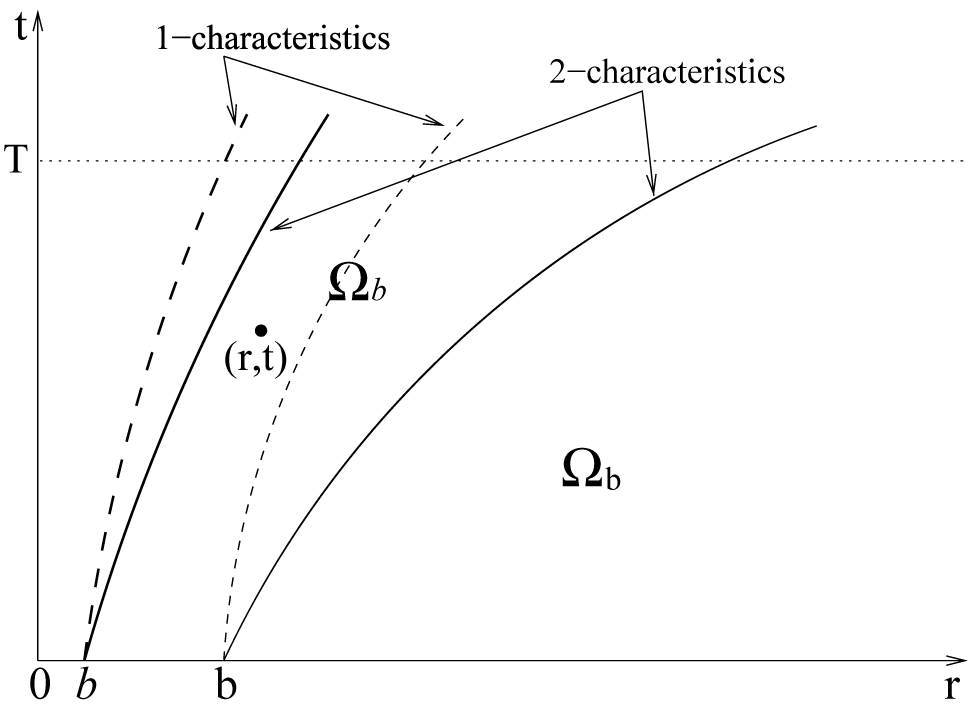
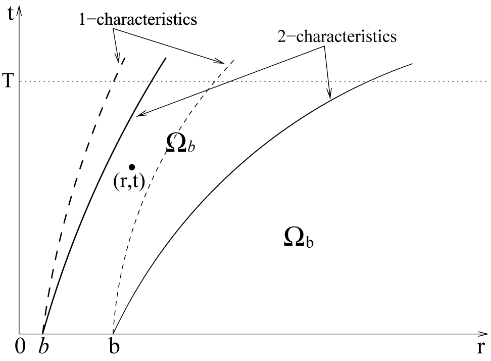
(see Figure 2 for illustration). To show this assertion, it is only necessary to verify that the characteristic starting from
 $(r,t)=(0,0)$
must be
 $r=0$
. We also use the contradiction argument to demonstrate it. Assume that, without loss of generality, the
 $2$
-characteristic
 $r=\tilde {r}(t)$
starting from the point
 $(r,t)=(0,0)$
goes away from
 $r=0$
at
 $t=\check {t}$
, that is,
 $\tilde {r}(\check {t})=0$
and
 $\tilde {r}(t)>0$
when
 $\check {t}<t<\check {t}+\bar {\delta }$
, where
 $\bar {\delta }$
is a small positive number. And we only consider smooth solutions before gradient blowup on
 $r=\tilde {r}(t)$
with
 $\check {t}\leq t\leq \hat {t}<\check {t}+\bar {\delta }$
. According to the differential mean value theorem with respect to r, it suggests that
 $$ \begin{align} \lambda_2(r,t)=\lambda_2(r,t)-\lambda_2(0,t)\leq \widetilde{K}r, \end{align} $$
for some positive constant
 $\widetilde {K}$
. Then, we see that on
 $r=\tilde {r}(t)$
 $$ \begin{align} \frac{\mathrm{d}\tilde{r}(t)}{\mathrm{d}t}=\lambda_2\leq \widetilde{K}\tilde{r}(t), \end{align} $$
from which one has
 $$ \begin{align} \tilde{r}(\hat{t})\leq e^{\widetilde{K}(\hat{t}-\check{t})}\tilde{r}(\check{t})=0, \end{align} $$
which contradicts to the fact
 $\tilde {r}(\hat {t})>0$
. Therefore, the characteristic starting from
 $(r,t)=(0,0)$
must be
 $r=0$
. Hence, we obtain the smooth solution on the entire domain
 $r\geq 0$
,
 $t\geq 0$
. The properties of solution in (2.12) and (2.13) follow directly by Theorem 5.1. The proof of Theorem 2.1 is complete.
The regions
 $\Omega _{\mathrm {b}}$
and
 $\Omega _{\mathrm {b}}$
.
6 Singularity formation
In this section, we present the proof of Theorem 2.2, that is, the singularity forms in finite time when the compressive initial data include strong compression somewhere.
We first establish the invariant domain for the compressive initial data.
Lemma 6.1 Consider a smooth solution of (1.4) with (1.2) on
 $\Omega _b\cap \{t\leq T_0 \}$
, satisfying Assumption 1 on
 $(b,\infty )$
with
 $b>0$
. We further assume that the functions
 $\alpha _0(r)$
and
 $\beta _0(r)$
fulfill (2.14), that is, they are compressed. Then, the smooth solution satisfies
 $$ \begin{align} \alpha(r,t)\leq0,\quad \beta(r,t)\leq0, \quad \forall\ (r,t)\in \Omega_b\cap\{t\leq T_0\}. \end{align} $$
Proof We note that the inequality (4.21) still holds now by the fact that the proof of Lemmas 4.1 and 4.2 only needs to use Assumption 1. Let
 $K_b$
and
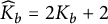 $\widehat {K}_b=2K_b+2$
be the constants defined in (4.21) and (4.22), respectively, and
 $\eta>0$
be a small number. We introduce two new variables
 $$ \begin{align} \widetilde{X}=\alpha+\eta e^{-\widehat{K}_b t}, \quad \widetilde{Y}=\beta+\eta e^{-\widehat{K}_b t}. \end{align} $$
Let
 $R>b$
be any fixed real number. Denote
 $$ \begin{align} \kappa_R=-\max_{r\in[b,R]}\{\alpha_0(r),\ \beta_0(r)\}. \end{align} $$
According to (2.14), we know that the number
 $\kappa _R$
is a positive constant. Now, we choose
 $\eta $
small enough such that
 $$ \begin{align} \eta\leq\min\bigg\{\kappa_R, \frac{16-(3-\gamma)^2}{16}\bigg\}. \end{align} $$
Thus, it follows by (6.2)–(6.4) that
 $$ \begin{align} \widetilde{X}(r,0)<0,\ \widetilde{Y}(r,0)<0,\quad \forall\ r\in[b,R]. \end{align} $$
Moreover, in view of Lemma 3.1, we can obtain the governing system of
 $(\widetilde {X}, \widetilde {Y})$
as follows:
 $$ \begin{equation} \begin{aligned}\partial_2\widetilde{X}&=\bigg\{-\frac{1-\varepsilon u^2}{(1+\varepsilon au)^2}\frac{(\gamma+1)(\gamma-\varepsilon a^2)}{4\gamma}(\widetilde{X}-2\eta e^{-\widehat{K}_b t}) \\ &\quad -\frac{1-\varepsilon u^2}{(1+\varepsilon au)^2}\frac{\gamma(3-\gamma)+\varepsilon a^2(1-3\gamma)}{4\gamma}(\widetilde{Y}-\eta e^{-\widehat{K}_b t}) -B_2\bigg\}\widetilde{X} \\ &\quad +\bigg\{\frac{1-\varepsilon u^2}{(1+\varepsilon au)^2}\frac{\gamma(3-\gamma)+\varepsilon a^2(1-3\gamma)}{4\gamma}\eta e^{-\widehat{K}_b t}+A_2\bigg\}\widetilde{Y} \\ &\quad -\eta e^{-\widehat{K}_b t}\bigg\{\widehat{K}_b+A_2-B_2+\frac{(1-\varepsilon u^2)(1-\varepsilon a^2)}{(1+\varepsilon au)^2}\eta e^{-\widehat{K}_b t}\bigg\}, \end{aligned}\end{equation} $$
and
 $$ \begin{equation} \begin{aligned}\partial_1\widetilde{Y}&=\bigg\{-\frac{1-\varepsilon u^2}{(1-\varepsilon au)^2}\frac{(\gamma+1)(\gamma-\varepsilon a^2)}{4\gamma}(\widetilde{Y}-2\eta e^{-\widehat{K}_b t}) \\ &\quad -\frac{1-\varepsilon u^2}{(1-\varepsilon au)^2}\frac{\gamma(3-\gamma)+\varepsilon a^2(1-3\gamma)}{4\gamma}(\widetilde{X}-\eta e^{-\widehat{K}_b t}) -B_1\bigg\}\widetilde{Y} \\ &\quad +\bigg\{\frac{1-\varepsilon u^2}{(1-\varepsilon au)^2}\frac{\gamma(3-\gamma)+\varepsilon a^2(1-3\gamma)}{4\gamma}\eta e^{-\widehat{K}_b t}+A_1\bigg\}\widetilde{X} \\ &\quad -\eta e^{-\widehat{K}_b t}\bigg\{\widehat{K}_b+A_1-B_1+\frac{(1-\varepsilon u^2)(1-\varepsilon a^2)}{(1-\varepsilon au)^2}\eta e^{-\widehat{K}_b t}\bigg\}. \end{aligned}\end{equation} $$
We first consider the smooth solution in the region
 $\Omega _b\cap \{(r,t)|\ r\leq R,\ t\leq T_0 \}$
. If
 $(\bar {r},\bar {t})\in \Omega _b\cap \{(r,t)|\ r\leq R,\ t\leq T_0 \}$
is the first time such that
 $\widetilde {X}(\bar {r},\bar {t})=0, \widetilde {Y}(\bar {r},\bar {t})\leq 0$
, then one has
 $$ \begin{align} \partial_2\widetilde{X}|_{(\bar{r},\bar{t})}\geq0. \end{align} $$
On the other hand, we observe from (6.6) that
 $$ \begin{align} &\partial_2\widetilde{X}|_{(\bar{r},\bar{t})} \nonumber\\ &\quad \leq -\eta e^{-\widehat{K}_b t}\bigg\{\widehat{K}_b+A_2-B_2+\frac{(1-\varepsilon u^2)(1-\varepsilon a^2)}{(1+\varepsilon au)^2}\eta e^{-\widehat{K}_b t}\bigg\}<0, \end{align} $$
by (4.25). This yields a contradiction. If
 $(\bar {r},\bar {t})\in \Omega _b\cap \{(r,t)|\ r\leq R,\ t\leq T_0 \}$
is the first time such that
 $\widetilde {X}(\bar {r},\bar {t})\leq 0, \widetilde {Y}(\bar {r},\bar {t})=0$
, the proof is similar. Thus, we have
 $$ \begin{align} \widetilde{X}(r,t)<0,\ \widetilde{Y}(r,t)<0,\quad \forall\ (r,t)\in\Omega_b\cap\{(r,t)|\ r\leq R,\ t\leq T_0 \}, \end{align} $$
and subsequently
 $$ \begin{align} \alpha(r,t)<-\eta e^{-\widehat{K}_b t}<0,\quad \beta(r,t)<-\eta e^{-\widehat{K}_b t}<0, \end{align} $$
for any
 $(r,t)\in \Omega _b\cap \{(r,t)|\ r\leq R,\ t\leq T_0 \}$
. Due to the arbitrariness of R, we obtain
 $$ \begin{align} \alpha(r,t)\leq0,\ \beta(r,t)\leq0,\quad \forall\ (r,t)\in\Omega_b\cap\{t\leq T_0 \}. \end{align} $$
The proof of the lemma is complete.
To proceed, we need to derive an only time-dependent density positive lower bound in the current conditions.
Lemma 6.2 Let the assumptions in Lemma 6.1 hold. Moreover, suppose that (4.32) holds, that is,
 $\underline {\rho }=\min _{r\in [b,\infty )}\rho (r,0)>0$
. Then, the smooth solution satisfies
 $$ \begin{align} \rho(r,t)\geq \underline{\rho} \Big(\frac{4b\sqrt{\varepsilon}}{4b\sqrt{\varepsilon}+(3-\gamma)t}\Big)^{d-1} e^{-\widetilde{M}_bt}, \end{align} $$
for
 $(r,t)\in \Omega _b\cap \{t\leq T_0\}$
, where
 $$ \begin{align} \widetilde{M}_b=\frac{(d-1)(\gamma^2-1)(\sqrt{2}+\sqrt{\gamma+1})}{4b\gamma\sqrt{2\varepsilon}}. \end{align} $$
Proof Recalling the first inequality in (4.41), we have by (6.1) and (6.14)
 $$ \begin{align} \partial_0\ln\Big(\frac{1}{r^{d-1}\rho}\Big)\leq \frac{(d-1)(\gamma^2-1)(\sqrt{2}+\sqrt{\gamma+1})}{4b\gamma\sqrt{2\varepsilon}}+\beta+\alpha \leq \widetilde{M}_b. \end{align} $$
Recalling the definition of the curve
 $r=r_0(t)$
in (4.42) and using the estimate (4.44), we integrate (6.15) along
 $r=r_0(t)$
to obtain
 $$ \begin{align} \rho(r,t)\geq& \Big(\frac{r_0(t_0)}{r_0(t)}\Big)^{d-1}\rho_0(r_0)e^{-\widetilde{M}_bt} \nonumber \\ \geq& \underline{\rho} \Big(\frac{4b\sqrt{\varepsilon}}{4b\sqrt{\varepsilon}+(3-\gamma)t}\Big)^{d-1} e^{-\widetilde{M}_bt}, \end{align} $$
for any
 $(r,t)\in \Omega _b\cap \{t\leq T_0\}$
. The proof of the lemma is completed.
Proof of Theorem 2.2.
Now, we are going to show Theorem 2.2. Recalling the coefficients of
 $\beta ^2$
and
 $\alpha ^2$
in (3.5) and (3.7), respectively, one has by (4.19)
 $$ \begin{align} &-\frac{1-\varepsilon u^2}{(1\pm\varepsilon au)^2}\frac{(\gamma+1)(\gamma-\varepsilon a^2)}{4\gamma} \nonumber \\ \leq& -\frac{16-(3-\gamma)^2}{2^2\cdot 16} \cdot\frac{\gamma-1}{4}=-\frac{(\gamma-1)[16-(3-\gamma)^2]}{256}, \end{align} $$
which, together with Lemmas 3.1, 6.1, and 6.2, yields
 $$ \begin{equation} \begin{aligned}&\partial_1\beta\leq-\frac{(\gamma-1)[16-(3-\gamma)^2]}{256}\beta^2 -K_b\beta \\ &=-\frac{(\gamma-1)[16-(3-\gamma)^2]}{512}\beta^2 -\Big(\frac{(\gamma-1)[16-(3-\gamma)^2]}{512}\beta+K_b\Big)\beta, \\ &\quad \partial_2\alpha\leq-\frac{(\gamma-1)[16-(3-\gamma)^2]}{256}\alpha^2-K_b\alpha \\ &=-\frac{(\gamma-1)[16-(3-\gamma)^2]}{512}\alpha^2 -\Big(\frac{(\gamma-1)[16-(3-\gamma)^2]}{512}\alpha+K_b\Big)\alpha. \end{aligned}\end{equation} $$
Set
 $$ \begin{align} N(b,T)=\max\bigg\{\frac{512K_b}{(\gamma-1)[16-(3-\gamma)^2]},\frac{512}{(\gamma-1)[16-(3-\gamma)^2]T}\bigg\}. \end{align} $$
If
 $\alpha _0(r^*)\leq -N(b, T)$
, we consider the 2-characteristic curve
 $r=r_2(t; r^*,0)$
for
 $t\in [0,T)$
to observe that
 $$ \begin{align*}\frac{(\gamma-1)[16-(3-\gamma)^2]}{512}\alpha(r_2(t; r^*,0),t)+K_b\leq0, \end{align*} $$
and then
 $$ \begin{align} \partial_2\alpha\leq -\frac{(\gamma-1)[16-(3-\gamma)^2]}{512}\alpha^2, \end{align} $$
along
 $r=r_2(t; r^*,0)$
. Integrating (6.20) yields
 $$ \begin{align} \frac{1}{-\alpha(r,t)}\leq \frac{1}{-\alpha_0(r^*)} -\frac{(\gamma-1)[16-(3-\gamma)^2]}{512}t, \end{align} $$
which implies that blowup happens not later than
 $$ \begin{align} T^*=\frac{512}{-\alpha_0(r^*)(\gamma-1)[16-(3-\gamma)^2]}\leq T. \end{align} $$
If
 $\beta _0(r^*)\leq -N(b,T)$
at some point
 $r^*$
, we can similarly show the blowup time is before
 $T^*$
. The proof of Theorem 2.2 is complete.
Acknowledgements
The authors would like to thank the anonymous reviewer for very helpful comments and suggestions to improve the quality of the article.