

On 21 March 2010, members of the House of Representatives cast votes that shaped American politics for the rest of the decade.Footnote 1 The bill in question, the Patient Protection and Affordable Care Act (“ACA”), offered the most significant changes to American healthcare policy in decades. The 21 March vote had an air of finality; a mixture of electoral and procedural circumstances meant that the bill could not be modified further.Footnote 2 Pass and the bill would go to President Barack Obama and become law; fail and “Obamacare” would go back to the drawing board to become a much smaller programme. Facing a pivotal choice on the path of American health insurance policy, a sufficient number of moderate Democrats voted for passage and the bill became law. As a result, significant policy changes were set in motion in the American healthcare system. The question of the wisdom of the ACA would be one of the central axes of ideological and partisan conflict for the next decade.Footnote 3
Less than a year later, on 19 January 2011, members of the now-Republican-majority House again faced a roll call on the ACA – this time on its wholesale repeal.Footnote 4 However, there was something missing in the 19 January vote: any possibility for policy change. The Senate remained under Democratic control, and President Obama held his veto pen ready. Obamacare was not going to be repealed. The best hope of reversing the policy was with the conservative-leaning US Supreme Court. Nevertheless, the House voted to “repeal” the ACA. In total, the Republican-majority House would repeal the ACA roughly once every six weeks over the last six years of the Obama Administration. But the dozens of these votes had less combined policy significance than the single pivotal March 2010 vote (O’Keefe Reference O’Keefe2014).Footnote 5
The frequently confounding story of the House roll calls on the ACA raises several interesting substantive and methodological questions about the study of voting in Congress. The first is the difference between votes as messages and votes as policy. Mayhew (Reference Mayhew1974), among others, has argued that members take positions, and they do not systematically seek policy. The policy consequences of a vote – distant and uncertain – are less important than the message of the vote, which can redound to the member’s popularity immediately.Footnote 6 This implies that there should be little difference between votes that have policy implications (such as the March 2010 ACA vote) and those that do not (such as the many symbolic votes during divided government that followed). The method of vote choice is the same: the message is the point. This is in stark contrast with many existing formal theoretical approaches to voting in Congress, which heavily rely on actual policy as the driving force in voting.
On a methodological level, the answer to this question is consequential. Our dominant approaches to measuring member ideology rely on evaluating aggregated votes. But the accumulation of all votes necessarily captures many votes with no policy consequences at all. The underlying formal logic of these measurement models is a spatial policy vote choice game, but many (even most) votes will not implicate policy. If the methods of vote choice are not constant across votes regardless of their policy implications, then the inclusion of these votes in measurement models may bias our estimates. This could lead, for example, to overestimating partisan ideological polarisation by inflating measures with numerous “meaningless” votes – such as the many dozens of ACA-repeal votes, which for symbolic reasons tended to perfectly divide the parties.
We evaluate this question by separating all roll calls during the four Obama Administration Congresses (the 111th – 114th) into two bins: those with a clear possibility of becoming law – which we call “credible policy votes” – and those without. We perform two comparisons, one for a substantive point and one for a methodological point. First, we compare the ideal point estimates obtained using just the credible policy votes to estimates obtained using just the noncredible votes. What we find largely supports a Mayhewian perspective: members appear to approach both credible and noncredible votes (in terms of policy impacts) in substantially the same way. The policy outcome may not matter that much next to being seen voting for the right policy. Though we find and analyse some minor differences, the overall relationship is considerable similarity.
Second, we evaluate the methodological question of whether common measurement systems are biased by their use of noncredible votes. To do this, we compare the measures obtained from the credible votes to those obtained using all votes. Here again, we find minimal differences, implying that using data sets comprised of all votes does not introduce material bias to political science research in most cases.
To assess whether this finding may be an artefact of the modern, highly polarised Congress, we perform the same task on all roll calls during the four Eisenhower Administration Congresses (the 83rd – 86th), a time when both parties were significantly more heterogeneous. We find essentially the same results as during the Obama Administration. Finally, though our results largely support the continued use of the leading measurement systems in the field, they do raise questions about the importance of “policy” in the way ideal points are typically described and framed. Rather than “revealed” spatial policy preferences, ideal points may better reflect preferences over available positions to take.
The importance of policy in Congressional voting
Conventional models of voting in Congress assume that members have utility functions over specific policy outcomes. It is commonly assumed that the set of outcomes for a voting action is a line of possible policies.Footnote 7 Spatial utility logic provides a specific functional form to the simple idea that members will pick the option most similar to their ideal policy. Voting games – such as Pivotal Politics (Krehbiel Reference Krehbiel1998) – rely on each member having a preference over policy outcomes that spatially dictates their vote on any given roll call. These theoretical approaches assume that the sole mechanism of voting choice is spatial proximity over policy. The preferences may derive from a host of different sources – induced by elections through voters or donors, induced by the demands of party membership, or perhaps the durable personal principles of the legislator – but they are about policy outcomes.
A similar spatial utility framework underlies measurement models of legislator preferences – for example, in the Item Response Theory (IRT) framework of Jackman (Reference Jackman2001) and Clinton et al. (Reference Clinton, Jackman and Rivers2004), or the NOMINATE system by Poole and Rosenthal (Reference Poole and Rosenthal1997, Reference Poole and Rosenthal2007) and Poole (Reference Poole2005). The IRT framework, for example, is an expression of the standard spatial utility voting model, which happens to be equivalent to a popular model of educational testing evaluation. These models assume a shared space of policy over which members have varying ideal points.
Despite the exclusive focus on policy in the canonical models, the reality of Congress is often quite different. One key aspect of Congressional voting is that everyone gets the same policy in the end. If the proposal passes, all members get the proposed policy. And most times, when the proposal fails, that policy is just yesterday’s policy continued forward. The status quo dominates. Members are not given a choice to take the policy they like between two options. They, and the rest of the country, get whatever wins. Though they may take hundreds, or more than a thousand, roll calls in a year, members of Congress produce relatively little policy change, as evidenced by the number of significant enactments (Mayhew Reference Mayhew2005; Stathis Reference Stathis2014). Many policies are simply impossible to pass given the arrangement of veto players (Krehbiel Reference Krehbiel1998; Gray and Jenkins Reference Gray and Jenkins2019). This means that much of the time, members are casting votes on things that will result in little or no policy change. When the “game” is over, each receives the same policy – the current policy – and this outcome is known in advance, as votes are only allowed to come to the floor when leadership’s desired outcome will be reached.
This does not provide a natural fit with the benchmark models that both underlie our theoretical explanations of Congress but also our measurement models that produce preference estimates used across thousands of research projects in political science. Despite being about choosing between policies, most votes do not involve a policy choice at all. Policy differences cannot be a mechanism for deciding vote outcomes when there is no policy change no matter how the member votes. It is easy to fill in nonpolicy motivations for voting: position-taking or “messaging” and maintaining a consistent platform. Yet these are not part of the benchmark models nor of the measurement models, which utilise thousands of votes that must ultimately rely on these other considerations.
This raises several interesting possibilities. One is that members might have different voting approaches: one when policy may be credibly changed by a vote choice and one when it may not. This would imply two different data-generating processes and pose difficult questions about measurement models that bunch all votes together. It is possible that true “policy preferences” are obscured by thousands of symbolic and noncredible votes that are driven by a different voting calculus. This could lead to biases, potentially over- or under-estimating concepts of interest such as partisan polarisation. Existing work by Theriault (Reference Theriault2008) and Jessee and Theriault (Reference Jessee and Theriault2014) suggests that partisan polarisation is overestimated by the inclusion of procedural votes, which lack policy content, and on which parties act cohesively. It is possible that even on substantive votes, many of them have no possible variation in policy outcome and thus rely on a different data-generating process.
Alternatively, it is possible that policy was never that important to begin with. Perhaps the act of voting is what members care about. In this conception, they vote similarly regardless of whether the vote credibly could change policy, because they want to be observed taking positions on things, regardless of whether they ever come to be. Mayhew (Reference Mayhew1974, 62) provides a possible basis for this type of outcome-agnostic voting: “The Congressman as position taker is a speaker rather than a doer. The electoral requirement is not that he makes pleasing things happen but that he makes pleasing judgmental statements. The position itself is the political commodity.”Footnote 8 More than forty years later, Frances Lee (Reference Lee2016, 12) echoed this argument: “Leaders and members regularly set up roll call votes in full knowledge that these votes will have no effect on policy outcomes, but they nevertheless stage them for messaging purposes.”
Position taking is a well-used concept in the study of American politics. Indeed, some votes are colloquially called “messaging votes” or “position-taking votes,” as it is accepted that their sole value is to message to their voters by taking a position on a vote – or to force the opposition to take a position – with no actual policy consequences for anyone. For example, in the last Republican-controlled Senate, then Republican Majority Leader Mitch McConnell (KY) brought up a vote on a resolution on the “Green New Deal,” which he opposed, because he knew that it would fail and sought to put Democrats “on the spot” – and require them to take a position on the unpopular proposal. The idea that some votes are meant solely for messaging purposes has been admitted by some members of Congress – including Speaker Nancy Pelosi (R-CA) – and has been included more and more in journalistic accounts of Congressional behaviour (Kiefer Reference Kiefer2015; Becker Reference Becker2018; McPherson 2018; Reference McPherson2019). “Messaging votes” even have their own entry in the index of Mitch McConnell’s (Reference McConnell2016) memoir.
The question remains whether a member’s utility function for votes of this type is the same as the utility function for votes when the policy is actually up for change. If they are different, this would suggest necessary changes or qualifications on existing approaches to estimation of policy preferences, as those measures would be mixing data from two different situations, relying on two different utility functions. If they are the same, it implies the usefulness of those measures, but would also raise questions as to how we frame those measures.
Empirical analysis
We test whether there is evidence of two different approaches to voting depending on the credibility of policy change resulting from a vote. To do this, we separate out votes where there was a credible chance of a policy change resulting from that vote. We focus on the four Congresses of the Obama presidency and estimate ideal points on these votes, which we call the “Policy Set.” Our two separate ways of looking at this question – substantively and methodologically – necessitate two comparisons. First, we compare ideal point estimates on this Policy Set to the same type of estimation on the remaining votes deemed noncredible, which we call the “Non-Policy Set.” If the possibility of policy change induces a different voting calculus or relies on a different utility function, we should observe different results between the Policy and Non-Policy Sets. Second, we compare the estimates from the Policy Set to the estimates we would get in an estimation on all of the votes from these four Congresses, which we call the Full Set. We find minimal differences in the House and among Senate Democrats and modest differences in the Senate among Republicans. In total, our findings imply a highly similar voting calculus for members regardless of the policy stakes in a vote. This gives empirical weight to Mayhew’s assertions that the position itself is the political commodity, not the policy outcome.
Defining a “credible” vote
We separate all votes into two categories: those with a credible chance to change policy and those that are noncredible as policy changes. Separating roll calls into categories and analysing (or scaling) them independently is not new, of course. Others, for example, have split procedural votes from policy votes (Theriault Reference Theriault2008; Jessee and Theriault 2014), close votes from lopsided votes (Snyder and Groseclose Reference Snyder and Groseclose2000), amendment votes from others (Roberts and Smith Reference Roberts and Smith2003) and votes in some policy domains from others (Clausen Reference Clausen1973; Peltzman Reference Peltzman1984; Poole and Rosenthal Reference Poole and Rosenthal1997). And, in general, concerns over the composition of the roll call record have animated research for decades. Our question is also concerned with the composition of roll calls, but we seek a new differentiation: final passage votes on policies that also had a meaningful likelihood of being passed. This removes procedural and amendment votes, but also removes policy votes on bills with minimal likelihood of passing. We wish to recover the set of votes that were taken with the real pressure of possibly changing the law in the United States (US).
Our approach of producing two bins (“credible” and “noncredible”) of votes is an admitted dichotomous simplification over an unobserved continuous dimension of likelihood of becoming law. We accomplish this categorisation by creating a set of coding rules based exclusively on before-the-vote information. For each arrangement of political power, we create a different set of coding rules. The Obama Administration provides an interesting period for testing because it contains all of the relevant divisions of power. In the first Congress (the 111th), Democrats enjoyed first filibuster-proof unified control followed by filibuster-constrained unified control of government. In the two middle Congresses (the 112th and 113th), Democrats controlled the Presidency and the Senate, but not the House. Finally, in the 114th Congress, Republicans had unified control of Congress, while Democrats retained the Presidency.Footnote 9
As an initial matter, we consider only “passage votes” as possibly being credible policy votes. These include votes on passage within a chamber, votes agreeing in full in amendments of another chamber and conference committee report votes. This removes all procedural and amendment votes from consideration. Procedural votes do not always have direct policy implications. One can vote for cloture but against a bill. Similarly, amendments themselves do not change policy. Many are attached to bills of little consequence and thus are themselves of little consequence. When they are consequential, they are also included in the final passage roll call.
Additionally, we exclude all bills with nonmajority vote requirements. These bills present different calculations because of their higher threshold for passage. Thus, we do not consider the (few) votes on veto overrides during the Obama Administration. We also do not consider passage votes taken under a “suspend the rules and agree” question. In total, this leaves 1737 majority passage votes combined for the two chambers across four Congresses.
Our classification approach is to rely on existing facts at the time of a vote to predict the likelihood that the vote is credible to pass. We assume as a starting matter that there is a set of bills that are credible to pass regardless of the political distribution: “must-pass” legislation. These bills include annual appropriations bills, continuing funding bills, debt ceiling increases, as well as emergency bills and disaster-response bills. Though they may be subject to significant partisan fighting, these are bills that Congress must – and does – pass regardless of who is in control and thus when they are brought to the floor are credible to pass and become policy.
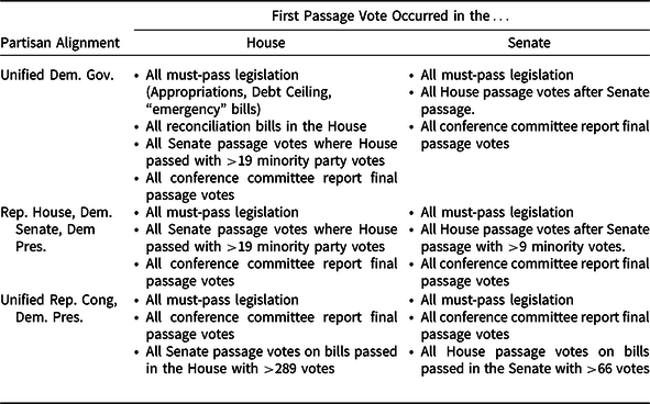
Unsurprisingly, we assume that votes advanced during periods of unified government are more likely to become law than those advanced during divided government. In general, we wish to include votes where the existing political arrangement or previous legislative action on a bill points to a possibility of success. We assume that some evidence of bipartisanship is required to predict success during the periods where Congress is split between the two parties. We rely on the fact that votes happen in sequence with one chamber going before the other. When a bill passes in the House, we can say something when it comes up in the Senate based on how the House minority (which is the Senate majority party) voted on the bill. Thus, for example, a bill that passes in the House with zero support from Democrats does not have high hopes in the Democrat-controlled Senate. However, a bill that passes first in the House with significant bipartisan support implies a real possibility in the Senate. Specifically, we choose bills receiving at least ten minority party votes in the Senate or 20 minority party votes in the House as those where sufficient bipartisanship was possible for the bill to pass the second chamber.Footnote 10 Once a bill has reached the conference committee stage, we assume its passage is credible. We list the technical coding rules for each arrangement of political power in Table 1. Of the 1737 majority-rule passage votes, we retain 582 as credible: 426 in the House and 156 in the Senate.
Roll-call classification rules

Because we analyse only four Congresses, with only a few members changing between chambers, and relatively few votes, we do not attempt to create “Common Space” scores. Instead, we estimate individual chamber-specific scores for the combined eight-year period. As is conventional, this relies on continuing membership across Congresses to “bridge.” Specifically, we estimate conventional single-dimension, two-parameter (IRT) models in which each roll call is treated as an item or “question” (Martin et al. Reference Martin, Quinn and Park2011). The model estimates a difficulty parameter and discrimination parameter for each roll call along with an ability level for each voter. In this case, ability levels are interpreted as “ideal points,” increasing in conservatism.
Results
Do members vote similarly on credible and noncredible votes?
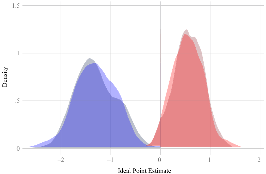
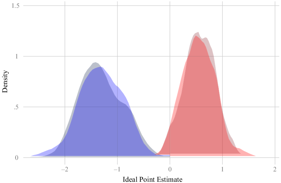
In each of the following figures, we compare the results obtained using conventional one-dimensional IRT models on the Credible Set of votes with credible policy implications and the Non-Credible Set of all remaining votes. As the models are estimated separately on the House and the Senate and the results are not comparable, we analyse each individually. We first explore the results in the House. In Figure 1, we present the distributions of DemocratsFootnote 11 and Republicans with both the Credible Set and the Non-Credible Set.
Comparison of partisan distributions in the House for the Credible (Lighter) and Non-Credible (Darker) Sets of roll calls, 111th to 114th Congresses.

We can only describe this result as remarkable similarity. Estimates based on votes that might credibly impact policy return almost identical distributions of Republicans and Democrats as measures based only on votes that are unlikely to impact policy. Labels are hardly even necessary in the figure given their substantial similarities. Unsurprisingly, in a Kolmogorov-Smirnov (K-S) difference of distributions test, we are unable to reject the null that they are both derived from the same distribution. This is one first piece of evidence in favour of the perspectives offered by Mayhew and Lee: behaviour on things totally unrelated to policy – like messaging and partisan procedural games – produce the same apparent preference distribution as policy votes. The correlation between the two is 0.97.
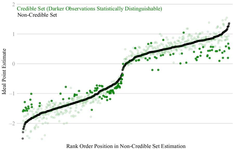
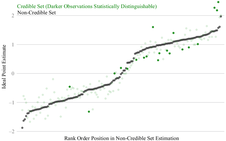
Changes in partisan distributions may be difficult to capture among so many votes. We next move to analysing individual changes in the House, which we present in Figure 2. We compare the estimates derived from the Non-Credible Set to those in the Credible Set, which are labelled in green. We darken estimates that are statistically distinguishable and lighten those that are not. We find some interesting visual patterns, but an overall trend of similarity that matches the partisan distributions. Most members receive similar scores from both estimates. Notably, many that are statistically distinguishable, and almost all such Republicans, are in a moderating direction. That is, noncredible votes make them appear more extreme than credible votes would. This accords with existing work, such as that by Theriault (Reference Theriault2008). Notably, however, we do not find that this is a material and systematic problem. Because we rely on estimates with reduced sets of votes, we must be mindful of the power of our analysis: it is possible that large standard errors mean that large differences are not statistically distinguishable. Yet that is not a problem in our analysis. About 75% of legislators are measured with sufficient precision in each set such that we could statistically detect differences of half a chamber standard deviation (0.5 in the ideal point scale). Nearly every legislator would be detectable with a gap over one standard deviation. As we see in Figure 2, such large differences between revealed preferences in the two sets are rare, and we usually measure them with sufficient precision. Given more data, we could obtain more precise measures, but these would not change our conclusions.
Individual representative scores in Policy Set (Green) overlaid on scores in Non-Policy Set (Black).

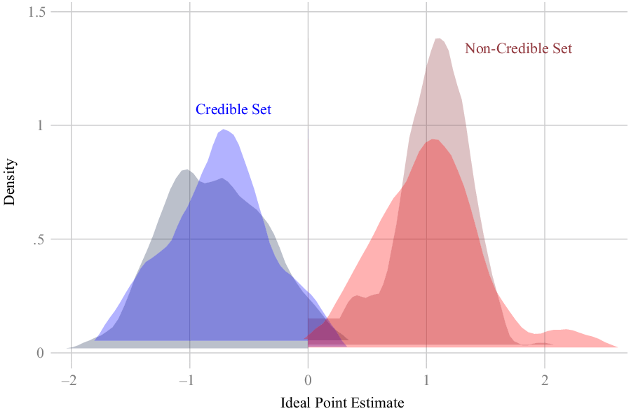
In Figures 3 and 4, we present analogous data to Figures 1 and 2, except for the Senate. First, in Figure 3, we find a less striking level of similarity for Senators. While Democrats provide the type of similarity found in the House, there are differences in the Senate, where Republicans appear more unified in the Non-Credible Set than in the Credible Set. However, even with these differences, we are still unable to reject the null in a K-S test of a common underlying distribution. The correlation between the two types of scores is 0.96. The overall correlation combining the House and the Senate is 0.97.
Comparison of partisan distributions in the Senate for the Policy (Lighter) and Non-Policy (Darker) Sets of roll calls, 111th – 114th Congresses.

Individual Senator Scores in Policy Set (Green) overlaid on scores in Non-Policy Set (Black).

In Figure 4, we find few Senators that have substantially different estimates between the two different vote sets, and relatively few with a statistically significant difference, almost all of which are Republicans. This is in keeping with Figure 3 and the unique nature of Senate Republicans among the four groups we analyse in this article. When analysed in the Non-Credible Set, Republicans seem relatively homogenous, centred around a conservative position almost exactly one standard deviation to the right of the chamber mean. However, when only looking at credible policy votes, the Republican Party appears much more varied in the Senate, with more moderate and more extreme members. In this telling, there is no apparent difference between a moderate Republican such as Susan Collins (ME) and a moderate Democrat such as Ben Nelson (NE). Meanwhile, there is a much greater difference between a moderate like Collins and one of the party’s most conservative members, such as Mike Lee (UT).
One possible explanation for Senate Republicans as the sole meaningful difference is the particular strategy adopted by Senate Majority Leader Mitch McConnell during the Obama Administration. Senator McConnell’s publicly admitted strategy was constant obstruction. He marshalled his party to constantly obstruct policy change, especially during the six years in the minority until 2015. On many of these votes, Senator McConnell was effective in holding partisan unity in a way that may yield the more homogenous results such as those in Figure 3. Ultimately, however, when policy was on the line in final passage votes, his members showed their variation. More moderate members were more likely to participate in compromise legislation with the Administration, while his more extreme flank was less willing to do so. The difference in results between the Non-Credible and Credible Sets may be evidence of McConnell’s leadership success during the Obama Administration. In sum, we find considerable similarity between estimates derived from credible and noncredible votes. This is true for both parties in the House, the Democrats in the Senate, and somewhat less so for Senate Republicans. This further strengthens the evidence that policy may not be the key driving factor of decisions, but rather the more political elements such as messaging and partisanship.
Are existing measurement systems biased by their inclusion of noncredible votes?
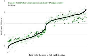
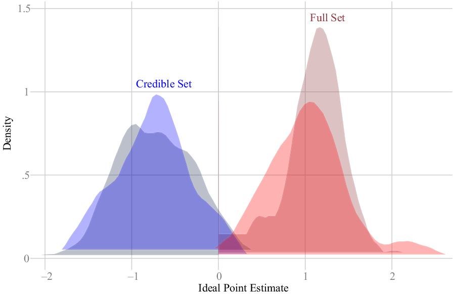
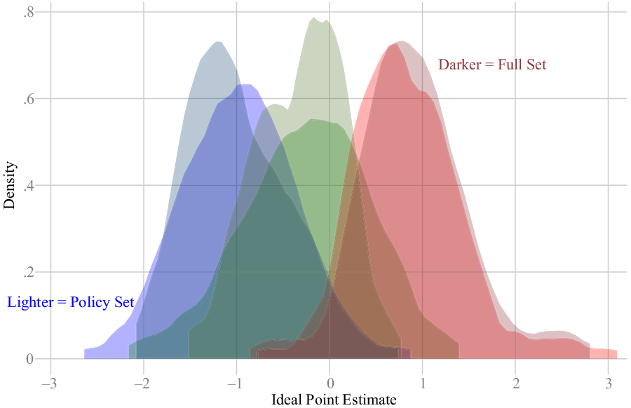
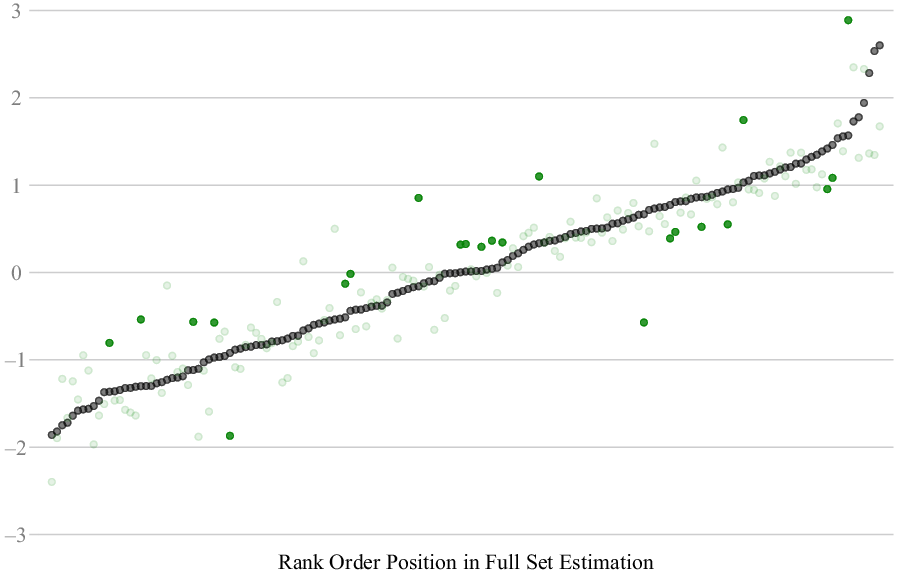
Given the results in the preceding section, concern over the potential bias in widely used measures of all votes should already be minimised. As the Full Set is overwhelmingly made up of Non-Policy votes, the results of the Non-Credible Set and the Full Set are nearly identical. Thus, given the similarity between the Credible Set and Non-Credible Set, the Credible Set is also very similar to the Full Set. The correlation between the two is 0.97. We do not belabour this point with repeated articulation and present Figures 5-8, replicating those in Figures 1-4, but with the alternative comparison. The results generally support the use of current Full Set-based measures.
Comparison of partisan distributions in the House for the Policy (Lighter) and Full (Darker) Sets of roll calls, 111th – 114th Congresses.

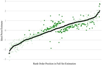
Individual representative scores in Policy Set (Green) Overlaid on Scores in Full Set (Black).

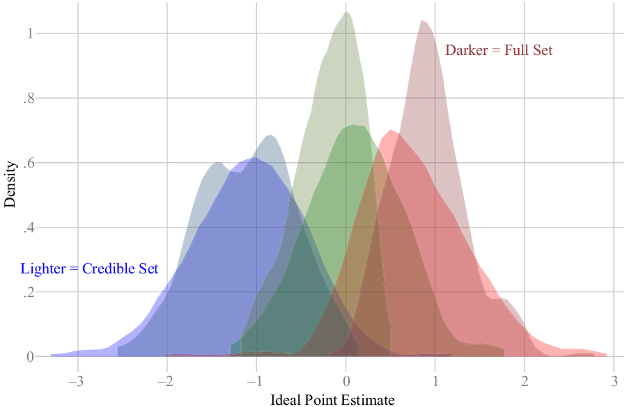
Comparison of partisan distributions in the Senate for the Policy (Lighter) and Full (Darker) Sets of roll calls, 111th –114th Congresses.

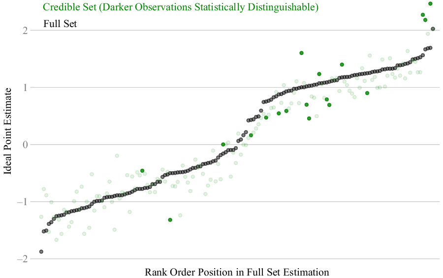
Individual Senator Scores in Policy Set (Green) Overlaid on Scores in Full Set (Black).

Partisan polarisation and unity
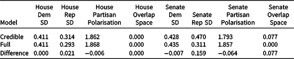
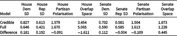
One possible concern of including many extra policy-meaningless votes is that if parties are better able to work as a team on these more symbolic bills, they may give an impression of a more unified party and more polarisation between parties. When policy-credible votes are taken, perhaps parties are more diverse and less different from each other. In Table 2, we present summary statistics on party unity, party overlap and party polarisation in the two chambers between the Policy and Full Sets. These values confirm the graphical results presented in Figures 1, 3, 5, and 7: the only meaningful difference is in the party homogeneity of Senate Republicans. In this, we observe a meaningful shift in moving to the credible set, with a much more dispersed party. In all other measurements of interest, we observe no material difference.
Summary statistics of partisan differences between credible and full set models

Note: “Partisan Polarisation” here is defined as the difference between the party means.
A replication in the Eisenhower Administration
One limitation of our primary analysis is that it focuses on a narrow eight-year period in a partisan environment distinct from much of modern US history. To address this, we replicate our approach on a very different partisan environment – the four Congresses of the Eisenhower Administration (the 83rd – 86th). During this period, the Democratic Party was intensely divided by region and both parties contained members of widely different ideological positions. Much like the Obama Administration, President Eisenhower enjoyed one Congress of unified government (the 83rd), followed by three of divided government. Thus, this period provides points of commonality with a significant deviation in levels of partisan cohesion.
We replicate our analysis as closely as possible to that outlined in the preceding section; however, we modify it, as necessary, for the different context. For example, the filibuster was seldom used during the time period, and thus, we do not assume that any sizable minority would stop any bill in the Senate. Otherwise, we follow the rules we built for the Obama Administration years, following the appropriate division of power between the White House and the chambers of Congress. In this case, the last six Eisenhower years best match the last two years of the Obama Administration. In total, we keep 393 roll calls as the Credible Set in the Eisenhower Years, out of a total of 621 final passage recorded roll calls: 207 in the House and 185 in the Senate.
First, in Figure 9, we present the distributions, by party, in the House. In light of the different context, we break Democrats into Southern and non-Southern versions, with Southern Democrats labelled as green. Following that, in Figure 10, we present individual comparisons between the two models, as in the preceding section.
Comparison of partisan distributions in the House for the Policy (Lighter) and Full (Darker) Sets of roll calls, 83rd to 86th Congresses.

Individual representative scores in Policy Set (Green) Overlaid on Scores in Full Set (Black).

In the House, we find some differences between the distributions, but not dramatic ones. Primarily, the Credible Set model implies that the Republicans and Southern Democrats voted more similarly on credible policy votes than we might expect from the full model. Despite this difference, neither party is significantly different from its Full Set model results. This pattern is also evidence in Figure 10, presenting the individual differences. The empty spaces below (left) and above (right) the centre show that moderate members were misestimated in a more extreme direction by the full model. Moderate liberals (in the Full Set) were more conservative on credible policy votes, while the opposite is true for moderate conservatives (in the Full Set). Extreme members based on all votes show no consistent pattern of deviation when moving to the Credible Set.
In Figures 11 and 12, we perform the same analyses on the Senate. Here we find evident similarity between the two different models. All three “parties” appear quite similar no matter whether measured in the Full Set of votes or the Credible Set. And among individual Senators, there are no clear patterns of divergence in one direction or another.
Comparison of partisan distributions in the Senate for the Policy (Lighter) and Full (Darker) Sets of roll calls, 83rd to 86th Congresses.

Individual Senator Scores in Credible Set (Green) overlaid on scores in Full Set (Black).

Finally, in Table 3, we present information analogous to Table 2, summarising key distribution and difference data between the Full and Credible Set models. Here we see larger differences than in the Obama years, especially in the House. Still, these differences are only sufficient to reject the null of no difference in a K-S test at the p < 0.10 level, and only in the House. Overall, we do not uncover material differences between the measures, but our results do indicate that some features of the ideological distribution may be inflated or deflated by the inclusion of noncredible votes.
Summary statistics of partisan differences between credible and full set models

Note: “Partisan Polarisation” here is defined as the difference between the party means.
Conclusion
Members of Congress cast numerous votes on things that will never become law. During divided government, large portions of each chamber’s time are spent on symbolic votes and measures that have little chance of changing federal policy. These are often understood as “positioning votes” or “messaging votes.” Yet, if these votes represented a wholly different data-generating process, it would raise questions about their use to estimate legislators’ policy preferences, for which they currently make up large a large share of the usable data.
We find that this concern is unfounded. While there are slight differences between models based on all votes and those based only on credible policy-changing votes, these differences prove to be immaterial. Members are frequently consistent in their positions regardless of whether that position could actually become law. This also fits with arguments of those such as Poole (Reference Poole2007) that members are remarkably consistent in their approach regardless of changing contexts that we might think should alter their behaviour (see Gray and Jenkins Reference Gray and Jenkins2020).
In sum, despite the increasing attention that messaging votes attract in the media, there do not appear to be great differences between member behaviour in “credible” votes and those in messaging votes and partisan procedural games. They are, in fact, “honest messengers.” This should alleviate some concern that the data that undergirds so much of the research on Congress is fundamentally flawed by the inclusion of thousands of votes of a fundamentally different nature.
Nevertheless, these results do raise challenging questions about why there is such similarity and what that says about the theoretical interpretations scholars have used to understand these data over time. It is possible that these measures are not about policy preferences, but rather about preferences for being observed casting certain types of votes described in policy terms but lacking real connection to the laws of the US. In this article, we show that ideal point measures are consistent measures of some ideal preference, but we must acknowledge that a variety of strongly correlated but different factors drive these preferences.
Acknowledgement
An earlier version of this paper was presented at the 2019 Annual Meeting of the Midwest Political Science Association in Chicago, IL.
Data availability statement
Replication materials are available in the Journal of Public Policy Dataverse at https://doi.org/10.7910/DVN/V2UDHZ.