



1 Introduction
With a fossil record dating to the Middle Cambrian (Cartwright et al. Reference Cartwright, Halgedahl, Hendricks, Jarrard, Marques, Collins and Lieberman2007), jellyfish are one of the earliest examples of an active motile, multi-cellular organism and provide a window into the origins of muscle driven swimming. Lacking an agonist–antagonist muscle pairing, jellyfish propulsion emerges from interactions between the active contraction of the swimming muscles, the passive elastic re-expansion of the bell, and the forces acting on the organism from the surrounding fluid (Demont & Gosline Reference Demont and Gosline1988b ; Megill Reference Megill2002; Megill, Gosline & Blake Reference Megill, Gosline and Blake2005; Hoover & Miller Reference Hoover and Miller2015). Jellyfish begin their swimming cycle by contracting their coronally oriented subumbrellar swimming muscles, which deform their bell and expel fluid from the inner cavity of the bell. The mesoglea, an extracellular matrix composed of fibres of a collagen-like protein, stores the potential elastic energy generated by contraction and drives re-expansion of the bell when the swimming muscles relax. Because the resting shape of the bell depends on the mesogleal matrix, jellyfish propulsion has been viewed as a process of active deformation and elastic recoil.
Recently, the wake structure generated during jellyfish swimming was found to be dependent upon the fineness ratio of the bell, which is the ratio of bell height to bell diameter. Prolate jellyfish, which have higher fineness ratios, use jet propulsion to generate thrust, whereas oblate jellyfish, with a lower fineness ratio, use a paddling mechanism that exploits the vortex rings generated during the expansion of the bell (Dabiri, Colin & Costello Reference Dabiri, Colin and Costello2007). This finding resolved the question of how jellyfish generate significant thrust at larger body sizes while maintaining only a monolayer of muscles (Daniel Reference Daniel1983; McHenry & Jed Reference McHenry and Jed2003; McHenry Reference McHenry2007). Dabiri et al. (Reference Dabiri, Colin and Costello2007) also found that significant thrust is generated among paddlers independent of size so long as the fineness ratio is less than approximately 0.265. In the case of paddling, during the contraction of the bell and subsequent expansion, the oppositely rotating starting and stopping vortex rings travel away from each other, with the starting vortex moving away from the bell and the stopping vortex moving into the bell cavity; see figure 1. Secondary thrust is generated from the stopping vortex present in the bell cavity at no additional metabolic cost. During the next pulse, the new starting vortex advects away from the bell with the previously formed stopping vortex. The interaction of these alternating vortex pairs augments the net transport of fluid away from the jellyfish, providing an augmented push.
(a) A snapshot of the out-of-plane vorticity of the starting and stopping vortex rings generated by our computational model of jellyfish swimming. Note the opposite rotation between the vortex ring pair, where red corresponds to clockwise vorticity and blue to counterclockwise vorticity. The starting vortex ring is generated during the contraction phase and travels away from the bell. The stopping vortex ring is generated during the expansion phase, resulting in secondary thrust. (b) Starting and stopping vortex rings measured experimentally in Aurelia spp. from Gemmell et al. (Reference Gemmell, Troolin, Costello, Colin and Satterlie2015b ).

In addition to the fluid dynamics, the elastic properties of the bell are also important to the swimming performance of jellyfish. Recent work by Lucas et al. (Reference Lucas, Johnson, Beaulieu, Cathcart, Tirrell, Colin, Gemmell, Dabiri and Costello2014) sampled a large number of flexible appendages and revealed bending laws for enhanced thrust production that transcend fluid medium, animal size and phylogenetic background. Using experimental observations of Aurelia spp. and mechanical models, the flexibility of the jellyfish’s bell margin has also been studied in the context of enhanced thrust generation (Colin et al. Reference Colin, Costello, Dabiri, Villanueva, Blottman, Gemmell and Priya2012; Gemmell, Costello & Colin Reference Gemmell, Costello and Colin2014). In this work, it was noted that the bell margin played a large role in secondary thrust generation. Stopping vortices are initially formed on the exumbrellar surface of the bell during the expansion phase and are subsequently deposited in the bell cavity. If the bell margin is too rigid, the vortices are not deposited in the bell, and this reduces passive energy recapture and leads to a higher cost of transport (Gemmell et al. Reference Gemmell, Costello, Colin, Stewart, Dabiri, Tafti and Priya2013).
Previous modelling work has also shown that jellyfish swim faster and more efficiently when their bells are driven at their resonant frequency (Demont & Gosline Reference Demont and Gosline1988b ; Megill Reference Megill2002; Megill et al. Reference Megill, Gosline and Blake2005; Hoover & Miller Reference Hoover and Miller2015). In all of these studies, a sinusoidal force was applied to the bell such that both the contraction and expansion phases were actively driven. Hoover & Miller (Reference Hoover and Miller2015) examined resonant driving in the context of a two-dimensional prolate bell of uniform stiffness. Swimming speeds were measured over a wide range of driving frequencies and stiffnesses, and peaks were found in the forward swimming speed and radial displacement when the bell was driven at the resonant frequency.
Although computational fluid dynamics has been used extensively to examine jellyfish locomotion, most prior studies do not directly consider the elasticity of the bell and instead prescribe its motion (Sahin, Mohseni & Colin Reference Sahin, Mohseni and Colin2009; Hamlet, Santhanakrishnan & Miller Reference Hamlet, Santhanakrishnan and Miller2011; Herschlag & Miller Reference Herschlag and Miller2011; Alben, Miller & Peng Reference Alben, Miller and Peng2013; Hoover & Miller Reference Hoover and Miller2015). The primary limitation of this approach is that it cannot completely account for how material properties, mechanics of muscular contraction, and bell morphology determine the resulting motion. For example, Alben et al. (Reference Alben, Miller and Peng2013) examined jellyfish swimming efficiency over a parameter space of prescribed kinematics. This study was not able to address questions of how the elastic design of the bell might efficiently generate such kinematics in either forward swimming or manoeuvring.
The above questions become important when one considers the phylogenetic constraints that restrict the jellyfish mechanospace and morphospace. The jellyfish bell consists of an outer epidermal layer and an inner gastrodermal layer, each of which are only one cell layer thick. The mesoglea, which is a largely non-cellular layer composed of a complex network of supporting fibres, is sandwiched between the two layers. In most Scyphozoans, including moon jellyfish, the coronal swimming muscles are the predominant muscles used in forward swimming. These are one cell layer thick myoepithelial cells. The maximum possible force that can be generated to deform the bell is limited by this constraint, and the bell margin must be relatively flexible to allow for large deformations.
To begin to address these fundamental questions focused on elastic and muscular properties, we develop a fully coupled, three-dimensional model to study the forward swimming of oblate jellyfish. Forward motion of the bell is solely determined by the active and passive material properties and the resulting fluid–structure interaction. The numerical method used to solve this problem is based on an immersed boundary method using a large deformation continuum mechanics framework to describe the bell. Motion is driven by an applied active tension that models the contraction of the coronal swimming muscles. In particular, the motion of the bell is not prescribed nor is any force applied to correct the bell trajectory. A material model is formulated that accounts for spatial variations in both active muscular and passive elastic properties of the bell.
We focus our study on a model of a typical Scyphozoan jellyfish with features typical of Aurelia aurita. The frequency of free vibration of the bell was kept greater than the driving frequency,
 $\unicode[STIX]{x1D714}$
, so as to ensure that the bell fully expanded before the next contraction. Given the predominate role of the coronal muscles in swimming, we neglect here the radial muscles which are thought to function mostly in turning for these jellyfish (Gemmell et al.
Reference Gemmell, Troolin, Costello, Colin and Satterlie2015b
). We keep the stiffness of the top of the bell fixed, consistent with the thick layer of mesoglea in this region. Given the significant constraint that jellyfish muscles are only one cell layer thick, we explore the relationship between the maximum tension generated by the swimming muscles and the elasticity of the bell margin. Of particular interest is whether or not there is a cost associated with using a relatively flexible bell margin that may be slow to re-expand but is easy to contract.
Finally, this model allows us to consider fully three-dimensional jellyfish that are neither purely two-dimensional nor axisymmetric. Previous approximations can change the physics of swimming and do not allow one to consider non-axisymmetric processes such as turning and manoeuvring. For example, Herschlag & Miller (Reference Herschlag and Miller2011) found that although flow profiles and swimming velocities of two-dimensional prolate bell geometries could be validated with experimental data, similar validation failed for two-dimensional models of oblate bells. Park et al. (Reference Park, Chang, Huang and Sung2014) accounted for the elastic properties of an axisymmetric bell in the equations of motion imposed on their model jellyfish bell, but were not able to explore turns, the effect of cross-flows and shear or the interactions of jellyfish swimming side by side.
2 Materials and methods
2.1 Fluid–structure interaction
Fluid–structure interaction problems are common to biological systems and have been examined with a variety of computational frameworks. The immersed boundary (IB) method (Peskin Reference Peskin2002; Mittal & Iaccarino Reference Mittal and Iaccarino2005) is an approach to fluid–structure interaction introduced by Peskin to study blood flow in the heart (Peskin Reference Peskin1977). Since then, the IB method has been applied to a variety of fluid–structure interaction systems in the low to intermediate Reynolds number regime, including undulatory swimming (Fauci & Peskin Reference Fauci and Peskin1988; Bhalla et al. Reference Bhalla, Bale, Griffith and Patankar2013), insect flight (Miller & Peskin Reference Miller and Peskin2004, Reference Miller and Peskin2005, Reference Miller and Peskin2009; Jones et al. Reference Jones, Laurenza, Hedrick, Griffith and Miller2015), lamprey swimming (Tytell et al. Reference Tytell, Hsu, Williams, Cohen and Fauci2010), crustacean swimming (Zhang et al. Reference Zhang, Guy, Mulloney, Zhang and Lewis2014) and jellyfish swimming (Hamlet et al. Reference Hamlet, Santhanakrishnan and Miller2011; Herschlag & Miller Reference Herschlag and Miller2011; Hoover & Miller Reference Hoover and Miller2015).
The IB formulation of fluid–structure interaction uses an Eulerian description of the momentum, viscosity and incompressibility of the coupled fluid–structure system, and it uses a Lagrangian description of the structural deformations and stresses. Let
 $\boldsymbol{x}=(x,y,z)\in \unicode[STIX]{x1D6FA}$
denote physical Cartesian coordinates, with
 $\unicode[STIX]{x1D6FA}$
denoting the physical region occupied by the fluid–structure system. Let
 $\boldsymbol{X}=(X,Y,Z)\in U$
denote Lagrangian material coordinates that are attached to the structure, with
 $U$
denoting the Lagrangian coordinate domain. The physical position of material point
 $\boldsymbol{X}$
at time
 $t$
is
 $\unicode[STIX]{x1D74C}(\boldsymbol{X},t)\in \unicode[STIX]{x1D6FA}$
, so that the physical region occupied by the structure at time
 $t$
is
 $\unicode[STIX]{x1D74C}(U,t)\subset \unicode[STIX]{x1D6FA}$
.
The immersed boundary formulation of the equations of motion is
 $$\begin{eqnarray}\displaystyle & \displaystyle \unicode[STIX]{x1D70C}\left(\frac{\unicode[STIX]{x2202}\boldsymbol{u}(\boldsymbol{x},t)}{\unicode[STIX]{x2202}t}+\boldsymbol{u}(\boldsymbol{x},t)\boldsymbol{\cdot }\unicode[STIX]{x1D735}\boldsymbol{u}(\boldsymbol{x},t)\right)=-\unicode[STIX]{x1D735}p(\boldsymbol{x},t)+\unicode[STIX]{x1D707}\unicode[STIX]{x1D6FB}^{2}\boldsymbol{u}(\boldsymbol{x},t)+\boldsymbol{f}(\boldsymbol{x},t) & \displaystyle\end{eqnarray}$$
 $$\begin{eqnarray}\displaystyle & \displaystyle \unicode[STIX]{x1D735}\boldsymbol{\cdot }\boldsymbol{u}(\boldsymbol{x},t)=0 & \displaystyle\end{eqnarray}$$
 $$\begin{eqnarray}\displaystyle & \displaystyle \boldsymbol{f}(\boldsymbol{x},t)=\int _{U}\boldsymbol{F}(\boldsymbol{X},t)\,\unicode[STIX]{x1D6FF}(\boldsymbol{x}-\unicode[STIX]{x1D74C}(\boldsymbol{X},t))\,\text{d}\boldsymbol{X} & \displaystyle\end{eqnarray}$$
 $$\begin{eqnarray}\displaystyle & \displaystyle \int _{U}\boldsymbol{F}(\boldsymbol{X},t)\boldsymbol{\cdot }\boldsymbol{V}(\boldsymbol{X})\,\text{d}\boldsymbol{X}=-\int _{U}\mathbb{P}(\boldsymbol{X},t)\boldsymbol{ : }\unicode[STIX]{x1D735}_{\boldsymbol{X}}\boldsymbol{V}(\boldsymbol{X})\,\text{d}\boldsymbol{X} & \displaystyle\end{eqnarray}$$
 $$\begin{eqnarray}\displaystyle & \displaystyle \frac{\unicode[STIX]{x2202}\unicode[STIX]{x1D74C}(\boldsymbol{X},t)}{\unicode[STIX]{x2202}t}=\int _{\unicode[STIX]{x1D6FA}}\boldsymbol{u}(\boldsymbol{x},t)\,\unicode[STIX]{x1D6FF}(\boldsymbol{x}-\unicode[STIX]{x1D74C}(\boldsymbol{X},t))\,\text{d}\boldsymbol{x} & \displaystyle\end{eqnarray}$$
in which
 $\unicode[STIX]{x1D70C}$
is the fluid density,
 $\unicode[STIX]{x1D707}$
is the dynamic viscosity,
 $\boldsymbol{u}(\boldsymbol{x},t)=(u_{x},u_{y},u_{z})$
is the Eulerian material velocity field and
 $p(\boldsymbol{x},t)$
is the Eulerian pressure field. Here,
 $\boldsymbol{f}(\boldsymbol{x},t)$
and
 $\boldsymbol{F}(\boldsymbol{X},t)$
are equivalent Eulerian and Lagrangian force densities.
 $\boldsymbol{F}$
is defined in terms of the first Piola–Kirchhoff solid stress in (2.4) using a weak formulation, in which
 $\boldsymbol{V}(\boldsymbol{X})$
is an arbitrary Lagrangian test function. The Dirac delta function
 $\unicode[STIX]{x1D6FF}(\boldsymbol{x})$
appears as the kernel of the integral transforms, equations (2.3) and (2.5), that connect the Eulerian and Lagrangian frames.
In this study, a hybrid finite difference/finite element version of the IB method is used to approximate equations (2.1)–(2.5). This IB/FE method uses a finite difference formulation for the Eulerian equations and a finite element (FE) formulation to describe the solid body. More details on the IB/FE method can be found in Griffith & Luo (Reference Griffith and Luo2012).
2.2 Material model and bell geometry
The structural model accounts for both the passive elastic properties of the bell and the active tension generated by the muscles. The structural stresses are calculated in the elastic body using the first Piola–Kirchoff stress tensor
 $$\begin{eqnarray}\mathbb{P}=\mathbb{P}_{e}+\mathbb{P}_{a},\end{eqnarray}$$
in which
 $\mathbb{P}_{e}$
describes the passive elasticity of the body and
 $\mathbb{P}_{a}$
describes the active tension generated by the muscle.
The passive elastic properties of the mesoglea are described using a neo-Hookean material model
 $$\begin{eqnarray}\mathbb{P}_{e}=\unicode[STIX]{x1D702}_{tot}(\mathbb{F}-\mathbb{F}^{-T})\end{eqnarray}$$
in which
 $\mathbb{F}=\unicode[STIX]{x2202}\unicode[STIX]{x1D74C}/\unicode[STIX]{x2202}\boldsymbol{X}$
is the deformation gradient and
 $\unicode[STIX]{x1D702}_{tot}$
is the elastic modulus of the material.
A time-dependent active stress models the muscular activation of the subumbrellar swimming muscles. This stress is applied over the lower portion of the bell in a circumferential direction. The active stress is computed via
 $$\begin{eqnarray}\mathbb{P}_{a}=JT\mathbb{F}\boldsymbol{f}_{\mathbf{0}}\boldsymbol{f}_{\mathbf{0}}^{\text{T}}\end{eqnarray}$$
in which
 $J=\det (\mathbb{F})$
is the Jacobian of
 $\mathbb{F}$
,
 $T$
is the magnitude of prescribed tension and
 $\boldsymbol{f}_{\mathbf{0}}$
is the (fibre) direction vector of the prescribed tension with respect to the reference configuration. Here
 $\boldsymbol{f}_{\mathbf{0}}$
is chosen to model the coronal orientation of the subumbrellar swimming musculature in the undeformed configuration. An important feature of this modelling approach is that the bell movement is a consequence of the interplay of the active tension, passive elasticity and the surrounding fluid.
A three-dimensional model for the bell that accounts for variations in bell morphology was developed for use in this study. Previous models (Daniel Reference Daniel1983; McHenry & Jed Reference McHenry and Jed2003; Sahin et al. Reference Sahin, Mohseni and Colin2009; Herschlag & Miller Reference Herschlag and Miller2011) have described the bell geometry as a hemiellipsoid or by using functions fit to digitized bell shapes. These approaches have been used in IB simulations that model the bell as a collection of one-dimensional fibres (Herschlag & Miller Reference Herschlag and Miller2011; Park et al. Reference Park, Chang, Huang and Sung2014; Hoover & Miller Reference Hoover and Miller2015). In contrast to fibre-based IB models, the immersed body model presented here has a finite volume and both exumbrellar and subumbrellar surfaces, as well as a flexible marginal flap. The bell shape was parametrized using a hemiellipsoid description for the exumbrellar (ex) and subumbrellar (sub) surfaces via
 $$\begin{eqnarray}\frac{(X-X_{c})^{2}+(Y-Y_{c})^{2}}{a_{sub,ex}^{2}}+\frac{(Z-Z_{c})^{2}}{b_{sub,ex}^{2}}=1\quad \text{for }Z\geqslant 0,\end{eqnarray}$$
in which
 $\boldsymbol{X}_{c}=(X_{c},Y_{c},Z_{c})$
is the centre of the ellipsoid,
 $a_{sub,ex}$
is the radial axis of subumbrellar and exumbrellar surfaces of the bell, respectively, and
 $b_{sub,ex}$
is the vertical axis. Drawing inspiration from McHenry & Jed (Reference McHenry and Jed2003) the bell was augmented with an additional ring of uniform thickness to model the bell margin of length
 $d$
.
The elastic bell model accounts for differences in stiffness between the flexible bell margin and other regions of the bell. In this model, the elastic modulus,
 $\unicode[STIX]{x1D702}_{tot}$
, at a material point
 $\boldsymbol{X}$
on the bell is dependent upon its height via
 $$\begin{eqnarray}\displaystyle & \unicode[STIX]{x1D702}_{tot}=\unicode[STIX]{x1D702}_{m}+\unicode[STIX]{x1D702}_{var}\unicode[STIX]{x1D6FE}(Z), & \displaystyle\end{eqnarray}$$
 $$\begin{eqnarray}\displaystyle & \unicode[STIX]{x1D6FE}(Z)=\left\{\begin{array}{@{}ll@{}}{\displaystyle \frac{(\unicode[STIX]{x03C0}/2)-\tan ^{-1}\left(\sqrt{X^{2}+Y^{2}}/Z\right)}{\unicode[STIX]{x03C0}/2}} & \quad \text{if }Z>0\\ 0 & \quad \text{if }Z\leqslant 0\end{array}\right. & \displaystyle\end{eqnarray}$$
in which
 $\unicode[STIX]{x1D702}_{m}$
is the elastic modulus of the bell margin and
 $\unicode[STIX]{x1D702}_{var}$
is the difference of the elastic modulus of the top of the bell and the elastic modulus of the bell margin. The elastic modulus of the bell margin is uniform (see figure 2
a).
Spatial organization of (a) dimensionless and normalized stiffness,
 $\unicode[STIX]{x1D6FE}$
, and (b) dimensionless and normalized active tension,
 $\unicode[STIX]{x1D6FD}$
. Note that the effective stiffness decreases as one moves from the top of the bell to the margin. Also note that the active portion of the bell covers the lower third of the bell and is a smooth function such that the tension is zero in the top section.

Care is taken when choosing the region where active tension is applied and the duration and magnitude of the applied tension such that the application of tension is continuous in space and time. Our approach is to specify tension,
 $T$
, as a function that varies in time,
 $t$
, and the vertical spatial component of the bell in its reference configuration,
 $Z$
, such that
 $$\begin{eqnarray}T=T_{max}\unicode[STIX]{x1D6FC}(t)\unicode[STIX]{x1D6FD}(Z)\end{eqnarray}$$
in which
 $T_{max}$
is the maximum applied tension,
 $\unicode[STIX]{x1D6FC}(t)$
is a temporal parametrization of the activation and release of muscular tension and
 $\unicode[STIX]{x1D6FD}(Z)$
is a spatial parametrization of the distribution of the subumbrellar musculature. We remark that
 $0\leqslant \unicode[STIX]{x1D6FC}(t),\unicode[STIX]{x1D6FD}(Z)\leqslant 1$
. A value of 0 implies that there is no muscle present, or that the muscle is not activated.
The subumbrellar musculature does not extend throughout the bell cavity, so tension is applied mainly in the margin of the bell. The region of activation is parameterized via
 $$\begin{eqnarray}\unicode[STIX]{x1D6FD}(Z)=\left\{\begin{array}{@{}ll@{}}1.0-{\displaystyle \frac{1}{1+\exp (-\unicode[STIX]{x1D703}_{s}(Z-d))}} & \quad \text{if }Z<0.28L\\ 0 & \quad \text{if }Z\geqslant 0.28L\end{array}\right.\end{eqnarray}$$
in which
 $L$
is the characteristic length of the bell, here set as the exumbrellar diameter, and
 $\unicode[STIX]{x1D703}_{s}$
characterizes the transition from an area of active tension to an area where no tension is applied (see figure 2
b).
Tension is applied to induce the contraction phase of a forward swimming cycle. The function describing the activation and release of tension draws inspiration from the recordings of muscular contraction in Aurelia spp. found in the literature (Horridge Reference Horridge1954) and is parametrized via
 $$\begin{eqnarray}\displaystyle & \displaystyle \unicode[STIX]{x1D6FC}(t)=\frac{1}{1+\exp (-\unicode[STIX]{x1D703}_{a}\unicode[STIX]{x1D70F})}-\frac{1}{1+\exp (-\unicode[STIX]{x1D703}_{r}(\unicode[STIX]{x1D70F}-\unicode[STIX]{x1D70F}_{dur}))} & \displaystyle\end{eqnarray}$$
 $$\begin{eqnarray}\displaystyle & \displaystyle \unicode[STIX]{x1D70F}=\unicode[STIX]{x1D719}t-\lfloor \unicode[STIX]{x1D719}t\rfloor +t_{0} & \displaystyle\end{eqnarray}$$
in which
 $\unicode[STIX]{x1D719}$
is the frequency of the swimming cycle,
 $t_{0}$
is an offset time for the initial function,
 $\unicode[STIX]{x1D703}_{a}$
characterizes the speed of muscular activation,
 $\unicode[STIX]{x1D703}_{r}$
characterizes the release of tension and
 $\unicode[STIX]{x1D70F}_{dur}$
describes the duration of contraction.
2.3 Reynolds number
One component of this work is to quantify scaling effects on swimming speed and cost of transport. A frequency-based definition of the Reynolds number is used,
 $$\begin{eqnarray}Re=\frac{\unicode[STIX]{x1D70C}(L_{rad}\unicode[STIX]{x1D719})L}{\unicode[STIX]{x1D707}}\end{eqnarray}$$
in which
 $\unicode[STIX]{x1D719}$
is the driving frequency,
 $L_{rad}$
is the characteristic radial displacement during the contraction phase of our model,
 $L$
is the diameter of the bell and
 $\unicode[STIX]{x1D707}$
is the dynamic viscosity of the fluid. We remark that for our model,
 $L_{rad}/L=0.32$
.
 $Re$
is fixed at 250, which is within the range of
 $Re$
found in jellyfish swimming, particularly that of the moon jellyfish (Colin & Costello Reference Colin and Costello2002; Feitl et al.
Reference Feitl, Millett, Colin, Dabiri and Costello2009). Note that we use a frequency-based Reynolds number such that
 $Re$
is an input rather than an output that depends upon forward swimming speed.
2.4 Cost of transport and Strouhal number
The cost of transport (COT), which is a measure of the energy spent per unit distance travelled, is quantified for each of the bell models. COT is often used as a measure of the efficiency of swimming (Schmidt-Nielsen Reference Schmidt-Nielsen1972; Videler Reference Videler1993; Bale et al. Reference Bale, Hao, Bhalla and Patankar2014). COT is defined by
 $$\begin{eqnarray}\mathit{COT}=|\bar{{\mathcal{E}}}|/{\mathcal{D}}^{top},\end{eqnarray}$$
in which
 $\bar{{\mathcal{E}}}$
is the energy averaged over the propulsive cycle and
 $D^{top}$
is the vertical displacement of the top of the bell for the entire propulsive cycle. Here
 ${\mathcal{E}}=|D^{rad}|T$
, where
 $D^{rad}$
is the radial displacement of the margin and
 $T$
is the active tension and is normalized by the area of muscle activation.
 $T$
and
 $D^{rad}$
are spatially averaged over the margin of the bell, defined here as the region where
 $Z\leqslant 0.08$
in the undeformed configuration.
The non-dimensional Strouhal number is
 $$\begin{eqnarray}St=\frac{\unicode[STIX]{x1D719}{\mathcal{D}}_{max}^{rad}}{{\mathcal{U}}_{avg}^{top}}\end{eqnarray}$$
in which
 ${\mathcal{D}}_{max}^{rad}$
is the maximum radial displacement and
 ${\mathcal{U}}_{avg}^{top}$
is the average forward velocity during the eighth propulsive cycle. Swimming and flying animals typically have peak propulsive efficiencies for
 $0.2<St<0.4$
(Taylor, Nudds & Thomas Reference Taylor, Nudds and Thomas2003).
2.5 Non-dimensionalization of model parameters
The bell’s material parameters are non-dimensionalized using a characteristic length,
 $L$
, and time,
 $\hat{t}$
. We choose
 $L=0.125$
m, which is the diameter of the bell and within the range of the diameters of an adult Aurelia. Here
 $\hat{t}=1$
s, which is approximately the duration of the active contraction. The characteristic dimensional elastic modulus,
 $\unicode[STIX]{x1D702}^{D}=150~\text{kg}~\text{m}^{-1}~\text{s}^{-2}$
, was non-dimensionalized via
 $$\begin{eqnarray}\unicode[STIX]{x1D702}=\frac{\unicode[STIX]{x1D702}^{D}}{\unicode[STIX]{x1D70C}L^{2}\unicode[STIX]{x1D719}^{2}}.\end{eqnarray}$$
The dimensional maximum magnitude of applied tension,
 $T_{max}^{D}=300~\text{kg}~\text{m}~\text{s}^{-2}$
, is non-dimensionalized via
 $$\begin{eqnarray}T_{max}=\frac{T_{max}^{D}}{\unicode[STIX]{x1D70C}L^{2}(L_{rad}^{2}\unicode[STIX]{x1D719}^{2})}.\end{eqnarray}$$
The range of elastic moduli were chosen to be within the range of reported values of jellyfish mesoglea and synthetic mesogleal materials used to develop jellyfish-inspired underwater vehicles (Demont & Gosline Reference Demont and Gosline1988a ; Megill et al. Reference Megill, Gosline and Blake2005; Gambini et al. Reference Gambini, Abou, Ponton and Cornelissen2012; Joshi et al. Reference Joshi, Villanueva, Smith, Maurya, Blottman and Priya2013).
2.6 Software implementation
The numerical model was implemented using IBAMR, which is a distributed-memory parallel implementation of the IB method that includes Cartesian grid adaptive mesh refinement (AMR) (IBAMR 2014). IBAMR relies on several open-source libraries, including SAMRAI (Hornung, Wissink & Kohn Reference Hornung, Wissink and Kohn2006; SAMRAI 2007), PETSc (Balay et al.
Reference Balay, Gropp, McInnes and Smith1997, Reference Balay, Abhyankar, Adams, Brown, Brune, Buschelman, Eijkhout, Gropp, Kaushik and Knepley2009), hypre (Falgout & Yang Reference Falgout and Yang2002; HYPRE 2011) and libMesh (Kirk et al.
Reference Kirk, Peterson, Stogner and Carey2006). The computational domain was taken to be a cube of length
 $8L$
with periodic boundary conditions and was discretized using an adaptively refined grid for which the finest Cartesian grid spacing was
 $h=8L/512$
. The non-dimensional time step size was taken to be
 $\unicode[STIX]{x0394}t=10^{-3}$
. Note that the relative domain size with respect to the bell diameter is
 $8L\times 8L\times 8L$
. The large domain size results in only minor interaction between the model jellyfish and boundary conditions imposed on the outer boundary of the computational domain.
3 Results
3.1 Swimming dynamics of the reference case
In this section, we consider forward swimming for the reference case jellyfish model. The bell’s contraction is initiated by applying a time varying tension to the bell margin, using the reference dimensionless parameters from table 1 unless otherwise specified. Recall that when non-dimensionalizing all parameters, the characteristic length was either set to the bell diameter or the bell height, and the characteristic time was set to the duration of applied tension. The bell’s expansion phase is initiated by removing the applied tension such that the stored elastic energy drives the expansion of the bell. The complete propulsive cycle, including the contraction and expansion phases, is driven at a frequency of
 $\unicode[STIX]{x1D719}=0.5~\text{s}^{-1}$
. The duration of the contraction was 1 s such that the active contraction was applied for half of the propulsive cycle. The bell is driven for 8 propulsive cycles for a total of 16 s. The simulations were conducted at
 $Re=250$
. Movies for the reference case simulation can be found in the supplementary materials available at https://doi.org/10.1017/jfm.2017.3.
Table of non-dimensionalized, reference parameters for the bell model. Note that length is normalized by the bell diameter and time is normalized by the duration of applied tension. See § 2.5 for more details. The reference values were chosen to approximate swimming in Aurelia, and each of the parameters were varied above and below the reference states as specified in each section.

When parameters are set to the reference configuration, the bell achieves radial displacements,
 $R$
, and forward swimming velocities,
 $U_{z}$
, that are similar to those reported for Aurelia spp. and Polyorchis spp. (Demont & Gosline Reference Demont and Gosline1988b
; Gemmell et al.
Reference Gemmell, Costello, Colin, Stewart, Dabiri, Tafti and Priya2013), with the bell travelling 70 % of its height per propulsive cycle. Plotted in figure 3(a,b) are the non-dimensional forward swimming velocity,
 $$\begin{eqnarray}\hat{U} _{z}=\frac{U_{z}}{\unicode[STIX]{x1D719}L_{h}},\end{eqnarray}$$
and the spatially averaged non-dimensional radial displacement,
 $$\begin{eqnarray}\hat{R}=\frac{R}{L},\end{eqnarray}$$
with respect to non-dimensionalized time
 $$\begin{eqnarray}\hat{t}=2t\unicode[STIX]{x1D719}.\end{eqnarray}$$
Here
 $L_{h}$
is the bell height, such that
 $L_{h}/L=0.49$
. The radial displacement is averaged over the region of the bell where
 $Z<0.16L$
. We note that the initial radial displacement corresponds with the fast forward swimming speeds generated during contraction. Figure 3(c) shows the distance travelled,
 $X_{z}$
, which is non-dimensionalized via
 $$\begin{eqnarray}\hat{X}_{z}=\frac{X_{z}}{L_{h}},\end{eqnarray}$$
as a function of time. Notice that during the passive expansion of the bell, the forward velocity increases as the bell approaches a steady state swimming speed. The power resulting from the applied active tension, acting on the bell margin,
 $P_{m}=TU^{rad}$
, is non-dimensionalized via
 $$\begin{eqnarray}\hat{P}_{m}=\frac{P_{m}}{\unicode[STIX]{x1D70C}L^{5}\unicode[STIX]{x1D719}^{3}}.\end{eqnarray}$$
Figure 3(d) shows that power increases rapidly as the active tension is applied to the bell margin, followed by a rapid decline as tension is gradually released. Power becomes negative as the bell continues to expands as tension is applied in the opposite direction. In other words, the passive elastic properties of the bell dominate and drive the motion during this period.
Plotted for the reference case are (a) the forward swimming speed of the bell (in bell heights per half-cycle),
 $\hat{U} _{z}$
, during the seventh and eighth propulsive cycles as a function of time (in half-propulsive cycles),
 $\hat{t}$
, (b) the spatially averaged dimensionless radius of the margin (in bell diameters),
 $\hat{R}$
, during the seventh and eighth propulsive cycles as a function of time, (c) the displacement of the bell (in bell heights),
 $\hat{X}_{z}$
, as a function of time and (d) the dimensionless power associated with the applied active tension driving the contraction of the bell,
 $\hat{P}_{m}$
. Note that negative power implies that the muscles are acting in the direction opposite of motion.

The vorticity (
 $\unicode[STIX]{x1D735}\times \boldsymbol{u}=\unicode[STIX]{x1D74E}=(\unicode[STIX]{x1D714}_{x},\unicode[STIX]{x1D714}_{y},\unicode[STIX]{x1D714}_{z})$
) is non-dimensionalized with respect to the driving frequency,
 $\unicode[STIX]{x1D719}$
,
 $$\begin{eqnarray}\hat{\unicode[STIX]{x1D74E}}=\frac{\unicode[STIX]{x1D74E}}{\unicode[STIX]{x1D719}}=(\unicode[STIX]{x1D714}_{x}/\unicode[STIX]{x1D719},\unicode[STIX]{x1D714}_{y}/\unicode[STIX]{x1D719},\unicode[STIX]{x1D714}_{z}/\unicode[STIX]{x1D719})=(\hat{\unicode[STIX]{x1D714}}_{x},\hat{\unicode[STIX]{x1D714}}_{y},\hat{\unicode[STIX]{x1D714}}_{z}).\end{eqnarray}$$
Figure 4 shows the out-of-plane vorticity,
 $\hat{\unicode[STIX]{x1D714}}_{y}$
, during one full propulsive cycle. Figure 4(a–d) show the vortex dynamics during the contraction of the bell when the active tension is applied. During this contraction, the movement of the bell and the conservation of angular momentum of the method generates a shear layer of vorticity near the surface of the bell. When active tension is removed (figure 4
e–i) the bell expands and generates a stopping vortex ring that spins in the opposite direction of the starting vortex. Subsequent changes to the vorticity shear layer near the boundary are due to elastic vibrations of the bell. Our bell’s passive material model does not account for the full visco-elastic nature of the bell and is underdamped. During the passive expansion of the bell, low amplitude, high frequency elastic oscillations of the bell are present as the returns the bell to its resting configuration. The multiple shear layers during the expansion of the bell are due to interaction between the conservation of angular momentum and the high frequency oscillations of the bell.
Plots of the non-dimensional out-of-plane vorticity,
 $\hat{\unicode[STIX]{x1D714}}_{y}$
, during the first propulsive cycle at times (a) 0, (b) 0.25, (c) 0.5, (d) 0.75, (e) 1.0, (f) 1.25, (g) 1.5, (h) 1.75 and (i) 2.0 (given in half-propulsive cycles). The active contraction phase (b–e) reaches its peak applied tension near
 $d$
, and is then followed by the expansion phase (f–h). During the contraction phase, a starting vortex is shed from the tip of bell margin and is advected away from the bell. This is followed in turn by the formation of an oppositely rotating stopping vortex that moves into the bell cavity.

Plots of the non-dimensional out-of-plane vorticity,
 $\hat{\unicode[STIX]{x1D714}}_{y}$
, over the eight propulsive cycles at times (a) 0, (b) 1.0, (c) 2.0, (d) 3.0, (e) 4.0, (f) 5.0, (g) 6.0, (h) 10.0 and (i) 16.0. In the vorticity plots of the bell after having completed a propulsive cycle (c,e,g–i), one can note the progression of shedding the starting vortices into the wake. The vorticity plots (b,d,f) show the bell near the release of tension for the first three propulsive cycles. The resulting starting vortices of previous cycles can be seen in the wake of the final plot (i), although note that the first and second starting vortices merge to form a large vortex structure (d–g).

Isocontour plots of the non-dimensional vertical velocity,
 $\hat{u} _{z}$
, at times (a) 0, (b) 0.5, (c) 1.0, (d) 1.5 and (e) 2.0. Recall that velocity is given as bell heights travelled per half-propulsive cycle and time is given as half-propulsive cycles. Initially at rest (a), the contraction (b) pushes fluid out of the bell, resulting in a negative (downward) vertical velocity in the bell wake. This contraction drives the bell forward, yielding a positive (upward) vertical velocity at the top of the bell. As the bell contracts, a starting vortex ring forms in the wake (c), yielding a positive vertical velocity in the immediate wake of the bell (d). This region’s positive vertical velocity is sustained after the expansion (e) by the interaction between the starting and stopping vortex rings. This interaction allows the bell to recapture the energy spent during the contraction.

Isocontour plots of the non-dimensional radial velocity,
 $\hat{u} _{rad}$
, at times (a) 0, (b) 0.5, (c) 1.0, (d) 1.5 and (e) 2.0. Initially at rest (a), the contraction of the bell (b) pushes fluid downward and away from the centre axis of the bell. The motion of the bell margin pulls fluid towards the centre axis. The formation of the starting vortex following the contraction (c) continues to pull fluid towards the centre axis in the immediate vicinity of the subumbrellar cavity. This radial velocity profile is sustained following the expansion (d–e) in part by the interaction of the starting and stopping vortex rings.

Isocontour plots of the non-dimensional pressure,
 $\hat{p}$
, at times (a) 0, (b) 0.5, (c) 1.0, (d) 1.5 and (e) 2.0. Initially at rest (a), the contraction (b) generates a high pressure region within and downstream of the subumbrellar cavity as fluid is pushed out of the bell. There is also a high pressure region on top of the bell resulting from the forward movement. As tension is released (c), the high pressure regions become low pressure regions and vice versa. These changes in relative pressure cause changes in the motion of the fluid. As the bell expands and buckles (d), we note alternating regions of higher and lower pressure. Once the bell has fully expanded (e), we note the presence of positive pressure regions in the immediate wake of the bell. The low pressure region associated with the starting vortex ring is also observed in the wake of the bell.

Also of note is the presence of well-defined starting and stopping vortices resulting from the movement of the bell margin during the contraction and passive expansion, respectively. Figure 5 shows the out-of-plane vorticity at various times during the simulation. Distinct starting vortices are seen in the wake for each of the propulsive cycles, with an exception being the first and second starting vortices. In this case, the bell is initially at rest and advects the first starting vortex ring at a speed that is slower than the second starting vortex ring. The second vortex then ‘leap frogs’ through the first vortex by passing through its centre, becoming one larger vortex ring that sustains itself longer than the subsequent vortices in the wake of the bell. Though this effect is observed throughout the simulations of this study, they have not been observed in real jellyfish wakes. Oblate jellyfish typically swim continuously and do not start from rest in a quiescent fluid.
Figures 6–8 show isocontours of the non-dimensional vertical velocity, radial velocity and pressure, respectively, at different snapshots of the first propulsive cycle. The vertical velocity is non-dimensionalized with respect to the bell height and driving frequency
 $$\begin{eqnarray}\hat{u} _{z}=\frac{u_{z}}{\unicode[STIX]{x1D719}L_{h}},\end{eqnarray}$$
such that it describes the bell heights travelled per half-propulsive cycle. The non-dimensionalized radial component of vorticity is calculated by
 $$\begin{eqnarray}\hat{u} _{rad}=\text{sign}(y)\left(\frac{u_{x}}{\unicode[STIX]{x1D719}L_{h}}\cos (\unicode[STIX]{x1D703})+\frac{u_{y}}{\unicode[STIX]{x1D719}L_{h}}\sin (\unicode[STIX]{x1D703})\right),\quad \unicode[STIX]{x1D703}=\tan ^{-1}(x/y),\end{eqnarray}$$
such that it describes the bell diameters travelled per half-propulsive cycle. The non-dimensionalized vorticity magnitude is
 $$\begin{eqnarray}\hat{\unicode[STIX]{x1D714}}_{mag}=\frac{|\unicode[STIX]{x1D74E}|}{\unicode[STIX]{x1D719}},\end{eqnarray}$$
and non-dimensionalized pressure is
 $$\begin{eqnarray}\hat{p}=\frac{p}{\unicode[STIX]{x1D70C}\unicode[STIX]{x1D719}^{2}L^{2}}.\end{eqnarray}$$
Figure 6 shows the isocontours of the non-dimensional vertical velocity (
 $\hat{u} _{z}$
) during the first propulsive cycle at times (a) 0, (b) 0.5, (c) 1.0, (d) 1.5 and (e) 2.0. The contraction pushes fluid out of the bell, resulting in a negative (downward) vertical velocity in the bell wake. The contraction also drives the bell forward, yielding a positive vertical velocity within the bell. As the bell’s expansion phase begins, a starting vortex ring forms in the wake, yielding a positive vertical velocity in the immediate wake of the bell. This region’s positive vertical velocity is sustained after the expansion by the interaction between the starting and stopping vortex rings. This interaction has been noted experimentally (Gemmell et al.
Reference Gemmell, Costello, Colin, Stewart, Dabiri, Tafti and Priya2013) as passive energy recapture, in which the bell continues to generate forward thrust at no additional metabolic cost.
Figure 7 shows the isocontours of the non-dimensional radial velocity (
 $\hat{u} _{rad}$
) during the first propulsive cycle at times (a) 0, (b) 0.5, (c) 1.0, (d) 1.5 and (e) 2.0. During contraction (figure 7
b), fluid immediately in the wake is pushed away from the central axis. At the end of contraction and once the starting vortex is fully developed (figure 7
c), fluid near the bell margin is directed towards the central axis. The radial velocity profile (fluid pulled towards the central axis immediately below the bell margin) is sustained following the expansion in part by the starting and stopping vortex ring interaction.
Figure 8 shows the isocontours of the non-dimensional pressure (
 $\hat{p}$
) during the first propulsive cycle. We find that the contraction phase (figure 8
a) generates high pressure regions within the wake and subumbrellar cavity as well as in front of the jellyfish due to its forward motion. A low pressure region is generated outside of the bell along its side. The pressure difference between the top and sides of the bell drive the flow from in front of the jellyfish along the bell. As tension is released (figure 8
b), the high pressure regions becomes low pressure regions and vice versa (figure 8
c). Once the bell has fully expanded (figure 8
e), positive pressure regions develop immediately downstream of the bell margin, which suggests that fluid is pulled towards the bell cavity due interaction between the starting and stopping vortex rings. This interaction in turn generates the secondary thrust described as passive energy recapture. Negative pressure regions are found at the sides of the bell from a combination of the forward movement of the bell and the stopping and starting vortex ring interaction. The low pressure region associated with the starting vortex ring is also observed in the wake of the bell.
Figure 9 shows the isocontours of the non-dimensionalized vertical (a) and radial (b) components of velocity, the non-dimensional pressure (c), and contours of the non-dimensional vorticity magnitude (d) at the end of the eighth propulsive cycle. A comparison of these plots with figures 6–8 reveals how the fluid environment of the bell evolves as the bell reaches its steady-state swimming speed. In particular, there are stronger positive vertical and radial velocities at the top of the bell due to the increased swimming speed. The contour plots also reveal how the fluid motion is affected by the starting and stopping vortices formed during the previous propulsive cycles of the bell. Figure 9(a) shows that the interaction of the starting and stopping vortices continues yield a continuous column of vertical flow away from the bell. Regions of positive vertical flow are found between the most recent pairs of starting and stopping vortices and in the region near the starting vortex formed during the seventh propulsive cycle. As seen in figure 6(e), this positive vertical flow emerges from the interaction between the starting and stopping vortex rings. Examining the radial component of the material velocity in figure 9(b), the complementary directionality of the starting and stopping vortex ring pair is such that the interaction between the two rings brings fluid towards the centre vertical axis in the immediate wake of the bell. The strongest radial velocity is found at the point of interaction between the starting and stopping vortex rings formed during the most recent propulsive cycle. Comparing this with the vorticity plots of figure 9(d), it is clear that the region associated with a strong radial velocity is not solely due the nearest starting vortex ring, which is in a more radially compact region in the wake of the bell. Examining the pressure contours of figure 9(c), the pattern of low and high pressure regions is similar to those generated at the end of the first propulsive cycle (figure 8 e). There are larger regions of strong positive pressure in front and in the wake of the bell.
Isocontour plots of (a) the non-dimensional vertical velocity (
 $\hat{u} _{z}$
), (b) the non-dimensional radial velocity (
 $\hat{u} _{rad}$
), (c) the non-dimensional pressure (
 $\hat{p}$
) and (d) the non-dimensional vorticity magnitude (
 $\hat{\unicode[STIX]{x1D714}}_{mag}$
) at the end of the eighth propulsive cycle.

Plots of the non-dimensional vertical velocity,
 $\hat{u} _{z}$
, in the
 $X$
–
 $Z$
-plane during the final propulsive cycle of the bell at times (a) 14, (b) 14.5, (c) 15, (d) 15.5 and (e) 16. The lengths of the vectors are proportional to the magnitude of the velocity. Significant vertical flows are generated during both the contraction (b,c) and expansion of the bell (d,e). During the contraction there is a strong downward (negative) jet in the wake and a strong upward (positive) flow within the bell as the jellyfish swims forward. During the expansion phase, the resulting flow field from the stopping vortex in the bell cavity continues to generate strong flow, augmenting the positive velocities in the bell.

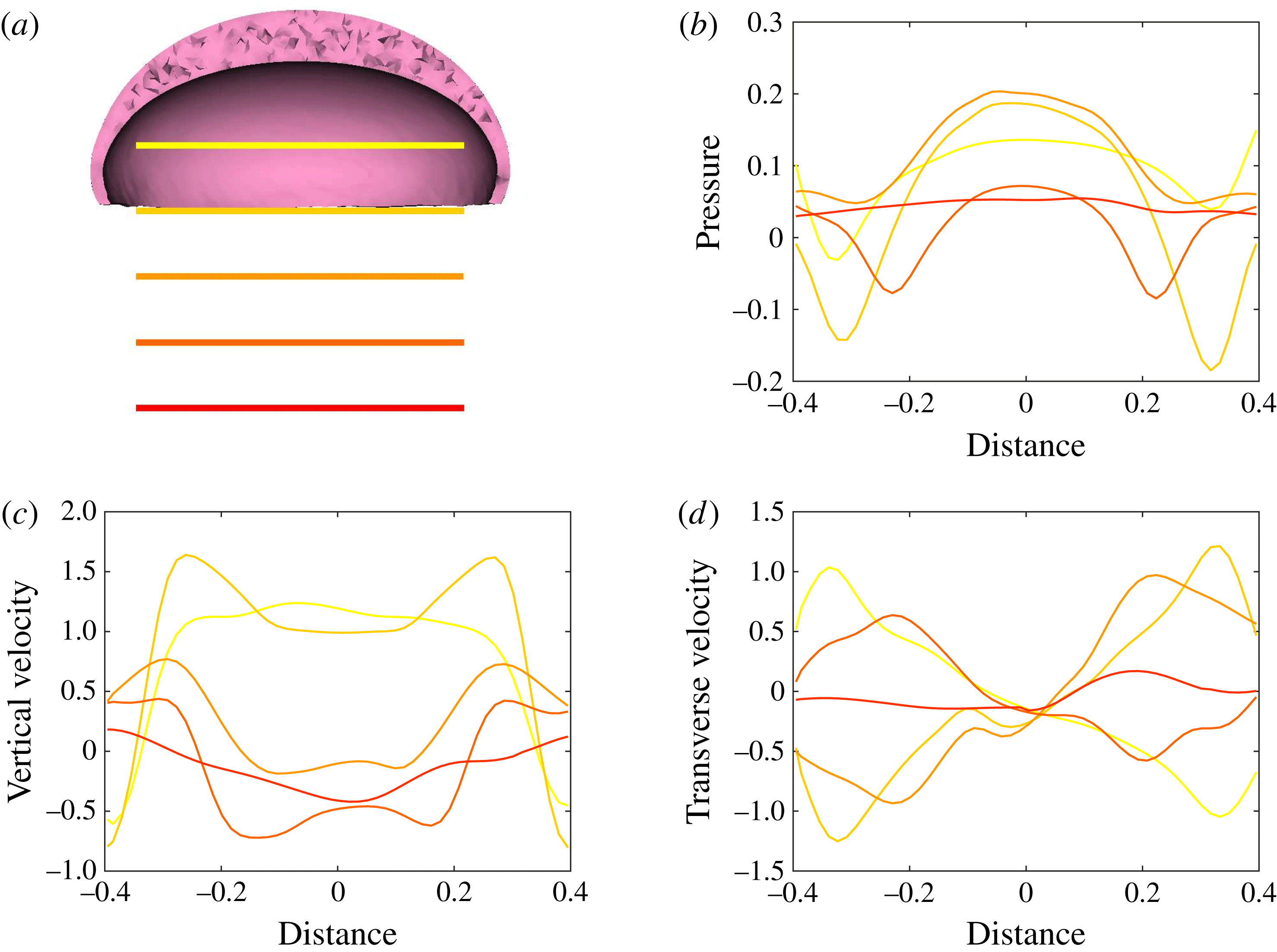
Plots corresponding to (a) the horizontal line out recordings of the Cartesian data (fluid velocity and pressure) at different vertical heights in the bell cavity and its wake at the end of the eighth propulsive cycle. Plotted are (b) the non-dimensional pressure (
 $\hat{p}$
), (c) non-dimensional vertical velocity (
 $\hat{u} _{z}$
) and (d) non-dimensional transverse velocity (
 $\hat{u} _{x}$
) with respect to the distance from the vertical axis. Recall that dimensionless velocities are given as bell heights travelled per half-propulsive cycle.
Snapshots of the bell during the propulsive cycle of the bell at times (a) 0, (b) 0.25, (c) 0.5, (d) 0.75, (e) 1.0, (f) 1.25, (g) 1.5, (h) 1.75 and (i) 2.0. Note that time is given in half-propulsive cycles. Bell colour indicates the instantaneous strength of contraction. During the contraction phase (b–e), active tension is applied to the margin of the bell. The bell is then allowed to expand (f–i) passively to its resting state. Note the buckling of the margin (f) when the tension is released.

Figure 10 shows the velocity vector field and a colour map of the vertical component of the dimensionless velocity (
 $\hat{u} _{z}$
) in and around the bell cavity during the eighth propulsive cycle. At the start of the eighth cycle (figure 10
a), there is a strong positive (upward) vertical flow within and immediately below the bell. Negative (downward) vertical velocity is seen within the stopping vortex ring, as found in figure 5. Though the bell is fully expanded at this point, the rotation of the stopping vortex ring generates a positive vertical velocity across the immediate wake. As the bell contracts (figure 10
b,c), a strong downward jet is generated as the fluid is pushed out of the subumbrellar cavity. Following contraction (figure 10
d), negative vertical velocity is found within the starting vortex ring which then joins the wake formed by the previous cycles’ starting vortex rings. After the expansion phase of the bell (figure 10
e), the interaction between the starting and stopping vortex rings directs the motion of the surrounding fluid towards the bell cavity, resulting in strong positive vertical flow.
The Cartesian grid data for pressure (
 $p$
), the vertical velocity (
 $u_{z}$
) and the transverse velocity (
 $u_{x}$
) along five different horizontal slices from within the bell cavity to the wake at the end of the eighth propulsive cycle were compared. In figure 11 we plotted the non-dimensional pressure (
 $\hat{p}$
), non-dimensional vertical velocity (
 $\hat{u} _{z}$
) and non-dimensional transverse velocity,
 $$\begin{eqnarray}\hat{u} _{x}=\frac{u_{x}}{\unicode[STIX]{x1D719}L_{h}},\end{eqnarray}$$
with respect to the horizontal axis
 $$\begin{eqnarray}\hat{x}=\frac{x}{L}.\end{eqnarray}$$
We found the presence of elevated positive pressure in the centre of the bell cavity in contrast with the low pressure points at the sides. Comparing these readings with figures 5–10, we note the location of the pressure minimums are found within the vortex rings. Comparing the vertical velocity readings at the different vertical coordinates, we found a strong positive flows in the centre of the subumbrellar cavity and downward flow along the subumbrellar surface. The direction of flow along the radial axis flips in the wake. Strong negative (downward) flow is observed along the central axis downstream of the jellyfish. Transverse velocity readings showed a minimum near the centre axis, with the sides alternating between positive and negative readings.
Snapshots of the spatial activation and release patterns of the bell can be seen for the reference configuration in figure 12. The bell contracts following the activation of tension along the bell margin (figure 12
a–e). The bell then expands as the applied tension is removed (figure 12
f–i). As the bell expands, its margin buckles. This effect is dependent on the material properties of the bell,
 $\unicode[STIX]{x1D702}_{m}$
and
 $\unicode[STIX]{x1D702}_{var}$
, which are examined subsequently. Buckling is not observed during the contraction of the bell, where the stress of the active tension dominates the passive elastic stresses of the deformed body. If the mesoglea were a homogenous incompressible material, then compression due to axial strains on the material would lead to an expansion in the transverse axial directions. The contributions of the bulk modulus, which are absent in our model, in turn could lead to buckling during the contraction phase. It is important to note that the mesoglea is a heterogeneous material due to the presence of radial fibres (Megill et al.
Reference Megill, Gosline and Blake2005) and additional work is needed to characterize the bulk modulus of this biological material (Wainwright Reference Wainwright1982) to fully examine mathematically whether or not the bell deforms in this way.
3.2 Varying the active and passive material properties of the bell
In the following set of simulations, the relationship between the passive and active material properties of the bell model are explored by varying the non-dimensional margin rigidity,
 $\unicode[STIX]{x1D702}_{m}$
, and the non-dimensional maximum applied tension,
 $T_{max}$
(see (2.11), (2.19) and (2.20)). In the first set of simulations, the passive elastic properties are held fixed and the active properties (e.g. the applied tension) are varied. In the second set of simulations, we hold the active properties fixed and vary the passive elastic properties of the margin. In the final set of simulations, both active and passive properties are varied so that the margin rigidity and maximum applied tension change in proportion. We then compare the cost of transport and
 $St^{-1}$
across this mechanospace. Movies for the following set of simulations can be found in the supplementary materials.
3.2.1 Varying applied tension
A comparison of bell displacement and swimming performance for varying magnitudes of dimensionless applied tension. Plotted are (a) the displacement of the bell (in bell heights),
 $\hat{X}_{z}$
, as a function of time (in half-propulsive cycles),
 $\hat{t}$
, (b) the spatially averaged radius of the margin (in bell diameters),
 $\hat{R}$
, during the seventh and eighth propulsive cycles as a function of time, (c) the forward swimming speed of the bell (in bell heights travelled per half-propulsive cycle),
 $\hat{U} _{z}$
, during the seventh and eighth propulsive cycles as a function of time, (d) the temporally averaged speed (in bell heights travelled per half-propulsive cycle) as a function of the cycle number and (e) the non-dimensional power,
 $\hat{P}_{m}$
, associated with the applied active tension driving the contraction of the bell. As tension was increased, the forward swimming speed and radial displacements also increased. Note that the oscillations in forward swimming speed during the expansion phase were similar for varying levels of tension even if the resulting swim speeds are different.

Plots of the out-of-plane vorticity,
 $\hat{\unicode[STIX]{x1D714}}_{y}$
, at the end of the eighth propulsive cycle with
 $T_{max}$
equal to (a) 16 000, (b) 32 000, (c) 48 000, (d) 64 000 and (e) 80 000. As tension is increased, the starting vortex rings become more defined and are advected farther from the bell (d,e). In the low tension case (a), no well-defined vortex rings are present in the wake of the bell.

Isocontour plots of the non-dimensional vertical velocity,
 $\hat{u} _{z}$
, at the end of the eighth propulsive cycle with
 $T_{max}$
equal to (a) 16 000, (b) 32 000, (c) 48 000, (d) 64 000 and (e) 80 000. As tension is increased, the volume of the region with positive vertical velocity increases in the wake of the bell. At
 $T_{max}=16\,000$
a small column of negative vertical velocity is present but there is no significant positive vertical velocity.

Isocontour plots of the non-dimensional radial component of velocity,
 $\hat{u} _{rad}$
, at the end of the eighth propulsive cycle with
 $T_{max}$
equal to (a) 16 000, (b) 32 000, (c) 48 000, (d) 64 000 and (e) 80 000. As tension is increased, the isocontour volume of the negative radial velocity increases in the immediate wake of the bell.

Isocontour plots of non-dimensional vorticity magnitude,
 $\hat{\unicode[STIX]{x1D714}}_{mag}$
, at the end of the first propulsive cycle with
 $T_{max}$
equal to (a) 16 000, (b) 32 000, (c) 48 000, (d) 64 000 and (e) 80 000. Note that for
 $T_{max}=80\,000$
, the starting vortex ring is advected farther from the bell than for
 $T_{max}=32\,000$
, 48 000 and 64 000. Note that
 $T_{max}=16\,000$
lacks a defined starting vortex ring.

(a) The COT, normalized by the cost of transport for the reference case (
 $COT_{ref}$
), and (b) the inverse Strouhal number,
 $St^{-1}$
, as a function of the magnitude of applied tension. Note that the cost of transport initially decreases as the magnitude of applied tension increases. For
 $T_{max}\geqslant 48\,000$
, we note that the cost of transport begins to increase slightly, suggesting an increased role of drag as the bell undergoes larger deformations.
 $St^{-1}$
increases as
 $T_{max}$
increases. Note that when
 $T_{max}\geqslant 48\,000$
, the bell is in the peak propulsive efficiency range,
 $0.2<St<0.4$
.

In this set of simulations, the bell’s passive elastic properties are held fixed at their reference values while the maximum applied tension is varied as
 $T_{max}=16\,000$
, 32 000, 48 000, 64 000, 80 000. The goal is to quantify how variations in the tension applied result in changes in the amount of bell contraction and the resulting swimming speeds. As the maximum applied tension is increased, the distance travelled by the bell,
 $\hat{X}_{z}$
, (figure 13
a) and the maximum radial displacement,
 $\hat{R}$
, (figure 13
b) increase. Figure 13(c) shows the forward swimming speeds as functions of time. We remark that the oscillations in forward swimming speed that occur during the passive expansion of the bell maintain a similar profile. The forward swimming velocity,
 $U_{z}$
, which is recorded at the top of the bell, reflects these oscillations following the rapid rise and decline induced by the activation and release of tension, respectively. High frequency oscillations are seen for larger values of applied tension from the larger deformations of the top of the bell. As
 $T_{max}$
increases, so does the steady-state swimming speed averaged over a propulsive cycle, as seen in figure 13(d). As
 $T_{max}$
increases, the peak power observed during the contraction phase also increases (figure 13
e).
Figure 14 shows the out-of-plane vorticity,
 $\hat{\unicode[STIX]{x1D714}}_{y}$
, at the end of the simulation for the different tension magnitudes. For
 $T_{max}\geqslant 48\,000$
, we note the presence of well-defined starting vortex rings present in the wake, along with a strong stopping vortex present in the bell cavity. In the case of
 $T_{max}=16\,000$
, we find a less well-defined vortex wake, which corresponds to negligible forward swimming speeds.
Comparing the isocontours of the non-dimensional vertical velocity,
 $\hat{u} _{z}$
, in figure 15, we find that increasing the magnitude of applied active tension increases the positive vertical velocity present in the immediate wake of the bell. Increasing the applied active tension yields a larger volume of negative radial velocity in the wake of the bell, as seen in figure 16.
Figure 17 shows contour plots of the non-dimensional vorticity magnitude,
 $\hat{\unicode[STIX]{x1D714}}_{mag}$
, after one propulsive cycle for each of the applied tensions. As the maximum applied tension increases, the distance between the starting vortex ring and the bell increases. For
 $T_{max}=16\,000$
, we note the absence of a starting vortex, whereas the plot of
 $T_{max}=80\,000$
shows a starting vortex present near the inner cavity of the bell.
The cost of transport and
 $St^{-1}$
for the different tension magnitudes are reported in figure 18(a,b), respectively. The cost of transport decreases as the maximum applied tension increases before plateauing at
 $T_{max}=48\,000$
and increasing slightly at
 $T_{max}=80\,000$
. This suggests that increased drag from faster steady swimming speeds play a role in increasing the cost of transport, since drag is proportional to velocity squared. Examining
 $St^{-1}$
, we found that increasing
 $T_{max}$
leads to higher
 $St^{-1}$
. Note that for
 $T_{max}\geqslant 48\,000$
, the swimming bell is within the peak propulsive efficiency range described by Taylor et al. (Reference Taylor, Nudds and Thomas2003).
3.2.2 Varying margin rigidity
A comparison of bell displacement and different metrics of swimming performance for varying elastic moduli of the bell margin with a fixed magnitude of applied tension. Plotted are (a) the displacement of the bell (in bell heights),
 $\hat{X}_{z}$
, as a function of time (in half-propulsive cycles),
 $\hat{t}$
, (b) the spatially averaged radius of the margin (in bell diameters),
 $\hat{R}$
, during the seventh and eighth propulsive cycles as a function of time, (c) the forward swimming speed of the bell (as bell heights travelled per half-propulsive cycle),
 $\hat{U} _{z}$
, during the seventh and eighth propulsive cycles as a function of time, (d) the temporally averaged speed (as bell height travelled per half-propulsive cycle) as a function of the cycle number and (e) the non-dimensional power,
 $\hat{P}_{m}$
, associated with the applied active tension driving the contraction of the bell. As the stiffness of the bell margin,
 $\unicode[STIX]{x1D702}_{m}$
, decreases, the forward swimming speed increases and the maximum radial displacement increases.

Plots of the non-dimensional out-of-plane vorticity,
 $\hat{\unicode[STIX]{x1D714}}_{y}$
, after the eighth propulsive cycle with
 $\unicode[STIX]{x1D702}_{m}$
equal to (a) 125, (b) 250, (c) 375, (d) 500 and (e) 625. As margin flexibility is increased, the starting vortex rings shed during the contraction become more defined and are advected farther downstream. For
 $\unicode[STIX]{x1D702}_{m}=625$
, no clear stopping vortex ring is present in the bell cavity.

Isocontour plots of the non-dimensional vertical velocity,
 $\hat{u} _{z}$
, at the end of the eighth propulsive cycle with
 $\unicode[STIX]{x1D702}_{m}$
equal to (a) 125, (b) 250, (c) 375, (d) 500 and (e) 625. As margin flexibility increases, the volume of fluid moving with substantial positive vertical velocity increases in the immediate wake of the bell. The strength and volume of fluid moving in the wake with negative vertical velocity also increases.

Isocontour plots of the non-dimensional radial velocity,
 $\hat{u} _{rad}$
, at the end of the eighth propulsive cycle with
 $\unicode[STIX]{x1D702}_{m}$
equal to (a) 125, (b) 250, (c) 375, (d) 500 and (e) 625. As margin flexibility increases, the volume of fluid moving with significant negative radial velocity increases in the immediate wake of the bell.

Isocontour plots of non-dimensional vorticity magnitude,
 $\hat{\unicode[STIX]{x1D714}}_{mag}$
, at the end of the first propulsive cycle with
 $\unicode[STIX]{x1D702}_{m}$
equal to (a) 125, (b) 250, (c) 375, (d) 500 and (e) 625. Note that for
 $\unicode[STIX]{x1D702}_{m}=125$
, the starting vortex ring is advected farther downstream after one propulsive cycle than for
 $\unicode[STIX]{x1D702}_{m}=250$
, 375, 500, 625.

(a) The COT normalized by the cost of transport of the reference configuration (
 $COT_{ref}$
), and (b) the inverse Strouhal number,
 $St^{-1}$
, as a function of elastic moduli of the bell margin with a fixed magnitude of applied tension. Note that the cost of transport dramatically increases as
 $\unicode[STIX]{x1D702}_{m}$
increases. As
 $\unicode[STIX]{x1D702}_{m}$
increases,
 $St^{-1}$
decreases. The bell is pumping in the optimal
 $St$
range when
 $\unicode[STIX]{x1D702}_{m}\leqslant 375$
.

A complementary study to § 3.2.1 is performed by holding the maximum applied tension fixed at
 $T_{max}=48\,000$
, and varying the margin rigidity,
 $\unicode[STIX]{x1D702}_{m}=125$
, 250, 375, 500, 625. The stiffness of the top of the bell,
 $\unicode[STIX]{x1D702}_{tot}$
, is held fixed by adjusting
 $\unicode[STIX]{x1D702}_{var}$
to account for variations in
 $\unicode[STIX]{x1D702}_{m}$
. As
 $\unicode[STIX]{x1D702}_{m}$
decreases, the distance travelled increases, figure 19(a), as does the time it takes the bell to expand, figure 19(b). Higher forward swimming speeds and higher average swimming speeds are noted in figure 19(c,d) for the cases of the more flexible bell margins. Figure 19(e) shows that the maximum power observed during the propulsive cycle decreases as
 $\unicode[STIX]{x1D702}_{m}$
increases, from the increased resistance from the passive elastic properties of the bell.
Figure 20 show the out-of-plane vorticity at the end of the simulation for different margin elasticities. As the elastic modulus of the margin decreases, more defined starting vortex rings appear in the wake of the bell, along with more defined complementary stopping vortex rings in the bell cavity. This is due to the fact that the bell is deforming more at lower stiffnesses. For the stiffest case,
 $\unicode[STIX]{x1D702}_{m}=625$
, the bell motion does not produce strong stopping vortex rings in the wake, corresponding with the slowest forward swimming speed.
Comparing the isocontours of the non-dimensional vertical velocity,
 $\hat{u} _{z}$
, in figure 21, we find that increasing margin flexibility also increases the positive vertical velocity present in the immediate wake of the bell. Increasing margin flexibility yields a larger volume of negative radial velocity in the wake of the bell, as seen in figure 22.
Examining the vorticity magnitude after the first propulsive cycle (figure 23), we note that as the elastic modulus of the margin decreases, the distance of the starting vortex ring from the bell increases as the jellyfish swims faster. A weak starting vortex does occur at lower tensions, but it is below the threshold for drawing the vorticity contours. In general, the swimming speed increases with the strength of the starting vortex.
The cost of transport and
 $St^{-1}$
for the different margin elastic moduli are examined in figure 24(a,b), respectively. As the margin elastic modulus is increased, the cost of transport increases as well. A dramatic increase is observed at
 $\unicode[STIX]{x1D702}_{m}=625$
.
 $St^{-1}$
decreases as the margin rigidity increases. At lower margin rigidities,
 $\unicode[STIX]{x1D702}_{m}\leqslant 375$
, the bell operates in the optimal
 $St$
range.
3.2.3 Varying the effective margin stiffness
A comparison of bell displacement and swimming performance when the magnitude of applied tension is held proportional to the non-dimensionalized elastic modulus. Plotted are (a) the displacement of the bell (in bell heights travelled),
 $\hat{X}_{z}$
, as a function of time (in half-propulsive cycles),
 $\hat{t}$
, (b) the spatially averaged radius of the margin (in bell diameters),
 $\hat{R}$
, during the seventh and eighth propulsive cycles as a function of time, (c) the forward swimming speed of the bell (as bell height travelled per half-propulsive cycle),
 $\hat{U} _{z}$
, during the seventh and eighth propulsive cycles as a function of time, (d) the temporally averaged speed (as bell height travelled per half-propulsive cycle) as a function of the cycle number and (e) the non-dimensional power,
 $\hat{P}_{m}$
, associated with the applied active tension driving the contraction of the bell. As margin stiffness was increased, the ratio between the magnitude applied tension and the elastic modulus was maintained. For
 $\unicode[STIX]{x1D702}_{m}=250$
, 375, 500, 625, the forward swimming speeds are similar to one another, even though there were some differences in radial displacement. The exception was
 $\unicode[STIX]{x1D702}_{m}=125$
, where the radial displacement and forward swimming speed were much less than the other cases.

The bell during the expansion phase (time
 $=$
1.25) for
 $\unicode[STIX]{x1D702}_{m}$
equal to (a) 125, (b) 250, (c) 375, (d) 500 and (e) 625.
 $T_{max}$
was varied in proportion to the elastic modulus. The spatial activation of tension is mapped onto the bell. Note that buckling modes present as
 $\unicode[STIX]{x1D702}_{m}$
is varied.

Snapshots of the bell margin deformation during the expansion phase of the first propulsive cycle for
 $\unicode[STIX]{x1D702}_{m}$
equal to (a) 125, (b) 250, (c) 375, (d) 500 and (e) 625. A movie comparing the movement of the bell margin for the total length of the simulation has been provided in the supplementary materials. Note that peak applied tension occurs near a time equal to 0.75, though the margin may continue to contract if the fluid forces from the surrounding environment are greater than the passive elastic forces. As
 $\unicode[STIX]{x1D702}_{m}$
decreases, we note the appearance of higher buckling modes at the bell margin. The timing of peak buckling amplitudes is also dependent on
 $\unicode[STIX]{x1D702}_{m}$
. As
 $\unicode[STIX]{x1D702}_{m}$
increases, the time it takes for the bell to fully expand decreases.

(a) The COT normalized by the cost of transport of the reference case (
 $COT_{ref}$
) and (b) the inverse Strouhal number,
 $St^{-1}$
, as a function of the elastic modulus of the margin with a proportional magnitude of applied tension. Note that the cost of transport increases as the margin elastic modulus and applied tension increase. Though
 $\unicode[STIX]{x1D702}_{m}=125$
has the lowest cost of transport, it is not in the range of
 $St$
characterized as giving peak propulsive performance. Here
 $\unicode[STIX]{x1D702}_{m}=250$
, 375 are in this optimal
 $St$
range before decreasing in performance as
 $\unicode[STIX]{x1D702}_{m}$
increases.

In §§ 3.2.1 and 3.2.2, we varied the maximum applied tension and the margin elasticity, respectively, to explore their role in swimming performance. In this section, the maximum applied tension is varied in proportion to the margin elastic modulus,
 $\unicode[STIX]{x1D702}_{m}\propto T_{max}$
. Using the ratio of the parameters of
 $T_{max}$
and
 $\unicode[STIX]{x1D702}_{m}$
from our reference case,
 $\unicode[STIX]{x1D702}_{m}$
is varied and
 $T_{max}$
is in turn adjusted to maintain the same proportionality. The vertical displacement of the bell (figure 25
a) and the average forward swimming speeds (figure 25
d) are examined, and we find that for
 $\unicode[STIX]{x1D702}_{m}\geqslant 250$
, the bells move at comparable forward swimming speeds. For
 $\unicode[STIX]{x1D702}_{m}=125$
, the bell is significantly slower than the other bells. Note that whereas the average speeds travelled during the propulsive cycle are similar for
 $\unicode[STIX]{x1D702}_{m}\geqslant 250$
, the forward swimming profiles (figure 25
c) following contraction and expansion of the bell vary significantly. Examining the radial displacement of the bell in figure 25(b), one notes the low radial displacement for
 $\unicode[STIX]{x1D702}_{m}=125$
and the more gradual passive expansion following the release of tension relative to the other cases. This result suggests that the force required to push the fluid out of the bell outweighs the force required to deform the elastic bell. Figure 25(e) shows that as
 $\unicode[STIX]{x1D702}_{m}$
increases, the magnitude of the maximum and minimum power during the propulsive cycle increases substantially.
Figure 26 shows the deformation of the bell and the activation pattern of the applied tension during the expansion phase at
 $t=1.25$
for the different values of
 $\unicode[STIX]{x1D702}_{m}$
. Snapshots of the tip of the bell margin during the expansion cycle for different
 $\unicode[STIX]{x1D702}_{m}$
are shown in figure 27. A movie comparing the movement of the bell margin for the total length of the simulation has been provided in the supplementary materials. The buckling patterns of the bell margin observed during the expansion of the bell result from the interaction between the elastic restorative force of the bell, any remaining active tension, and the force applied by the surrounding fluid. As
 $\unicode[STIX]{x1D702}_{m}$
decreases, we note the presence of high frequency buckling modes at the bell margin. We also note that maximum buckling deformations occur later in the expansion phase. Finally, the amplitude of the buckling pattern increases as
 $\unicode[STIX]{x1D702}_{m}$
increases.
Examining the cost of transport for the different choices of
 $\unicode[STIX]{x1D702}_{var}$
and
 $T_{max}$
(figure 28
a), we note that as both the bell margin elastic modulus and maximum applied tension increase, the cost of transport increases as well. This follows from the idea that more energy is required to deform the bell as
 $\unicode[STIX]{x1D702}_{m}$
increases, even though the resulting speeds remain relatively similar for values of
 $\unicode[STIX]{x1D702}_{m}\geqslant 125$
. Examining
 $St^{-1}$
for the different parameters in figure 28(b), we find that
 $\unicode[STIX]{x1D702}_{m}=250\,375$
have the peak performance. Since there are many metrics of efficiency and performance that have been used to describe animal locomotion, our use of two of the more common choices shows how the ‘best’ design may vary depending upon the metric used. While
 $\unicode[STIX]{x1D702}_{m}=125$
may have the lowest cost of transport, it is not swimming within the
 $St^{-1}$
range characterized as yielding optimal propulsive efficiency. On the other hand,
 $\unicode[STIX]{x1D702}_{m}=250\,375$
have a relatively low cost of transport and are in the optimal
 $St^{-1}$
range.
3.3 Varying the Reynolds number
A comparison of bell displacement and swimming performance as
 $Re$
is varied. Plotted are (a) the displacement of the bell (in bell heights),
 $\hat{X}_{z}$
, as a function of time (in half-propulsive cycles),
 $\hat{t}$
, (b) the spatially averaged radius of the margin (in bell diameters),
 $\hat{R}$
, during the seventh and eighth propulsive cycles as a function of time, (c) the forward swimming speed of the bell (in bell heights travelled per half-propulsive cycle),
 $\hat{U} _{z}$
, during the seventh and eighth propulsive cycles as a function of time, (d) the temporally averaged speed (in bell heights travelled per half-propulsive cycle) as a function of the cycle number and (e) the non-dimensional power,
 $\hat{P}_{m}$
, associated with the applied active tension driving the contraction of the bell. Note that decreasing
 $Re$
resulted in lower forward swimming speeds and reduced contractions of the bell.

Plots of the non-dimensional out-of-plane vorticity,
 $\hat{\unicode[STIX]{x1D714}}_{y}$
, for
 $Re=25$
at times (a) 0, (b) 1.0, (c) 2.0, (d) 3.0, (e) 4.0, (f) 5.0, (g) 6.0, (h) 10.0 and (i) 16.0. Recall that time is given in half-propulsive cycles so that eight pulses are shown. Note that while significant vorticity is generated during the contraction of the bell, the increased effective viscosity of the fluid leads to rapid dissipation of the starting vortices.

Plots of the non-dimensional out-of-plane vorticity,
 $\hat{\unicode[STIX]{x1D714}}_{y}$
, for
 $Re=2.5$
at times (a) 0, (b) 1.0, (c) 2.0, (d) 3.0, (e) 4.0, (f) 5.0, (g) 6.0, (h) 10.0 and (i) 16.0. Eight pulses are shown. As viscous forces nearly balance inertial forces, the flows generated are nearly reversible and no significant forward swimming is seen.

Plots of the non-dimensional out-of-plane vorticity,
 $\hat{\unicode[STIX]{x1D714}}_{y}$
, for
 $Re=2500$
at times (a) 0, (b) 1.0, (c) 2.0, (d) 3.0, (e) 4.0, (f) 5.0, (g) 6.0, (h) 10.0 and (i) 16.0. Decreasing the effective fluid viscosity results in a larger contribution of the margin buckling to the vortex wake.

Plots of the non-dimensional vertical velocity,
 $\hat{u} _{z}$
, at the end of the eighth propulsive cycle with for
 $Re$
equal to (a) 2.5, (b) 25, (c) 250 and (d) 2500. At
 $Re=2.5$
we note the loss of central column of negative vertical velocity in the wake of the bell, as had been seen in previous simulations. Decreasing the effective fluid viscosity, for
 $Re\geqslant 25$
, yields a larger of column of negative vertical velocity in the wake increases and a region of positive vertical velocity near the bell cavity.

(a) The COT normalized by the cost of transport for the reference case (
 $COT_{ref}$
), and (b) the inverse Strouhal number,
 $St^{-1}$
, as function of Reynolds number,
 $Re$
. As
 $Re$
decreases, the cost of transport increases dramatically. At
 $Re\geqslant 250$
, the bell is swimming in the peak propulsive
 $St$
range.

The swimming performance of the model is also dependent on the Reynolds number regime in which it swims. In this set of simulations, we examine the swimming performance at
 $Re=0.5$
, 2.5, 5, 25, 50, 250, 500, 2500. Reynolds number is adjusted by only modifying the dynamic viscosity,
 $\unicode[STIX]{x1D707}$
, of the fluid. Note that in the previous studies, the model bell swims at
 $Re=250$
. The material parameters of the bell are set to the reference configuration. We find that as
 $Re$
decreases, the distance travelled by the bell decreases dramatically (figure 29
a) and the cases where
 $Re\leqslant 5$
do not generate any significant net forward movement. We also find that decreasing
 $Re$
results in a significant reduction in the radial displacement of the bell margin, figure 29(b). Model bells swimming at higher
 $Re$
exhibit nearly identical radial displacements, while the forward swimming speed (figure 29
c) increases as
 $Re$
increases. Examining the average speed per propulsive cycle (figure 29
d) we find that substantial average swimming speeds are only generated for
 $Re\geqslant 25$
. Figure 29(e) shows that the maximum power decreases as
 $Re$
decreases.
The strength and advection of the vortices generated during the propulsive cycle are also affected by
 $Re$
. Examining the out-of-plane vorticity for
 $Re=25$
(figure 30), we find that the wake of the bell lacks the presence of well-defined starting vortex rings. Though significant vorticity is generated during the contraction of the bell, the increased amount of fluid damping leads to rapid dissipation of the starting vortices. Forward movement is generated almost entirely during the contraction phase of the propulsive cycle. Examining the vorticity generated for
 $Re=2.5$
(figure 31), we find that the viscous forces nearly balance the inertial forces generated during the propulsive cycles, and vortices dissipate before they separate from the bell. The flows generated are nearly reversible, and no significant forward swimming is seen. As the
 $Re$
increases to 2500, the vorticity generated during the propulsive cycle (figure 32) is similar to the reference case, with the presence of separated starting vortex ring in the wake and a stopping vortex ring in the bell following the expansion phase. The decrease in fluid damping results in stronger buckling of the margin.
Figure 33 shows isocontours of the non-dimensional vertical velocity,
 $\hat{u} _{z}$
. Significant differences are seen in the wake as
 $Re$
increases. At
 $Re=2.5$
, the nearly reversible flows generated during the propulsive cycle lead to regions of positive vertical velocity in the wake of the bell during the expansion phases. As
 $Re$
increases, a strong column of negative vertical velocity is found in the wake of the bell, as seen with previous higher
 $Re$
simulations. When
 $Re=25$
, there is a smaller region of positive vertical velocity in the immediate wake of the bell.
Comparing the cost of transport for different
 $Re$
(figure 34
a) we find that the cost of transport increases as
 $Re$
decreases. This implies that as
 $Re$
decreases and the viscous forces begin to balance the inertial forces generated during the bell contraction, the bell’s swimming performance decreases. At intermediate
 $Re$
, secondary thrust is lost as the bell comes to rest between the end of the contraction and the beginning of the next contraction. At lower
 $Re$
, the bell moves backwards during the expansion. Examining
 $St^{-1}$
, we see that
 $St^{-1}$
increases with
 $Re$
(figure 34
b). When
 $Re\geqslant 250$
, the bell swims within the range of peak propulsive efficiency. Note that
 $St^{-1}$
levels off for the higher
 $Re$
because the relative change of viscous effects in the higher
 $Re$
cases is relatively small.
3.4 Circulation analysis
Plots of the temporal evolution of the circulation,
 $\hat{\unicode[STIX]{x1D6E4}}$
, of the starting (red) and stopping (blue) vortex rings during the eighth propulsive cycle of the reference case. The circulation of the starting vortex ring decreases in a fairly linear manner as it advects away from the bell. The stopping vortex initially experiences a decline in circulation, followed by a plateau where the circulation does not substantially decrease. The stopping vortex ring’s peak circulation is substantially higher than that of the starting vortex ring.

Plots of the non-dimensionalized circulation,
 $\hat{\unicode[STIX]{x1D6E4}}$
, of (a) the starting vortex ring, (b) the stopping vortex ring and (c) the total wake (i.e. the sum of the computed circulation of each starting vortex ring present in the wake) at the end of each propulsive cycle for differing
 $\unicode[STIX]{x1D702}_{m}$
of the varying effective margin stiffness study. We note that the circulation associated with the starting and stopping vortex rings does not change substantially when comparing from cycle to cycle. The circulation associated with the wake, which includes the circulation of every starting vortex ring from previous cycles, initially increases with each propulsive cycle before plateauing as contributions of the most recent propulsive cycle are balanced with the viscous dissipation of the previous cycles’ starting vortex rings.

Plots of the non-dimensionalized circulation,
 $\hat{\unicode[STIX]{x1D6E4}}$
, associated with the eight propulsive cycle’s starting vortex ring (red), stopping vortex ring (blue) and wake (green), for (a) the varying tension study, (b) the fixed tension study and (c) the Reynolds number study. The circulation increased as the maximum applied tension,
 $T_{max}$
increased and margin stiffness was held constant. The circulation increased as the margin stiffness (
 $\unicode[STIX]{x1D702}_{m}$
) decreased and
 $T_{m}$
was held constant. In the Reynolds number study, we found that the circulation increased as the Reynolds number increased.

To quantify how the fluid is affected by variations in the medusan mechanospace, an analysis of the circulation of the vortex rings was performed. Following the methods of Colin et al. (Reference Colin, Costello, Dabiri, Villanueva, Blottman, Gemmell and Priya2012), we calculated circulation,
 $\unicode[STIX]{x1D6E4}$
, as the integral of vorticity over the area of the vortex ring along the central plane as
 $$\begin{eqnarray}\unicode[STIX]{x1D6E4}=\int \unicode[STIX]{x1D714}_{y}(x,0,z,t)\,\text{d}x\,\text{d}z,\end{eqnarray}$$
which was then non-dimensionalized with respect to the characteristic length,
 $L$
, and driving frequency,
 $\unicode[STIX]{x1D719}$
,
 $$\begin{eqnarray}\hat{\unicode[STIX]{x1D6E4}}=\frac{\unicode[STIX]{x1D6E4}}{L^{2}\unicode[STIX]{x1D719}}.\end{eqnarray}$$
The temporal evolution of the non-dimensional circulation of the starting and stopping vortex rings during the final propulsive cycle was recorded (figure 35). Both the starting and stopping vortex rings exhibit the most circulation when they initially form. We found that the peak circulation of the stopping vortex was substantially greater that the peak circulation of the starting vortex, confirming the experimental observations of Gemmell et al. (Reference Gemmell, Costello, Colin, Stewart, Dabiri, Tafti and Priya2013). The starting vortex ring’s circulation decays in time in a linear manner, with a steady decline following the initial peak. The circulation of the stopping vortex initially declines. The circulation then plateaus such that the stopping vortex ceases to substantially decay in time. This points to the continued role of the stopping vortex in producing secondary thrust during the passive energy recapture phase of the propulsive cycle.
The evolution of the non-dimensional circulation over each cycle was recorded for different effective margin stiffnesses,
 $\unicode[STIX]{x1D702}_{m}$
, at the end of each propulsive cycle (figure 36). In figure 36(a,b), the evolution of the circulation of the starting and stopping vortex ring, respectively, are shown for each propulsive cycle. We note that the circulation for the starting and stopping vortex rings remains fairly stable from one propulsive cycle to another. We also note that in all cases the stopping vortex ring has a higher circulation at the end of the cycle than the starting vortex ring. In figure 36(c), the circulation associated with the wake of the bell was also recorded by summing the circulation of each of the vortex rings present in the wake of the bell from previous propulsive cycles, including the most recent propulsive cycle. This measure allows us to quantify the contribution of all of the vortex rings in maintaining of the column of negative vertical velocity that pulls fluid away from the bell, as described in Dabiri et al. (Reference Dabiri, Colin, Costello and Gharib2005). We find the circulation of the wake initially increases as more vortex rings are formed with each propulsive cycle, but that the recorded circulation plateaus later in the simulation as the rate of additional circulation from the most recent propulsive cycle is balanced by the loss of circulation in the vortex structures due the viscous dissipation.
Noting the relative stability of the recorded circulation when the bell has reached a steady state, the non-dimensional circulation of the vortex structures at the end of the eighth propulsive cycle for the other simulations in this study are plotted in figure 37. In figure 37(a), the circulation of the starting vortex ring, stopping vortex ring and wake for the simulations of the varying tension study (§ 3.2.1) are plotted with respect to the maximum applied tension,
 $T_{max}$
. We note that the circulation increases as
 $T_{max}$
increases. Figure 37(b) similarly shows the circulation of the vortex rings in the fixed tension study (§ 3.2.2) with respect to the margin’s elastic modulus,
 $\unicode[STIX]{x1D702}_{m}$
. We found that as
 $\unicode[STIX]{x1D702}_{m}$
decreases and
 $T_{max}$
is held constant, the circulation of the wake and the circulation of the starting vortex rings increase, while the stopping vortex ring circulation increases to a lesser degree. In the Reynolds number study, figure 37(c), increasing fluid damping, such as in the
 $Re=25$
case, reduces the circulation. Note that in this case the wake’s circulation is nearly identical to that of the starting vortex ring. Due to the high amount of viscous dissipation, the wake’s circulation has negligible contributions from the vortex rings of previous cycles. Circulation increases as Reynolds number increases.
4 Discussion
Plots of the velocity vector field and vorticity at the end of the propulsive cycle for (a) the oblate jellyfish model of Park et al. (Reference Park, Chang, Huang and Sung2014), (b) our model and (c) particle image velocimetry (PIV) recordings of an Aurelia spp. from Gemmell et al. (Reference Gemmell, Costello, Colin, Stewart, Dabiri, Tafti and Priya2013) (note that the vorticity legend colour is flipped). In the labels of (a),
 $1^{\ast }$
is the vorticity due to the shear layer of the inner wall,
 $2^{\ast }$
is the vorticity from recovery stroke of the previous expansion phases, and
 $4^{\ast }$
is the vorticity resulting from the recovery stroke of the most recent expansion phase. Our model finds good qualitative agreement in the flow field and vorticity with the PIV recording from Gemmell.

In the computational studies reported herein, we found: (i) our model jellyfish with fixed elastic properties swims faster when more tension is applied; (ii) for a fixed applied tension, more flexible bell margins result in faster swimming speeds and lower costs of transport; (iii) similar swimming speeds can be obtained when the stiffness of the bell margin and the applied tension (above some minimum threshold) are varied in proportion for sufficiently large stiffnesses; (iv) although similar swimming speeds are generated when tension and stiffness are varied proportionally, the cost of transport increases with stiffness; (v) different buckling patterns occur for different bell margin stiffnesses; (vi) the swimming performance of the oblate bell decreases dramatically for
 $Re$
below 250; and (vii) a circulation analysis of the starting and stopping vortex rings showed that their strengths were dependent on the relative strength of activation with respect to the bell margin flexibility. Overall, our results demonstrate that flexible margins with sufficient tension to generate large deformations result in fast swimming at a low cost of transport. This helps to explain how jellyfish with swimming muscles that are only one cell layer thick are able to swim effectively: very flexible bell margins that undergo large deformations under small applied tensions are still effectively stiff enough to re-expand before the next contraction.
Oblate jellyfish have a relatively low cost of transport when compared to other swimming animals (Gemmell et al.
Reference Gemmell, Costello, Colin, Stewart, Dabiri, Tafti and Priya2013). With a muscle mass that compromises
 ${<}1\,\%$
of their body mass (Costello, Colin & Dabiri Reference Costello, Colin and Dabiri2008), the slow but low energetic cost of paddling jellyfish swimming compares favourably to faster swimming in fish. It should be emphasized that this does not apply to jetting jellyfish, which have relatively high cost of transport on par with flying (Daniel Reference Daniel1985). While exploring the active and passive material properties of our model, we find that increasing the ratio of the strength of muscular output to margin flexibility does decrease the cost of transport (figures 24
a and 18
a). Holding this ratio fixed while varying margin stiffness shows that decreasing margin stiffness results in lower cost of transport as long as the stiffness is sufficiently high (figure 28
a). It is also important to note that drag plays an increased role in raising the cost of transport as the deformation of the bell increases.
Our results are consistent with the experimental results of Gemmell et al. (Reference Gemmell, Costello, Colin, Stewart, Dabiri, Tafti and Priya2013) who recorded the swimming speeds of different species of jellyfish. They note that significant distances are travelled during the passive phases of the jellyfish swimming cycle. The first passive phase, called the passive expansion phase, occurs after contraction when the bell re-expands as a result of stored elastic energy. The second passive phase, called the passive energy recapture phase, occurs at the end of the bell expansion and before the next contraction. Their results suggest that the variation in swimming speed during both passive phases can be explained by the differences in bell morphology and mechanics.
In figure 38, we compare the velocity vector field and vorticity at the end of a propulsive cycle for the reference case with that of the three-dimensional oblate jellyfish model presented by Park et al. (Reference Park, Chang, Huang and Sung2014). Also provided are the velocity vector field and vorticity recorded by Gemmell et al. (Reference Gemmell, Costello, Colin, Stewart, Dabiri, Tafti and Priya2013) of an Aurelia spp. after a full propulsive cycle. The Park model shows positive vertical velocities in the wake and cavity of the bell, with vorticity due to the recovery stroke of the expansion phase and shear contributions from the bell’s boundary layer. The model presented by Park closely matched the velocity profile recorded in McHenry & Jed (Reference McHenry and Jed2003). In our model, we observe the interaction between the starting and stopping vortex ring in the immediate wake of the bell, with positive vertical velocity in the immediate wake of the bell and negative vertical velocity farther down the wake. Our model finds good qualitative agreement with the flow and vorticity observed by Gemmell. The novelty of our study is due to the fact that the bell motion and forward swimming speed emerges entirely from the active and passive material properties of the bell and its interaction with the fluid.
By examining the vertical and radial velocities of the surrounding fluid environment, our simulations capture the interaction between the stopping and starting vortex rings first noted by Dabiri et al. (Reference Dabiri, Colin, Costello and Gharib2005). Figures 9–11 show how the opposing directionality of the starting and stopping vortices pull fluid away from the bell and towards the subumbrellar cavity, allowing for passive energy recapture to occur. The simulations also produce a high pressure region in the cavity and a low pressure region in the surrounding fluid (figures 11 b and 9 c), confirming observations by Gemmell et al. (Reference Gemmell, Colin, Costello and Dabiri2015a ) post-expansion. The experimental results of their study suggest a low pressure region upstream of the jellyfish allows the animals to effectively pull themselves through the fluid via a suction force generated by paddling.
In §§ 3.2.1 and 3.2.2, we find that increasing the ratio of the strength of muscular output to margin flexibility, either by increasing the magnitude of applied tension or increasing the margin flexibility, increases the distance between the starting and the stopping vortex rings (figures 17 and 23). Note that this distance also increases during each subsequent contraction as the jellyfish reaches its steady-state swimming speed. Examining this effect with respect to the vertical and radial component of velocity (figures 15, 16, 21 and 22), we find that increasing the distance between the starting and stopping vortex rings entrains more fluid from outside the bell towards the subumbrellar cavity, which enhances the secondary thrust gained during passive energy recapture. This effect depends on the relative strength of the muscular output with respect to the minimum force required to push fluid out of the subumbrellar cavity, as seen in §§ 3.2.3 and 3.3.
In this study, both the cost of transport and Strouhal number were used as performance metrics to examine the swimming performance of the bell. The cost of transport, which is a measure of the energy spent per unit distance travelled, is calculated as a function of the applied active tension, the speed of the bell’s radial displacement and resulting distance travelled. The Strouhal number is instead a function of the driving frequency, radial displacement and forward swimming speed. Inverting the Strouhal number yields a non-dimensionalization of the forward swimming speed with respect to the radial displacement of the bell. Both metrics have been used to examine swimming in the context of animal locomotion (Taylor et al. Reference Taylor, Nudds and Thomas2003; Gemmell et al. Reference Gemmell, Costello, Colin, Stewart, Dabiri, Tafti and Priya2013; Hoover & Miller Reference Hoover and Miller2015). Taylor et al. (Reference Taylor, Nudds and Thomas2003) found that optimal animal locomotion occurs at Strouhal numbers that range between 0.2 and 0.4. Gemmell et al. (Reference Gemmell, Costello, Colin, Stewart, Dabiri, Tafti and Priya2013) noted that jellyfish take advantage of the vortex ring interactions to lower their cost of transport. Generally, we note that increasing the relative strength of active tension resulted in observed Strouhal numbers that were within the optimal Strouhal number range described by Taylor (figures 18 b and 24 b). The cost of transport generally decreased as the relative strength of applied tension increased (figures 18 a and 24 a), though we note in § 3.2.1 that the cost of transport plateaued as the strength of applied tension increased. When varying the effective margin stiffness in § 3.2.3, the magnitude of the active tension relative to the margin flexibility was held fixed. As the applied tension was varied in proportion to the margin flexibility, we found that the cost of transport decreased as margin stiffness decreased (figure 28 a) and the observed Strouhal numbers were only in the optimal ranges for intermediate values of the margin elastic modulus (figure 28 b). For the bell with the lowest elastic modulus, we note that it had the lowest cost of transport. In addition, the resulting forward swimming speed was lower and therefore yielded a Strouhal number that is outside the optimal range described by Taylor. This observation highlights the differences between the two metrics and demonstrates how they can be used to characterize optimal swimming performance.
Our computational results show that the elastic properties of the bell have a notable effect on the forward swimming speed during the passive re-expansion. In all cases, the maximum stiffness at the top of the bell,
 $\unicode[STIX]{x1D702}_{tot}$
, was held constant, and the flexibility of the bell margin was varied by changing
 $\unicode[STIX]{x1D702}_{var}$
and
 $\unicode[STIX]{x1D702}_{m}$
. In all cases, the forward swimming velocity initially experiences a rapid rise due the contraction of the bell, followed by a rapid decrease in velocity once tension is released. During the passive energy recapture phase, the stopping vortex created during the expansion recaptures some of the momentum transferred from the bell to the fluid during the contraction phase. This recapture sustains the velocity of the bell after both the contraction and the expansion have ended (Gemmell et al.
Reference Gemmell, Costello, Colin, Stewart, Dabiri, Tafti and Priya2013). The dynamics of the passive response is dependent upon the bell deformation induced by the contraction as well as the spatial organization of the bell’s elastic properties. After the contraction phase, the bell freely relaxes back to its resting configuration. Since our model is an underdamped system, some elastic oscillations of the bell are observed and affect the observed shear layers of vorticity during the expansion phase.
Similar to experimental results, the elastic properties of the bell affect the gains from passive energy recapture, resulting in different average steady-state swimming velocities (figure 25 d). Gemmell et al. (Reference Gemmell, Costello, Colin, Stewart, Dabiri, Tafti and Priya2013) found that the 32 % of the total distance travelled occurs during this passive energy recapture phase. In the computational model, we find that during passive energy recapture phase the reference bell travelled 26 % of the total distance travelled (figure 39 a). In this case, the passive energy recapture phase represents 40 % of the total propulsive cycle. We find that keeping tension proportional to margin rigidity results in similar distances travelled (figure 39 b). In cases where the margin is more flexible and the magnitude of applied tension is held constant, the bell travels 30 % of the total distance of the propulsive cycle. Conversely, increasing rigidity while keeping tension fixed reduces the per cent of distance travelled during passive recapture to as low as 2 %.
Passive energy recapture comparison. (a) The velocity profile of the seventh propulsive cycle with regions demarcating the contraction phase (I), the expansion phase (II) and the passive energy recapture phase (III). The passive energy recapture phase represents 40 % of the total propulsive cycle. (b) The fraction of distance travelled during the passive expansion phase over the total distance travelled in the seventh propulsive cycle as a function of the elastic modulus of the margin. The two curves represent when the applied tension is held fixed (red, § 3.2.3) and when applied tension is held proportional to the margin stiffness (blue, § 3.2.2).

In the circulation analysis performed in § 3.13, the peak circulation of the stopping vortex ring was greater than that of the same propulsive cycle’s starting vortex ring, as had been observed in Gemmell et al. (Reference Gemmell, Costello, Colin, Stewart, Dabiri, Tafti and Priya2013). Furthermore, we found that while the starting vortex ring circulation declined linearly during the expansion phase of propulsive cycle, the stopping vortex ring circulation plateaus following an initial decline. The sustained circulation of the stopping vortex ring reveals its effectiveness in generating additional thrust during the passive energy recapture phase. The presence of this observation highlights the interplay of the roles passive energy recapture in lowering the cost of transport of forward swimming.
Little variability was observed in cycle-to-cycle changes in the circulation of the starting and stopping vortex rings (figure 36 a,b). The circulation of the wake of the bell initially increases with each additional starting vortex ring (figure 36 c). After several propulsive cycles, the circulation of the wake ceases the grow at which point the growth rate of circulation due to additional starting vortex rings is balanced by the decline in circulation due to viscous dissipation of previous cycles’ vortex rings. The limited cycle-to-cycle variation of the starting and stopping vortex rings suggest that steady-state swimming speeds emerge from the inertial contributions and viscous dissipation of the wake, as described in Dabiri et al. (Reference Dabiri, Colin, Costello and Gharib2005).
Examining the circulation of the eighth propulsive cycle of the varying tension study (figure 37 a) and fixed tension study (figure 37 b), we find that circulation increases as the relative magnitude of applied tension increases. When the magnitude of applied tension is low relative to the margin flexibility, the contributions of the starting vortex ring to circulation are lower. Furthermore viscous dissipation of the previous cycles’ vortex rings leads to negligible contributions of circulation from the far wake of the bell. As the Reynolds number is lowered (figure 37 c), we also note the decrease in circulation. At lower Reynolds numbers, the contributions to circulation are primarily only from the most recent pair of vortex rings. As the Reynolds number increases, the circulation due to the stopping vortex ring does not substantially change, but the contributions of wake and starting vortex rings increase as there is less viscous dissipation.
In this present study, only the margin rigidity and the strength of applied tension were varied. The frequency of free vibration of the bell was kept greater than the driving frequency,
 $\unicode[STIX]{x1D719}$
, so as to ensure that the bell fully expanded before the next contraction. We also only considered oblate bells, whereas Hoover and Miller showed resonant driving gains in prolate bells (Hoover & Miller Reference Hoover and Miller2015). Furthermore, active tension was only applied during the contraction stage, whereas other resonant studies (Demont & Gosline Reference Demont and Gosline1988b
; Hoover & Miller Reference Hoover and Miller2015) apply a sinusoidal force or prescribe sinusoidal bell deformations such that active force is applied during the entire swimming stroke. These differences make it difficult to describe the gains made by resonant driving relative to previous work. Furthermore, passive energy recapture’s role in lowering of the cost of transport should be examined with respect to resonant driving to determine the optimal driving frequency of the bell. Future studies should determine the frequency of free vibration of the different bell models and measure the resulting swimming speeds when driving over a large range of frequencies.
Although a comprehensive study on the role of buckling on swimming performance is outside the scope of this paper, we can still comment on the resulting margin buckling patterns that were observed in § 3.2.3. The buckling patterns found in figures 26 and 27 suggest that the variation in elastic response during the expansion will impact vortex deposition in the bell cavity, as suggested in previous studies (Colin et al. Reference Colin, Costello, Dabiri, Villanueva, Blottman, Gemmell and Priya2012; Gemmell et al. Reference Gemmell, Costello and Colin2014). Such changes in vortex deposition alter the effective Strouhal number. When the ratio of tension to margin rigidity was held fixed and the margin rigidity was varied (figure 28 b), we found that the optimal Strouhal range is reached for intermediate margin flexibilities. This suggests that there is an optimal flexibility when the strength of applied tension to margin flexibility ratio is held fixed. Higher buckling modes could have negative effects on the formation of stopping vortex rings in the bell. In turn, too flexible of a bell margin leads to an expansion phase that is too long, reducing the transfer of momentum from the bell to the fluid. Likewise, a bell margin that is not flexible enough may yield too short of an expansion phase and reduce the secondary thrust associated with passive energy recapture, resulting in a lower forward swimming speeds. Scalloping of the bell margin has also been observed (Colin et al. Reference Colin, Costello, Dabiri, Villanueva, Blottman, Gemmell and Priya2012) and may play role in reducing the buckling observed during the expansion. The presence of radial musculature in the bell margin could also play a role in the resulting kinematics of the bell margin and alter the buckling patterns during expansion (Megill et al. Reference Megill, Gosline and Blake2005; Gemmell et al. Reference Gemmell, Troolin, Costello, Colin and Satterlie2015b ). Previous studies suggest the presence of radial joints in the interior walls of the subumbrellar cavity (Gladfelter Reference Gladfelter1972; Megill et al. Reference Megill, Gosline and Blake2005) that allow for a robust mechanism for maintaining low amplitude, regular deformation kinematics during the contraction and expansion.
In conclusion, the development of this three-dimensional elastic model of jellyfish allows for future investigations on how manoeuvres are controlled through the asymmetric contraction of muscles, how the entire elastic bell (including the thick region of mesoglea at the top) may be tuned for resonant driving, whether or not the elastic properties of the bell are optimized for efficient swimming and how groups of jellyfish may enhance or impede feeding currents. Such numerical investigations are capable of addressing questions related to how the resulting kinematics measured by experimentalists emerge from the interaction of neurally activated muscles that drive elastic bells that are fully coupled to water. These answers may provide insight into the evolution of Cnidarian morphologies and may inform the design of biologically inspired, flexible underwater vehicles.
Acknowledgements
We would like to thank T. Hedrick and W. Kier for their advice and insights throughout this research project. This research was funded by a National Science Foundation (NSF) DMS CAREER no. 1151478 (to L.A.M.), an NSF DMS Research and Training Grant no. 5-54990-2311 (to R. McLaughlin, R. Camassa, L.A.M., G. Forest and P. Mucha), an NSF ACI Collaborative Research Grant no. 1450327 (to B.E.G. and R. O’Bara) and an NSF DMS Continuing Grant no. 1460368 (to B.E.G). We would also like to thank other members of the Mathematical Physiology Group at UNC, such as L. Waldrop, A. Baird, N. Battista, S. Jones, J. Samson, G. McLaughlin, and A. Porras. Images were created with VisIt and Matlab.
Supplementary materials
Supplementary materials are available at https://doi.org/10.1017/jfm.2017.3.



