INTRODUCTION
Our understanding of eolian systems of the past is usually either derived from modeled data or interpreted from ground data (e.g., the orientations and sedimentology of eolian landforms or spatial trends in eolian sediments such as loess or cover sand). The most commonly used small-scale model for such applications is the COHMAP (Cooperative Holocene Mapping Project) model (COHMAP Members, 1988), which depicts a glacial anticyclone near the southern margins of the Laurentide Ice Sheet (LIS) in summer (Hobbs, Reference Hobbs1943; Bryson and Wendland, Reference Bryson and Wendland1967). Data from large spits, eroded headlands on islands, and deltas in glacial Lake Algonquin, which spanned the southern margins of the ice sheet in the upper Great Lakes region between 13,300 and 11,500 cal yr BP, point to strong easterly winds within ≈150–200 km of the ice front (Krist and Schaetzl, Reference Krist and Schaetzl2001; Vader et al., Reference Vader, Zeman, Schaetzl, Anderson, Walquist, Freiberger, Emmendorfer and Wang2012; Schaetzl et al., Reference Schaetzl, Krist, Luehmann, Lewis and Michalek2016). Such winds, at a latitude normally dominated by westerly flow, support the concept of a glacial anticyclone, as do dune orientations in Saskatchewan, Canada (David, Reference David1981), and other on-ground data (for a review, see Schaetzl et al., Reference Schaetzl, Krist, Luehmann, Lewis and Michalek2016). Thus, ground data, if they derive from wind-influenced deposits or landforms at or near former ice marginal locations, can often be used to test the veracity of modeled data.
Nonetheless, the spits and islands of glacial Lake Algonquin are all immediately proximal to a part of the ice sheet with a generally east-to-west trending margin, where easterly winds would have been minimally disrupted by the geography of the ice margin. Other locations, where more lobate ice sheet margins existed, would undoubtedly have had much more complex wind patterns. Our study area is one such example. Another is in northeastern Wisconsin, where, based on textural and thickness patterns of loess, Schaetzl and Attig (Reference Schaetzl and Attig2013) reported evidence for easterly and westerly winds, presumably influenced by katabatic winds off the Lake Michigan and Ontonogan/Keweenaw Bay lobes. Small deposits of loess in Michigan’s Upper Peninsula also point to loess deposits formed on variable winds, perhaps resulting from the complex interaction of katabatic winds with the westerlies, coupled with a weakening glacial anticyclone (Kilibardia and Blockland, Reference Kilibarda and Blockland2011; Luehmann et al., Reference Luehmann, Schaetzl, Miller and Bigsby2013). Thus, additional ground data from other eolian features and deposits in the Great Lakes region could help refine our understanding of paleocirculation patterns and atmospheric drivers of eolian deposition in this region at the last glacial maximum (LGM) and continuing into the Holocene.
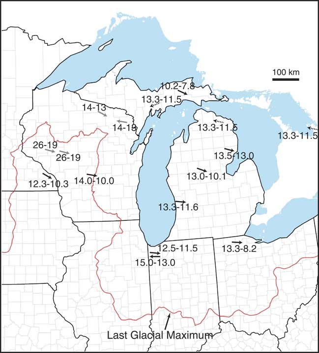
Slowly, data continue to accrue on the strength, directionality, and geographic extent of past eolian systems in the Great Lakes region. For example, research on sand dune orientations in the central Great Lakes region, for the period 14,000 to 10,000 yr BP, provides data for westerly winds at locations not near the ice margin during the latest Pleistocene. Dunes in central Lower Michigan—only about 200–250 km south of the ice margin—suggest that westerly and northwesterly winds were dominant here between 13,000 and 10,000 yr BP (Arbogast et al., 2015; Fig. 1). Dunes in central Wisconsin, slightly farther from the ice margin, were also formed by westerly winds between 14,000 and 10,000 yr BP (Rawling et al., Reference Rawling, Hanson, Young and Attig2008). In the Driftless Area of Minnesota near the Root River, eolian sands were deposited as sand ramps and on ridge crests on slopes facing north-northwest, indicating transport by northwesterly winds. Basal sands here were deposited between 12,300 and 10,300 yr BP (Hanson et al., Reference Hanson, Mason, Jacobs and Young2015). Elsewhere in Minnesota, predominantly northwesterly winds drove Holocene eolian systems (Grigal et al., Reference Grigal, Severson and Goltz1976; Keen and Shane, Reference Keen and Shane1990).
(color online) Locations of study sites in the upper Midwest that report on wind directions in the Late Pleistocene or early Holocene. Dune sites near the Great Lakes’ shoreline are not shown because they are influenced by not only regional winds but also local winds and sand supply, and because they cannot build out, into the lake, even if prevailing winds would force that to happen. Large-scale, Late Pleistocene transport of loess on generally westerly winds, out of north–south flowing meltwater river valleys, has long been known for this region and is therefore not shown here. Compiled from Arbogast et al. (2015, 2017), Campbell et al. (Reference Campbell, Fisher and Goble2011), Colgan et al. (Reference Colgan, Amidon and Thurkettle2017), Hanson et al. (Reference Hanson, Mason, Jacobs and Young2015), Kilibarda and Blockland (Reference Kilibarda and Blockland2011), Krist and Schaetzl (Reference Krist and Schaetzl2001), Loope et al. (Reference Loope, Fisher, Jol, Goble, Anderton and Blewett2004), Rawling et al. (Reference Rawling, Hanson, Young and Attig2008), Schaetzl et al. (Reference Schaetzl, Forman and Attig2014, Reference Schaetzl, Krist, Luehmann, Lewis and Michalek2016), Stanley and Schaetzl (Reference Stanley and Schaetzl2011), and Vader et al. (Reference Vader, Zeman, Schaetzl, Anderson, Walquist, Freiberger, Emmendorfer and Wang2012). Black arrows indicate data from dunes, gray arrows indicate data from loess, dashed arrows indicate data from spits or other features. Ages shown are best estimates based on ages cited in the original paper or the best estimates of the authors.

Despite our growing understanding of Quaternary eolian systems in this region, a considerable number of spatial and temporal gaps remain (Fig. 1). Ground data from underrepresented areas and for systems of different (or unknown) ages are key to refining any models or resolving any hypotheses about past eolian systems in this region. Such data are also needed to help interpret their spatiotemporal linkages to other geomorphic systems and to evaluate their paleoenvironmental significance. Our work is designed to address this gap by focusing on eolian systems and landforms in western and west-central Wisconsin, to help understand eolian systems here during the Late Pleistocene and into the Holocene, focusing on the lower Chippewa River valley (LCRV). Not only do deposits and landforms here suggest a strong west-northwesterly wind regime during the immediate postglacial period, but the widespread nature and longevity of eolian activity here points to a landscape that was unstable for considerable periods of time.
We argue that ground data on eolian sediments and landforms can assist paleoclimate models and help us to understand the postglacial climate of the region. Because the study area contains many bedrock ridges and inselbergs, we hypothesize that the pattern of eolian sediments and features near such “obstructions” may provide insight into paleowind directionality and strength. To that end, we will describe a variety of sandy and silty eolian deposits and landforms in the LCRV, to estimate the direction of winds responsible for their formation. Age data, limited though it may be at present, will help establish a preliminary chronology for some of these deposits.
STUDY AREA
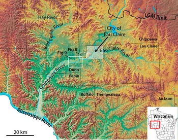
Much of our work is focused in or near the LCRV, immediately south on the terminal moraine of the LIS (Fig. 2; Faulkner et al., Reference Faulkner, Larson, Jol, Running, Loope and Goble2016). The Chippewa River is a major tributary to the upper Mississippi River in west-central Wisconsin. The upper Chippewa watershed was glaciated during Marine Oxygen Isotope Stage (MIS) 2 (i.e., the Late Wisconsinan glaciation). MIS 2 ice advanced into the Chippewa River basin from the north, as part of the Chippewa lobe, between ca. 18,500 and 22,000 yr ago (Schaetzl et al., Reference Schaetzl, Forman and Attig2014). Nonetheless, chronological control on the maximal ice advance, and on the initiation of ice retreat, is not well constrained (Mickelson et al., Reference Mickelson, Clayton, Fullerton and Borns1983; Attig et al., 1985; Syverson, Reference Syverson2007). Although the degree of synchronicity of ice marginal retreat in the upper Midwest is uncertain, recent data from Carson et al. (2012) reported that, for a site ≈150 km south of the study area, the Green Bay Lobe was at its maximum position from about 26.4 to 21.4 ka. Earlier, Attig et al. (Reference Attig, Hanson, Rawling, Young and Carson2011b) had reported that the southern Green Bay Lobe had begun to recede by about 18.5 ka. During the LGM and for a considerable time afterward, continuous permafrost likely extended from at least 20 km to perhaps as far as 90 km beyond the ice margin (Johnson, Reference Johnson1986; Ham and Attig, Reference Ham and Attig1997; Clayton et al., Reference Clayton, Attig and Mickelson2001; Mason, Reference Mason2015).
(color online) Topographic representation of the study area of the lower Chippewa River valley, showing the major rivers and counties, the southern limit of Marine Oxygen Isotope Stage 2 glaciation, the extent of Figures 8 and 9, and the general location of the city of Eau Claire. LIDAR (light detection and ranging) data resolutions are 1.52 m (5 ft.) for Chippewa, Eau Claire, and Pepin Counties; 4.57 m (15 ft.) for Dunn County; and 1.0 m (3.28 ft.) for the city of Eau Claire. Elevations on this map range from 199 m (Mississippi River) to 425 m (northern Jackson County). LGM, last glacial maximum.

Much of the study area south of the LGM ice margin was glaciated before MIS 2, although the exact ages of the glacial deposits are still being debated (Baker et al., Reference Baker, Diehl, Simpson, Zelazney and Beske-Diehl1983; Syverson and Colgan, Reference Syverson and Colgan2004; Attig et al., Reference Attig, Bricknell, Carson, Clayton, Johnson, Mickelson and Syverson2011a; Schaetzl et al., Reference Schaetzl, Forman and Attig2014). Here, glacial deposits can be found only in protected landscape positions and are largely absent in the southwestern parts of the region. Finally, the farthest southwestern and southern parts of the area display little evidence for past glaciation and, hence, are probably part of Wisconsin’s Driftless Area (Knox et al., Reference Knox, Bartlein, Webb, Clayton, Frolking, Hole and Attig1982).
South of the terminal moraine, where glacial deposits are thin or nonexistent, the landscape is dominated by dissected bedrock uplands. Valleys are variously filled with glacial outwash, sandy colluvium, or combinations of both. The bedrock is composed of weak, fine-grained sandstones (Ostrom, Reference Ostrom1970; Brown, Reference Brown1988) in the north, leading to rounded inselbergs and generally gentle, pediment-like slopes. Nearer the Mississippi valley, uplands are often flatter because of a cap of carbonate rocks, primarily dolomites (Brown, Reference Brown1988).
During the Late Wisconsinan, the Chippewa River was a major meltwater stream, as were its largest tributaries, the Eau Claire, Hay, and Red Cedar Rivers (Fig. 2). Typical of glacial meltwater streams in general, the Chippewa and its main tributaries aggraded their valleys with thick deposits of outwash. Then, with the onset of regional deglaciation, they began incising into their glaciofluvial fills, forming conspicuous suites of inset terraces (Faulkner et al., Reference Faulkner, Larson, Jol, Running, Loope and Goble2016). Existing evidence indicates that terrace cutting was initiated by base-level fall driven by at least two episodes of Mississippi River incision prior to 13.4 ka. Subsequently, incision progressed up the Chippewa valley in a prolonged, episodic manner, leaving behind a meltwater braidplain as a prominent high terrace—the Wissota Terrace (Andrews, Reference Andrews1965), which can be traced up the valleys of the Chippewa River’s incised tributary streams (Faulkner et al., Reference Faulkner, Larson, Jol, Running, Loope and Goble2016).
Above the bedrock, residuum, and glaciofluvial deposits that aggraded in valleys, the landscape is variously mantled with a thin cover of eolian deposits, many of which are sandy (Weidman, Reference Weidman1911). Ventifacts on some of the older (pre–MIS 2) surfaces attest to the intensity of paleowinds here, at some time in the past (Syverson, Reference Syverson2007). Soils on the sandstone uplands are largely formed in sandstone residuum—typically sandy loam in the upper profile, grading to fine sandy loam textures at depth. Nonetheless, official descriptions of several soil series from local soil surveys also explicitly mention eolian sands as parent materials. In other county soil surveys, such sediments can be inferred based on textural characteristics (i.e., textures ranging from fine sand to fine-to-medium loamy sand). Eolian sands here are often subtle, thin, and widely scattered; there are no major dune fields. Indeed, it is often difficult to distinguish eolian sand from residuum or outwash. An important identifying feature used in the LCRV is the mixed mineralogy of the outwash sands, which were derived from a wide variety of crystalline rocks to the north. Sands derived from bedrock residuum tend to be much more quartz rich and a distinctly different (“whiter”) color.
Possible sources for eolian sands in the LCRV include (1) sandstone residuum on uplands; (2) sandy glaciofluvial deposits in the valley proper; (3) gravelly sandy loam, pre–MIS 2 tills; and (4) gravelly sand alluvium, also pre–MIS 2 in age (Syverson, Reference Syverson2007). Although the widespread occurrence of sandy eolian deposits in the LCRV has been recognized for more than a century (Weidman, Reference Weidman1911), they have not been thoroughly investigated and remain poorly understood. Almost no data exist regarding their depositional chronology, paleoenvironmental significance, or origin.
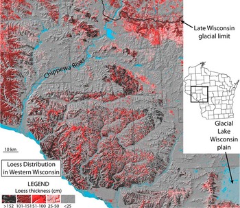
Because most of this landscape is sloping and hence subject to erosion, loess deposits vary greatly in thickness. Many of the loess deposits are spatially disjunct, and many areas lack loess entirely (Schaetzl et al., Reference Schaetzl, Forman and Attig2014; Fig. 3). Where thin, loess deposits are loamy, because they have been intermixed with the underlying residuum. Loess is especially thick on uplands near the Mississippi River (Hole, Reference Hole1976; Scull and Schaetzl, Reference Scull and Schaetzl2011). Much of this loess was likely derived from the valley while it functioned as a major meltwater sluiceway (Leigh and Knox, Reference Leigh and Knox1993; Bettis et al., Reference Bettis, Muhs, Roberts and Wintle2003; Schaetzl et al., Reference Schaetzl, Forman and Attig2014) and from sources farther west. Locally, especially east of the Chippewa River, loess deposits appear to be linked, at least in part, to the Chippewa River valley train (Schaetzl et al., Reference Schaetzl, Forman and Attig2014). Loess deposits farther east are thinner and quite spatially discontinuous (Scull and Schaetzl, Reference Scull and Schaetzl2011; Stanley and Schaetzl, Reference Stanley and Schaetzl2011; Fig. 3). Nonetheless, in preferred sites on stable uplands, loess thicknesses can exceed 3 m, even as nearby landscapes have no detectable loess (Schaetzl et al., Reference Schaetzl, Forman and Attig2014). Often, areas with thin or undetectable amounts of loess occur on sandy side slopes and in lowlands, which may have been unstable during the postglacial permafrost period, and/or which may have acted as a transportation surface for silts (Stanley and Schaetzl, Reference Stanley and Schaetzl2011). In the latter situation, saltating sands impact loess deposits that are accruing, remobilizing them and facilitating their continued transport downwind (Mason et al., Reference Mason, Nater, Zanner and Bell1999; Syverson, Reference Syverson2007). This process continues until a barrier to sand transport is encountered (e.g., a deep river valley, a steep escarpment, or an abrupt upland). Loess then accumulates downwind of the topographic obstruction in the transportation surface.
(color online) Extent and thickness of loess within the study area, as derived from Natural Resources Conservation Service county soil surveys.

METHODS
Loess mapping and sampling
As has been done previously (Stanley and Schaetzl, Reference Stanley and Schaetzl2011; Luehmann et al., Reference Luehmann, Schaetzl, Miller and Bigsby2013; Schaetzl and Attig, Reference Schaetzl and Attig2013), county soil survey data for the study area were downloaded from the Natural Resources Conservation Service, imported into geographic information system (GIS) and rasterized. For soils developed in loess, as described in their official series descriptions (OSDs), we determined the typical loess thickness from the OSDs, entered the value into a GIS attribute table, and used these data to code the GIS map unit symbology. Texture data for the uppermost and deepest mineral horizons were also coded into the GIS. The GIS data were then loaded onto a laptop computer, equipped with GPS, to facilitate field navigation to predetermined, potential sampling sites. Our field sampling goal was to obtain loess samples from numerous broad, stable uplands. Loess was sampled with a hand auger at 223 sites on stable uplands. All samples were obtained within or below the soil profile, but at least ≈30 cm from any underlying sediment or bedrock. We sampled so as to obtain an amalgamated representation of the entire loess column.
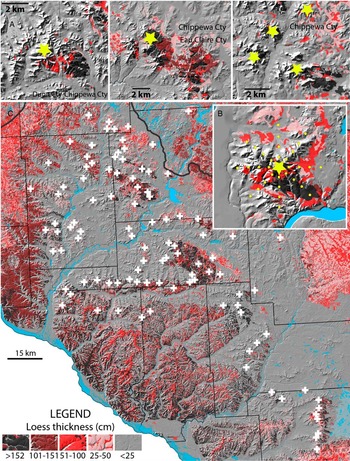
We also used a GIS, in conjunction with NRCS county-level soils data, to evaluate the distribution and thickness of loess deposits near major bedrock inselbergs, ridges, and uplands (Fig. 4). Such data were used to test the hypothesis that loess is preferentially deposited on, primarily, one side of large ridges and isolated uplands. This hypothesis suggests these prominent topographic barriers act as a wind obstruction and, thus, facilitate loess deposition in their lee. Loess should, theoretically, accumulate preferentially on one side of the ridge if the paleowinds that transported the loess originated mainly from one direction (Hesp and Smyth, Reference Hesp and Smyth2017). Similar features, on smaller scales, occur in eolian sand systems, where they are referred to as nebkha or shadow dunes (Hesp, Reference Hesp1981). For each of 104 sites, we estimated loess thickness at distances of 0.5, 1.0, 1.5, and 2.0 km from the ridgetop, along eight cardinal directions, in a GIS (Fig. 4B). Loess thickness were categorized from NRCS county soil data, with ordinal thickness categories as follows: >60inches (5), 40–60 inches (4), 20–40 inches (3), 10–20 inches (1), and sites where loess soils are not mapped (0).
Loess distribution across the study area, showing the locations of sample sites (white crosses) near bedrock uplands. (A) Three representative sites, characteristic of loess distribution near isolated bedrock uplands. Note the much thicker loess on the eastern and southeastern flanks of all of these upland areas. The yellow stars represent the midpoints of the sample grids, as shown in panel B. (B) Another such site, showing the distribution of loess and of sample points used in the geographic information system to estimate loess thickness along eight cardinal directions, at 0.5, 1.0, 1.5, and 2.0 km from the center of the ridge (yellow star). (C) The full distribution of the 104 sample points used to estimate patterns of loess thickness and distribution near isolated bedrock uplands. (For interpretation of the references to color in this figure legend, the reader is referred to the web version of this article.)

Loess and loess data analyses
Loess samples were air-dried, lightly ground to pass a 2 mm sieve, and passed through a sample splitter three times, in order to achieve the homogeneity necessary for laser particle-size diffraction on a Malvern Mastersizer. From each sample, a 2 g subsample was dispersed in a water-based solution of (NaPO3)13⋅Na2O, after shaking for 30 min. As discussed in Miller and Schaetzl (Reference Miller and Schaetzl2012), small subsamples analyzed in laser particle-size analyzers are not always representative. Thus, we analyzed two subsamples from each loess sample and compared the data. In cases where the suite of particle-size data were sufficiently similar statistically, we used the mean values for all subsequent analyses. However, in cases where the data from the two runs were sufficiently dissimilar (for details, see Miller and Schaetzl, Reference Miller and Schaetzl2012), a third, or sometimes fourth, subsample was run, and the two most comparable samples were used to generate the mean values used in subsequent analyses.
Loess deposits are often mixed with underlying sediment, especially in areas known to have had permafrost (McSweeney et al., Reference McSweeney, Leigh, Knox and Darmody1988; Luehmann et al., Reference Luehmann, Schaetzl, Miller and Bigsby2013; Schaetzl and Attig, Reference Schaetzl and Attig2013; Schaetzl and Luehmann, 2013). In our study area, mixing of loess with sandstone residuum below is common, as evidenced by bimodality in the particle-size curves. Therefore, we followed the practice of Luehmann et al. (Reference Luehmann, Schaetzl, Miller and Bigsby2013), and “filtered” the particle-size data (i.e., adjusting the particle sizes by removing the sediment that comprises the coarser “peak” and recalculating the remaining textural data). The goal of the filtering process is to restore the particle-size data as close as possible to the presumed original composition. Because most of our loess samples were from thick deposits, they lacked a second (sand) peak, and the filtering process left the original particle-size data unchanged. Nonetheless, for sites shallow to sandstone residuum, the filtering process performs an important function—restoring the particle-size data of the loess to a condition closer to its original state.
Sandy eolian deposits and landforms
Fieldwork in the study area, associated with several previous studies (Larson et al., Reference Larson, Dryer, Mc Donald, Baker, Running, Faulkner and Jol2008; Olson et al., Reference Olson, Larson, Hupy, Jol, Faulkner and Running2008; Faulkner et al., Reference Faulkner, Larson, Jol, Running, Loope and Goble2016), identified potential sandy eolian deposits and landforms. Particularly, Larson et al. (Reference Larson, Dryer, Mc Donald, Baker, Running, Faulkner and Jol2008) investigated a landform that, based on morphology, internal sedimentary structures, textural analysis, and landscape position adjacent to the Wissota Terrace scarp, was interpreted as a cliff-top parabolic dune. Their work was, however, restricted to this single location (Fig. 2). Olson et al. (Reference Olson, Larson, Hupy, Jol, Faulkner and Running2008) then attempted to identify and map sandy eolian deposits across the region, using NRCS county soils data, concluding that sandy eolian deposits are widespread throughout the LCRV, but the resolution of their predictive mapping left uncertainty regarding the exact distribution and morphology of a variety of such landforms. The studies by both Larson et al. (Reference Larson, Dryer, Mc Donald, Baker, Running, Faulkner and Jol2008) and Olson et al. (Reference Olson, Larson, Hupy, Jol, Faulkner and Running2008) were preliminary investigations, limited in scope, and conducted without the aid of high-resolution light detection and ranging (LIDAR)–derived digital elevation models (DEMs). In the present study, we undertook a more detailed inventory of sandy eolian landforms, based on sand textures (from soil survey data) of landforms with dune-shaped morphologies and by utilizing recently acquired LIDAR data that range in resolution from 0.9 m (3 ft.) to 4.6 m (15 ft.) cell sizes. Dune morphologies were then used to interpret former wind directions. We derived a preliminary chronology of these landforms, based on stratigraphic relationships with other deposits of known age, as well as absolute age control on some archetypical landforms.
Luminescence dating
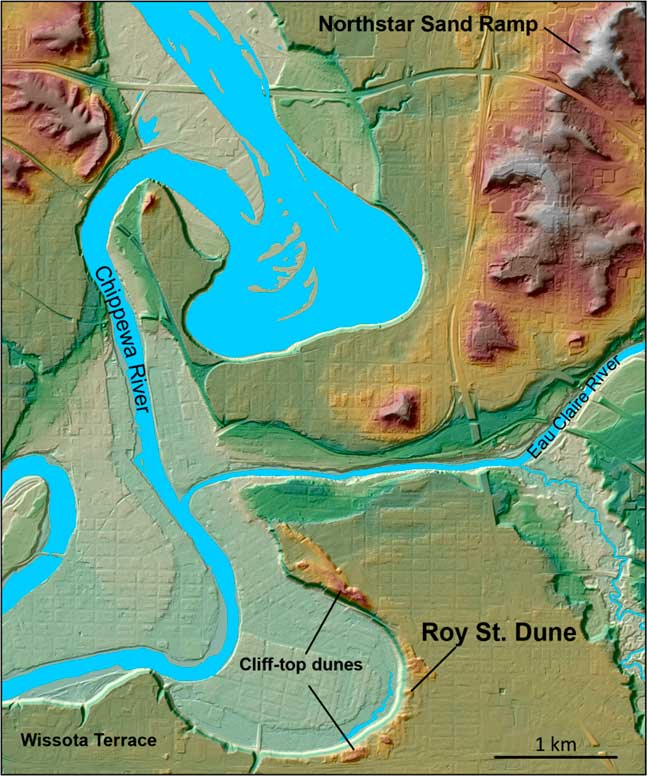
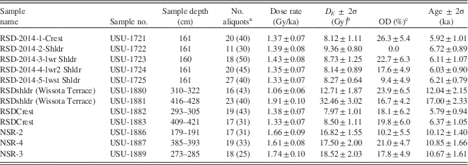
Nine samples were collected from the Roy Street Dune (RSD) for luminescence dating, investigated initially by Larson et al. (Reference Larson, Dryer, Mc Donald, Baker, Running, Faulkner and Jol2008). At the RSD, four samples were collected using a Geoprobe hydraulic coring unit, two from 2.93 to 3.05 m depth and 4.09 to 4.21 m depth at the dune crest, and two at 3.1–3.22 m and 4.16–4.28 m depths from the toe slope. The toe slope samples were collected from the underlying Wissota Terrace fill, to frame the depositional age of the dune within the Chippewa River incision model of Faulkner et al. (Reference Faulkner, Larson, Jol, Running, Loope and Goble2016). Finally, five additional samples were collected at ≈1.6 m depth from a series of hand-dug pits, one each on the crest, shoulder, back slope, foot slope, and toe slope of the dune; we viewed these depths as sufficient to avoid bioturbation issues (Hanson et al., Reference Hanson, Mason, Jacobs and Young2015). Three samples were also recovered using the Geoprobe from the Northstar Sand Ramp (NSR), using a single core, in the middle of the NSR, at depths of 1.79–1.91, 2.73–2.85, and 3.85–3.93 m. Both the RSD and the NSR are located in the city of Eau Claire (Figs. 2 and 5).
(color online) Map of the area near the Northstar Sand Ramp and Roy Street Dune, near the Chippewa River in the city of Eau Claire. Other dunes, also in cliff-top position, atop the Wissota Terrace, are shown. Elevations on this map range from 241 m (Chippewa River) to 334 m.

Sample processing and optically stimulated luminescence (OSL) analyses were conducted at the Utah State University Luminescence Laboratory. Samples were processed to purify the quartz fine sand fraction (150–250 μm) and followed standard procedures involving wet sieving, gravity separation using sodium polytungstate (2.72 g/cm3), and acid treatments with HCl and HF to isolate the quartz component. Samples were analyzed following the latest single-aliquot regenerative-dose procedures (Murray and Wintle, Reference Murray and Wintle2000, Reference Murray and Wintle2003; Wintle and Murray, Reference Wintle and Murray2006), and ages were calculated using the central age model of Galbraith and Roberts (Reference Galbraith and Roberts2012). Data quality criteria included rejection of aliquots with repeat point signals outside of unity (>±10%), signal response in the zero-dose step (>10% of natural signal), and feldspar contamination as indicated by response to infrared stimulation (for similar criteria, see Rittenour et al., 2007). Data from rejected aliquots were not included in equivalent dose, overdispersion, or age calculations. OSL ages are reported at 2σ standard error (Table 1).
Luminescence data for the Roy Street Dune (RSD) and Northstar Sand Ramp (NSR) sites.

a Age analysis using the single-aliquot regenerative-dose procedure of Murray and Wintle (Reference Murray and Wintle2000) on 2 mm small aliquots of quartz sand. Number of aliquots used in age calculation, with number of aliquots analyzed in parentheses.
b Equivalent dose (D E ) calculated using the central age model of Galbraith and Roberts (Reference Galbraith and Roberts2012).
c Overdispersion (OD) represents variance of D E data beyond the measurement uncertainties. OD values >20% may indicate significant scatter due to depositional or postdepositional processes.
Dose-rate calculations were determined by chemical analysis of the U, Th, K, and Rb contents using inductively coupled plasma mass spectrometry and inductively coupled plasma atomic emission spectroscopy techniques and conversion factors from Guerin et al. (Reference Guerin, Mercier and Adamiec2011). The contribution of cosmic radiation to the dose rate was calculated using sample depth, elevation, and latitude/longitude following Prescott and Hutton (Reference Prescott and Hutton1994). Dose rates are calculated based on water content, sediment chemistry, and cosmic contribution (Aitken, 1998).
Ground-penetrating radar
We used ground-penetrating radar (GPR) to examine the internal stratigraphy of the RSD, the NSR, and sand sheets (“reflection facies 1” in Faulkner et al. [Reference Faulkner, Larson, Jol, Running, Loope and Goble2016]). GPR is a noninvasive, shallow geophysical method in which electromagnetic waves are transmitted into the ground and reflected back to the surface from sedimentary boundaries that have contrasting dielectric properties. GPR has been shown to be particularly well suited to sandy eolian deposits (Havholm et al., Reference Havholm, Bergstrom, Jol and Running2003, Jol et al., Reference Jol, Bristow, Smith, Junck and Putnam2003; Baker and Jol, Reference Baker and Jol2007; Bristow, Reference Bristow2009). The details of GPR data collection and interpretation methodologies follow those of Jol and Bristow (Reference Jol and Bristow2003).
The GPR systems used for the study were Sensors and Software pulseEKKO 100 and 1000 with 200 and 225 MHz antennae, respectively. Step size was 0.1 m, with an antennae separation of 0.5 m. Common midpoint surveys collected in the field were analyzed to determine near-surface velocity, which was used to estimate depth of penetration. Topography along the GPR lines was collected using a laser level to geometrically adjust the resulting transect. The profiles were processed using pusleEKKO software, and we applied an automatic gain control, a dewow filter, and trace-to-trace and down-trace averaging to the wiggle trace plot.
RESULTS AND DISCUSSION
Loess patterns and paleowinds
Previous work has concluded that loess in the LCRV was transported mainly by westerly winds from the valley train systems of the Chippewa and Mississippi Rivers (Schaetzl et al., Reference Schaetzl, Forman and Attig2014). The interval for depiction of this loess spans the Late Pleistocene, perhaps peaking between 18 and 13 ka, but likely continuing into the early Holocene (Schaetzl et al., Reference Schaetzl, Forman and Attig2014). The widespread presence of thick, relatively coarse loess on uplands east and south of these two large rivers was given as the main reason for these conclusions. Nonetheless, loess is also often quite thick near isolated bedrock uplands, thinning quickly with distance to the east and southeast. Thus, we speculated that the pattern of loess deposition near such features may provide a more detailed understanding of paleowind directions than would a study of the broader, more “regional” loess patterns. Many of the inselbergs stand isolated within a rolling landscape of sandy sediment, often a mix of residuum, colluvium, alluvium, and eolian sands.
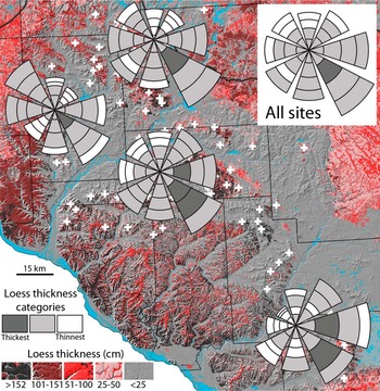
Loess is typically thickest on the east-southeastern sides of the large bedrock inselbergs and ridges in the study area (Figs. 3, 4, and 6). Only in the southern part of the study area, by the uplands immediately west of the glacial Lake Wisconsin plain, is loess usually thickest only on the eastern sides of uplands (Fig. 6). The thickest loess is typically encountered at ≈0.5–1.5 km from the inselberg. Loess deposits on the east-southeastern margins of these inselbergs often exceed 2–3 m in thickness and have likely accumulated over millennia during the Late Pleistocene and early Holocene (Schaetzl et al., Reference Schaetzl, Forman and Attig2014). Loess is often not even mapped in areas that are west, northwest, north, or northeast of such inselbergs, and >1 km distant (Figs. 4A and B). Frequently, soil textures on the west-northwestern flanks of these same uplands are sandy in texture, suggesting that loess was unable to be retained here, perhaps because they were transportation and/or erosion surfaces. Such surfaces may in some instances represent sand ramps—eolian sand that is intermittently being transported up and onto the upland, but usually not over it.
(color online) Loess patterns in the vicinity of bedrock uplands, shown as rose diagrams. Data are shown for all sites combined and for areal subsets. Thicknesses were determined for four distances along eight cardinal directions. Wedge lengths are proportional to the summed average loess thicknesses along the sample points, whereas the grayscale images of each wedge section reflect mean loess thicknesses at that distance from the ridgetop. Some sample sites are covered by the rose diagrams.

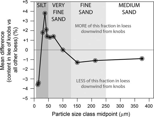
In order to better understand the transportation dynamics of loess near bedrock obstructions, we examined “filtered” textural data for 102 sites that are in the immediate lee (mainly southeast) of such obstructions and compared these data to data for loess from 2224 sites throughout Wisconsin and Michigan’s Upper Peninsula (Schaetzl and Loope 2008, Scull and Schaetzl Reference Scull and Schaetzl2011, Stanley and Schaetzl Reference Stanley and Schaetzl2011, Schaetzl 2012, Luehmann et al. 2013, Schaetzl and Attig Reference Schaetzl and Attig2013, Schaetzl et al. Reference Schaetzl, Forman and Attig2014). These data are from loess that spans a variety of depositional settings (Fig. 7). Loess in the lee of uplands in the study area is comparatively depleted in fine silts and sands, and enriched in medium silts, coarse silts, and the finer sand fractions. This partitioning appears to suggest that finer silts are carried far downwind, whereas all but the finest sand fractions are unable to be transported over the upland. Medium and coarse silts are preferentially deposited in the immediate lee of the ridge. In effect, the uplands act as a “snow fence” for loess, much like isolated plants or patches of vegetation act to force deposition of eolian sand in their lees. The clear orientation of these deposits strongly suggests transport of loess on west and northwest winds.
Mean differences in particle-size concentrations (expressed as percentage of the whole <2 mm “filtered” fraction) for loess at sites in the immediate lee (mainly southeast) of bedrock uplands versus loess at 2224 sites throughout Wisconsin and Michigan’s Upper Peninsula. A value of zero implies that loess in the lee of bedrock uplands is no different, for that fraction, than loess generally across Wisconsin and northern Michigan.

Sand sheets, eolian-dammed drainages, and deflation hollows
Sand sheets are eolian sand deposits characterized by relatively flat or tabular morphologies (Koster, Reference Koster1988; Kasse, Reference Kasse1997; Ritter et al., Reference Ritter, Kochel and Miller2002; Lancaster, Reference Lancaster2009). In cold-climate dune fields, the term sand sheet is used for eolian sand deposits devoid of “dune relief” or slip-face morphologies (Koster, Reference Koster1988). Sand sheets also tend to drape preexisting topography, resulting in the alternative descriptive term “cover sands” (Kasse, Reference Kasse1997).
While establishing an incision chronology of the alluvial deposits of the LCRV, Faulkner et al. (Reference Faulkner, Larson, Jol, Running, Loope and Goble2016) identified a thin (<1.5 m thick) depositional unit of gravel-free sand overlying the highest terraces, including the highest and oldest Wissota Terrace. This deposit, which they referred to as reflection facies 1 based on GPR data, is common both in exposures and GPR imagery. We interpret this sediment, and other texturally and morphologically similar deposits observed throughout the study area, as sand sheets, although in some locations reflection facies 1 may be paleo-overbank deposits.
In the LCRV, sand sheets are discontinuous, but ubiquitous, commonly found on flat to gently sloping outwash plains and treads of the higher fluvial terraces. Visually, they are difficult to interpret. However, textural analysis suggests that they are distinctly different deposits than the glaciofluvial sands and Holocene-aged stream terraces they overlie (Faulkner et al., Reference Faulkner, Larson, Jol, Running, Loope and Goble2016). Sand sheet textures in the LCRV are typically fine sand, loamy fine sand, and loamy sand. More than a dozen soil series descriptions, based on textural characteristics and landscape position, in the Chippewa, Dunn, Pepin, and Eau Claire County soil surveys, are consistent with our sand sheet interpretation (Thomas, Reference Thomas1977; Jakel and Dahl, Reference Jakel and Dahl1989; Meyer, Reference Meyer2002, Reference Meyer2004). Collectively, these series are widespread across the LCRV. The Dunn and Pepin County soil surveys (Meyer, Reference Meyer2002, Reference Meyer2004) explicitly state an eolian origin for sands in the following series: Boplain sand, Chelsea fine sand, Drammen loamy sand, Garne loamy sand, and Plainbo sand.
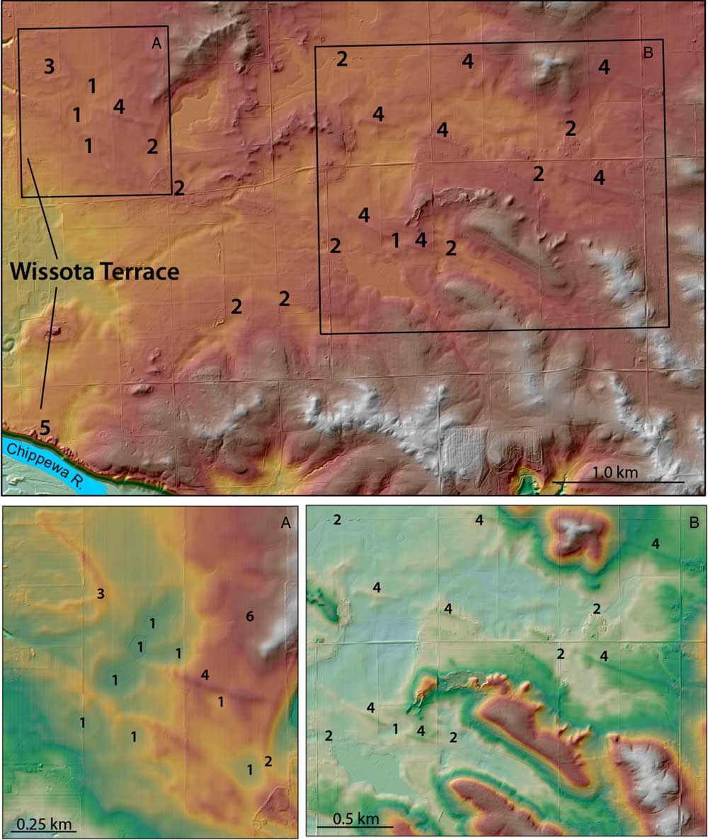
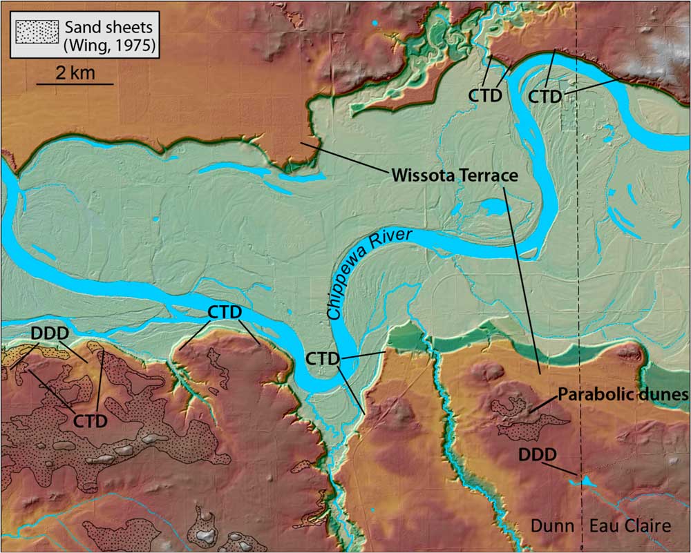
Low-order drainages exiting bedrock uplands are occasionally dammed by sand sheets, forming small lakes/wetlands (Figs. 8 and 9). Characteristic of these eolian-dammed drainages are closed depressions. These depressions, which we interpret to be deflation hollows, are primarily observed on the Wissota Terrace and older outwash surfaces.
(color online) Broad overview maps of eolian features in western Eau Claire County: deflation hollows (1), eolian dammed drainages (2), a parabolic dune (3), linear dunes (4), parabolic dunes in cliff-top position adjacent to the Wissota Terrace scarp (5), and a possible sand ramp (6). Rectangles indicate the extents of panels A and B. Elevations on this map range from 229 m (Chippewa River) to 311 m.

(color online) Sand sheets, parabolic dunes, cliff-top dunes (CTD), and dune-dammed drainages (DDD) present along the Chippewa River near the Dunn County–Eau Claire County border. Dunes are in cliff-top positions adjacent to terrace deposits and overlying pre–Late Wisconsinan glaciofluvial sediment. Note: Soil series descriptions consistent with our eolian sand sheet interpretation are more widespread than the areas identified as sand sheets in the Dunn County soil survey (Meyer, Reference Meyer2004). Similarly, soil series descriptions consistent with our sand sheet interpretation in the Eau Claire County soil survey (Thomas, Reference Thomas1977) are also widespread, but not explicitly identified as such. Elevations on this map range from 221 m (Chippewa River) to 306 m.

Our current understanding of the depositional chronology of sand sheets, eolian-dammed drainages, and deflation hollows is based on spatial and stratigraphic relationships, as well as mapped units of soil series we interpret as having formed in eolian sands. Soils consistent with our sand sheet interpretation are reported in all county soil surveys in the region. Most sand sheet deposits are underlain by sandstone residuum or by outwash deposits associated with pre-Wisconsin glaciations (River Falls Formation) or the Late Wisconsin glaciation (Copper Falls Formation) (Syverson, Reference Syverson2007). This relationship suggests these sands may have been active during the waning stages of the last glacial maximum. Sand sheet deposits underlain by terrace fill within the LCRV confirm that eolian sand mobilization here continued into the early Holocene (Faulkner et al., Reference Faulkner, Larson, Jol, Running, Loope and Goble2016).
Sand sheets, eolian-dammed drainages, and deflation hollows are often located in proximity to other more readily recognized eolian landforms (i.e., parabolic and linear dunes). The latter group of eolian features provides clear insight into paleowind direction, based on their distribution within the LCRV. They become progressively more common to the east and southeast across the region. More locally, eolian-dammed drainages and deflation hollows are commonly, but not exclusively, observed on west- and northwest-facing bedrock slopes that lie to the east and southeast of outwash plains (and locally, sandy till of the River Falls Formation). Deflation hollows are often located immediately west of dunes that dam local drainages. Sand sheets also become progressively thicker (up to 1–2 m thick), as well as more widespread, to the east and southeast in the LCRV. Collectively, these features all suggest that eolian mobilization of sand in the region occurred in response to winds from the west and northwest.
Parabolic dunes
Parabolic dunes are crescent-shaped features that result from a predominant or unidirectional wind regime, with arms usually anchored by vegetation in the upwind direction (Lancaster, Reference Lancaster2009). Parabolic dunes occur throughout the study area, ranging in height from <3 to 20 m (Fig. 8). They are predominantly found on the southern and eastern margins of the LCRV, although they do occur elsewhere, and in proximity to terrace scarps of the Chippewa River (Figs. 8 and 9). Some parabolic dunes are found within or to the southeast or east of sand sheets (Fig. 9). Others occur on outwash plains or sometimes in close proximity to linear dunes. Some irregularly shaped parabolic dunes have coalesced to form ridges, morphologically similar to transverse dune ridges.
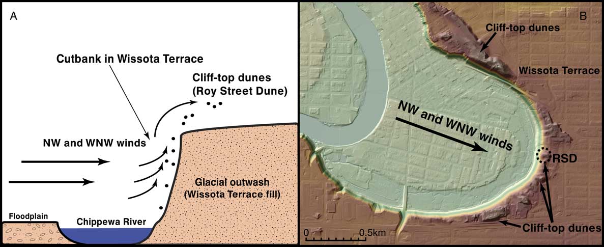
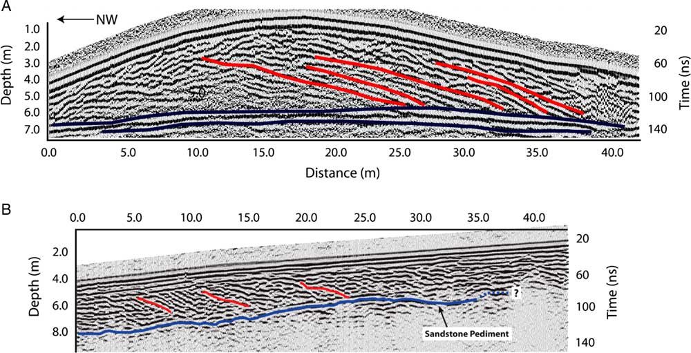
We investigated a typical parabolic dune in Putnam Park, within the city of Eau Claire (Figs. 2 and 10; Larson et al., Reference Larson, Dryer, Mc Donald, Baker, Running, Faulkner and Jol2008). RSD is one of many parabolic dunes (up to 6 m high and 50 m in diameter) that occur immediately adjacent to the scarp of the Wissota Terrace. Initial research revealed that the RSD and those nearby are composed of well-sorted sands, with mean particle sizes in the lower-medium sand fraction (0.25–0.35 mm diameter), consistent with eolian sands. GPR surveys of the RSD also revealed internal structures consistent with migrating slip faces that would have formed on northwesterly winds (Fig. 11). Larson et al. (Reference Larson, Dryer, Mc Donald, Baker, Running, Faulkner and Jol2008) concluded that the RSD and similar landforms are cliff-top (or perched) dunes (Jennings, Reference Jennings1967; Saye et al., Reference Saye, Pye and Clemmensen2006), formed as northwest winds entrained sand exposed in terrace escarpments, as the Chippewa River was actively eroding laterally into Wissota Terrace fill (Fig. 10). Dune growth atop large, sandy escarpments is not uncommon in the region (e.g., Anderton and Loope, Reference Anderton and Loope1995; Arbogast, Reference Arbogast2000).
(color online) Cliff-top dunes in the city of Eau Claire. (A) Model of cliff-top dune formation for the Roy Street Dune (RSD), after Larson et al. (Reference Larson, Dryer, Mc Donald, Baker, Running, Faulkner and Jol2008). Dune-forming winds were best able to entrain sand exposed in the alluvium when the Chippewa River was eroding laterally into terrace fill. (B) Map view of the area near the RSD. Elevations on this map range from 231 (Chippewa River) to 289 m. NW, northwest; WNW, west-northwest.

A 200 MHz ground-penetrating radar (GPR) transect of the Roy Street Dune (A), taken at 0.1 m/ns, and a 225 MHz GPR transect of the Northstar Sand Ramp (B), taken at 0.13 m/ns. Red lines highlight reflection patterns indicative of progressive slip-face migration. Blue lines highlight the contact between dune sediment and alluvium of the Wissota Terrace (Roy Street Dune) or dune sediment and the underlying bedrock (Northstar Sand Ramp). Different shades of blue indicate the strength of the GPR reflections. The lithologic contact below the Wissota Terrace in panel A has multiple horizontal reflections that are clear, so we punctuated that reflection with darker lines. Both GPR transects reveal that these eolian landforms were derived from westerly to west-northwesterly winds. After Larson et al. (Reference Larson, Dryer, Mc Donald, Baker, Running, Faulkner and Jol2008). (For interpretation of the references to color in this figure legend, the reader is referred to the web version of this article.)

Under the cliff-top dune model of Larson et al. (Reference Larson, Dryer, Mc Donald, Baker, Running, Faulkner and Jol2008), the formation of the RSD should be directly linked to processes associated with Chippewa River incision. Based on the time-transgressive incision model of Faulkner et al. (Reference Faulkner, Larson, Jol, Running, Loope and Goble2016), the Chippewa River did not incise below the Wissota Terrace near RSD until sometime after 8.9 ka. This 8.9 ka age is based on OSL ages from a vertical profile of terraces >15 km downstream of the RSD. If the cliff-top model is accurate, this chronology implies that the RSD and other dunes in this area are Holocene-aged landforms.
To test this hypothesis, luminescence dating was conducted on the RSD and in the Wissota Terrace alluvium underlying the RSD (Table 1). The dates from Wissota Terrace alluvium beneath the RSD (RSDshldr Wissota Terrace; Table 1) agree with the long period of glaciofluvial aggradation that largely filled the LCRV in the Late Pleistocene (Faulkner et al., Reference Faulkner, Larson, Jol, Running, Loope and Goble2016). Dates from sites farther downstream indicate that the Wissota Terrace surface remained the active floodplain several thousand years after these dates, later incising (>8.9 ka) and abandoning the Wissota Terrace tread in the vicinity of RSD in the mid-Holocene (Faulkner et al., Reference Faulkner, Larson, Jol, Running, Loope and Goble2016).
The age of the intermediate terraces (T-2 and T-3) located at the base of the Wissota Terrace escarpment (Fig. 10) are unknown at present. Faulkner et al. (Reference Faulkner, Larson, Jol, Running, Loope and Goble2016) identified six terraces in the LCRV below the Wissota Terrace and informally named them T-1 (the lowest) through T-6. According to this naming scheme, the Wissota Terrace would be T-7. Based on the ages of correlated terrace surfaces downstream, the T-3 terrace surface was abandoned sometime after 4.7 ka. However, this does not preclude the area below and near the RSD from being an active channel prior to the formation of the local T-3 terrace surface. Currently, both the local T-2 and T-3 terraces occupy this landscape position, suggesting that this large meander scar may have existed as an active meander through vertical incision events, and older terraces may have been removed during formation of the T-3 meander. Indeed, locally four higher terraces (T-4, T-5, T-6, and Wissota) are in close proximity to this location, pointing to active incision of the Chippewa River near this site (Figs. 2 and 10) from after 8.9 ka through sometime after 4.7 ka, but before 2.3 ka (T-1 terrace). This incision would have exposed alluvium to wind, opening up a sediment source for the RSD and other cliff-top dunes.
The ages of the sands at the RSD crest, shoulder, and foot slope are substantially younger than the Wissota Terrace fill, as expected (Table 1). These dates are tightly clustered, even at depth, between 5.79 and 6.72 ka, suggesting that the RSD stabilized sometime in the mid-Holocene. Further dating of the terraces in this area will help refine this chronology vis-à-vis its connection to the Faulkner et al. (Reference Faulkner, Larson, Jol, Running, Loope and Goble2016) incision model, if the RSD and neighboring dunes are, indeed, cliff-top dunes (Larson et al., Reference Larson, Dryer, Mc Donald, Baker, Running, Faulkner and Jol2008). Alternatively, the RSD may have formed during the dry, warmer conditions of the mid-Holocene, not unlike those recorded regionally (Grigal et al., Reference Grigal, Severson and Goltz1976; Keen and Shane, Reference Keen and Shane1990; Dean et al., Reference Dean, Ahlbrandt, Anderson and Bradbury1996).
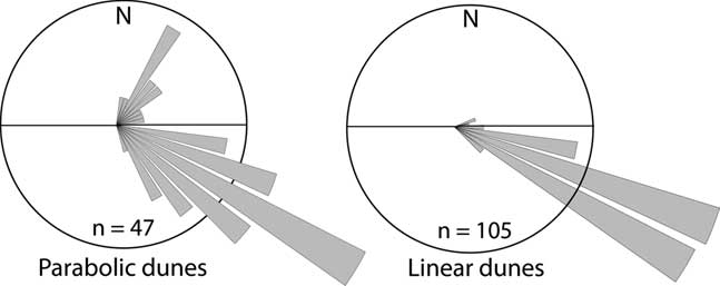
Despite the uncertainty regarding the formation of the RSD, this mid-Holocene–aged parabolic dune can be used infer paleowind direction at the time of deposition (Lancaster, Reference Lancaster2009). At the RSD site, GPR profiles show slip-face orientation indicative of northwest-to-southeast winds (Fig. 11). Parabolic dune orientations elsewhere in the LCRV (Figs. 8, 9, 12, and 13) also point to west-northwesterly and northwesterly winds. We did not use irregularly shaped parabolic dunes (or those that have coalesced into forms morphologically similar to transverse dune ridges) to infer paleowind directionality. Nonetheless, the orientations of those landforms also appear consistent with west-northwesterly and northwesterly winds. The few parabolic dunes that show a southwest-to-northeast orientation are in cliff-top positions adjacent to the Wissota Terrace. Because these dunes are constrained in their formation by the cliff edge, they do not disprove the conclusions drawn previously, for parabolic dunes on the lowlands of the LCRV.
Rose diagrams showing the orientations of parabolic and linear dunes in the study area. Included in this data set are only those parabolic dunes that are sufficiently well preserved to confidently determine orientation.

Linear dunes
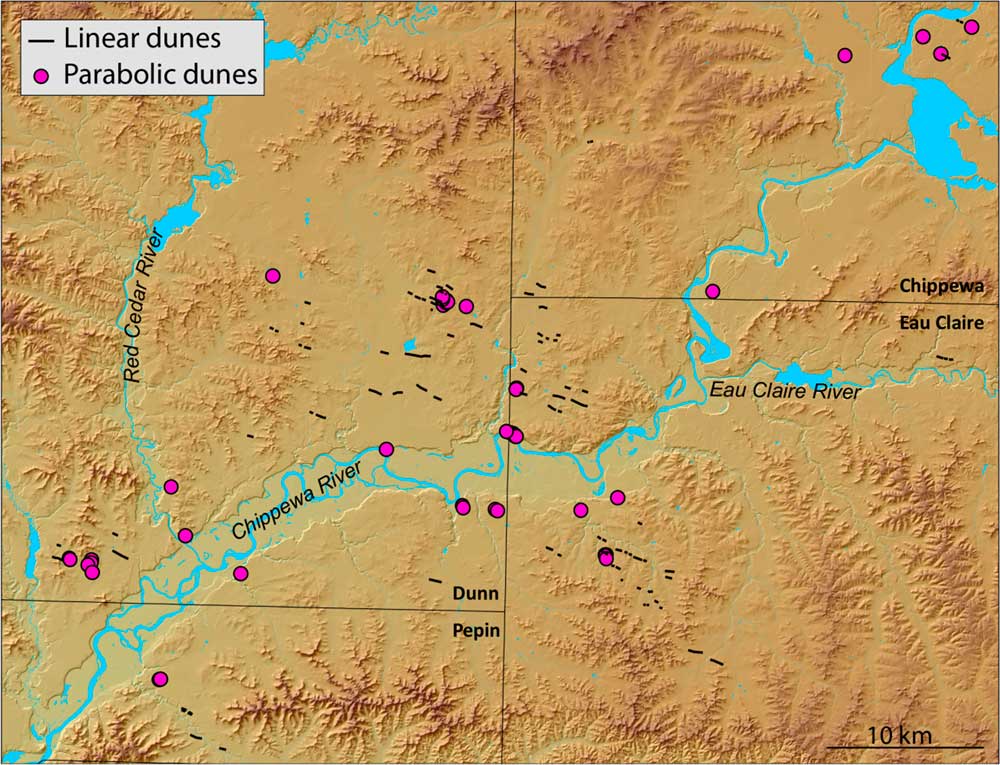
Linear dunes are elongate, eolian depositional forms marked by their parallelism to the direction of net sediment transport (Fryberger and Dean, Reference Fryberger and Dean1979; Lancaster, Reference Lancaster1982, Reference Lancaster2009; Tsoar, Reference Tsoar1989; Livingstone and Warren, 1996; Rubin and Hesp, Reference Rubin and Hesp2009). New LIDAR data for the LCRV brought to light a number of northwest-to-southeast trending linear features that were field checked and interpreted as dunes (Fig. 13). These linear dunes are subtle; most are 1.5–3.0 m high and ≈100 m wide, and many exceed 1 km in length. They are roughly symmetrical in cross section, although some are distinctly asymmetrical, and have generally uniform relief. Their eastern ends often grade smoothly into the adjacent plain. Sometimes, however, they are associated with low, irregular dune forms. In either case, the western ends of the dunes are more sharply defined than the eastern ends. Although not specifically identified in NRCS county soil surveys, the dunes are associated with surface soils texturally consistent with eolian sands.
(color online) The lower Chippewa River valley and adjacent portions of western Wisconsin, showing the locations of major linear and parabolic dunes. The comparatively low resolution of Dunn County LIDAR (light detection and ranging) may explain an apparent lack of linear dunes in that portion of the figure. Only parabolic dunes sufficiently well preserved to determine orientation confidently are shown on this map. Reworked and eroded parabolic dunes and parabolic dunes that have coalesced into a morphology consistent with transverse dunes are not shown. Elevations on this map range from 211 m (Chippewa River) to 400 m.

Our understanding of the age of these linear dunes is informed mainly by stratigraphic relationships. Most of these dunes are underlain by dissected outwash of the River Falls Formation or by Late Wisconsin outwash of the Copper Falls Formation (Syverson, Reference Syverson2007). We know of no such dunes that occur on the Holocene-aged Wissota Terrace, or on treads of younger LCRV terraces, suggesting a Late Pleistocene age.
The linear dunes in the study area all have a broadly northwest-to-southeast orientations (Figs. 12 and 13), suggesting formation by west-northwesterly and northwesterly winds. Well-defined western ends and tapering eastern margins that blend into the surrounding landscape also support this conclusion.
Sand ramps
Few studies have examined sand ramps in environments outside of the contemporary arid zone; only a mention of sand ramps near the Root River, Minnesota, suggests that these forms may be widespread in the upper Midwest, USA (Hanson et al., Reference Hanson, Mason, Jacobs and Young2015). We focused on the NSR (Fig. 5) as a representative form in the LCRV. Sediments at the NSR are dominated by well-sorted, fine to fine-medium loamy sands. Largely devoid of coarse fragments, parts of the sand ramp are nonetheless interbedded with gravelly colluvial debris derived from the bedrock beneath the sand ramp. Visual mineralogical investigations of sand grains in the NSR are consistent with Wissota Terrace fill mineralogy, rather than the uniformly quartz-rich sandstone mineralogy of the bedrock slope and ridge that the NSR overlies. We interpret this mineralogical distinction to indicate that the sands of the NSR accumulated contemporaneously with an active Wissota Terrace outwash surface (i.e., the latter was the source of sands in the NSR).
The three luminescence dates from the NSR, collected approximately halfway up the slope, range from 10.85 to 10.12 ka, indicating a short depositional interval (Table 1). These ages are significantly older than the incision of the Chippewa River that abandoned the Wissota Terrace. The difference in age between the NSR sands and the Chippewa River incision abandoning the Wissota outwash surface, along with the mixed mineralogy of the NSR sediments, points to the Wissota outwash surface as the likely sand source for the NSR.
The location of the NSR suggests transport of sands, up and onto the underlying bedrock slope (pediment), on westerly winds. Additional evidence for west-to-east transport comes from high-angle reflections, recorded in GPR imagery, which we interpret as eastward (and uphill) migrating eolian slip faces (Fig. 11). Finally, as is common at many bedrock uplands in the region, the sands on the western flank of the ridge that underlies the NSR yield to silt-rich loess on the eastern (lee) slope. Based on these data, and the presence of numerous ventifacted boulders on the surfaces of older glacial deposits in the Chippewa valley (Johnson, Reference Johnson1986; Syverson, Reference Syverson2007), we conclude that strong westerly winds concurrently formed the NSR on the west-facing slope and the loess deposits on the east-facing slope. Our field observations indicate that sand ramps like the NSR are ubiquitous in similar landscape positions across the LCRV, as are loess deposits on the lee sides of bedrock uplands (Fig. 3).
CONCLUSIONS
Some areas near the former ice margin in the northern Great Lakes region show on-ground evidence for easterly, or at least widely variable, winds during the Late Pleistocene deglacial period (Vader et al., Reference Vader, Zeman, Schaetzl, Anderson, Walquist, Freiberger, Emmendorfer and Wang2012; Luehmann et al., Reference Luehmann, Schaetzl, Miller and Bigsby2013; Schaetzl and Attig, Reference Schaetzl and Attig2013; Schaetzl et al., Reference Schaetzl, Krist, Luehmann, Lewis and Michalek2016), providing on-the-ground support for the COHMAP model (COHMAP Members, 1988). Despite being immediately south of the former ice front, eolian landforms and sediments in the LCRV show little evidence of having been formed by easterly winds. Instead, eolian landforms and sediments—including dune sand morphology and stratigraphy and loess thicknesses and textures—indicate that eolian systems here were controlled by west-northwesterly and northwesterly winds. These winds were strong enough to (1) form ventifacts; (2) transport sand up and onto the western margins of bedrock uplands, as sand ramps; and (3) transport sand up and onto the tops of cutbanks of the Chippewa River, as clifftop dunes. Particularly impressive is an array of linear and parabolic dunes on the sandy lowlands of the LCRV that also support formation on west-northwesterly and northwesterly winds.
Together, these data paint a picture of a sandy landscape, impacted by loess from western sources, during the Late Pleistocene and into the early Holocene, with a myriad of eolian features forming in the valley proper. The latter include features associated with processes of both eolian erosion and deposition, including subsequent remobilization. Spatially and temporally intermittent transport of eolian sands likely helped to remobilize some of the loess, such that most lowland areas are devoid of loess and are dominated by deflation hollows and various types of small dunes. Much of the remobilized loess was mixed into the underlying sediment or transported out of the region, while some was deposited as thick loess in the lee of bedrock uplands. Further work will help constrain the timing of the eolian systems in the region and therefore better link this suite of eolian activity to the paleoclimatic record.
ACKNOWLEDGEMENTS
We acknowledge support from the Office of Research and Sponsored Programs and Department of Geography at University of Wisconsin–Eau Claire for funding and other resources. We also acknowledge Minnesota State University, Mankato, for financial support. Support for the 2016 LoessFest in Eau Claire, from INQUA’s Commission on Stratigraphy and Chronology and the National Science Foundation to RJS (GSS award 1559045) is also acknowledged; discussions associated with this conference facilitated the development of this paper. Chase Kasmerchak assisted in the development of graphics. We thank Kent Syverson for help and insightful conversations during the course of this research.