1 Introduction
1.1 Objectives of the paper
There is an increasing need to reduce noise radiating from engineering devices. Aeroacoustic noise becomes more and more serious as the moving or rotating speed of devices increases, since the acoustic power of aeroacoustic noise is proportional to
 $M^{5}{-}M^{8}$
, where
 $M$
is the Mach number of the flow or speed of the device, while that of mechanical noise is typically proportional to
 $M^{2}$
. Understanding the generation mechanism of aeroacoustic noise is indispensable for establishing a general method for their reduction. Aeroacoustic analogies that date back to Lighthill (Reference Lighthill1952) have contributed much to the improvement of our understanding. Compared to the success of these aeroacoustic analogies, however, there have been a limited number of methods of sound reduction that are effective and can be applicable generally. Although we know that aeroacoustic noise is reduced by making the surfaces of devices smooth and/or suppressing spanwise vortices, most of them are based on experience and trial and error. Moreover, there are problems in which aeroacoustic analogies are not always accurate: some versions of aeroacoustic analogies assume that the sound source is compact and lose accuracy in non-compact cases or moderate Mach-number flows; more importantly, feedback from the sound on the flow is usually neglected in aeroacoustic analogies. Therefore, further fundamental studies of aeroacoustic sound generation are required.
One of the fundamental problems of practical importance is aeroacoustic noise generation in a time-varying geometry. In particular, devices like wind turbines, helicopters, axial flow fans and other turbomachinery possess not only rotating wings but also fixed parts like towers and struts. Although the aeroacoustic analogy of Ffowcs Williams & Hawkings (Reference Ffowcs Williams and Hawkings1969) has been successful in predicting noise radiated from rotating wings, there is little knowledge for aeroacoustic noise due to relative motion of wings and fixed parts. For example, interaction between the rotating blades and a tower is believed to be responsible for the generation of the low-frequency noise that sometimes causes trouble between residents in the neighbourhood and the electricity companies (McNerney, van Dam & Yen-Nakafuji Reference McNerney, van Dam and Yen-Nakafuji2003).
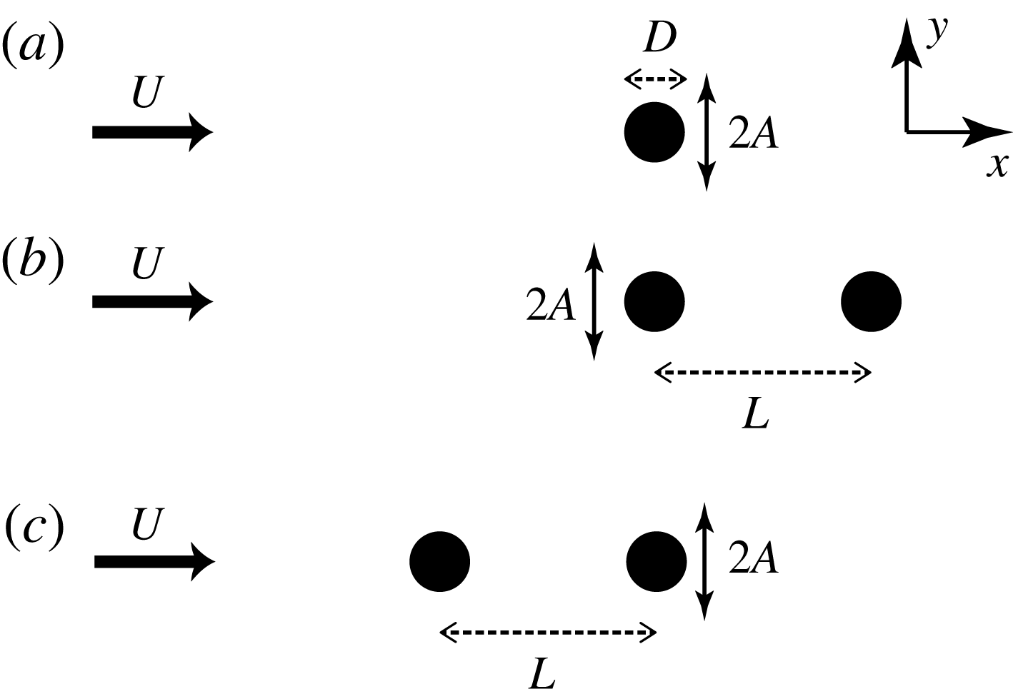
Schematic diagram of flow past an oscillating cylinder and a fixed cylinder.

In this paper, we consider aeroacoustic sound generated in a flow past oscillating and fixed cylinders (figure 1). This problem involves the key ingredients of the aeroacoustic noise generated from the devices listed above: flow, a moving body and a fixed body. Thus it is one of the most fundamental problems of aeroacoustic sound generation in time-varying geometry. Our main objectives are to clarify the mechanism of sound generation in flow in time-varying geometry and to find clues for noise reduction.
1.2 Flow past oscillating and fixed cylinders
The flow past a single oscillating cylinder has been extensively studied as a fundamental problem of vortex–structure interaction (Sarpkaya Reference Sarpkaya1978; Bearman Reference Bearman1984), although most of the works focus on the fluid motion and the aeroacoustic noise has been left untouched. More than half a century ago Bishop & Hassan (Reference Bishop and Hassan1964) studied this experimentally, focusing on the lift and drag forces exerted on an oscillating cylinder. Experimental studies followed by many authors (Koopmann Reference Koopmann1967; Honji & Taneda Reference Honji and Taneda1968; Griffin Reference Griffin1971; Griffin & Ramberg Reference Griffin and Ramberg1974; Zdravkovich Reference Zdravkovich1982; Williamson & Roshko Reference Williamson and Roshko1988; Ongoren & Rockwell Reference Ongoren and Rockwell1989). There are also many numerical works. In particular, two-dimensional low-Reynolds-number flows have been investigated by several authors (Karniadakis & Triantafyllou Reference Karniadakis and Triantafyllou1989; Anagnostopoulos Reference Anagnostopoulos2000a ,Reference Anagnostopoulos b ; Guilmineau & Queutey Reference Guilmineau and Queutey2002; Zheng & Zhang Reference Zheng and Zhang2008). The most important and remarkable finding in these experimental and numerical studies is that the fluid motion depends crucially on the frequency and amplitude of the cylinder oscillation. When the frequency is close to the natural frequency of vortex shedding for a fixed cylinder, the fluid motion synchronizes with the cylinder oscillation (periodic lock-in state); the velocity component at an observation point oscillates periodically with the frequency of the cylinder oscillation. The fluid motion becomes non-periodic when the frequency is out of the range; the dominant frequency of the fluid motion can still be that of cylinder oscillation (non-periodic lock-in state) or can be the natural frequency (non-lock-in state). To be precise, the definition of lock-in state differs among authors. Firstly, some authors take the power spectrum of velocity at one point, while others take that of force. Secondly, some authors regard non-periodic lock-in state as non-lock-in state.
There are a few works on the flow past two cylinders in a tandem arrangement, at least one of which is oscillating. Tanida, Okajima & Watanabe (Reference Tanida, Okajima and Watanabe1973) studied experimentally a flow past a fixed cylinder and an oscillating cylinder behind it. This problem was studied numerically by Li, Sun & Roux (Reference Li, Sun and Roux1991) and Yang & Zheng (Reference Yang and Zheng2010). Mahir & Rockwell (Reference Mahir and Rockwell1996) investigated vortex formation in a flow past two oscillating cylinders experimentally; their work was followed numerically by Papaioannou, Yue & Triantafyllou (Reference Papaioannou, Yue and Triantafyllou2006). These works have revealed that the distance between the cylinders is important, in addition to the mechanisms found in the case of a single oscillating cylinder, which include lock-in and its dependence on the frequency, in the two-cylinder case. However, none of these works has investigated aeroacoustic noise.
1.3 Computational aeroacoustics for complex and time-varying geometry
We investigate the aeroacoustic sound generated in a flow past oscillating and fixed cylinders by direct numerical simulation (DNS), in which the sound pressure is obtained directly as a numerical solution of the compressible Navier–Stokes equations. DNS has some advantages over experiments: in DNS the whole flow field of any physical quantity is easily obtained without background noise as long as the accuracy of the simulation is sufficiently high; in experiments, on the other hand, it is usually difficult to obtain flow field and sound pressure simultaneously and eliminate background noise. Thus the mechanism of sound generation can be pursued with the aid of detailed data of pressure, fluid motion and sound source.
DNS also has advantages over hybrid methods in computational aeroacoustics, in which the sound sources are obtained numerically by solving the incompressible Navier–Stokes equations assuming the flow Mach number to be small and the sound pressure is predicted by aeroacoustic analogies. In the hybrid method, the accuracy of the predicted sound should be carefully addressed since several assumptions including low-Mach-number flow are used in most of the aeroacoustic analogies; more importantly, feedback from sound or the compressible component on the flow cannot be taken into account. In contrast, DNS requires no assumptions and contains all the physics.
In spite of these advantages, DNS has not been used frequently in aeroacoustics since it demands heavy numerical costs and it has been difficult to deal with complex geometry while keeping high accuracy; DNS studies have been limited to rather low-Reynolds-number flows in simple geometry (Colonius & Lele Reference Colonius and Lele2004; Wang, Freund & Lele Reference Wang, Freund and Lele2006). Recently, however, we have shown that the corrected volume penalization (VP) method can resolve aeroacoustic sound generated in complex and time-varying geometry with sufficient accuracy (Komatsu, Iwakami & Hattori Reference Komatsu, Iwakami and Hattori2016). This method is based on the VP method for compressible flow developed by Liu & Vasilyev (Reference Liu and Vasilyev2007) and modified to satisfy Galilean invariance. In Komatsu et al. (Reference Komatsu, Iwakami and Hattori2016) the aeroacoustic sound radiated from a flow past a square cylinder or a circular cylinder which is fixed or oscillating was captured by the corrected VP method; the results were compared to those obtained by a standard method with body-fitted grid systems, and sufficient accuracy was confirmed.
The present problem is challenging in the sense that the geometry is time-varying, as one cylinder oscillates while the other cylinder is fixed. There are serious difficulties in simulating such a problem with a body-fitted grid system: the grid points should move smoothly and one should take care not to lose high accuracy in the deformed grid system. However, the corrected VP method can be applied to the present problem without these difficulties. The present paper will show that the corrected VP method is an effective and useful tool in computational aeroacoustics.
The differences between the present paper and relevant previous papers are pointed out in some detail. First of all, no previous paper except Komatsu et al. (Reference Komatsu, Iwakami and Hattori2016) has considered the aeroacoustic sound generated in the flow past oscillating and fixed cylinders; in fact, just two examples were presented in Komatsu et al. (Reference Komatsu, Iwakami and Hattori2016) to demonstrate the applicability of the corrected VP method; however, the physics of the flow and the aeroacoustic sound was totally untouched. Inoue & Hatakeyama (Reference Inoue and Hatakeyama2002) studied the aeroacoustic sound generated in a flow past a fixed cylinder by DNS; Curle’s acoustic analogy taking account of the Doppler effect was shown to give a good prediction; however, no case with an oscillating cylinder or with multiple cylinders was considered. Li et al. (Reference Li, Sun and Roux1991) studied an incompressible flow past a fixed cylinder and an oscillating cylinder behind it numerically. It should be emphasized that aeroacoustic sound was not considered at all in Li et al. (Reference Li, Sun and Roux1991); although some characteristics of forces, which may give a clue to sound reduction found in the present paper supported by aeroacoustic analogy, were investigated, the dependence of the lift force on the distance between the cylinders, which is crucial for predicting sound, was not considered. Therefore, this paper is the first one that considers the aeroacoustic sound generated in a flow past oscillating and fixed cylinders in detail, shows sound reduction and reveals its mechanism.
1.4 Outline of the paper
This paper is organized as follows. In § 2 the numerical procedure is presented. In § 3 the results of a flow past a single oscillating cylinder are presented, which are needed in determining and discussing the results of the case of two cylinders. In § 4 the flow past an oscillating cylinder in front and a fixed cylinder behind it is considered. The positions of the cylinders are reversed in § 5. We conclude in the final section § 6.
2 Numerical procedure
2.1 Flow model
Three configurations are considered in order to study sound generation from a flow past an oscillating and a fixed cylinder (figure 1). First, a uniform flow past a single oscillating cylinder is investigated, since the results are indispensable not only in understanding the two-cylinder case but also for choosing parameter values (figure 1
a). In the second configuration, a fixed cylinder is added in the wake of the flow past an oscillating cylinder (figure 1
b). In the final configuration, the positions of the cylinders are reversed (figure 1
c). The oscillation of the cylinder is in the cross-flow or
 $y$
direction; it is prescribed as
 $y=A\sin (2\unicode[STIX]{x03C0}f_{c}t)$
. The centre of the oscillation coincides with the origin. The fixed cylinder is placed on the
 $x$
axis. The cylinders are circular and their diameters are the same.
The Reynolds number based on the diameter
 $D$
of the cylinder is fixed to
 $Re=\unicode[STIX]{x1D70C}_{0}UD/\unicode[STIX]{x1D707}=150$
, where
 $\unicode[STIX]{x1D70C}_{0}$
is the density at infinity,
 $U$
is the speed of the uniform flow and
 $\unicode[STIX]{x1D707}$
is the viscosity, which is assumed constant; at this low Reynolds number the fluid motion is known to be nearly two-dimensional, allowing us to cover a large region of parameter space with sufficiently many sets of parameter values. The flow Mach number is fixed to
 $M=U/c_{0}=0.2$
, where
 $c_{0}$
is the speed of sound at infinity; in this low-Mach-number flow the compressibility effects on the vortex motion are weak and the sound source may be regarded as acoustically compact. The other parameters are the frequency
 $f_{c}$
and the amplitude
 $A$
of the cylinder oscillation and the distance between the two cylinders
 $L$
. The values of these parameters depend on the configuration and are described in the corresponding sections. The variables are non-dimensionalized with
 $D$
as the length scale,
 $c_{0}$
as the velocity scale and
 $\unicode[STIX]{x1D70C}_{0}$
as the unit of density. In this normalization the time scale is
 $D/c_{0}$
; however, another time scale
 $D/U$
, which is aerodynamically more relevant, is also used for comparison to incompressible cases. In particular, the cylinder oscillation frequency is non-dimensionalized as
 $Sc=f_{c}D/U$
, where
 $Sc$
is the Strouhal number of the cylinder oscillation.
2.2 Numerical methods
The problem under consideration involves a moving and a fixed rigid body simultaneously. The immersed boundary method is suitable for dealing with such problems numerically. In the present study we intend to capture aeroacoustic sound whose amplitude is much smaller than the pressure at infinity by DNS, which implies that the compressible Navier–Stokes equations should be solved directly with sufficiently high accuracy. To this end, the corrected VP method (Komatsu et al. Reference Komatsu, Iwakami and Hattori2016) is employed. In this method the compressible Navier–Stokes equations are supplemented with penalization terms as
 $$\begin{eqnarray}\displaystyle \frac{\unicode[STIX]{x2202}\unicode[STIX]{x1D70C}}{\unicode[STIX]{x2202}t}+\frac{\unicode[STIX]{x2202}}{\unicode[STIX]{x2202}x_{j}}(\unicode[STIX]{x1D70C}u_{j})=-\left(\frac{1}{\unicode[STIX]{x1D719}}-1\right)\unicode[STIX]{x1D712}\frac{\unicode[STIX]{x2202}}{\unicode[STIX]{x2202}x_{j}}[\unicode[STIX]{x1D70C}(u_{j}-U_{0,j})], & & \displaystyle\end{eqnarray}$$
 $$\begin{eqnarray}\displaystyle \frac{\unicode[STIX]{x2202}\unicode[STIX]{x1D70C}u_{i}}{\unicode[STIX]{x2202}t}+\frac{\unicode[STIX]{x2202}}{\unicode[STIX]{x2202}x_{j}}(\unicode[STIX]{x1D70C}u_{i}u_{j}) & = & \displaystyle -\frac{\unicode[STIX]{x2202}p}{\unicode[STIX]{x2202}x_{i}}+\frac{\unicode[STIX]{x2202}\unicode[STIX]{x1D70F}_{ij}}{\unicode[STIX]{x2202}x_{j}}-\frac{\unicode[STIX]{x1D712}}{\unicode[STIX]{x1D702}}(u_{i}-U_{0,i})\nonumber\\ \displaystyle & & \displaystyle -\,u_{i}\left(\frac{1}{\unicode[STIX]{x1D719}}-1\right)\unicode[STIX]{x1D712}\frac{\unicode[STIX]{x2202}}{\unicode[STIX]{x2202}x_{j}}[\unicode[STIX]{x1D70C}(u_{j}-U_{0,j})],\end{eqnarray}$$
 $$\begin{eqnarray}\displaystyle \frac{\unicode[STIX]{x2202}e}{\unicode[STIX]{x2202}t}+\frac{\unicode[STIX]{x2202}}{\unicode[STIX]{x2202}x_{j}}[(e+p)u_{j}] & = & \displaystyle \unicode[STIX]{x1D705}\frac{\unicode[STIX]{x2202}^{2}T}{\unicode[STIX]{x2202}x_{j}\unicode[STIX]{x2202}x_{j}}+\frac{\unicode[STIX]{x2202}}{\unicode[STIX]{x2202}x_{j}}(\unicode[STIX]{x1D70F}_{ij}u_{i})-\frac{\unicode[STIX]{x1D712}}{\unicode[STIX]{x1D702}_{T}}(T-T_{0})-\frac{\unicode[STIX]{x1D712}}{\unicode[STIX]{x1D702}}(u_{j}-U_{0,j})u_{j}\nonumber\\ \displaystyle & & \displaystyle -\,\frac{1}{2}u_{i}u_{i}\left(\frac{1}{\unicode[STIX]{x1D719}}-1\right)\unicode[STIX]{x1D712}\frac{\unicode[STIX]{x2202}}{\unicode[STIX]{x2202}x_{j}}[\unicode[STIX]{x1D70C}(u_{j}-U_{0,j})],\end{eqnarray}$$
where
 $\unicode[STIX]{x1D70C}$
is the density of the fluid,
 $u_{i}$
is the velocity,
 $p$
is the pressure,
 $\unicode[STIX]{x1D70F}_{ij}=\unicode[STIX]{x1D707}[(\unicode[STIX]{x2202}u_{i}/\unicode[STIX]{x2202}x_{j})+(\unicode[STIX]{x2202}u_{j}/\unicode[STIX]{x2202}x_{i})-(2/3)(\unicode[STIX]{x2202}u_{l}/\unicode[STIX]{x2202}x_{l})\unicode[STIX]{x1D6FF}_{ij}]$
is the viscous stress tensor,
 $e$
is the total energy,
 $T$
is the temperature,
 $U_{0,i}$
and
 $T_{0}$
are the velocity and the temperature of the rigid bodies, respectively,
 $\unicode[STIX]{x1D719}$
is the porosity,
 $\unicode[STIX]{x1D702}$
is the viscous permeability and
 $\unicode[STIX]{x1D702}_{T}$
is the thermal permeability. The terms that are proportional to
 $\unicode[STIX]{x1D712}$
are called penalization terms. The mask function
 $\unicode[STIX]{x1D712}$
, defined as
 $$\begin{eqnarray}\displaystyle \unicode[STIX]{x1D712}(\boldsymbol{x},t)=\left\{\begin{array}{@{}ll@{}}1 & \text{if }\boldsymbol{x}\in \text{rigid bodies},\\ 0 & \text{otherwise},\end{array}\right. & & \displaystyle\end{eqnarray}$$
makes it possible to deal with any complex and/or time-varying geometry in principle, as the boundary conditions at the surface of the rigid bodies, which are the no-slip conditions and the isothermal condition in the present case, are satisfied automatically thanks to the penalization terms. It is pointed out that the mask function varies with time to correctly model the oscillating cylinder. For example,
 $\unicode[STIX]{x1D712}$
is expressed as
 $$\begin{eqnarray}\displaystyle \unicode[STIX]{x1D712}(\boldsymbol{x},t)=H[(D/2)^{2}-x^{2}-(y-A\sin 2\unicode[STIX]{x03C0}f_{c}t)^{2}]+H[(D/2)^{2}-(x-L)^{2}-y^{2}] & & \displaystyle\end{eqnarray}$$
in the second configuration (figure 1
b), where
 $H$
is the Heaviside function. In this case
 $U_{0,i}$
is chosen as
 $$\begin{eqnarray}\displaystyle U_{0,1}=0,\quad U_{0,2}(\boldsymbol{x},t)=\left\{\begin{array}{@{}ll@{}}2\unicode[STIX]{x03C0}f_{c}A\cos 2\unicode[STIX]{x03C0}f_{c}t\quad & |x|<D/2+\unicode[STIX]{x1D716},\\ 0\quad & \text{otherwise},\end{array}\right. & & \displaystyle\end{eqnarray}$$
where
 $\unicode[STIX]{x1D716}$
is a small positive constant satisfying
 $\unicode[STIX]{x1D716}<L-D/2$
, and
 $T_{0}$
is fixed to the temperature of the uniform flow. Note that the expressions of
 $U_{0,i}$
and
 $T_{0}$
are effective only inside the rigid bodies
 $\unicode[STIX]{x1D712}=1$
, where they are set to the velocity and the temperature of the cylinders; it can be arbitrary in the fluid region
 $\unicode[STIX]{x1D712}=0$
since the penalization terms vanish.
As in Komatsu et al. (Reference Komatsu, Iwakami and Hattori2016) a finite difference method is adopted to discretize the above set of equations on a rectangular grid. Spatial derivatives are approximated by the sixth-order-accurate compact scheme (Lele Reference Lele1992) except for the penalization terms, which are approximated by the central finite difference of fourth-order accuracy. For time marching the second-order implicit method is used for the penalization terms, while the second-order Adams–Bashforth method is used for the other terms. The numerical domain and computational grids are also set up as in Komatsu et al. (Reference Komatsu, Iwakami and Hattori2016). Namely, a wide domain
 $|x|,|y|\leqslant 1000D$
is decomposed into four regions of different grid spacings required to resolve the flow: the boundary layer region, the flow region, the sound region and the buffer region. For the details see Komatsu et al. (Reference Komatsu, Iwakami and Hattori2016). Although the numerical accuracy of the corrected VP method is established in Komatsu et al. (Reference Komatsu, Iwakami and Hattori2016), two further tests are performed: (i) the scattering of high-frequency acoustic waves from rigid bodies and (ii) no-slip boundary conditions at the surface of the moving cylinder. See appendices A and B for the results.
The fluid is assumed to be an ideal gas. The Prandtl number
 $Pr=\unicode[STIX]{x1D6FE}\unicode[STIX]{x1D707}/\unicode[STIX]{x1D705}$
is set to 0.72, where the ratio of the specific heats
 $\unicode[STIX]{x1D6FE}$
is set to 1.4. The porosity
 $\unicode[STIX]{x1D719}$
is set to 0.1 and the viscous and thermal permeabilities are set to
 $\unicode[STIX]{x1D702}=\unicode[STIX]{x1D702}_{T}=10^{-4}$
, for which the accuracy has been shown to be sufficient.
2.3 Ffowcs Williams–Hawkings equation in two dimensions
Although the aeroacoustic sound can be obtained as a part of solutions by DNS, it would be important and interesting to compare the results to aeroacoustic analogies. Since the present problems involve a rigid body moving in the flow, we should resort to the Ffowcs Williams–Hawkings equation (Ffowcs Williams & Hawkings Reference Ffowcs Williams and Hawkings1969; Goldstein Reference Goldstein1976) in order to predict the aeroacoustic sound theoretically. In the present case the problem is two-dimensional and the Mach number is small. Thus the sound source may be assumed acoustically compact and the volume integral in the Ffowcs Williams–Hawkings equation is much smaller than the surface integrals. Then in a frame moving with the uniform flow, the Ffowcs Williams–Hawkings equation is reduced to
 $$\begin{eqnarray}\displaystyle \unicode[STIX]{x0394}p=-\frac{1}{4\unicode[STIX]{x03C0}c_{0}}\mathop{\sum }_{\unicode[STIX]{x1D6FC}=o,f}\int _{-\infty }^{\infty }\frac{R_{i}^{(\unicode[STIX]{x1D6FC})}}{C^{(\unicode[STIX]{x1D6FC})}(R^{(\unicode[STIX]{x1D6FC})})^{2}}\frac{\unicode[STIX]{x2202}}{\unicode[STIX]{x2202}\unicode[STIX]{x1D70F}^{(\unicode[STIX]{x1D6FC})}}\left[\frac{F_{i}^{(\unicode[STIX]{x1D6FC})}(\unicode[STIX]{x1D70F}^{(\unicode[STIX]{x1D6FC})})-\unicode[STIX]{x1D70C}_{0}S_{0}A_{i}^{(\unicode[STIX]{x1D6FC})}(\unicode[STIX]{x1D70F}^{(\unicode[STIX]{x1D6FC})})}{C^{(\unicode[STIX]{x1D6FC})}}\right]\text{d}z, & & \displaystyle\end{eqnarray}$$
where
 $\unicode[STIX]{x1D6FC}=o$
and
 $f$
denote the oscillating and fixed cylinders, respectively,
 $\boldsymbol{R}^{(\unicode[STIX]{x1D6FC})}=\boldsymbol{x}-\boldsymbol{X}^{(\unicode[STIX]{x1D6FC})}(\unicode[STIX]{x1D70F})$
is the relative position of the observation point, with
 $\boldsymbol{X}^{(\unicode[STIX]{x1D6FC})}$
being the motion of the centre of the cylinder,
 $$\begin{eqnarray}\displaystyle C^{(\unicode[STIX]{x1D6FC})}=1-\frac{\boldsymbol{V}^{(\unicode[STIX]{x1D6FC})}}{c_{0}}\boldsymbol{\cdot }\frac{\boldsymbol{R}^{(\unicode[STIX]{x1D6FC})}}{R^{(\unicode[STIX]{x1D6FC})}} & & \displaystyle\end{eqnarray}$$
is the Doppler factor with
 $\boldsymbol{V}^{(\unicode[STIX]{x1D6FC})}=\text{d}\boldsymbol{X}^{(\unicode[STIX]{x1D6FC})}/\text{d}\unicode[STIX]{x1D70F}^{(\unicode[STIX]{x1D6FC})}$
being the speed of the cylinder and
 $\unicode[STIX]{x1D70F}^{(\unicode[STIX]{x1D6FC})}=t-R^{(\unicode[STIX]{x1D6FC})}/c_{0}$
is the retarded time. The force exerted on each cylinder is denoted by
 $\boldsymbol{F}^{(\unicode[STIX]{x1D6FC})}$
, while the fictitious force
 $-\unicode[STIX]{x1D70C}_{0}S_{0}\boldsymbol{A}^{(\unicode[STIX]{x1D6FC})}$
, where
 $S_{0}$
is the area of the cylinder and
 $\boldsymbol{A}^{(\unicode[STIX]{x1D6FC})}=\text{d}\boldsymbol{V}^{(\unicode[STIX]{x1D6FC})}/\text{d}\unicode[STIX]{x1D70F}^{(\unicode[STIX]{x1D6FC})}$
, is due to the volume displacement effects and vanishes for the fixed cylinder; we call this fictitious force the inertial force since it may be interpreted as the force required to move the oscillating cylinder filled with the fluid density and is subtracted from the force
 $\boldsymbol{F}^{(o)}$
. In (2.7) the flow is regarded as a three-dimensional flow which is uniform in the
 $z$
direction, as often done in acoustics in two dimensions. In evaluating the retarded time, the motion of the oscillating cylinder is neglected since the amplitude is small:
 $\unicode[STIX]{x1D70F}\approx t-|\boldsymbol{x}-U\boldsymbol{e}_{x}\unicode[STIX]{x1D70F}|$
, where
 $\boldsymbol{e}_{x}$
is the unit vector along the
 $x$
direction.
In the results shown below, (2.7) is used without further approximations for prediction by aeroacoustic analogies. Validation of (2.7) is given in appendix C, where effects of further possible approximations are also checked.
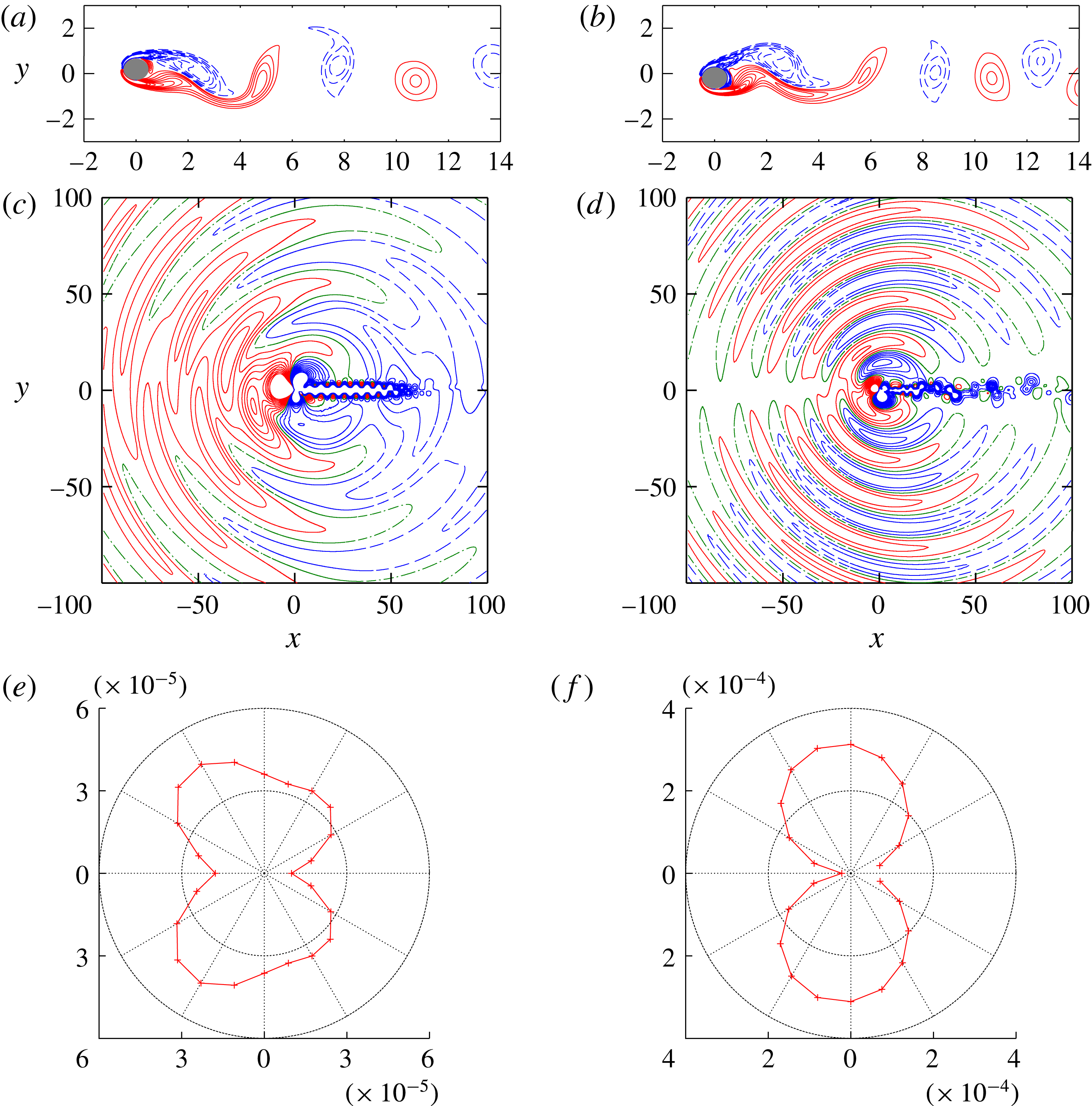
Basic features of vortex motion and sound propagation for a single oscillating cylinder: (a,b) contours of vorticity, (c,d) contours of sound pressure and (e,f) directivity of sound. Here
 $A/D=0.2$
and (a,c)
 $Sc=0.15,~t^{\ast }=181.6$
, and (b,d)
 $Sc=0.22,~t^{\ast }=194.4$
. Contour levels are: (a,c)
 $\unicode[STIX]{x1D714}=\pm 0.1,\pm 0.2,\ldots ,\pm 1$
; and (b,d)
 $\unicode[STIX]{x0394}p=0,\pm p^{\prime },\ldots ,\pm 10p^{\prime }$
with (b)
 $p^{\prime }=4\times 10^{-5}$
and (d)
 $p^{\prime }=2\times 10^{-4}$
. Solid and dashed lines show positive and negative values, respectively, while dot-dashed lines correspond to zero.

3 Flow past a single oscillating cylinder
In this section we investigate aeroacoustic sound generation in a flow past a single oscillating cylinder, which gives a basis for investigating and understanding the case of two cylinders. The amplitude of cylinder oscillation is chosen as
 $A/D=0$
, 0.2 and 0.5. For the fixed case
 $A/D=0$
, the Strouhal number of vortex shedding is
 $St=fD/U=0.18349$
. The frequency of cylinder oscillation is varied within
 $0.1\leqslant Sc\leqslant 0.25$
.
3.1 Vortex motion and sound propagation
Figure 2 shows some features of vortex motion and sound propagation for two different values of cylinder oscillation frequency
 $Sc=0.15$
and 0.22 with
 $A/D=0.2$
. The
 $y$
position of the cylinder is
 $y=A=0.2D$
at
 $t^{\ast }=181.6$
for
 $Sc=0.15$
and
 $y=-A=-0.2D$
at
 $t^{\ast }=194.4$
for
 $Sc=0.22$
, where
 $t^{\ast }=Ut/D$
. Sound pressure is simply defined as
 $\unicode[STIX]{x0394}p=p-p_{0}$
, where
 $p_{0}$
is the pressure at infinity. Vortices are seen to be shed into the wake of the oscillating cylinder as expected in low-Reynolds-number flows past blunt bodies. For
 $Sc=0.15$
the vortex motion is periodic, as can be inferred from the nearly equal distances between the neighbouring vortices shed behind the cylinder. On the other hand, the distance between the vortices is not constant for
 $Sc=0.22$
as the vortex motion is not periodic. These features are consistent with previous results (Anagnostopoulos Reference Anagnostopoulos2000b
; Zheng & Zhang Reference Zheng and Zhang2008).
Acoustic waves are seen to propagate nearly cylindrically in figure 2(c,d). For
 $Sc=0.22$
the directivity of the acoustic waves is similar to that of dipolar sound in a flow past a fixed cylinder (Inoue & Hatakeyama Reference Inoue and Hatakeyama2002) as shown in figure 2(f). For
 $Sc=0.15$
, however, a little discrepancy from the dipolar directivity is observed (figure 2
e); in this case, sound reduction occurs as shown below so that the dipolar sound due to the lift force, which is usually dominant, is weakened and the dipolar sound due to the drag force and the quadrupolar sound become relatively important. The wavelength of the acoustic waves is larger for
 $Sc=0.15$
than for
 $Sc=0.22$
since it is approximately proportional to
 $Sc^{-1}$
.
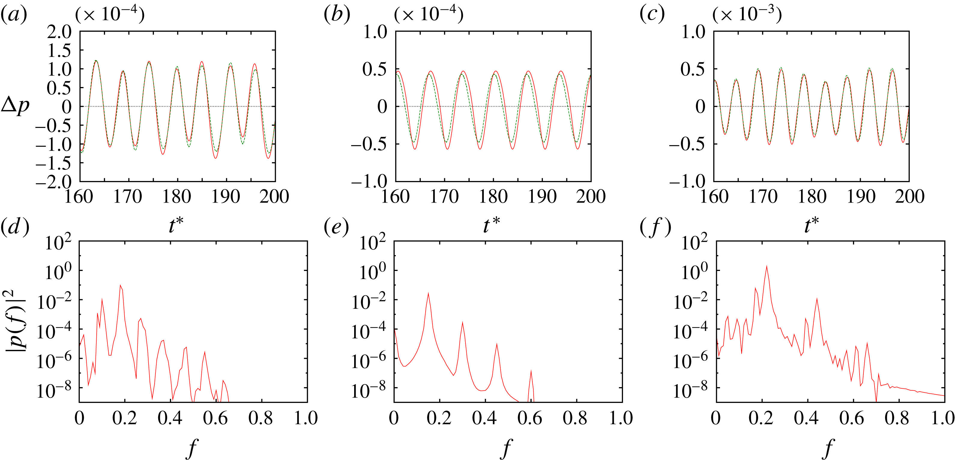
Figure 3 shows the time history of sound pressure at
 $(r/D,\unicode[STIX]{x1D703})=(80,90^{\circ })$
and its spectrum for
 $Sc=0.1$
, 0.15 and 0.22. It is periodic for
 $Sc=0.15$
and non-periodic or modulated for
 $Sc=0.1$
and 0.22. There is one fundamental frequency
 $f=Sc$
for
 $Sc=0.15$
as shown in the spectrum (figure 3
e), while there are two fundamental frequencies
 $f=Sc$
and
 $f=St=0.18349$
for
 $Sc=0.1$
and 0.22 (figure 3
d,f). This shows that the flow synchronizes with the cylinder oscillation for
 $Sc=0.15$
, but does not for
 $Sc=0.1$
and 0.22. Also shown in the time history is the prediction by the Ffowcs Williams–Hawkings equation (2.7), which is in good agreement with the DNS result. In the following we use the power spectrum of sound pressure at
 $(r/D,\unicode[STIX]{x1D703})=(80,90^{\circ })$
to classify lock-in states.
(a–c) Time history and (d–f) spectrum of sound pressure at
 $(r/D,\unicode[STIX]{x1D703})=(80,90^{\circ })$
. Single oscillating cylinder with
 $A/D=0.2$
. (a,d)
 $Sc=0.1$
(non-lock-in), (b,e)
 $Sc=0.15$
(periodic lock-in) and (c,f)
 $Sc=0.22$
(non-periodic lock-in).

The range of
 $Sc$
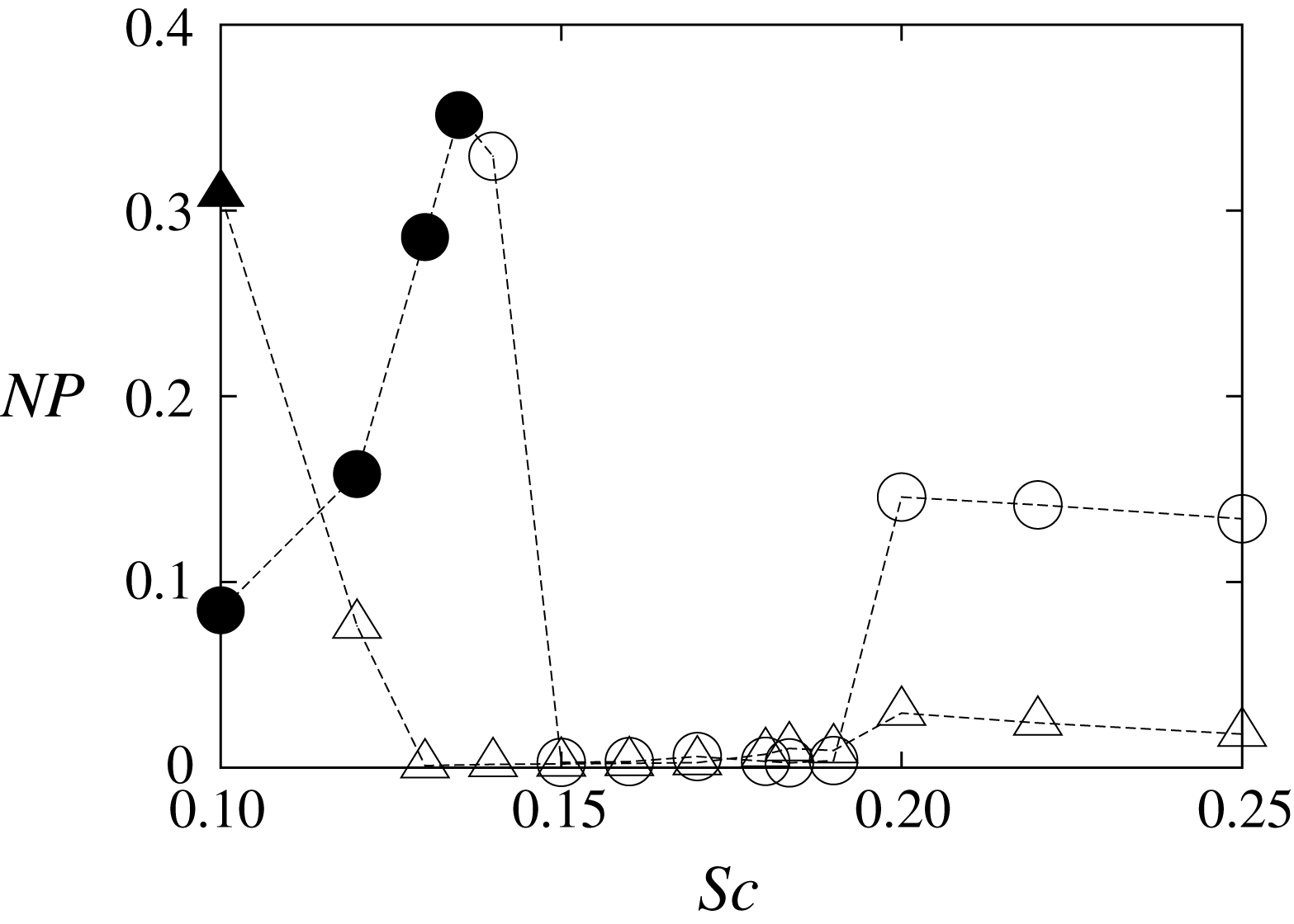
in which lock-in occurs is shown in figure 4, where
 $NP$
is the normalized standard deviation of local maxima of the sound pressure defined as
 $$\begin{eqnarray}\displaystyle NP=\frac{\langle (p_{loc.max.}-\langle p_{loc.max.}\rangle )^{2}\rangle ^{1/2}}{\langle p_{loc.max.}\rangle }. & & \displaystyle\end{eqnarray}$$
Here
 $p_{loc.max.}$
denotes a local maximum of the time history of sound pressure at
 $(r/D,\unicode[STIX]{x1D703})=(80,90^{\circ })$
for
 $120\leqslant t^{\ast }\leqslant 200$
. When the sound pressure is completely periodic, as in figure 3(b),
 $NP$
vanishes since
 $p_{loc.max.}$
is constant;
 $NP>0$
when the sound pressure is non-periodic, as in figure 3(a,c). The open symbols indicate that
 $Sc$
is the dominant frequency implying lock-in, while the solid symbols indicate that
 $Sc$
is subdominant (non-lock-in state). Figure 4 shows that lock-in occurs for
 $Sc/St\geqslant 0.14/0.18349\approx 0.76$
and
 $Sc/St\geqslant 0.12/0.18349\approx 0.65$
when
 $A/D=0.2$
and
 $A/D=0.5$
, respectively; periodic lock-in occurs for
 $0.82\leqslant Sc/St\leqslant 1.04$
and
 $0.71\leqslant Sc/St\leqslant 1.04$
when
 $A/D=0.2$
and
 $A/D=0.5$
, respectively. These results are consistent with previous works: Anagnostopoulos (Reference Anagnostopoulos2000a
) showed that the lock-in region is
 $0.8\lesssim Sc/St\lesssim 1.2$
for a smaller Reynolds number
 $Re=106$
with
 $A/D=0.2$
; although we could not obtain the upper bound of the lock-in region, the lower bounds are close; the lock-in region widens as the amplitude increases, as shown in Karniadakis & Triantafyllou (Reference Karniadakis and Triantafyllou1989).
Normalized standard deviation of local maxima of time history of sound pressure at
 $(r/D,\unicode[STIX]{x1D703})=(80,90^{\circ })$
. Single oscillating cylinder. Circles,
 $A/D=0.2$
; triangles,
 $A/D=0.5$
. The open symbols indicate that
 $Sc$
is the dominant frequency (implying lock-in), while the solid symbols indicate that
 $Sc$
is subdominant (non-lock-in state).

Acoustic power plotted against cylinder oscillation frequency. Single oscillating cylinder. Solid line and
 $+$
,
 $A/D=0.2$
; dashed line and
 $\times$
,
 $A/D=0.5$
. The dot-dashed line shows the acoustic power for a fixed cylinder (
 $A/D=0$
).

3.2 Sound reduction due to synchronization
In this subsection we investigate how acoustic power depends on the cylinder oscillation frequency. In particular, synchronization is shown to lead to reduction of the acoustic power.
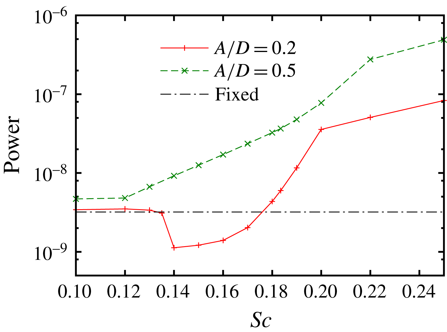
In figure 5 acoustic power is plotted against the cylinder oscillation frequency for two values of oscillation amplitude
 $A/D=0.2$
and 0.5. Acoustic power is obtained by integrating the square of the root-mean-square (r.m.s.) amplitude of sound pressure over
 $\unicode[STIX]{x1D703}$
at
 $r/D=80$
. For
 $A/D=0.2$
it is nearly constant for
 $Sc\leqslant 0.13$
; as
 $Sc$
increases, it suddenly drops at
 $Sc=0.14$
; then it increases monotonically, while the rate of increase is large for
 $0.17\lesssim Sc\leqslant 0.2$
. The curve for
 $A/D=0.2$
is divided into two regions: (i)
 $0.14\leqslant Sc\leqslant 0.2$
and (ii) the rest
 $Sc<0.14$
and
 $Sc>0.2$
. In the former region periodic lock-in to the cylinder oscillation occurs except at the boundary values
 $Sc=0.14$
and 0.2. In this region the acoustic power is much smaller than that inferred by interpolation of the results for
 $Sc<0.14$
and
 $Sc>0.2$
. It is smaller than the case of fixed cylinder (
 $A/D=0$
) for
 $0.14\leqslant Sc\leqslant 0.17$
, the minimum at
 $Sc=0.14$
being 35 % of the fixed-cylinder case. Thus, synchronization contributes to reduction of the acoustic power. For
 $A/D=0.5$
, however, reduction due to synchronization is relatively weak since large oscillation of the cylinder itself produces strong sound as shown below.
Magnitude of force and phase difference. Single oscillating cylinder. The magnitude is the r.m.s. amplitude of the lift coefficients (the force divided by
 $(1/2)\unicode[STIX]{x1D70C}_{0}U^{2}D$
). The phase difference
 $\unicode[STIX]{x0394}\unicode[STIX]{x1D719}$
is that between the force exerted on the oscillating cylinder
 $F_{y}^{(o)}$
and the inertial force
 $-\unicode[STIX]{x1D70C}_{0}S_{0}a_{y}$
. Solid line and
 $+$
,
 $F_{y}^{(o)}$
; dashed line and
 $\times$
,
 $-\unicode[STIX]{x1D70C}_{0}S_{0}a_{y}$
; dotted line and ○, the total force. (a)
 $A/D=0.2$
, (b)
 $A/D=0.5$
.

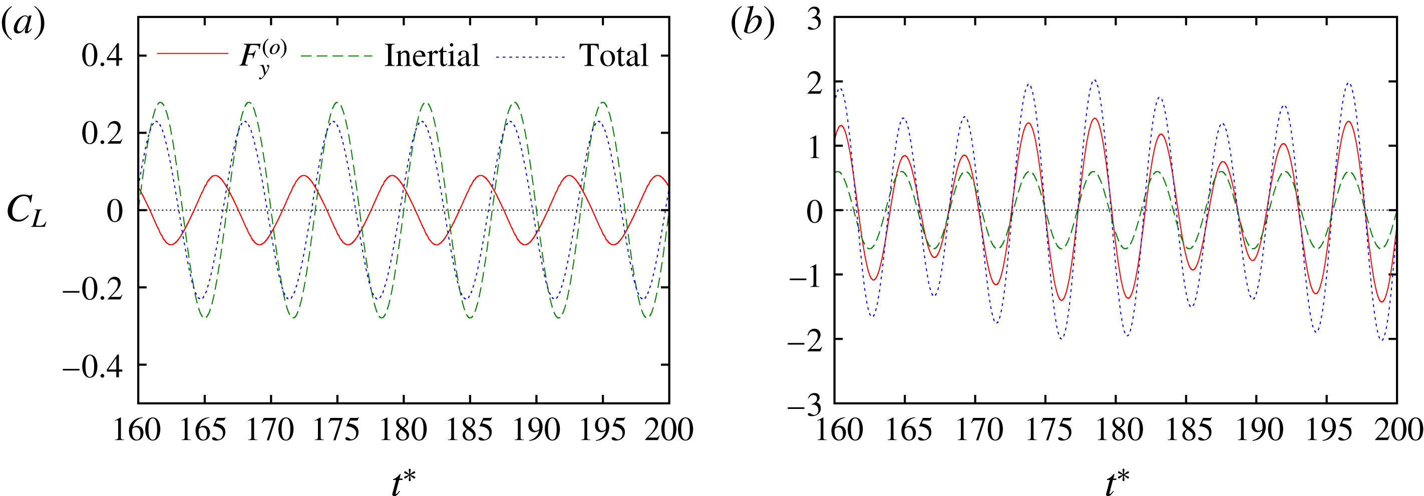
Time history of forces (lift coefficients). Single oscillating cylinder with
 $A/D=0.2$
. Solid line,
 $F_{y}^{(o)}$
; dashed line,
 $-\unicode[STIX]{x1D70C}_{0}S_{0}a_{y}$
; dotted line, the total force. (a)
 $Sc=0.15$
, (b)
 $Sc=0.22$
.

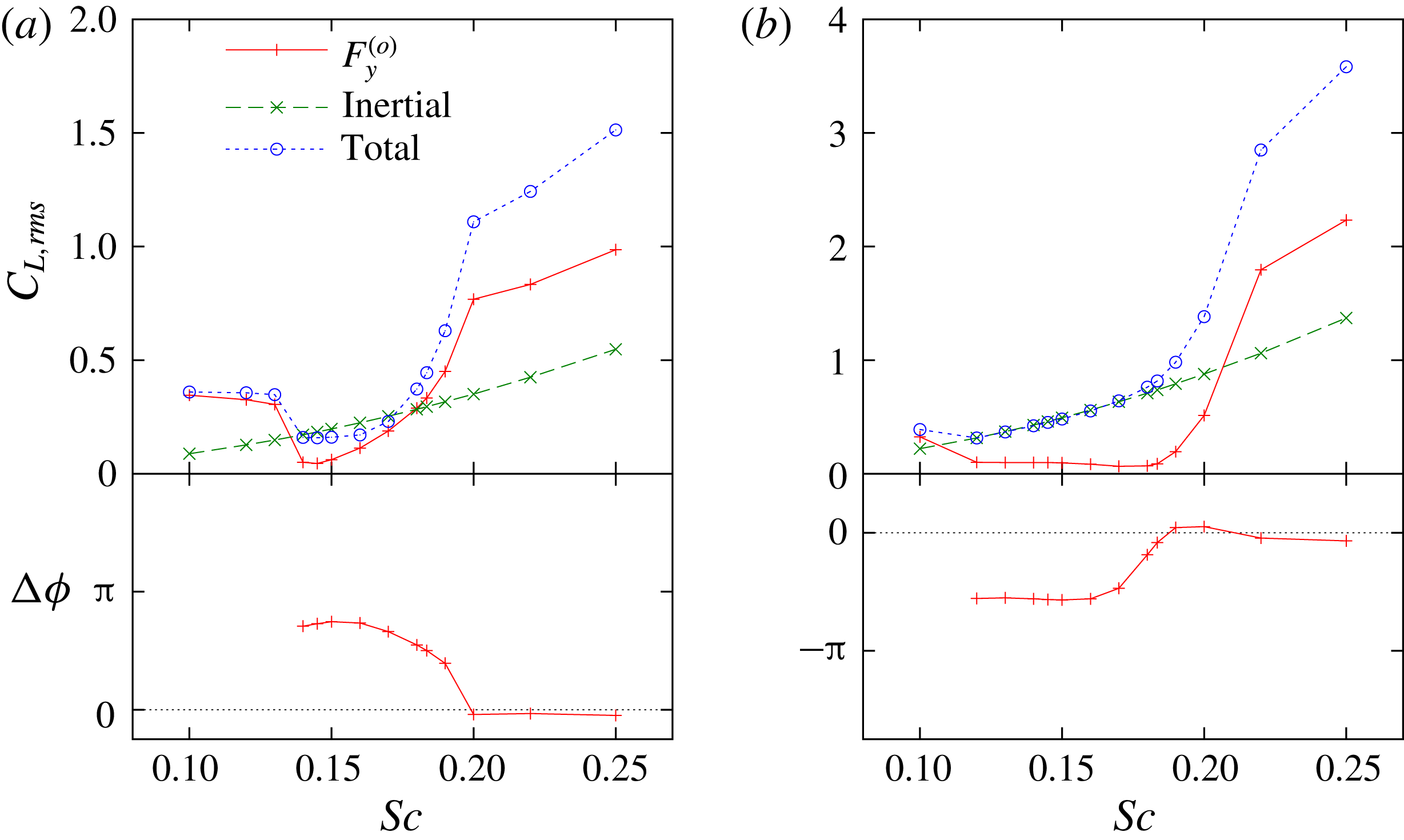
The mechanism of the acoustic power reduction can be understood by using the Ffowcs Williams–Hawkings equation. Figure 6 shows the normalized amplitudes or lift coefficients of the lift force
 $F_{y}^{(o)}$
exerted on the cylinder and the inertial force
 $-\unicode[STIX]{x1D70C}_{0}S_{0}a_{y}$
due to the volume displacement effect, which is proportional to
 $Sc^{2}$
, together with the phase difference between the two forces; here the phases of the forces are those of the Fourier mode
 $f=Sc$
, which is dominant for
 $Sc\geqslant 0.14$
(figure 7). The dependence of the phase difference on the oscillation frequency
 $A/D=0.2$
is similar to that observed in Guilmineau & Queutey (Reference Guilmineau and Queutey2002) for a higher Reynolds number
 $Re=185$
. Comparing with figure 5 it is now evident that reduction of the lift force is responsible for the acoustic power reduction; the lift force is approximately 30 % of the inertial force for
 $0.14\leqslant Sc\leqslant 0.15$
. This reduction is mostly due to lock-in to smaller frequency
 $Sc$
from the natural frequency
 $St$
and partly due to change in flow patterns (Anagnostopoulos Reference Anagnostopoulos2000b
; Guilmineau & Queutey Reference Guilmineau and Queutey2002). It is noteworthy that the phase difference is approximately
 $0.73\unicode[STIX]{x03C0}$
for
 $0.14\leqslant Sc\leqslant 0.17$
, where the acoustic power reduction is significant, so that the total force is smaller than the inertial force. Therefore, periodic lock-in to the cylinder oscillation reduces the lift force and thereby the acoustic power.
For
 $A/D=0.5$
, on the other hand, the inertial force is large, as it is proportional to
 $A$
; in fact it is larger than
 $F_{y}^{(o)}$
for
 $0.12\leqslant Sc\leqslant 0.2$
. The acoustic power due to inertial force is
 $(0.5/0.2)^{2}=6.25$
times larger than that for
 $A/D=0.2$
. As a result acoustic power is not reduced very much, although the lift force itself is significantly reduced in the periodic lock-in state (
 $0.13\leqslant Sc\leqslant 0.19$
).
4 Flow past oscillating and fixed cylinders
Next, we consider the sound generation from flow past an oscillating and a fixed cylinder; the fixed cylinder is placed behind the oscillating cylinder as shown in figure 1(b). The amplitude of cylinder oscillation is fixed to
 $A/D=0.2$
; at this amplitude, significant reduction of acoustic power was observed in the case of a single oscillating cylinder, while the cylinder oscillation itself turned out to be the major source of sound at
 $A/D=0.5$
; therefore, it would be worth pursuing possible combined effects of the cylinder oscillation and the presence of the fixed cylinder at
 $A/D=0.2$
. The frequency of cylinder oscillation is chosen as
 $Sc=0.14$
at which the reduction of acoustic power is nearly most significant, the natural frequency of vortex shedding
 $St=0.18349$
, and 0.22 at which the acoustic power is not reduced very much. The distance between the two cylinders is varied within
 $1.3\leqslant L/D\leqslant 6.0$
.
4.1 Vortex motion and sound propagation
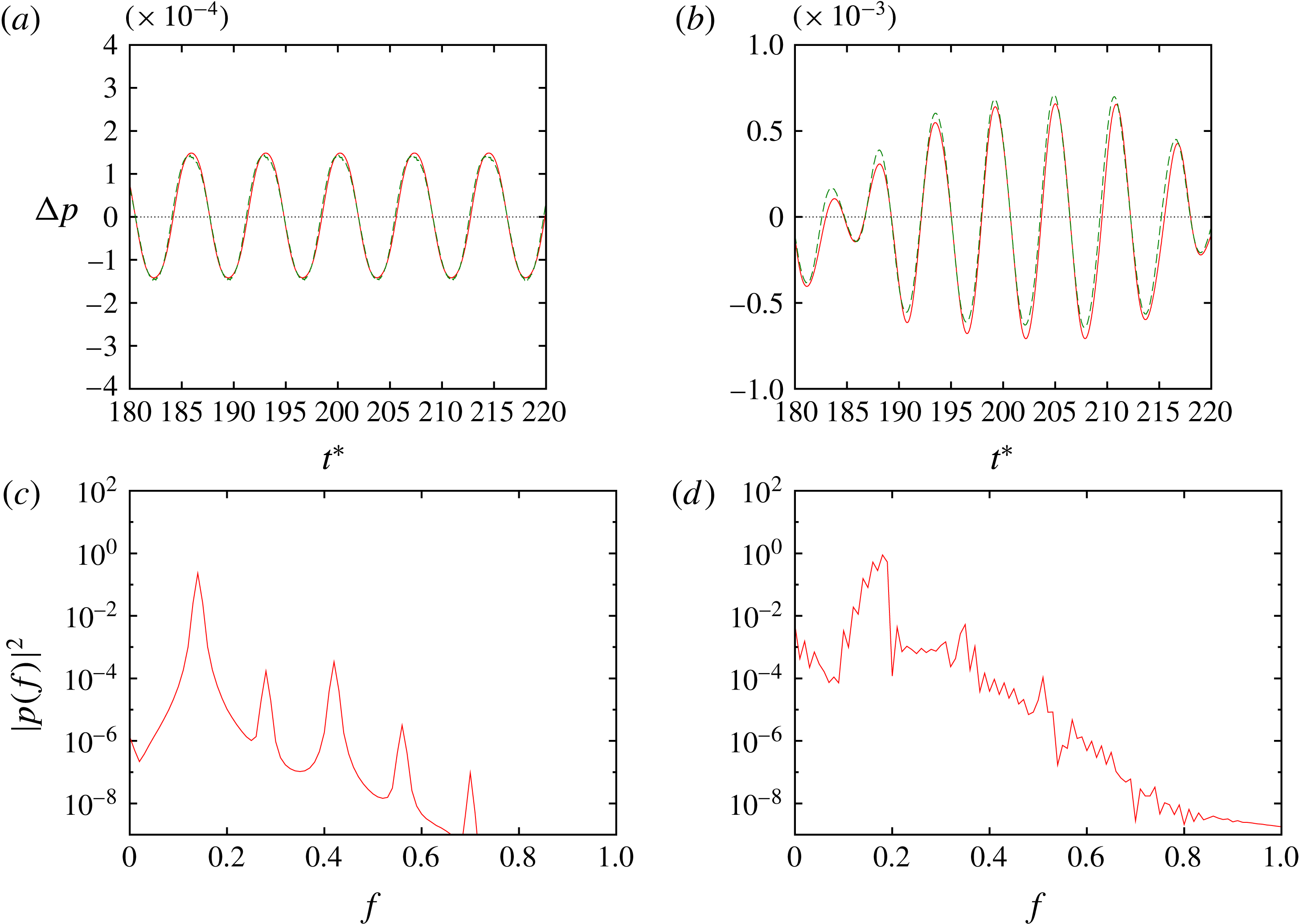
As in the case of the single oscillating cylinder, synchronization with the cylinder oscillation occurs depending not only on the cylinder oscillation frequency but also on the distance between the cylinders. The basic features of vortex motion and sound generation depend on whether the flow is periodic or not. Figure 8 shows an example of periodic lock-in states (
 $Sc=0.14$
and
 $L/D=2.0$
) and an example of non-periodic lock-in states (
 $Sc=0.18349$
and
 $L/D=4.0$
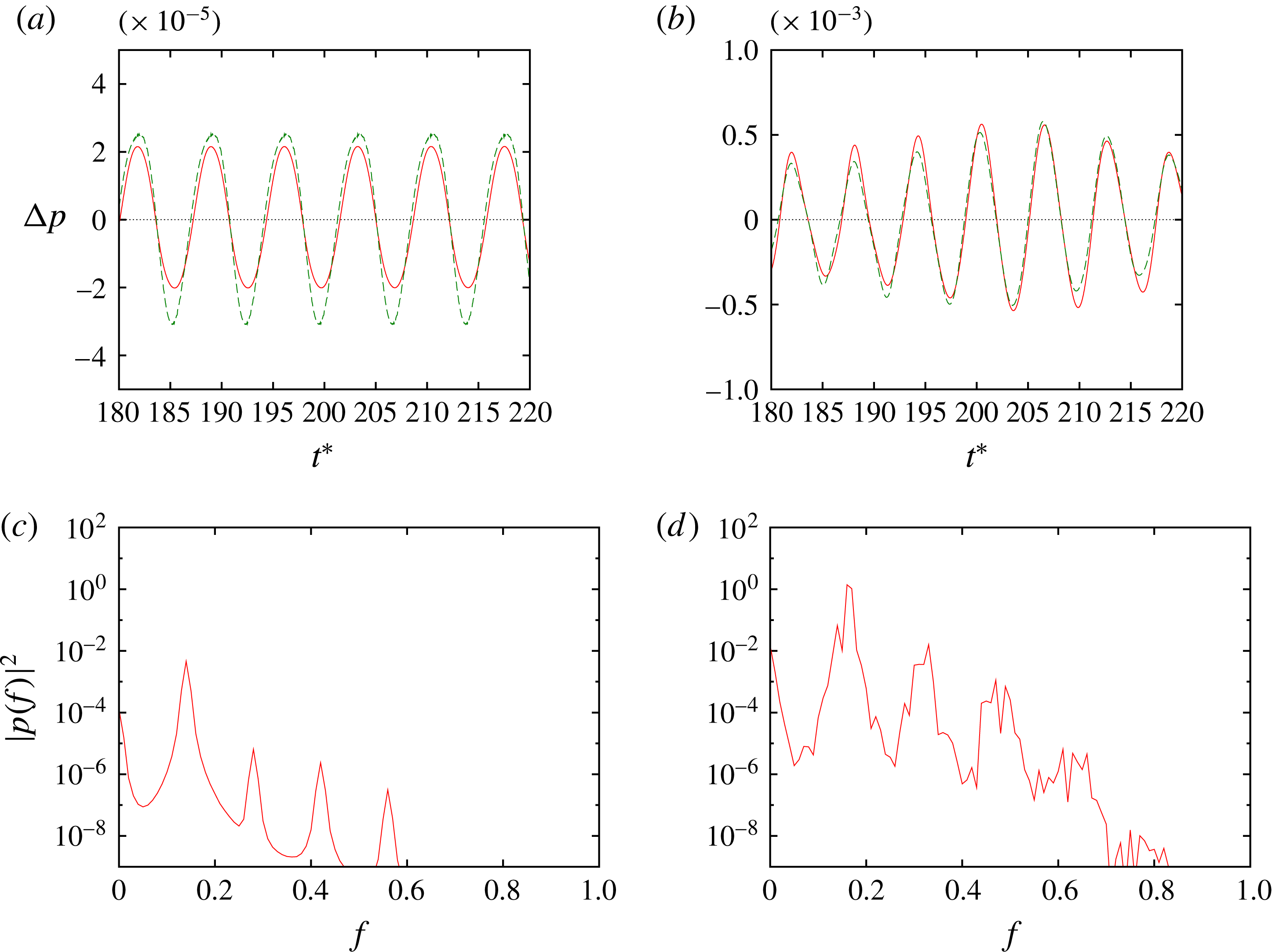
). In the former case the time history of the sound pressure is almost sinusoidal, with the fundamental frequency coinciding with that of the cylinder oscillation; in this case the vortex motion also synchronizes with the cylinder oscillation, although it is not shown here since vorticity field looks quite similar to figure 2(a); it will be shown later when we discuss the phase differences of the forces (figure 13). In the non-periodic case, on the other hand, the time history of the sound pressure is modulated although the cylinder oscillation frequency is equal to the natural frequency; correspondingly, the spectrum of the sound pressure has a rather broad peak at
 $f=St=Sc$
; in this case the vortex motion downstream of the fixed cylinder is not periodic, although the vortex shedding from the oscillating cylinder is periodic.
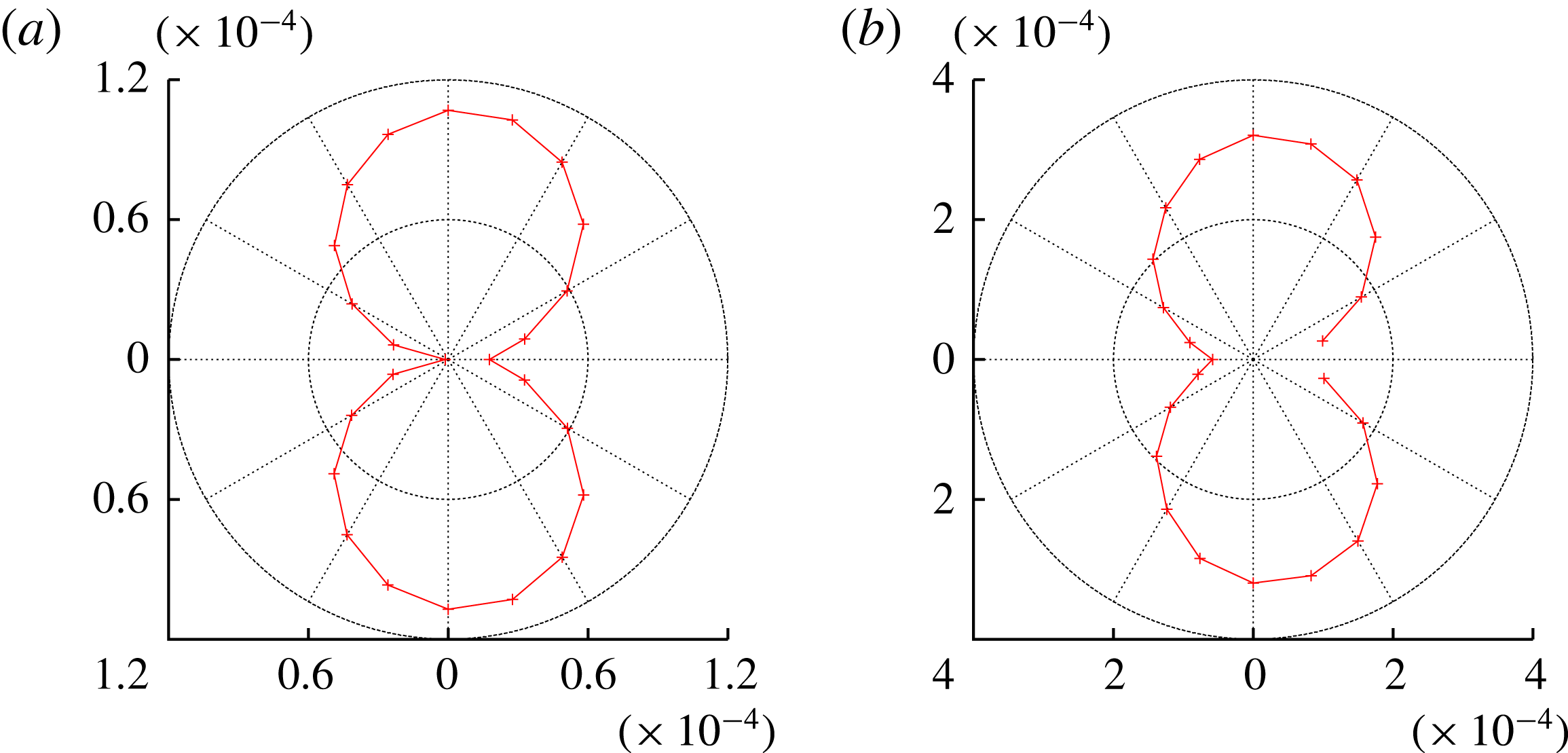
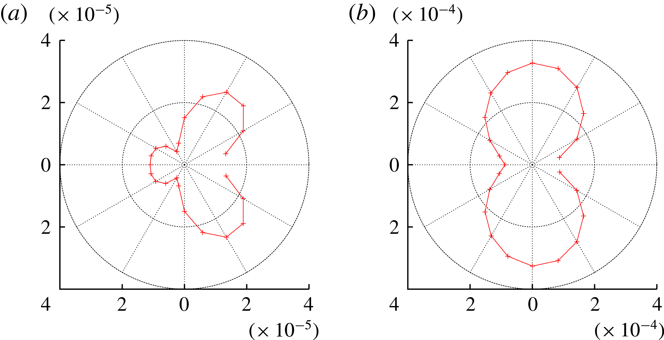
Figure 8 also confirms that the predictions by the Ffowcs Williams–Hawkings equation are in good agreement with the DNS results. The directivity of the sound is nearly dipolar in both cases (figure 9).
(a,b) Time history and (c,d) spectrum of sound pressure at
 $(r/D,\unicode[STIX]{x1D703})=(80,90^{\circ })$
. Oscillating cylinder in front and fixed cylinder behind it. In (a,b) DNS results are shown by the solid lines, while predictions by the Ffowcs Williams–Hawkings equation are shown by dashed lines. (a,c)
 $Sc=0.14$
,
 $L/D=2.0$
, (b,d)
 $Sc=0.18349$
,
 $L/D=4.0$
.

Directivity of sound. Oscillating cylinder in front and fixed cylinder behind it. Polar plot of the r.m.s. amplitude of the sound pressure at
 $r/D=80$
. (a)
 $Sc=0.14$
,
 $L/D=2.0$
, (b)
 $Sc=0.18349$
,
 $L/D=4.0$
.

4.2 Sound reduction and its mechanism
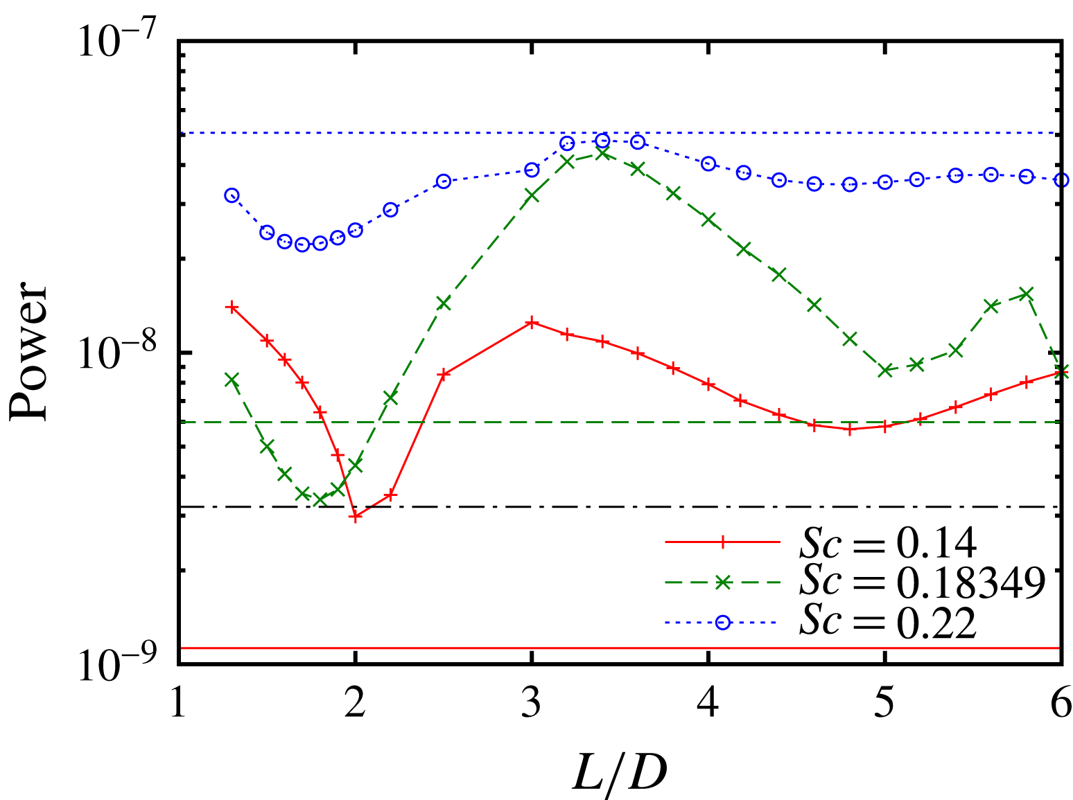
Figure 10 shows the acoustic power, which is calculated in the same way as in the single-oscillating-cylinder case, as a function of the distance between the cylinders. Strong dependence on the distance is observed; for
 $Sc=0.18349$
the minimum is
 $3.38\times 10^{-9}$
at
 $L/D=1.8$
, which is approximately
 $7.8\,\%$
of the maximum
 $4.37\times 10^{-8}$
at
 $L/D=3.4$
; the dependence is relatively weak for
 $Sc=0.22$
, the ratio of the minimum to the maximum being approximately 47 %. There are two local minima for each value of
 $Sc$
, one of which is at
 $L/D\leqslant 2.0$
and the other is at
 $L/D\approx 5.0$
, while the former is sharper than the latter. The minimum at
 $L/D\leqslant 2.0$
shifts to smaller values as
 $Sc$
increases:
 $L/D=2.0$
, 1.8 and 1.7 for
 $Sc=0.14,0.18349$
and 0.22, respectively. The flow is nearly periodic at all values of
 $L/D$
for
 $Sc=0.14$
, while it is not periodic at large values of
 $L/D$
for
 $Sc=0.18349$
and 0.22. Compared to the case of a single oscillating cylinder of the same frequency, the acoustic power is larger than in the single-cylinder case at all values of
 $L/D$
for
 $Sc=0.14$
; it is smaller than in the single-cylinder case near the minimum at
 $L/D=1.8$
for
 $Sc=0.18349$
; for
 $Sc=0.22$
it is smaller than in the single-cylinder case at all values of
 $L/D$
. These results will be discussed in the final section from the viewpoint of sound reduction.
Acoustic power as a function of distance between the two cylinders. Oscillating cylinder in front and fixed cylinder behind it. Solid line and
 $+$
,
 $Sc=0.14$
; dashed line and
 $\times$
,
 $Sc=0.18349$
; dotted line and ○,
 $Sc=0.22$
. The horizontal lines show the acoustic power for a single cylinder: solid line,
 $Sc=0.14$
; dashed line,
 $Sc=0.18349$
; dotted line,
 $Sc=0.22$
; dot-dashed line, fixed cylinder (
 $A/D=0$
).

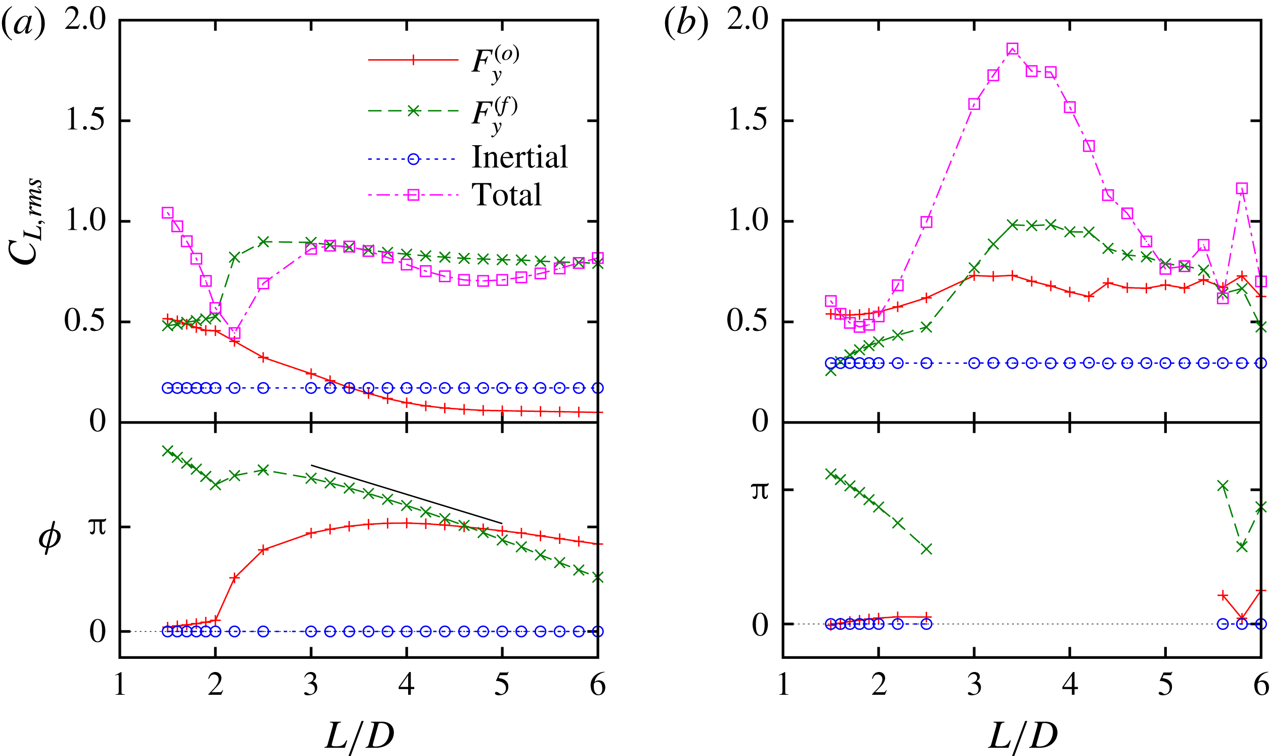
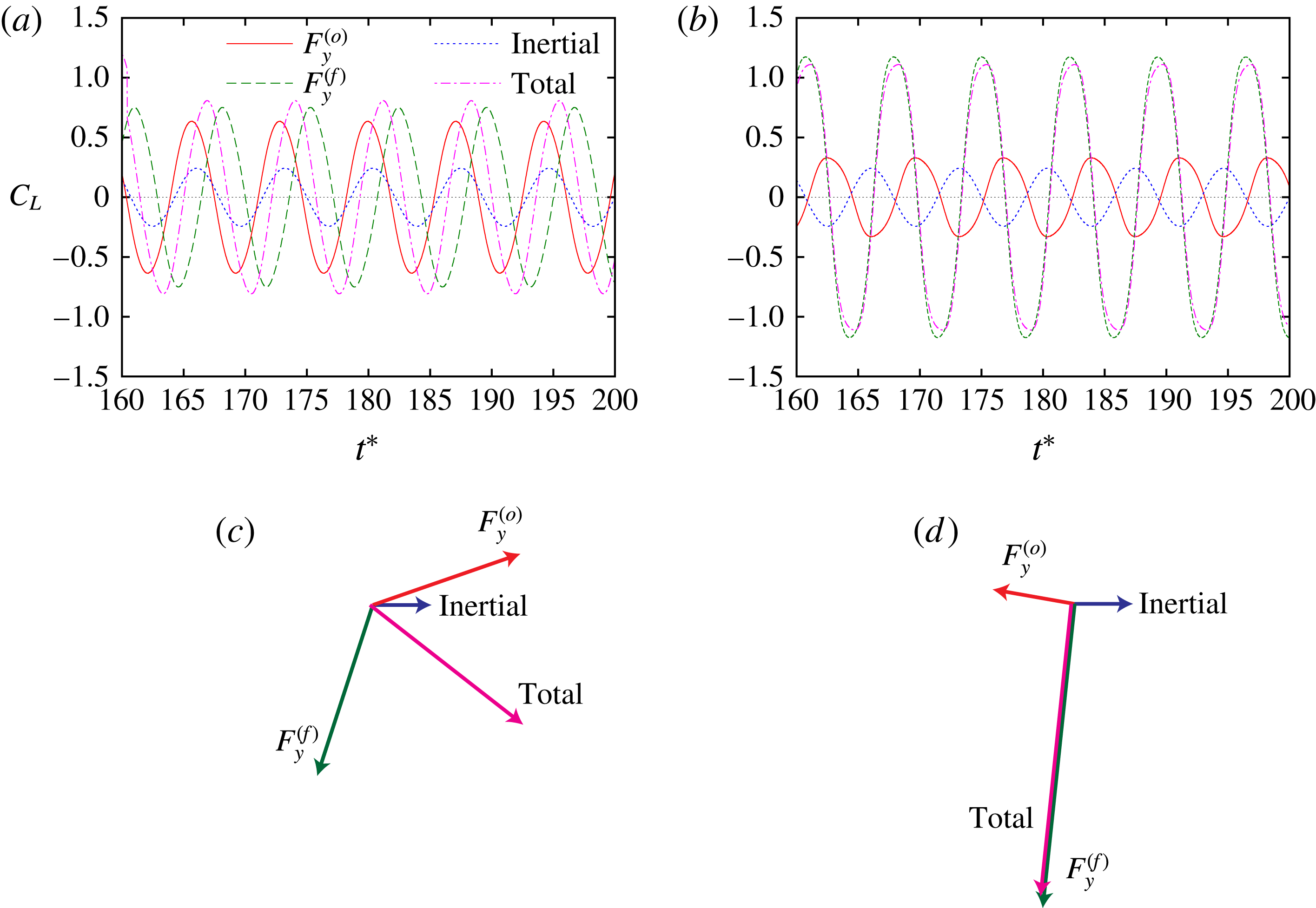
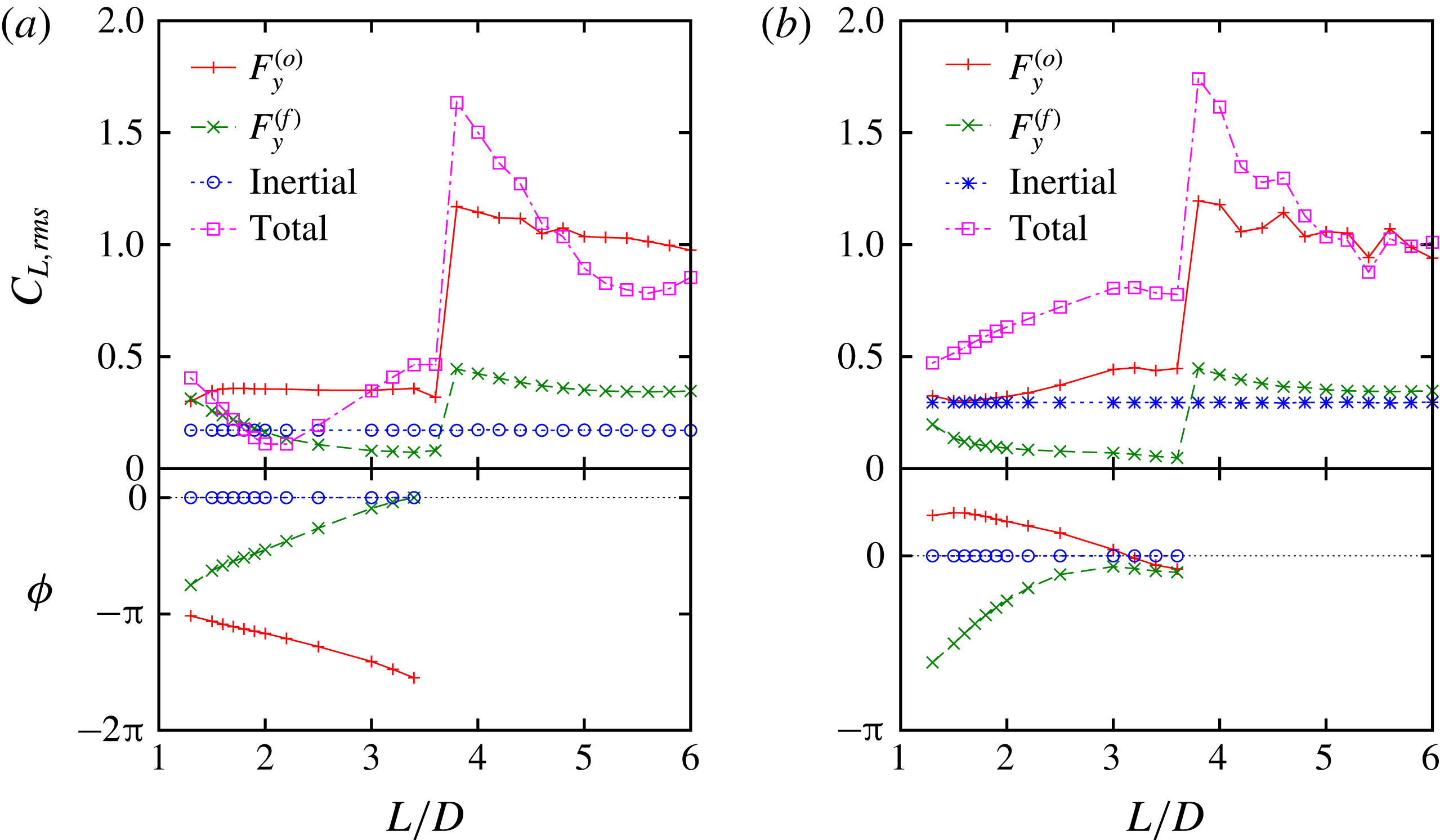
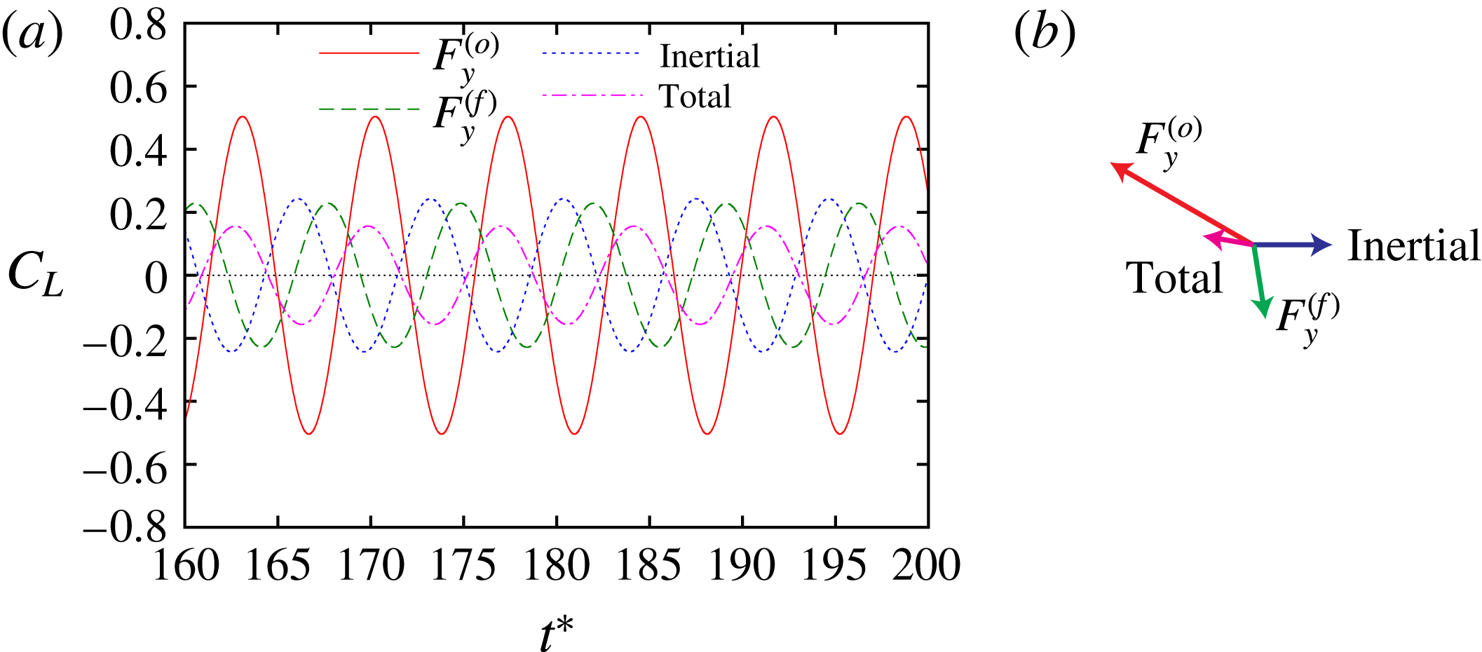
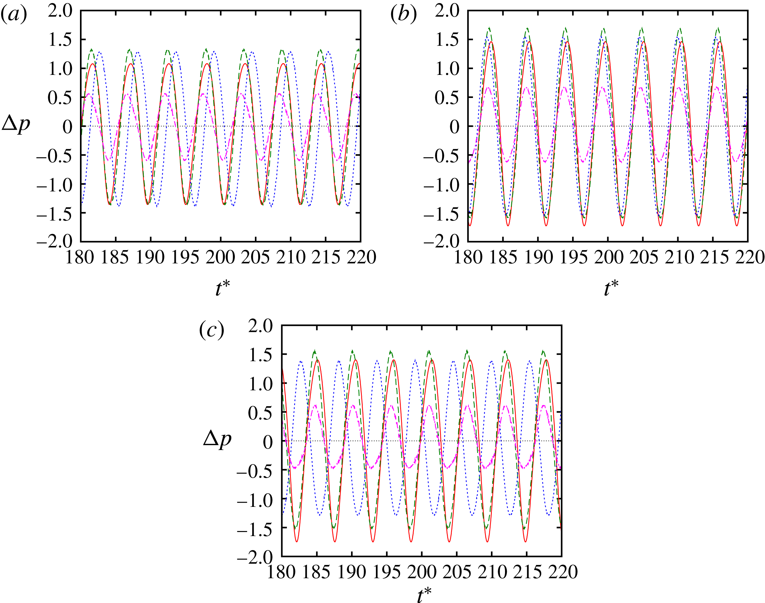
The dependence of the acoustic power on the distance between the cylinders is again understood in terms of the Ffowcs Williams–Hawkings equation, since that gives good predictions of the DNS results. Figure 11 shows the characteristics of the three forces that are required in the Ffowcs Williams–Hawkings equation: the lift forces exerted on the oscillating and the fixed cylinders and the inertial force due to the volume displacement effect. Here the top panel shows the magnitudes of the forces, while the bottom panel shows the phases of the forces, which are defined in the same way as in the single-oscillating-cylinder case with the phase of the inertial force being set to zero. They are well defined only when the forces are nearly periodic as in figure 12.
For
 $Sc=0.14$
the flow can be classified into three regimes. (i) For
 $L/D\leqslant 2.0$
the two cylinders are so close that they may be regarded as a deforming single obstacle (figure 13); the magnitudes of the lift forces exerted on the two cylinders are approximately equal and are much larger than the inertial force. (ii) For
 $2.0\leqslant L/D\lesssim 4.0$
the distance is long enough to allow vortex shedding from the oscillating cylinder but is still short in the sense that interaction between the two cylinders through fluid motion are strong. The lift force
 $F_{y}^{(o)}$
exerted on the oscillating cylinder decays monotonically with
 $L/D$
; on the other hand,
 $F_{y}^{(f)}$
increases for
 $2.0\leqslant L/D\leqslant 2.5$
and then does not vary much with
 $C_{L,rms}=0.8{-}0.95$
for
 $L/D\geqslant 2.5$
. (iii) For
 $L/D\gtrsim 4.0$
the lift coefficient of
 $F_{y}^{(o)}$
is less than 0.1 and converges to the value 0.05 for the single oscillating cylinder as
 $L/D$
increases (figure 11
a). In this case the distance is so large that the existence of the fixed cylinder downstream is expected not to affect the flow near the oscillating cylinder and the resulting force very much. If we assume that the vortices shed from the oscillating cylinder move with the uniform flow velocity
 $U$
, the time required to reach the fixed cylinder from the oscillating cylinder is
 $L/U$
. Then the phase of
 $F^{(f)}$
at large
 $L/D$
is expected to decrease linearly as
 $$\begin{eqnarray}\displaystyle \unicode[STIX]{x1D719}=-2\unicode[STIX]{x03C0}\frac{L/U}{D/(ScU)}=-2\unicode[STIX]{x03C0}Sc\frac{L}{D}, & & \displaystyle\end{eqnarray}$$
the slope of which is shown by the solid line in figure 11(a).
Magnitude and phase of forces in
 $y$
direction: (a)
 $Sc=0.14$
; (b)
 $Sc=0.18349$
. Oscillating cylinder in front and fixed cylinder behind it. The magnitudes and phases are the same as in the case of a single oscillating cylinder, while the phase of the inertial force is chosen to be zero. Solid line and
 $+$
, the lift force exerted on the oscillating cylinder
 $F_{y}^{(o)}$
; dashed line and
 $\times$
, the lift force exerted on the fixed cylinder
 $F_{y}^{(f)}$
; dotted line and ○, the inertial force due to volume displacement effect; dot-dashed line and ▫, the total force.

(a,b) Time history and (c,d) complex amplitude of force: (a,c)
 $L/D=2.0$
; (b,d)
 $L/D=3.0$
. Oscillating cylinder in front and fixed cylinder behind it with
 $Sc=0.14$
. In (a,b) the solid, dashed, dotted and dot-dashed lines show the lift force exerted on the oscillating cylinder
 $F_{y}^{(o)}$
, the lift force exerted on the fixed cylinder
 $F_{y}^{(f)}$
, the inertial force due to volume displacement effect and the total force, respectively. In (c,d) the complex amplitudes of the Fourier mode at
 $f=Sc$
are shown as vectors in the complex plane.

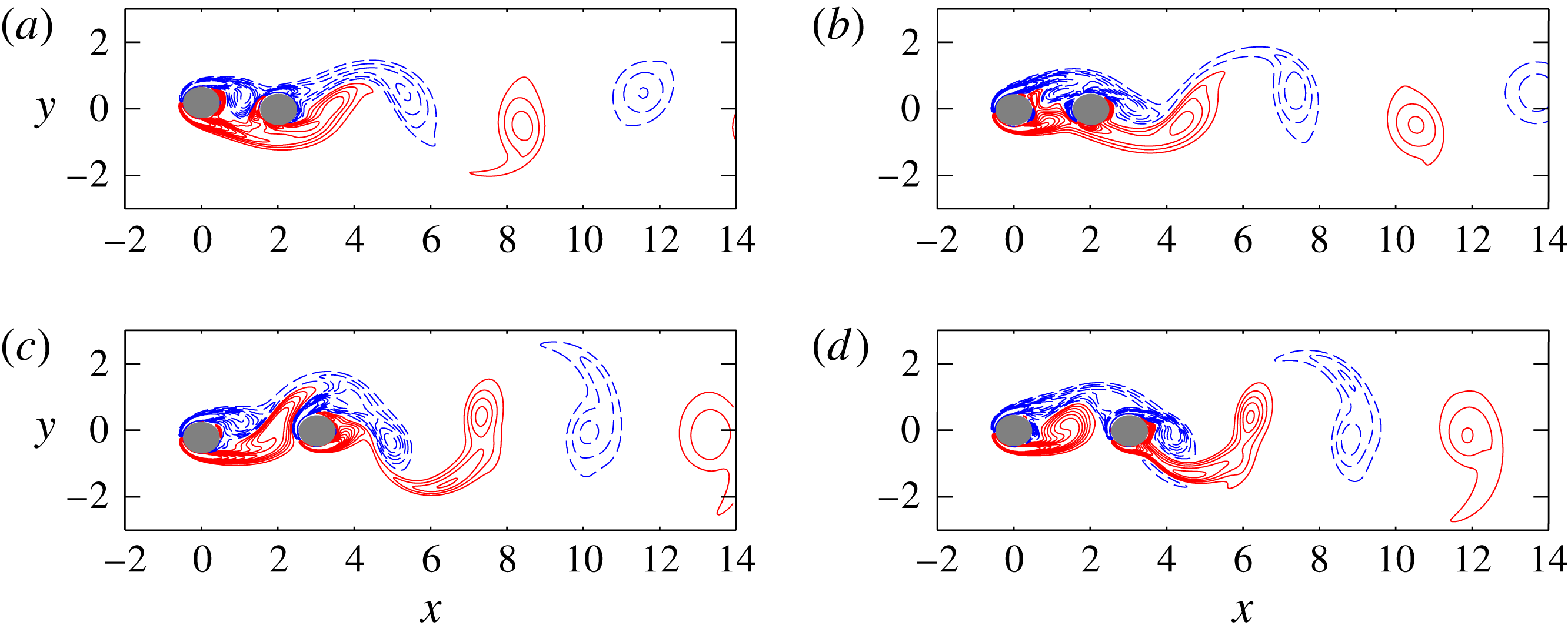
Vorticity field. Oscillating cylinder in front and fixed cylinder behind it. Solid and dashed lines show positive and negative values, respectively. Here
 $Sc=0.14$
; (a)
 $L/D=2.0$
,
 $t^{\ast }=180$
(
 $F_{y}^{(o)}$
is maximum); (b)
 $L/D=2.0$
,
 $t^{\ast }=182.4$
(
 $F_{y}^{(f)}$
is maximum); (c)
 $L/D=3.0$
,
 $t^{\ast }=183.8$
(
 $F_{y}^{(o)}$
is maximum); (d)
 $L/D=3.0$
,
 $t^{\ast }=182.2$
(
 $F_{y}^{(f)}$
is maximum).

The local minimum of the total force at
 $L/D=2.2$
, which is close to
 $L/D=2.0$
at which the acoustic power takes a local minimum, is due to the phase difference between the forces exerted on the two cylinders, which is close to
 $\unicode[STIX]{x03C0}$
and compensates the increase of the force on the fixed cylinder. On the other hand, the local minimum at
 $L/D=4.8$
is caused by the phase difference between
 $F_{y}^{(f)}$
and the inertial force, which crosses
 $\unicode[STIX]{x03C0}$
at
 $L/D=4.8$
, with
 $F_{y}^{(o)}$
being negligible. Figure 12 confirms how the phase differences between the forces determine the total force: at
 $L/D=2.0$
the phase difference between
 $F_{y}^{(o)}$
and
 $F_{y}^{(f)}$
is
 $0.703\unicode[STIX]{x03C0}$
, making the total force small; at
 $L/D=3.0$
,
 $F_{y}^{(o)}$
and the inertial force cancel each other, as the phase difference is close to
 $\unicode[STIX]{x03C0}$
and the magnitudes are close, which make the total force nearly identical with
 $F_{y}^{(f)}$
. In figure 13 the vorticity field is shown at maxima of
 $F_{y}^{(o)}$
and
 $F_{y}^{(f)}$
. At the maximum of
 $F_{y}^{(o)}$
a vortex is about to be shed from the upper side of the oscillating cylinder, while it is blocked by the fixed cylinder for
 $L/D=2.0$
; for
 $L/D=3.0$
a part of the vortex shed from the lower side is seen to move to the upper side of the fixed cylinder. At the maximum of
 $F_{y}^{(f)}$
a vortex shed from the oscillating cylinder collides with the fixed cylinder on the upper side from which a vortex is about to be shed; for
 $L/D=3.0$
the vortex shed from the oscillating cylinder merges with the vortex shed from the fixed cylinder to form an elongated vortex.
For
 $Sc=0.18349$
, the phases of the forces are not well defined for
 $3.0\leqslant L/D\leqslant 5.4$
, which makes it difficult to interpret the local minimum of the acoustic power at
 $L/D=4.8$
. However, the local minimum of the total force at
 $L/D=1.8$
is caused by the same mechanism as the minimum at
 $L/D=2.2$
for
 $Sc=0.14$
. In fact, the phase difference between
 $F_{y}^{(o)}$
and
 $F_{y}^{(f)}$
crosses
 $\unicode[STIX]{x03C0}$
at
 $L/D=1.8$
, while the phase of
 $F_{y}^{(o)}$
nearly coincides with that of the inertial force.
5 Flow past fixed and oscillating cylinders
In this section we reverse the positions of the oscillating cylinder and the fixed cylinder; namely, the oscillating cylinder is now located in the wake of the fixed cylinder (figure 1 c). The parameter values are the same as in the previous section.
5.1 Vortex motion and sound propagation
Figure 14 shows time histories of sound pressure at
 $(r/D,\unicode[STIX]{x1D703})=(80,90^{\circ })$
and their power spectra for two particular cases,
 $L/D=2.0$
and 4.0 with
 $Sc=0.14$
. In this case the flow can be classified into two regimes: (i) When the distance between the cylinders is small, the fluid motion locks in to the cylinder oscillation and is periodic, as the fundamental frequency coincides with
 $Sc$
and no peak appears at
 $St$
(figure 14
a,c). In this case the distance between the cylinders is so small that the oscillating cylinder downstream controls the vortex shedding from the fixed cylinder upstream; the two cylinders behave as one deforming obstacle hydrodynamically as in the case of the oscillating cylinder in front with small
 $L/D$
. (ii) When the distance is large, on the other hand, the flow is not periodic and the sound pressure is modulated (figure 14
b); correspondingly, the dominant frequency is the natural frequency
 $St$
, while a small peak is observed at
 $Sc$
(figure 14
d). In this case vortices are shed from the fixed cylinder upstream almost unaffected by the oscillating cylinder, which excites its own frequency weakly.
The prediction by the Ffowcs Williams–Hawkings equation slightly overpredicts the DNS results for
 $L/D=2.0$
(figure 14
a), while it is good for
 $L/D=4.0$
(figure 14
b). For
 $L/D=2.0$
the magnitude of sound pressure is significantly reduced, as shown below, making the relative errors of sound pressure large; note that the range of the sound pressure for
 $L/D=2.0$
is
 $5.0\times 10^{-5}$
, which is 5 % of
 $1.0\times 10^{-3}$
for
 $L/D=4.0$
. As a result the directivity of the sound does not exhibit dipolar nature for
 $L/D=2.0$
(figure 15
a) as the dipolar component due to the drag force and the quadrupolar components are comparable with the reduced dipolar component due to the lift force, which is usually dominant. In contrast, dipolar directivity is observed for
 $L/D=4.0$
(figure 15
b).
(a,b) Time history and (c,d) spectrum of sound pressure at
 $(r/D,\unicode[STIX]{x1D703})=(80,90^{\circ })$
. Fixed cylinder in front and oscillating cylinder behind it. The lines are the same as in figure 8. Here
 $Sc=0.14$
: (a,c)
 $L/D=2.0$
; (b,d)
 $L/D=4.0$
.

Directivity of sound. Fixed cylinder in front and oscillating cylinder behind it. Polar plot of the r.m.s. amplitude of the sound pressure at
 $r/D=80$
. Here
 $Sc=0.14$
: (a)
 $L/D=2.0$
; (b)
 $L/D=4.0$
.

5.2 Sound reduction and its mechanism
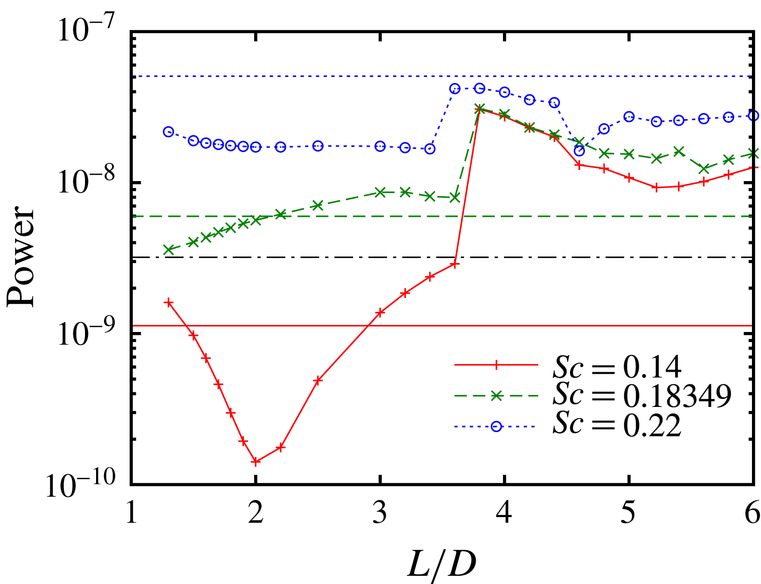
Figure 16 shows the acoustic power as a function of the distance between the cylinders for three values of
 $Sc$
. Significant reduction of the acoustic power is observed around
 $L/D=2.0$
for
 $Sc=0.14$
; the value at
 $L/D=2.0$
is
 $1.41\times 10^{-10}$
, which is
 $0.46\,\%$
of the maximum
 $3.07\times 10^{-8}$
at
 $L/D=3.8$
. However, no clear local minimum is observed in
 $L/D\leqslant 3.0$
for
 $Sc=0.18349$
and
 $2.2$
. The acoustic power jumps up at
 $L/D=3.4{-}3.6$
above which the fluid motion loses synchronization with the cylinder oscillation. There is a shallow local minimum at
 $L/D=5.2$
for
 $Sc=0.14$
as in the case of the oscillating cylinder in front of the fixed cylinder. Compared to the case of the single oscillating cylinder of the same frequency, the acoustic power is significantly reduced from the single-cylinder case near the minimum at
 $L/D=2.0$
for
 $Sc=0.14$
; it is smaller than the single-cylinder case near the minimum at
 $L/D\leqslant 2.0$
for
 $Sc=0.18349$
; for
 $Sc=0.22$
it is smaller than the single-cylinder case at all values of
 $L/D$
as in the case of the oscillating cylinder in front. These results will also be discussed in the final section from the viewpoint of sound reduction.
Acoustic power as a function of distance between cylinders. Fixed cylinder in front and oscillating cylinder behind it. Solid line and
 $+$
,
 $Sc=0.14$
; dashed line and
 $\times$
,
 $Sc=0.18349$
; dotted line and ○,
 $Sc=0.22$
. The horizontal lines show the acoustic power for a single cylinder: solid line,
 $Sc=0.14$
; dashed line,
 $Sc=0.18349$
; dotted line,
 $Sc=0.22$
; dot-dashed line, fixed cylinder (
 $A/D=0$
).

As in the previous section, we seek to understand the mechanism of sound reduction by investigating the forces appearing in the Ffowcs Williams–Hawkings equation. The characteristics of the forces depend on whether the flow is periodic or not. For
 $Sc=0.14$
the flow is periodic when
 $L/D\leqslant 3.4$
and not periodic otherwise. For
 $L/D\leqslant 3.4$
the lift force exerted on the oscillating cylinder is nearly constant, the lift force exerted on the fixed cylinder decays monotonically, and the phases of the forces are well defined (figure 17
a). Then the two forces jump up at
 $L/D=3.8$
above which the flow loses synchronization with the cylinder oscillation. These increases of the forces cause the increase of the acoustic power in figure 16(a).
The significant reduction of sound at
 $L/D=2.0$
for
 $Sc=0.14$
is caused by cancellation of the three forces. The magnitude of the oscillating cylinder force is approximately 2.4 times those of the other two forces; its phase is
 $-1.17\unicode[STIX]{x03C0}$
, while that of the fixed cylinder force is
 $-0.45\unicode[STIX]{x03C0}$
. Thus both the fixed cylinder force and the inertial force contribute to reduce the total force (figure 18
b). As a result the magnitude of the total force is smaller than those of the three forces as shown in figure 18(a). In figure 19(a,b) a vortex is about to be shed from the upper/lower side of the fixed cylinder upstream, while another vortex is being shed from the lower/upper side of the oscillating cylinder downstream, which is consistent with nearly antiphase time dependence of
 $F_{y}^{(f)}$
and
 $F_{y}^{(o)}$
.
For
 $Sc=0.18349$
the magnitudes of the forces vary in a similar way as for
 $Sc=0.14$
, but the phase of the oscillating cylinder force is different from that for
 $Sc=0.14$
. As a result no significant reduction of the acoustic power occurs.
Magnitude and phase of forces in
 $y$
direction: (a)
 $Sc=0.14$
; (b)
 $Sc=0.18349$
. Fixed cylinder in front and oscillating cylinder behind it. The lines and symbols are the same as in figure 11.

(a) Time history and (b) complex amplitude of force. Fixed cylinder in front and oscillating cylinder behind it. Here
 $Sc=0.14$
,
 $L/D=2.0$
. The lines and symbols are the same as in figure 12.

Vorticity field. Fixed cylinder in front and oscillating cylinder behind it. Solid and dashed lines show positive and negative values, respectively. Here
 $Sc=0.14$
,
 $L/D=2.0$
: (a)
 $t^{\ast }=182$
(
 $F_{y}^{(f)}$
is maximum); (b)
 $t^{\ast }=184.6$
(
 $F_{y}^{(o)}$
is maximum).

Acoustic power reduction by adding a cylinder;
 $A/D=0.2$
. In this table
 $P_{s}$
is the acoustic power in the single-oscillating-cylinder case, while
 $P_{f}=3.203\times 10^{-9}$
is for the fixed cylinder; both
 $P_{s}$
and
 $P_{f}$
are taken as the reference values for discussion of sound reduction;
 $P_{min}$
denotes the minimum acoustic power in figures 10 (oscillating in front) and 16 (fixed in front) at each
 $Sc$
.

6 Concluding remarks
We have studied the sound generation in a two-dimensional low-Reynolds-number flow past (i) a single oscillating cylinder, (ii) an oscillating cylinder in front and a fixed cylinder behind it and (iii) a fixed cylinder in front and an oscillating cylinder behind it. The aeroacoustic sound was successfully resolved by DNS using the corrected VP method (Komatsu et al.
Reference Komatsu, Iwakami and Hattori2016). The sound pressure was shown to be in good agreement with the prediction by the Ffowcs Williams–Hawkings equation, which takes account of the cylinder motion. For the single oscillating cylinder, the fluid motion can be either periodic or non-periodic depending on the frequency and the amplitude of cylinder oscillation. The acoustic power is significantly reduced when the fluid motion locks in to a frequency lower than the natural frequency of vortex shedding from a fixed cylinder. When a fixed cylinder is added, the acoustic power depends strongly on the distance between the cylinders. Two local minima of the acoustic power were observed when the fixed cylinder is placed in the wake of the oscillating cylinder. One is a sharp minimum at
 $L/D=1.7{-}2.0$
depending on the frequency of cylinder oscillation; in terms of the Ffowcs Williams–Hawkings equation it is caused by the phase difference between the lift forces exerted on the two cylinders. The other, which is not so sharp, is caused by the phase difference between the force exerted on the fixed cylinder and the inertial force due to the volume displacement effect. When the fixed cylinder is placed in front of the oscillating cylinder, the fluid motion is periodic with the frequency of cylinder oscillation for small distance between the cylinders, as the two cylinders behave as one deforming obstacle aerodynamically. Significant sound reduction is observed at
 $L/D=2.0$
for
 $Sc=0.14$
; in this case, three forces cooperate to reduce the acoustic power. For large distance, however, the fluid motion is non-periodic and the acoustic power becomes large.
It should be pointed out that the acoustic power depends strongly on synchronization and phase difference of the forces, both of which can be controlled by the positions and motion of the cylinders. In this regard the present results also show that sound reduction by adding obstacles is possible. In fact, aeroacoustic sound generated in flow past a single oscillating cylinder can be reduced by placing a fixed cylinder; aeroacoustic sound generated in flow past a fixed cylinder can be reduced by placing an oscillating cylinder. Table 1 shows when and how much acoustic power is reduced. In this table,
 $P_{s}$
is the acoustic power in the single-oscillating-cylinder case;
 $P_{s}$
is the reference value of the acoustic power when we consider sound reduction in flow past a single oscillating cylinder by placing a fixed cylinder;
 $P_{f}$
is the acoustic power in the fixed-cylinder case;
 $P_{f}$
is the reference value of the acoustic power when we consider sound reduction in flow past a fixed cylinder by placing an oscillating cylinder;
 $P_{min}$
denotes the minimum acoustic power in figures 10 (oscillating in front) and 16 (fixed in front) at each
 $Sc$
. In particular, for
 $Sc=0.14$
the acoustic power of the single oscillating cylinder is reduced to 12.5 % by placing a fixed cylinder in front, while that of the fixed cylinder is reduced to 4.4 % by placing an oscillating cylinder in its wake. Of course, these effects depend significantly on parameters like frequency, amplitude and distance between the cylinders; the Reynolds number is too low for practical applications. Nevertheless, it should be emphasized that the present results have shown the possibility and essential mechanism of sound reduction by adding obstacles. Even in high-Reynolds-number flows there often exists a dominant frequency of fluid motion and sound; then the present results can give a clue to control and reduce aeroacoustic noise.
Another important achievement of the present paper is that the corrected VP method is shown to be useful for DNS of aeroacoustic sound in time-varying geometry as good agreement with the Ffowcs Williams–Hawking acoustic analogy is confirmed. It is also pointed out that DNS is reliable when the sound is significantly reduced, although the Ffowcs Williams–Hawking acoustic analogy, which does not include the quadrupolar or higher contributions, fails to give a good prediction. It can be applied to various problems in which rigid bodies move with different speeds and/or deformable bodies are involved.
Acknowledgements
This work was supported by Kawai Foundation for Sound Technology and Music. Numerical calculations were performed on the UV1000 and UV2000 at the Institute of Fluid Science, Tohoku University.
Appendix A. Accuracy of the corrected VP method in the acoustic scattering from two cylinders
Although the accuracy of the corrected VP method has been established for aeroacoustic problems in Komatsu et al. (Reference Komatsu, Iwakami and Hattori2016), it has not been checked in the scattering of high-frequency acoustic waves from rigid bodies. In this appendix, we check it for acoustic scattering from two cylinders, which is one of the standard benchmark problems in computational aeroacoustics (Dahl Reference Dahl2004; Sherer Reference Sherer2004) and considered in assessment of linear acoustic simulations using the immersed boundary method (Seo & Mittal Reference Seo and Mittal2011; Bae & Moon Reference Bae and Moon2012).
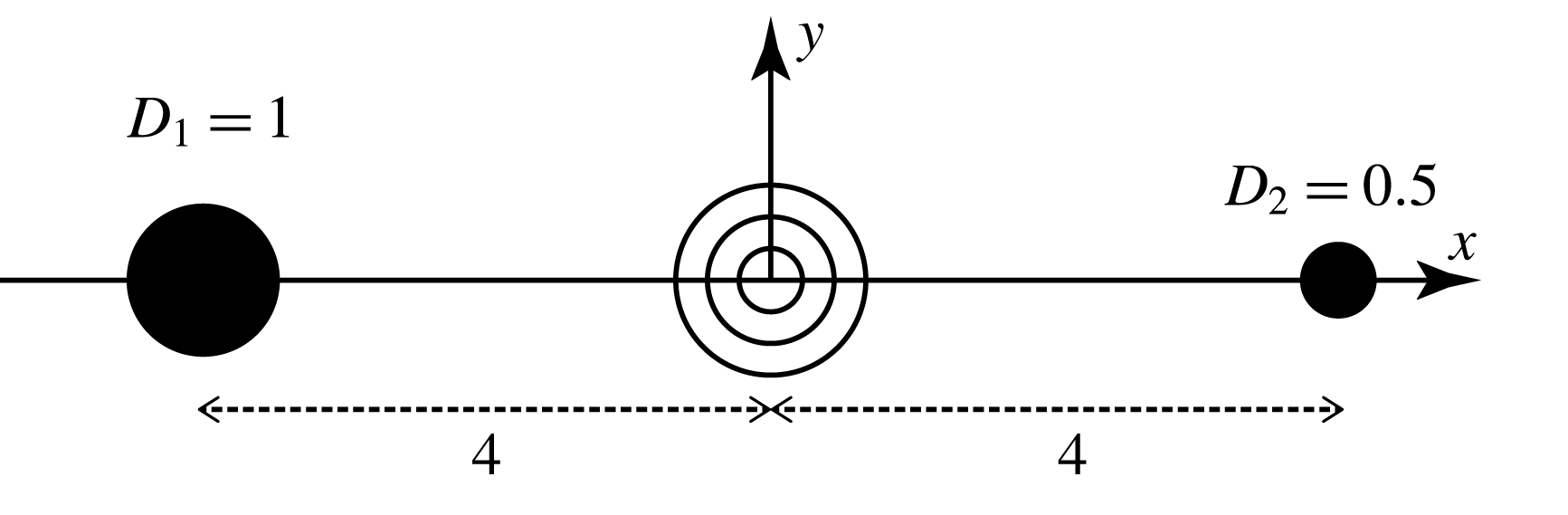
Acoustic scattering from two cylinders. Schematic diagram.

The schematic diagram of the problem is shown in figure 20. Two cylinders of unequal diameters (
 $D_{1}=1$
and
 $D_{2}=0.5$
) are located at
 $x=\pm 4$
. A sound source is located at the origin; the following source term
 $S$
is added to the right-hand side of (2.3),
 $$\begin{eqnarray}\displaystyle S=\frac{A}{\unicode[STIX]{x1D6FE}-1}\exp \left[-\frac{\log 2}{b^{2}}(x^{2}+y^{2})\right]\sin \unicode[STIX]{x1D714}t, & & \displaystyle\end{eqnarray}$$
where
 $b=0.2$
and
 $\unicode[STIX]{x1D714}=8\unicode[STIX]{x03C0}$
as in Dahl (Reference Dahl2004). The amplitude is set small at
 $A=10^{-4}$
to assure that acoustic waves are nearly linear.
Equations (2.1)–(2.3) are solved numerically by the same methods as described in § 2.2. To check the dependence on the penalization parameters, the porosity
 $\unicode[STIX]{x1D719}$
is chosen from
 $\{0.1,0.3,1\}$
and the permeability
 $\unicode[STIX]{x1D702}=\unicode[STIX]{x1D702}_{T}$
is chosen from
 $\{10^{-6},10^{-5},10^{-4},10^{-3}\}$
. In most cases considered in this appendix, the grid size is nearly constant,
 $\unicode[STIX]{x0394}x=\unicode[STIX]{x0394}y=0.01$
, in a rectangular domain
 $|x|\leqslant 9$
,
 $|y|\leqslant 5$
, while it is gradually stretched outside it. Larger values of the grid size are also used to check grid convergence:
 $\unicode[STIX]{x0394}x=\unicode[STIX]{x0394}y=0.014$
, 0.02 and 0.028.
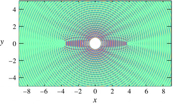
Acoustic scattering from two cylinders. Snapshot of sound pressure.

Figure 21 shows a snapshot of the pressure field obtained by DNS with
 $\unicode[STIX]{x1D719}=0.1$
and
 $\unicode[STIX]{x1D702}=10^{-5}$
. Acoustic waves of wavelength
 $\unicode[STIX]{x1D706}=0.25$
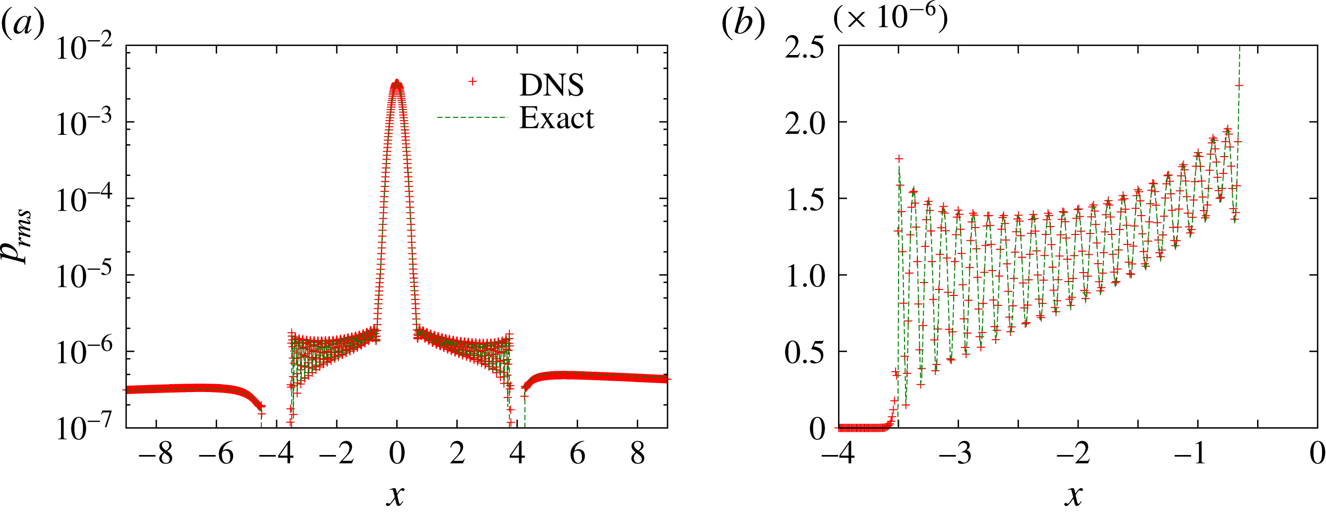
are radiated from the source and scattered from the cylinders. This figure is similar to those obtained in the previous works (Seo & Mittal Reference Seo and Mittal2011; Bae & Moon Reference Bae and Moon2012). Figure 22 compares the r.m.s. amplitude of pressure between the exact solution and DNS. They are in good agreement.
Acoustic scattering from two cylinders. Comparison of the r.m.s. amplitude of pressure along
 $y=0$
for: (a)
 $-9\leqslant x\leqslant 9$
; (b)
 $4\leqslant x\leqslant 0$
. Here
 $\unicode[STIX]{x1D719}=0.1$
,
 $\unicode[STIX]{x1D702}=10^{-5}$
; symbols, DNS; dashed line, exact solution.

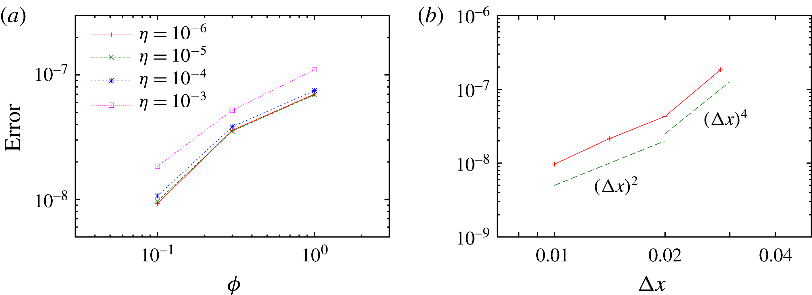
Figure 23 shows that the error becomes small for appropriate choice of parameters. Here the error is defined as the average of the difference between the local extrema of the r.m.s. amplitude of pressure along
 $y=0,~0.5<|y|<3.5$
,
 $$\begin{eqnarray}\displaystyle \text{error}=\frac{1}{N_{ex}}\mathop{\sum }_{i}|p_{ex,i}^{(DNS)}-p_{ex,i}^{(exact)}|, & & \displaystyle\end{eqnarray}$$
where
 $N_{ex}$
is the number of extrema (both maxima and minima), and
 $p_{ex,i}^{(DNS)}$
and
 $p_{ex,i}^{(exact)}$
are the
 $i$
th extremum (local maximum or minimum) of the r.m.s. amplitude of DNS data and the exact solution, respectively. The error decreases as
 $\unicode[STIX]{x1D719}$
and
 $\unicode[STIX]{x1D702}$
decrease; the relative error is 0.82 % for
 $\unicode[STIX]{x1D719}=0.1$
and
 $\unicode[STIX]{x1D702}=10^{-5}$
. Compared to the aeroacoustic case (Komatsu et al.
Reference Komatsu, Iwakami and Hattori2016),
 $\unicode[STIX]{x1D719}$
should be chosen smaller in the present case; the error is sufficiently small only for
 $\unicode[STIX]{x1D719}=0.1$
and
 $\unicode[STIX]{x1D702}\leqslant 10^{-4}$
, although all values of
 $\unicode[STIX]{x1D719}$
give satisfactory results for
 $\unicode[STIX]{x1D702}\leqslant 10^{-3}$
in the sound generation in flow past a fixed cylinder. This difference comes from the frequency of the acoustic waves. In order to capture reflection of high-frequency acoustic waves, the penalization parameters should be chosen sufficiently small, as suggested by the analytical results by Liu & Vasilyev (Reference Liu and Vasilyev2007).
The grid convergence is also checked in figure 23(b), which shows that the error decreases with the grid size. There are three major sources of error in the present case: (i) spatial discretization, (ii) ambiguity of the surface of the cylinders (or thickness of the surface) and (iii) finite values of penalization parameters (the porosity
 $\unicode[STIX]{x1D719}$
and the permeability
 $\unicode[STIX]{x1D702}$
). For
 $0.02\leqslant \unicode[STIX]{x0394}x\leqslant 0.028$
, the error due to spatial discretization is large and the error is roughly proportional to
 $(\unicode[STIX]{x0394}x)^{4}$
; there are only two data points, however, which makes this dependence somewhat unconvincing. For
 $0.01\leqslant \unicode[STIX]{x0394}x\leqslant 0.02$
, the error is proportional to
 $(\unicode[STIX]{x0394}x)^{2}$
, which is most likely due to the ambiguity of the surface of the cylinders. The surface of the cylinders is only approximately realized with
 $O(\unicode[STIX]{x0394}x)$
error in the VP method since the mask function is defined on a rectangular grid system and the surface does not coincide with grid points in general; thus some amount of errors are caused by this ambiguity. Nevertheless, it is shown that the error decreases with the grid size.
To conclude, the corrected VP method is shown to be sufficiently accurate with appropriate choice of parameters in the problem of high-frequency acoustic scattering.
Acoustic scattering from two cylinders. (a) Errors plotted against the porosity
 $\unicode[STIX]{x1D719}$
, with the permeability
 $\unicode[STIX]{x1D702}=10^{-6}$
,
 $10^{-5}$
,
 $10^{-4}$
and
 $10^{-3}$
. (b) Errors plotted against the grid size, with
 $\unicode[STIX]{x1D719}$
and
 $\unicode[STIX]{x1D702}$
being fixed to 0.1 and
 $10^{-5}$
, respectively.

Appendix B. No-slip boundary conditions at the surface of the moving cylinder
In this appendix we briefly show that no-slip boundary conditions are automatically satisfied at the surface of the moving cylinder by the corrected VP method. The no-slip boundary conditions at the surface of the cylinder are
 $\boldsymbol{u}=\boldsymbol{U}_{0}$
, or, equivalently,
 $$\begin{eqnarray}\displaystyle (\boldsymbol{u}-\boldsymbol{U}_{0})\boldsymbol{\cdot }\boldsymbol{n}=0,\quad (\boldsymbol{u}-\boldsymbol{U}_{0})\boldsymbol{\cdot }\boldsymbol{t}=0, & & \displaystyle\end{eqnarray}$$
where
 $\boldsymbol{n}$
and
 $\boldsymbol{t}$
is the normal and tangential vectors at the surface of the cylinder.
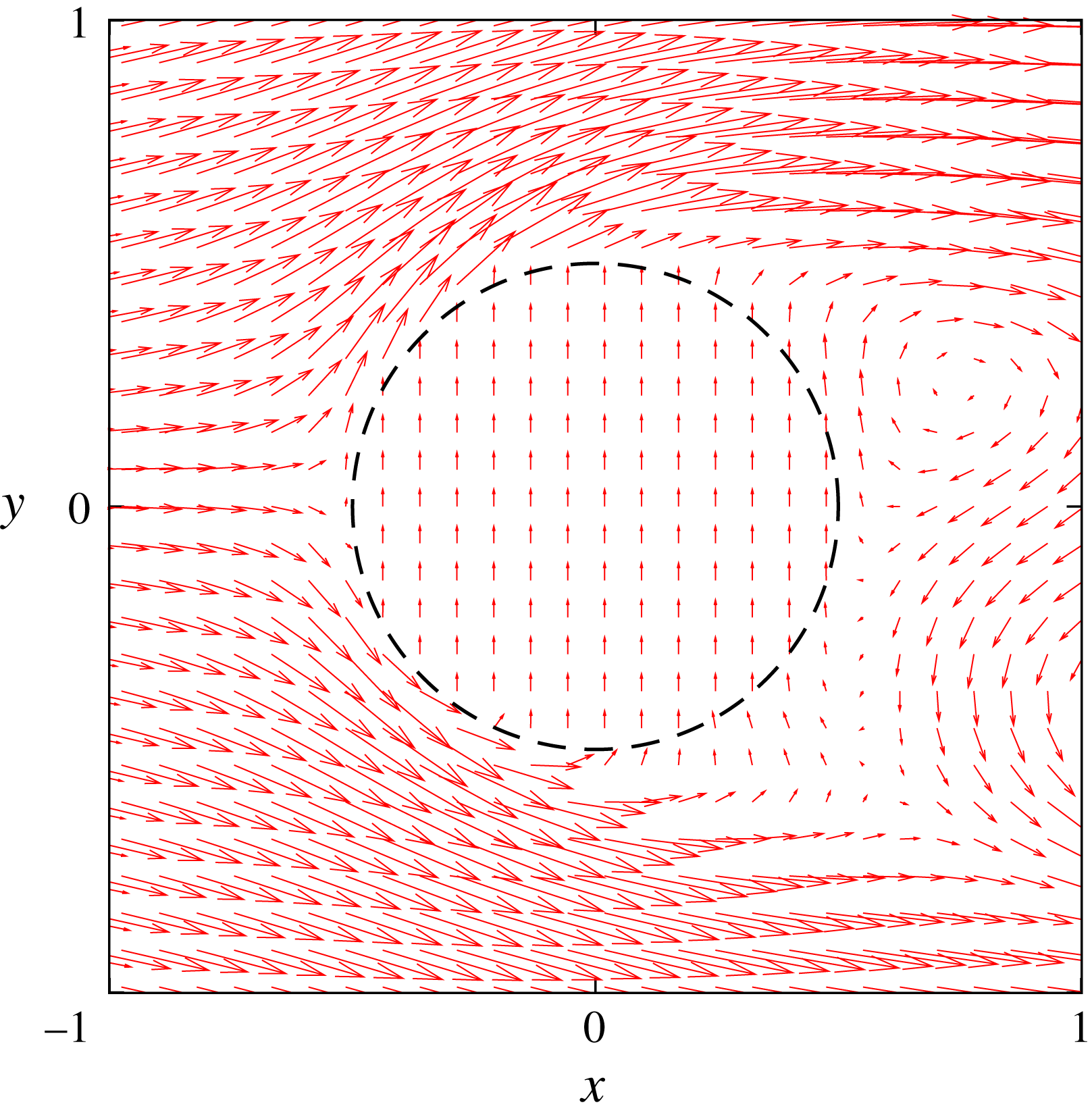
Figure 24 shows the velocity field near the oscillating cylinder at
 $t^{\ast }=178.6$
, when the velocity of the cylinder is nearly maximum. Note that the velocity vectors are shown at every eighth grid lines in the
 $x$
and
 $y$
directions so that the vectors are clearly visible. This figure shows that the velocity inside the cylinder is uniform in the positive
 $y$
direction at
 $t^{\ast }=178.6$
coinciding with the velocity of the cylinder motion.
Velocity field near the oscillating cylinder. Oscillating cylinder in front and fixed cylinder behind it. The dashed line shows the surface of the oscillating cylinder. Here
 $Sc=0.14$
,
 $L/D=2.0$
and
 $t^{\ast }=178.6$
.

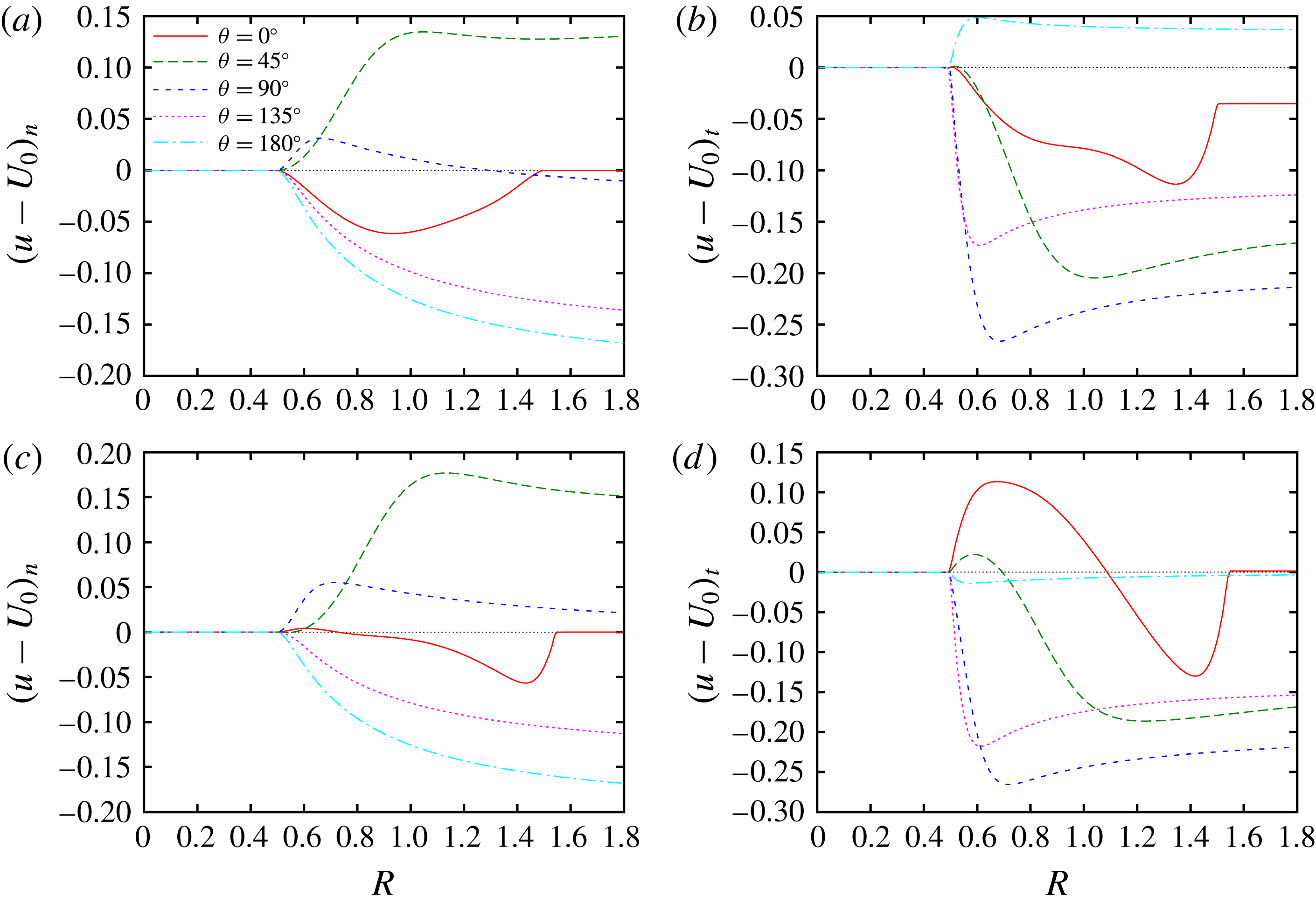
Figure 25 checks the boundary conditions (B 1) for the oscillating cylinder in front and fixed cylinder behind it with
 $Sc=0.14$
and
 $L/D=2.0$
at
 $t^{\ast }=178.6$
and 180.4. The values of the left-hand side of (B 1) are plotted against
 $R$
, which is the distance from the centre of the cylinder for several directions
 $\unicode[STIX]{x1D6E9}$
, which is the angle from the
 $x$
direction. It is evident that the no-slip boundary conditions (B 1) are satisfied as
 $(\boldsymbol{u}-\boldsymbol{U}_{0})\boldsymbol{\cdot }\boldsymbol{n}$
and
 $(\boldsymbol{u}-\boldsymbol{U}_{0})\boldsymbol{\cdot }\boldsymbol{t}$
always vanish for
 $R\leqslant 0.5$
, which corresponds to the inside and surface of the oscillating cylinder.
Distribution of relative velocity
 $\boldsymbol{u}-\boldsymbol{U}_{0}$
. Oscillating cylinder in front and fixed cylinder behind it. Here
 $Sc=0.14$
,
 $L/D=2.0$
and
 $\unicode[STIX]{x1D703}=0^{\circ }$
,
 $45^{\circ }$
,
 $90^{\circ }$
,
 $135^{\circ }$
,
 $180^{\circ }$
: (a,c) the normal components
 $(\boldsymbol{u}-\boldsymbol{U}_{0})\boldsymbol{\cdot }\boldsymbol{n}$
; (b,d) the tangential components
 $(\boldsymbol{u}-\boldsymbol{U}_{0})\boldsymbol{\cdot }\boldsymbol{t}$
; (a,b)
 $t^{\ast }=178.6$
; (c,d)
 $t^{\ast }=180.4$
.

Appendix C. Prediction of sound pressure using the Ffowcs Williams–Hawkings equation
In this appendix we clarify which factors are important in the Ffowcs Williams–Hawkings equation (2.7) to predict the sound pressure correctly. We recall that we have assumed that the sound source is compact, as the flow Mach number is small. In addition the motion of the oscillating cylinder is neglected in evaluating the retarded time; it is not impossible to take account of this motion by solving a nonlinear equation iteratively, but it has little effect on the results since the amplitude of the oscillation is much smaller than the distance between the cylinders and the observation points:
 $A/D=0.2$
,
 $0.5\ll r_{0}/D=80$
.
Time history of sound pressure. Comparison to Ffowcs Williams–Hawkings equation. Oscillating cylinder in front and fixed cylinder behind it. Solid line, DNS; dashed line, the Ffowcs Williams–Hawkings equation (2.7); dotted line, (2.7) without the Doppler effect; dot-dashed line, (2.7) without the inertial force. Here
 $Sc=0.18349$
,
 $L/D=1.8$
,
 $r/D=80$
and
 $\unicode[STIX]{x1D703}=60^{\circ }$
(a),
 $90^{\circ }$
(b) and
 $120^{\circ }$
(c).

In figure 26 the time histories of sound pressure obtained by DNS are compared to predictions based on the Ffowcs Williams–Hawkings equation with different levels of approximations: (i) equation (2.7) is used without further approximation; (ii) the Doppler effect is disregarded, with the Doppler factor
 $C^{(\unicode[STIX]{x1D6FC})}$
being set to
 $1$
; and (iii) the inertial force
 $-\unicode[STIX]{x1D70C}_{0}S_{0}A_{i}^{(\unicode[STIX]{x1D6FC})}$
is ignored. It is evident that both the Doppler effect and the inertial force should be taken into account in order to predict the sound correctly. When the Doppler effect is disregarded, the prediction naturally fails to give the correct phase for
 $\unicode[STIX]{x1D703}=60^{\circ }$
and
 $120^{\circ }$
, with slightly smaller amplitude for
 $\unicode[STIX]{x1D703}=60^{\circ }$
than the DNS result, while it is good for
 $\unicode[STIX]{x1D703}=90^{\circ }$
, as the Doppler factor vanishes in this direction. The amplitude becomes small when the inertial force is ignored. In contrast, the Ffowcs Williams–Hawkings equation (2.7) without further approximation gives a good prediction. It should be emphasized that the inertial force can be important, although it is sometimes ignored in prediction of aeroacoustic noise generated from rotating wings like jet fans.