

Introduction
Lichens have long been used as bio-monitors of air quality (Brodo Reference Brodo1961; Loppi Reference Loppi1996; Jozwiak Reference Jozwiak2009). They have an exceptional capacity for accumulating air pollutants washed from the atmosphere by various forms of precipitation. Various methods have been used to quantify air pollutant concentrations in lichen thalli (Conti & Cecchetti Reference Conti and Cecchetti2001).
The development of an effective bio-monitoring programme requires the accurate and efficient selection of baseline sites with a high probable occurrence of air pollution-sensitive indicator species. Our air quality bio-monitoring sites serve as both clean air reference areas as well as baseline sites for monitoring air pollution effects over time. However, determining the location of such sites, particularly when large tracts of land with limited lichenological information are involved, is difficult. Therefore, lichen air quality bio-monitoring baseline sites in the western United States are often established with little, if any, prior information regarding the occurrence of sensitive indicator species. With limited time and funds, it is generally unrealistic to conduct detailed floristic surveys prior to establishing bio-monitoring baseline sites. One potential solution to this problem would be to develop reliable habitat probability models that generate spatial distribution patterns for air pollution sensitive lichen species. These models characterize the variation in a species' performance relative to predictor variables and define important factors underlying a species' distribution (McCune Reference McCune2006). There are some limitations but this technique can be useful in generating and testing hypotheses concerning landscape-scale spatial distribution patterns. Although distribution models have long been developed for a variety of plant and animal species, its application to lichens is fairly recent.
Because most predictive models require a priori assumptions about the shape of species' responses to environmental variables (Austin Reference Austin2002), we opted to use Non-parametric Multiplicative Regression Analysis (NPMR), a niche-based habitat modelling programme developed by McCune (Reference McCune2006) to develop a distribution prediction model for the air pollution sensitive lichen Usnea hirta (L.) Wabert ex F. H. Wigg. NPMR analyzes environmental gradients, or predictor variables, against known locations for the species of interest. It uses a multiplicative smoother which simultaneously models complex interactions between large numbers of environmental predictors, in contrast to the additive approach used by most traditional types of ecological modelling. NPMR has been used successfully to predict distributions for plants (Casazza et al. Reference Casazza, Zappa, Mariotti, Médail and Minuto2008; Fenton & Bergeron Reference Fenton and Bergeron2008; Yost Reference Yost2008), animals (Grundel & Pavlovic Reference Grundel and Pavlovic2007; Kohler Reference Kohler2007), as well as lichens (Berryman & McCune Reference Berryman and McCune2006; Ellis & Coppins Reference Ellis and Coppins2006; Ellis et al. Reference Ellis, Coppins and Dawson2007; Binder & Ellis Reference Binder and Ellis2008; Cristofolini et al. Reference Cristofolini, Giordani, Gottardini and Modenesi2008). The simplicity of NPMR and its capacity for applying models to a GIS framework make it particularly useful for developing probability maps which can then be used to predict species occurrence across broad landscapes. Probability maps generated using NPMR can be significantly helpful to land managers faced with important species conservation issues and other critical resource management decisions.
Species distribution is broadly affected by climatic and topographic conditions (Thuiller et al. Reference Thuiller, Araújo and Lavorel2004). Key variables for the distribution of epiphytic lichens include various abiotic parameters such as altitude (Dietrich & Scheidegger Reference Dietrich and Scheidegger1997), temperature and precipitation (Ellis & Coppins Reference Ellis and Coppins2006). Werth et al. (Reference Werth, Tommervik and Elvebakk2005) also found a strong relationship between epiphytic macrolichens and various macroclimatic factors. These various environmental factors combine to influence lichen occurrence in a variety of ways, including: establishment, growth, reproduction and dispersal. Therefore, we used a combination of nine geographical and macroclimatic factors to predict the distribution of U. hirta.
Usnea hirta, a member of the family Parmeliaceae, is a fructicose lichen with a branched thallus and a single point of attachment. This species has a worldwide distribution (Clerc Reference Clerc1997) and in North America is distributed from the Canadian boreal forest along the Rocky Mountain corridor to Mexico (Thomson Reference Thomson1984). In the Intermountain West, this species is commonly found on the bark and wood of various conifer species and less frequently on rocks (Brodo et al. Reference Brodo, Sharnoff and Sharnoff2001). Usnea hirta is particularly sensitive to sulphur dioxide and has been used widely in air quality bio-monitoring programmes around the world (Garty et al. Reference Garty, Kauppi and Kauppi1997; St. Clair et al. Reference St. Clair, St. Clair, Mangelson and Weber2002a, Reference St. Clair, St. Clair, Weber, Mangelson and Eggettb; van Herk et al. Reference van Herk, Mathijissen-Spiekman and de Zwart2003; Casazza et al. Reference Casazza, Zappa, Mariotti, Médail and Minuto2008).
The purpose of our research was to develop a probability model and predictive distribution map for the air pollution sensitive lichen species U. hirta for the White River National Forest (WRNF), Colorado. Furthermore, we intend to use these data to recommend possible locations for establishing new air quality bio-monitoring sites to federal land managers.
Methods
Study sites
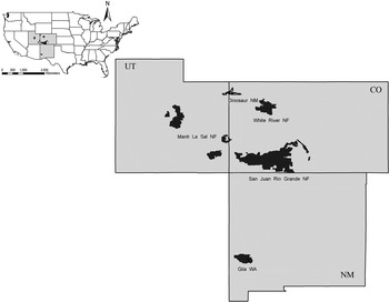
Baseline sites for this study were located in three adjacent Intermountain Area states: Colorado, Utah and New Mexico (Fig 1). All four study areas (San Juan–Rio Grande National Forest, Colorado, Dinosaur National Monument, Utah-Colorado, Manti La Sal National Forest, Utah, and the Gila Wilderness Area in the Gila National Forest, New Mexico) have unique vegetation types, complemented by significant variation in geological substrata as well as temperature and precipitation patterns. Overall temperature and precipitation values for the region are highly variable (Table 1). This combination of environmental conditions results in a wide variety of habitat types which often support diverse and complex lichen communities.
Map showing data collection and field validation areas. Data from Dinosaur National Monument, Gila Wilderness Area, Manti La Sal National Forest, and San Juan-Rio Grande National Forest were used to calibrate the Model and it was validated using sites in the White River National Forest.

Range of annual precipitation and temperature for the four study areas

Data collection
In total we used 72 air quality bio-monitoring baseline sites for our study: 32 in the San Juan-Rio Grande National Forest, 18 in Dinosaur National Monument, 15 in the Manti-La Sal National Forest, and 7 in the Gila Wilderness Area. All baseline sites were initially established between 1991 and 1999 as part of a comprehensive regional air quality bio-monitoring programme. The Regional Air Quality Bio-Monitoring Program is a long-term project supported by the USDA Forest Service and National Park Service. The programme specifically targets protected airsheds such as wilderness areas and national parks. At each of the study areas baseline sites were selected in consultation with USDA Forest Service or National Park Service personnel, with careful attention paid to any local potential sources of air pollution. A few of the baseline sites had experienced some air pollution-related impact; therefore, initial sampling (overall species diversity, occurrence of sensitive indicator species, levels of air pollutants in tissues of sensitive indicator species, etc.) was used to determine impact levels for more effective future monitoring of those sites. However, generally most of the baseline locations were clean air sites each covering an area of about 1 hectare. At each site, all available substrata were carefully examined. If U. hirta was reported for a given site, that site was designated as a ‘present’ site. Voucher specimens are deposited in the lichen herbarium at Brigham Young University (BRY).
Predictor variables
Since we used a previously collected dataset (lacking data concerning environmental parameters) to construct our model, our predictor variables are GIS derived variables prepared using ArcGIS 9.3 (Environmental Systems Research Institute) software. Four geographical variables (elevation, aspect, slope, and land forms and uses) and five macroclimatic variables (average monthly rainfall, average monthly minimum temperature, average monthly maximum temperature, integrated moisture index, and solar radiation) were used in developing our predictive model.
Elevation, slope and aspect
An elevation gradient of 1 Arc Second (30 m) was acquired from the National Elevation Dataset (NED), United States Geological Survey (USGS). Elevation of the baseline plots in the four study locations ranged between 1490 and 3860 m. Using the Spatial Analyst tool in ArcGIS 9.3 software (ESRI), NED was filled to remove pits and peaks in the dataset which may cause small imperfections in the output data. Using the filled NED data, aspect and slope data were generated using the Spatial Analyst extension in ArcGIS. Percent slope of these baseline plots ranged from 0 to 38°. Aspect was reclassified into four classes: North (315°–45°), East (45°–135°), South (135°–225°), and West (225°–315°).
Solar radiation
Solar radiation was generated from NED data by using Spatial Analysis. Default values were accepted for all designated parameters. According to Coxson & Stevenson (Reference Coxson and Stevenson2007), maximum growth rates for lichens occur between March and October in British Columbia. The ideal growth time frame for lichens in the Intermountain Area will probably vary somewhat from the Coxson & Stevenson prediction; however, it clearly falls within the period of March to October due to the critical metabolic dynamic between appropriate temperature and availability of moisture. Therefore, solar radiation (W/m2) layers for the months including March through to October for one year were generated and averaged for each of the four study areas. Because of relatively constant solar radiation values in different years we opted to use just one year.
Integrated Moisture Index (IMI)
Moisture availability is also an important predictor variable because lichens take water up directly from the atmosphere. Iverson et al. (Reference Iverson, Dale, Scott and Prasad1997) developed a raster based image called the Integrated Moisture Index which is used for estimating potential soil moisture availability across a heterogeneous landscape. To produce IMI images three topographic features, hillshade, flow accumulation, and curvature were derived from NED data. Hillshade is an index of the drying effects of differential solar radiation due to variation in slope angle, aspect and position, and shading from adjacent cells. Curvature measures convexity and concavity across landscape. Flow accumulation is a count of the number of cells that contribute water down slope to an evaluation cell. All three raster layers were rescaled to 0–100 ranges and finally combined into a single layer using the equation in the raster calculator function of Spatial Analyst.
IMI=(hillshade×0·5)+(curvature×0·15)+(flow accumulation×0·35)
The Integrated Moisture Index ranges from 0 to 100, with 0 indicating no moisture accumulation and retention and 100 indicating the highest moisture accumulation and retention.
Land forms and uses
Vector data for land use was acquired from the United States Geological Survey (USGS) website which was later converted to 30 m2 raster data for analysis in ArcGIS. Our study sites included broad categories of land type ranging from forest to shrubland to tundra vegetation. However, most of our study sites were in evergreen forested landscapes followed by shrub rangelands and mixed rangeland types.
Temperature and precipitation
Average monthly maximum temperature (°C), average monthly minimum temperature (°C), and average monthly precipitation (cm) data at 1-km resolution for the months of March through to October of the climatological period 1971–2000 were obtained from Parameter-Elevation Regressions on Independent Slopes Model (PRISM; PRISM Climate Group, Oregon State University). All raster datasets used in the analysis were re-sampled to a 30-m resolution. For this study, the average monthly minimum and maximum temperatures, and precipitation for the period of March to October were used for all analyses. This time frame represents the maximum growth period of lichens (Coxson & Stevenson Reference Coxson and Stevenson2007).
Data preparation
GIS layers representing each study area were generated and the GPS coordinates for all sites with their response variables were plotted in their respective layer. A 55 m circular buffer was created around each reference point to roughly represent c. 1 ha of sample area surrounding each response variable. Then predictor variable statistics for each response variable location was calculated using the Zonal Statistics function in ArcGIS 9.3.
Analysis
Non-parametric multiplicative regression analysis (NPMR) was used to analyze and develop predictive models using the Hyperniche v1 software developed by McCune & Mefford (Reference McCune and Mefford2004). NPMR models how a species' distribution relates to environmental factors across a study region in order to estimate the probability of the species' occurrence at new sites. Species seldom respond linearly to an individual factor. Hence, a species' occurrence across a landscape is determined by a complex interplay of various environmental factors. But traditional parameterized models such as linear regression cannot capture the complexity of a species' relationship to its habitat. On the other hand, NPMR uses a kernel weighting function to select the best predictor variables based on their relationship to species' occurrence or abundance. Further, NPMR effectively represents species responses to multiple habitat factors and the interactions among factors are accommodated automatically. Further NPMR has a built-in cross-validation procedure to reduce problems of overfitting so it fits the model better and more parsimoniously than other traditional methods.
Habitat modelling using NPMR generally has two phases, calibration and application. In the calibration phase, empirical data based on species abundance or presence-absence are used to build the model in order to more effectively estimate abundance or likelihood of occurrence based on the predictor variables. During the calibration phase, the most powerful subset of predictor variables is identified and smoothing parameters or tolerance, the standard deviation of the Gaussian weighting function for each predictor, for the quantitative variables are determined. The resulting habitat model is used in the application phase to predict species' occurrence or abundance at unknown sites.
In this study, habitat models were constructed using a local mean (LM) with Gaussian weighting. This is a stepwise free search function which seeks a range of models with different combinations of predictors. Model quality is assessed by the descriptive statistic log β, which is the log likelihood ratio for two competing models (McCune Reference McCune2006). The log β is calculated as the log10 of the ratio between the developing NPMR model, or ‘posterior’ model, and the naïve or prior model. This prior model is simply the average frequency of the species in the full dataset. A predictor variable was retained only when its inclusion increased the log β value of the posterior model by at least 5% over the next largest model.
To compare whether the default minimum average neighbourhood size (3·6 which is 5% of total sampling units) was appropriate for the study we also developed another model with a neighbourhood size of 10 (14% of the sample size). Neighbourhood size can be defined as the sum of weights or amounts of data used to calculate the estimated response at any given point, and the average neighbourhood size is simply the sum of neighbourhood sizes for all plots divided by the total number of plots; this value decreases with the increase in number of variables (Yost Reference Yost2006). After the best model was selected, it was then fine-tuned, which involved adjusting the continuous variable tolerances by 1% of the variable's value range. The model with the highest log β value is considered the best model. We also did sensitivity analysis to evaluate the relative importance of particular parameters, that is, predictor variables within the model. This is particularly important because with NPMR we do not have a fixed coefficient or slopes that we can compare in size. In this analysis we calculated sensitivity values for each predictor which are related to the importance of variables. So, the greater the sensitivity, the more influence that variable has in the model (McCune Reference McCune2006). Models with log β values higher than 2·0 provide decisive evidence against the naïve model (Jeffreys Reference Jeffreys1961). We also evaluated our models on the basis of percentage improvement over the naïve model. The percent improvement is calculated by dividing the sum of the number of plots with improvements by the total number of plots. Improvement is represented by plots having estimates of the probability of encountering a species in the study areas either higher than the naïve model when species are present, or lower than the naïve model when species are absent (Yost Reference Yost2008). The resulting models were further evaluated with a Monte Carlo permutation test with 1000 randomized runs. Finally, using the GIS function in Hyperniche, a predictive map was generated for the model with the highest log β values.
Model validation
The reliability of the model generated was tested for the western portion of White River National Forest. This area was not included when we established the original input variables. The model generated a predictive map with a range of values related to the probability of occurrence of U. hirta. The values were first normalized to the range of 0–1 and then classified into ten probability classes using the natural breaks function in ArcMap. These probability classes were reclassified into: a low probability class with values ranging between 0–0·35, a mid-probability class with a range of 0·35–0·65 and a high probability class with a range of 0·65–1·00. Ninety points were randomly selected in the White River National Forest validation area using Hawth's Tool in ArcGIS. However, when we started our fieldwork we found many of our sites were inaccessible. Due to the large number of inaccessible areas in the forest, and also time constraints, we adjusted some of our points in more accessible areas in order to complete the project promptly. Each accessible field validation point was visited and occurrence of the test species was checked. We used the same survey method in the field that was employed in the original survey. Hence, at each validation point 55 m transects were walked in the four cardinal directions covering an area of c. 1 ha. Sites were classified based on the number of U. hirta encounters. Sites with 10 or more total encounters were designated as abundant, while sites with 4–9 encounters were listed as common and sites with 3 or fewer encounters were designated as rare. Finally, the percentage of sites with U. hirta was calculated for each probability class.
Results
Usnea hirta was present at 30 of the 72 baseline sites. It was common in the San Juan-Rio Grande National Forest (present at 19 sites out of 32) and the Gila Wilderness Area (present at all 7 sites), but rare in Dinosaur National Monument (3 out of 18 sites) and the Manti La Sal National Forest (1 out of 15 sites).
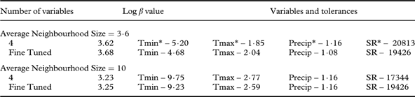
Using the default average neighbourhood size of 3·6, the model with the highest log β value (3·62) included four variables: average monthly minimum temperature, average monthly maximum temperature, average monthly precipitation, and average monthly solar radiation (Table 2). The best model was then fine-tuned which increased the log β value to 3·68. To determine which of the predictor variables is most important in predicting the distribution we calculated a sensitivity value for each of the predictor variables and the values were 0·11, 0·71, 0·63, and 0·63 for average monthly minimum temperature, average monthly maximum temperature, average monthly precipitation and average monthly solar radiation, respectively. Hence, from the sensitivity value we can say that average monthly maximum temperature was a more influential predictor in this model for the prediction of Usnea distribution.
Probability Model selected as best modelling approach for Usnea hirta with different average neighbourhood sizes
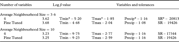
* Tmin=average monthly minimum temperature; Tmax=average monthly maximum temperature; Precip=average monthly precipitation; SR=average monthly solar radiation
Of the 30 sites where U. hirta occurred, 20 showed improvement over the naïve model, having estimates higher than the naïve model. Similarly, for the plots where U. hirta was absent (42 sites), 29 had estimates lower than the naïve model, thus showing improvement over the naïve model. Overall, the improvement was 68·1% (49 out of 72 sites). Our best model was statistically significant (P<0·01) when evaluated using a Monte Carlo permutation test (1000 randomized runs).
When average neighbourhood size was set at 10, the same four variables (average monthly minimum temperature, average monthly maximum temperature, average monthly precipitation, and average monthly solar radiation) emerged as the best predictors with a log β value of 3·23 (Table 2). In this model, average monthly precipitation (sensitivity=0·64), was relatively more important than average monthly minimum temperature (sensitivity=0·03), average monthly maximum temperature (sensitivity=0·61) and average monthly solar radiation (sensitivity=0·27). When the model was fine-tuned there was only a 0·02 unit increase in the log β value (3·25). The overall improvement percentage over the naïve model was 69·4%. Our best model showed a statistical significance of P=0·05 when evaluated using a Monte Carlo permutation test with 1000 randomized runs. Although the model with an average neighbourhood size of 10 showed better overall improvement, we selected the model with an average neighbourhood size of 3·6 for generating the predictive maps because it had a higher log β value and significance level (P<0·01).
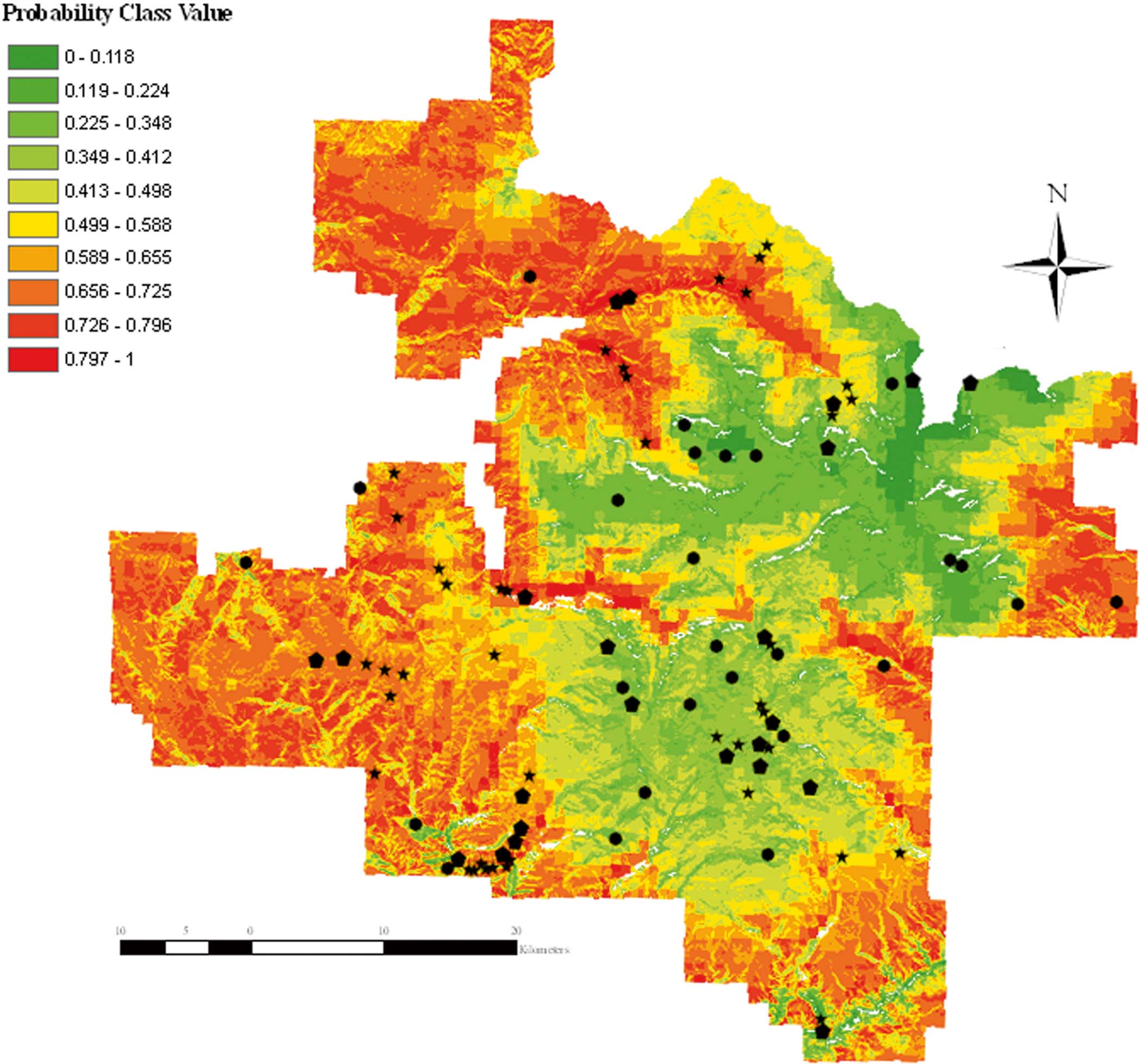
The predictive map generated using Hyperniche is shown in Fig. 2. The predictive map for U. hirta mapped 96% of the total land area of White River National Forest, while 4% of the land area occurred below the minimum neighbourhood size so there are no predictive values for these areas and therefore they appear white in the map (Fig. 2). Out of the possible 90 points we visited 64: 11 low probability, 26 medium probability, and 27 high probability. In the low probability area U. hirta was present at 5 sites (45·5%), and in 17 (65·4%) and 19 (70·4%) of the medium and high probability sites, respectively (Fig. 2).
Distribution map for Usnea hirta in the White River National Forest. Black stars represent sites where U. hirta was recorded, black pentagons represent sites with no U. hirta and black circles represent inaccessible sites. White areas represent no data value which is due to lower average neighbourhood size.
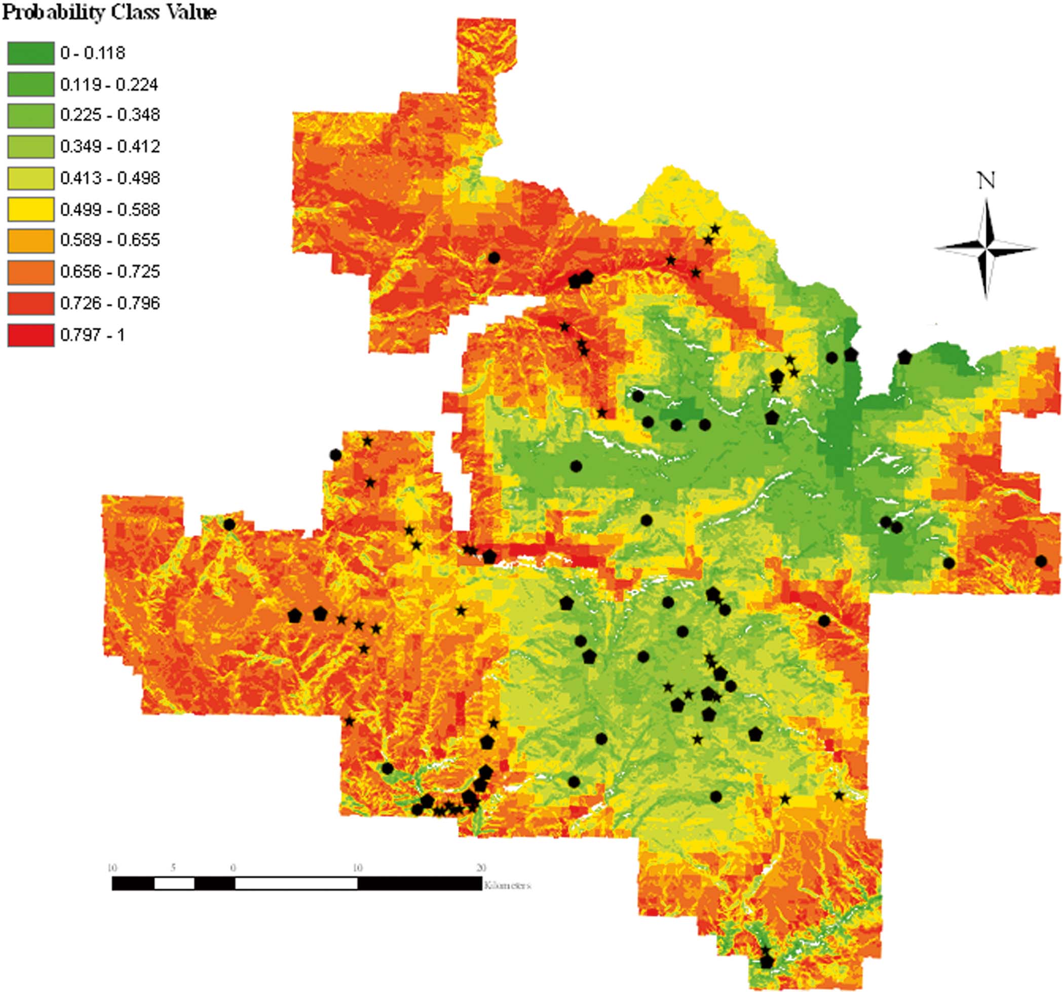
The predictive map suggested that the high probability areas were generally located in the north-east and western parts of the forest. During the field validation phase of this study, we were able to document the occurrence of U. hirta in most of these areas.
Discussion
This study demonstrates the usefulness of ecological niche-based modelling to predict the distribution of an air pollution-sensitive lichen species based on geographical and climatic variables. In this study we used the non-parametric regression method (NPMR) because it readily models nonlinear species abundance-habitat relationships, automatically considers interactions among predictors, and, by combining the effects of predictors multiplicatively, potentially better accounts for the effects of unacceptable habitat conditions on species abundance than do additive modelling techniques (McCune Reference McCune2006).
Our model showed that U. hirta has a high probability of occurring across a large portion of the White River National Forest and our field collections documented that U. hirta occurred in 70% of the sites sampled in the high probability areas of the forest. Usnea hirta also occurred at a higher than predicted frequency in the low (0–0·35) and medium (0·35–0·65) probability areas of the forest; however, the occurrence rate was low. High probability locations for U. hirta, predicted by the model, ranged between 2400 and 3000 m. In our field surveys we consistently found that sites within this elevation range demonstrated abundant quantities of U. hirta. We also found that U. hirta occurred with much lower frequency above and below the high probability elevation range; a logical conclusion in light of the fact that the most common substratum for U. hirta was conifer species such as Abies concolor and Picea engelmanii which were abundant in the above mentioned range in the White River National Forest.
The results of our study suggest temperature, precipitation, and solar radiation are important variables governing the distribution of U. hirta, which agrees with several similar studies concerning distribution of lichen species (Dietrich & Scheidegger Reference Dietrich and Scheidegger1997; Glavich et al. Reference Giordani2005; Werth et al. Reference Werth, Tommervik and Elvebakk2005; Ellis & Coppins Reference Ellis and Coppins2006; Giordani & Will-Wolf Reference Glavich, Geiser and Mikulin2006; Bolliger et al. Reference Bolliger, Bergamini, Stofer, Kienast and Scheidegger2007; Giordani Reference Giordani and Will-Wolf2007; Radies et al. Reference Radies, Coxson, Johnson and Konwicki2009). Out of our four primary predictor variables, sensitivity analysis identified maximum temperature (sensitivity=0·71) as the best predictor variable for the distribution of U. hirta. According to McCune (Reference McCune2006), the greater the sensitivity, the more influence that variable has in the model. In the White River National Forest the distribution of U. hirta is generally limited to subalpine coniferous forests (2400–3000 m) with filtered sunlight, cool summer temperatures, and abundant winter and summer moisture.
In part, the limitations in our model may be related to the misidentification of species. We assumed that the species used in developing our model had been correctly identified; however, recent molecular studies of various lichen genera suggest that species delimitation is far more complex than previously thought (Leavitt et al. Reference Leavitt, Johnson, Goward and St. Clair2011). There may have been similar issues in distinguishing between various Usnea species based on conflicts between the application of traditional taxonomic characters and molecular data. While field testing our model we encountered what appears to be U. lapponica at some sites. As both U. hirta and U. lapponica have somewhat similar habitat preferences and are both sensitive to various air pollutants, we recorded all sites with U. lapponica as positive records for U. hirta. This loss of taxonomic resolution may have resulted in a general failure to effectively identify appropriate tolerances for predictor variables during the calibration phase of this project.
Another limitation of this study involved the structure of the database used to develop the ecological models. The original dataset was not collected with the intention to model lichen species distribution; rather it was collected as part of a floristic and air quality bio-monitoring survey. Therefore, the variables used in the original database for predicting lichen species' occurrence were based strictly on GIS derived data. Designing an appropriate sampling procedure is an important aspect of modelling species distribution since the selection of explanatory variables as well as the prediction accuracy of the model generally depend on the sampling strategy for each dependent variable(s) (Edwards et al. Reference Edwards, Cutler, Zimmermann, Geiser and Moisen2006). Our model has certainly performed better than expected but would likely have been much more effective if our sampling design had been based specifically on the modelling of lichen species distribution.
Field-measured variables such as total tree basal area, number of tree species colonized by lichens, proportion of trees including deciduous trees, canopy cover, vegetation characteristics are key variables for effectively modelling the distribution of lichen species. Research by Hyvärinen et al. (Reference Hyvärinen, Halonen and Kauppi1992) and Gustafsson et al. (Reference Gustafsson, Appelgren, Jonsson, Nordin, Persson and Weslien2004) emphasized the importance of field-measured variables in accurately determining the distribution of lichen species. Similarly, Bergamini et al. (Reference Bergamini, Stofer, Bolliger and Scheidegger2007) found that models based on field-measured variables performed better in predicting microlichen richness than models based on climatic variables. Our model would certainly have performed better if we had included field-measured variables in our predictor list along with macroclimatic and geographical variables. Further, the use of macro- rather than micro-climatic variables may have reduced the performance of our model. According to Bergamini et al. (Reference Bergamini, Stofer, Bolliger and Scheidegger2007), using only climatic variables as predictors lowers the performance of the model because of potential mismatches between real climatic and modelled variables; a condition further complicated by the fact that lichens are inherently more sensitive to microclimatic conditions. Finally, we predicted the distribution of species beyond the range of the climatic data used to calibrate our model. According to Thuiller (Reference Thuiller2004), model application becomes more uncertain outside the climatic range of the calibrated dataset.
In spite of these limitations, our predictive model consistently provided useful information about the distribution of U. hirta in the White River National Forest. In light of intensive fossil fuel development and processing in this region over the last 10 years, protection of the Flat Tops Wilderness (White River National Forest), a federally protected airshed, has become increasingly important. Our model also indicated that more emphasis should be placed on the north-east and western parts of the White River National Forest when establishing future air quality bio-monitoring baseline sites using U. hirta as the sensitive indicator species. The use of air pollution-sensitive species, such as U. hirta, provides an early indication concerning potential air pollution-related damage to critical ecosystem components. This advantage becomes particularly important in wilderness areas with a federally mandated expectation for pristine environmental conditions. Consistent bio-monitoring of air quality with periodic reviews (every 10 years) in protected forest systems, using air pollution-sensitive lichen species such as Usnea hirta, shows promise in helping land managers formulate effective and efficient plans for monitoring and maintaining forest health. Furthermore, this model shows promise for effective use across significant portions of the Intermountain western United States.
We express appreciation to the USDA Forest Service for financial support, to Dr Steven Leavitt for field assistance, and to Dr Andrew Yost for his valuable insights, suggestions, and edits, particularly regarding the development of our ecological model. The authors sincerely appreciate invaluable feedback from the reviewers of this manuscript.