I. INTRODUCTION
Fire control radars usually are active only for short time periods and represent severe threats to fighter aircraft. Using onboard electronic support measures (ESM) receivers, the threat signals can be detected and measured. It would be of a high tactical value if these ESM receivers had the capability to obtain a high-accuracy emitter position estimate almost instantaneously.
In order to obtain accurate position estimates of radar emitter, it is crucial to have accurate position and time synchronization among the cooperating platforms. Clocks and platform positions can be synchronized with a theoretical relative accuracy of the order of 10 ns and 5 m using common view GPS (see [Reference Bradford, Parkinson and Spilker1]). Furthermore, precision crystal and rubidium clocks are now commercially available mitigating the requirements for precise clock synchronization. Reference emitters with well-known positions can also be a complement to GPS for synchronization of clocks and platform positions.
The time of arrival (TOA) of intercepted radar pulses can theoretically be measured with an accuracy of  . In practice, an accuracy of around 10 ns is expected. The phase change of a signal during a 10 ms radar illumination typically can be measured with an accuracy of around 20° which corresponds to a frequency measurement accuracy of around 10 Hz.
Assume that the time difference of arrival (TDOA) of a pulse to two ESM systems can be measured with an accuracy of the order of 15 ns which corresponds to a distance difference of 4.5 m. Using multi-platform (MP)-TDOA with an ESM platform separation of 1 km the bearing to the emitter then can be obtained with an accuracy of around 0.3° in the normal direction to the platform separation line. With more than two platforms the 2D emitter position can be estimated. An introduction to TDOA emitter geolocation can be found in Wiley [Reference Wiley2].
For MP frequency difference of arrival (MP-FDOA) the orientation of the line of positions and the accuracy is strongly dependent on the platform relative trajectories. Assume that two ESM platforms move 1 km after each other with a speed of 300 m/s and that the FDOA to the platforms can be determined with an accuracy of around 10 Hz at 10 GHz. In the normal direction to the line between the platforms this corresponds to a bearing difference of 0.06°. At a range of 10 km from the emitter the range can then be estimated with an accuracy of the order of 100 m. FDOA geolocation is discussed in Wiley [Reference Wiley2].
In order to obtain a good range estimate, the measuring ESM platforms must have a rather large separation. Measurement of TOA and frequency on the same pulses implies that some of the ESM platforms will perform their measurements in the radar sidelobes that require a very high sensitivity. The objective of this contribution is to discuss how such a high sensitivity can be obtained and how high-accuracy measurements still can be obtained.
In Section II, ESM receiver sensitivity requirements are motivated from a scenario example. With a channelized receiver with narrowband receiver channels a basic good sensitivity can be obtained. The use of antennas and signal processing in order to improve the sensitivity is discussed in Sections III and IV, respectively. Processing management and methods to measure signal parameters for weak signals are then considered in Section V. After a discussion in Section VI, the conclusions are finally summarized in Section VII, which is followed by a list of references.
II. SENSITIVITY REQUIREMENTS
A modern fire control radar using pulse compression can be expected to have an output power Ptr = 1 kW and a mainbeam antenna gain G tr = 35 dB. The effective aperture area of an ideal isotropic antenna at a frequency f = 10 GHz is given by A iso = λ2/(4π) = 0.72 cm2. At a range R = 20 km the power received by such an ideal isotropic antenna is then given by P rec = P trG trA iso/(4πR 2) = −43 dBm. The sidelobe antenna gain of a radar can be expected to be 35–40 dB below the mainlobe antenna gain. In a sidelobe of the radar in our scenario example the power level can hence be expected to be down to around −80 dBm for an ideal isotropic antenna. In a real scenario there would be very large variations. For example, one could require a detection range that is up to a factor 10 larger. This would result in a sensitivity requirement that is 20 dB higher. Another important factor to consider is the output power of the radar which in many important cases could be a factor 100 larger implying 20 dB lower requirement on the sensitivity.
Consider a channelized receiver (see [Reference Tsui3]) with B = 20 MHz channel bandwidth and a noise and loss factor F = 15 dB. Then, the sensitivity is given by P min = kTFB·SNR min = −73 dBm. Here, kT = −174 dB (mW/Hz) is the product of Boltzmann's constant and a reference temperature, and SNR min = 13 dB is a minimal signal-to-noise ratio (SNR). The boresight gain of a wideband widelobe antenna is around 0 dBi and around −20 dBi at 90° from boresight.
In order to detect and measure important threat radars in their sidelobes, an extra sensitivity improvement of at least around 10 dB is required. The sensitivity can be improved by using a directional antenna, two antennas, signal integration, or a matched filter. Different methods to detect weak signals are also discussed in Tsui [Reference Tsui4] and Pace [Reference Pace5].
III. USE OF ANTENNAS
A) Directional antennas
A wideband phased array antenna covering a frequency 3:1 ratio with 8 × 8 elements could be a suitable alternative to obtain extra sensitivity. With an antenna element separation of λ/2 at the highest frequency the antenna width would be 4λ. Then at the highest frequency the beamwidth would be around 15° and the gain would be 23 dBi. At the lowest frequency, the beamwidth and the gain would be around 45° and 13 dBi. With a frequency coverage of 6–18 GHz such an antenna would have an aperture width of 6.7 cm. A drawback with wideband phased arrays is their complexity and that they have a limited instantaneous field of view. Hence, precise synchronization between the platforms is required in order to focus the antennas toward the threat under investigation. This does, however, require some knowledge of the position of the threat, something which may not be available.
B) Two antennas
An alternative to a phased array is to use two separate equally directed antennas and two separate receivers. The noise and loss factor of a wideband receiver usually is of the order of 15 dB. Hence, the internal noise in each receiver dominates the noise in the received signals. Now let us consider the signals from the same frequency channel for the two antennas. The signals received from a certain emitter will then be the same except for a constant phase difference and the two essentially independent receiver noises. In order to detect a signal one of the antenna signals is down-converted by the other and low-pass filtered.
Pulsed radar signals usually have no modulation, linear frequency modulation (LFM), binary phase shift keying (BPSK), poly-phase coding including digital variants of LFM, or more random complex frequency modulation such as Costas codes. The pulse width and the bandwidth of typical modulated radar pulses can be expected to be 3–10 µs and 1–10 MHz, respectively. This means that LFM pulses have a frequency derivative of 0.1–3 MHz/µs.
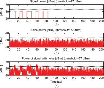
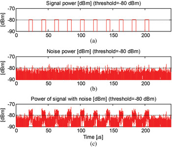
In Fig. 1, a set of −80 dBm pulses from a 20 MHz receiver frequency channel is shown, the receiver noise and the sum of the ideal signal and the noise. The three first signals have LFM with bandwidths of 5, 10, and 10 MHz and pulsewidths (PWs) of 3, 5, and 10 µs. The fourth signal has a binary phase modulation with 31 subpulses with 150 ns length each. The two last pulses are short unmodulated pulses with PWs of 1 and 0.5 µs. The noise floor reference is at −77 dBm. In the frequency channel, all carrier frequencies are equal to 4 MHz.
(a) Ideal received signal power in dBm. (b) Noise power in dBm. (c) Power of signal and noise.

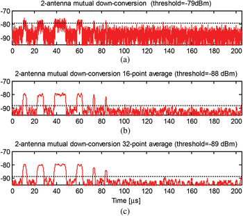
In Fig. 2, the down-conversion of one antenna signal with the other is shown with 1-, 16-, and 32-point averaging. All −80 dBm signals can be easily seen above the noise background. The noise floors are at −79, −88, and −89 dBm. This corresponds to processing gains of 2, 11, and 12 dB. The TOA of the pulses can be expected to be measured with an accuracy of around 100 ns for the case with 16-point averaging.
(a) 2-antenna signal mutual down-conversion. (b, c) Down-conversion and 16- and 32-point averaging.

If the antenna separation is short the phase of the down-converted signal can be used for estimation of the angle of arrival of the received signal. The major drawbacks with this approach are that it requires twice the hardware resources and space compared to a single-channel approach and that the sensitivity will be dependent on the direction to the threat.
III. USE OF SIGNAL PROCESSING
A) Short-time Fourier transform (STFT)
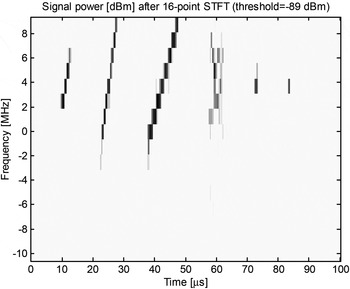
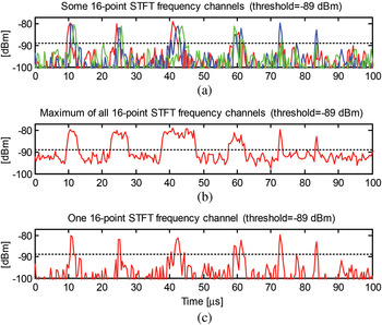
Typical threat LFM pulses have a frequency derivative of 0.1–3 MHz/µs. Hence, a receiver could use an STFT with a frequency resolution of around 1 MHz to create a time-frequency (TF) representation of the received signal. The next step could then be to search for patterns in this TF picture with an energy above a suitable threshold. In Figs 3 and 4, a 16-point STFT of the noisy −80 dBm signal in Fig. 1 is shown. Here, we can clearly see the time-dependent instantaneous frequencies for the three LFM pulses. The BPSK pulse has an instantaneous spread of its power and the short unmodulated pulses are concentrated in frequency. The noise floor is at −89 dBm which corresponds to a processing gain of 12 dB. The TOA of the pulses can be measured with an accuracy of around 100 ns.
Signal power in dBm after a 16-point STFT.

(a) Some 16-point STFT frequency channels. (b) Maximum of all frequency channels. (c) One of the frequency channels.

B) Signal squaring
Let us now consider a BPSK signal in a 20 MHz frequency channel. Such a signal can be expressed as

Here,  is the signal in the frequency channel, A is the amplitude,
 is the binary phase modulation signal,
 is the carrier frequency,
 is a phase, and
 is the noise that we assume to be additive. After squaring the signal and using
 we obtain

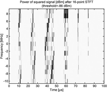
A 16-point STFT for the square of the noisy simulated signal in Fig. 1 is shown in Fig. 5. The fourth signal around the time 60 µs is the square of the squared signal  . The first term in the squared BPSK signal is an unmodulated sinusoidal signal with a frequency that is twice the original carrier frequency. In Fig. 5, this signal can be seen as an enhancement at the doubled carrier frequency 8 MHz. The second term is the product of the original binary phase-modulated carrier signal and the noise. This will result in a noisy spread spectrum signal during the pulse duration. The spread spectrum signal can be seen in Fig. 5 spread among all frequencies during the pulse duration. The third term is squared complex noise which will be enhanced if the SNR is large.
16-point STFT of the square of the received noisy signal.

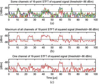
In the TF picture shown in Figs 5 and 6, the beginning and end of each pulse is easily seen. The LFM pulses have doubled frequency ridges due to frequency folding of the doubled frequency. The BPSK pulse has a frequency ridge with constant frequency. Measurement of the carrier frequency will be ambiguous in this case. The noise floor is at −86 dBm which corresponds to a processing gain of 9 dB.
(a) Some channels of 16-point STFT of squared signal. (b) Maximum of all channels. (c) One of the channels.

C) Correlation with a delayed signal
Costas codes can be seen as LFM pulses where subpulses have been randomized in time. In order to detect Costas-coded pulses, we have to use more general methods. Radar pulses are often transmitted as a train of coherent equal pulses. In such a case, one can correlate the received signal with a delayed copy of the signal. There will then be a pronounced peak for a delay that is equal to the pulse repetition interval (PRI). With an integration time of 1 µs there will be a processing gain of around 10 dB.
D) Matched filter method
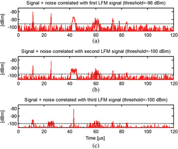
In a typical scenario, at least one of the ESM platforms is illuminated by the radar main beam. Then the radar waveform can be measured at a high SNR and the parameters of the received pulses can be sent to the cooperating ESM platforms. These parameters can be used to compute pulse templates. The noisy received signal at the cooperating ESM platforms can then be correlated with these templates and obtain a large processing gain. This of course requires that the pulse waveform does not change. In Fig. 7, the received noisy −80 dBm signal in Fig. 1 is correlated with noise-free copies of each of the three LFM pulses. The TOA of the pulses here can be measured with an accuracy of around 25 ns.
Correlation of the noisy received signal with ideal templates of the first (a), second (b), and the third (c) LFM pulses.

E) Video filtering
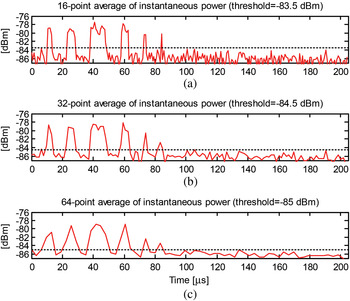
If the SNR in the 20 MHz frequency channel is larger than 0 dB then low-pass filtering can increase the sensitivity. In Fig. 8, the 16-, 32-, and 64-point averages of the instantaneous power of the received noisy signal from a 20 MHz frequency channel from Fig. 1 are shown. The five pulses are all easily seen.
16-, 32-, and 64-point averages of the instantaneous power.

The noise floors are at −83.5, −84.5, and −85 dBm corresponding to processing gains of 6.5, 7.5, and 8 dB. If a pulse is detected the corresponding samples can be stored for a while in a short-term memory.
If a pulse template is available within a few seconds then important signal parameters can be measured with better accuracy using cross correlation of the signal and the pulse template.
IV. PROCESSING MANAGEMENT
A) Detect, decide, store, and sort
In important possible scenarios, a sensitive receiver system will intercept radar pulses at a very high rate. Hence, the real-time processing load on a digital receiver will be very high and therefore it is important to reduce the data rate in the receiver system as soon as possible.
The first step in the signal processing chain is to detect whether there is signal power which is significantly over the background noise level. In a high-sensitivity receiver, there will be a lot of signals of interest and a lot of interfering signals which are not of interest and sometimes also spurious false signals that are artifacts due to imperfect receiver performance.
For each detected piece of energy, a decision must be made with a very short delay if a detected possible pulse is of interest. In order to have a basis for such a decision a rough characterization of the possible pulse must be performed. This means that provisional measurements of at least a few basic pulse parameters such as TOA, PW, radio frequency (RF), and power amplitude (P) must be performed immediately after detection. Using such a characterization a temporary decision may be taken if the pulse under consideration is worth a further investigation or if it is not of interest.
Assume that a certain probable pulse is decided to be of interest. From the provisional measurements it is clear in which narrowband receiver channel that the probable pulse has been found and during which time interval. The corresponding digital data samples are then stored together with the provisionally measured pulse parameters. Radar pulses have a PW typically from 100 ns to 10 µs. With a channel sampling rate of 40 MHz this corresponds to 4–400 samples for each pulse. Stored provisional pulse data are then sorted into trains of pulse descriptions with similar parameter values.
B) Pulse ensemble processing
Radars in general send bursts of almost identical pulses with constant PRIs  . A received complex channel signal consisting of a pulse sequence and additive noise can be written as

Here,  is a generic pulse signal,
 is the separation in time,
 is the pulse amplitude,
 is the difference in phase between two consecutive pulses, and
 is the additive noise.
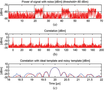
Assume that such a pulse sequence fulfilling some decision criteria is intercepted by the receiver. Then the channel samples of the corresponding pulse are expected to be sorted into an ensemble of similar pulses. In Fig. 9(a), ten simulated ideal LFM pulses are shown. In Fig. 9(b), simulated receiver noise is shown and in Fig. 9(c) a simulated received noisy signal is shown.
(a) The first four of 30 noisefree LFM pulses. (b) Noise. (c) Pulses and noise.

The first step in the processing of such a pulse ensemble is to measure the difference in TOA and phase of arrival (POA) of the pulses. The pulse in the ensemble that has the highest energy is used as a pulse template or pulse reference (see Fig. 10(a)). The pulse template is then correlated with all other pulses in the ensemble (see Fig. 10(b)). In such a pulse correlation, the complex pulse samples are multiplied by the complex conjugate of the complex pulse template samples for different delays and summed. The delay that gives the highest correlation is considered as the time delay between the pulse and the pulse template. An example of a correlation peak is shown in Fig. 10(c). In this way, the separations  in time between the pulses are estimated. The phases of the cross-correlations at the maximum are considered as the phase differences
 between the pulses and the pulse template.
(a) Extraction of a reference pulse. (b) Correlation of pulses with reference pulse. (c) One correlation peak for correlation with ideal and with noisy template.

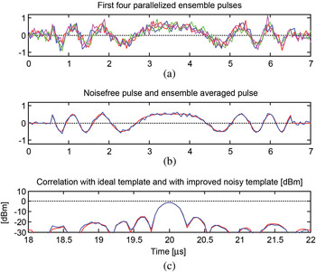
The second step in the processing of a pulse ensemble is to align the pulses in time and phase. A pulse is aligned in time by subtracting the time difference between the pulse and the pulse template. Then the pulse is aligned in phase by subtracting the phase difference between the pulse and the template from the pulse phase. Examples of such aligned pulses are shown in Fig. 11(a).
(a) The first four parallellized ensemble pulses. (b) Noise-free ideal pulse and ensemble averaged pulse. (c). One peak for correlation with ideal and with noisy template.

An improved pulse template is obtained by computing the average of the time- and phase-aligned ensemble pulses for each sample (see Fig. 11(b) and Langley [Reference Langley6]). The standard deviation for the averaged pulse in linear scale is improved by a factor  where N = 10 is the number of pulses in the ensemble in the example. This corresponds to an improvement of the SNR in power scale by a factor of N = 10 = 10 dB. Such an improvement can only be obtained if the ensemble pulses have been aligned well enough.
From the sample-by-sample averaging of the aligned ensemble pulses, an improved pulse template is obtained. This improved pulse template is then correlated along the original received channel signal. This is similar to pulse compression in a radar receiver. At certain delays when the pulse template matches to a received pulse there will be a correlation maximum. The TOA of the pulse can then be measured with high accuracy as the time position for the start of the pulse template. The POA is measured with high accuracy from the phase of the correlation peak. From the relative phases of the pulses in the train high-accuracy estimates of the frequency of arrival (FOA) can be estimated. Pulse-shape parameters can be measured with high accuracy on the improved pulse template. By exchanging TOA and FOA measurement data between platforms high-accuracy estimates of the emitter positions can be obtained (see [Reference Wiley2]).
V. DISCUSSION
The optimal way to obtain high sensitivity and perform high-accuracy measurements would probably be to use a wideband phased array antenna with a gain of 15–25 dB combined with a channelized digital receiver with a channel bandwidth of 10–20 MHz. The drawbacks with such a solution are high complexity, high cost, and that all contributing antennas must be pointing toward the same area of interest at the same time.
Using 16-point STFT for selected 20 MHz channels is quite a good alternative with much less complexity. The processing gain with such a solution is a factor of 16, which equals 12 dB if most of the instantaneous signal power falls into one STFT channel at a time. STFT gives a TF representation of the signal which can be used to measure pulse characteristics.
Pulses with BPSK with short subpulses have a large instantaneous bandwidth and then STFT can be less advantageous although such a pulse can often be seen quite well anyway in the STFT channels. A signal processing complement can be to perform a 16-point STFT on a squared channel signal instead since the binary phase-shifts are erased by the squaring of the signal.
Often a pulse template can be obtained from a signal library or from a cooperating ESM platform. Then the received channel signal can be correlated with this pulse template and for each pulse of that type a narrow strong spike is obtained enabling high-accuracy measurements of TOA and FOA. For a 10 µs pulse and a 20 MHz channel, we will have a processing gain of a factor 200 or 23 dB.
A complement to the more advanced methods could be to use 16-, 32-, or 64-point averaging of the signal power in order to obtain a substantial processing gain of 6–8 dB. The advantage with such incoherent integration is the low complexity of this method.
The samples of the detected pulses can be extracted, stored, and sorted into pulse ensembles. By correlating the ensemble pulses with a reference pulse the PRIs and the phase differences, and hence the frequency can be measured with high accuracy.
VI. CONCLUSIONS
It would be very advantageous for modern fighter aircraft to have a capability of obtaining high-accuracy estimates of the position of important threat radars after a few seconds. This is possible by exchanging high-accuracy measurements of the TOA and FOA of signals to cooperating ESM platforms. This typically requires that some of the ESM platforms have to have sensitivity to detect and measure the signals in the radar sidelobes. After examining a set of possible methods, we can conclude that there are several methods that can give a sensitivity that in many important scenarios will allow measurement also in the radar sidelobes.
ACKNOWLEDGEMENTS
The authors acknowledge support from the European Defense Agency (EDA), French DGA, Swedish FMV, and Italian MOD which have contributed to the funding of this study under EDA contract B-0055-IAP2-ERG.
 Göran Tengstrand received an M.Sc. degree in engineering physics from the Royal Institute of Technology in 1972 and received a Ph.D. degree in theoretical physics from the same institute in 1980. He is now employed by Saab EDS as a specialist in signal processing and has been working for the defense industry mostly with EW systems since 1982. His main research interests are signal processing, radar, and EW technology.
 Peter Hultman is employed by Saab EDS as a project manager. He has worked in various engineering management and system engineering positions at Saab EDS, and he has been responsible for radar and electronic warfare education for the Royal Swedish Navy. P. Hultman received his education in radar and electronic warfare technology from the Swedish National Defense College and Linköping University in 1992.
 Jean-François Grandin had joined THALES company in 1983. He is an expert in electronic warfare systems and has led numerous designs of RWR, ESM, and ELINT information processing. He has published more than 30 papers on related topics: location, classification, radar recognition, system performances analysis, sensors, and data fusion. He had also several teaching activities in applied mathematics.
 Dario Benvenuti graduated in Electronic Engineering in 1998 and in Physics in 2008 at the University of Rome “La Sapienza”. In 1999–2002, he worked in Alenia Marconi Systems (Radar and Technology Division) with main activities concerning analysis and system aspects of a modern multifunctional Phased-Array Radar System. Since 2002, he works in Elettronica SpA in the Analysis Department, where his main activities are the Design and Simulation of data and signal processing algorithms of Electronic Defense Systems. He is the author of several publications concerning Radar and EW.
 Börje Andersson is a senior scientist at the Sensor and EW Systems Division of Swedish Defense Research Agency with more than 30 years of experience in the electronic warfare area. His main professional interests are ESM systems and methods that handle radar emitters.
 Anders M. Johansson was born in 1974 in Sweden. He received M.Sc. in electrical engineering in 2000 and Ph.D. in 2008, both from Blekinge Technical University. He held the position of a research engineer at the Australian Telecommunications Research Institute from 2000 to 2002, and West Australian Telecommunications Research Institute, 2002–2007, developing real-time software for research in the field of acoustic signal processing. Since 2008, he has been at the Swedish Defense Research Agency (FOI). At FOI, he is working in the area of electronic warfare systems. His main fields of interest include sensor array localization and tracking, intelligent support systems, and real-time signal processing.