4.1 Flow past a circular cylinder

The two-dimensional flow past a circular cylinder is considered here. All flow quantities are normalised using the uniform incoming velocity $U_{\infty }$ and the diameter $D$ of the cylinder, which are the reference quantities used for the definition of the flow Reynolds number. Considering a frame of reference with the origin on the cylinder axis, the $x$ -axis parallel to the free-stream velocity and the $z$ -axis with the cross-stream velocity (see for instance figure 1), the dimensions of the computational domain used are the following: $-15\leqslant x/D\leqslant 35$ and $-15\leqslant z/D\leqslant 15$ . The velocity is imposed at the inflow ( $x/D=-15$ ), while stress-free conditions are applied on the lateral boundaries ( $z/D=\pm 15$ ) and on the outflow boundary ( $x/D=35$ ).

The two-dimensional base flow is computed using Nek5000 and employing about 1500 spectral elements of degree $N_{p}=7$ . The same grid is also used for the global stability analysis so as to characterise the onset of the primary instability. In particular, the predicted value of the critical Reynolds number is equal to $Re_{cr}\simeq 46.2$ , which is in close agreement with the literature. For instance, in Giannetti & Luchini (Reference Giannetti and Luchini2007) $Re_{cr}$ is estimated to be $Re_{cr}\simeq 46.7$ .

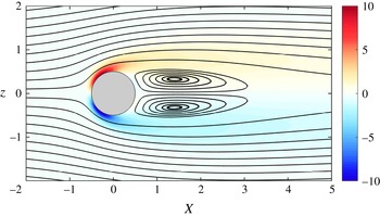
In order to show how the improved local stability analysis (with second-order correction effects included) performs in estimating the global stability properties, we consider the flow in supercritical conditions at $Re=50$ . The corresponding unstable steady state is depicted in figure 1, where the streamline pattern around the cylinder is shown together with vorticity along the $y$ axis. 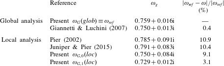The global stability analysis using Nek5000 as a time stepper identifies the leading unstable global eigenvalue, $\unicode[STIX]{x1D714}_{G}(glob)=0.759+0.016\text{i}$ , which is in good agreement with Giannetti & Luchini (Reference Giannetti and Luchini2007), as reported in table 1 for comparison.

Figure 1.

Vorticity (colour) and streamlines of the flow past the circular cylinder at $Re=50$ (streamline spacing in the $z$ -direction is $0.2D$ outside the separation bubble and $0.04D$ in the recirculating region).

Table 1.

Flow past a circular cylinder at $\mathit{Re}=50$ : globally unstable eigenvalue and its prediction by corrected and uncorrected local stability analysis.

When standard local analysis, i.e. without correction, is applied following the indications provided in § 2.2, a region of absolute instability, i.e. where $\unicode[STIX]{x1D714}_{0,i}(X)>0$ , is found in the near wake of the cylinder (not shown here for brevity), which extends in the streamwise direction up to $X\simeq 3.8$ . Since an analytical continuation of the local absolute frequency in the complex $X$ -plane is required, the curve $\unicode[STIX]{x1D714}_{0}(X)$ is first interpolated with cubic splines to smooth out the numerical data and then analytically continued from the real $X$ -axis into the complex space using an accurate Chebyshev rational polynomial approximation of order $N$ . The saddle point is then identified using a Newton method, for values of $N$ ranging from 6 to 12 and no significant variations of the $X_{s}$ and $\unicode[STIX]{x1D714}_{s}$ are found. 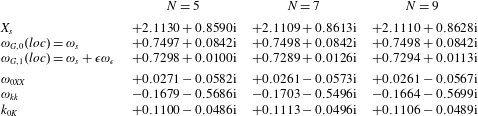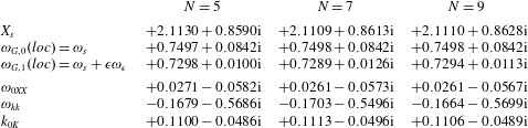For instance, the estimated values of $X_{s}$ and $\unicode[STIX]{x1D714}_{s}$ for a progressive increase of the polynomial order $N$ from $N=5$ to $N=9$ are reported in the first two rows of table 2. As it can be evinced from table 2, no significant discrepancies are shown by varying the order of the polynomial extrapolation in the considered range. Moreover, following the indications provided in Juniper & Pier (Reference Juniper and Pier2015), the numerical convergence in the estimation of $X_{s}$ and $\unicode[STIX]{x1D714}_{s}$ have been appraised by progressively including all points that satisfy the condition $\unicode[STIX]{x1D714}_{0,i}>\unicode[STIX]{x1D709}$ , varying $\unicode[STIX]{x1D709}$ from $0.1$ to $-0.1$ . This convergence test, whose results are not reported here for brevity, substantially confirmed that the values reported in table 2 are converged with a discrepancy which is less than 2 % for all the considered cases.

The position of the complex saddle point is found at $\unicode[STIX]{x1D714}_{s}=\unicode[STIX]{x1D714}_{G,0}(loc)=0.750+0.084\text{i}$ , $X_{s}=2.112+0.863\text{i}$ . These results are in agreement with Pier (Reference Pier2002), Juniper & Pier (Reference Juniper and Pier2015), as can be also evinced by table 1, thus validating the procedure and the numerical tools used for this study. The local approach predicts the global unstable eigenvalue with an error of $9.1\,\%$ . In this particular case, the error is larger for the complex part of the unstable eigenvalue, i.e. for the temporal growth factor. As a consequence, the standard local stability analysis estimates the critical Reynolds number $\mathit{Re}_{cr}\simeq 27.3$ , which differs significantly from the value determined by a global stability analysis, with a percentage error of about $42\,\%$ .

The results of the local stability analysis can be corrected as detailed in § 2.2. To do this, the coefficients in (2.10) have to be evaluated at the complex saddle point $X_{s}$ . To check the numerical convergence in the estimation of the mentioned coefficients and of $\unicode[STIX]{x1D714}_{G,1}(loc)$ , these quantities have been evaluated for increasing values of the order $N$ of the adopted rational function for continuation in the complex pane (see § 3 for details), and results, reported in table 2, demonstrate a substantial convergence.

Table 2.

Estimation of coefficients in (2.10) ( $\unicode[STIX]{x1D714}_{0XX}$ , $\unicode[STIX]{x1D714}_{kk}$ , $k_{0K}$ ) and of the complex global eigenvalues at different order of approximation ( $\unicode[STIX]{x1D714}_{G,0}(loc)$ , $\unicode[STIX]{x1D714}_{G,1}(loc)$ ) with increasing values of $N$ , i.e. the order of rational function used for continuation in the complex plane.

Applying (2.10), the resulting corrected eigenvalue is equal to $\unicode[STIX]{x1D714}_{G,1}(loc)=0.729+0.012\text{i}$ , demonstrating the efficacy of the correction which in this case decreases the error with respect to global stability analysis to approximately $3\,\%$ , as also reported in table 1. In particular, the accuracy of the predicted growth factor is greatly improved by the proposed correction, thus leading to an accurate estimation of $\mathit{Re}_{cr}$ , i.e. $\mathit{Re}_{cr}\simeq 45.2$ , which compares well with the true value, the discrepancy being of approximately $3.2\,\%$ .

Figure 2.

(a) Estimation of the $Re_{cr}$ for the primary wake instability of the flow past a circular cylinder. Green triangles: global stability analysis; red circles: local stability analysis not corrected; blue squares: local stability analysis with correction. Spatial position of the saddle point with $Re$ : real (b) and imaginary (c) part of $X_{s}$ , obtained considering a rational function of $N=7$ for continuation in the complex plane.

As a further assessment of the beneficial effects of the proposed correction, we report in figure 2(a) the values of the global growth rate estimated by the local stability analysis with and without correction, i.e. $\unicode[STIX]{x1D714}_{G,1}(loc)$ and $\unicode[STIX]{x1D714}_{G,0}(loc)$ respectively, in comparison with the equivalent values estimated by the global stability analysis, for values of Reynolds number ranging from $Re=25$ to $Re=75$ . The figure clearly shows that the applied correction systematically improves the predictions of the local stability analysis over the range of Reynolds numbers considered and, as already commented, significantly improves the prediction of the critical conditions for the onset of the wake instability. In addition, the position of the saddle point $X_{s}$ as a function of the Reynolds number is also reported in figure 2(b,c). Since the length of the recirculation region in the near wake of the cylinder increases with the flow Reynolds number, the saddle point moves slightly downstream, i.e. $\text{Re}(X_{s})$ increases. In contrast, the distance of $X_{s}$ from the real $X$ -axis, i.e. $\text{Im}(X_{s})$ , remains substantially unchanged, at least for the considered range of Reynolds numbers.

4.2 Flow past a wall-mounted hemispherical roughness element

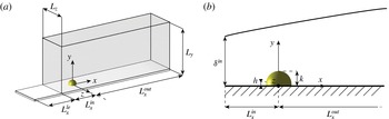
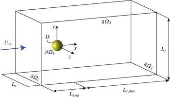
In this section we consider the three-dimensional flow over a wall-mounted roughness element which is positioned inside an incoming laminar boundary layer (BL). The considered configuration is sketched in figure 3(a,b) together with the considered Cartesian coordinate system. The roughness element is composed by a hemisphere of radius $R$ connected to the wall by a thin circular cylinder with the same radius and a height of $h=0.1R$ (for further geometrical details see Citro et al. Reference Citro, Giannetti, Luchini and Auteri2015). In this case, the Reynolds number, $Re_{k}$ , is based on the total height $k$ of the obstacle (see figure 3 b) and the flow velocity $U_{k}$ , i.e. the streamwise velocity that we would be measured at point ( $x=0$ , $y=k$ ) in the absence of the hemispherical obstacle. All quantities reported in the following in non-dimensional form are normalised using $k$ and $U_{k}$ as reference length and velocity. With reference to figure 3(a), the computational domain is characterised by $L_{x}^{in}=7R$ , $L_{x}^{out}=30R$ , $L_{y}=8R$ , $L_{z}=10R$ (labelled $M1$ in Citro et al. (Reference Citro, Giannetti, Luchini and Auteri2015)) and the inherent mesh has approximately $9\times 10^{3}$ spectral elements. Validation and convergence tests are reported in section 2D in Citro et al. (Reference Citro, Giannetti, Luchini and Auteri2015). Concerning the boundary conditions for the DNS, null velocity ( $\boldsymbol{u}=(0,0,0)$ ) is imposed at the solid boundaries, a fully developed Blasius BL velocity profile is imposed at the inlet of the domain and, finally, stress-free conditions, i.e. $p\boldsymbol{n}-Re^{-1}\unicode[STIX]{x1D735}\boldsymbol{u}\boldsymbol{\cdot }\boldsymbol{n}=0$ , are imposed on the remaining boundaries.

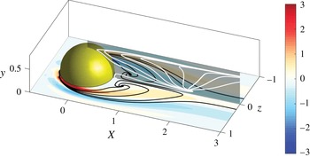
For this flow configuration, the results from the WKBJ at higher order are presented and compared with those obtained by the global analysis for $Re_{k}=450$ (see Citro et al. Reference Citro, Giannetti, Luchini and Auteri2015). The wall-normal vorticity and the velocity streamlines of the unstable base flow in the near wake of the roughness element are reported in figure 4. At this value of $Re_{k}$ , the flow is characterised by the shedding of periodic hairpin vortices inside the BL, with a Strouhal number $St=\unicode[STIX]{x1D714}k/2\unicode[STIX]{x03C0}U_{k}\simeq 0.16$ (for further details, see Citro et al. 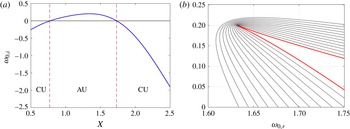Reference Citro, Giannetti, Luchini and Auteri2015). As reported in figure 5(a), the streamwise evolution of the absolute growth rate $\unicode[STIX]{x1D714}_{0,i}$ shows that the flow is absolutely unstable in the region $0.77<X<1.73$ . This is in reasonable agreement with the dimensions of the recirculation region in the near wake of the hemispherical element, that extends in streamwise direction up to $X=1.9$ (see figure 4).

Figure 3.

Flow past a wall-mounted hemispherical roughness: configuration and frame of reference (not in scale).

Following the same procedure detailed in § 4.1 for the circular cylinder, the saddle point is found for $\unicode[STIX]{x1D714}_{s}=\unicode[STIX]{x1D714}_{G,0}(loc)=1.6322+0.1994\text{i}$ and $X_{s}=1.2923-0.047\text{i}$ . For a further verification, the location ( $\unicode[STIX]{x1D714}_{s}$ , $X_{s}$ ) is found by a graphical method seeking the cusp point in the $\unicode[STIX]{x1D714}_{0}$ -plane. Referring to figure 5(b), the streamwise evolution of $\unicode[STIX]{x1D714}_{0}$ is plotted at different values of the imaginary part of the complex $X$ -plane, $X_{s,i}$ . The saddle point is then identified by the values for which a cusp formation is visible in the absolute frequency plane. The global analysis identifies, for this flow configuration, a reference complex eigenvalue equal to $\unicode[STIX]{x1D714}_{G}(glob)=1.858114+0.087148\text{i}$ (Citro et al. Reference Citro, Giannetti, Luchini and Auteri2015), which is slightly more stable than the one estimated by local analysis. However, the over-prediction of the global growth rate is a common characteristic of the local analysis, as already highlighted, for example, in Juniper et al. (Reference Juniper, Tammisola and Lundell2011). Lastly, the correction in (2.10) is considered in order to obtain a more accurate estimate of the global eigenvalue, taking into account the correction term $\unicode[STIX]{x1D714}_{\unicode[STIX]{x1D716}}$ in the WKBJ expansion at order $O(\unicode[STIX]{x1D716}^{1})$ . In particular, following the same extrapolation procedure used for the circular cylinder flow configuration presented in § 4.1, the resulting complex global frequency is found equal to $\unicode[STIX]{x1D714}_{G,1}(loc)=1.6781+0.0376\text{i}$ . This result shows that, for this specific case, the correction procedure leads to an improved estimation of the global eigenvalue, especially of its imaginary part, which is related to the frequency in time of the global mode. For the sake of completeness, the correction coefficients in (2.10), using $N=7$ as the order of the rational function, are: $\unicode[STIX]{x1D714}_{0XX}=1.8418-1.6684\text{i}$ , $\unicode[STIX]{x1D714}_{kk}=0.0235-0.0715\text{i}$ , $k_{0K}=1.6445-1.0907\text{i}$ .

Figure 4.

Streamlines of the flow past the hemispherical roughness element at $Re_{k}=450$ in the planes $y=0.03$ and $z=0$ . Colour contours depict the wall-normal vorticity in the plane $y=0.03$ .

Figure 5.

(a) Spatial evolution of the absolute growth rate $\unicode[STIX]{x1D714}_{0i}$ (CU $=$ convectively unstable flow, AU $=$ absolutely unstable flow); (b) evolution of $\unicode[STIX]{x1D714}_{0}$ for different values of the complex $X$ obtained with a seventh-order rational function for continuation in the complex plane. The red line corresponds to the saddle-point value, $\text{Im}(X)=-0.047$ and the successive lines are evaluated at different values of $\text{Im}(X)$ , with steps equal to $-0.009$ .

4.3 Flow past a fixed sphere

In this section, we detail the numerical results obtained for a sphere of radius $R$ positioned in a uniform incompressible flow. Figure 6 depicts the flow configuration and the frame of reference adopted in the present study. The reference quantities for the normalisation of the flow quantities and for the definition of the flow Reynolds number, $\mathit{Re}_{D}$ , are the sphere diameter $D$ and the uniform streamwise velocity $U_{\infty }$ . The same flow configuration has been characterised by DNS and global stability analysis in Citro et al. (Reference Citro, Tchoufag, Fabre, Giannetti and Luchini2016) and we use here the same computational domain and discretisation parameters adopted in that paper. With reference to figure 6, the dimensions of the computational domain used for both the simulation and the global stability analysis are: $L_{x,up}=12$ , $L_{x,dwn}=35$ , $L_{y}=24$ , $L_{z}=24$ ; the mesh is made by approximately $1.3\times 10^{4}$ spectral elements of degree $N_{p}=13$ . On both the inlet boundary $\unicode[STIX]{x2202}\unicode[STIX]{x1D6FA}_{1}$ and the lateral boundaries $\unicode[STIX]{x2202}\unicode[STIX]{x1D6FA}_{3}$ a constant velocity profile is imposed, which is parallel to the $x$ axis, and a stress-free condition is imposed on the outlet boundary $\unicode[STIX]{x2202}\unicode[STIX]{x1D6FA}_{2}$ . Validation and convergence tests leading to the adopted choice of the numerical discretisation are detailed in Citro et al. (Reference Citro, Tchoufag, Fabre, Giannetti and Luchini2016). Here we focus our attention on the occurrence of the second bifurcation that arises at $\mathit{Re}_{D}=271.8$ , which leads the flow from a steady asymmetric state to a flow configuration characterised by an asymmetric mean flow and by the time-periodic shedding of vortical structures in the wake. For $\mathit{Re}_{D}=275$ the vortex shedding frequency in terms of the Strouhal number is equal to $St\simeq (\unicode[STIX]{x1D714}D/2\unicode[STIX]{x03C0}U_{\infty })\simeq 0.13$ . 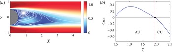An example of the steady unstable flow past the sphere in supercritical conditions is given in figure 7(a), where the modulus of the velocity field and the velocity streamlines are shown for the section $z=0$ (the mid-plane of the computational domain) at $\mathit{Re}_{D}=275$ .

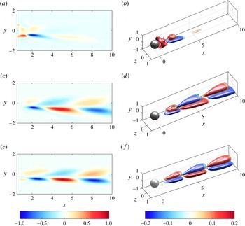
When the global stability analysis is applied to the flow field in figure 7(a), a globally unstable mode is found with an associated complex eigenvalue equal to $\unicode[STIX]{x1D714}_{G}(glob)\simeq 0.8092+0.006\text{i}$ . The real part of the corresponding global eigenmode is plotted in figure 9(e,f).

Figure 6.

Flow past a spherical body: configuration and frame of reference (not to scale).

When the classical local stability analysis is applied to the wake, i.e. considering only first-order terms in the WKBJ expansion, a region of absolute instability is identified by inspecting where the absolute growth rate $\unicode[STIX]{x1D714}_{0,i}$ is positive. As shown in figure 7(b), where the streamwise evolution of $\unicode[STIX]{x1D714}_{0,i}$ is depicted, the flow is absolutely unstable in the region $0.47<X<1.95$ . The length of this region is comparable to that of the asymmetric recirculation bubble, which extends in the streamwise direction from the top of the sphere, where separation first occurs, to $X\simeq 2$ (see figure 7 a).

Figure 7.

(a) Modulus of velocity (colour) and streamlines of the flow past a sphere at $\mathit{Re}_{D}=275$ in the midplane ( $z=0.0$ ); (b) spatial evolution of the absolute growth rate $\unicode[STIX]{x1D714}_{0,i}$ (CU  $=$  convectively unstable flow, AU  $=$  absolutely unstable flow).

As described in § 2.2, continuing $\unicode[STIX]{x1D714}_{0}(X)$ in the complex $X$ plane, the eigenvalue of the globally unstable flow can be approximated at the leading order $\unicode[STIX]{x1D716}$ by the eigenvalue estimated at the saddle point ( $\unicode[STIX]{x1D714}_{s}$ , $X_{s}$ ). The numerical procedure for continuation in the complex plane, already commented on in the previous sections, makes it possible to identify the saddle point at $\unicode[STIX]{x1D714}_{s}=\unicode[STIX]{x1D714}_{G,0}(loc)=0.7369+0.2235\text{i}$ and $X_{s}=1.3394+0.2397\text{i}$ . 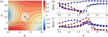This is shown in figure 8(a), where $\unicode[STIX]{x1D714}_{0,i}$ is plotted in the complex $X$ plane. As in the case of the circular cylinder, the error (compared to the reference quantity $\unicode[STIX]{x1D714}_{G}(glob)\simeq 0.8092+0.006\text{i}$ ) affects both the frequency of the global mode and, more severely, the growth rate (i.e. the imaginary part of $\unicode[STIX]{x1D714}$ ), which is overestimated by a factor approximately equal to $37.25$ . Globally, the relative error on the eigenvalue is approximately equal to $29\,\%$ .

Figure 8.

(a) Distribution of $\unicode[STIX]{x1D714}_{0,i}$ in the complex $X$ plane. Streamwise evolution of the imaginary (b) and real (c) parts of the complex local wavenumbers $k^{+}$ (blue lines) and $k^{-}$ (red lines) obtained by the local dispersion relation with $\unicode[STIX]{x1D714}=\unicode[STIX]{x1D714}_{G,0}(loc)$ (●), $\unicode[STIX]{x1D714}=\unicode[STIX]{x1D714}_{G,1}(loc)$ (▪) and $\unicode[STIX]{x1D714}=\unicode[STIX]{x1D714}_{G}(glob)$ (▾), respectively.

Figure 9.

Real part of the leading direct global mode calculated using the standard (uncorrected) local analysis (a,b), the corrected local approach (c,d) and the global stability analysis (e,f). (a,c,e) Contour plot of the streamwise velocity component $\hat{u}$ in the plane ( $z=0.0$ ). (b,d,f) Perspective view of the corresponding isocontours.

The estimated global complex eigenvalue is then used in the local dispersion relation at different streamwise sections to evaluate the local shape of the associated global eigenmode. In this way, from (2.8) and following the indications provided by Juniper & Pier (Reference Juniper and Pier2015), the direct mode can be reconstructed by local analysis. As a first step the spatial evolution of the complex wavenumbers $k^{\mp }$ and the corresponding local spatial eigenmode is evaluated considering the saddle-point complex frequency $\unicode[STIX]{x1D714}_{G,0(loc)}$ in the dispersion relation. This has been done by considering $X$ -sections uniformly placed downstream the sphere with a spacing equal to $\unicode[STIX]{x0394}X=0.025$ . The streamwise evolution of the wavenumbers $k^{\mp }$ is shown in figure 8(b,c) with circular symbols. Starting from this result the structure of the global eigenmode is estimated using (2.8). Figure 9(a,b) shows the resulting spatial evolution of the velocity streamwise component of the unstable eigenmode reconstructed as described above. As can be deduced from figure 9, the standard local analysis (WKBJ at $O(\unicode[STIX]{x1D716}^{0})$ , as in Juniper et al. (Reference Juniper, Tammisola and Lundell2011)) provides a poor reconstruction of the direct mode. Indeed, the structure of the direct mode, obtained by the standard local analysis and depicted in figure 9(a,b), is very different from the reference one obtained by global stability analysis and depicted in figure 9(e,f).

In order to highlight the beneficial effects that can be obtained by the proposed correction, the local analysis is now repeated for the same flow including the higher-order terms in the WKBJ expansion (WKBJ at $O(\unicode[STIX]{x1D716}^{1})$ ). As a first result the corrected global eigenvalue is now equal to $\unicode[STIX]{x1D714}_{G,1(loc)}=0.7898+0.0266\text{i}$ . The percentage error with respect to the reference value obtained by global stability analysis is now reduced to $4\,\%$ ; it was approximately equal to $29\,\%$ without including higher-order terms. For sake of completeness we also provide the coefficients used in (2.10) so as to estimate the global eigenvalue with the higher-order correction: $\unicode[STIX]{x1D714}_{0XX}=0.7042-0.1965\text{i}$ , $\unicode[STIX]{x1D714}_{kk}=-0.1334-0.3333\text{i}$ and $k_{0X}=0.9252+0.6703\text{i}$ .

The present test case has also been used to appreciate the importance of retaining the non-parallel terms containing $V_{b}$ and $W_{b}$ and $\unicode[STIX]{x2202}U_{b}/\unicode[STIX]{x2202}X$ in the estimation of the corrected frequency $\unicode[STIX]{x1D714}_{G,1}(loc)$ . As discussed in § 2.2, the inclusion of the mentioned terms is equivalent to the explicit inclusion of the term $\unicode[STIX]{x1D6FF}\unicode[STIX]{x1D714}$ appearing in Huerre & Monkewitz (Reference Huerre and Monkewitz1990) (see equation (6.1) of the cited reference) in the estimation of $\unicode[STIX]{x1D714}_{G,1}(loc)$ . In our case the term $\unicode[STIX]{x1D6FF}\unicode[STIX]{x1D714}$ is evaluated by subtracting the value of $\unicode[STIX]{x1D714}_{G,1}(loc)$ obtained by alternately including and neglecting the mentioned non-parallel terms in (2.5). As a result, it is found that $\unicode[STIX]{x1D6FF}\unicode[STIX]{x1D714}\approx 0.1963+0.0829i$ , which is not negligible if compared with the estimated global eigenvalue $\unicode[STIX]{x1D714}_{G,1(loc)}=0.7898+0.0266\text{i}$ .

Besides the error reduction in the estimation of the global eigenvalue, the proposed correction can also lead to a significant improvement in the estimation of the spatial shape of the corresponding eigenmode. In particular, as remarked above, a solution which is accurate up to order $O(\unicode[STIX]{x1D716})$ can be obtained by determining the slowly evolving function $A(X)$ and by computing the global mode shape with the corrected eigenvalue $\unicode[STIX]{x1D714}_{G,1(loc)}$ , as expressed in the following, using the same conventions and notation proposed in Juniper et al. (Reference Juniper, Tammisola and Lundell2011):

(4.1) $$\begin{eqnarray}\hat{\boldsymbol{q}}(x,y,z)\sim A(X)^{\mp }\hat{\boldsymbol{q}}(y,z;X)\exp \left[\text{i}\unicode[STIX]{x1D716}^{-1}\int _{X_{s}}^{X}k^{\mp }(\unicode[STIX]{x1D714}_{G,1}(loc);X^{\prime })\,\text{d}X^{\prime }\right],\end{eqnarray}$$

where the local wavenumbers $k^{\mp }$ are now evaluated considering $\unicode[STIX]{x1D714}_{G,1}(loc)$ in the dispersion relation. Their resulting streamwise evolution is depicted in figure 8(b,c) using square symbols. For comparison, in the same figures we report the same branches $k^{\mp }$ evaluated by forcing $\unicode[STIX]{x1D714}_{G}(glob)$ in the dispersion relation (with triangle symbols) and evaluated by forcing $\unicode[STIX]{x1D714}_{G,0}$ (circular symbols). For the sphere case, a marked improvement is already obtained by just recomputing the eigenfunction shape, using the corrected frequency $\unicode[STIX]{x1D714}_{G,1}(loc)$ in the dispersion relation and without including the slow amplitude function $A(X)$ . With this aim, figure 9(c,d) shows the spatial distribution of the streamwise velocity component of the unstable mode retrieved using the corrected eigenvalue $\unicode[STIX]{x1D714}_{G,1}(loc)$ . As can be deduced from figure 9, the mode obtained using the present approach is in excellent agreement with the corresponding mode shape obtained through a fully three-dimensional global stability analysis, reported in figure 9(e,f). Note that, in a linear setting, the amplitude of the mode is undetermined, so that a normalisation must be chosen when comparing the eigenfunctions: here we used $\text{max}|\hat{u} (x,y,z)|=1$ , while the phase was fixed at a given position in space. A further improved reconstruction, accurate up to $O(\unicode[STIX]{x1D716}^{1})$ , could be obtained by using the corrected frequency $\unicode[STIX]{x1D714}_{G,1}(loc)$ not only to evaluate the eigenfunction shape but also to evaluate the slow amplitude function $A(X)$ appearing in expression (2.8). This can be achieved by writing the solvability condition of the outer problem at order $O(\unicode[STIX]{x1D716}^{1})$ : for details on the derivation and practical implementation of the solvability condition we refer the interested reader to Zuccher & Luchini (Reference Zuccher and Luchini2014) and Giannetti & Luchini (Reference Giannetti and Luchini2006): the resulting linear differential equation for $A(X)$ can be readily solved to provide, together with (4.1), an approximation of the eigenmode which is accurate up to $O(\unicode[STIX]{x1D716}^{1})$ . Here we did not evaluate the amplitude $A(X)$ , since in this case the correction can expected to be very small (not appreciable from a graphical point of view) and the reconstruction based on the corrected frequency $\unicode[STIX]{x1D714}_{G,1}(loc)$ already provides excellent results.