





Impact Statement
Salt concentration gradients generated by merging electrolyte streams at the junction of a microfluidic device can drive the motion of colloids through diffusiophoresis and fluid motion along solid boundaries via diffusioosmosis. Such junction microdevices have been adopted for particle separation, focusing and characterisation, yet most studies have examined the dynamics only near the junction. Here, we employ a junction device with a long downstream channel to observe the particle dynamics over time scales comparable to the characteristic time for the diffusion-driven mixing of the electrolyte streams. Experiments and theory reveal that the particle dynamics depends strongly on their position within the channel because of the coupling between the hydrodynamics, wall diffusioosmosis and particle diffusiophoresis, as well as the dependence of diffusioosmosis and diffusiophoretic mobility on the local salt concentration. Depending on these factors, particles exhibit diffusive, sub-diffusive or reverse motion along the sideways direction perpendicular to the background flow. By linking the particles’ dynamics to their properties, we propose microfluidic approaches for determining particle diffusiophoretic mobility, size and zeta potential. These findings will support the design of microfluidic platforms for the passive (i.e. without external fields) and continuous concentration, separation and characterisation of charged colloids using portable, easy-to-use devices with potential for bioanalytical, biomedical and environmental applications.
1. Introduction
When a solute concentration gradient is established on a solid surface and the solute interacts with the surface via an interaction potential, an osmotic pressure gradient arises at the liquid interfacial layer near the surface where the solute–surface interactions occur. As a result, the liquid sets into motion so that the osmotic pressure gradient is balanced by the liquid viscous stress on the surface. This transport mechanism is called diffusioosmosis and, at a scale length much larger than the interfacial layer thickness, it appears as a liquid slip or diffusioosmotic velocity
 ${u}_{\text{DO}}$
at the solid surface (Anderson Reference Anderson1989; Marbach & Bocquet Reference Marbach and Bocquet2019). For a neutral solute interacting with an uncharged surface via the steric effect,
 ${u}_{\text{DO}}$
is proportional to the solute concentration gradient
 $\nabla c$
. For a charged surface exposed to a salt concentration gradient, the ions and the surface interact via an electrostatic potential within the electric double layer (EDL) – a diffuse region near the surface that is enriched in counterions and depleted of coions (Hunter Reference Hunter2001). In this case, the diffusioosmotic velocity is proportional to
 $\nabla \log c$
. Furthermore, if counterions and coions have different diffusivities, a bulk electric field builds up spontaneously under the salt concentration gradient – provided that no bulk current exists – and an extra electroosmotic contribution, also proportional to
 $\nabla \log c$
, adds to the diffusioosmotic effect. For electrolyte diffusioosmosis, the osmotic pressure and electric field contributions are often referred as chemiosmosis and electroosmosis, respectively, and the overall coefficient of proportionality
 ${\Gamma _{\mathrm{DO}}}=-{u}_{\text{DO}}/\nabla \log c$
is called the diffusioosmotic mobility. On the other hand, when a charged colloid is exposed to a salt concentration gradient, a diffusioosmotic slip velocity arises at the particle surface, leading to the spontaneous migration of the particle in the opposite direction – an effect known as diffusiophoresis. As for electrolyte diffusioosmosis, the diffusiophoresis velocity
 ${u}_{\tiny {\text{DP}}}$
of a colloidal particle within a salt concentration gradient is proportional to
 $\nabla \log c$
with
 ${\Gamma _{\mathrm{DP}}}={u}_{\tiny {\text{DP}}}/\nabla \log c$
the diffusiophoretic mobility.
In the last two decades, microfluidics has catalysed a surge of interest in diffusiophoresis and diffusioosmosis (Ault & Shin Reference Ault and Shin2025; Shin Reference Shin, Ault, Toda-Peters and Shen2020, Reference Shim2022). This is because microfluidic systems have allowed researchers to investigate the liquid and colloid dynamics at the length and time scales characteristic of diffusiophoresis and diffusioosmosis transport (Abécassis et al. Reference Abécassis, Cottin-Bizonne, Ybert, Ajdari and Bocquet2008; Kar et al. Reference Kar, Chiang, Ortiz Rivera, Sen and Velegol2015; Shin et al. Reference Shin, Um, Sabass, Ault, Rahimi, Warren and Stone2016). Merging stream channel geometries, provided by T-, Y- and
 $\Psi$
-shaped junction devices, have been widely adopted to generate steady-state salt concentration gradients (Abécassis et al. Reference Abécassis, Cottin-Bizonne, Ybert, Ajdari and Bocquet2008; Collins et al. Reference Collins, Mohajerani, Ghosh, Guha, Lee, Butler, Sen and Velegol2019; Fillbrook et al. Reference Fillbrook, Middleton, Rashidnejad, Sapre, Schmidt, Sen and Beves2025; Möller et al. Reference Möller, Kriegel, Kieß, Sojo and Braun2017; Seo et al. Reference Seo, Park, Lee, Lee and Kim2020; Shimokusu et al. Reference Shimokusu, Maybruck, Ault and Shin2019; Shin et al. Reference Shin, Ault, Warren and Stone2017; Shin et al. Reference Shin, Ault, Toda-Peters and Shen2020; Singh et al. Reference Singh, Vladisavljević, Nadal, Cottin-Bizonne, Pirat and Bolognesi2020; Timmerhuis & Lammertink Reference Timmerhuis and Lammertink2022; Visan & Lammertink Reference Visan and Lammertink2019; Yang et al. Reference Yang, McKenzie, Yi, Khair, Garoff and Tilton2023, Reference Yang, McKenzie, Pavlat, Johnson, Khair, Garoff and Tilton2024). In those devices, the main direction of the concentration gradient is perpendicular to the flow and parallel to the channel width-wise direction. Many studies have focussed on the solute-driven migration of colloids along this transverse direction and applied it for the validation of theoretical frameworks (Collins et al. Reference Collins, Mohajerani, Ghosh, Guha, Lee, Butler, Sen and Velegol2019; Timmerhuis & Lammertink Reference Timmerhuis and Lammertink2022; Yang et al. Reference Yang, McKenzie, Pavlat, Johnson, Khair, Garoff and Tilton2024) and for applications such as particle focusing (Abécassis et al. Reference Abécassis, Cottin-Bizonne, Ybert, Ajdari and Bocquet2008; Shin et al. Reference Shin, Ault, Warren and Stone2017; Shin Reference Shin, Ault, Toda-Peters and Shen2020) and separation (Seo et al. Reference Seo, Park, Lee, Lee and Kim2020; Shimokusu et al. Reference Shimokusu, Maybruck, Ault and Shin2019). These studies delve with the dynamics of colloidal particles in the bulk and away from the channel walls, hence particle diffusiophoresis is the main transport mechanism meanwhile wall diffusioosmosis is either weak or entirely negligible.
In Singh et al. (Reference Singh, Vladisavljević, Nadal, Cottin-Bizonne, Pirat and Bolognesi2020), we showed how the Poiseuille-like velocity profile in a
 $\Psi$
-junction device generates also an additional vertical component of the salt concentration gradient, and thus of the particle diffusiophoresis velocity, perpendicular to the flow and parallel to the depth-wise direction of the channel. This component drives the accumulation of particles at the top and bottom walls of the microfluidic devices, typically made of glass or polydimethylsiloxane (PDMS). Near these charged solid surfaces, the dynamics of the accumulated particles is governed by the balance between the opposite effects of wall diffusioosmotic flows and particle diffusiophoresis (Chakra et al. Reference Chakra, Singh, Vladisavljević, Nadal, Cottin-Bizonne, Pirat and Bolognesi2023; Liu & Pahlavan Reference Liu and Pahlavan2025; Migacz, Durey, & Ault Reference Migacz, Durey and Ault2023). Our group has exploited this effect and designed a double
 $\Psi$
-junction device to characterise the size of polymer beads with similar zeta potentials or the zeta potential and lipid composition of charged liposomes with similar sizes (Chakra et al. Reference Chakra, Singh, Vladisavljević, Nadal, Cottin-Bizonne, Pirat and Bolognesi2023). The same device was also adopted for the size-based separation of polymer beads (Chakra et al. Reference Chakra, Singh, Vladisavljević, Nadal, Cottin-Bizonne, Pirat and Bolognesi2023) and, by leveraging the EDL polarisation effect, for the separation of polymer beads based on the surface concentration of a charged group (Chakra et al. Reference Chakra, Puijk, Vladisavljević, Cottin-Bizonne, Pirat and Bolognesi2025). Most of the studies on the dynamics in junction devices accounting for interwoven effects of particle diffusiophoresis and wall diffusioosmosis have been limited to short channel devices, where the relaxation time of the solute concentration gradient is much larger than the particle average residence time in the device. Migacz, Durey, and Ault (Reference Migacz, Durey and Ault2023) adopted a longer channel so that the particle dynamics was monitored on a time scale comparable to the mixing time of the electrolyte solutions. However, in that study the focus was on particle dynamics near the channel walls and not in the bulk.
Here, we explore the three dimensional salt-driven dynamics of carboxyl-modified polystyrene particles of varying sizes and zeta potentials located in the bulk and near the walls of a double
 $\Psi$
-junction devices with long channels, for which the particle average residence time is of the same order as the salt gradient relaxation time. First, we discuss the dependence of particle and wall zeta potentials on the local salt concentration and show how EDL polarisation affects the calculation of particle diffusiophoretic mobility – an effect neglected in previous experimental studies. We then consider the dynamics of particles either located in the bulk, away from the boundaries or accumulated near the top and bottom walls. In the bulk, the effects of particle diffusiophoresis and wall diffusioosmosis are additive, whereas, near the walls, these effects are competitive. Through analytical calculations and experimental validation, we rationalise the observed behaviours and suggest a microfluidic method to quantify particle diffusiophoretic mobility. Finally, we propose a microfluidic strategy for determining the size or zeta potential of particles with varying diameters and zeta potentials, provided that one of these two properties is already known a priori. Our findings will be useful for the design of junction microfluidic devices for the salt-driven accumulation, separation and characterisation of colloidal particles, such as macromolecules (Friedrich et al. Reference Friedrich, Burke, Liu, Ivory and Wang2017; Lechlitner & Annunziata Reference Lechlitner and Annunziata2018; Palacci et al. Reference Palacci, Abécassis, Cottin-Bizonne, Ybert and Bocquet2010), nano- and micro-beads, liposomes and cells (Hartman, Božic, & Derganc Reference Hartman, Božič and Derganc2018; Rasmussen, Pedersen, & Marie Reference Rasmussen, Pedersen and Marie2020) in continuous flow settings.
2. Materials and methods
2.1. Materials
The PDMS RTV-615a and curing agent RTV-615b used for the fabrication of microfluidic channels were purchased from Techsil, UK. Pre-cleaned Corning™ glass slides used as the substrate to make PDMS microfluidic chips were purchased from Thermo Fisher Scientific. Silicon wafers used to make masters for PDMS devices were purchased from Inseto Limited, UK. The SU-8 2050 used for the fabrication of replica moulds was purchased from A-Gas, UK. Masks for replica mould fabrication were designed in house and printed by Micro Lithography services Ltd. (Chelmsford, UK). The 1H, 1H, 2H, 2H-Perfluorooctyl-trichlorosilane was purchased from Merck and used for the salinisation of the SU-8 masters. All aqueous solutions were prepared using deionised water produced from a Thermo Fisher Smart2Pure purification system (Thermo Fisher Scientific, USA). Lithium chloride salt (LiCl, 99 %) used to make the electrolyte solutions, was purchased from Acros Organics. Red fluorescent (580/605), carboxyl-modified nano-beads (Invitrogen™), used to make colloidal suspensions, were purchased from Thermo Fisher Scientific. Particles of nominal diameters 0.1, 0.2, 0.5 and 1
 $\mu$
m were part of a size kit with lot number 2294999, referred to in this manuscript as lot A. Additionally, particles of nominal size 0.2
 $\mu$
m with lot number 1934417A, referred to as lot B, and of nominal size 1
 $\mu$
m with lot number 2770870, referred to as lot C, were also used.
2.2. Sample preparation
For all microfluidic experiments, the colloidal particle stock dispersions (2
 $\%$
solids) were diluted in
 $0.1\,$
mM LiCl solution. All colloidal dispersions with sub-micron particles were prepared at 0.02% v/v particle concentration. For the dispersions with 1
 $\mu$
m colloids, a particle concentration of 0.002% v/v was used. For all particle characterisation experiments, the particle stock dispersion were diluted in LiCl solution of varying salt concentrations. The particle concentrations of the diluted dispersions were kept identical to those used for the microfluidic experiments (
 $0.02\%$
v/v and
 $0.002\%$
v/v for sub-micron particles and
 $1\,\mu$
m particles, respectively).
2.3. Fabrication and operation of the microfluidic devices
Microfluidic devices were made from PDMS channels bonded to a glass microscope slide via oxygen plasma treatment. To make the PDMS channels, standard photo-lithography and soft-lithography techniques were employed. A home-made inverted optical microscope was used to capture epi-fluorescence micrographs of the device. The microscope was assembled with Thorlabs components, with an X-Cite 200 fluorescent lamp to excite the sample (Excelitas, Canada) and a CCD camera (Ximea MQ013MG-ON) for capturing images. A Nikon Plan fluor 10x objective lens (0.30 NA) was used for online imaging of the particle dynamics inside the microfluidic devices. A red fluorescent filter set, purchased from ThorLabs Inc., USA, consisting of an excitation (559 nm
 $\pm$
12 nm), emission (630 nm
 $\pm$
35 nm) and dichroic filters (533–580 nm reflection band), was used to image red fluorescent colloids. All epi-fluorescence micrographs of the microfluidic devices were acquired by positioning the focal plane nearby the bottom (glass) wall of the channel. No difference was observed when the focal plane was located near the top (PDMS) wall or mid-way through the channel depth.
2.4. Sample characterisation
Colloid samples were characterised by dynamic light scattering and electrophoretic light scattering, using a Zetasizer Ultra (Malvern Panalytical). For size measurements, non-invasive backscatter (173
 $^\circ$
detection angle) was used for all particle sizes. Error bars for particle size and zeta potential were calculated as one standard deviation of at least three consecutive measurements of the sample loaded in the Zetasizer. The zeta potential for each particle type was measured across a range of LiCl concentration. The pH of the solutions, without particles, was measured using a Mettler Toledo Five Easy pH meter.
3. Results
A double
 $\Psi$
-junction device, schematically shown in figure 1a, was used to generate a steady-state salt concentration gradient and induce particle focusing. At the narrower upstream junction, the inner inlet channel, fed with a LiCl solution of low concentration (
 $c_{\scriptscriptstyle L}=0.1\,$
mM), meets the middle inlet streams made of a colloidal dispersion of red fluorescent carboxyl-modified polystyrene particles and LiCl at concentration
 $c_{\scriptscriptstyle L}$
. The inner and middle inlet channels merge into the middle channel of width
 $w_m$
. At the wider downstream junction, the middle channel meets the outer inlet channels, fed with a LiCl solution of high concentration (
 $c_{\scriptscriptstyle H}=10\,$
mM), and merges into the main channel of width
 $w$
. The length of the main channel is
 $L=36\,$
mm, allowing for the monitoring of the particle dynamics over an extended particle average residence time,
 $t_{res}=L/U=2.6\,s$
, with
 $U$
the average flow velocity. The dashed lines in figure 1a represent the outer boundaries of the colloidal streams, here also referred to as colloidal bands. A reference coordinate system is introduced, with the
 $z$
axis parallel to the direction of the main flow, the
 $x$
axis parallel to the channel width-wise direction and the
 $y$
axis parallel to the channel depth-wise direction. The origin of the reference system is located at the downstream junction and at the mid-point along the channel depth and width. The flow rates of the inner, middle and outer streams were fixed to
 $3.6\,\mu$
L min
 $^{-1}$
. All channels have a depth of
 $h=45\,\mu$
m. The widths of the inner inlet, middle and main channels are 100, 200,
 $300\,\mu$
m, respectively, whereas the widths of the middle and outer inlet channels are
 $50\,\mu$
m. Consequently, the average flow velocity,
 $U=13.3\,$
mm s
 $^{-1}$
, is the same in all channels. Note that, in contrast to the single-junction configuration, the double-junction geometry minimises the overlap between the fluorescence signals of colloids located in the bulk and those near the surfaces (Chakra et al. Reference Chakra, Singh, Vladisavljević, Nadal, Cottin-Bizonne, Pirat and Bolognesi2023). Consequently, the dynamics of the particles at these two locations along the channel depth can be investigated using an epi-fluorescence microscope rather than a more complex confocal microscopy system.
(a) Schematic of the double-junction device for the manipulation and focusing of carboxyl-modified polystyrene particles, shown as red dots, using a salt concentration gradient.
 $w_m=200\,\mu$
m and
 $w=300\,\mu$
m. (b) Sequence of epi-fluorescence micrographs taken at increasing distances from the downstream junction, ranging from
 $z/w_m$
= 5 to 170. Particles are from the
 $0.2\,\mu$
m (lot A) sample with
 $\zeta =-39.0\pm 0.2\,$
mV at
 $0.1\,$
mM LiCl. Scale bar represents 50
 $\mu m$
.

Figure 1 Long description
Panel (a) Schematic of the double-junction device for the manipulation and focusing of carboxyl-modified polystyrene particles, shown as red dots, using a salt concentration gradient. wm = 200 μm and w =300 μm. Panel (b) Sequence of epi-fluorescence micrographs taken at increasing distances from the downstream junction,ranging from z/wm =5 to 170. Particles are from the 0.2 μm (lotA) sample with ζ=−39.0 ±0.2 mV at 0.1 mM LiCl. Scalebar represents 50 μm.
Particles exhibit distinctly different behaviours depending on the presence or absence of a salt concentration gradient. In the control experiments (i.e. without a salt concentration gradient), a LiCl solution of low concentration
 $c_{\scriptscriptstyle L}$
is injected into the outer inlet channels (figure S1). Under these conditions, colloids remain homogeneously dispersed in the colloidal bands and exhibit minimal transversal migration, inasmuch as the distances between the outer edges of the colloidal bands, termed
 $\Delta w_0$
, increase slightly across the length of the microfluidic device due to colloid diffusion (figure S1).
The typical dynamics of sub-micron beads in presence of a salt concentration gradient is illustrated in figure 1b by the sequence of epi-fluorescence micrographs taken at various distances along the device, ranging from
 $z/w_m=5$
(i.e.,
 $z=1\,$
mm) to 170 (i.e.,
 $z=34\,$
mm), for
 $0.2\,\mu$
m (lot A) particles. As previously reported by Abécassis et al. (Reference Abécassis, Cottin-Bizonne, Ybert, Ajdari and Bocquet2008), the component of the salt concentration gradient in the channel width-wise direction,
 $\partial _x c$
, leads to the widening of the distance
 $\Delta w$
between the outer edges of the colloidal bands due to the particle’s diffusiophoresis velocity
 $u_{{\mathrm{\tiny{DP}}}_x} = {\Gamma _{\mathrm{DP}}} \, \partial _x \ln c$
, with
 ${\Gamma _{\mathrm{DP}}} \gt 0$
. Simultaneously, a component of the salt concentration gradient in the channel depth-wise direction,
 $\partial _y c$
, arises because of the Poiseuille-like flow velocity profile (Singh et al. Reference Singh, Vladisavljević, Nadal, Cottin-Bizonne, Pirat and Bolognesi2020). Specifically, in the mid-depth region of the channel and away from the channel walls, the shear rate
 $\partial _y u_z$
is negligible and the width
 $\delta _c(y\simeq 0,z)$
of the transition zone between the low and high salt concentration streams scales as
 $\delta _c(y\simeq 0,z)\propto z^{1/2}$
. Conversely, in the regions close to the top and bottom walls, the shear rate
 $\partial _y u_z\simeq 3\,U/h$
affects the salt diffusion transport rate, leading to a different scaling for the transition zone width,
 $\delta _c(y\to \pm h/2,z)\propto z^{1/3}$
for
 $z\ll U\,h^2/D_c$
(Salmon & Ajdari Reference Salmon and Ajdari2007). Here,
 $D_c$
is the ambipolar salt diffusivity calculated as
 $D_c = 2 D_p D_n / (D_p + D_n)$
, where
 $D_p=1.026\times 10^{-9}\,$
m
 $^2$
s
 $^{-1}$
is the diffusivity of the cation, Li
 $^+$
, at 25
 $^\circ$
C (Mills Reference Mills1957) and
 $D_n=1.964\times 10^{-9}\,$
m
 $^2$
s
 $^{-1}$
is the diffusivity of the anion, Cl
 $^-$
, at 25
 $^\circ$
C (Tanaka & Nomura Reference Tanaka and Nomura1987), leading to
 $D_c=1.348\times 10^{-9}\,$
m
 $^2$
s
 $^{-1}$
. The resulting inhomogeneous salt distribution along the channel depth generates a vertical component of the particle’s diffusiophoretic velocity,
 $u_{{\mathrm{\tiny{DP}}}_y} = {\Gamma _{\mathrm{DP}}} \, \partial _y \ln c$
, which drives the colloids from the bulk towards the top and bottom walls and induces their accumulation at two symmetric focusing regions (figure S2) (Chakra et al. Reference Chakra, Singh, Vladisavljević, Nadal, Cottin-Bizonne, Pirat and Bolognesi2023; Liu & Pahlavan Reference Liu and Pahlavan2025; Migacz, Durey, & Ault Reference Migacz, Durey and Ault2023; Singh et al. Reference Singh, Vladisavljević, Nadal, Cottin-Bizonne, Pirat and Bolognesi2020). In the epi-fluorescence micrographs in figure 1b, these regions appear as two accumulation peaks separated by a distance
 $\Delta _p(z)$
. As we demonstrated in Chakra et al. (Reference Chakra, Singh, Vladisavljević, Nadal, Cottin-Bizonne, Pirat and Bolognesi2023) using confocal microscopy analysis, a pair of symmetric accumulation peaks forms both at the top and the bottom wall of the device. However, in epi-fluorescence imaging the top and bottom peaks overlap and only two, instead of four, accumulation peaks are visible in the epi-fluorescence micrographs. It is worth noting that the vertical component of the particle diffusiophoretic velocity,
 $u_{{\mathrm{\tiny{DP}}}_y}$
, vanishes for
 $z\gg U\,h^2/D_c$
, namely when the particle average residence time
 $t_{\textit{res}}$
is much longer than the characteristic time,
 $h^2/D_c$
, for salt diffusion across the channel depth. In this study, at the largest distance from the junction (
 $z/w_m=180$
), these two characteristic times are comparable.
The salt concentration gradient generates also a diffusioosmotic slip velocity,
 $u_{{\mathrm{\tiny{DO}}}_x} = -{\Gamma _{\mathrm{DO}}} \partial _x c$
, at the top and bottom walls, with
 $\Gamma _{\mathrm{DO}}$
the wall diffusioosmotic mobility, which in turn produces convection rolls in the
 $x$
–
 $y$
cross-section (Migacz, Durey, & Ault Reference Migacz, Durey and Ault2023), as shown in figure S2. Consequently, the transverse displacement of the accumulation peaks nearby the walls is governed by the balance between two opposing effects (Chakra et al. Reference Chakra, Puijk, Vladisavljević, Cottin-Bizonne, Pirat and Bolognesi2025; Migacz, Durey, & Ault Reference Migacz, Durey and Ault2023): particle diffusiophoresis, which propels particles towards the outer regions of the channel, and the counteracting diffusioosmotic flow, which advects the particles in the opposite direction. The total transversal particle velocity near the wall can be expressed as
 $u_{p_x,wall} = \Gamma _{\mathrm{eff}} \partial _x \ln c$
, with
 $\Gamma _{\mathrm{eff}}={\Gamma _{\mathrm{DP}}}-{\Gamma _{\mathrm{DO}}}$
the effective mobility (Migacz, Durey, & Ault Reference Migacz, Durey and Ault2023). For the experimental observations in figure 1b,
 $\Gamma _{\mathrm{eff}}\lt 0$
(namely,
 ${\Gamma _{\mathrm{DP}}} \lt {\Gamma _{\mathrm{DO}}}$
), thus
 $u_{p_x,wall}$
has the opposite direction to the salt concentration gradient, and particles migrate to the central region of the channel. Had
 $\Gamma _{\mathrm{eff}}$
been positive (namely,
 ${\Gamma _{\mathrm{DP}}} \gt {\Gamma _{\mathrm{DO}}}$
),
 $u_{p_x,wall}$
would have had the same direction as the salt concentration gradient and the particle accumulation peaks would have migrated towards the outer regions of the channel (Chakra et al. Reference Chakra, Puijk, Vladisavljević, Cottin-Bizonne, Pirat and Bolognesi2025; Liu & Pahlavan Reference Liu and Pahlavan2025).
3.1. Particle zeta potential
The diffusiophoretic mobility of a charged colloid is highly dependent on its zeta potential, which in turn depends on the physical and chemical properties of the particles surface and the surrounding electrolyte solution. Specifically, the zeta potential can vary significantly with the ionic strength of the solution (Kirby & Hasselbrink Jr Reference Kirby and Hasselbrink2004a, Reference Kirby and Hasselbrinkb) and this relationship is affected by the solution pH and the surface properties of the particle, such as type and concentration of surface ionisable groups, ion adsorption affinity, roughness and permeability to ions and liquid. Since in microfluidic diffusiophoresis experiments the particles move across environments with varying salinity levels, their zeta potential and, thus, diffusiophoretic mobility, may differ from those at the point of injection and can evolve as the particles travel through different locations of the microchannels. The importance of the relationship between zeta potential,
 $\zeta$
, and local salt concentration,
 $c$
, in microfluidic diffusiophoresis experiments have been appreciated only recently through the studies of Akdeniz, Wood, & Lammertink (Reference Akdeniz, Wood and Lammertink2023), Chakra et al. (Reference Chakra, Puijk, Vladisavljević, Cottin-Bizonne, Pirat and Bolognesi2025) and Migacz, Durey, & Ault (Reference Migacz, Durey and Ault2023). Consequently, an analysis of the zeta potential of the carboxyl-modified polystyrene particles, examined in this study, was conducted across a range of LiCl concentrations. Electrophoretic light scattering was used to determine the particle zeta potential. In this technique, the particle’s electrophoretic mobility,
 $\mu _E$
, is calculated from the ratio of the measured particle’s velocity and the applied electric field intensity. The value of
 $\zeta$
is then inferred through the Henry formula (Hunter Reference Hunter2001),
 $\mu _{E,H}=f(\kappa a) \varepsilon \zeta / \eta$
, with
 $\varepsilon$
the absolute permittivity of the electrolyte,
 $\eta$
the dynamic viscosity of the liquid solution,
 $\kappa a$
the ratio between the particle radius
 $a$
and the EDL thickness
 $\kappa ^{-1}$
and
 $f(\kappa a)$
the Henry function calculated with Ohshima’s approximated analytical expression (Ohshima Reference Ohshima1994).
The zeta potential in LiCl concentrations ranging from
 $0.1\,$
to
 $100\,$
mM for various particle types are reported in figure 2a. The average particle diameter was also determined via dynamic light scattering (table S2). The sub-micron particles mostly follow a similar trend, whereby the magnitude of
 $\zeta$
either slightly decreases with the salt concentration or it is almost constant. A monotonic decrease in
 $\zeta$
with increasing salt concentration is typically expected due the counterion screening of the particle surface charges and the resulting EDL compression. Assuming a constant charge at the particle surface and a moderate or large zeta potential – so that
 $\sinh (Ze\zeta /2k_bT)\propto \exp (Ze\zeta /2k_bT)$
, with
 $k_b T$
the thermal energy,
 $Z$
the ion valence and
 $e$
the elementary charge – the Debye–Hückel theory predicts
 $\zeta =a_0 + a_1 \log _{10}(c^*)$
, where
 $c^*=c/1\,$
M is the normalised salt concentration and
 $a_0$
and
 $a_1$
are two coefficients depending on temperature, medium electric permittivity and particle surface charge. This relationship has been experimentally validated for several particle types for a wide range of indifferent monovalent ion concentrations and pH (Kirby & Hasselbrink Jr Reference Kirby and Hasselbrink2004a, b). The zeta potential of sub-micron particles follows this expected trend, as shown by the best-fitting dashed and dashed–dotted lines in figure 2a. The corresponding best-fitting coefficients
 $a_0$
and
 $a_1$
are reported in table 1.
Values of the best-fitting parameters calculated by fitting the expression
 $\zeta =a_0+a_1\,\log _{10}(c^*)$
for sub-micron particles and the expression in (3.3) for the
 $1\,\mu$
m particles to the zeta potential measurements shown in figure 2a. The uncertainties on the fitting parameters correspond to one standard error.

Table 1 Long description
Values of the best-fitting parameters calculated by fitting the expression ζ=a0 +a1 log10 (c∗) for sub-micron particles and the expression in Eq. (3) for the 1 μm particles to the zeta potential measurements shown in Figure 2a. The uncertainties on the fitting parameters correspond to one standard error.
(a) Zeta potential of carboxyl-modified polystyrene particles of varying diameters and lot numbers over LiCl salt concentrations ranging from 0.1 to 100 mM. When invisible, the error bars are smaller than the markers. Inset: estimated real zeta potentials at lower salt concentrations. (b) Diffusiophoretic mobility
 $\Gamma_{\mathrm{\tiny DP}}$
calculated through (3.4) for all particles over the same salt concentration range. For the
 $1\,\mu$
m particles, the diffusiophoretic mobility
 $\Gamma_{{\mathrm{\tiny DP}},pol}$
accounting for the effect of EDL polarisation, calculated through (3.6), is also shown.

Figure 2 Long description
(a) Zeta potential of carboxyl-modified polystyrene particles of varying diameters and lot numbers over LiCl salt concentrations ranging from 0.1mM to 100mM.When invisible,the error bars are smaller than the markers. Inset:estimated real zeta potentials at lower salt concentrations.(b)Diffusiophoretic mobility Γdp calculated through Eq.(4) for all particles over the same salt concentration range. For the 1 μm particles, the diffusiophoretic mobility Γdp,pol accounting for the effect of EDL polarisation, calculated through Eq. (6), is also showed.
The 1
 $\mu$
m sample, however, diverts from these expectations, showing a non-monotonic relationship between the zeta potential and salt concentration. A similar trend was already reported and analysed in previous studies by Barbero et al. (Reference Barbero, García, Vílchez and Hidalgo-Alvarez1994), Ermolina and Morgan (Reference Ermolina and Morgan2005) and Chakra et al. (Reference Chakra, Singh, Vladisavljević, Nadal, Cottin-Bizonne, Pirat and Bolognesi2023). Note that, in the zeta potential plot in figure 2, the error bars, calculated as one standard deviation from three consecutive measurements of the same sample, are invisible when they are smaller than the size of the marker, suggesting that the non-monotonic trend is not attributable to limited accuracy of the measurements. A further analysis of the accuracy and reproducibility of the zeta potential measurements is presented in the Supplementary Text. This anomalous non-monotonic trend is attributed to the onset of ionic conduction within the EDL at the particle surface – also referred to as surface conductance or EDL polarisation – which slows down the electrophoretic motion of the particle and leads to a reduced electrophoretic mobility (Hunter Reference Hunter2001, Reference Hunter2003). Under these conditions, the linear relationship between electrophoretic mobility and zeta potential, predicted by the Henry formula is no longer valid, and the electrophoretic mobility becomes a complex non-monotonic function of the zeta potential (Hidalgo-Alvarez et al. Reference Hidalgo-Álvarez, Martín, Fernández, Bastos, Martínez and de las Nieves1996). Consequently, the value of
 $\zeta$
extracted from the measured electrokinetic mobility and the Henry formula is just an apparent zeta potential, which is proportional to the measured electrophoretic mobility but it differs from the particle’s real zeta potential,
 $\zeta _{\textit{real}}$
(O’Brien & White Reference O’Brien and White1978). Surface conductance effects become prominent at high values of the real zeta potential and low conductivities of the liquid medium. These conditions are typically met at lower salt concentrations and, in fact, the apparent zeta potential of 1
 $\mu$
m particles departs from the expected scaling
 $\zeta \propto \log _{10}(c)$
, for LiCl concentrations below
 $10\,$
mM.
Semenikhin and Dukhin developed the following expression for the electrophoretic mobility of a charged particle with a polarised EDL (Hidalgo-Alvarez et al. Reference Hidalgo-Álvarez, Martín, Fernández, Bastos, Martínez and de las Nieves1996)
 \begin{equation} \mu _{E,SD} = \frac {\varepsilon k_b T}{\eta e} \bar {\zeta } \left ( \frac {1 - 4\,|\bar {\zeta }^{-1}|\,\mathrm{Du}\,\ln \left [\cosh \left (\bar {\zeta }/4\right )\right ]}{1+2 \,\mathrm{Du}}\right ), \end{equation}
where
 $\bar {\zeta }=e \zeta / k_b T$
is the adimensional zeta potential and
 $\mathrm{Du}=k_s/a\,k_0$
is the Dukhin number defined as the ratio of the particle surface conductivity,
 $k_s$
, and the product of the electrolyte solution bulk conductivity,
 $k_0$
, with the particle radius. The Dukhin number, which can be interpreted as the degree of EDL polarisation (Hidalgo-Alvarez et al. Reference Hidalgo-Álvarez, Martín, Fernández, Bastos, Martínez and de las Nieves1996), is expressed as
 \begin{equation} \mathrm{Du}= \frac {\exp \left (-\bar {\Psi }_d/2\right )+3\,m \exp \left (-\bar {\zeta }/2\right )}{\kappa a}, \end{equation}
where
 $m=2\varepsilon (k_b T)^2/2 \eta e^2 D$
is the dimensionless counterion drag coefficient and
 $D$
the counter-ion diffusivity. The adimensional diffusion layer potential
 $\bar {\Psi }_d$
, calculated as
 $e \Psi _d / k_b T$
, with
 $\Psi _d$
its dimensional value, is defined as the potential at the outer Helmholtz plane in the EDL. In their calculations, Semenikhin and Dukhin assumed that the ion current can occur also between the Stern layer and the shear plane, a phenomenon referred to as anomalous surface conductance (Hunter Reference Hunter2003). Equation (1) was derived under the assumptions of moderate and large zeta potentials (
 $|\bar {\Psi }_d|\ge |\bar {\zeta }|\ge 2$
), thin EDL (
 $\kappa a\gt 25$
) and 1:1 electrolyte.
For
 $1\,\mu$
m particles, the zeta potential,
 $\zeta _{SD}$
, extracted from electrophoretic measurements using the Semenikhin and Dukhin model, provides a more accurate estimate of the particle’s real zeta potential than the apparent zeta potential
 $\zeta _{H}$
, derived by adopting the Henry model. The relation between apparent and real zeta potential can be determined by imposing
 $\mu _{E,H}(\zeta _{H})=\mu _{E,SD}(\zeta _{SD})$
, from which, denoting
 $\zeta _{\textit{app}}=\zeta _{H}$
and
 $\zeta _{\textit{real}}=\zeta _{SD}$
, it follows that
 \begin{equation} \zeta _{\textit{app}} = \frac {3}{2} f(\kappa a)^{-1} \bar {\zeta }_{real} \left ( \frac {1 - 4\,|\bar {\zeta }_{real}^{-1}|\,\mathrm{Du}\,\ln \left [\cosh \left (\bar {\zeta }_{real}/4\right )\right ]}{1+2 \,\mathrm{Du}}\right ) \end{equation}
with
 $\bar{\zeta}_{real}$
the adimensional real zeta potential. As for the sub-micron particles, at constant surface charges and moderate or large zeta potentials, the real zeta potential is approximated as
 $\zeta _{real}=a_0+a_1\log 10(c^*)$
. For simplicity, it can be assumed that the anomalous surface conductance is negligible and in the ELD the shear plane coincides with the outer Helmholtz plane so that
 $\Psi _d=\zeta _{real}$
. Therefore, the experimental values of apparent zeta potentials can be fitted by (3.3), using
 $a_0$
,
 $a_1$
and
 $m$
as fitting parameters. The best-fitting curve, shown as a dashed–dotted line in the panel for
 $1\,\mu$
m particles in figure 2a, confirms that the observed non-monotonic trend of apparent zeta potential can be interpreted as the retardation effect on particle’s electrophoretic motion caused by the EDL polarisation. A detailed analysis of the quality of the fit is presented in the Supplementary Text.
Note how the real zeta potential, shown in figure 2a as a dotted line, approaches the apparent values only at larger salt concentrations (
 $\gt 50$
mM) where the EDL becomes very thin and surface conductance effects become negligible. At lower salt concentrations,
 $\zeta _{real}$
becomes very large, but the EDL remains small (
 $\kappa a$
> 20) for salt concentrations above
 $0.1$
mM, hence the assumption of a finitely thin EDL adopted in the derivation of (3.1) is still valid. From table 1, reporting the best-fitting parameters, it can be observed that the fitted counterion drag mobility
 $m$
is approximately three times larger than the expected value for Li ions (
 $m=0.33$
). This suggests that the anomalous surface conductance is actually not negligible and
 $\Psi _d$
is larger than
 $\zeta$
. A more accurate value of
 $m$
could be achieved by determining the diffusion layer potential
 $\Psi _d$
through titration measurements of the particle surface charge which, in the absence of a Stern layer, is equal and opposite to the net charge
 $\sigma _d$
at the outer Helmholtz layer. However, such a refined approach is beyond the scope of this study.
Finally, it is worth recalling that previous experimental studies indicate that the effects of EDL polarisation on particle electrophoretic mobility are more prominent for larger particles (Ermolina & Morgan Reference Ermolina and Morgan2005) and higher surface charges (Barbero et al. Reference Barbero, García, Vílchez and Hidalgo-Alvarez1994). More specifically, Ermolina & Morgan (Reference Ermolina and Morgan2005) observed that the salt concentration at which the electrophoretic mobility reaches its maximum shifts toward higher values with decreasing particle diameter. As a direct consequence, the non-monotonic signature in the apparent zeta potential – which reflects this mobility maximum – is expected to be observable for larger particles while remaining hidden or absent for smaller ones. In conclusion, the high surface charge density of the
 $1\,\mu$
m particles (table S2) and the size-dependent shift of the electrophoretic mobility maximum justify why the effect of EDL polarisation is observable in the
 $1\,\mu$
m sample and not in the sub-micron particles.
3.2. Particle mobilities
The measured particle size and zeta potential were used to estimate the particle diffusiophoretic mobility over the examined salt concentration range. This can be calculated using the semi-analytical model proposed by Keh & Wei (Reference Keh and Wei2000)
 \begin{equation} {\Gamma _{\mathrm{DP}}} = \frac {\varepsilon }{\eta } \left [ \frac {k_b T}{Z e} \Theta _1(\lambda ) \beta \zeta + \frac {1}{8} \Theta _2(\lambda ) \zeta ^2 + \mathcal{O}(\zeta ^3) \right ]\!, \end{equation}
where
 $\lambda = (\kappa a )^{-1}$
,
 $\eta$
is the solution viscosity and
 $\beta$
is the ion diffusivity contrast, expressed as
 $\beta = (D_+ - D_-) / (D_+ + D_-)$
, where
 $D_+$
is the diffusivity of the cation, and
 $D_-$
that of the anion. This expression is valid for low and moderate values of zeta potential (i.e.,
 $ \zeta Ze/k_bT\lt 2$
), and for any value of the ratio
 $\kappa a$
. The following relations for the functions
 $\Theta _1(\lambda )$
and
 $\Theta _2(\lambda )$
can be used (Masliyah Reference Masliyah1994)
 \begin{equation} \begin{split} \Theta _1(\lambda ) &= 1 - \frac {1}{3} \left ( 1 + 0.07234\,\lambda ^{-1.129} \right)^{-1} ,\\ \Theta _2(\lambda ) &= 1 - \left ( 1 + 0.085\,\lambda ^{-1} + 0.02 \, \lambda ^{-0.1} \right)^{-1}.\end{split} \end{equation}
The calculated diffusiophoretic mobilities are plotted as dashed and dashed–dotted lines in figure 2b as a function of salt concentration for all particle types. Note that in the mobility expression in (3.4) the value of
 $\zeta$
stands for the real zeta potential of the particles and not the apparent value determined via electrodynamic light scattering. Additionally, (3.4) does not account for the effect of EDL polarisation on particle diffusiophoresis. Therefore, it would be formally incorrect to use (3.4) together with the electrophoretically measured values of the zeta potential to calculate diffusiophoretic mobility of particles exhibiting EDL polarisation, as has been done previously by our group and others (Chakra et al. Reference Chakra, Puijk, Vladisavljević, Cottin-Bizonne, Pirat and Bolognesi2025; Migacz, Durey, & Ault Reference Migacz, Durey and Ault2023).
Keh & Chen (Reference Keh and Chen1993) proposed the following expression for the diffusiophoretic mobility of a spherical particle with a finitely thin and polarised EDL:
 \begin{equation} {\Gamma _{\mathrm{DP,pol}}} = \frac {4 \varepsilon }{3 \eta } \left ( \frac {k_b T}{Z e} \right )^2 \left \{ \left [ c^\prime _1-c^\prime _2 + (2+c_1+c_2)\,\alpha \right ] \bar {\zeta } + \left [ 2 + c^\prime _1 + c^\prime _2 + (c_1-c_2)\,\alpha \right ] \ln \cosh \bar {\zeta } \right \}\!, \end{equation}
where
 $\bar {\zeta }= \zeta _{real} e Z/ k_b T$
is the normalised real zeta potential and the coefficients
 $c_i$
and
 $c^\prime _i$
are function of
 $\bar {\zeta }$
, particle diameter
 $a$
and electrolyte properties as detailed in the Supplementary Text. Note that the assumption of finitely thin EDL is valid for the
 $1\,\mu$
m particles since their ratio between EDL thickness and particle radius,
 $(\kappa a)^{-1}$
, varies between
 $4.9\,\%$
and
 $0.16\,\%$
in the LiCl concentration range from
 $0.1\,$
to
 $100\,$
mM.
The diffusiophoretic mobilities
 $\Gamma _{\mathrm{DP}}$
, calculated with (3.4), and
 $\Gamma _{\mathrm{DP,pol}}$
, calculated with (3.6), for the
 $1\,\mu$
m particles are plotted against the salt concentration in figure 2b. Both plots are qualitatively similar, displaying a non-monotonic trend. As expected, for salt concentrations larger than
 $10\,$
mM, the values
 $\Gamma _{\mathrm{DP}}$
and
 $\Gamma _{\mathrm{DP,pol}}$
are nearly identical, since EDL polarisation effects are negligible. Conversely, the discrepancy between
 $\Gamma _{\mathrm{DP}}$
and
 $\Gamma _{\mathrm{DP,pol}}$
becomes larger at lower salt concentrations. Notably, after a point of maximum,
 $\Gamma _{\mathrm{DP,pol}}$
decreases as the salt concentration decreases due to the EDL polarisation, even though the magnitude of the real zeta potential increases. Similarly, after a point of maximum, also
 $\Gamma _{\mathrm{DP}}$
decreases as the salt concentration is reduced, due to the corresponding decrease in the magnitude of the apparent zeta potential. It can be concluded that, for the examined particles, using electrophoretically measured values of zeta potential and ignoring the effects of EDL polarisation for the expression of the diffusiophoretic mobility, results in an underestimate of the mobility at salt concentrations lower than
 $10\,$
mM. Nevertheless, this approach still provides a qualitatively good description of the non-monotonic dependence of diffusiophoretic mobility on salt concentration.
3.3. Fluorescence intensity profiles
Particle migration across the transverse
 $x$
direction in the microfluidic channel is investigated through the analysis of the fluorescence intensity profiles along the
 $x$
direction extracted from the epi-fluorescence micrographs. The normalised fluorescence intensity profiles
 $I$
vs
 $x/w_m$
were taken at regular intervals along the length of the main channel, as shown in figure 3. The profiles represent a measure of particle concentration along
 $x$
, convoluted with the microscope point-spread function over the depth direction, and normalised with respect to the concentration of the dispersion injected into the device. Thus, the profile intensity provides an estimate of the normalised depth-average particle concentration, which is nearly 1 where the depth-average particle concentration is close to the concentration
 $n_0$
of the colloidal dispersion injected into the device, and it is 0 where no particles are detected. Details on the procedure for the calculation of the normalised intensity profiles from the epi-fluorescence micrographs are provided in the Supplementary Text.
Transverse intensity profiles at various distances from the junction ranging from
 $z/w$
= 5 (i.e.,
 $z=1\,$
mm) to
 $z/w$
= 180 (i.e.,
 $z=36\,$
mm). (a–e) Profiles of different particle types under a salt concentration gradient. (f) Profiles of all particle types under no concentration gradient at a fixed distance
 $z/w$
= 55 (i.e.,
 $z=11\,$
mm).

Figure 3 Long description
Transverse intensity profiles at various distances from the junction ranging from z/w = 5 (i.e., z = 1 mm) to z/w = 180 (i.e., z = 36 mm). (a-e) Profiles of different particle types under a salt concentration gradient. (f) Profiles of all particle types under no concentration gradient at a fixed distance z/w= 55 (i.e., z=11 mm).
The intensity profiles in figure 3a–e show the transverse dynamics of different particle types in the presence of a salt concentration gradient, whereas the profiles in figure 3f illustrate the particle dynamics in the absence of a salt concentration gradient. As expected, in the latter case, particles behave as passive tracers, and they remain homogeneously distributed in the colloidal band regions. Under a salt concentration gradient, the intensity profiles share similar features for all particles, namely the widening of distance
 $\Delta w(z)$
of the outer edges of the colloidal bands and the formation of accumulation peaks that migrate along the transverse direction.
The profiles of the effective mobilities along the transverse direction
 $x$
are plotted in figure 4 at both short (
 $z/w_m=45$
) and long (
 $z/w_m=175$
) distances from the junction. To determine these profiles, we calculated the diffusioosmotic mobility
 $\Gamma _{\mathrm{DO}}$
of the channel walls as (Anderson Reference Anderson1989)
 \begin{equation} {\Gamma _{\mathrm{DO}}} = \frac {\varepsilon }{2\eta } \left ( \frac {k_b T}{Z e} \right )^2 \left [ 2 \beta \bar {\zeta } - 4 \ln (1-\gamma ^2) \right ]\!, \end{equation}
where
 $\gamma = \tanh \left (\bar {\zeta }_w/4\right )$
and
 $\bar {\zeta }_w = \frac {Z e \zeta _w}{k_b T}$
is the adimensionalised zeta potential of the channel walls. Following a similar approach adopted in Migacz, Durey, & Ault (Reference Migacz, Durey and Ault2023), Chakra et al. (Reference Chakra, Puijk, Vladisavljević, Cottin-Bizonne, Pirat and Bolognesi2025) and Liu & Pahlavan (Reference Liu and Pahlavan2025), the wall zeta potential is not directly measured, but instead it is estimated as
 $\zeta _w=a_w \log 10(c^*)$
, where the correlation coefficient
 $a_w=18\,$
mV was determined by comparing the particle dynamics observed in the experiments with the predictions of a numerical model (see Supplementary Text). The profiles
 $\Gamma _{\mathrm{DO}}$
vs
 $x$
were determined by solving numerically the advection-transport equation for the salt concentration in Comsol Multiphysics and determining the salt concentration field
 $c(x,y=\pm h/2,z)$
at the channel walls. The latter was used to calculate the wall zeta potential and, thus, the wall effective mobility.
Profiles of the effective mobilities,
 $\Gamma _{\mathrm{eff}}={\Gamma _{\mathrm{DP}}} - {\Gamma _{\mathrm{DO}}}$
, along the transverse direction
 $x$
at the top or bottom wall of the channel (
 $y=\pm h/2$
) in the presence of a salt concentration gradient at short (
 $z/w_m=45$
, i.e.
 $z=9\,$
mm) and long (
 $z/w_m=175$
, i.e.
 $z=35\,$
mm) distances from the junction. The grey shaded areas correspond to the regions where
 $\Gamma _{\mathrm{eff}}\lt 0$
and particle accumulation peaks migrate inward. For the
 $1\,\mu$
m particles, the effective mobility profile at the junction (
 $z=0$
) is also shown.

Figure 4 Long description
Profiles of the effective mobilities, Γeff =ΓDP−ΓDO, along the transverse direction x at the top or bottom wall of the channel (y=±h/2) in presence of salt concentration gradient at short (z/wm =45, i.e. z = 9 mm) and long (z/wm = 175, i.e. z = 35 mm) distances from the junction. The gray shaded areas correspond to the regions where Γeff < 0 and particle accumulation peaks migrate inward. For the 1 μm particles, the effective mobility profile at the junction (z=0) is also showed.
For sub-micron particles, the predicted
 $\Gamma_{\text{eff}}$
is negative at the location of the particles, therefore the two symmetric accumulation peaks, formed at the outer edges of the colloidal bands, migrate inwards, as shown by the corresponding intensity profiles in figure 3a–d. Further downstream of the junction (
 $z/w_m\gt 100$
), the two peaks merge together for the 0.1 and
 $0.2\,\mu$
m (lot B) samples, whereas they only overlap partially for the 0.2 (lot A) and
 $0.5\,\mu$
m samples. Interestingly, the normalised intensity at the outer edges of the colloidal band (
 $z/w_m\simeq \pm 0.5$
) is close or smaller than 1 for any sub-micron particle type with the exception of the
 $0.2\,\mu$
m (lot B) sample. For the latter, the normalised intensity increases with the distance
 $z$
and plateaus around a value of
 $1.3$
. This type of particle accumulation, which does not result in the formation of intensity peaks, could be due to a local reversal of the sign of the effective mobility (from negative to positive), which would drag a fraction of the colloids in the accumulation peaks towards the outer regions of the channel (Chakra et al. Reference Chakra, Singh, Vladisavljević, Nadal, Cottin-Bizonne, Pirat and Bolognesi2023; Liu & Pahlavan Reference Liu and Pahlavan2025).
For the
 $1\,\mu$
m particles, right at the junction (
 $z=0$
) the effective mobility is negative in the low salt concentration stream where the particles are initially dispersed (
 $x/w_m\le 0.5$
). As salt diffuses from the outer to the inner streams downstream of the junction, the effective mobility turn from negative to positive. At distances
 $z$
larger than 9 mm, the effective mobility is positive for any value of the transverse coordinate
 $x$
. Consequently, two pairs of accumulation peaks are formed at the top and bottom walls of the channel. The inner peaks, located in the negative
 $\Gamma _{\mathrm{eff}}$
region, migrate inwards whereas the outer peaks, located in the positive
 $\Gamma _{\mathrm{eff}}$
region, migrate outwards, as previously reported in Chakra et al. (Reference Chakra, Puijk, Vladisavljević, Cottin-Bizonne, Pirat and Bolognesi2025). Differently from the sub-micron particles, the inner peaks remain separated and barely overlap at large distance
 $z$
.
In the next section, the scaling of the distances between outer edges of the colloidal bands
 $\Delta w(z)$
and the transverse displacement of the accumulation peaks
 $\delta _p(z)$
with the length
 $z$
travelled by the particles downstream the channel are discussed in detail.
3.4. Widening of the colloidal bands
The widening of the colloidal bands was analysed by tracking the distance
 $\Delta w(z)$
between the outermost edges of the bands for all particles types. In figure 5a–e, it can be seen that the normalised band widening,
 $(\Delta w(z) - \Delta w(0))/w_m$
, scales with the square root of the normalised distance from the junction
 $(z/w_m)^{1/2}$
. Here,
 $\Delta w(0)$
is calculated as the
 $z$
-averaged distance
 $\langle \Delta w_0 \rangle _z$
, between the band outer boundaries in the absence of a salt concentration gradient, namely
 $\Delta w(0)\simeq \langle \Delta w_0 \rangle _z$
. The corresponding linear regression curves,
 $(\Delta w - \Delta w(0))/w_m=m\,(z/w_m)^{1/2}+q$
, are shown as solid lines in figure 5a–e, and the best-fitting slope
 $m$
and intercept
 $q$
are reported in table 2. Note that a non-vanishing intercept
 $q$
is required for data fitting because of the slight difference between
 $\Delta w(0)$
and
 $\langle \Delta w_0 \rangle _z$
caused by device geometry imperfections and colloidal Brownian diffusion (figure S1). It follows that the colloidal band widening is a diffusive-like process described by the equation
 \begin{equation} \Delta w(z) - \Delta w(0) = 2 \sqrt {2 D_{\text{eff}} t} , \end{equation}
where
 $t=z/U$
is the characteristic time for the particles to travel a distance
 $z$
and
 $D_{\text{eff}}=m^2\,w_mU/8$
is an effective colloid diffusion coefficient. While the widening of the colloidal bands is a diffusive-like process, it differs from classical colloid diffusion, as reported by Abécassis et al. (Reference Abécassis, Cottin-Bizonne, Ybert, Ajdari and Bocquet2008), who also observed the same trend regarding the widening of the colloidal bands in the absence of wall diffusioosmotic effects.
(a–e) Normalised widening of the outer edges of the colloidal bands against the square root of the normalised distance from the junction together with linear regression curves (solid lines). The normalised widening is calculated as the average of at least three experimental repeats, with the error bar representing one standard deviation. (f) Square root of the normalised colloidal effective diffusion coefficient against the normalised diffusiophoretic mobility (calculated at a salt concentration
 $c=(c_{\scriptscriptstyle L}+c_{\scriptscriptstyle H})/2$
) for all types of particles. The solid line represents the linear regression curve. The error bars are obtained by propagating the uncertainty of the fitting parameter
 $m$
.

Figure 5 Long description
(a-e) Normalised widening of the outer edges of the colloidal bands against the square root of the normalised distance from the junction together with linear regression curves (solid lines). The normalised widening are calculated as average of at least three experimental repeats, with the error bar representing one standard deviation. (f) Square root of the normalised colloidal effective diffusion coefficient against the normalised diffusiophoretic mobility (calculated at a salt concentration c = (cL +cH)/2) for all types of particles. The solid line represents the linear regression curve. The error bars are obtained by propagating the uncertainty of the fitting parameter m.
Values of the slope,
 $m$
, and intercept,
 $q$
, of the linear regressions of the the experimental plots in figure 5a–e

Table 2 Long description
Values of the slope, m, and intercept, q, of the linear regressions of the experimental plots in Figure 5a-e.
The band widening is driven by the diffusiophoretic transport of particles in the bulk towards higher salt concentration regions, therefore
 $D_{\text{eff}}$
depends on particle diffusiophoretic mobility. In addition, the dynamics of the band edges is affected by the diffusioosmosis-driven convection rolls. Consequently,
 $D_{\text{eff}}$
is also related to the wall diffusioosmotic mobility. Our analysis (see Supplementary Text) predicts that, for
 $z\ll w^2 U/4D_c\simeq 0.2\,$
m, the band widening is a diffusive-like process, as observed experimentally, and that, for small values of
 ${\Gamma _{\mathrm{DP}}}/D_c$
and
 ${\Gamma _{\mathrm{DO}}}/D_c$
, the square root of the effective diffusion coefficient can be approximated as a linear function of the mobilities
 \begin{equation} \sqrt {D_{\text{eff}}} \simeq \sqrt {\frac {2}{\pi D_c}} \left ({\Gamma _{\mathrm{DP}}}+ \frac {{\Gamma _{\mathrm{DO}}}}{2}\right )\!. \end{equation}
This prediction is confirmed by the experimental data reported in figure 5f. Note that, for simplicity, the derivation of (3.9) assumes constant mobility values, i.e.
 $\partial _c{\Gamma _{\mathrm{DP}}}=0$
and
 $\partial _c{\Gamma _{\mathrm{DP}}}=0$
. In figure 5f, the values of
 $\Gamma _{\mathrm{DP}}$
were calculated using the mobility expressions in (3.4) for sub-micron particles and (3.6) for
 $1\,\mu$
m particles with
 $c=(c_{\scriptscriptstyle L}+c_{\scriptscriptstyle H})/2$
, since the band edges are located at the interface between the low and high salt concentration streams. The corresponding linear regression curve
 \begin{equation} \sqrt {\frac {D_{\text{eff}}}{D_c}}= b_1 \frac {{\Gamma _{\mathrm{DP}}}}{D_c}+b_0 \end{equation}
is plotted as a solid line in figure 5f. The slope
 $b_1=0.194\pm 0.007$
is nearly 4 times smaller than the slope
 $\sqrt {2/\pi }$
predicted by (3.9), probably due to the simplifying assumptions used to derive that equation. Notably, the measured value
 $\Delta w(z)$
is the convolution of the actual distance
 $\Delta w(y,z)$
between the band edges with the point-spread function of the microscope. However, for simplicity, in our analysis the evolution of
 $\Delta w(0,z)$
at the channel mid-depth,
 $y=0$
, was considered instead. The non-vanishing value of the intercept,
 $b_0=0.166\pm 0.003$
, reflects the effect of wall diffusioosmosis and it provides a relative measure of the diffusioosmotic mobility for it is predicted to be proportional to
 $\Gamma _{\mathrm{DO}}$
.
Finally, (3.10) can be re-written as
 \begin{equation} {\Gamma _{\mathrm{DP}}}= \frac {D_c}{b_1} \left (\!\sqrt {\frac {D_{\text{eff}}}{D_c}} -b_0 \right ) \end{equation}
and this relation can be used as a calibration curve for the microfluidic detection of the particle diffusiophoretic mobility, whereby the colloidal band widening
 $\Delta w(z)$
and thus the effective diffusion coefficient
 $D_{\text{eff}}$
, is measured experimentally to quantify the diffusiophoretic mobility.
3.5. Transverse displacement of particle accumulation peaks
The displacement of the particle accumulation peaks near the channel walls along the transverse direction was previously investigated by Liu and Pahlavan (Reference Liu and Pahlavan2025) in a T-junction device. In that study, it was shown that the length scale for the focusing location is set by the solute diffusion process near the walls. Specifically, the inward displacement of the peak location,
 $\delta _p(z)$
, scales as the width
 $\delta _s(z)$
of the solute transition zone, and hence
 \begin{equation} \delta _p(z) \sim \delta _c(z) \sim z^{1/3}. \end{equation}
This result was verified experimentally and numerically at a short distance from the junction (
 $z/w_m\sim 1$
), but the trend of
 $\delta _p(z)$
at larger distances was unexplored.
Our devices enabled us to investigate the dynamics of the accumulation peaks as the particles travel short and long distances down the channel. The inward displacement of the accumulation peak is calculated from the fluorescence intensity profiles as
 $\delta _p(z)=\frac {1}{2}(\Delta _p(0)-\Delta _p(z))$
. Note that the accumulation peaks form initially at the interface between the low and high salt streams where the middle channel meets the outer inlet channels at
 $z=0$
(figure 1a). Therefore, in principle,
 $\Delta _p(0)=w_m$
. However, as discussed in the Supplementary Text, a mild hydrodynamic focusing occurred due to slight imperfections in the geometry of the PDMS devices. As a result, the distance between the outer edges of the colloidal bands,
 $\Delta w_0$
, was consistently
 $10\%$
lower than the width
 $w_m$
of the middle channel (figure S1b). Consequently,
 $\Delta _p(0)=\langle \Delta w_0 \rangle _z$
provides a better estimate for the initial distance between the peaks.
Figure 6 displays the peak displacement at increasing longitudinal distances from the downstream junction for all examined particle types. Over a range of normalised distances
 $z/w_m$
from 0 to 45 (i.e.,
 $z=0$
to
 $9\,$
mm), all samples exhibit a similar behaviour, whereby
 $\delta _p(z)$
scales as
 $z^{\alpha }$
with
 $\alpha =0.38$
, as determined by a linear regression fit represented by the dashed line in the figure. This observation confirms the validity of the predicted scaling
 $\delta _p(z)\sim z^{1/3}$
over a wide range of
 $z$
values. At distances
 $z/w_m\gt 45$
, the peaks are close to each other and cannot displace much further. As illustrated in figure 3, the accumulation peaks either merge into one, as observed in the 0.1 and 0.2
 $\mu$
m (lot A) samples, or remain separate, as observed in the other samples. For 0.2 (lot B) and 0.5
 $\mu$
m samples, the peaks remain separate and their displacement plateaus to a constant value for
 $z/w_m$
greater than 80 and 95, respectively. Also for the 1
 $\mu$
m sample, the peaks remain distinct but the displacement
 $\delta _p(z)$
decreases for
 $z/w_m\gt 80$
instead of remaining constant. In other words, after converging towards the centre of the channel, the accumulation peaks move in the opposite direction, migrating outwards. This unusual particle dynamics is explained by the mixing of the salt concentration stream occurring at large distances from the junction, leading to an increase in salt concentrations (up to
 $2\,$
mM at
 $z/w_m=175$
) close to the centre of the device where the peaks are located. At these intermediate salt concentrations, the effective mobility of the 1
 $\mu$
m particle becomes positive, namely
 ${\Gamma _{\mathrm{DP}}} \gt {\Gamma _{\mathrm{DO}}}$
, as illustrated in figure 4, thereby causing the particles to migrate outwards.
Normalised transverse displacement of the accumulation peaks against the normalised longitudinal distance from the downstream junction. For the 0.1 and 0.2
 $\mu$
m (lot A) samples, the peaks merge into one focusing region at distances
 $z/w_m$
of 145 and 110, respectively, hence for these samples the peak displacement is no longer tracked above such distances. The dashed line represents the linear regression fit for data from all samples in the range
 $z/w_m$
from 0 to 45 (i.e.,
 $z$
ranging from 0 to
 $9\,$
mm). A close-up of the plot at the larger distances
 $z$
is shown in the inset.

Figure 6 Long description
Normalised transverse displacement of the accumulation peaks against the normalised longitudinal distance from the downstream junction. For the 0.1 and 0.2 μm (lot A) samples, the peaks merge into one focusing region at distances z/wm of 145 and 110, respectively, hence for these samples the peak displacement is no longer tracked above such distances. The dashed line represents the linear regression fit for data from all samples in the range z/wm from 0 to 45(i.e., z ranging from 0 to 9 mm). A close-up of theplot at the larger distances z is shown in the inset.
4. Characterisation of particle zeta potential and diameter
To quantify the intensity of particle focusing towards the central region of the channel, we introduced in Chakra et al. (Reference Chakra, Singh, Vladisavljević, Nadal, Cottin-Bizonne, Pirat and Bolognesi2023) the focusing parameter
 $\bar {I}$
, defined as the average of the normalised fluorescence intensity over a selected region of interest in the inner region of the main channel,
 $x/w\in [-0.1,0.1]$
(figure 7a). In that study, the parameter
 $\bar {I}$
was investigated as function of the distance from the downstream junction in short channels (i.e.,
 $z/w_m\in [0,45]$
) and it was shown to increase monotonically with
 $z$
and then plateau (Chakra et al. Reference Chakra, Singh, Vladisavljević, Nadal, Cottin-Bizonne, Pirat and Bolognesi2023). Here, we explored the evolution of the focusing parameter in long channels for all examined particle types. From figure 7, it can be seen that for all particles the evolutions of
 $\bar {I}$
against
 $z$
show a similar non-monotonic trend, whereby after the initial increase,
 $\bar {I}$
reaches a maximum at around
 $z/w=50$
or
 $60$
and then decreases. This trend reflects the evolution of the intensity of the accumulation peaks in the inner regions, as observed in the fluorescence profiles in figure 3. At increasing distance from the junction, the intensity of the focusing regions increases, peaks and then decreases. For
 $1\,\mu$
m particles, the decrease of
 $\bar {I}$
, and thus of the accumulation peak intensity, can be justified by the reversal in the sign of the effective mobility from negative to positive at large values of
 $z/w_m$
(figure 4). However, for sub-micron particles, the effective mobility remains negative in the inner region of the channel. The observed decrease in intensity of the accumulation peaks with
 $z$
might be due to the action of the diffusioosmosis-driven convection rolls which drag particles from the wall towards the bulk of the channel (S2). It can be concluded that, for particle focusing and separation applications, the optimal length of the main channel is determined by the junction distance
 $z$
at which the parameter
 $\bar {I}$
is maximum. In fact, at larger distances, the accumulation effect is attenuated, and the device focusing and separation performance are sub-optimal.
(a) Fluorescence intensity profiles for 0.2
 $\mu$
m (lot A) particles illustrating the definition of the focusing parameter
 $\bar {I}$
as the average intensity value in the range
 $x/w\in [-0.1,0.1]$
. (b–f) Evolution of
 $\bar {I}$
with the distance from the junction for varying particle types.

Figure 7 Long description
(a) Fluorescence intensity profiles for 0.2 μm (lot A) particles illustrating the definition of the focusing parameter I as the average intensity value in the range x/w ∈[−0.1,0.1]. (b-f) Evolution of I with the distance from the junction for varying particle types.
The formation of the accumulation peaks is driven by the diffusiophoretic migration of charged nanoparticles from the channel bulk toward the top and bottom walls of the microchannels, therefore the peak intensity, and thus the focusing parameter, is positively correlated to the diffusiophoretic mobility of the particles and, thus, to their size and zeta potential (Chakra et al. Reference Chakra, Singh, Vladisavljević, Nadal, Cottin-Bizonne, Pirat and Bolognesi2023). As shown in table 3, for sub-micron particles higher diffusiophoretic mobilities correspond to higher focusing parameters,
 $\bar {I}_{65}$
, at a fixed distance from the junction
 $z/w=65$
(i.e., 13 mm) as well as higher
 $\bar {I}_{\max}$
maximum values. The
 $1\,\mu$
m particles have the highest diffusiophoretic mobility, but this does not translate into the highest values of
 $\bar {I}_{65}$
and
 $\bar {I}_{\max}$
, since only a fraction of the focused particles migrate to the inner region of the channel, where the focusing parameter is measured. Note that the diffusiophoretic mobilities in table 3 were calculated at the lowest salt concentration
 $c_{\scriptscriptstyle L}$
, which reflects the salinity level in the inner region of the channels where the focusing parameter is calculated. Leveraging the dependence of
 $\bar {I}$
on
 $\Gamma _{\mathrm{DP}}$
, it was previously demonstrated that, after calibration, measurements of the focusing parameters can be used to determine the size of particles – provided they have similar zeta potentials – as well as to evaluate the zeta potential of particles with similar sizes (Chakra et al. Reference Chakra, Singh, Vladisavljević, Nadal, Cottin-Bizonne, Pirat and Bolognesi2023). In this study, particles have different sizes and zeta potentials, hence calibration curves at constant zeta or size cannot be generated. For a given zeta potential,
 $\bar {I}_{65}$
scales with
 $d_{\scriptscriptstyle DLS}^\alpha$
, where
 $d_{\scriptscriptstyle DLS}$
is the particle diameter measured via dynamic light scattering and
 $\alpha$
a coefficient that depends on the device geometry and flow conditions (Chakra et al. Reference Chakra, Singh, Vladisavljević, Nadal, Cottin-Bizonne, Pirat and Bolognesi2023). Conversely, for a constant particle size,
 $\bar {I}_{65}$
scales linearly with the particle zeta potential,
 $\zeta _{\scriptscriptstyle ELS}$
, electrophoretically measured in a solution at the lowest salt concentration
 $c_{\scriptscriptstyle L}$
(Chakra et al. Reference Chakra, Singh, Vladisavljević, Nadal, Cottin-Bizonne, Pirat and Bolognesi2023). Consequently, it is reasonable to expect that the ratio
 $\bar {I}_{65}/\zeta _{\scriptscriptstyle ELS}$
scales with
 $d_{\scriptscriptstyle DLS}^\alpha$
. Figure 8 confirms this prediction for sub-micron particles, illustrating that
 $\bar {I}_{65}/\zeta _{\scriptscriptstyle ELS}$
and
 $\log (d_{\scriptscriptstyle DLS})$
are linearly correlated (
 $R^2=0.986$
) as follows:
 \begin{equation} \log \left (\frac {\bar {I}_{65}}{\zeta _{\scriptscriptstyle ELS}}\right ) =0.605 \log d_{\scriptscriptstyle DLS} -3.113 , \end{equation}
where
 $d_{\scriptscriptstyle DLS}$
and
 $\zeta _{\scriptscriptstyle ELS}$
are expressed in nanometres and mV, respectively. Therefore, (4.1) can be used as a calibration line for the microfluidic characterisation of colloidal particle size if the zeta potential is known, whereby
 \begin{equation} d_{\scriptscriptstyle MF} = \left ( \frac {1.3\times 10^3}{\zeta _{\scriptscriptstyle ELS}} \bar {I}_{65} \right )^{1.653}, \end{equation}
with
 $d_{\scriptscriptstyle MF}$
the microfluidically measured particle diameter expressed in nanometres. Similarly, the calibration line can be adopted for the microfluidic characterisation of particle zeta potential, if the size is known, as follows:
 \begin{equation} \zeta _{\scriptscriptstyle MF} = \frac {1.3\times 10^3}{d_{\scriptscriptstyle DLS}^{0.605}} \bar {I}_{65} , \end{equation}
with
 $\zeta _{\scriptscriptstyle MF}$
the microfluidically measured particle zeta potential expressed in millivolts. To assess the accuracy of the proposed microfluidic characterisation method, the particle diameter and zeta potential, measured via light scattering, are compared with those determined microfluidically for all sub-micron particle types. Table 4 shows this comparison together with the absolute values of the relative difference between the dynamic light scattering and microfluidic diameter measurements,
 $\varepsilon _d=|d_{\scriptscriptstyle DLS}-d_{\scriptscriptstyle MF}|/d_{\scriptscriptstyle DLS}$
, and the electrophoretic light scattering and microfluidic zeta potential measurements,
 $\varepsilon _\zeta =|\zeta _{\scriptscriptstyle ELS}-\zeta _{\scriptscriptstyle MF}|/\zeta _{\scriptscriptstyle ELS}$
. It can be concluded that our device can be effectively used for the determination, within a reasonable accuracy, of either the diameter or the zeta potential of a particle, when one of the two parameters is known a priori.
Focusing parameter,
 $\bar {I}_{65}$
, at 13 mm (
 $z/w$
= 65) downstream of the junction and maximum value of the focusing parameter,
 $\bar {I}_{\max}$
, together with the diffusiophoretic mobility calculated at the lowest salt concentration
 $c_{\scriptscriptstyle L}$
for varying particle types. The errors for
 $\bar {I}_{65}$
and
 $\bar {I}_{\max}$
are the standard deviation from three independent experimental repeats.

Table 3 Long description
Focusing parameter,I65, at 13mm (z/w=65) downstream of the junction and maximum value of the focusing parameter, Imax, together with the diffusiophoretic mobility calculated at the lowest salt concentration cL for varying particle types.The errors for I65 and Imax are the standard deviation from three independent experimental repeats.
Linear relationship for the sub-micron particles between the ratio of the focusing parameter at
 $z/w$
= 65 and zeta potential,
 $\bar {I}_{65}/\zeta _{\scriptscriptstyle ELS}$
, and the particle diameter,
 $d_{\scriptscriptstyle DLS}$
. The zeta potential is measured via electrophoretic light scattering at the lowest salt concentration
 $c_{\scriptscriptstyle L}$
and the particle size via dynamic light scattering.

Figure 8 Long description
Linear relationship for the sub-micron particles between the ratio of the focusing parameter at z/w=65 and zetapotential, I65/ζELS, and the particle diameter, dDLS. The zeta potential is measured via electrophoretic light scattering at the lowest salt concentration cL and the particle size via dynamic light scattering.
Comparison between light scattering (DLS and ELS) and microfluidic characterisation of sub-micron particle size and zeta potential. Here,
 $d_{\scriptscriptstyle DLS}$
and
 $\zeta _{\scriptscriptstyle ELS}$
are the particle size and zeta potential determined via DLS and ELS, respectively,
 $d_{\scriptscriptstyle MF}$
and
 $\zeta _{\scriptscriptstyle MF}$
are the particle size and zeta potential determined microfluidically via (4.2) and (4.3), respectively, and
 $\varepsilon _d$
and
 $\varepsilon _\zeta$
are the absolute values of the relative differences between
 $d_{\scriptscriptstyle DLS}$
and
 $d_{\scriptscriptstyle MF}$
and
 $\zeta _{\scriptscriptstyle ELS}$
and
 $\zeta _{\scriptscriptstyle MF}$
, respectively. The errors for
 $d_{\scriptscriptstyle DLS}$
and
 $\zeta _{\scriptscriptstyle ELS}$
represent the standard deviation obtained from the instrument. The errors for
 $d_{\scriptscriptstyle MF}$
and
 $\zeta _{\scriptscriptstyle MF}$
are calculated through error propagation in (4.2) and (4.3).

Table 4 Long description
A table comparing light scattering and microfluidic characterization of sub-micron particle size and zeta potential. The table has five columns and four rows, including headers. The columns are labeled as follows: d DLS/nm, zeta ELS/mV, d MF/nm, epsilon d (%), zeta MF/nm, and epsilon zeta (%). The rows present data for different particle sizes and their corresponding zeta potentials measured via different methods. Row 1: d DLS, 126 1; zeta ELS, 61.9 0.1; d MF, 106 2; epsilon d, 16; zeta MF, 55.7 5.7; epsilon zeta, 10. Row 2: d DLS, 230 2; zeta ELS, 39.0 0.1; d MF, 214 2; epsilon d, 7; zeta MF, 37.3 1.7; epsilon zeta, 4. Row 3: d DLS, 233 3; zeta ELS, 52.2 0.1; d MF, 166 4; epsilon d, 29; zeta MF, 42.6 6.4; epsilon zeta, 18. Row 4: d DLS, 522 9; zeta ELS, 43.1 0.2; d MF, 589 1; epsilon d, 13; zeta MF, 46.4 6.0; epsilon zeta, 8. The table compares the particle size and zeta potential determined via DLS and ELS with those determined microfluidically, along with the absolute values of the relative differences between these measurements.
As a final remark, although the device was tested with diluted particle concentrations (
 $\le 0.02\,\%\,$
v/v), we anticipate that much more concentrated solutions of particles could also be adopted. In fact, the flow perturbation nearby a diffusiophoresis-driven particle decays as
 $r^{-3}$
, with
 $r$
the distance from the particle centre. Therefore particle–particle interactions become noticeable only at relatively high particle volume fraction
 $\varphi$
. The relative reduction in particle diffusiophoresis velocity can be approximated to the first order in
 $\varphi$
as
 ${u}_{\tiny {\text{DP}}}/{u}_{\tiny {\text{DP}}}^0=1-3/2\varphi$
, with
 ${u}_{\tiny {\text{DP}}}^0$
the diffusiophoresis velocity in a dilute system (Tu & Keh Reference Tu and Keh2000). Consequently, noticeable differences (
 $\gt 5\,\%$
) in diffusiophoresis velocities may occur only at high particle concentrations (
 $\varphi \gt 1/30\simeq 3.33\,\%$
). However, from the practical perspective, such highly concentrated samples should be diluted before being injected into the device to avoid fouling of the channel walls, particle aggregation and channel clogging.
5. Conclusions
We investigated the salt-driven dynamics of carboxyl-modified polystyrene particles within a long double
 $\Psi$
-junction device, on a time scale comparable to the relaxation time of the salt concentration gradient. The particles have diameter ranging from
 $100\,$
nm to
 $1\,\mu$
m and exhibit varying zeta potentials. The parallel electrolyte streams, merging at the junctions, generate chemical gradients in both the transverse and vertical directions. Consequently, the particles located in the channel bulk, away from the channel walls, are pushed towards the outer regions of the channels by the combined effects of particle diffusiophoresis and the outward-directed convective diffusioosmotic flows. Through analytical calculations and experimental observations, we showed that the widening of the fluorescence colloidal bands is a diffusive-like process, which can be described through an effective diffusion coefficient
 $D_{\text{eff}}$
. The same scaling was also observed by Abécassis et al. (Reference Abécassis, Cottin-Bizonne, Ybert, Ajdari and Bocquet2008) in a similar device, but in the absence of diffusioosmotic flows. An approximated analytical expression for
 $D_{\text{eff}}$
was derived and it compares well with the experimental observations, although a quantitative match is not achieved likely due to the simplifying assumptions adopted in the analytical model. The predicted and experimentally observed linear relationship between
 $(D_{\text{eff}}/D_c)^{0.5}$
and
 ${\Gamma _{\mathrm{DP}}}/D_c$
can be used as a calibration curve for the reasonable assessment of particle diffusiophoretic mobilities via microfluidics.
The particles accumulated at symmetric focusing regions at the top and bottom walls of the channels migrate along the transverse direction because of the competing effects of particle diffusiophoresis and wall diffusioosmotic flow. The direction of the motion is dictated by the sign of the effective mobility, which is a space-dependent function due to the dependence of particle and wall zeta potential on the local salt concentration. For the calculation of the particle diffusiophoretic mobility, we accounted for the effect of EDL polarisation, which was observable for the largest
 $1\,\mu$
m particles. Neglecting this effect, as commonly done in previous experimental studies, results in an underestimate of the particle diffusiophoretic mobility. The displacement of the accumulation peaks is a sub-diffusive-like process following a scaling
 $\propto z^{1/3}$
, as previously demonstrated by Liu and Pahlavan (Reference Liu and Pahlavan2025) at short distances from the junction. At larger distances and depending on the physical and chemical properties of the particles, the focusing peaks either merge in a single accumulation region at the centre of the channel or remain separated at a fixed distance. Alternatively, the accumulation peaks may revert their motion by diverging outward because of the mixing of the salt streams causing a change of the sign of the effective mobility.
Finally, we investigated the evolution of the focusing parameter
 $\bar {I}$
as particles travel downstream the channel. This parameter, quantifying the fraction of particles accumulated at the central region of the channel, displays a non-monotonic trend with the distance from the junction. This is justified by the dependence of the effective mobility on the local salt concentration and also by the diffusioosmosis-driven convective flows dragging particles from the channel walls to the bulk. Consequently, for particle focusing and separation applications the length of the channel must be chosen appropriately to maximise the intended effect. The linear scaling between
 $\bar {I}_{65}/\zeta _{\scriptscriptstyle ELS}$
and
 $d_{\scriptscriptstyle DLS}$
, observed experimentally, can be exploited for the microfluidic sizing and zeta potential measurements of colloidal particles exhibiting varying diameters and zeta potentials. However, one of these two parameters must be known a priori for the latter to be determined via microfluidic measurements of the focusing parameter.
This study will support the development of microfluidic devices with merging electrolyte streams for continuous manipulation and characterisation of colloidal particles via coupled diffusiophoresis and diffusioosmosis. Potential applications include the preconcentration, sorting and analysis of macromolecules, functionalised sensing beads, liposomes, extracellular vesicles and bacteria. By harnessing the chemical energy of electrolytes and employing low-cost, easily fabricated chips, these devices will enable portable and cost-effective platforms for chemical and biochemical sample treatment and analysis in diagnostics, environmental monitoring and drug development.
Supplementary material
Supplementary information is available at https://doi.org/10.1017/flo.2026.10064. This includes results from control experiments in a junction device without a salt concentration gradient; description of the particle focusing mechanism; accuracy, reproducibility and quality of the fit for the apparent zeta potential measurements; results from particle sizing via dynamic light scattering and details on particle surface chemistry; LiCl solution pH measurements; equation for diffusiophoretic mobility of a spherical particle with a polarised electrical double layer; calculation of the zeta potential of the channel walls; fluorescence intensity profile normalisation procedure; derivation of an analytical expression for the effective diffusion coefficient describing the dynamics of the colloidal band outer edges.
Data availability statement
Raw data are available from the corresponding author (G.B.).
Author contributions
Christina Puijk: data curation, investigation, software, validation, visualisation, methodology, writing – original draft, writing – review and editing. Adnan Chakra: data curation, investigation, validation, writing – review and editing. Goran T. Vladisavljević: funding acquisition, methodology, supervision, writing – review and editing. Guido Bolognesi: conceptualisation, data curation, formal analysis, funding acquisition, methodology, software, supervision, visualisation, writing – original draft, writing – review and editing.
Funding statement
This research was supported by Engineering and Physical Sciences Research Council (EPSRC) grants EP/S013865/1 and EP/X01813X/1.
Competing interests
The authors declare that they have no known competing financial interests or personal relationships that could have appeared to influence the work reported in this paper.
Ethical standards
The research meets all ethical guidelines, including adherence to the legal requirements of the study country.


 wm=200μ
 w=300μ
 z/wm
 0.2μ
 ζ=−39.0±0.2
 0.1
 μm

 ζ=a0+a1log10(c∗)
 1μ

 ΓDP
 1μ
 ΓDP,pol

 z/w
 z=1
 z/w
 z=36
 z/w
 z=11

 Γeff=ΓDP−ΓDO
 x
 y=±h/2
 z/wm=45
 z=9
 z/wm=175
 z=35
 Γeff<0
 1μ
 z=0

 c=(cL+cH)/2
 m
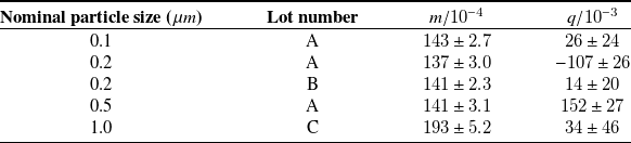
 m
 q

 μ
 z/wm
 z/wm
 z
 9
 z

 μ
 I¯
 x/w∈[−0.1,0.1]
 I¯
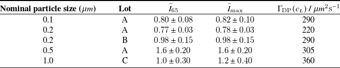
 I¯65
 z/w
 I¯max
 cL
 I¯65
 I¯max
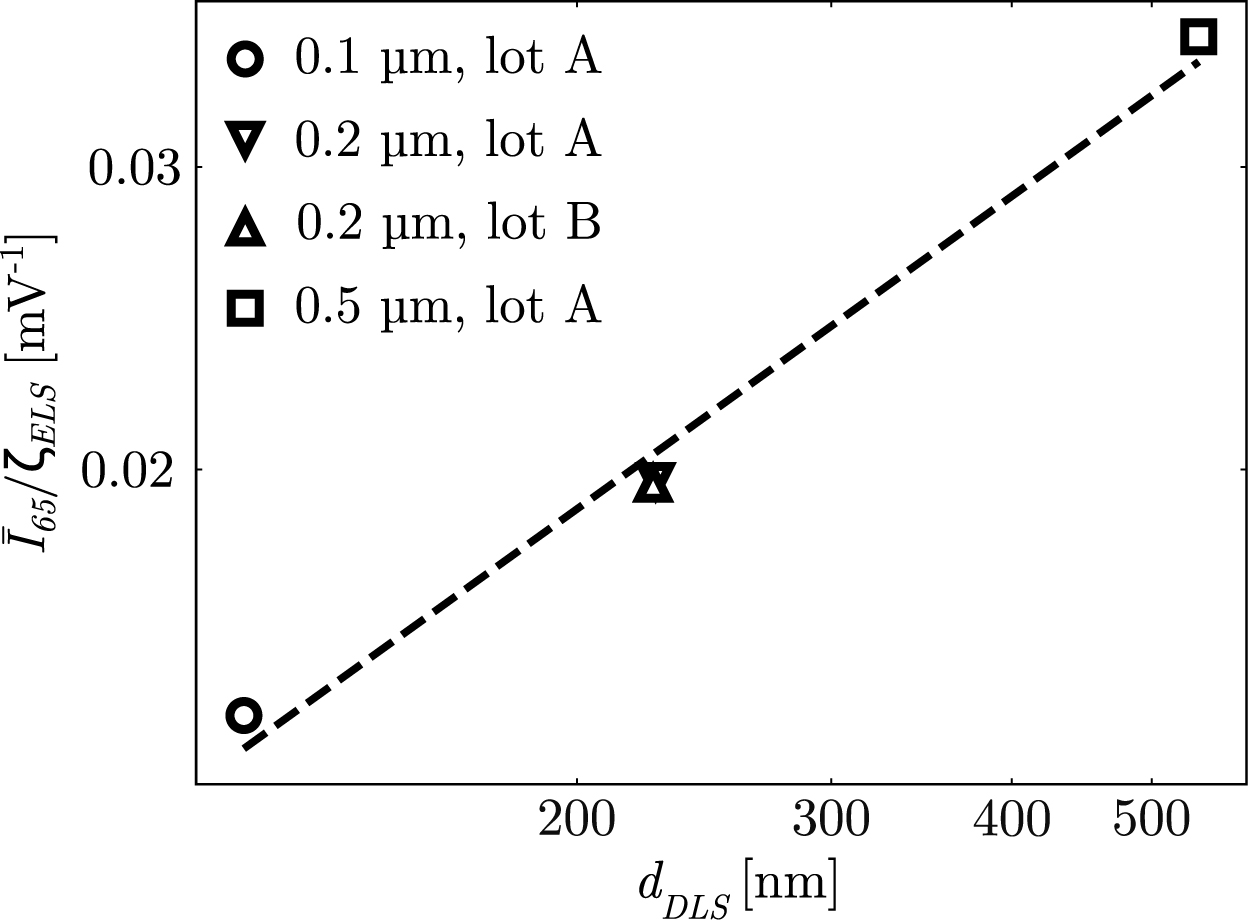
 z/w
 I¯65/ζELS
 dDLS
 cL

 dDLS
 ζELS
 dMF
 ζMF
 εd
 εζ
 dDLS
 dMF
 ζELS
 ζMF
 dDLS
 ζELS
 dMF
 ζMF


 Open access

