1 Introduction
A barrier or breakwater is a coastal structure which protects a coastline or marine structures or port or harbour from the effect of rough sea. A barrier, in the context of coastal engineering and marine structures, refers to a physical obstruction or structure that is primarily designed to impede or restrict the movement of water waves or other natural forces. Barriers are commonly used in coastal areas to protect land, infrastructure and human settlements from the destructive impacts of waves, storm surges and tidal currents. However, a breakwater is a specific type of barrier that is specifically designed to provide protection to a harbour, marina or other coastal structures by reducing the intensity of waves and creating a sheltered area behind it. Unlike barriers that are generally used to protect large stretches of coastlines, breakwaters are typically constructed in proximity to ports or harbours to create a safe haven for vessels and mitigate the effects of wave action.
Water wave scattering by floating breakwaters of varying shapes has been a central focus in the study of linearized water wave theory in the past few decades due to the following reasons:
-
(a) the construction of floating structures are cost effective compared with bottom founded structures;
-
(b) the floating structures allow better water circulation so that these have smaller impact on sediment transport and fish migration. This is the main advantage of floating structures over the bottom founded structures;
-
(c) in the recent past, the construction of floating structures are in demand as these structures are used as floating solar farms, floating hydrocarbon storage containers and many more. Hence, these floating structures serve as useful devices for human activities.
Researchers have employed various mathematical methods to examine how the waves interact with the structures. Thick breakwaters, with their larger and bulkier structure, are more effective at reducing wave energy compared with thin breakwaters. However, modern research has increasingly focused on breakwaters that combine both thin and thick parts, as they offer enhanced performance in various wave scattering scenarios. These hybrid structures combine the advantages of both types, providing effective wave attenuation while potentially optimizing material usage and reducing construction costs. Consequently, they have become a significant focus of research, especially in assessing their performance under varying wave conditions and environmental factors.
The rectangular or box-shaped breakwater is the most traditional design, valued for its simplicity and stability due to its substantial mass. It is particularly effective at reflecting wave energy, especially in the case of shorter-period waves, where its reflective properties are more noticeable. In this area of research, Mei and Black [Reference Mei and Black16] examined how surface gravity waves interact with both a rectangular bottom founded obstacle and a surface obstacle in finite-depth water.
Bai [Reference Bai2] used the finite element method to study wave scattering and diffraction forces acting on a fixed, elongated cylinder with a rectangular cross-section. McIver [Reference McIver15] examined the impact of wave interactions on a single floating bridge and a pair of adjacent floating bridges. He discovered that resonance occurred between the floating structures under specific combinations of wave and structural parameters. Abul-Azm and Gesraha [Reference Abul-Azm and Gesraha1] studied the interaction of oblique water waves with a long, rigid floating pontoon in finite ocean depth, considering both scattering and radiation effects. Mandal and Kanoria [Reference Kanoria, Dolai and Mandal11] employed Havelock expansion and integral equations to investigate oblique wave scattering caused by thick, horizontally fixed barriers of various configurations in finite-depth water. Based on their work, Das et al. [Reference Das, De and Mandal7] extended the work of Mandal and Kanoria [Reference Kanoria, Dolai and Mandal11], to analyse a floating and a submerged rectangular barrier, focusing on the reflection and transmission coefficients. The impact of a wave on a
 $\large \boldsymbol \sqcap $
-shaped breakwater was studied [Reference Gesraha8, Reference Kaligatla, Singh and Mandal10, Reference Singh, Kaligatla and Mandal20] by using the method of eigenfunction expansion. These problems were studied when the water region is of infinite depth or uniform finite depth. However, the nonuniformity at the bottom of the water region adds a significant effect to the wave scattering problems.
In 1981, Lee and Ayer [Reference Lee and Ayer14] applied the eigenfunction expansion method to study wave scattering by a symmetric trench. Miles [Reference Miles17] used conformal mapping to solve the trench problem for normally incident waves in 1982. Kirby and Dalrymple [Reference Kirby and Dalrymple12] extended this analysis to investigate obliquely incident surface waves diffracted by an asymmetric trench, employing linearized potential theory and resolving a set of integral equations through eigenfunction expansions. Subsequently, Kirby et al. [Reference Kirby, Dalrymple and Seo13] developed a theory for wave diffraction over a rectangular trench with currents flowing parallel to its boundaries. Chakraborty and Mandal [Reference Chakraborty and Mandal5, Reference Chakraborty and Mandal6] then investigated two-dimensional wave scattering by a rectangular submarine trench under both normal and oblique incidences, simplifying the problem to an integral equation that they solved using a multi-term Galerkin approximation with ultraspherical Gegenbauer polynomials. These studies enhance the understanding of wave behaviour in variable-depth environments, particularly around trenches. Later, Roy et al. [Reference Roy, Chakraborty and Mandal19] examined the scattering of water waves by an asymmetric rectangular trench using a method similar to that of Chakraborty and Mandal [Reference Chakraborty and Mandal5, Reference Chakraborty and Mandal6].
This study explores the problem of water wave scattering by a rectangular submarine trench in the presence of a
 $\large \boldsymbol \sqcap $
-shaped floating breakwater. This type of breakwater has a box with two thin legs at two sides. As mentioned earlier, this type of floating breakwater is used in floating oil storage and as a floating hydrocarbon storage container. Also, apart from cost effectiveness from a construction point of view, floating structures like this are advantageous ecologically as they allow sediment transport as well as fish migration. However, a
 $\large \boldsymbol \sqcap $
-shaped breakwater has several disadvantages related to its performance under specific wave conditions, complex structural behaviour and construction constraints. The geometric symmetry of the breakwater and the trench is used to divide the fluid domain into subregions, and this simplifies the related mixed boundary value problem considerably. By applying linear water wave theory, the velocity potentials in each sub-region are derived using Havelock’s expansions of the water wave potential. Suitable matching conditions at the interfaces of these subregions reduce the problem to two coupled Fredholm-type integral equations in unknown horizontal velocities across the interfaces. These coupled integral equations are then solved by using the multi-term Galerkin approximation technique [Reference Porter and Evans18] by employing orthogonal Chebyshev polynomials and ultraspherical Gegenbauer polynomials [Reference Gradshteyn and Ryzhik9] as basis functions. The basis functions as two types of special polynomials are chosen to accommodate the edge conditions at the submerged sharp tip of the breakwater and at the edge of the trench, respectively. At the corner points of the trench, the velocity has singularity of order
 $1/3$
, while at the tips of the legs of the
 $\large \boldsymbol \sqcap $
-shaped breakwater, the velocity has singularity of order
 $1/2$
. So, due to above-mentioned behaviour of the velocity function at the edges, this choice of ultraspherical Gegenbauer polynomials as basis functions to accommodate the singularity at the corner points of the trench and Chebyshev polynomials to accommodate the singularity at the tips of the legs of the
 $\large \boldsymbol \sqcap $
-shaped breakwater helps in convergence of the solution of the integral equation. This is the advantage in the choice of special polynomials as basis functions over any other simple polynomials.
We may mention that in the present method, the integral equations obtained are Fredholm type with regular kernel [Reference Banerjea and Mandal3]. However, this problem could have been tackled by other methods based on singular integral equation formulation. Nevertheless, the advantage of method based on integral equations with regular kernel are that regular integrals are more amenable to the numerical technique than a singular integral.
The reflection and transmission coefficients are explicitly derived and calculated approximately. The validity of these results is established through comparison with known findings in the literature. This study emphasizes the impact of various parameters, such as the submerged length of the side wall of the breakwater, width of the breakwater and depth of the trench, on the reflection and transmission coefficients as well as the wave forces on the breakwater. It is observed that the presence of a trench produces oscillation in the reflection and transmission coefficients. Also, when the width of the trench is equal to the width of the breakwater, reflection and transmission coefficients show smooth uniform oscillations. However, when the width of the trench and the width of the breakwater are unequal, nonuniform, nonsmooth oscillations in the reflection and transmission coefficients are observed and, in some cases, a resonance in the reflection coefficients is seen. It is also observed that the horizontal force exerted on the breakwater increases and the vertical force decreases as the length of the side wall of the
 $\large \boldsymbol \sqcap $
-shaped breakwater increases. Note that when the breakwater is present in a water region with a trench, the horizontal force is more than the vertical force. However, when the breakwater is present in uniformly deep water without a trench, the vertical force is more than the horizontal force.
2 Problem formulation
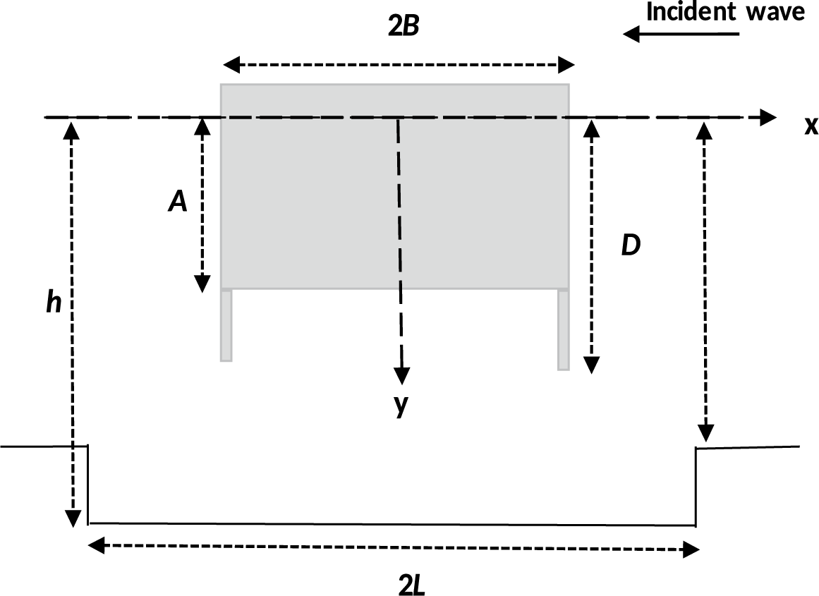
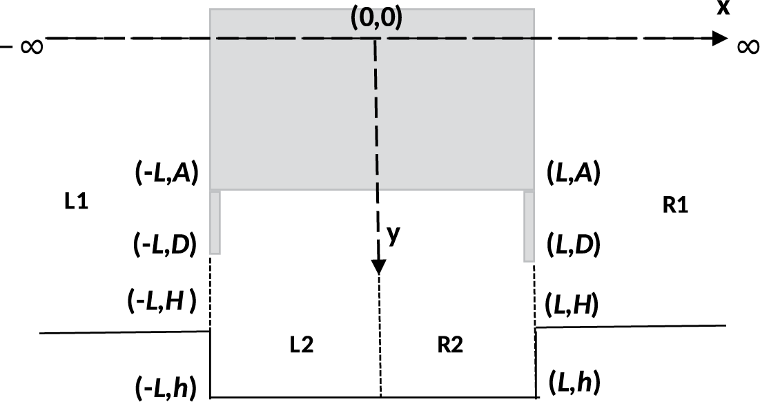
We consider a two-dimensional irrotational motion in water occupying the region
 $y \geq 0$
where the y-axis is taken vertically downwards into the fluid region and the x-axis along the mean free surface. A time harmonic wave train with angular frequency
 $\omega $
, from positive infinity, is incident normally on a
 $\large \boldsymbol \sqcap $
-shaped breakwater partially immersed in a water region with a submarine trench at the bottom. The impermeable breakwater comprises a box-type structure with two thin legs (the thickness of the legs is negligible). The box has width
 $2B$
and immersed length D, of which the immersed depth of the box part is A and the immersed legs have length
 $D-A$
. A rectangular submarine trench of width
 $2L $
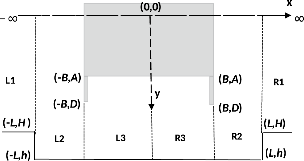
and depth h below the mean free surface is situated at the bottom of the water region (see Figure 1). Both the breakwater and trench have a geometrical symmetry with respect to the y-axis. The fluid region is divided into six regions given as follows:
Schematic diagram of the problem.

Region L1 –
 $\{(x,y)\mid \infty <x<-L,~0<y<H\}$
;
Region R1 –
 $\{(x,y)\mid L<x<\infty ,~0<y<H\}$
;
Region L2 –
 $\{(x,y)\mid L<x<-B,~0<y<h\}$
;
Region R2 –
 $\{(x,y)\mid B<x<L,~0<y<h\}$
;
Region L3 –
 $\{(x,y)\mid -B<x<0,~A<y <h\}$
;
Region R3 –
 $\{(x,y)\mid 0<x<B,~A<y <h\}$
.
Subregions of the fluid domain.

Assuming linear theory, the resulting motion is described by velocity potential
 $\Re \ \{\phi (x,y) e^{-i\omega t}\}$
, where
 $\phi (x,y)$
satisfies
 $$ \begin{align} \nabla^2{\phi}=0 \quad \text{in the water region}, \end{align} $$
the free surface boundary condition is
 $$ \begin{align} K \phi+ \phi_y=0 \quad \text{on } y=0,~|x|>B, \end{align} $$
conditions on the vertical sides of the trench are
 $$ \begin{align} \phi_x=0 \quad\text{at } x=\pm L,~H<y<h \quad \text{in Region R2, L2,} \end{align} $$
conditions on the vertical sides of the breakwater are
 $$ \begin{align} \phi_x=0 \quad \text{on } x=\pm B,~0<y<D \quad \text{in Region R2, L2,} \end{align} $$
 $$ \begin{align*} \phi_x=0 \quad \text{on } x=\pm B,~A<y<D \quad \text{in Region R3, L3,} \end{align*} $$
conditions on the horizontal side of the breakwater are
 $$ \begin{align} \phi_y=0 \quad \text{on~} y=A,~-B<x<B \quad \text{in Region R3, L3,} \end{align} $$
the bottom conditions are
 $$ \begin{align} \phi_y=0 \quad \text{at~} y=H,\quad |x|>L, \end{align} $$
 $$ \begin{align} \phi_y=0 \quad \text{at~} y=h,\quad |x|<L, \end{align} $$
the edge conditions are
 $$ \begin{align} r_{1}^{1/2} \nabla \phi \text{ is bounded as } r_{1} \rightarrow 0 \quad \text{where~} r_{1}=\sqrt{(x\pm B)^{2}+(y-D)^{2}}, \end{align} $$
 $$ \begin{align} r_{2}^{1/3} \nabla \phi \text{ is bounded as } r_{2} \rightarrow 0 \quad \text{where~} r_{2}=\sqrt{(x\pm L)^{2}+(y-H)^{2}}, \end{align} $$
and the far field conditions are given by
 $$ \begin{align} \phi(x,y)\longrightarrow \begin{cases} \dfrac{\cosh{P_0(H-y)e^{ -iP_0(x-L) }}}{\cosh{P_0 H}} ~+R ~\dfrac{\cosh{P_0(H-y)e^{ iP_0(x-L) }}}{\cosh{P_0 H}}&\quad \text{as } x \rightarrow \infty, \\[6pt] T~\dfrac{\cosh{P_0(H-y)e^{ -iP_0(x+L) }}}{\cosh{P_0 H}} & \quad \text{as } x\rightarrow -\infty, \end{cases} \end{align} $$
where R and T are the reflection and transmission coefficients (complex), respectively, to be determined, and
 $P_0$
is the unique real positive root of the dispersion relation
 $k \tanh {kH}=K, K={\omega ^2}/{g}$
, g is the acceleration due to gravity, and t is time.
3 Method of solution
The breakwater is symmetrical about
 $x=0$
. Therefore, we split the velocity potential into a symmetric part
 $\phi ^{a}(x,y)$
and an antisymmetric part
 $\phi ^{s}(x,y)$
, so that
 $$ \begin{align*} \phi(x,y)=\phi^{a}(x,y)+\phi^{s}(x,y), \end{align*} $$
where
 $$ \begin{align} \phi^{a}(-x,y)=\phi^{a}(x,y) \quad \text{and} \quad \phi^{s}(-x,y)=-\phi^{s}(x,y). \end{align} $$
Thus, the problem can be considered in the right half-plane
 $x\geq 0$
only in Regions R1, R2 and R3.
Note that
 $\phi ^{a}(x,y)$
and
 $\phi ^{s}(x,y)$
satisfy the relations (2.1)–(2.9). From (3.1), we get
 $$ \begin{align} \phi^{a}_x(0,y)=0,\quad 0<y<h, \end{align} $$
 $$ \begin{align} \phi^{s}(0,y)=0, \quad 0<y<h. \end{align} $$
Let the behaviour of
 $\phi ^{a,s}(x,y)$
be represented by
 $$ \begin{align*} \phi^{a,s}(x,y)\approx \frac{\cosh{P_0(H-y)}}{\cosh{P_0 H}}\{ e^{-iP_0(x-L)}+ \mathcal{ R}^{a,s} e^{iP_0(x-L)}\} \quad \text{as } x \rightarrow \infty. \end{align*} $$
Here,
 $\mathcal { R}^{a}, \mathcal { R}^{s}$
are unknown constants.
Using (2.10), we find that
 $\mathcal { R}^{a}$
and
 $\mathcal { R}^{s}$
are related to R and T by
 $$ \begin{align*} R=\dfrac{(\mathcal{ R}^{a}+\mathcal{ R}^{s})}{2} e^{-2iP_{0}L},\quad T= \dfrac{(\mathcal{ R}^{a}-\mathcal{ R}^{s})}{2} e^{-2iP_{0}L}. \end{align*} $$
3.1 Eigenfunction expansion for
 $\phi ^{a,s}(x,y)$
in various regions

The eigen expansion of
 $\phi ^{a,s}(x,y)$
satisfying (2.1)–(2.7), (3.2), (3.3) for
 $x\geq 0$
are given below.
Region R1
 $~(x>L,~0<y<H)$
 $$ \begin{align} \phi^{a,s}(x,y)&= \frac{\cosh{P_0(H-y)}}{\cosh{P_0 H}}\{e^{-iP_0(x-L)}+ \mathcal{R}^{a,s}e^{iP_0(x-L) }\}\nonumber \\ &\quad +\sum_{r=1}^{\infty}\mathcal{A}^{a,s}_{r}\cos P_{r}(H-y) e^{-P_r(x-L) }, \end{align} $$
where
 $k= P_{0}$
and
 $k= iP_{r}(r=1,2,\ldots )$
are the roots of the equation
 $$ \begin{align*} k\tanh kH-K=0 , \end{align*} $$
and
 $\mathcal {A}^{a,s}_{r},~ r=1,\ldots, \infty $
are unknowns to be determined.
Region R2
 $~(B<x<L,~0<y<h)$
 $$ \begin{align} \begin{pmatrix} \phi^{a}(x,y) \\ \phi^{s}(x,y) \end{pmatrix}=\begin{pmatrix} \mathcal{B}^{a}_{0}\cos p_{0}x \\ \mathcal{B}^{s}_{0}\sin p_{0}x \end{pmatrix} \frac{\cosh{p_0(h-y)}}{\cosh{p_0 h}}+\sum_{r=1}^{\infty}\begin{pmatrix} \mathcal{B}^{a}_{r}\cosh p_{r}x \\ \mathcal{B}^{s}_{r}\sinh p_{r}x \end{pmatrix}\cos p_{r}(h-y), \end{align} $$
where
 $k= p_{0}$
and
 $k= ip_{r}(r=1,2,\ldots )$
are the roots of the equation
 $$ \begin{align*} k\tanh kh-K=0, \end{align*} $$
and
 $\mathcal {B}^{a,s}_{r},~ r=0,1,\ldots, \infty $
are unknowns to be determined.
Region R3
 $~(0<x<B,~A<y<h)$
 $$ \begin{align} \begin{pmatrix} \phi^{a}(x,y) \\ \phi^{s}(x,y) \end{pmatrix}=\begin{pmatrix}\mathcal{ C}^{a}_{0} \\ \mathcal{ C}^{s}_{0}x \end{pmatrix} +\sum_{r=1}^{\infty}\begin{pmatrix} \mathcal{ C}^{a}_{r}\cosh \bigg(\dfrac{r\pi}{h-A}\bigg)x \\[.2cm] \mathcal{C}^{s}_{r}\sinh\bigg(\dfrac{r\pi}{h-A}\bigg)x \end{pmatrix}\cos\bigg(\dfrac{r\pi}{h-A}\bigg)(h-y), \end{align} $$
where
 $\mathcal {C}^{a,s}_{r},~ r=0,1,\ldots, \infty $
are unknowns to be determined.
3.2 Determination of unknowns in the eigenfunction expansion for
$\phi ^{a,s}(x,y)$

Let us now define
 $$ \begin{align} f^{a,s}(y)=\phi^{a,s}_{x}(L+0,y) \quad \text{for~} 0<y<H,~ \end{align} $$
 $$ \begin{align}\kern-6pt F^{a,s}(y)=\phi^{a,s}_{x}(L-0,y) \quad \text{for~} 0<y<h.~ \end{align} $$
Then,
 $$ \begin{align*} F^{a,s}(y)=\begin{cases} f^{a,s}(y) & \text{ for } 0<y<H, \\ 0 &\text{ for } H<y<h, \end{cases} \end{align*} $$
and
 $$ \begin{align}\kern-6pt G^{a,s}(y)=\phi^{a,s}_{x}(B+0,y) \quad \text{for } 0<y<h, \end{align} $$
 $$ \begin{align} g^{a,s}(y)=\phi^{a,s}_{x}(B-0,y) \quad \text{for } D<y<h. \end{align} $$
Then,
 $$ \begin{align*} G^{a,s}(y)= \begin{cases} 0 \quad & \text{ for }0<y<D, \\ g^{a,s}(y) & \text{ for }D<y<h. \end{cases} \end{align*} $$
The edge conditions given by (2.8) and (2.9) assert that
 $$ \begin{align*} F^{a,s}(y)&=O (|y-H|^{-{1}/{3}}) \quad \text{as~} y\rightarrow H, \\G^{a,s}(y)&=O (|y-D|^{-{1}/{2}}) \quad\text{as~} y\rightarrow D.\end{align*} $$
Using the expansion (3.4) in relation (3.7) and applying Havelock’s inversion formula, we obtain
 $$ \begin{align} 1-\mathcal{R}^{a,s}&=\frac{4 i \cosh{P_0H}}{\delta_{0}}\int_{0}^{H}f^{a,s}(y)\cosh{P_0(H-y)}~dy, \\\mathcal{A}_{r}^{a,s}&=-\frac{4}{\delta_{r}}\int_{0}^{H}f^{a,s}(y)\cos{P_r(H-y)}~dy ,\nonumber \end{align} $$
with
 $\delta _{0}=2P_0H+\sinh {2P_0H}$
and
 $\delta _{r}=2P_rH+\sin {2P_rH}$
for
 $r=1,2,3,\ldots .$
Using the expansion (3.5) in (3.8) and (3.9), and applying Fourier cosine transformation, we obtain
 $$ \begin{align*} \mathcal{B}_{0}^{a,s}&=\frac{4\cosh{p_0h}}{\gamma_{0}}\bigg(\dfrac{-1}{\sin{p_0L}},\dfrac{1}{\cos{p_0L}}\bigg)\int_{0}^{h}F^{a,s}(y)\cosh{p_0(h-y)}~dy \\ &=\frac{4\cosh{p_0h}}{\gamma_{0}}\bigg(\dfrac{-1}{\sin{p_0B}},\dfrac{1}{\cos{p_0B}}\bigg)\int_{0}^{h}G^{a,s}(y)\cosh{p_0(h-y)}~dy, \\ \mathcal{B}_{r}^{a,s}&=\frac{4}{\gamma_{r}}\bigg(\dfrac{1}{\sinh{p_rL}},\dfrac{1}{\cosh{p_rL}}\bigg)\int_{0}^{h}F^{a,s}(y)\cos{p_r(h-y)}~dy \\ &=\frac{4}{\gamma_{r}}\bigg(\dfrac{1}{\sinh{p_rB}},\dfrac{1}{\cosh{p_rB}}\bigg)\int_{0}^{h}G^{a,s}(y)\cos{p_r(h-y)}~dy, \end{align*} $$
with
 $\gamma _{0}=2p_0h+\sinh {2p_0h}$
and
 $\gamma _{r}=2p_rh+\sin {2p_rh}$
for
 $r=1,2,3,\ldots .$
Again, using (3.6) in (3.10) and applying Fourier cosine transformation, we get
 $$ \begin{align*} \mathcal{ C}_{0}^{s}&=\frac{1}{h-A }\int_{D}^{h}g^{s}(y)~dy, \\ \mathcal{ C}_{r}^{a,s}&=\frac{2}{r\pi}\bigg(\dfrac{1}{\sinh(\tfrac{r\pi}{h-A})B}, \dfrac{1}{\cosh(\tfrac{r\pi}{h-A})B}\bigg)\int_{D}^{h}g^{a,s}(y)\cos{\bigg(\dfrac{r\pi}{h-A}\bigg)(h-y)}~dy. \end{align*} $$
Thus, all the unknowns
 $\mathcal {R}^{a,s},~\mathcal { A}_{r}^{a,s},~ \mathcal { B}_{r}^{a,s}~ \text {and}~\mathcal { C}_{r}^{a,s}$
are expressed in terms of unknown functions
 $F^{a,s}(y)$
and
 $G^{a,s}(y)$
. Next, we shall derive integral equations for the functions
 $F^{a,s}(y)$
and
 $G^{a,s}(y)$
.
3.3 Integral equations for
$F^{a,s}(y)$
and
$G^{a,s}(y)$


We consider the continuity of the functions
 $\phi ^{a,s}(x,y)$
across the gaps in the boundaries of the different regions.
At the interface of Regions
 $R1$
and
 $R2$
, that is, at
 $x=L$
,
 $$ \begin{align*} \phi^{a,s}(L+0,y)=\phi^{a,s}(L-0,y), \quad 0<y<H. \end{align*} $$
In the gap below the barrier at the interface of Regions
 $R2$
and
 $R3$
, that is, at
 $x=B$
,
 $$ \begin{align*} \phi^{a,s}(B+0,y)=\phi^{a,s}(B-0,y),\quad D<y<h. \end{align*} $$
These matching conditions provide the following system of integral equations for
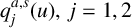 $q_{j}^{a,s}(u),~j=1,2$
:
 $$ \begin{align} \int_{0}^{H}q_{1}^{a,s}(u)M_{1}^{a,s}(y,u)\,du+\int_{D}^{h}q_{2}^{a,s}(u)N_{1}^{a,s}(y,u)\,du=X_{1}^{a,s},\quad 0<y<H,~ \end{align} $$
 $$ \begin{align} \int_{0}^{H}q_{1}^{a,s}(u)M_{2}^{a,s}(y,u)\,du+\int_{D}^{h}q_{2}^{a,s}(u)N_{2}^{a,s}(y,u)\,du=X_{2}^{a,s},\quad D<y<h,~ \end{align} $$
where
 $$ \begin{align} q_{1}^{a,s}(u)&=\dfrac{f^{a,s}(u)}{1+\mathcal{ R}^{a,s}}, \nonumber \\ q_{2}^{a,s}(u)&=\dfrac{g^{a,s}(u)}{1+\mathcal{ R}^{a,s}}, \\ X_{1}^{a,s}&=\frac{\cosh{P_0(H-y)}}{\cosh{P_0 H}}, \nonumber \\ X_{2}^{a,s}&=0, \nonumber \end{align} $$
and the kernels
 $$ \begin{align*} M_{1}^{a,s}(y,u)&=\sum_{r=1}^{\infty}\dfrac{4}{\delta_{r}}\cos P_{r}(H-u)\cos P_{r}(H-y), \\M_{2}^{a}(y,u)&=\dfrac{4\cos p_{0}B}{\gamma_{0}\sin p_{0}L}\cosh p_{0}(h-u)\bigg\{\cosh p_{0}(h-y)-\dfrac{\sinh p_{0}(h-D)}{p_{0}(h-D)}\bigg\} \nonumber \\&\quad -\sum_{r=1}^{\infty}\dfrac{4\cosh p_{r}B}{\gamma_{r}\sinh p_{r}L}\cos p_{r}(h-u)\bigg\{\cos p_{r}(h-y)-\dfrac{\sin p_{r}(h-D)}{p_{r}(h-D)}\bigg\}, \\M_{2}^{s}(y,u)&=\dfrac{4\sin p_{0}B}{\gamma_{0}\cos p_{0}L}\cosh p_{0}(h-u)\cosh p_{0}(h-y) \nonumber \\&\quad +\sum_{r=1}^{\infty}\dfrac{4\sinh p_{r}B}{\gamma_{r}\cosh p_{r}L}\cos p_{r}(h-u)\cos p_{r}(h-y), \\N_{1}^{a}(y,u)&=-\dfrac{4\cos p_{0}L}{\gamma_{0}\sin p_{0}B}\cosh p_{0}(h-u)\cosh p_{0}(h-y) \nonumber \\&\quad + \sum_{r=1}^{\infty}\dfrac{4\cosh p_{r}L}{\gamma_{r}\sinh p_{r}B}\cos p_{r}(h-u)\cos p_{r}(h-y), \\N_{1}^{s}(y,u)&=\dfrac{4\sin p_{0}L}{\gamma_{0}\cos p_{0}B}\cosh p_{0}(h-u)\cosh p_{0}(h-y) \nonumber \\&\quad +\sum_{r=1}^{\infty}\dfrac{4\sinh p_{r}L}{\gamma_{r}\cosh p_{r}B}\cos p_{r}(h-u)\cos p_{r}(h-y),\\N_{2}^{a}(y,u)&=\sum_{r=1}^{\infty}\dfrac{2}{r\pi}\coth \bigg(\dfrac{r\pi}{h-A}\bigg)B\cos\bigg(\dfrac{r\pi}{h-A}\bigg)(h-u)\bigg\{\cos\bigg(\dfrac{r\pi}{h-A}\bigg)(h-y) \nonumber \\&\quad -\frac{1}{r\pi}\bigg(\frac{h-A}{h-D}\bigg)\sin\bigg(\dfrac{r\pi}{h-A}\bigg)(h-D)\bigg\}, \\N_{2}^{s}(y,u)&=\dfrac{-B}{h-A}-\sum_{r=1}^{\infty}\dfrac{2}{r\pi}\tanh \bigg(\dfrac{r\pi}{h-A}\bigg)B\cos\bigg(\dfrac{r\pi}{h-A}\bigg)(h-u)\cos\bigg(\dfrac{r\pi}{h-A}\bigg)(h-y). \end{align*} $$
The substitution of
 $q_{1}^{a,s}(y)$
from (3.13) into (3.11) gives rise to
 $$ \begin{align} \frac{4\cosh{P_0H}}{\delta_{0}}\int_{0}^{H}q_{1}^{a,s}(y)\cosh P_{0}(H-y)~dy=C^{a,s}, \end{align} $$
where
 $$ \begin{align} C^{a,s}=-i\dfrac{1-\mathcal{R}^{a,s}}{1+\mathcal{R}^{a,s}}. \end{align} $$
Using (3.15), the reflection and transmission coefficient are obtained as
 $$ \begin{align} |R|=\dfrac{|1+C^{a}C^{s}|}{\Delta},\quad |T|=\dfrac{|C^{a}-C^{s}|}{\Delta}, \end{align} $$
where
 $\Delta =\{1+(C^{a})^{2}+(C^{s})^{2}+(C^{a}C^{s})^{2}\}^{{1}/{2}}.$
Thus, solving the system of integral equations (3.12a), (3.12b), the functions
 $q_j,~j=1,2$
are determined which are then used in (3.14)–(3.16) to evaluate
 $|R|$
and
 $|T|$
.
Also, the horizontal force and vertical force on the
 $\large \boldsymbol \sqcap $
-shaped breakwater can be determined by using Bernoulli’s equation [Reference Bai2, Reference Bhattacharjee and Soares4, Reference Kaligatla, Singh and Mandal10] and is given by
 $$ \begin{align*} W_{h1}&=2 i\rho \omega \, \bigg(\!\int_{0}^{D}{\phi^{s}(B+0,y)}\,dy-\int_{A}^{D}{\phi^{s}(B-0,y)}\, dy\bigg),\\ W_{v1}&=2 i\rho \omega\int_{0}^{B}{\phi^{a}(x,A)}\,dx, \end{align*} $$
where
 $W_{h1}$
is the horizontal force and
 $W_{v1}$
is the vertical force.
The horizontal force and vertical force per unit width can be expressed in the nondimensional form as
 $$ \begin{align*} W_{h}=\dfrac{|W_{h1}|}{\rho g \xi B}, \quad W_{v}=\dfrac{|W_{v1}|}{\rho g \xi B}. \end{align*} $$
Here,
 $\xi $
is the incident wave amplitude and
 $\rho $
is the density of the water.
3.4 Solution of integral equations by the Galerkin method
Now, we solve the integral equations (3.12a), (3.12b) using the multi-term Galerkin approximation method involving orthogonal polynomials multiplied by appropriate weight functions as basis functions. Here, it is important to note that the choice of basis functions depends on the types of singularities at the corner of the trench and at the submerged sharp edge of the breakwater as given by the edge conditions (2.8), (2.9).
Noting the edge condition (2.9), we express the unknown function
 $q_{1}^{a,s}(y)$
in terms of Gegenbauer polynomials and noting the edge condition (2.8), we express the unknown function
 $q_{2}^{a,s}(y)$
in terms of Chebychev’s polynomial as
 $$ \begin{align} q_{1}^{a,s}(y)&=\sum_{n=0}^{N}a_{n}^{a,s}U_{n}^{a,s}(y),\quad 0<y<H, \end{align} $$
 $$ \begin{align} q_{2}^{a,s}(y)&=\sum_{n=0}^{N}b_{n}^{a,s}V_{n}^{a,s}(y),\quad D<y<h. \end{align} $$
Here,
 $$ \begin{align*} U_{n}^{a,s}(y)=U_{n}(y)=-\frac{d}{dy}\bigg[e^{-Ky}\int_{y}^{H}e^{Kz}\tilde{U_{n}}(z)\,dz\bigg],\quad 0<y<H, \end{align*} $$
with
 $$ \begin{align*} \tilde{U_{n}}(z)=\dfrac{2^{{7}/{6}}\Gamma({1}/{6})(2n)!}{\pi \Gamma(2n+{1}/{3})H^{{1}/{3}}(H^{2}-z^{2})^{{1}/{3}}}C_{2n}^{{1}/{6}}\bigg(\dfrac{z}{H}\bigg),\quad n=0,1,2,\ldots, \end{align*} $$
where
 $C_{2n}^{{1}/{6}}({z}/{H})$
are Gegenbauer polynomials of order
 $({1}/{6})$
, and
 $$ \begin{align*} V_{n}^{a,s}(y)=V_{n}(y)=\dfrac{2(-1)^{n}}{\pi \{(h-D)^{2}-(h-y)^{2}\}^{{1}/{2}}}T_{2n}\bigg(\dfrac{h-y}{h-D}\bigg),\quad D<y<H, \end{align*} $$
where
 $T_{2n}(y)$
are Chebychev’s polynomial of first kind of order
 $2n$
.
We substitute the expansion (3.17) and (3.18) in (3.12a), then multiplying by
 $U_{m}^{a,s}(y)$
and integrating y from
 $0$
to H, we get
 $$ \begin{align} &\sum_{n=0}^{N}a_{n}^{a,s}\int_{0}^{H}\int_{0}^{H}M_{1}^{a,s}(y,u)U_{n}^{a,s}(u)U_{m}^{a,s}(y)\,du\,dy \nonumber \\ &\quad +\sum_{n=0}^{N}b_{n}^{a,s}\int_{0}^{H}\int_{D}^{h}N_{1}^{a,s}(y,u)V_{n}^{a,s}(u)U_{m}^{a,s}(y)\,du\,dy =\int_{0}^{H}\frac{\cosh{P_0(H-y)}}{\cosh{P_0 H}}U_{m}^{a,s}(y)\,dy,\nonumber \\ &\sum_{n=0}^{N}a_{n}^{a,s}K_{1mn}^{a,s}+\sum_{n=0}^{N}b_{n}^{a,s}J_{1mn}^{a,s}=d_{1m,}^{a,s},\quad m=0,1,\ldots ,N. \end{align} $$
Again substituting the expansion (3.17) and (3.18) in (3.12b), multiplying by
 $V_{m}^{a,s}(y)$
and integrating y from D to h, we get
 $$ \begin{align} &\sum_{n=0}^{N}a_{n}^{a,s}\int_{D}^{h}\int_{0}^{H}M_{2}^{a,s}(y,u)U_{n}^{a,s}(u)V_{m}^{a,s}(y)\,du\,dy\nonumber \\ &\quad +\sum_{n=0}^{N}b_{n}^{a,s}\int_{D}^{h}\int_{D}^{h}N_{2}^{a,s}(y,u)V_{n}^{a,s}(u)V_{m}^{a,s}(y)\,du\,dy =0,\nonumber \\ &\sum_{n=0}^{N}a_{n}^{a,s}K_{2mn}^{a,s}+\sum_{n=0}^{N}b_{n}^{a,s}J_{2mn}^{a,s}=d_{2m,}^{a,s},\quad m=0,1,\ldots ,N, \end{align} $$
where
 $$ \begin{align*} K_{1mn}^{a,s}&=\int_{0}^{H}\int_{0}^{H}M_{1}^{a,s}(y,u)U_{n}^{a,s}(u)U_{m}^{a,s}(y)\,du\,dy \\ &=\sum_{r=1}^{\infty}(-1)^{m+n}\dfrac{16}{\delta_{r}}\dfrac{\cos^{2}P_{r}H}{(P_{r}H)^{{1}/{3}}}J_{2m+{1}/{6}}(P_{r}H)J_{2n+{1}/{6}}(P_{r}H), \\ J_{1mn}^{a}&=\int_{D}^{h}\int_{0}^{H}N_{1}^{a}(y,u)V_{n}^{a}(u)U_{m}^{a}(y)\,du\,dy \\ &=(-1)^{n+1}\dfrac{8}{\gamma_{0}}\dfrac{\cos p_{0}L}{\sin p_{0}B}\dfrac{\cosh p_{0}h}{(p_{0}H)^{{1}/{6}}}I_{2n}(p_{0}(h-D))I_{2m+{1}/{6}}(p_{0}H) \\ &\quad +\sum_{r=1}^{\infty}(-1)^{m}\dfrac{8}{\gamma_{r}}\dfrac{\cosh p_{r}L}{\sinh p_{r}B}\dfrac{\cos p_{r}h}{(p_{r}H)^{{1}/{6}}}J_{2n}(p_{r}(h-D))J_{2m+{1}/{6}}(p_{r}H), \end{align*} $$
 $$ \begin{align*} J_{1mn}^{s}&=\int_{D}^{h}\int_{0}^{H}N_{1}^{s}(y,u)V_{n}^{s}(u)U_{m}^{s}(y)\,du\,dy \nonumber\\&=(-1)^{n}\dfrac{8}{\gamma_{0}}\dfrac{\sin p_{0}L}{\cos p_{0}B}\dfrac{\cosh p_{0}h}{(p_{0}H)^{{1}/{6}}}I_{2n}(p_{0}(h-D))I_{2m+{1}/{6}}(p_{0}H)\nonumber\\&\quad +\sum_{r=1}^{\infty}(-1)^{m}\dfrac{8}{\gamma_{r}}\dfrac{\sinh p_{r}L}{\cosh p_{r}b}\dfrac{\cos p_{r}h}{(p_{r}H)^{{1}/{6}}}J_{2n}(p_{r}(h-D))J_{2m+{1}/{6}}(p_{r}H), \\K_{2mn}^{a}&=\int_{D}^{h}\int_{0}^{H}M_{2}^{a}(y,u)U_{n}^{a}(u)V_{m}^{a}(y)\,du\,dy \nonumber\\[3pt]&=(-1)^{m}\dfrac{8}{\gamma_{0}}\dfrac{\cos p_{0}B}{\sin p_{0}L}\dfrac{\cosh p_{0}h}{(p_{0}H)^{{1}/{6}}}I_{2n+{1}/{6}}(p_{0}H)I_{2m}(p_{0}(h-D))\nonumber\\[3pt]&\quad -\sum_{r=1}^{\infty}(-1)^{n}\dfrac{8}{\gamma_{r}}\dfrac{\cosh p_{r}B}{\sinh p_{r}L}\dfrac{\cos p_{r}h}{(p_{r}H)^{{1}/{6}}}J_{2n+{1}/{6}}(p_{r}H)J_{2m}(p_{r}(h-D)) , \\[3pt]K_{2mn}^{s}&=\int_{D}^{h}\int_{0}^{H}M_{2}^{s}(y,u)U_{n}^{s}(u)V_{m}^{s}(y) \,du\,dy \nonumber\\[3pt]&=(-1)^{m}\dfrac{8}{\gamma_{0}}\dfrac{\sin p_{0}B}{\cos p_{0}L}\dfrac{\cosh p_{0}h}{(p_{0}H)^{{1}/{6}}}I_{2n+{1}/{6}}(p_{0}H)I_{2m}(p_{0}(h-D))\nonumber\\[3pt]&\quad -\sum_{r=1}^{\infty}(-1)^{n+1}\dfrac{8}{\gamma_{r}}\dfrac{\sinh p_{r}B}{\cosh p_{r}L}\dfrac{\cos p_{r}h}{(p_{r}H)^{{1}/{6}}}J_{2n+{1}/{6}}(p_{r}H)J_{2m}(p_{r}(h-D)), \\[3pt]J_{2mn}^{a}&=\int_{D}^{h}\int_{D}^{h}N_{2}^{a}(y,u)V_{n}^{a}(u)V_{m}^{a}(y)\,du\,dy \nonumber\\[3pt]&=\sum_{r=1}^{\infty}\dfrac{2}{r\pi}\coth\bigg(\dfrac{r\pi}{h-A}\bigg)BJ_{2n}\bigg(\dfrac{r\pi}{h-A}(h-D)\bigg)J_{2m}\bigg(\dfrac{r\pi}{h-A}(h-D)\bigg), \end{align*} $$
 $$ \begin{align} J_{2mn}^{s}&=\int_{D}^{h}\int_{D}^{h}N_{2}^{s}(y,u)V_{n}^{s}(u)V_{m}^{s}(y)\,du\,dy \nonumber\\[3pt]&=\sum_{r=1}^{\infty}\dfrac{-2}{r\pi}\tanh\bigg(\dfrac{r\pi}{h-A}\bigg)BJ_{2n}\bigg(\dfrac{r\pi}{h-A}(h-D)\bigg)J_{2m}\bigg(\dfrac{r\pi}{h-A}(h-D)\bigg), \end{align} $$
 $$ \begin{align}\kern11pt d_{1m}^{a,s}&=\int_{0}^{H}\frac{\cosh{P_0(H-y)}}{\cosh{P_0 H}}U_{m}^{a,s}(y)\,dy=\dfrac{2}{(P_{0}H)^{{1}/{6}}}I_{2m+{1}/{6}}(P_{0}H)\quad \text{and} \end{align} $$
 $$ \begin{align}\kern6pt d_{2m}^{a,s}&=0. \qquad\qquad\qquad\qquad\qquad\qquad\qquad\qquad\quad\qquad\qquad\qquad\end{align} $$
Here,
 $J_\nu (x)$
is a Bessel function of first kind of order
 $\nu $
and
 $I_\nu (x)$
is a modified Bessel function of first kind of order
 $\nu $
.
The constants
 $a_{n}^{a,s},b_{n}^{a,s}(n=0,1,\ldots ,N)$
are now obtained by solving the linear systems (3.19), (3.20). Knowing
 $a_{n}^{a,s},b_{n}^{a,s}(n=0,1,\ldots ,N)$
, the functions
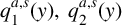 $q_{1}^{a,s}(y),~ q_{2}^{a,s}(y)$
can be evaluated from (3.17) and (3.18). Hence, using the function
 $q_{1}^{a,s}(y)$
, the relation (3.14) produces
 $$ \begin{align*} C^{a,s}=\dfrac{8\cosh^{2}P_{0}H}{\delta_{0}(P_{0}H)^{{1}/{6}}}\sum_{n=0}^{N}a_{n}^{a,s}I_{2n+{1}/{6}}(P_{0}H). \end{align*} $$
Once
 $C^{a,s}$
are determined,
 $|R|,|T| $
can be evaluated from (3.16).
3.5 Expression for fluid velocities in various regions
-
(I) Region R1
$~(x>L,~0<y<H)$
$$ \begin{align*} \phi_{x}(x,y)&= -4P_0 \frac{\cosh{P_0(H-y)}}{\cosh{P_0 H}}\bigg[\sin{P_0(x-L)}\cos \omega t-\dfrac{4 i}{\delta_{0}}\dfrac{(\cosh P_{0}H)^2}{(P_{0}H)^{{1}/{6}}} \nonumber\\ &\quad \times \sin(P_0(x-L)-\omega t) \sum_{n=0}^{N}\bigg\{\dfrac{a_{n}^{a}}{(1+iC^{a})} +\dfrac{a_{n}^{s}}{(1+iC^{s})}\bigg\}I_{2n+{1}/{6}}(P_{0}H)\bigg] \nonumber\\ &\quad +\sum_{r=1}^{\infty}\dfrac{16P_r}{\delta_{r}}\dfrac{\cos P_{r}H}{(P_{r}H)^{{1}/{6}}}\cos P_{r}(H-y)e^{-P_r(x-L)}\nonumber \\ &\quad\times\cos \omega t\sum_{n=0}^{N}\bigg\{\dfrac{a_{n}^{a}}{(1+iC^{a})} +\dfrac{a_{n}^{s}}{(1+iC^{s})}\bigg\}(-1)^nJ_{2n+{1}/{6}}(P_{r}H), \nonumber \end{align*} $$
$$ \begin{align*} \phi_{y}(x,y)&= 4P_0 \frac{\sinh{P_0(H-y)}}{\cosh{P_0 H}}\bigg[\cos{P_0(x-L)}\cos \omega t-\dfrac{4 i}{\delta_{0}}\dfrac{(\cosh P_{0}H)^2}{(P_{0}H)^{{1}/{6}}} \nonumber\\ &\quad \times \cos(P_0(x-L)-\omega t) \sum_{n=0}^{N}\bigg\{\dfrac{a_{n}^{a}}{(1+iC^{a})} +\dfrac{a_{n}^{s}}{(1+iC^{s})}\bigg\}I_{2n+{1}/{6}}(P_{0}H)\bigg] \nonumber\\ &\quad +\sum_{r=1}^{\infty}\dfrac{16P_r}{\delta_{r}}\dfrac{\cos P_{r}H}{(P_{r}H)^{{1}/{6}}}\sin P_{r}(H-y)e^{-P_r(x-L)}\nonumber \\ &\quad\times \cos \omega t\sum_{n=0}^{N}\bigg\{\dfrac{a_{n}^{a}}{(1+iC^{a})} +\dfrac{a_{n}^{s}}{(1+iC^{s})}\bigg\}(-1)^nJ_{2n+{1}/{6}}(P_{r}H). \nonumber \end{align*} $$
-
(II) Region R2
$~(B<x<L,~0<y<h)$
$$ \begin{align*} \phi_{x}(x,y) & = \dfrac{16p_0}{\gamma_{0}}\dfrac{\cosh p_{0}h}{(p_{0}H)^{{1}/{6}}}\cosh p_{0}(h-y)\cos \omega t \sum_{n=0}^{N}\bigg\{\dfrac{a_{n}^{a}}{(1+iC^{a})}\dfrac{\sin{p_{0}x}}{\sin{p_{0}L}} \nonumber\\ &\quad +\dfrac{a_{n}^{s}} {(1+iC^{s})}\dfrac{\cos{p_{0}x}}{\cos{p_{0}L}}\bigg\} I_{2n+{1}/{6}}(p_{0}H)\nonumber\\ &\quad +\sum_{r=1}^{\infty}\dfrac{16p_r}{\gamma_{r}}\dfrac{\cos p_{r}h}{(p_{r}H)^{{1}/{6}}}\cos p_{r}(h-y)\cos \omega t \nonumber\\ &\quad \times \sum_{n=0}^{N}(-1)^n \bigg\{\dfrac{a_{n}^{a}}{(1+iC^{a})}\dfrac{\sinh{p_{r}x}}{\sinh{p_{r}L}}+\dfrac{a_{n}^{s}}{(1+iC^{s})}\dfrac{\cosh{p_{r}x}}{\cosh{p_{r}L}}\bigg\}J_{2n+{1}/{6}}(P_{r}H), \nonumber \end{align*} $$
$$ \begin{align*} \phi_{y}(x,y)&= \dfrac{16p_0}{\gamma_{0}}\dfrac{\cosh p_{0}h}{(p_{0}H)^{{1}/{6}}}\sinh p_{0}(h-y)\cos \omega t\sum_{n=0}^{N}\bigg\{-\dfrac{a_{n}^{a}}{(1+iC^{a})}\dfrac{\cos{p_{0}x}}{\sin{p_{0}L}} \nonumber\\ &\quad +\dfrac{a_{n}^{s}}{(1+iC^{s})}\dfrac{\sin{p_{0}x}}{\cos{p_{0}L}}\bigg\} I_{2n+{1}/{6}}(p_{0}H) \nonumber\\ &\quad -\sum_{r=1}^{\infty}\dfrac{16p_r}{\gamma_{r}}\dfrac{\cos p_{r}h}{(p_{r}H)^{{1}/{6}}}\sin p_{r}(h-y)\cos \omega t \nonumber\\ &\quad \times \sum_{n=0}^{N}(-1)^n \bigg\{\dfrac{a_{n}^{a}}{(1+iC^{a})}\dfrac{\cosh{p_{r}x}}{\sinh{p_{r}L}}+\dfrac{a_{n}^{s}}{(1+iC^{s})}\dfrac{\sinh{p_{r}x}}{\cosh{p_{r}L}}\bigg\}J_{2n+{1}/{6}}(P_{r}H). \nonumber \end{align*} $$
-
(III) Region R3
$~(0<x<B,~A<y<h)$
$$ \begin{align*} \phi_{x}(x,y)&=\dfrac{4}{h-A}\sum_{r=1}^{\infty}\cos{\bigg(\dfrac{r\pi}{h-A}\bigg)(h-y)}\cos \omega t \nonumber \\ &\quad \times\sum_{n=0}^{N}\bigg\{\dfrac{b_{n}^{a}}{(1+iC^{a})}\dfrac{\sinh{(\tfrac{r\pi}{h-A})x}}{\sinh{(\tfrac{r\pi}{h-A})B}} +\dfrac{b_{n}^{s}}{(1+iC^{s})}\dfrac{\cosh{(\tfrac{r\pi}{h-A})x}}{\cosh{(\tfrac{r\pi}{h-A})B}}\bigg\} \nonumber \\ &\quad\times J_{2n}\bigg(\dfrac{r\pi}{h-A}(h-d)\bigg), \nonumber \end{align*} $$
$$ \begin{align*} \phi_{y}(x,y)&=\dfrac{-4}{h-A}\sum_{r=1}^{\infty}\sin{(\dfrac{r\pi}{h-A})(h-y)}\cos \omega t\nonumber \\ &\quad\times\sum_{n=0}^{N}\bigg\{\dfrac{b_{n}^{a}}{(1+iC^{a})}\dfrac{\cosh{(\tfrac{r\pi}{h-A})x}}{\sinh{(\tfrac{r\pi}{h-A})B}} +\dfrac{b_{n}^{s}}{(1+iC^{s})}\dfrac{\sinh{(\tfrac{r\pi}{h-A})x}}{\cosh{(\tfrac{r\pi}{h-A})B}}\bigg\} \nonumber \\ &\quad\times J_{2n}\bigg(\dfrac{r\pi}{h-A}(h-d)\bigg). \nonumber \end{align*} $$





3.6 Energy balance relation
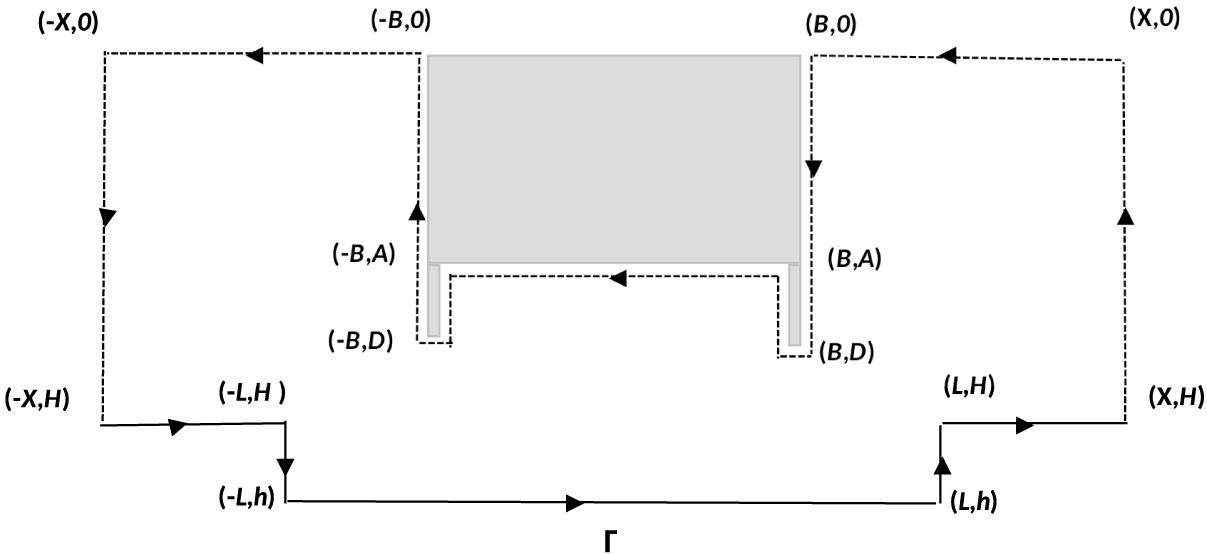
The energy balance is obtained by applying Green’s integral theorem to the functions
 $\phi (x,y)$
and
 $\bar {\phi (x,y)}$
in the region bounded by contour
 $\Gamma $
shown in Figure 3. This gives
 $$ \begin{align*} \int_\Gamma \bigg(\phi~ \frac{\partial \bar{\phi}}{\partial n}- \bar{\phi}~ \frac{\partial \phi}{\partial n}\bigg)\,d\Gamma=0. \end{align*} $$
Computing the integrals on different boundaries using the boundary conditions (2.2)–(2.10), we obtain the energy identity as
 $$ \begin{align} |R|^2+ |T|^2= 1. \end{align} $$
Schematic diagram.

4 Numerical results
In this section, the numerical results for reflection coefficient and transmission coefficient are computed numerically, and depicted graphically against the dimensionless wave number
 $KH$
in the figures for nondimensional values of
 $A/H,~ B/H,~ D/H, h/H,~ L/H$
.
4.1 Convergence of the method
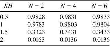
For numerical computation, the value of N in (3.19), (3.20) is chosen as
 $N=6$
. Table 1 depicts the convergence of
 $|R|$
. Here, some representative values of
 $|R|$
are presented for various
 $KH$
, taking
 $N=2,~4,~6$
and
 $A/H = 0.25,~ B/H=0.7,~ D/H= 0.45,~ h/H=1.1,~ L/H=0.8$
. It is observed from Table 1 that the values of
 $|R|$
coincide up to 3 to 4 decimal places for
 $N=4,~ 6$
.
Reflection coefficient for
 $B/H =0.7,~ A/H = 0.25,~ D/H=0.45,~ L/H=0.8,~ h/H=1.1$
.

4.2 Energy identity
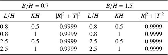
In Table 2, the energy identity (3.24) is verified and presented for various values of
 $KH$
and for
 $A/H = 0.25,~ D/H=0.45,~ h/H=1.2,~ L/H= 0.8, 2.5,~ B/H= 0.7,~ 1.5.$
Table 2 establishes the validity of energy balance relation.
Energy identity table for
 $A/H = 0.25,~ D/H=0.45,~ h/H=1.2$
.

4.3 Comparison of the results obtained with known results
In this section, the results obtained in the present study are authenticated by comparing the values of
 $|R|$
with the known results in the literature.
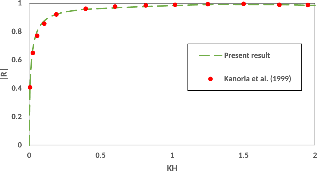
In Figure 4,
 $|R|$
obtained in the present study is compared with the results of Kanoria et al. [Reference Kanoria, Dolai and Mandal11] considering
 ${h/H = 1,~L/H = 0.0000001,~ A/H = 0.2,~B/H = 1,~D/H=0.2.}$
With these values of parameters
 $h/H,~L/H,~ A/H ,~B/H,~D/H$
, the
 $\sqcap $
-shaped breakwater reduces to a rectangular box present in water with a uniform bottom. The reflection coefficient
 $|R|$
thus obtained agrees very well with the results of Kanoria et al. [Reference Kanoria, Dolai and Mandal11].
Comparison between the present method and [Reference Kanoria, Dolai and Mandal11, Figure 2(a)] for
 $B/H = 1,A/H = 0.2, D/H=0.2$
.

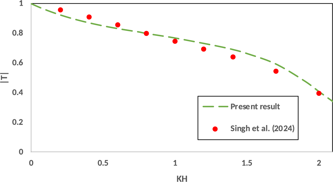
In Figure 5,
 $|T|$
obtained from the present analysis is compared with the results of Singh et al. [Reference Singh, Kaligatla and Mandal20] for
 $h/H = 1,~L/H = 0.005 ,~A/H = 0.25,~B/H = 0.5,~D/H=0.45$
. A good matching of the result is observed in the figure.
Comparison between the present method and [Reference Singh, Kaligatla and Mandal20, Figure 6] for
 $B/H = 0.5,~A/H = 0.25, D/H=0.45$
.

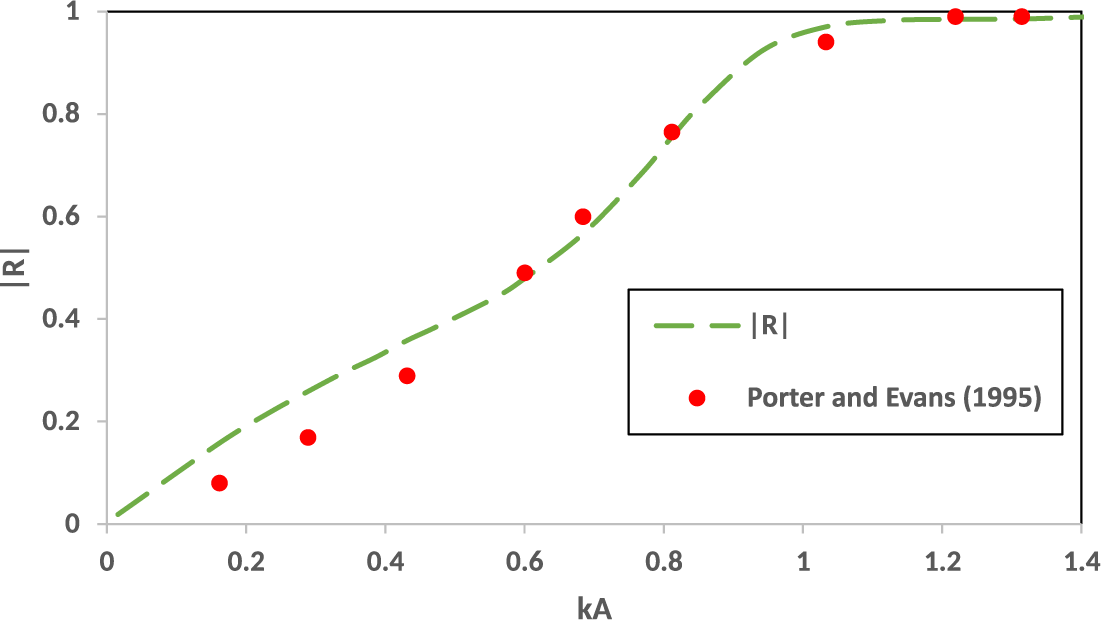
Porter and Evans [Reference Porter and Evans18] considered the problem of water wave diffraction by a thin rigid barrier partially immersed in water of uniform finite depth using a multiterm Galerkin approximation. In Figure 6,
 $|R|$
obtained from the present analysis is compared with the results of Porter and Evans [Reference Porter and Evans18] for
 $h/H = 1,~~A/H = 0.5,~B/H = 0.05, D/H=0.5$
. A good matching of
 $|R|$
is observed in the figure.
Comparison between the present method and [Reference Porter and Evans18, Figure 2] for
 $B/H = 0.05,~A/H = 0.5, D/H=0.5$
.

Thus, Figures 4, 5, 6 establish the authenticity of the results obtained in the present study.
4.4 Effect of length of side wall of the
$\large \boldsymbol \sqcap $
-shaped breakwater on the waves

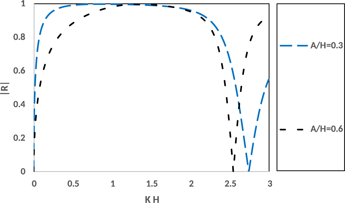
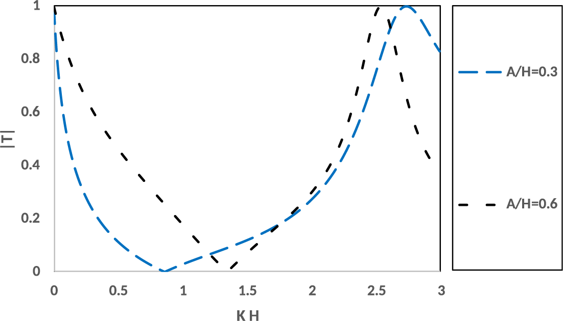
Figures 7 and 8 illustrate the effect of a submerged length of a rectangular box of the
 $\large \boldsymbol \sqcap $
-shaped breakwater on the reflection coefficient and transmission coefficients. Here,
 $|R|,~|T|$
are plotted against the nondimensional wavenumber
 $KH$
for two different draughts of rectangular
 $\large \boldsymbol \sqcap $
-shaped breakwater
 $(A/H = 0.3,~0.6)$
and fixed values of
 $B/H=0.3, ~D/H=0.8,~L/H=1.3, ~h/H=1.3$
.
 $|R|$
against
 $KH$
for
 $B/H=0.3, ~D/H=0.8,~L/H=1.3, ~h/H=1.3$
, for various
 $A/H$
.

 $|T|$
against
 $KH$
for
 $B/H=0.3,~D/H=0.8,~L/H=1.3, ~h/H=1.3$
, for various
 $A/H$
.

From these figures, it is observed that
 $|R|,~|T|$
exhibit oscillatory behaviour for various values of
 $A/H$
and, for certain values of wavenumber
 $KH$
,
 $|R|$
vanishes and
 $|T|$
becomes unity as is evident from Figure 7. Also, Figure 8 shows that
 $|T|$
vanishes and
 $|R|$
becomes unity for certain values of
 $KH$
. It is also observed that as
 $A/H$
increases, a phase shift occurs in oscillations of
 $|R|$
and
 $|T|$
. The zeros of
 $|R|$
shift to the left and the zeros of
 $|T|$
shift to the right as
 $A/H$
increases.
4.5 Effect of width of the trench and the width of the breakwater
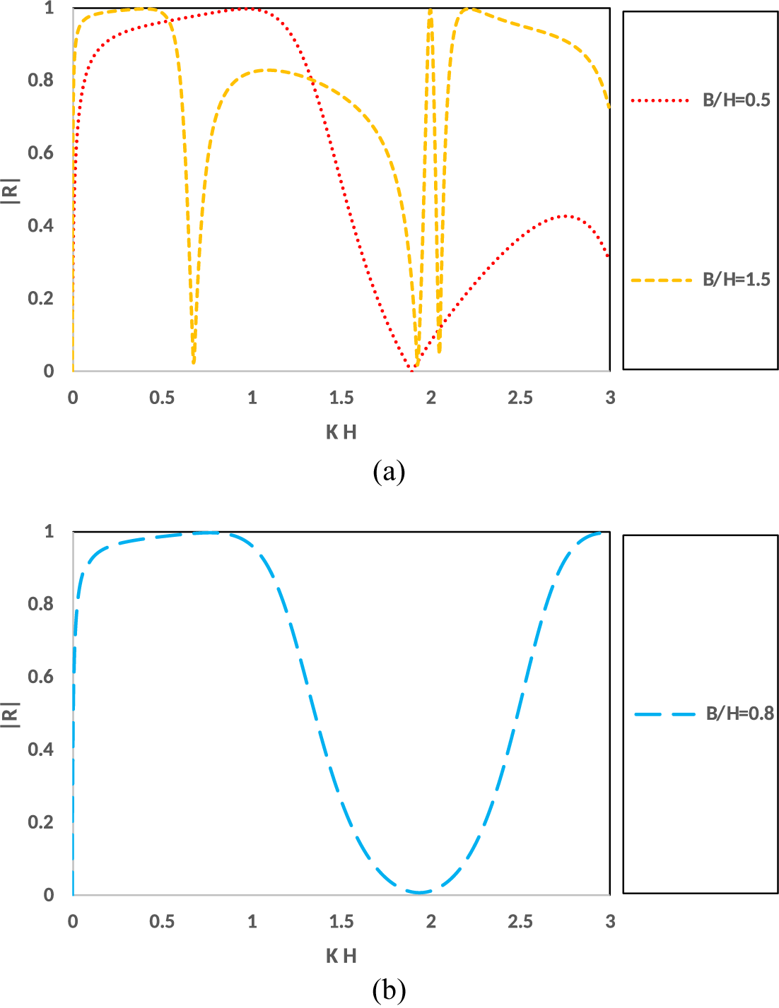
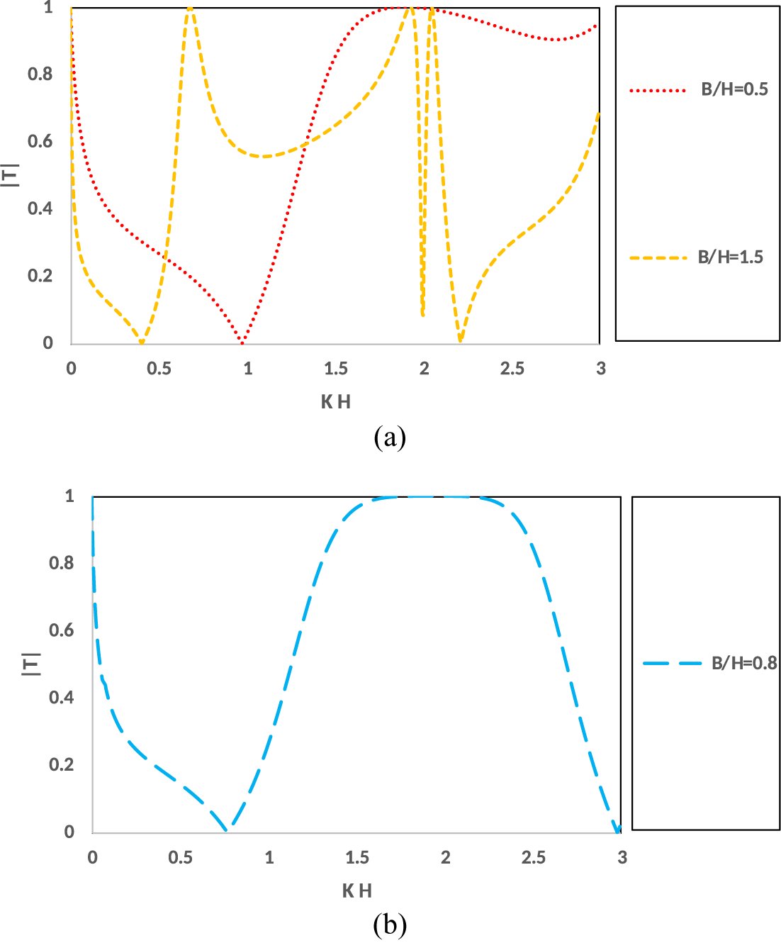
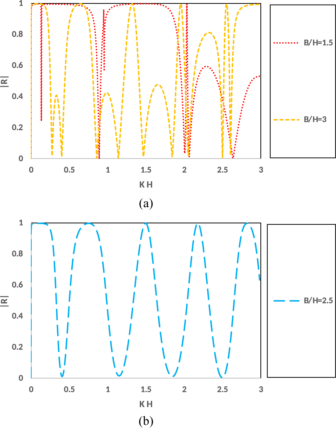
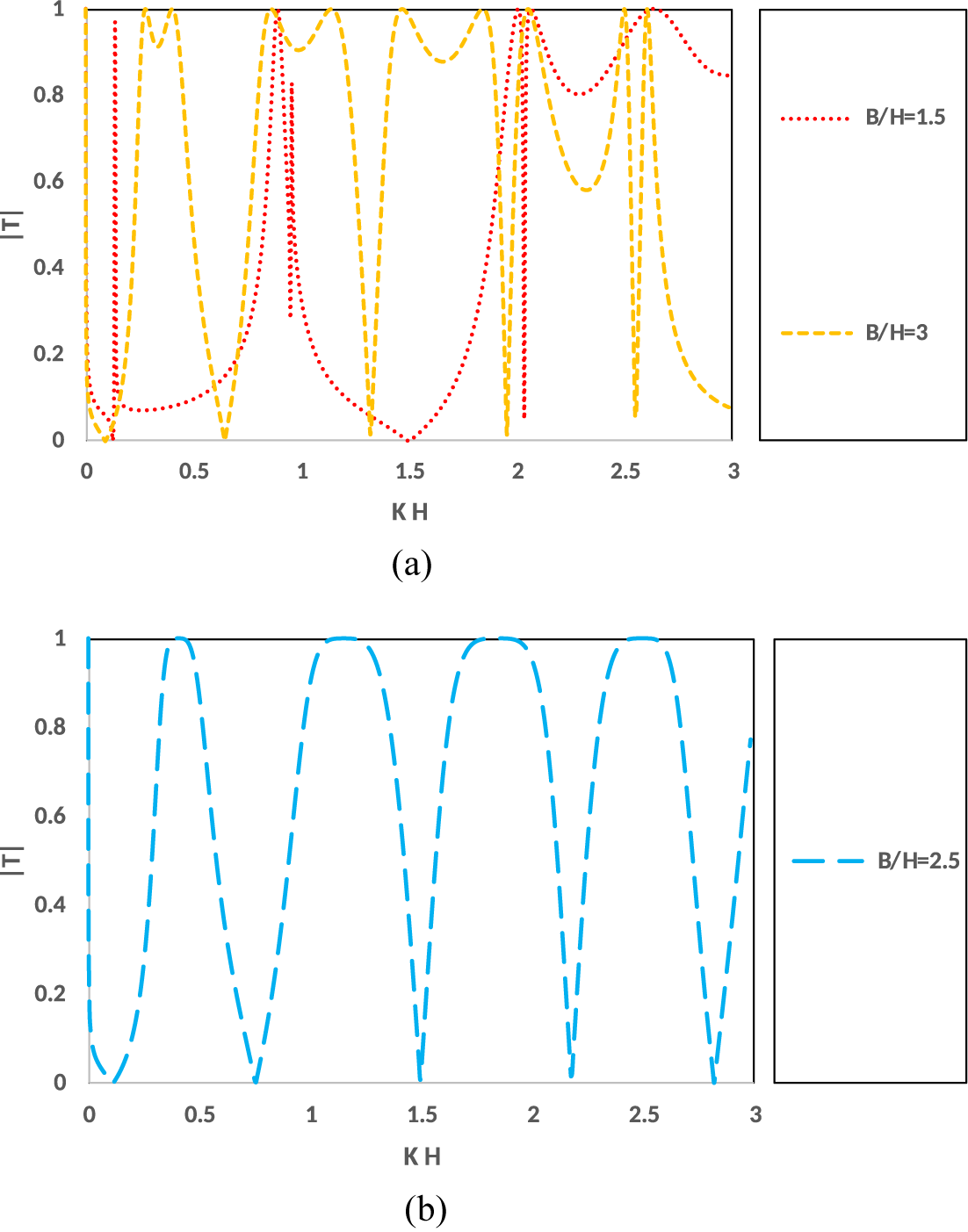
Figures 9(a)–12(b) illustrate the effect of the width of the trench and that of the breakwater on
 $|R|$
and
 $|T|$
.
 $|R|$
against
 $KH$
for
 $A/H=0.25, ~D/H=0.45,~L/H=0.8, ~h/H=1.2$
, for various
 $B/H$
.

Figures 9(a)–10(b) depict
 $|R|$
and
 $|T|$
against the wavenumber
 $KH$
for different widths of the breakwater
 $B/H= 0.5,\, 0.8,\, 1.5$
when the width of the trench is
 ${L/H=0.8}$
and
 $A/H=0.25,~ D/H=0.45,~ h/H=1.2$
.
 $|T|$
against
 $KH$
for
 $A/H=0.25, ~D/H=0.45,~L/H=0.8, ~h/H=1.2$
, for various
 $B/H$
.

Figures 11(a) and 12(b) depict
 $|R|$
and
 $|T|$
against the wavenumber
 $KH$
for various widths of the breakwater
 $B/H= 1.5,~ 2.5,~ 3.0$
when the width of the trench is
 ${L/H= 2.5}$
and
 $A/H=0.25,~ D/H=0.45,~ h/H=1.2$
.
 $|R|$
against
 $KH$
for
 $A/H=0.25, ~D/H=0.45,~L/H=2.5, ~h/H=1.2$
, for various
 $B/H$
.

 $|T|$
against
 $KH$
for
 $A/H=0.25, ~D/H=0.45,~L/H=2.5, ~h/H=1.2$
, for various
 $B/H$
.

We may mention here that Figures 9(b), 10(b), 11(b) and 12(b) depict
 $|R|$
and
 $|T|$
when the width of the breakwater is equal to the width of the trench. It may be noted here that when the width of the trench is equal to the width of the breakwater, that is, when
 $B=L$
, then Regions
 $R2$
and
 $R3$
coincide and in the boundary value problem (2.1)–(2.10), B is replaced by L in (2.1)–(2.3), (2.6)–(2.10) and the conditions (2.4)–(2.5) modify to
 $$ \begin{align*} \phi_x=0 \quad \text{on~} x=\pm L,~0<y<D\quad \text{in Region R1, L1,} \end{align*} $$
 $$ \begin{align*} \phi_x=0 \quad \text{on~} x=\pm L,~A<y<D\quad \text{in Region R2, L2,} \end{align*} $$
conditions on the horizontal side of the breakwater to
 $$ \begin{align*} \phi_y=0 \quad \text{on~} y=A,~-L<x<L \quad \text{in Region R2, L2.} \end{align*} $$
A schematic diagram for when
 $B=L$
is given in Figure 13.
Subregions of the fluid domain when
 $B=L$
.

From Figures 9(a)–12(b), the following observations are made.
(i) When the width of the breakwater is equal to the width of the trench
 ${(B/H=L/H)}$
,
 $|R|$
and
 $|T|$
show uniform smooth oscillations as is evident from Figures 9(b), 10(b), 11(b) and 12(b). The frequency of oscillation is more for a wide trench
 $L/H= 2.5$
than a short trench
 $L/H= 0.8$
.
(ii) For a short trench, when the width of the breakwater is less than the width of the trench,
 $(B/H=0.5,~L/H=0.8)$
,
 $|R|$
and
 $|T|$
show nonuniform oscillations with
 $|R|$
vanishing and
 $|T|$
becoming unity at
 $KH \simeq 1.8$
, and
 $|T|$
vanishing and
 $|R|$
becoming unity at
 $KH \simeq 1.0$
. For
 $KH>1.8,$
the amplitude of oscillation of
 $|R|$
decreases as
 $KH$
increases.
However, when the width of the breakwater is more than the width of the trench
 $(B/H=1.5,~L/H=0.8)$
,
 $|R|$
and
 $|T|$
show nonuniform oscillations and a resonating behaviour in
 $|R|$
is observed for
 $KH \simeq 1.8$
.
(iii) For a wide trench, when the width of the breakwater is less than the width of the trench
 $(B/H=1.5,~L/H=2.5)$
,
 $|R|$
and
 $|T|$
show nonuniform oscillations with
 $|R|$
vanishing sharply at
 $KH \simeq 0.8$
and a resonating behaviour in
 $|R|$
is observed for
 $KH \simeq 2.0$
. However, when the width of the breakwater is more than the width of the trench
 $(B/H=3.0,~L/H=2.5)$
,
 $|R|$
and
 $|T|$
show nonuniform oscillations and, in this case, the frequency of oscillations is more than in the case when the width of the breakwater is less than the width of the trench.
Thus, when the width of the trench is equal to the width of the breakwater, the waves interact uniformly with the trench and the breakwater producing smooth uniform oscillations in the reflected and transmitted waves. However, when the width of the trench and the width of the breakwater are unequal, nonuniform, nonsmooth oscillations in the reflected and transmitted waves are observed and, in some cases, a resonance in the reflected wave is observed. These phenomena occur due to the interaction of waves with the trench and the breakwater.
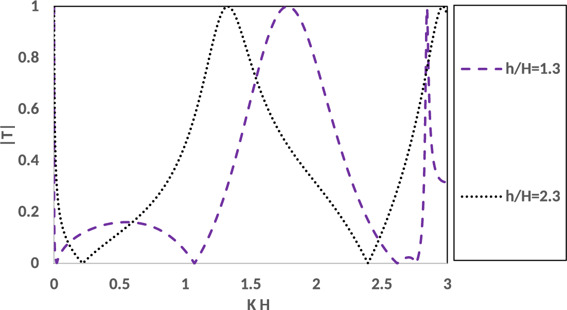
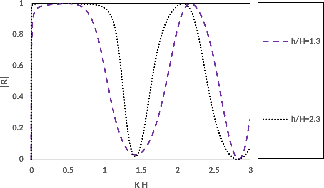
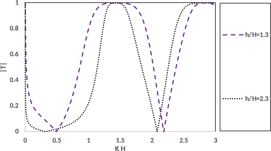
(iv) For a trench with a particular width, it is observed that the frequency of oscillations increases with the increase of width of the breakwater. This is due to the fact that as the width of the breakwater increases, more interaction of waves with the breakwater and the nonuniform bottom occurs which results in increasing the frequency of oscillations in the reflected and transmitted waves.
4.6 Effect of depth of the trench
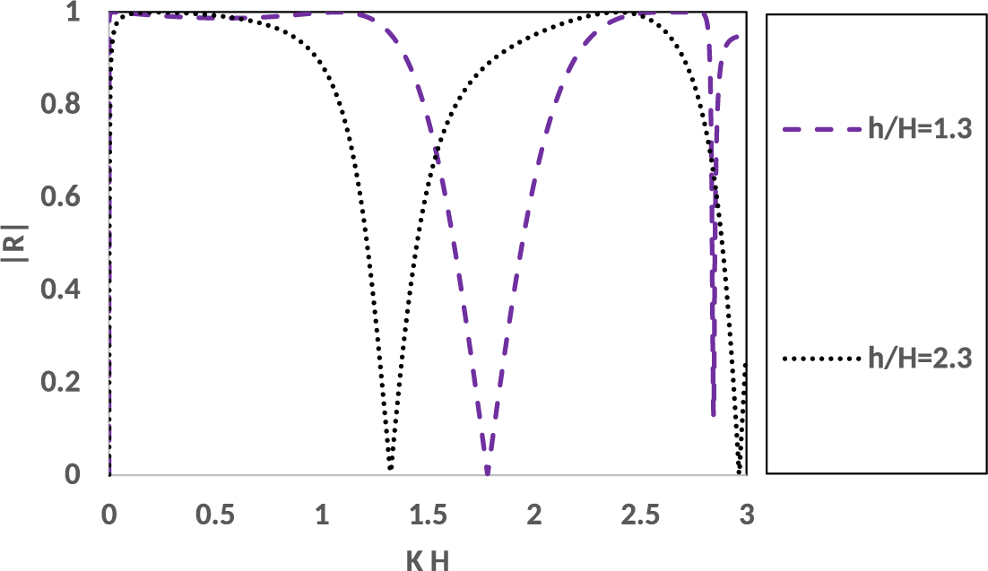
Figures 14 and 15 illustrate the effect of the depth of the trench on the reflection and transmission coefficients. Here,
 $|R|,~|T|$
are depicted against the nondimensional wavenumber
 $KH$
for various values of
 $h/H$
, that is,
 $(h/H = 1.3,~2.3)$
and for fixed values of
 $A/H=0.4, ~B/H=0.4,~D/H=0.6, L/H=1.1$
. From the figures, it is observed that when the width of the breakwater is less than the width of the trench,
 $|R|$
and
 $|T|$
show nonuniform oscillatory behaviour. However, when the width of the breakwater is equal to the width of the trench
 $(L/H=B/H=1.1)$
,
 $|R|$
and
 $|T|$
show uniform oscillatory behaviour as is evident from Figures 16 and 17. Thus, it is seen that the impact of the breakwater and the trench, when the width of the breakwater is equal to the width of the trench, produces uniform oscillations on the reflected and transmitted waves rather than when the width of the breakwater is not equal to the width of the trench.
 $|R|$
against
 $KH$
for
 $A/H=0.4, ~B/H=0.4,~D/H=0.6, ~L/H=1.1$
, for various
 $h/H$
.

 $|T|$
against
 $KH$
for
 $A/H=0.4, ~B/H=0.4,~D/H=0.6, ~L/H=1.1$
, for various
 $h/H$
.

 $|R|$
against
 $KH$
for
 $A/H=0.4, ~B/H=1.1,~D/H=0.6, ~L/H=1.1$
, for various
 $h/H$
.

 $|T|$
against
 $KH$
for
 $A/H=0.4, ~B/H=1.1,~D/H=0.6, ~L/H=1.1$
, for various
 $h/H$
.

4.7 Effect of trench on the reflection and transmission coefficients
If we compare the behaviour of
 $|R|$
and
 $|T|$
due to
 $\large \boldsymbol \sqcap $
-shaped breakwater present in water of uniform finite depth as studied by Singh et al. [Reference Singh, Kaligatla and Mandal20] with that due to the presence of a trench as analysed in the present study, it is found that the presence of a trench produces oscillatory behaviour in the reflection and transmission coefficients, and for certain values of wavenumber, the phenomena of total reflection, zero transmission or total transmission and zero reflection occur. Thus, we can infer that the phenomenon of water wave scattering by a
 $\large \boldsymbol \sqcap $
-shaped breakwater in the presence of a trench produces oscillations in the reflection and transmission coefficients which is in contrast with the behaviour of reflection and transmission coefficients in the absence of a trench as observed in [Reference Singh, Kaligatla and Mandal20].
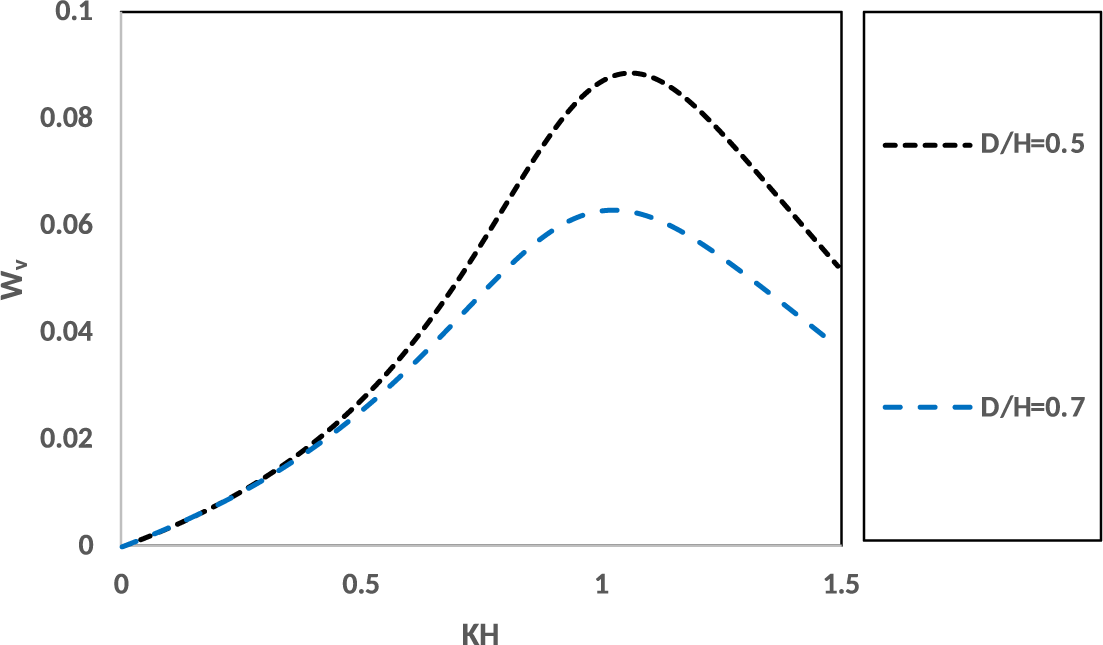
4.8 Horizontal and vertical forces on the breakwater
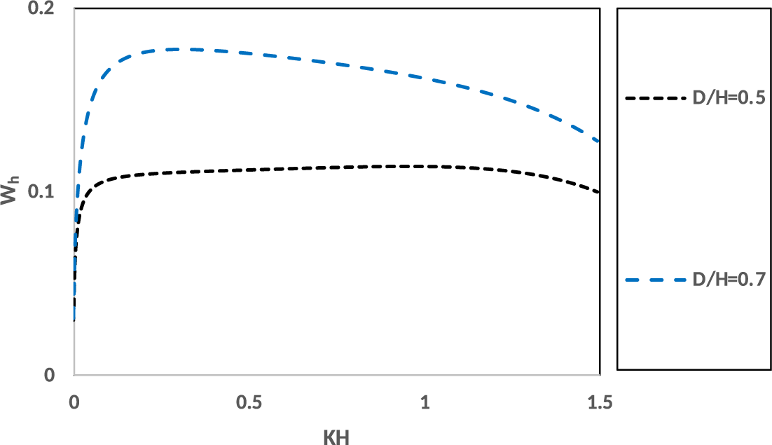
Figures 18 and 19 illustrate the effect of the length of the side wall (
 $D/H$
) of the
 $\large \boldsymbol \sqcap $
-shaped breakwater on horizontal force
 $W_{h}$
and vertical force
 $W_{v}$
. Here,
 $W_{h}, ~W_{v}$
are plotted against the nondimensional wavenumber
 $KH$
for two different lengths of the side wall (
 $D/H = 0.5,~ 0.7$
) of the
 $\large \boldsymbol \sqcap $
-shaped breakwater for
 $(A/H = 0.3)$
and fixed values of
 $L/H=1.3, ~B/H=0.8,~h/H=1.3$
.
 $W_{h}$
against
 $KH$
for
 $L/H=1.3, ~B/H=0.8,~A/H=0.3, ~h/H=1.3$
, for various
 $D/H$
.

 $W_{v}$
against
 $KH$
for
 $L/H=1.3, ~B/H=0.8,~A/H=0.3, ~h/H=1.3$
, for various
 $D/H$
.

From Figures 18 and 19, it is observed that for a fixed width of the breakwater, as the length of side wall (
 $D/H$
) of the
 $\large \boldsymbol \sqcap $
-shaped breakwater increases, the horizontal force increases and the vertical force decreases. This is expected because as the length of side wall (
 $D/H$
) of the
 $\large \boldsymbol \sqcap $
-shaped breakwater increases, the impact of incident waves on the side walls of the breakwater increases substantially and so the horizontal force on the breakwater increases.
Kaligatla et al. [Reference Kaligatla, Singh and Mandal10] observed that for obliquely incident waves with angle of incidence as
 $30^\circ $
on a
 $\large \boldsymbol \sqcap $
-shaped breakwater present in deep water, the vertical force on the breakwater is more than the horizontal force. Also, they showed that the forces decrease with an increase of the width of the breakwater.
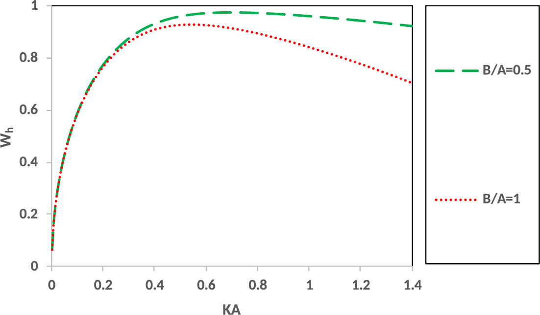
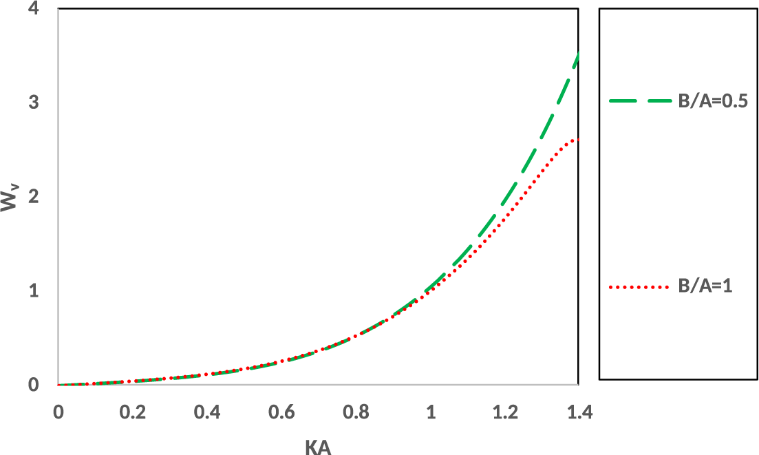
In the present study, in Figures 20 and 21, the horizontal and vertical forces
 $W_{h},W_{v}$
are plotted against the nondimensional wavenumber
 $KA$
for two different widths of the breakwater
 $B/A (=0.5,1)$
and for a normally incident wave train on the
 $\large \boldsymbol \sqcap $
-shaped breakwater present in deep water
 $H/A=h/A=4$
in the absence of a trench (
 ${L/A=0.001}$
).
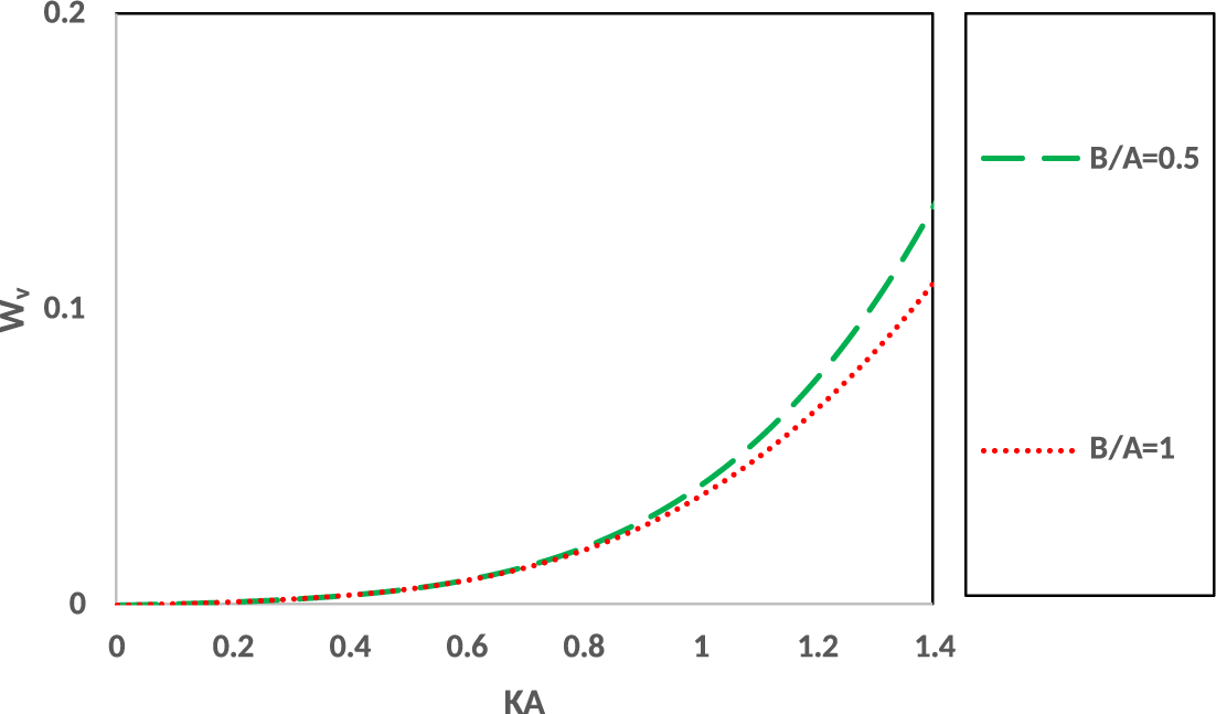
 $W_{h}$
against
 $KA$
for
 $L/A=0.001, ~D/A=2,~H/A=4, ~h/A=4$
, for various
 $B/A$
.

 $W_{v}$
against
 $KH$
for
 $L/A=0.001, ~D/A=2,~H/A=4, ~h/A=4$
, for various
 $B/A$
.

Here, in the absence of a trench, when the water region is deep (
 $H/A=h/A=4$
), it is observed that for a fixed width of the breakwater, the vertical force is more than the horizontal force and this is significant for higher wavenumber. This phenomenon is similar to that observed by Kaligatla et al. [Reference Kaligatla, Singh and Mandal10, Figure 9] when the angle of incidence is
 $30^\circ $
. However, this behaviour of the forces depicted in Figures 20 and 21 is in contrast with the behaviour of the forces exerted on
 $\large \boldsymbol \sqcap $
-shaped breakwater present in the water region with a trench (see Figures 18 and 19) where the horizontal force exerted on the breakwater is more than the vertical force for any length of the side wall of the breakwater. This change in the behaviour of the forces illustrates the effect of the depth of the water region. For a uniformly deep water region, the large water column below the breakwater exerts a pressure force below the breakwater vertically. Due to this reason, the vertical force exceeds the horizontal force when the water is deep.
Thus, we can conclude from Figures 18–21 that due to presence of a trench: (1) the horizontal force increases and vertical force decreases with the increase in length of the side wall of the
 $\large \boldsymbol \sqcap $
-shaped breakwater; and (2) for a fixed dimension of the breakwater, when the bottom of the water region has nonuniform bathymetry (that is, the presence of a trench), the horizontal force is more than the vertical force. However, in the absence of a trench, when a
 $\large \boldsymbol \sqcap $
-shaped breakwater is present in uniformly deep water, the vertical force exerted on the breakwater is more than the horizontal force.
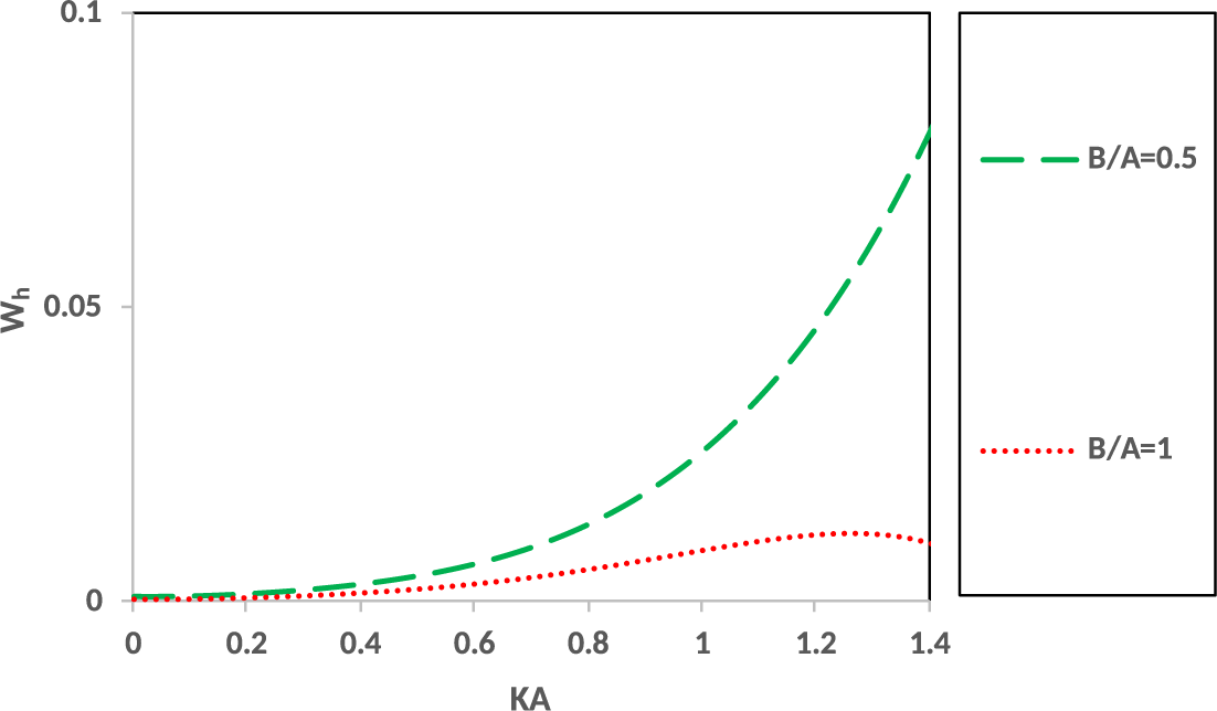
Figures 22 and 23 illustrate the horizontal and vertical forces exerted on the breakwater without the legs, that is, the
 $\large \boldsymbol \sqcap $
-shaped breakwater takes the shape of a rectangular box. From these figures, it is seen that for a rectangular breakwater present in uniformly deep water (without any trench), the horizontal force is less than the vertical force. This is also due to the reason that for deep water, the long column of water below the breakwater exerts a pressure force normally on it. This phenomenon was also observed by Kaligatla [Reference Kaligatla, Singh and Mandal10] when the angle of incidence is
 $30^\circ $
.
 $W_{h}$
against
 $KA$
for
 $L/A=0.001, ~D/A=1,~H/A=4, ~h/A=4$
, for various
 $B/A$
.

 $W_{v}$
against
 $KH$
for
 $L/A=0.001, ~D/A=1,~H/A=4, ~h/A=4$
, for various
 $B/A$
.

4.9 Velocity diagram as time elapses
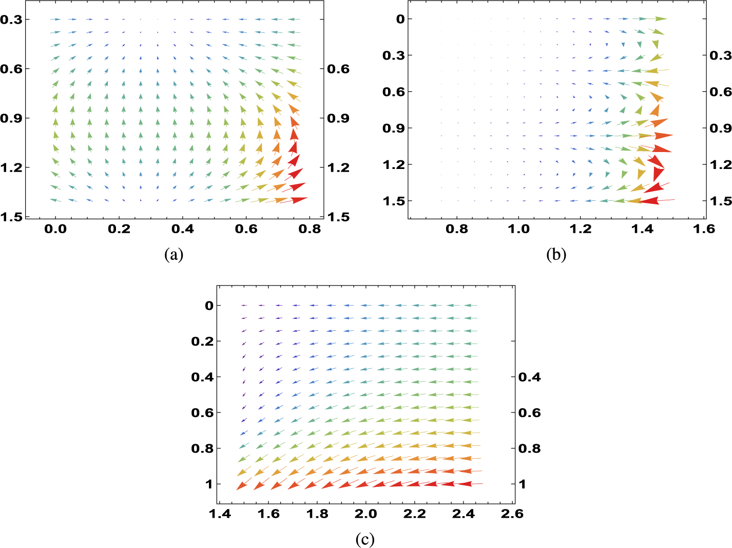
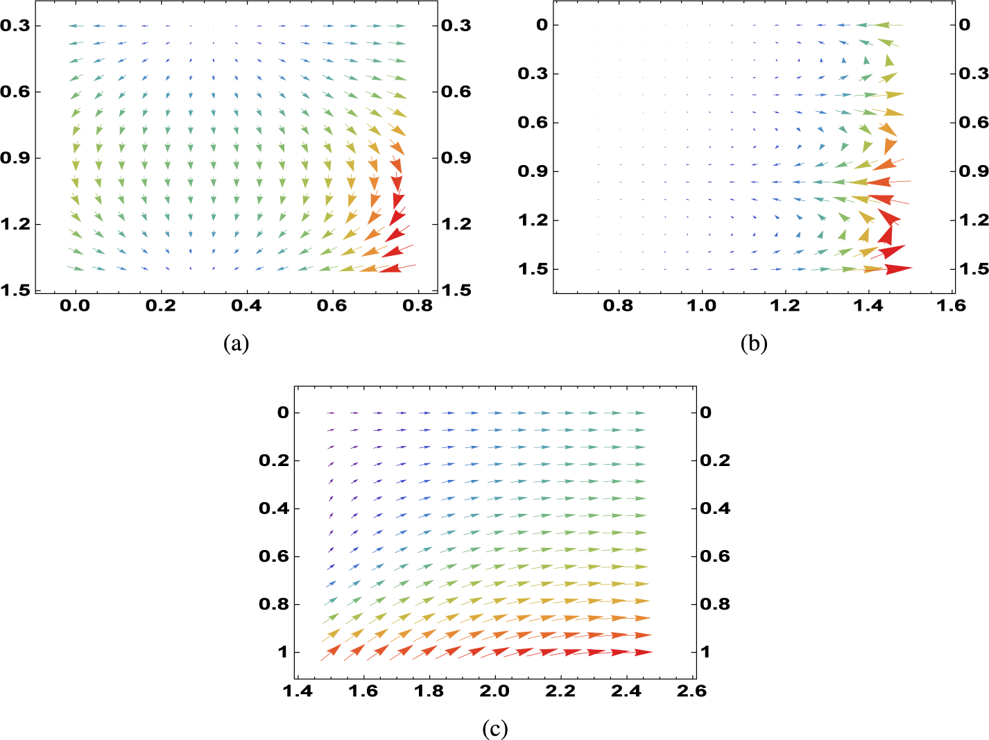
Figures 24(a), 24(b), 24(c) capture the fluid velocity in the
 $(X=x/H,~ Y=y/H)$
plane, just after the motion started, at nondimensional time
 $\omega t=10^{-4}$
, while Figures 25(a), 25(b), 25(c) depict fluid velocity at nondimensional time
 $\omega t=3$
in the Regions R3, R2, R1, respectively, for
 ${A}/{H}=0.3, {D}/{H}=0.8,~ {B}/{H}=0.75,~ {L}/{H}=1.5,~ {h}/{H}=1.5.$
Fluid velocity at time
 $\omega t=10^{-4}$
in (a) Region R3, (b) Region R2, (c) Region R1 when
 ${A}/{H}=0.3,~{D/}{H}=0.8,~{B}/{H}=0.75,~{L}/{H}=1.5,~{h}/{H}=1.5$
.

Fluid velocity at time
 $\omega t=3$
in (a) Region R3, (b) Region R2, (c) Region R1, when
 ${A}/{H}=0.3,~{D}/{H}=0.8,~{B}/{H}=0.75,~{L}/{H}=1.5,~{h}/{H}=1.5$
.

Figures 24(a) and 25(a) represent the fluid velocity at time
 $\omega t=10^{-4},~3$
, respectively, in the Region R3 where R3:
 $0\leq X \leq {B}/{H}=0.75,~ {A}/{H}=0.3\leq Y \leq {h}/{H}=1.5.$
Figures 24(b) and 25(b) represent the fluid velocity at time
 $\omega t=10^{-4},~3$
, respectively, in the Region R2 where R2:
 $0.75\leq X \leq {L}/{H}=1.5,~ 0\leq Y \leq {h}/{H}=1.5.$
Figures 24(c) and 25(c) represent the fluid velocity at time
 $\omega t=10^{-4},~3$
, respectively, in the Region R1 where R1:
 ${L}/{H}\leq X \leq \infty ,~ 0\leq Y \leq {H}/{H}=1.$
4.9.1 Velocity behaviour in Region R3.
Initially, just after the motion started, at
 $\omega t=10^{-4}$
, the incident wave from a large distance encounters the
 $\large \boldsymbol \sqcap $
-shaped breakwater at the interface of regions R3 and R2, and so the direction of velocity is inwards towards the breakwater. We may mention that the sharp end of the leg of the breakwater is at the point
 $({B}/{H},{d}/{H})=(0.75,0.8)$
and by edge condition (2.8), the velocity exhibits singular behaviour at this point. Figure 24(a) shows that fluid velocity is significant for
 $X={B}/{H}=0.75,~0.8\leq Y\leq {h}/{H}$
, and the direction of velocity is upward from the bottom of the trench towards the lower part of the breakwater in two opposite directions moving inwards below the breakwater.
As time progresses, that is, at
 $\omega t=3$
, the waves get reflected by the breakwater and, thus, the direction of velocity is outwards away from the breakwater. Also due to the edge condition (2.8), the velocity is significant in the region
 ${X={B}/{H},~0.8\leq Y\leq {h}/{H}}$
as is observed from Figure 25(a). Also, it is observed from Figure 25(a) that the direction of velocity in this region is from the bottom of the breakwater towards the bottom of the trench moving inwards. This behaviour of the velocity is due to the interaction of fluid with the trench and the tip of the legs of the breakwater.
4.9.2 Velocity behaviour in Region R2.
In this region, just after the motion started, at time
 $\omega t=10^{-4},$
the velocity shows significant behaviour along the wall of the trench and around the corner of the trench. It is to be mentioned that at the corner point
 $({L}/{H}=1.5,1)$
of the trench, the velocity has singular behaviour as given by condition (2.9). Thus, for
 $X={L}/{H},~1\leq Y \leq {h}/{H}=1.5$
, the velocity is significant in this part. As time elapses, that is, for
 $\omega t=3$
, it is observed from Figure 25(b) that the velocity shows significant behaviour around the corner of the trench and along the wall of the trench, but the direction is opposite to that at the initial time.
4.9.3 Velocity behaviour in Region R1.
Just after the initial moment, at time
 ${\omega t=10^{-4}}$
, due to an incoming wave incident on the breakwater, the direction of velocity is inward towards the breakwater. However, as time elapses, that is, for
 $\omega t=3$
, due to the reflection by the breakwater, the direction of velocity changes and fluid moves outwards towards the infinity. In region R1, due to the corner point of the trench and also due to effect of the bottom, the velocity is significant at the bottom of this region, that is, at
 $Y={H}/{H}=1, {L}/{H}\leq X \leq \infty $
.
5 Conclusion
Scattering of water waves by a
 $\large \boldsymbol \sqcap $
-shaped breakwater in the presence of a rectangular trench is studied by using the integral equation method. The integral equations are solved by the Galerkin approximation method in terms of Chebyshev and Gegenbauer polynomials. The choice of polynomials depends on the behaviour of the functions satisfying the integral equation at the edges of the breakwater and the trench. Using the solutions of the integral equations, the reflection and transmission coefficients, and the forces on the breakwater are evaluated and depicted graphically for various values of the parameters. The convergence of the Galerkin method is shown in tabular form. The results obtained in the present study are compared with the known results in the literature to validate the authenticity of the methodology used. From the graphical results, the following observations are made.
(i) The figures illustrating the reflection and transmission coefficients in the presence of a trench obtained in the present study are compared with those in the absence of a trench, available in the literature. The present study shows that the presence of a trench produces oscillatory behaviour in the reflected and transmitted waves due to a
 $\large \boldsymbol \sqcap $
-shaped breakwater as compared with those in the absence of a trench.
(ii) When the width of the trench is equal to the width of the breakwater, the waves interact uniformly with the trench and the breakwater producing smooth uniform oscillations in the reflected and transmitted waves. However, when the width of the trench and the width of the breakwater are unequal, nonuniform, nonsmooth oscillations in the reflected and transmitted waves are observed and, in some cases, a resonance in the reflected wave is observed. This phenomenon occurs due to the interaction of waves with the trench and the breakwater.
(iii) For a trench with a particular width, it is observed that the frequency of oscillations increases with the increase of the width of the breakwater which is due to the fact that as the width of the breakwater increases, more interaction of waves with the breakwater and the nonuniform bottom occurs.
(iv) It is also observed that the horizontal force exerted on the breakwater increases and the vertical force decreases as the length of the side wall of the
 $\large \boldsymbol \sqcap $
-shaped breakwater increases. This is because as the length of side wall (
 $D/H$
) of the
 $\large \boldsymbol \sqcap $
-shaped breakwater increases, the impact of incident waves on the side walls of the breakwater increases substantially and so the horizontal force on the breakwater increases.
(v) Also, for a fixed dimension of the breakwater, the horizontal force is more than the vertical force.
(vi) In the absence of a trench, for a
 $\large \boldsymbol \sqcap $
-shaped breakwater present in deep water, the vertical force exerted on the breakwater is more than the horizontal force. Also, this observation is also noted when the rectangular box shaped breakwater is present in deep water. This behaviour was also observed by Kaligatla et al. [Reference Kaligatla, Singh and Mandal10]. This happens for deep water where the large column of water exerts a normal pressure force on the breakwater. However, for finite depth water, with a trench, the contrast behaviour, where the horizontal force is more than the vertical force, is observed.
(vii) The velocity plot illustrates the behaviour of the fluid velocity in the fluid region at initial time and as time elapses. These diagrams show that there is a change in the direction of the fluid velocity with the progress of time and the velocity is significant near the sharp end of the breakwater as well as near the corner of the trench.
Acknowledgements
This work is partially supported by the National Natural Science Foundation of China (Nos. W2433140, 52350410468, W2541018) through Gour Das, and is also partially supported by the State Government Departmental Fellowship Scheme (Ref. No.: P-1/Rs/34/25) through Shreya Banerjee.