1. Introduction
In recent years, more and more environmental conflicts between provinces have been attracting great attention in China. For example, in January 2008 residents of the Wuqing district (Tianjin province) complained that a cement plant in the neighboring Xianghe county (Hebei province) had over-discharged dust pollution which then crossed the province border and damaged their soil and crop production (Wuqing District Environmental Protection Bureau, 2008). Disputes invol-ving the Huai River, which runs through Henan, Shandong, Anhui and Jiangsu provinces, are also very illustrative of ever-increasing transborder conflicts. On several occasions, downstream provinces have accused upstream provinces of dumping pollution into the river in order to evacuate it to other provinces. As polluters from a given province can evacuate a part of their pollution to other provinces, there is a risk of excess of pollution at regional borders of the countries.
There is already quite strong evidence that a decentralized environmental policy can lead to pollution havens and free-riding effects, resulting in an excess of pollution at regional borders. This is what is known as transboundary pollution. Transboundary pollution is a very serious problem as it appears that people in border counties suffer disproportionate health problems as a result of pollution. Indeed, in the United States, cancer rates are substantially higher in border counties than in interior ones due to transboundary pollution (Kahn, Reference Kahn2004). Until now, almost all studies have been focused on the United States (Helland and Whitford, Reference Helland and Whitford2003; Kahn, Reference Kahn2004; Sigman, Reference Sigman2002; Konisky and Woods, Reference Konisky and Woods2010). Very few have looked at this issue in emerging countries. Lipscomb and Mobarak (Reference Lipscomb and Mobarak2007) constitute one exception, with their analysis of water pollution spillovers in Brazil.
China meets all the conditions that make it susceptible to the emergence of transboundary pollution. Indeed, China's environmental policy is decentralized: while the central government sets environmental standards, it is the local governments who monitor and impose sanctions on polluters. In the Chinese context, as we will see in more detail in section 3, there is a high probability for the existence of free-riding and pollution havens. In addition, environmental conflicts between provinces provide some evidence that transboundary pollution is already occurring. However, until now, transboundary pollution in China has not received the attention it deserves, primarily due to the lack of available data.
This study contributes to the literature by studying whether or not transboundary pollution does indeed exist in China today. To address this question, we study the location choice of polluting firms between 2002 and 2008 in Hebei, one of the most highly polluted provinces in the country. Specifically, we test whether polluting firms are more likely to set up in countiesFootnote 1 that share a border with another province than in interior counties. For this purpose, we use the lists of polluting firms published annually by the Ministry of Environmental Protection (MEP) and by the Environmental Protection Bureau (EPB) of Hebei Province. To ensure the robustness of our results, several measures of the variable of interest have been constructed from Geographic Information System (GIS) data. We find very robust evidence, even after controlling for confounding factors such as market access, that border counties are more attractive destinations for polluting firms than interior counties. Moreover, it appears that this effect has been increasing over time.
By demonstrating that border county residents are more highly exposed to pollution, we also contribute to the very scarce literature on environmental inequality in China. Two notable exceptions are Ma (Reference Ma2010) and Schoolman and Ma (Reference Schoolman and Ma2011), who investigate how socio-economic characteristics of townships influence the geographic repartition of pollution. Ma (Reference Ma2010) highlights that rural residents, and especially rural migrants, suffer disproportionately from pollution in Henan. Schoolman and Ma (Reference Schoolman and Ma2011) emphasize that migrants are disproportionately exposed to pollution in Jiangsu and put forward a general theory of environmental inequality by highlighting that in China, as in the US, individuals at the bottom of the social ladder bear most of the environmental burden. By proposing an additional lens (proximity to regional borders) to analyze environmental inequality, the present study provides complementary results to these previous works.
The remainder of the article is organized as follows. Following the introduction, in section 2 we briefly present China's environmental policy. Next, we study why, in the context of a decentralized policy, polluting firms would tend to agglomerate near regional borders. Section 4 describes the study area and the data. We present the estimation strategy in section 5 and the results in section 6. Finally, we conclude and offer some policy recommendations.
2. Environmental policy in China
2.1. A decentralized environmental policy
During the 1980s China's environmental policy followed the general trend of decentralization occurring in the country and since then its enforcement has depended largely on local governments. Environmental protection is currently managed at the national level by the MEP and, at the regional and local levels (provinces, prefectures and counties), by the EPBs. The central government establishes environmental standards whereas environmental policy is implemented by the regions which monitor emissions and impose penalties if standards are not met. Decentralization of environmental policy in a country as heterogeneous as China offers undeniable advantages. Indeed, it allows for greater flexibility as well as better information and adaptation to the local context. However, as local officials are evaluated more on economic than on environmental performance, environment protection is often sacrificed for economic gain, resulting in significant environmental degradations.
Facing this critical situation, a certain ‘recentralization’ of China's environmental policy has occurred. In 2008, the State Environmental Protection Agency (SEPA) became the MEP in order to give more power back to the central government. Moreover, between 2006 and 2008, six major supervision centers were created. Each of these major centers is responsible for several provinces and monitors whether or not they respect the environmental standards established by the central government. These centers are also in charge of coordinating interprovincial conflicts. Thus, they constitute a new intermediary level between central government and provinces, established with the aim of limiting the negative effects of decentralization. However, until now, the power of these new centers has been very limited and environmental policy is still largely implemented by Chinese provinces.
2.2. Impact of environmental regulations on polluting firms
Like all firms, those that pollute do not choose their location randomly; they decide to locate in a particular region to maximize their profit. Several studies show that in China the location choice of both foreign (Wu, Reference Wu1999) and Chinese firms (Wen, Reference Wen2004) depends today on ‘rational economic considerations’. Thus, firms are generally attracted to regions with good market opportunities and where labor is cheap and skilled.
Polluting firms, in addition, usually take into account the severity of environmental regulation when deciding where to set up. This is likely to be the case in China, where it has been shown that environmental regulations significantly raise the costs of polluting firms. For example, Wang (Reference Wang2002) estimates that pollution charges lead to a significant increase in expenditures on end-of-pipe water treatment facilities at the plant level. Moreover, a higher number of inspections leads to a higher expected penalty for firms that do not comply with environmental standards and, thus, significantly reduces the level of water and air pollution of industries in the city of Zhenjiang (Dasgupta et al., Reference Dasgupta, Laplante, Mamingi and Wang2001). In addition, although state-owned enterprises have more bargaining power with local authorities in terms of the charges they pay (Wang and Wheeler, Reference Wang and Wheeler2005), environmental policy also has a significant impact on them (Wang et al., Reference Wang, Mamingi, Laplante and Dasgupta2003). As a consequence, given that environmental regulation in China imposes significant costs on polluting firms, we would expect these firms to locate in regions with less stringent environmental regulation.
3. Literature review: why would polluting firms be more likely to set up near borders?
As explained in section 2.2., polluting firms are expected to set up in regions with less stringent environmental regulations. In this section, we explain how regional differences in environmental regulations lead polluting firms to set up more frequently in border counties. Specifically, two phenomena could lead to transboundary pollution, namely ‘pollution havens’ and ‘free-riding’ effects.
3.1. Differences in interprovincial regulation: pollution havens hypothesis at the provincial level
In China, environmental policy implementation varies greatly from one province to another (Wang et al., Reference Wang, Mamingi, Laplante and Dasgupta2003). Such disparity in policy enforcement by region would be at the origin of a ‘pollution havens’ phenomenon at the provincial levelFootnote 2: polluting firms would be attracted to provinces where environmental regulations are less strict (Dean et al., Reference Dean, Lovely and Wang2009). Indeed, at the borders, there are discontinuities in environmental regulations (Kahn, Reference Kahn2004). By crossing an administrative boundary, one can suddenly move from strict environmental regulation to a less restrictive one. In this context, it could be very profitable for a firm to locate on the border between two provinces. Crossing a border can therefore be a way to avoid stringent environmental regulations while continuing to benefit from the market access of the neighboring province with stricter environmental regulation. Kahn (Reference Kahn2004) shows that in the United States, in low environmental regulation states, ‘dirty’ industries set up more often in counties that border high-regulation states than in interior counties. Conversely, in counties bordering low-regulation states, there is a lower number of polluting firms. In terms of environmental regulation, Hebei is less stringent than its neighbors, with the exception of Inner Mongolia.Footnote 3 Thus, on the whole, we can expect the pollution havens effect to be positive in Hebei province, leading polluting firms to concentrate close to borders.
3.2. Differences in intra-provincial regulations: free-riding and intra-provincial pollution havens hypotheses
When environmental policy is decentralized, provincial regulators may be less strict in implementing the policy in border counties than in interior ones. In other words, free-riding may emerge at the boundaries between different regions of the country.Footnote 4 Two factors could encourage regulators to strategically implement environmental regulation, both leading to an excess of pollution at borders. First of all, at borders, a region's expenditure on pollution control does not solely benefit that region; it also benefits neighboring ones (Sigman, Reference Sigman2002). Since regions have limited financial resources, they prefer investing funds where they can reap the highest benefit, that is to say, in interior counties. Secondly, at borders, some of a given firm's pollution impacts the neighboring region. Thus, in border counties, the population benefits from the overall positive economic advantages related to the presence of the firm (jobs and taxes) and only suffers from part of the pollution generated (Helland and Whitford, Reference Helland and Whitford2003). On the contrary, in interior counties, the population benefits from job opportunities but must also bear all the pollution generated. Thus, we would expect social discontent related to the establishment of a polluting firm to be higher in interior counties. As a result, a regulator concerned with political supportFootnote 5 and job promotionFootnote 6 will be more likely to oppose the arrival of a polluting firm and to apply more stringent environmental regulations in interior counties. The same free-riding argument applies to coastal counties, explaining why emissions are much higher in these counties (Helland and Whitford, Reference Helland and Whitford2003). It is worth noting that the free-riding effect will always lead polluting firms to concentrate in border counties, whatever the relative stringency of Hebei's environmental regulation. However, the magnitude of the effect is reduced when the neighboring state enforces stringent environmental regulations (Gray and Shadbegian, Reference Gray and Shadbegian2004).
Finally, the strategic implementation of environmental regulation (less stringent regulation at borders) can also lead to an intra-provincial pollution havens effect. Because of their less stringent regulation, we would expect border counties to attract more polluting firms than interior borders, leading to transboundary pollution.
4. Description of the study area and data
4.1. Hebei province
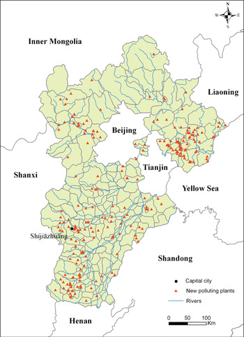
This study is carried out in Hebei Province for several reasons. First of all, Hebei has been industrialized for many decades, which makes it one of the most polluted provinces in the country. According to the list published in 2010 by the Chinese government, which identifies the most polluting firms in China, 744 of the 9,833 top polluters in China are located in Hebei. The province has the highest number of polluting firms just after Jiangsu (838) and Shandong (774). Moreover, Hebei shares borders with seven other provinces including the provincial cities of Beijing and Tianjin (see figure 1). In addition, Hebei has already been involved in several transboundary pollution conflicts, as stated in the introduction. Finally, Hebei is one of the few provinces with the necessary data available to allow us to carry out our study.
Polluting firm births in Hebei province from 2002 to 2008

Regarding environmental protection, environmental policy in Hebei province has been continuously tightened since the beginning of the 2000s.Footnote 7 Thus, we can expect polluting firms to be increasingly sensitive to environmental regulation over the period under study. As discussed in section 6.4, this may have led polluting firms to increasingly settle close to borders over the past few years.
4.2. Construction of the dependent variable and sample
The dependent variable of our model is the annual number of polluting firms set up by county. We constructed this variable from the lists published by the MEP and the EPB of Hebei.Footnote 8 Since 2007, the MEP and EPBs of provinces annually publish lists (Guojia/Sheng zhongdian jiankong qiye mingdan) that identify the most polluting firms in China.Footnote 9 These lists give the name of each firm and the county in which it is located. Moreover, the lists classify each firm as: ‘water polluting firm’, ‘air polluting firm’ or ‘wastewater treatment facility’. Wastewater treatment facilities are always built close to population centers in order to treat municipal waste. As they do not freely choose their location, transboundary pollution is not likely to occur in this case, and therefore we have excluded them from our analysis. By contrast, both air and water pollutant firms freely choose their location and, thus, take into account environmental regulation when deciding where to set up. Thus, we consider both air and water polluting firms when constructing our dependent variable.
However, the MEP and EPBs lists provide no information regarding a firm's establishment date or emissions level. So, these lists give the necessary information to estimate a model of stock, in which the total number of firms in a county is regressed on a set of regional variables. However, in this study we estimate a flow model in which the number of firms created in a county at year t is regressed on the characteristics of this county at year t. Indeed, as there was no environmental policy in China before 1979, to test the existence of transboundary pollution, we were obliged to take a sample of firms which have been recently created and which are, therefore, sensitive to environmental regulation. In addition, the flow model enables us to test whether transboundary pollution has increased over time. In order to estimate a flow model, we have collected the creation dates of polluting firms from the official website of the Industrial and Commercial Bureau of Hebei province.
Once the creation dates were obtained, we selected firms set up after 2002, a year from which we have data for the explanatory variables. In addition, the last list of polluting firms was published in 2010; it lists the most polluting firms in 2008. Thus, our sample covers the period of 2002–2008. In all, 253 air and water polluting firms were set up in Hebei province between 2002 and 2008.
4.3. Variables of interest
Three variables of interest have been constructed to ensure robustness. Firstly, we follow the literature (Helland and Whitford, Reference Helland and Whitford2003; Kahn, Reference Kahn2004; Konisky and Woods, Reference Konisky and Woods2010) and construct a dummy variable equal to 1 if the county shares a border with another province, or the sea, and 0 otherwise (Border_1). As explained in section 3.2, the same free-riding phenomenon is expected to take place in coastal counties. Thus, to capture the whole transboundary pollution effect, we first create a variable including both coastal and other border counties. However, as can be seen in figure 1, some border counties share a very small part of their border with another province while others share more than half of the total length of their border with another province. To take into account the variability among border counties, we create a second variable equal to the length of the common border with another province (or the sea) divided by the total length of the county's border (Border_2). The drawback of the first two variables is that they do not take into account the variability between non-border counties; while some counties are located at the center of the province, others are very close to the borders. Moreover, both measures are likely to be significantly affected by the shape of the county. For these reasons, we create a third variable equal to the distance between the county seat and the closest border (Distance).Footnote 10 These variables have been constructed with GIS data, using ArcGis 9.2. If transboundary pollution exists, we expect polluting firms to be more likely to set up near borders. Therefore, we would expect the coefficients associated with variables Border_1 and Border_2 to be positive and the coefficient associated with ‘Distance’ to be negative.
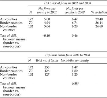
Table 1 gives descriptive statistics on the polluting firms in our sample. Panel A of the table gives the average stock of firms in 2001 and 2008 for all counties, border and non-border. Interestingly, non-border counties had a slightly higher number of polluting firms than border counties in 2001 whereas the opposite was true for 2008.
Polluting firms in Hebei province

Note: *Indicates significance at the 10% level.
Panel B of the table gives data on firm births from 2002 to 2008. It clearly indicates that, over the recent period, polluting firms have located significantly more frequently in border counties, which tends to validate the transboundary pollution hypothesis. Moreover, the differences observed in the stock of firms between non-border and border counties reflect an evolution in polluting firms' location choices in China. Among the firms identified in the lists, some were created before the 1980s. At that time, a firm's location decision was not based on economic rationale but rather arose from a strategy aimed at protecting industries from potential destructive military conflicts. From 1965 to 1978, three principles determined the location choice of industrial firms: ‘proximity to mountains, dispersion and concealment’ (Wen, Reference Wen2004). Thus, industrial firms were located far away from the coast. Moreover, an environmental policy did not yet exist in China. Therefore, it should not be a surprise that the stock of firms in 2001 was not higher in border counties than in non-border counties. By contrast, newly created polluting firms choose their location according to economic criteria and certainly take into account the degree of environmental policy implementation. As a result, transboundary pollution is likely to exist and this would explain why, nowadays, polluting firms would set up more in border counties than previously.
Figure 1, which shows the positionsFootnote 11 of the polluting firms created between 2002 and 2008, also gives interesting insights about transboundary pollution. Indeed, firms seem to locate more often in counties close to Tianjin, Shanxi, Henan and, to some extent, to Shandong. This transboundary pollution effect is reinforced by the fact that many firms set up in the capital, Shijiazhuang, which is close to the regional border. Surprisingly, despite its high market potential, Beijing does not appear to significantly attract polluting firms. This could be due to the fact that free-riding is reduced when the neighboring state possesses stringent environmental regulation (Gray and Shadbegian, Reference Gray and Shadbegian2004). Interestingly, there are very few firm births close to Inner Mongolia. As explained in section 3.1, Inner Mongolia has less stringent environmental regulation than Hebei which, according to the pollution haven hypothesis, would be expected to lead to fewer firm births in counties bordering Inner Mongolia.
4.4. Other determinants in a polluting firm's location choice
As control variables, we introduce the traditional determinants of a firm's location, i.e., the regional characteristics that may affect the firm's profit. Firstly, a number of variables affect a firm's revenue. On the one hand, firms are attracted to regions with agglomeration economies (Arauzo-Carod et al., Reference Arauzo-Carod, Liviano-Solis and Manjn-Antoln2010), i.e., to counties where there is a strong spatial concentration of economic activity. This enables firms to benefit from good access to intermediate inputs, from market opportunities and from information. On the other hand, firms are more likely to set up in regions that offer significant market opportunities. Generally, firms do not consider only the local market but also the markets of neighboring regions, or ‘external market’ (Head and Mayer, Reference Head and Mayer2004). The local market is measured by the county's population. Following Holl (Reference Holl2004), the external market is a spatial lag variable of the following form:
 $$External market_{it} = \sum_j w_{ij} \cdot Pop_{jt}$$
where i refers to the county (county, districts or city at county level) and j the city (prefectural-level or county-level city). Pop jt refers to the populationFootnote 12 of city j at year t. The contiguity matrix w ij is equal to 0 if i and j do not share any border and to the inverse of the number of kilometers from the county seat of i to the county seat of j if i and j share a common border. Furthermore, as regions whose population is well educated are likely to attract firms, we introduce an indicator of the level of education of the county population. We also control for the presence of national and provincial-level Special Economic Zones (SEZ) as regions benefiting from SEZ status attract significantly more firms (Wu, Reference Wu1999). We also introduce a dummy indicating whether the county has an international port, to control, to some extent, for international market access. Finally, recent studies have demonstrated that there is an inverted U-shaped relationship between environmental degradation and income per capita in China (Song et al., Reference Song, Zheng and Tong2008; Jalil and Mahmud, Reference Jalil and Mahmud2009). To test for the existence of a Kuznet relationship, we include the gross domestic product (GDP) per capita and its square.Footnote 13 As we expect the relationship between environmental degradation (proxied by the number of polluting firm births) and income per capita to be initially positive and then to turn negative once a certain threshold is reached, we would expect the coefficient associated to GDP per capita and to its square to be respectively positive and negative.
Furthermore, as firms are attracted by regions where production factors are cheap, we introduce the real wage rate in industry as a proxy for labor price.
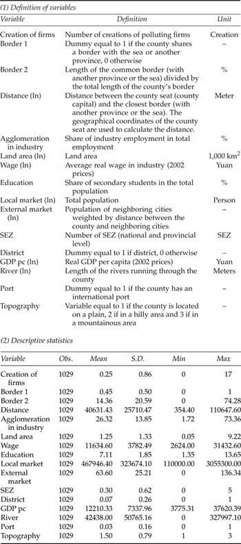
Finally, we introduce a set of indicators for natural endowments. First, we introduce the land area of the county, which is expected to positively affect the number of firm births, as it is a proxy for the number of potential sites (Bartik, Reference Bartik1985). Second, the length of rivers running through each county is also introduced, given that many plants need to be located close to freshwater (Ma, Reference Ma2010). Third, as it may be more difficult for a firm to set up in a mountainous area, we control for the topography of the county. Note that the last two control variables are particularly important given that borders are sometimes established by geographical discontinuities (rivers or mountains), which could bias our estimation of the transboundary effect (Holmes, Reference Holmes1998). Lastly, we introduce a dummy variable for districts to reflect the nature of the administrative unit and year dummies in every specification. All of these data come from the Hebei Statistical Yearbooks (2003–2009); the definition of variables and descriptive statistics are provided in Appendix A.Footnote 14
5. Estimation strategy
The dependent variable of the model is the number of polluting firms created in county i at year t. The special nature of the dependent variable (non-negative integers with a high frequency of zeros) has led us to estimate a count-data model. This model estimates how much a 1 per cent change in an explanatory variable x i affects the probability that a firm sets up in territory i. The probability, Prob(y i), of a territory i to receive y i firms is based on a set of characteristics x i of this territory:
 $$Prob\lpar y_i\rpar =f\lpar x_i\rpar$$
The most common way to model this probability function is to assume that the variable y i follows a Poisson distribution. However, the Poisson model is restrictive because it assumes that the conditional mean is equal to the conditional variance of y i (hypothesis of equi-dispersion). The hypothesis of equi-dispersion is poorly respected with data on firms' location choices, as the conditional variance is often higher than the conditional mean, referred to as ‘overdispersion’. Two phenomena can lead to overdispersion: (i) the presence of unobserved heterogeneity and (ii) an excess of zeros.
When overdispersion arises from unobserved heterogeneity, standard deviations obtained are biased and, therefore, statistical inferences are invalid. In this case, the standard solution consists of assuming that the variable y i follows a negative binomial distribution. It can be easily determined whether the negative binomial model is preferred to the Poisson model, by testing whether the parameter alpha is statistically different from zero (see Cameron and Trivedi, Reference Cameron and Trivedi1998).
When overdispersion arises from an excess of zeros (or ‘zero inflation’), the dependent variable y i takes the value zero more times than assumed by the Poisson distribution, which results in biased estimates. Zero inflation arises when two separate processes lead the dependent variable to take the value zero. In the present study, two processes are likely to explain why some counties did not attract any polluting firms from 2002 to 2008. On the one hand, some counties may not be suitable locations for firms and thus they will never attract any, whatever the period considered. This could be the case for counties lacking a river, in mountainous areas and where there are no market opportunities. On the other hand, some counties may be suitable locations for firms but did not attract any new firms from 2002 to 2008. To distinguish between the two processes generating a zero outcome, Greene (Reference Greene1994) proposes estimating a zero-inflated Poisson (ZIP) model which essentially consists of integrating a probit model into the Poisson regression model. Specifically, a probit equation is first estimated to distinguish those territories that will never attract any firms from the others. In a second step, the standard Poisson model is estimated.
Lastly, overdispersion can arise both from unobserved heterogeneity and from an excess of zeros. The suitable model in this case is the zero-inflated negative binomial (ZINB) model.
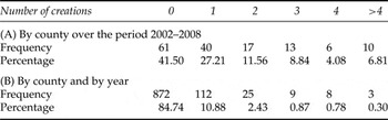
Table 2 gives some insight about the potential zero inflation problem in our sample. The table represents the frequency and percentage of counties with 0, 1, 2, …, creations of firms from 2002 to 2008. According to panel B of the table, when considering the panel dimension of our data, the dependent variable takes the value zero in as much as 84.74 per cent of the cases. The frequency of zeros in our sample is comparable to those in List (Reference List2001) and Roberto (Reference Roberto2004) who estimate a zero-inflated model.
Distribution of firms created

In terms of the testing procedure, as the Poisson (negative binomial) model and the ZIP (ZINB) model are not nested, the Vuong test (Reference Vuong1989) is used to test for zero inflation. Asymptotically, the Vuong test statistic has a standard normal distribution and hence the test statistic obtained must be compared with the critical value of the normal distribution (1.96). A value above 1.96 (below −1.96, respectively) rejects the standard model (zero-inflated model) in favor of the zero-inflated model (standard model).
6. Estimation results
6.1. Testing for the appropriate model
To determine the model that best fits our data, we (i) test the validity of the equi-dispersion hypothesis and (ii) investigate the source(s) of overdispersion.
Appendix A already gives us some insight about the presence of overdispersion in our data. Indeed, the standard deviation of the dependent variable is more than three times its mean. In addition, we estimate the model, assuming that the number of firm births follows a Poisson distribution. The chi-square value obtained is very high, indicating that the Poisson distribution is not suitableFootnote 15 (see Cameron and Trivedi, Reference Cameron and Trivedi1998).
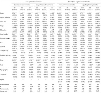
The second step consists of testing whether overdispersion arises from unobserved heterogeneity and/or from an excess of zeros. As shown in table 2, we are very likely to face a problem of zero inflation, which could lead to biased estimates. Thus, we further investigate the presence of zero inflation with the Vuong test. The Vuong statistics are reported at the bottom of table 3. Table 3 gives the estimation results of the ZIP and of the ZINB models.Footnote 16 In each case, six different equations are estimated, depending on the variable of interest introduced (Border1, Border2 and Distance) and on whether or not a time lag is introduced between the dependent and the explanatory variables.Footnote 17 In all 12 cases, the Vuong test clearly rejects the standard model in favor of the zero-inflated model, indicating that zero inflation must be taken into account to obtain consistent estimates.
Baseline results: ZIP and ZINB models

Note: P-values in parenthesis: *p<0.1, **p<0.05,***p<0.01.
In addition, the parameter alpha estimated with the ZINB model provides information on whether overdispersion also arises from unobserved heterogeneity. In five cases out of six, the parameter is not statistically different from zero, indicating that the ZIP better fits our data.Footnote 18 As a consequence, in this paper, we carry out the analysis by estimating a pooled ZIP model, which enables us to take into account overdispersion arising from an excess of zeros.
6.2. Does transboundary pollution exist in China?
According to table 3, the variable of interest has the expected sign and is statistically significant in every case. Counties that share a (larger part of their) border with another province or with the sea have a higher probability of polluting firms locating there. In the same way, the further the county seat is from the boundary, the lower the probability of polluting firms settling there. These results provide evidence of transboundary pollution problems in China. If this has already been demonstrated for the US case, to our knowledge, we are the first to demonstrate this phenomenon in China.
Regarding the control variables, their sign and significance are consistent and robust. The larger the land area, the local market and the GDP per capita, the higher the number of firm births. Conversely, the higher the labor costs, the lower the number of firm births. Moreover, polluting firms set up more frequently in urban districts and in counties where fresh water is available. This confirms that the location choice of Chinese firms nowadays is based on economic factors.
6.3. Robustness checks
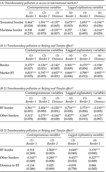
According to the above estimates, we conclude that there is transboundary pollution in Hebei. However, polluting firms could set up in border counties for other factors, and in particular to benefit from better market access. Indeed, Hebei is a unique province in terms of its geography as it (i) shares borders with the Yellow Sea and (ii) surrounds Beijing and Tianjin municipalities (see figure 1). Thus, polluting firms could set up more frequently in border counties in order to benefit from the access to international markets or from the proximity to Beijing and Tianjin markets. The two following subsections further test for transboundary pollution by explicitly controlling for international market access and for the proximity to Beijing and Tianjin.
6.3.1. Transboundary pollution or access to international markets?
To check whether our results are driven by international market access, we separate counties that share a common border with another province from those that share a border with the sea.Footnote 19 ‘Terrestrial border’ refers to counties that border another province while ‘Maritime border’ refers to counties bordering the Yellow Sea.Footnote 20 If polluting firms set up in border counties only to benefit from good access to international markets, the coefficient associated with the variable Terrestrial border should not be significant. The results of the estimations, given in panel A of Table 4,Footnote 21 clearly indicate that the results are not driven by international market access. Indeed, in every estimation, the coefficient associated with the variable Terrestrial border is of expected sign and statistically significant.
Robustness checks: controlling for market access

Notes: These models use the same control variables as the models shown in table 3.
P-values in parenthesis: *p<0.1, **p<0.05,***p<0.01.
6.3.2. Transboundary pollution or access to the Beijing and Tianjin markets?
We investigate the possibility that the higher number of firm births close to borders is due to the proximity to Beijing and Tianjin rather than related to transboundary pollution using three robustness checks.
First of all, we add an additional variable, to control for the proximity to the Beijing and Tianjin markets, to the baseline model estimated in section 6.2. The Beijing and Tianjin market variable is constructed using the measure proposed by Harris (Reference Harris1954):
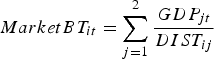 $$Market BT_{it}=\sum_{j=1}^2{GDP_{jt} \over DIST_{ij}}$$
where i refers to the county (county, districts or city at county level) in Hebei and j to the municipalities of Beijing and Tianjin. DIST ij is the number of kilometers from the county seat of i to the county seat of j and GDP jt is the GDP of city j at year t.Footnote 22 Results are reported in panel B-1 of table 4. The coefficient associated with the indicator of proximity to Beijing and Tianjin is positive and significant, attesting that proximity to these municipalities plays a role in attracting polluting firms. Consistently, this leads to a reduction in the size and significance of our coefficients of interest, if we compare these with the baseline estimations reported in table 3. However, it does not alter our main results, given that the coefficient of interest remains significant in every case.
To provide stronger evidence that the results are not driven by proximity to Beijing and Tianjin, we carry out a second robustness check in which we distinguish the Beijing and Tianjin borders from the others. ‘BT border’ refers to counties that border Beijing or Tianjin while ‘Other borders’ refers to counties that share a border other than those with Beijing or Tianjin. Results are reported in panel B-2 of table 4. In every estimation, both the coefficients associated with the BT border and the Other borders variables have the expected sign and are significant, providing strong evidence of transboundary pollution. In addition, in all six cases, the coefficient associated to BT border is higher and generally more significant that those associated to Other borders. This is clearly due to the fact that the variable BT border captures both the effect of transboundary pollution and of market access while Other borders captures only the effect of transboundary pollution.
Finally, some border counties do not directly share a common border with Beijing or Tianjin but are located very close to these municipalities. This is especially the case for counties bordering Inner Mongolia, Liaoning and to some extent Shandong and Shanxi. Thus, the variable Other borders could still capture the Beijing and Tianjin market effect. Consequently, we undertake a third robustness check in which we separate BT border from Other borders and, in addition, in which we control for the distance to Beijing and Tianjin. Results, reported in panel B-3 of table 4, show that the variable Other borders remains significant.
6.4. Has transboundary pollution increased over time?
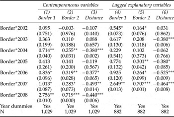
One novel contribution of the present paper is to test whether polluting firms have increasingly set up in border counties over time. To do that, an interactive variable ‘Border*Year’ is introduced into the model. Table 5 gives the estimation results for the coefficients of interest (the full estimation results are available in the supplementary Appendix S.10). According to these estimations, border counties have become increasingly attractive destinations over the period studied. Indeed, while during the first years of the sample the variable of interest is not significant or not robust, it becomes significant and its coefficient increases each year. Several elements can explain the increasing attractiveness of border counties. Firstly, because of the Beijing Olympics in 2008, some polluting firms located in Beijing were closed and re-opened in the neighboring province of Hebei. The Olympic Games also made the creation of polluting firms in Beijing more difficult. It is possible that firms wishing to set up in Beijing moved to Hebei, as no better option was available, and set up as close as possible to Beijing, i.e., in the counties sharing a border with Beijing. Secondly, as discussed in section 4.1, environmental policy in China has been tightened since 2000, which may have led to a perverse effect: as firms are increasingly sensitive to environmental regulations, they are more attracted to the border counties over time. Finally, the increasing number of citizen complaints regarding pollution, as well as the change in the political promotion system, could have led local regulators to intensify the implementation of the environmental policy, particularly in interior counties.
Has transboundary pollution increased over time?

Notes: These models use the same control variables as the models shown in Table 3.
P-values in parenthesis: *p<0.1, **p<0.05,***p<0.01.
7. Conclusion
This paper proposes a comprehensive study of transboundary pollution problems in China. To do so, we estimate whether polluting firms are more likely to set up in counties close to the regional border. Our estimation results suggest that the closer a county is to the provincial border, the higher the probability of it attracting polluting firms. Thus, there is a risk that people in border counties suffer disproportionately from pollution. Transboundary pollution appears to be a particularly significant problem in China as we have found that the effect has increased over time.
If transboundary pollution problems are often put forward by opponents of decentralization, our results do not suggest that a centralized policy would be optimal. Indeed, a decentralized policy offers compelling advantages for a country as heterogeneous as China. While a centralized policy would consist of applying uniform rules across the country, a decentralized policy allows for adaption to the local conditions and thus is more efficient. Lipscomb and Mobarak (Reference Lipscomb and Mobarak2007) also estimate that decentralization leads to an increase in local government budgets. According to the authors, in Brazil pollution spillovers and budget increases arising from decentralization compensate each other so that, in the end, the estimated net effect of decentralization on water quality is zero. It is unclear whether a decentralized or a centralized policy would lead to higher social welfare in our case. Thus, as suggested by Sigman (Reference Sigman2005) in the case of the United States, the optimal policy might be to provide targeted solutions to transboundary pollution problems within the framework of a decentralized policy. The recent creation of the six major regional centers (see section 2.1.) could be a way to reduce transboundary pollution. For the moment, the creation of these centers is too recent and their power is still too limited to have measurable impact. It could be interesting to study the location choices of firms in the period to come, to test whether the creation of these intermediate poles, between central government and regional governments, may offer a solution to the transboundary pollution problem. In addition, some provinces have recently released data on pollution emissions for each facility on the list published by the MEP and the provincial EPB. Thus, Schoolman and Ma (Reference Schoolman and Ma2011) combine data on sources of pollution and pollution emissions data on every source for Jiangsu province. It would be interesting to further test for transboundary pollution by using this actual pollution data rather than the counting of firms. This would enable us to investigate more precisely whether populations at borders are disproportionately exposed to pollution.
Supplementary material and methods
The Supplementary material referred to in this paper can be found online at journals.cambridge.org/EDE.
Variables definitions and descriptive statistics