1. Introduction
In the paper, we investigate a steady two-dimensional free-surface flow past a point vortex. The fluid is assumed to be ideal and incompressible, and the depth of the fluid is infinite. The flow moves from left to right with uniform speed
 $c$
far upstream and is subject to the downward acceleration
 $g$
of gravity. The capillary forces are neglected. A point vortex of circulation
 $\varGamma$
is located at depth
 $H$
. The positive direction of circulation is counterclockwise. Everywhere except the point of the vortex location, the flow is supposed to be irrotational. Such a flow is characterised by two dimensionless parameters, those being the dimensionless vortex circulation
 $\gamma =\varGamma /(\textit{cH}\,)$
and the Froude number
 $ \textit{Fr}=c/\sqrt {gH}$
(see figure 1
a).
A characteristic feature of the free-surface flow past a disturbance (a body or a point singularity) is the formation of an infinite downstream wave train. This means that if
 $y=y_s(x)$
is the equation of the free surface, then as
 $x\to \pm \infty$
, we have
 \begin{align} \lim _{x\to -\infty }y_s(x)=0,\quad \lim _{n\to \infty }y_s(x+n\lambda )=y_s^*(x), \end{align}
where
 $n\in \mathbb{N}$
,
 $\lambda$
is an unknown in advance wavelength at infinity and
 $y_s^*(x)$
is a
 $\lambda$
-periodic function that defines the free surface of Stokes’ wave far downstream.
In the traditional linear formulation, solutions for point sources, vortices and dipoles in fluids of finite and infinite depth are reviewed by Wehausen & Laitone (Reference Wehausen and Laitone1960), and the case of infinite depth is considered in detail by Kochin, Kibel’ & Roze (Reference Kochin, Kibel’ and Roze1964). In the nonlinear formulation, the flow past a point vortex was studied in several works. The case of finite depth was investigated by Salvesen & von Kerczek (Reference Salvesen and von Kerczek1976), Maklakov (Reference Maklakov1995) (subcritical flow) and by Doak & Vanden-Broeck (Reference Doak and Vanden-Broeck2017) (supercritical flow). The case of infinite depth was studied by Forbes (Reference Forbes1985), Liao (Reference Liao1992) and Shelton & Trinh (Reference Shelton and Trinh2023).
The goal of the paper is to find the solutions of the solitary wave type, when
 $y_s^*(x)\equiv 0$
for any
 $\lambda \gt 0$
(see figure 1
b). These solutions are waveless far downstream and, in addition, have a vertical line of symmetry. In the works of Hur (Reference Hur2012) and Ifrim & Tataru (Reference Ifrim and Tataru2020), it was mathematically rigorously proven that in flow of infinite depth without disturbances, there are no pure gravity solitary waves. The situation changes if in the flow, there is a point vortex. In the paper, we present numerical evidence that for a fixed Froude number
 $ \textit{Fr}\le 0.8$
, there exists a finite set of positive
 $\gamma$
for which the solutions of the solitary wave type occur. Moreover, these solutions can have several crests on the free surface. Accurate numerical computations show that at
 $ \textit{Fr}=0.8$
, we have only one such solution with one crest on the free surface; at
 $ \textit{Fr}=0.7$
, the number of waveless solutions is already four and they have from one to four crests; and at
 $ \textit{Fr}=0.6$
, this number increases up to eleven with the number of crests that varies from one to eleven.
(a) Flow with an infinite wave train. (b) Flow of the solitary wave type. (c) Auxiliary flow past two vortices. (d) Parametric
 $t$
-plane.

2. Formulations of the main and auxiliary problems
Consider the flow shown in figure 1(a). The Cartesian coordinate system
 $Oxy$
is chosen so that the
 $y$
-axis is directed opposite to the gravity acceleration
 $g$
, and the vortex is located at the point
 $(0,-H)$
. Let us introduce the complex coordinate
 $z=x+{\mathrm{i}} y$
(
 ${\mathrm{i}}=\sqrt {-1}$
), the complex potential
 $w= \varphi (x,y)+{\mathrm{i}} \psi (x,y)$
and the complex conjugate velocity
 $f(z)=w'(z)=v_x(x,y)-{\mathrm{i}} v_y(x,y)$
, where
 $v_x$
and
 $v_y$
are the components of the velocity vector. For the flow shown in figure 1(a), the domain of definition
 $D_z$
of the function
 $f(z)$
is determined as follows:
 \begin{equation} D_z=\{z=x+{\mathrm{i}} y \in D_z \Leftrightarrow y\le y_s(x)\}. \end{equation}
Now, we formulate the boundary-value problem for finding the analytic function
 $f(z)$
and the unknown free surface
 $y=y_s(x)$
. In the vicinity of the point
 $z=-{\mathrm{i}} H$
, we have
 \begin{equation} f(z)=\frac {\varGamma }{2\pi {\mathrm{i}}}\frac {1}{z+{\mathrm{i}} H}+a_0+O(z+{\mathrm{i}} H), \end{equation}
where
 $a_0 \neq 0$
is a complex number. We should note that the solutions of the solitary wave type are only possible if
 $a_0 \neq 0$
. This means that the point vortex is not carried with the wave, but rather acts as forcing. A non-existence theorem of solitary waves in fluid of infinite depth for the case
 $a_0 = 0$
under some natural restrictions on the free surface shape was proven by Chen, Walsh & Wheeler (Reference Chen, Walsh and Wheeler2019).
The free surface
 $y=y_s(x)$
is a streamline, and hence the kinematic boundary condition on it is
 \begin{equation} {\mathop {\textrm {Im}}\nolimits } f[x+{\mathrm{i}} y_s(x)]+ y_s'(x){\mathop {\textrm {Re}}\nolimits } f[x+{\mathrm{i}} y_s(x)]=0, \quad x\in \mathbb{R}. \end{equation}
The dynamic boundary condition follows from the Bernoulli equation:
 \begin{equation} \left |f\left [x+{\mathrm{i}} y_s(x)\right ]\right |^2+ 2 g y_s(x)=c^2, \quad x\in \mathbb{R}. \end{equation}
The conditions at infinity for
 $f(z)$
are
 \begin{align} \lim _{x\to -\infty } f(x+{\mathrm{i}} y)=c, \quad \lim _{y\to -\infty } f(x+{\mathrm{i}} y)=c, \quad \lim _{x\to +\infty } f(x+{\mathrm{i}} y)\lt \infty . \end{align}
To these conditions at infinity, we should add condition (1.1) for the function
 $y=y_s(x)$
.
The main difficulty in solving numerically the boundary value problem (1.1), (2.2)–(2.5) is an infinite wave train. The matter is that at present time, there are no strict mathematical estimates of the difference
 $y_s(x) - y_s^*(x)$
. Approximate methods for modelling the wave train are described in the monograph by Vanden-Broeck (Reference Vanden-Broeck2010). These methods are based on cutting off the infinite computational domain on the left and right, thereby turning this domain into a finite one. At the same time, there is no strict mathematical formulation of the boundary-value problem obtained as a result of this cutoff.
To get such a formulation, we proceed as follows. On the free surface
 $y=y_s(x)$
, we take a point
 $B$
lying on a crest or trough with abscissa
 $x=x_B$
. This means that
 $y_s'(x_B)=0$
. From the point
 $B$
, we draw an equipotential
 $\textit{BA}^{\prime}$
, where
 $A'$
is the infinitely distant point of the flow in the downward
 $y$
-direction (see figure 1
a). If the point
 $B$
is at a sufficient distance from the vortex, then this equipotential will be close to the vertical straight line
 $x=x_B$
. We replace it with the straight line
 $x=x_B$
. Since the line
 $x=x_B$
is an equipotential, the boundary condition on it is
 \begin{equation} {\mathop {\textrm {Im}}\nolimits } f(z)=0, \quad z =x_B+{\mathrm{i}} y. \end{equation}
Consider the domain
 \begin{equation} D_z'=\big\{z=x+{\mathrm{i}} y\in D_z' \Leftrightarrow y \le y_s(x)\bigcap x\le x_B\big\}. \end{equation}
The function
 $f(z)$
in this domain will satisfy the boundary conditions (2.2)–(2.4), (2.6); however, instead of (1.1), (2.5), we will have simpler conditions
 \begin{align} \lim _{z\to \infty } f(z)=c, \quad \lim _{x\to -\infty }y_s(x)=0. \end{align}
Due to the boundary condition (2.6) and the Riemann–Schwarz symmetry principle, the function
 $f(z)$
can be analytically continued from the region
 $D_z'$
through the line
 $\textit{BA}^{\prime}$
to the region that is the mirror image of the region
 $D_z'$
with respect to the line
 $\textit{BA}^{\prime}$
. As a result, we obtain the flow shown in figure 1(c) with two vortices of equal circulations located at the distance
 $2 x_B$
from each other.
We call the main problem the problem of determining
 $f(z)$
in the domain
 $D_z$
and we call the auxiliary problem that in the domain
 $D_z'$
. Thus, the auxiliary problem is obtained from the main problem by choosing the point
 $x_B$
. Since for the main problem the equation
 $y_s'(x)=0$
has a countable set of solutions, the auxiliary problem will also have a countable set of solutions. This means that in addition to two dimensionless parameters of the main problem
 $\gamma$
and
 $ \textit{Fr}$
, the solution of the auxiliary problem will depend on some integer parameter
 $m\ge 0$
that determines one of the roots of the equation
 $y_s'(x)=0$
.
Note that the flow shown in figure 1(c) was recently studied by Shelton & Trinh (Reference Shelton and Trinh2023). This flow is waveless both upstream and downstream with waves arising between two vortices. The main goal of this paper is to find a waveless solution to the main problem (see figure 1
b). For this purpose, we will use the solution of the auxiliary problem. If
 $x_B\gg 1$
, then the auxiliary problem approximately models an infinite wave train, which makes it possible, for fixed Froude numbers
 $ \textit{Fr}$
, to determine numerically approximate values of
 $\gamma$
for which the waves between vortices will be absent. If
 $x_B=0$
, then two vortices with circulations
 $\gamma$
will merge into one with double circulation
 $2\gamma$
and we will obtain an accurate waveless numerical solution to the main problem.
3. Auxiliary problem in the parametric
 $\boldsymbol{t}$
-plane

Let us map conformally the flow region
 $D_z'$
onto the upper semicircle
 $D_t$
of the parametric plane
 $t=\xi +{\mathrm{i}} \eta$
. The correspondence of points between the physical
 $z$
-plane and the parametric
 $t$
-plane is as follows:
 $A,A'\sim -1$
,
 $B\sim 1$
,
 ${\mathrm{i}} H \sim {\mathrm{i}}\rho$
, where
 $\rho \in (0,1)$
is an unknown parameter. The domain
 $D_t$
is shown in figure 1(d).
We shall seek for the derivative of the conformal mapping from
 $D_t$
onto
 $D_z'$
in the form
 \begin{equation} z'(t)=k\left [\frac {{\mathrm{i}}}{(t+1)^2}+\frac {\omega (t)}{{\mathrm{i}} t}\right ]\!, \end{equation}
where
 $\omega (t)$
is an unknown analytic function in the domain
 $D_t$
and
 $k\gt 0$
is an unknown parameter, which has the dimension of length.
By virtue of analyticity of
 $z'(t)$
at the point
 $t=0$
and the boundary condition
 ${\mathop {\textrm {Re}}\nolimits } z'(\xi )=0$
for
 $\xi \in [-1,1]$
, the function
 $\omega (t)$
satisfies the following boundary conditions:
 \begin{align} \omega (0)=0;\quad {\mathop {\textrm {Im}}\nolimits }\,\omega (\xi )=0,\;\; \xi \in [-1,1]. \end{align}
Now, we express the parameter
 $k$
in terms of
 $\rho$
and
 $\omega (t)$
. To do so, we first find by integration the complex coordinate
 $z_B$
of the point
 $B$
:
 \begin{align} z_B=-{\mathrm{i}} H+k\left [\frac {\rho }{1+\rho ^2} + \frac {{\mathrm{i}}}{2}\frac {1-\rho ^2}{1+\rho ^2}+{\mathrm{i}} J({\mathrm{i}} \rho )\right]\!, \quad J(t)=\int _1^t\frac {\omega (t_1)\,{\mathrm{d}} t_1}{t_1}. \end{align}
Then, the conformal mapping of the domain
 $D_t$
onto
 $D_z'$
is
 \begin{equation} z(t)=z_B+k{\mathrm{i}} \left [\frac {1}{2}\,\frac {t-1}{t+1}-J(t)\right ]\!. \end{equation}
We denote
 $\omega ({\mathrm{e}}^{{{i}}\sigma })=\mu (\sigma )+{\mathrm{i}} \tau (\sigma )$
, where
 $\sigma$
is the polar angle in the
 $t$
-plane. The shape of the free surface
 $y=y_s(x)$
can be found from the parametric equations
 \begin{align} x(\sigma ) & = x_B+k\left [-\frac {1}{2}\tan \frac {\sigma }{2}+\int _0^\sigma \mu (\sigma _1)\,{\mathrm{d}} \sigma _1\right ]\!, \nonumber \\ y(\sigma )& = y_B+k\int _0^\sigma \tau (\sigma _1)\,{\mathrm{d}} \sigma _1, \quad \sigma \in [0,\pi ], \\[-28pt] \nonumber \end{align}
 \begin{align} x_B=k\left [\frac {\rho }{1+\rho ^2}-{\mathop {\textrm {Im}}\nolimits } J({\mathrm{i}} \rho )\right ]\!, \quad y_B=-H+k\left [\frac {1}{2}\frac {1-\rho ^2}{1+\rho ^2}+{\mathop {\textrm {Re}}\nolimits } J({\mathrm{i}} \rho )\right ]\!. \\[2pt] \nonumber \end{align}
According to (2.8b
), we have
 $y_s(-\infty )=0$
; therefore,
 $y(\pi )=0$
. Hence, from (3.5b
) and (3.6b
), we deduce that
 \begin{align} k=\frac {H}{I}, \quad I=\frac {1}{2}\frac {1-\rho ^2}{1+\rho ^2}+{\mathop {\textrm {Re}}\nolimits } J({\mathrm{i}} \rho )+\int _0^\pi \tau (\sigma )\,{\mathrm{d}}\sigma . \end{align}
Now, we determine the complex potential
 $w$
and its derivative
 $w'(t)$
as functions of
 $t$
. Using Chaplygin’s singular point method (see Gurevich Reference Gurevich1966 for details), we find
 \begin{align} w(t) = \frac {\varGamma }{2 \pi {\mathrm{i}}} \log \frac {t^2 + \rho ^2}{1 + \rho ^2 t^2} - \frac {k c {\mathrm{i}}}{t + 1}, \quad w'(t)= k c {\mathrm{i}} \left [\frac {1}{(t+1)^2}-\frac {\gamma _0 (1-\rho ^4)t}{(t^2+\rho ^2)(1+\rho ^2 t^2)}\right ]\!, \end{align}
where
 $\gamma _0=\varGamma /(\pi k c)$
. The complex conjugate velocity
 $f$
as a function of
 $t$
is given by the equation
 $f(t)=w'(t)/z'(t)$
. This equation together with (3.4) determine the function
 $f(z)$
in the parametric form. If
 $k=H/I$
, the function
 $f(z)$
defined in such a manner satisfies the boundary conditions (2.2), (2.3) and (2.8). The remainder condition is (2.4), which, after a little algebra, can be rewritten in the form
 \begin{equation} 4 \frac {f_1(\sigma )+F(\mu ,\tau ,\sigma )}{1-8 F(\mu ,\tau ,\sigma )\cos ^2(\sigma /2)}+E \theta (\sigma )=0, \end{equation}
where
 $E=gk/c^2$
,
 $F(\mu ,\tau ,\sigma )=\mu (\sigma )-2 \cos ^2(\sigma /2) [\mu ^2(\sigma )+\tau ^2(\sigma ) ]$
,
 \begin{align} \theta (\sigma )=\frac {1}{\cos ^2(\sigma /2)}\int _\pi ^\sigma \tau (\sigma _1)\,{\mathrm{d}} \sigma _1, \\[-28pt] \nonumber \end{align}
 \begin{align} f_1(\sigma )=\gamma _0 f_0(\sigma )\left [2 \gamma _0 f_0(\sigma )\cos ^2\frac {\sigma }{2}-1\right ]\!, \quad f_0(\sigma )=\frac {1-\rho ^4}{\rho ^4+2 \rho ^2\cos 2\sigma +1}. \\[2pt] \nonumber \end{align}
The boundary condition (3.9) contains three unknown parameters:
 $\rho$
,
 $\gamma _0$
and
 $E$
. To determine these parameters, it needs to have three conditions. One of them is condition (3.2a
). Two more conditions follow from the equations
 \begin{align} k=\frac {H}{I},\quad \gamma _0=\frac {\varGamma }{\pi k c}=\frac {\gamma I}{\pi },\quad E=\frac {g k}{c^2}=\frac {1}{\textit{Fr}^2 I}. \end{align}
Taking into account that
 $\gamma =\varGamma /(\textit{cH}\,)$
and
 $ \textit{Fr}=c/\sqrt {g H}$
are given, we get
 \begin{align} I-\frac {\pi }{\gamma }\gamma _0=0,\quad \frac {\pi }{\gamma }E\gamma _0-\frac {1}{\textit{Fr}^2}=0, \end{align}
where
 $I$
is determined from (3.7b
).
At the given
 $\gamma$
and
 $ \textit{Fr}$
, the boundary conditions (3.2b
), (3.9) and the complementary relations (3.2a
), (3.13) allow us to find the analytic function
 $\omega (t)$
and the parameters
 $\rho$
,
 $\gamma _0$
and
 $E$
. In certain cases, we shall solve the problem (3.2), (3.9) and (3.13) in the following formulation: the parameters
 $ \textit{Fr}$
and
 $\rho$
are given, whereas
 $\gamma$
,
 $\gamma _0$
and
 $E$
are unknown.
4. Discretisation and an initial approximation for application of Newton’s method
In what follows, we assume that
 $H=1$
, so
 $H$
is the reference length. We put the mesh of
 $N$
knots
 $\sigma _i=(i-1)\pi /(N-1)$
,
 $i=\overline {1,N}$
on the segment
 $[0,\pi ]$
. We shall seek for the function
 $\omega (t)$
in the form of a truncated power series:
 \begin{equation} \omega (t)=\sum _{n=1}^N c_n t^{n-1}, \end{equation}
where
 $c_n$
are real coefficients. Then, the condition (3.2b
) is fulfilled. We introduce the following notation:
 $\mu _i=\mu (\sigma _i$
),
 $\tau _i=\tau (\sigma _i)$
,
 $\theta _i=\theta (\sigma _i)$
. According to (3.10) and (4.1),
 \begin{align} \mu _i=c_1+\sum _{n=2}^{N-1}c_n\cos (n-1)\sigma _i+(-1)^{i-1}c_N,\quad \tau _i=\sum _{n=2}^{N-1}c_n\sin (n-1)\sigma _i, \\[-28pt] \nonumber \end{align}
 \begin{align} \theta _i=\left \{ \begin{array}{ll} \displaystyle -\frac {1}{\cos ^2(\sigma _i/2)}\sum _{n=2}^N\frac {c_n}{n-1}\big [\cos (n-1)\sigma _i-(-1)^{n-1}\big ],& i=\overline {1,N-1},\\[0.5em] \displaystyle -2\sum _{n=2}^N(n-1)(-1)^n c_n,& i=N. \end{array}\right . \\[2pt] \nonumber \end{align}
In (4.2), we have taken into account that
 $(N-1)\sigma _i=(i-1)\pi$
. The value
 $\theta _N$
in (4.3) has been calculated with the help of L’Hopital’s rule. The technique of fast Fourier transform makes it possible to compute the coefficients of the square matrices
 $C_{\textit{ij}}$
,
 $D_{\textit{ij}}$
and
 $\varTheta _{\textit{ij}}$
such that
 \begin{align} c_i=\sum _{j=1}^N C_{\textit{ij}}\mu_{\kern-1pt j}, \quad \tau _i=\sum _{j=1}^N D_{\textit{ij}}\mu_{\kern-1pt j}, \quad \theta _i=\sum _{j=1}^N \varTheta _{\textit{ij}}\mu_{\kern-1pt j}. \end{align}
Now, from the boundary condition (3.9), we obtain the system of
 $N$
nonlinear equations
 \begin{equation} 4 \frac {f_1(\sigma _i)+F_i}{1-8 F_i\cos ^2(\sigma _i/2)}+E\sum _{j=1}^N \varTheta _{\textit{ij}}\mu_{\kern-1pt j} =0, \quad i=\overline {1,N}, \end{equation}
where
 \begin{equation} F_i=\mu _i-2 \cos ^2\frac {\sigma _i}{2}\left [\mu _i^2+\left (\sum _{j=1}^N D_{\textit{ij}}\mu_{\kern-1pt j}\right )^2\right ]\!. \end{equation}
We should add the following equation to system (4.5):
 \begin{align} \sum _{j=1}^N \alpha _j \mu_{\kern-1pt j}=0, \quad \alpha _j=\left \{\begin{array}{ll} 1/2,& j=1 \bigcup j=N,\\[0.2em] 1,& j=\overline {2,N-1}, \end{array}\right . \end{align}
which is the discrete analogue of the condition
 $\omega (0)=0$
, and the relations (3.13), where in (3.13a
), according to (3.3b
), (3.7b
), (4.1) and (4.4c
),
 \begin{align} I& =\frac {1}{2}\frac {1-\rho ^2}{1+\rho ^2}+{\mathop {\textrm {Re}}\nolimits } J({\mathrm{i}} \rho )-\sum _{j=1}^N\varTheta _{1j}\mu_{\kern-1pt j},\quad J(t)=\sum _{j=1}^N\beta _j(t)\mu_{\kern-1pt j}, \nonumber \\ \beta _j(t)&=\sum _{n=2}^N C_{nj}\frac {t^{n-1}-1}{n-1}. \end{align}
Thus, we have obtained the system (4.5), (4.7a
), (3.13) of
 $N+3$
equations. At the given
 $\gamma$
and
 $ \textit{Fr}$
, the
 $N+3$
unknowns in the system are
 $\mu_{\kern-1pt j}$
,
 $\rho$
,
 $\gamma _0$
and
 $E$
. At the given
 $\rho$
and
 $ \textit{Fr}$
, the
 $N+3$
unknowns are
 $\mu_{\kern-1pt j}$
,
 $\gamma _0$
,
 $\gamma$
and
 $E$
. For both cases, the system has been solved by Newton’s method. The iteration process is repeated until the maximum residual error is less than
 $10^{-14}$
. To achieve this accuracy, 5–6 iterations of Newton’s method are usually required.
The formulation of the auxiliary problem contains an integer parameter
 $m$
, which determines the root of the equation
 $y_s'(x_B)=0$
. This parameter is not explicitly included in the system (4.5), (4.7a
), (3.13). However, it appears when solving the linear problem, whose solution, for small
 $\gamma$
, serves as an initial approximation for the iterations of Newton’s method. Assume that
 $\gamma$
is a small parameter, and the functions
 $\mu (\sigma )$
and
 $\tau (\sigma )$
are of order
 $\gamma$
. Retaining only first-order terms in the boundary condition (3.9) yields
 \begin{equation} 4\mu (\sigma )+E \theta (\sigma )=4\gamma _0 f_0(\sigma ). \end{equation}
According to (3.7b ) and (3.12),
 \begin{align} I=\frac {1}{2}\frac {1-\rho ^2}{1+\rho ^2}, \quad \gamma _0=\frac {\gamma }{2\pi }\frac {1-\rho ^2}{1+\rho ^2}, \quad E=\frac {2}{\textit{Fr}^2}\frac {1+\rho ^2}{1-\rho ^2}. \end{align}
So, in (4.9), the parameters
 $\gamma _0$
and
 $E$
are defined by (4.10b
,
c
). In addition to (4.9), the function
 $\omega (t)$
must satisfy conditions (3.2).
It is to be noted that in (4.9) and (4.10), the parameter
 $\rho$
is unknown. To find
 $\rho$
, we proceed as follows. If we have two vortices located at the points
 $(0,-1)$
and
 $(2 x_B,-1)$
, then according to Kochin et al. (Reference Kochin, Kibel’ and Roze1964), Forbes (Reference Forbes1985) and the linearity of the problem, the function
 $y_s^*(x)$
, defined in (1.1b
), is given by the formula
 \begin{align} y_s^*(x)& =2 \gamma {\mathrm{e}}^{-1/\textit{Fr}^2}\left [ \sin \left (\frac {x}{\textit{Fr}^2}\right )+\sin \left (\frac {x-2 x_B}{\textit{Fr}^2}\right )\right ] \nonumber \\ & = 4 \gamma {\mathrm{e}}^{-1/\textit{Fr}^2}\sin \left (\frac {x-x_B}{\textit{Fr}^2}\right )\cos \left (\frac {x_B}{\textit{Fr}^2}\right )\!. \end{align}
Since the flow shown in figure 1(c) is waveless,
 $y_s^*(x)\equiv 0$
in (4.11). Therefore,
 \begin{align} \cos \left (\frac {x_B}{\textit{Fr}^2}\right )=0\;\; \Rightarrow \;\; x_B= \textit{Fr}^2 \frac {\pi }{2}(2m+1), \end{align}
where
 $m$
is a non-negative integer number. As follows from (3.6a
), (3.12a
) and (4.10a
),
 \begin{align} k=\frac {2(1+\rho ^2)}{1-\rho ^2},\quad x_B=k\frac {\rho }{1+\rho ^2}=\frac {2 \rho }{1-\rho ^2}\; \Rightarrow \; \rho =\frac {1}{x_B}\left (\sqrt {x_B^2+1}-1\right )\!, \end{align}
where the last formula is derived by solving the square equation
 $x_B\rho ^2+2\rho -x_B=0$
with respect to
 $\rho$
. Thus, in the boundary condition (4.9), the parameters
 $\rho$
,
 $\gamma _0$
and
 $E$
are known. The discrete analogue of (4.9) is
 \begin{equation} 4\mu _i+E\sum _{j=1}^N\varTheta _{\textit{ij}}\mu_{\kern-1pt j}=4\gamma _0 f_0(\sigma _i), \quad i=\overline {1,N}. \end{equation}
The system (4.14) is a linear system of
 $N$
equations with
 $N$
unknowns. However, the matrix of this system turns out to be ill-conditioned. For this reason, we add (4.7a
) to the system (4.14), which is the discrete analogue of the condition (3.2a
), and solve the overdetermined system of
 $N+1$
equations with
 $N$
unknowns by the least square technique. Using such an approach, we find the initial values of
 $\mu _i$
, (
 $i=\overline {1,N}$
),
 $\rho$
,
 $\gamma _0$
and
 $E$
that provide the convergence of Newton’s iterations for the system (4.5), (4.7a
), (3.13) at small
 $|\gamma |$
.
5. Solutions of the solitary wave type
Computations of the free-surface flow past a single vortex, carried out in the works by Forbes (Reference Forbes1985) and Liao (Reference Liao1992), showed that at fixed Froude numbers
 $ \textit{Fr}$
, with decrease of
 $\gamma \lt 0$
, the amplitudes of waves behind the vortex increase monotonically. Therefore, the solutions of the solitary wave type can only occur if
 $\gamma \gt 0$
. To get such solutions, we investigate the auxiliary problem of two vortices. Generally speaking, the waves arising between two vortices are not symmetric with respect to vertical lines drawn from crests or troughs in the downward direction. The only exception is the wave whose crest or trough lie on the line
 $\textit{BA}^{\prime}$
. In figure 1(c), this wave is plotted by a dashed line. We shall call it the median wave. We define the doubled amplitude of the median wave by the formula
 $2 A=y(0)-y(\sigma _*)$
, where
 $\sigma _*$
is the first non-zero root of the equation
 $\tau (\sigma )=0$
.
In figure 2(a), we demonstrate the dependencies
 $2 A$
versus
 $\gamma \gt 0$
at
 $ \textit{Fr}=0.7$
and
 $m=11,21,31$
. The computations have been carried out at
 $N=3{\times }2^{11}+1=6145$
. So, in figure 2(a), three graphs are shown, and in the scales of the figure, all three graphs coincide in the range of
 $\gamma$
where they have been plotted. As one can see, the equation
 $A(\gamma )=0$
has four roots. The values of these roots are presented in table 1. The dashes in the table mean that the corresponding root at the specified
 $m$
has not been obtained. The fourth root has been found only at
 $m=11$
. The change of sign of
 $2 A$
in figure 2(a) means that the crest at the point
 $B$
turns to the trough and vice versa.
(a) Dependencies
 $2 A$
versus
 $\gamma \gt 0$
at
 $ \textit{Fr}=0.7$
and m = 11 (black line), 21 (orange line) and 31 (green line). (b) Four solutions of the solitary wave type at
 $ \textit{Fr}=0.7$
. The value
 $y_{\textit{max}}=\textit{Fr}^2/2$
, labelled by a horizontal line in figure 2(b), is the maximum possible height of the free surface according to the Bernoulli equation.

The most interesting fact is that if
 $A=0$
, then at the corresponding value of
 $\gamma$
, the waves between two vortices disappear and the free surface represents two bumps above each vortex. The shapes of the bumps are almost symmetric with respect to the vertical lines going through the points of vortex location and at
 $m=11$
, are shown in figure 2(b). As one can see, they have from one to four crests on their surfaces depending on the number of the non-zero root of the equation
 $A(\gamma )=0$
. The values of
 $\gamma$
in table 1 at
 $m=11,21,31$
are also very close to each other.
A thorough numerical analysis shows that the found waveless solutions have a very small asymmetry due to the mutual influence of vortices. So, these solutions describe those of the solitary wave type only approximately. To get pure symmetric solutions, we have developed a special algorithm illustrated by figure 3. The idea is to solve the auxiliary problem at small values of
 $m$
trying to get the solution with the parameter
 $\rho =0$
. If
 $\rho =0$
, then according to (3.6a
), the value
 $x_B=0$
(since
 ${\mathop {\textrm {Im}}\nolimits } J(0)=0$
), and two vortices with circulations
 $\gamma$
will merge into one with double circulation
 $2\gamma$
and we will obtain an accurate waveless numerical solution for a single vortex.
The values of
 $\gamma$
at
 $ \textit{Fr}=0.7$
when the amplitude of the median wave is zero. The values for
 $2\gamma _n$
are the accurate values of
 $\gamma$
for solutions of the solitary wave type.

Illustrations to the algorithm of finding four solutions of the solitary wave type at
 $ \textit{Fr}=0.7$
. Four graphs demonstrate continuous branches of solutions that start at small values of
 $\gamma$
and end at
 $x_B=0$
(
 $\rho =0$
), while maintaining a small number of crests and troughs on the free surface. The total number of crests on the whole free surface is
 $m+1$
.

In figure 3, we demonstrate the dependence of the parameter
 $\rho$
on
 $\gamma$
at
 $ \textit{Fr}=0.7$
and
 $m=0,1,2,3$
. First, we secantly increase
 $\gamma$
up to the moment when
 $\rho (\gamma )$
starts to change abruptly (black points in figure 3), after that, we switch the algorithm and secantly decrease
 $\rho$
down to zero value (orange points in figure 3). We denote by
 $\gamma _n$
the value of
 $\gamma$
at which
 $\rho =0$
. Then,
 $2 \gamma _n$
is an accurate value of
 $\gamma$
for which there exists a solution of the solitary wave type. These values are presented in the last line of table 1. One can see a good agreement with approximate
 $\gamma$
found from the equation
 $A(\gamma )=0$
. The waveless free-surface shapes are also demonstrated in figure 2(b) and in the scales of the figure, there is a full coincidence with those plotted at
 $m=11$
.
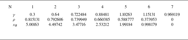
The values of
 $\rho$
,
 $\gamma$
and
 $x_B$
for the curves enumerated in figure 4 (
 $ \textit{Fr}=0.7$
,
 $m=3$
).

Deformations of the left halves of free surfaces at
 $ \textit{Fr}=0.7$
and
 $m=3$
as
 $x_B\to 0$
. The numeration of curves corresponds to the enumerated points in figure 3 (
 $m=3$
).

In figure 4, we demonstrate the deformations of the left halves of free surfaces at
 $ \textit{Fr}=0.7$
and
 $m=3$
as
 $x_B\to 0$
. The numeration of curves corresponds to the enumerated points in figure 3 (
 $m=3$
). As one can see, curve 1 (
 $x_B \approx 5.002$
) has two crests and two troughs. With decrease of
 $x_B$
, the amplitude of wave oscillations decreases (curve 2) and these oscillations fully disappear on curve 3. The incipience of the second crest can be seen on curve 4. With further decrease of
 $x_B$
, the construction ‘two crests–two troughs’ is conserved and at
 $x_B=0$
, we have the left half of the highest curve in figure 2(b). The values of
 $\gamma$
,
 $\rho$
and
 $x_B$
corresponding to the seven curves of figure 4 are presented in table 2.
In a similar manner, we have carried out the computations at
 $ \textit{Fr}=0.6$
and have found 11 waveless solutions with the number of crests on the free surface that varies from one to eleven. The results are shown in table 3 and in figure 5. At
 $ \textit{Fr}=0.8$
, there exists the only one solution of the solitary wave type at
 $\gamma =2 \gamma _n= 0.818824$
.
The values of
 $\gamma$
at
 $ \textit{Fr}=0.6$
when the amplitude of the median wave is zero. The values for
 $2\gamma _n$
are the accurate values of
 $\gamma$
for solutions of the solitary wave type.

Eleven solutions of the solitary wave type at
 $ \textit{Fr}=0.6$
.

6. Comparison with Shelton & Trinh (Reference Shelton and Trinh2023)
In the present paper, we introduce the dimensionless circulation by the formula
 $\gamma =\varGamma /(\textit{cH}\,)$
, where the positive direction of circulation is counterclockwise. Forbes (Reference Forbes1985) denoted the same dimensionless parameter as
 $\varepsilon$
, but since his positive direction of circulation is clockwise, we must set
 $\gamma =-\varepsilon$
. In the work by Shelton & Trinh (Reference Shelton and Trinh2023), the same parameter was denoted as
 $\varGamma _c$
, and according to their figure 1 and their (1.1), the positive direction of circulation is also counterclockwise, so
 $\gamma =\varGamma _c$
.
It seems Forbes (Reference Forbes1985) was the first to notice that the behaviours of nonlinear free-surface shapes at
 $\gamma \gt 0$
(
 $\varepsilon \lt 0$
) and at
 $\gamma \lt 0$
(
 $\varepsilon \gt 0$
) are qualitatively different. At
 $\gamma \lt 0$
, the wave amplitudes increase with increase of
 $|\gamma |$
, whereas at
 $\gamma \gt 0$
, these amplitudes are much less and the increase of
 $\gamma$
can lead to waveless solutions.
This difference can be seen in figure 6 where the free-surface shapes at
 $ \textit{Fr}=0.45$
are shown. The red curve 1 is plotted for
 $\gamma =0.3\gt 0$
and the solid blue curve 2 is plotted for
 $\gamma =-0.3\lt 0$
. For curves 1 and 2, the value of
 $m=31$
and the corresponding values of
 $x_B$
are 20.1631 and 19.7128. The dashed blue curve is the result obtained by Shelton & Trinh (Reference Shelton and Trinh2023) at
 $\varGamma _c=0.3$
(numerical solution plotted by the dashed curve in figure 7 of their paper).
In figure 6, we see close agreement between the solid and dashed blue curves, but we have plotted our curve for
 $\gamma =-0.3$
and the results of Shelton & Trinh (Reference Shelton and Trinh2023) for
 $\varGamma _c=0.3$
. We now explain the agreement between the solid and dashed blue curves in figure 6 despite the opposite signs of
 $\gamma$
and
 $\varGamma _c$
. These solutions correspond to the case where the direction of circulation is clockwise, corresponding to negative values of
 $\gamma$
. Shelton & Trinh (Reference Shelton and Trinh2023) write (2.1c), which fully repeats (2.14) of Forbes (Reference Forbes1985), replacing
 $\varepsilon$
by
 $\varGamma _c$
. At this point in their analysis, therefore, positive
 $\varGamma _c$
corresponds to a clockwise direction of circulation, when waveless solutions are impossible. It would certainly be interesting to apply the asymptotic approach of Shelton & Trinh (Reference Shelton and Trinh2023) to reconstruct the red curve 3 in figure 6, which is the first pure symmetric solution of the solitary wave type obtained at
 $ \textit{Fr}=0.45$
and
 $\gamma =0.369560$
.
Free-surface shapes at
 $ \textit{Fr}=0.45$
,
 $m=31$
. Curve 1 (red),
 $\gamma =0.3$
; curve 2 (blue),
 $\gamma =-0.3$
; curve 3 (red),
 $\gamma =0.369560$
; dashed blue curve, the results by Shelton & Trinh (Reference Shelton and Trinh2023) at
 $\varGamma _c=0.3$
.

7. Conclusions
Approximate waveless solutions with one crest on the free surface were obtained earlier in the works by Forbes (Reference Forbes1985) and Liao (Reference Liao1992). The authors computed these solutions secantly increasing
 $|\gamma |$
at a fixed Froude number
 $ \textit{Fr}$
. For example, Forbes (Reference Forbes1985) investigated the case of
 $ \textit{Fr}=0.7$
and stopped the computations at
 $\gamma =0.88$
. For greater values of
 $\gamma$
, his method diverged, whereas at
 $ \textit{Fr}=0.7$
, our computations continue up to
 $\gamma =1.94139$
. In addition to the significant improvement of the previous results, we have developed a new technique (see figure 3) that allows us to compute accurately all possible solutions of the solitary wave type at a fixed Froude number. It is worth noting that for these solutions, the wave drag is exactly zero.
Funding
The work was supported by the Russian Science Foundation, project No 23-11-00066.
Declaration of interests
The authors report no conflict of interest.