1. Introduction
Perhaps the simplest problem to formulate in free-surface hydrodynamics is to find the shape of an interface or free surface that is distorted by the presence of a single point source or line source. However, while easy to pose, the problem is remarkably difficult to solve, and perhaps deserves to be regarded as a canonical problem in the subject. Earlier work ignored time-dependent effects and solved the steady-state problem in purely inviscid fluid. This creates an unexpected difficulty, however, since there is no natural linearization possible in the steady case, so that the problem is fundamentally nonlinear. Peregrine (Reference Peregrine1972) studied planar outflow from a line source beneath a free surface, using an expansion in powers of the square of the source strength, and estimated a maximum strength at which the free surface might form a stagnation point, so that in a time-dependent situation, wave breaking might then occur. Later, however, Vanden-Broeck, Schwartz & Tuck (Reference Vanden-Broeck, Schwartz and Tuck1978) showed that expansions in powers of the Froude number are formally asymptotic only, having zero radius of convergence, and Peregrine’s expansion is indeed one of this type. Tuck & Vanden-Broeck (Reference Tuck and Vanden-Broeck1984) devised an ingenious spectral-type method based on the use of complex variables, and they used it to compute an isolated steady solution at a unique value of the source strength (Froude number). Their solution possessed a downward-pointing cusp directed at the line source (or sink) below the free surface, and it has been speculated by Hocking (Reference Hocking1995) and others that such a solution might represent the source strength at which selective withdrawal begins, and the free surface (or interface) is drawn right into the sink.
Tuck & Vanden-Broeck’s (Reference Tuck and Vanden-Broeck1984) isolated solution occurs at a value of source strength considerably larger than the maximum value estimated by Peregrine (Reference Peregrine1972), so that there is an effective ‘gap’ in the source strength, in which steady-state solutions are apparently not possible. This has prompted a search for planar unsteady solutions in that parameter region, to explain this phenomenon. Stokes, Hocking & Forbes (Reference Stokes, Hocking and Forbes2003) used a numerical method to solve the unsteady problem for a line sink beneath a free surface, and compared it with the results of a low-order expansion in time. Their results show that the behaviour of the solution in this ‘gap’ region of source strengths is sensitive to initial conditions, and may give breaking waves or a partial draw down of the interface, followed by a rebound. Broadly similar results had been obtained earlier for three-dimensional flows by Xue & Yue (Reference Xue and Yue1998), with a point sink beneath a free surface in axisymmetric flow. In addition to their academic interest, these studies of free-surface flows caused by a source in a horizontal layer of fluid have application in the management of reservoirs, where genuinely selective withdrawal from a single layer only may be desired Hocking (Reference Hocking1995).
Interfacial outflows from sources in fluids are also possible in geometries other than the purely planar case, and may find application in astrophysics or the study of underwater explosions. In such systems, there are additional behaviour possibilities caused by the curvature of the interface itself, for which there is no equivalent in planar geometry. This is a result of the Bell–Plesset instability, which is discussed by Epstein (Reference Epstein2004), and has a strong influence on the stability of the flow. Forbes (Reference Forbes2011a ) considered cylindrical outflow from a line source, in which a less dense fluid is injected into a heavier one, so that the overall flow was a type of cylindrical Rayleigh–Taylor problem. These cylindrical outflows are of relevance to situations arising in astrophysics, and Matsuoka & Nishihara (Reference Matsuoka and Nishihara2006) have computed similar-looking solutions to those of Forbes (Reference Forbes2011a ), but produced by a Richtmyer–Meshkov instability arising from the interaction with a shock. It is found that, when the outer fluid is heavier than the inner one, so that a Rayleigh–Taylor type flow ensues, the outflow shape that is produced at the interface is strongly dependent on the initial disturbance to the cylindrical interface or the perturbation to the fluid velocity within it.
Forbes (Reference Forbes2011b ), however, showed that a very different situation exists for axisymmetric flow produced by a point source, enclosed initially by a spherical interface. A linearized solution in the case of inviscid flow demonstrates that the first Legendre mode is the most unstable one. This means that the eventual flow is not greatly sensitive to the initial perturbation, but rather that the first mode grows most rapidly and ultimately dominates. As a result, the flow becomes a one-sided jet, out of one of the poles of the initial sphere. This is a surprising outcome, but it is based on a linearized inviscid stability equation, that turns out to be identical to one derived earlier by Mikaelian (Reference Mikaelian2005). Forbes (Reference Forbes2011b ) also carried out a nonlinear viscous solution numerically, and those results confirmed the presence of one-sided outflow jets from a single point source.
Numerically-generated solutions for outflows from astrophysical objects in the presence of magnetic fields have been carried out by Lovelace et al. (Reference Lovelace, Romanova, Ustyugova and Koldoba2010), and those complex situations also resulted in one-sided outflows. Furthermore, since the gravitational field is directed purely inwards towards the point source, there is no reason to suppose that the one-sided jet should prefer one pole of the sphere to the other, and indeed, their computations suggested that the outflow flipped from one pole to the other on a reasonably regular time interval. This would be consistent with the linearized inviscid solution of Forbes (Reference Forbes2011b ), in spite of its relative simplicity in comparison to the simulations of Lovelace et al. (Reference Lovelace, Romanova, Ustyugova and Koldoba2010). Furthermore, such switching flows have been studied experimentally by Chené & St-Louis (Reference Chené and St-Louis2010), for a Wolf–Rayet star in astrophysics. More recent computations of asymmetric outflows from single stars have been presented by Lovelace et al. (Reference Lovelace, Romanova, Lii and Dyda2014) and confirm the presence of an asymmetric outflow that alternates from one side of the centre plane to the other. Careful observations of the Herbig–Haro star HH-111 over an interval of 15 years have been reported by Gómez, Rodríguez & Loinard (Reference Gómez, Rodríguez and Loinard2013) and these show the formation of a one-sided jet from that object.
Nevertheless, astrophysics also provides many instances of strongly bipolar outflows from various objects, as is discussed in the text by Stahler & Palla (Reference Stahler and Palla2004, chap. 13) and the review by Zinnecker & Yorke (Reference Zinnecker and Yorke2007). Several possible explanations present themselves, at least in the astrophysical context, and one obvious one might be the inclusion of magnetic effects, since these must impose a dipole pattern on the outflow geometry to some extent. However, Lovelace et al. (Reference Lovelace, Romanova, Lii and Dyda2014) found that asymmetric flows that switched from one pole to the other were still possible even with the inclusion of such effects. Recently, Forbes (Reference Forbes2014a ) sought to generate bipolar outflows by adding a straining flow in the outer fluid, and also by accounting for the effects of rotation. In a nonlinear viscous model, this did indeed lead to two-sided outflows, but they were not completely symmetrical about the centre plane. When the two fluids inside and outside the interface have very similar densities, Forbes & Brideson (Reference Forbes and Brideson2014) derived a nonlinear partial differential equation for the approximate shape of the interface in a straining flow, and showed that they could find exact closed-form solutions to their equation. These approximate shapes were bipolar and symmetric.
Another possibility for the generation of bipolar outflows is that two (or more) sources may be present in the fluid, instead of just one. This scenario is studied here, in order to determine the types of outflow that it can produce. Although a major interest in the phenomenon here is from the point of view of fundamental fluid mechanics, there is nevertheless significant evidence that it may again be relevant to observations undertaken in astrophysics. Ladd & Hodapp (Reference Ladd and Hodapp1997) reported an apparent double outflow from within a molecular cloud, and postulated that it could be caused by two sources deeply embedded in that object. Ulvestad, Wrobel & Carilli (Reference Ulvestad, Wrobel and Carilli1999) used radio-astronomical measuring techniques to image a bright infrared galaxy and likewise found evidence that suggests the possibility of two, or perhaps three, sources in relatively close proximity. In a study of a quadrupolar outflow from a Herbig–Haro object, Franco-Hernández & Rodríguez (Reference Franco-Hernández and Rodríguez2003) detected the presence of a double source, and more recently, Forbrich et al. (Reference Forbrich, Stanke, Klein, Henning, Menten, Schreyer and Posselt2009) have also detected a separate binary system of protostars, having masses 3.5 and
 $1.2\,\text{M}_{\odot }$
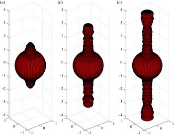
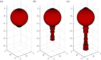
and producing two intersecting jets. Murphy et al. (Reference Murphy, Lery, O’Sullivan, Spicer, Bacciotti and Rosen2008) note that outflow from a system containing multiple protostars often involves only a single jet, and they undertook numerical simulation to account for the phenomenon. They conclude that the second jet is effectively absorbed into the main one, to the extent that it ceases to be readily visible. A similar result may be obtained in the present study, too, and such a case is discussed in § 5.
A truly fascinating instance of what appears to be interfacial outflow from a binary source system is evidently provided by the astrophysical object Eta Carinae, and this formed part of the initial motivation for undertaking the present work. This object has been the subject of intense study in the astrophysical literature, and a review of work until about the end of the twentieth century is given by Davidson & Humphreys (Reference Davidson and Humphreys1997). The system has an overall mass of perhaps 140 times that of our Sun, and is millions of times as luminous. In approximately 1844, it underwent a cataclysmic explosion, referred to as the ‘Great Eruption’, after which it became the second most bright star in the night sky for some years. During that time, it ejected in excess of
 $10\,\text{M}_{\odot }$
of material, creating a ‘Homunculus nebula’ that surrounds the inner region and obscures its view. This nebula consists of dust and ejected gas, forming two large osculating spheres such that the overall structure is approximately axisymmetric. A model that accounts for some features of the ‘Great Eruption’ of 1844 has been advanced by Smith (Reference Smith2013), and further details about the bipolar homunculus nebula and its composition are given by Steffen et al. (Reference Steffen, Teodoro, Madura, Groh, Gull, Mehner, Corcoran, Damineli and Hamaguchi2014). After some debate in the literature, the consensus is now that the Eta Carinae object most likely consists of two stars, one of about
 $110\,\text{M}_{\odot }$
and the other of perhaps
 $30\,\text{M}_{\odot }$
. They rotate about each other in a highly eccentric orbit, and each continues to eject a large volume of gas (hadrons) into the surrounding medium. The interaction of these stellar winds is the subject of very recent work by Clementel et al. (Reference Clementel, Madura, Kruip and Paardekooper2015). Fascinating recent work by Madura et al. (Reference Madura, Clementel, Gull, Kruip and Paardekooper2015) has modelled outflow from these orbiting binary stars using code based on smoothed-particle hydrodynamics, and formatting the three-dimensional output of this simulation to a 3D-printer. A very recent NASA website (NASA 2015) offers an animated view into the centre of Eta Carinae, based on observations and hydrodynamic simulations of the type presented by Madura et al. (Reference Madura, Clementel, Gull, Kruip and Paardekooper2015).
The present paper is a continuation of a sequence of investigations into fluid outflows from compact objects, and, motivated by astrophysical considerations, is focussed on the situation in which two point sources, located within a bubble of fluid of different density to its surrounds, are both ejecting mass. This is evidently the situation in an object such as Eta Carinae, where its two stars are ejecting hadrons into a more dense medium of dust and molecular hydrogen (Steffen et al. Reference Steffen, Teodoro, Madura, Groh, Gull, Mehner, Corcoran, Damineli and Hamaguchi2014). For simplicity, the two masses here are assumed to be stationary, allowing the simplifying approximation that the overall geometry is axisymmetric. Such a study may also be of interest in underwater explosions or in the injection of fluid into a reservoir, and so is of interest here also as a problem in fundamental fluid mechanics.
Since material ejected from the sources is of lower density than the surrounding fluid, the interface between them is subject to Rayleigh–Taylor instability. This type of flow is classical, and occurs when a horizontal layer of heavier fluid overlies a second layer of less dense fluid. The interface between them is unstable to small perturbations, which grow at a rate determined by the ratio of the densities of the two fluids. Forbes, Chen & Trenham (Reference Forbes, Chen and Trenham2007) developed a spectral solution technique for finding the evolving interface shape between layers of inviscid, incompressible fluid, and this was used by Forbes (Reference Forbes2009) to study nonlinear interfacial influences on the growth of the interface in classical planar Rayleigh–Taylor flow. A later study of planar outflow from a line sink (Forbes Reference Forbes2011a ) showed that, in this two-dimensional geometry, the initial conditions determined the shape that the interface would adopt at later times, although the initially cylindrical nature of the interface resulted in Bell–Plesset effects (Epstein Reference Epstein2004) due to its curvature, and these made stability considerations more complicated than just the Rayleigh–Taylor criterion. Initial conditions no longer determine the outflow shape in three-dimensional geometry, and Forbes (Reference Forbes2011b ) demonstrated that, instead, a one-sided jet is generated by outflow from a point source in the presence of an (initially spherical) interface. In a subsequent attempt to produce a two-sided, bipolar, outflow from a single point source in three-dimensional geometry, Forbes (Reference Forbes2014a ) included rotation and an external straining flow field, and demonstrated that two-sided outflows could indeed be generated by these mechanisms.
The present research is therefore motivated by the desire to determine whether strongly bipolar outflows are likely to be the result of including two (or more) sources within the initial bubble of less dense fluid in three-dimensional geometry, similar to the situation believed to occur within the Eta Carinae object (Madura et al. Reference Madura, Clementel, Gull, Kruip and Paardekooper2015). For planar flows involving two line sources, Forbes (Reference Forbes2014b ) has shown that outflows containing two jets do occur, but this gives no indication of the likely outflow morphology when two point sources in three-dimensional geometry are responsible for the flow. This question is addressed here for an initially spherical inner region of less dense fluid, in both the inviscid and a (Boussinesq) viscous model of the situation.
To begin, an inviscid, incompressible model of axisymmetric outflow from two point sources in an unbounded fluid system is first described. The sources emit fluid at some reference density into an outer fluid of different density, such that the two fluids are initially separated by a spherical surface. A method for the solution of this problem is developed in § 2, and is an extension of the spectral solution technique advanced by Forbes et al. (Reference Forbes, Chen and Trenham2007). A linearized theory is also possible in the inviscid case, assuming only small perturbations about the initially spherical shape of the interface, and gives a useful check on the reliability of the nonlinear results. This is described in § 3.
The effects of viscosity on these binary outflows are also included, and the viscous approach is outlined in § 4, using a Boussinesq approximation. A second aim of this paper is to develop a spectral solution technique for viscous fluids, that is capable of dealing exactly with the presence of two (or more) point singularities within the fluid, and the method for achieving this is outlined in § 4. Results are discussed in § 5, and they show that bipolar outflows are indeed possible, depending on the choice of parameters in the problem. One-sided jets are nevertheless still possible in this three-dimensional geometry, and they may develop ‘knots’ along their lengths. A brief discussion concludes the paper in § 6.
2. Inviscid fluid model
Consider a system of two fluids of different densities. An inner fluid of some finite volume sits in an initially spherical region of radius
 $a$
centred at the origin of a Cartesian coordinate system. This inner fluid has density
 ${\it\rho}_{1}$
. It is enclosed within a second fluid of unbounded extent, and having density
 ${\it\rho}_{2}$
. There is a sharp interface between these two fluids, across which the fluids are not free to mix.
Two heavy masses are present within the sphere of inner fluid 1 with density
 ${\it\rho}_{1}$
, and each has its own gravitational field. Mass number 1 is located at the point
 $(0,0,B)$
on the
 $z$
-axis and has mass
 $M_{1}$
. Furthermore, it ejects fluid of the same density
 ${\it\rho}_{1}$
isotropically at the volume flow rate
 $m_{1}$
. The second mass is also on the
 $z$
-axis at the opposite point
 $(0,0,-B)$
, with
 $B<a$
. This incurs no loss of generality, since the coordinate system can always be rotated and translated to ensure this is the case. This second object has mass
 $M_{2}$
and emits fluid of density
 ${\it\rho}_{1}$
at the rate
 $m_{2}$
(volume per time). Both fluids are assumed in this section to be incompressible and inviscid, so that they flow irrotationally.
Following Forbes (Reference Forbes2011b
, Reference Forbes2014a
), the problem is now recast in terms of spherical polar coordinates
 $(r,{\it\phi},{\it\theta})$
, in which
 $r$
is the radial distance from the origin,
 ${\it\phi}$
is the declination angle down from the
 $z$
-axis and
 ${\it\theta}$
is the azimuthal angle in the
 $xy$
-plane around the
 $z$
-axis. The relation between these and Cartesian coordinates is expressed in the usual formulae
 $$\begin{eqnarray}\displaystyle \left.\begin{array}{@{}rcl@{}}x\; & =\; & r\sin {\it\phi}\cos {\it\theta},\quad 0<r<\infty ,\\ y\; & =\; & r\sin {\it\phi}\sin {\it\theta},\quad \,0<{\it\phi}<{\rm\pi},\\ z\; & =\; & r\cos {\it\phi},\phantom{\sin {\it\theta}}\quad \,-{\rm\pi}<{\it\theta}<{\rm\pi},\end{array}\right\} & & \displaystyle\end{eqnarray}$$
which are given in Kreyszig (Reference Kreyszig2011, p. 594). Now the first mass is located at the point
 $(r,{\it\phi})=(B,0)$
and the second mass has position
 $(r,{\it\phi})=(B,{\rm\pi})$
independently of
 ${\it\theta}$
. The fluid velocity vector is written
 $\boldsymbol{q}=u\boldsymbol{e}_{r}+w\boldsymbol{e}_{{\it\phi}}+v\boldsymbol{e}_{{\it\theta}}$
, where the three unit vectors
 $\boldsymbol{e}_{r}$
,
 $\boldsymbol{e}_{{\it\phi}}$
and
 $\boldsymbol{e}_{{\it\theta}}$
point in the
 $r$
,
 ${\it\phi}$
and
 ${\it\theta}$
-directions, respectively. In this paper, the flow will be assumed to be axisymmetric, so that there is no dependence on the coordinate
 ${\it\theta}$
. In addition the azimuthal velocity component is taken to be zero;
 $v=0$
.
Non-dimensional coordinates are defined, and are used throughout this paper. The length scale is taken to be the initial radius
 $a$
of the sphere. An arbitrary reference flow rate
 $m_{R}$
(volume per time) is chosen, and then the time scale is
 $a^{3}/m_{R}$
and the scale for speed becomes
 $m_{R}/a^{2}$
. Pressures are then scaled relative to the quantity
 ${\it\rho}_{1}m_{R}^{2}/a^{4}$
, in which
 ${\it\rho}_{1}$
is the density in inner fluid 1. Velocity potential and streamfunction are both made dimensionless by reference to the quantity
 $m_{R}/a$
. Notice that, since the reference volume flow rate
 $m_{R}$
is arbitrary, it could be set to either of the quantities
 $m_{1}$
or
 $m_{2}$
already present in this problem, so eliminating the need for one of the dimensionless constants arising. However, it is preferable to allow the reference quantity
 $m_{R}$
to remain genuinely arbitrary, since this allows an obvious linearized solution to be developed, as outlined in § 3. This form of the non-dimensionalization now naturally leads to the presence of the six dimensionless constants
 $$\begin{eqnarray}\displaystyle \left.\begin{array}{@{}c@{}}\displaystyle F_{1}=\frac{m_{R}}{\sqrt{GM_{1}a^{3}}};\quad {\it\beta}=\frac{B}{a};\quad {\it\gamma}=\frac{M_{2}}{M_{1}},\\ \displaystyle D=\frac{{\it\rho}_{2}}{{\it\rho}_{1}};\quad {\it\eta}_{1}=\frac{m_{1}}{m_{R}};\quad {\it\eta}_{2}=\frac{m_{2}}{m_{R}}.\end{array}\right\} & & \displaystyle\end{eqnarray}$$
The first of these constants
 $F_{1}$
may be regarded as a Froude number based on the mass
 $M_{1}$
of the (upper) source, and
 $G$
in this expression is the gravitational constant. The quantity
 ${\it\beta}$
is now the dimensionless distance of each mass from the origin, and since these masses lie within the initial sphere of dimensionless radius
 $1$
containing the inner fluid, it follows that
 ${\it\beta}<1$
. The ratio of the two masses is
 ${\it\gamma}$
, and
 $D$
is the density ratio of the outer fluid to the inner one. Finally, the two dimensionless outflow strengths from the two masses are
 ${\it\eta}_{1}$
and
 ${\it\eta}_{2}$
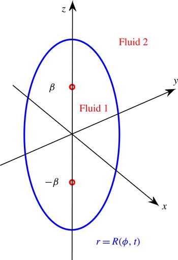
. These quantities could be either negative or positive, depending on whether these objects behave as sources or sinks. A sketch of the dimensionless flow situation is given in figure 1.
A sketch of the dimensionless configuration for the inviscid outflow from the two sources.

Since the two fluids are modelled in this section as being inviscid, they flow without rotation. Consequently, the velocity vector in the inner fluid may be written
 $\boldsymbol{q}_{1}=\boldsymbol{{\rm\nabla}}{\it\Phi}_{1}$
and similarly,
 $\boldsymbol{q}_{2}=\boldsymbol{{\rm\nabla}}{\it\Phi}_{2}$
for the fluid in the surrounding medium. The two functions
 ${\it\Phi}_{1}$
and
 ${\it\Phi}_{2}$
are velocity potentials in the inner and outer fluids, respectively. As each fluid is incompressible, it follows that each velocity potential satisfies Laplace’s equation
 ${\rm\nabla}^{2}{\it\Phi}_{j}=0$
,
 $j=1,2$
in its appropriate fluid domain. In inner fluid 1, there are two sources, and each of these is modelled as a mathematical point singularity for convenience. As a result, the velocity potential
 ${\it\Phi}_{1}$
near the top source must behave as
 $$\begin{eqnarray}{\it\Phi}_{1}\rightarrow -\frac{{\it\eta}_{1}}{4{\rm\pi}\sqrt{r^{2}-2{\it\beta}r\cos {\it\phi}+{\it\beta}^{2}}}\quad \text{as }(r,{\it\phi})\rightarrow ({\it\beta},0).\end{eqnarray}$$
Similarly, near the bottom source,
 $$\begin{eqnarray}{\it\Phi}_{1}\rightarrow -\frac{{\it\eta}_{2}}{4{\rm\pi}\sqrt{r^{2}+2{\it\beta}r\cos {\it\phi}+{\it\beta}^{2}}}\quad \text{as }(r,{\it\phi})\rightarrow ({\it\beta},{\rm\pi}).\end{eqnarray}$$
Between the two fluids, there is assumed to be an infinitesimally thin interface with the equation
 $r=\mathscr{R}({\it\phi},t)$
, as illustrated in figure 1. The fluid on each side of the interface does not cross it, and this is expressed by the two kinematic boundary conditions
 $$\begin{eqnarray}u_{j}=\frac{\partial \mathscr{R}}{\partial t}+\frac{w_{j}}{\mathscr{R}}\frac{\partial \mathscr{R}}{\partial {\it\phi}}\quad \text{on }r=\mathscr{R}({\it\phi},t),j=1,2\end{eqnarray}$$
at the interface. It is also necessary to impose a dynamical condition that the pressures either side of this interface must be equal. In each fluid, the pressure may be calculated from Bernoulli’s equation, which is a first integral of the Euler equations of motion (see Batchelor Reference Batchelor1967, § 3.5), and equating these pressures gives
 $$\begin{eqnarray}\displaystyle & & \displaystyle D\frac{\partial {\it\Phi}_{2}}{\partial t}-\frac{\partial {\it\Phi}_{1}}{\partial t}+\frac{1}{2}D(u_{2}^{2}+w_{2}^{2})-\frac{1}{2}(u_{1}^{2}+w_{1}^{2})\nonumber\\ \displaystyle & & \displaystyle \qquad -\,\frac{(D-1)}{F_{1}^{2}}\left[\frac{1}{\sqrt{r^{2}-2{\it\beta}r\cos {\it\phi}+{\it\beta}^{2}}}+\frac{{\it\gamma}}{\sqrt{r^{2}+2{\it\beta}r\cos {\it\phi}+{\it\beta}^{2}}}\right]\nonumber\\ \displaystyle & & \displaystyle \quad =f(t)\quad \text{on }r=\mathscr{R}({\it\phi},t).\end{eqnarray}$$
Here, the function
 $f(t)$
is arbitrary, and has no effect on the interface shape.
It follows (from separation of variables arguments) that velocity potentials in the two fluids may be written
 $$\begin{eqnarray}\displaystyle {\it\Phi}_{1}(r,{\it\phi},t) & = & \displaystyle -\frac{{\it\eta}_{1}}{4{\rm\pi}\sqrt{r^{2}-2{\it\beta}r\cos {\it\phi}+{\it\beta}^{2}}}-\frac{{\it\eta}_{2}}{4{\rm\pi}\sqrt{r^{2}+2{\it\beta}r\cos {\it\phi}+{\it\beta}^{2}}}\nonumber\\ \displaystyle & & \displaystyle +\,\mathop{\sum }_{n=1}^{N}B_{n}(t)r^{n}P_{n}(\cos {\it\phi})\end{eqnarray}$$
and
 $$\begin{eqnarray}\displaystyle {\it\Phi}_{2}(r,{\it\phi},t) & = & \displaystyle -\frac{{\it\eta}_{1}}{4{\rm\pi}\sqrt{r^{2}-2{\it\beta}r\cos {\it\phi}+{\it\beta}^{2}}}-\frac{{\it\eta}_{2}}{4{\rm\pi}\sqrt{r^{2}+2{\it\beta}r\cos {\it\phi}+{\it\beta}^{2}}}\nonumber\\ \displaystyle & & \displaystyle +\,\mathop{\sum }_{n=1}^{N}C_{n}(t)r^{-n-1}P_{n}(\cos {\it\phi}).\end{eqnarray}$$
These expressions become exact as the number of modes
 $N$
becomes infinite; however, numerical considerations require a finite value for
 $N$
. The unknown coefficient functions
 $B_{n}(t)$
and
 $C_{n}(t)$
are to be found. The interface shape is similarly expressed in the form
 $$\begin{eqnarray}\mathscr{R}({\it\phi},t)=A(t)+H_{0}(t)+\mathop{\sum }_{n=1}^{N}H_{n}(t)P_{n}(\cos {\it\phi}).\end{eqnarray}$$
The functions
 $P_{n}(z)$
in these expressions (2.7)–(2.9) are Legendre polynomials, as presented in Gradshteyn & Ryzhik (Reference Gradshteyn and Ryzhik2000, § 8.91). These polynomials and their derivatives may be generated efficiently from their three-term recurrence formulae, which are presented in Forbes (Reference Forbes2011b
) for these spherical coordinates. The coefficients
 $H_{0}(t)$
and
 $H_{n}(t)$
,
 $n=1,\ldots ,N$
, in (2.9) are to be determined, but the average time-dependent outflow radius has the known value
 $$\begin{eqnarray}A(t)=\left[1+\frac{3({\it\eta}_{1}+{\it\eta}_{2})t}{4{\rm\pi}}\right]^{1/3},\end{eqnarray}$$
which follows purely from considerations of mass balance. The series (2.7), (2.8) satisfy Laplace’s equation in their respective domains, and (2.7) also satisfies the singular behaviours (2.3), (2.4) near the two sources in the inner layer.
The unknown coefficient functions in (2.7)–(2.9) are determined using the first ‘basic’ solution scheme presented by Forbes et al. (Reference Forbes, Chen and Trenham2007). To begin, velocity components
 $U_{1}({\it\phi},t)$
,
 $W_{1}({\it\phi},t)$
and
 $U_{2}({\it\phi},t)$
,
 $W_{2}({\it\phi},t)$
are defined on the actual moving interface
 $r=\mathscr{R}({\it\phi},t)$
itself, by taking the vector gradients of the two potentials
 ${\it\Phi}_{1}$
and
 ${\it\Phi}_{2}$
in (2.7) and (2.8). Thus
 $$\begin{eqnarray}\displaystyle U_{1}({\it\phi},t) & = & \displaystyle \frac{\partial {\it\Phi}_{1}}{\partial r}\biggm\vert_{r=\mathscr{R}}\nonumber\\ \displaystyle & = & \displaystyle \frac{{\it\eta}_{1}(\mathscr{R}-{\it\beta}\cos {\it\phi})}{4{\rm\pi}[\mathscr{R}^{2}-2{\it\beta}\mathscr{R}\cos {\it\phi}+{\it\beta}^{2}]^{3/2}}+\frac{{\it\eta}_{2}(\mathscr{R}+{\it\beta}\cos {\it\phi})}{4{\rm\pi}[\mathscr{R}^{2}+2{\it\beta}\mathscr{R}\cos {\it\phi}+{\it\beta}^{2}]^{3/2}}\nonumber\\ \displaystyle & & \displaystyle +\,\mathop{\sum }_{n=1}^{N}nB_{n}(t)\mathscr{R}^{n-1}P_{n}(\cos {\it\phi})\end{eqnarray}$$
and
 $$\begin{eqnarray}\displaystyle W_{1}({\it\phi},t) & = & \displaystyle \frac{1}{r}\frac{\partial {\it\Phi}_{1}}{\partial {\it\phi}}\biggm\vert_{r=\mathscr{R}}\nonumber\\ \displaystyle & = & \displaystyle \frac{{\it\eta}_{1}{\it\beta}\sin {\it\phi}}{4{\rm\pi}[\mathscr{R}^{2}-2{\it\beta}\mathscr{R}\cos {\it\phi}+{\it\beta}^{2}]^{3/2}}-\frac{{\it\eta}_{2}{\it\beta}\sin {\it\phi}}{4{\rm\pi}[\mathscr{R}^{2}+2{\it\beta}\mathscr{R}\cos {\it\phi}+{\it\beta}^{2}]^{3/2}}\nonumber\\ \displaystyle & & \displaystyle -\,\mathop{\sum }_{n=1}^{N}B_{n}(t)\mathscr{R}^{n-1}P_{n}^{\prime }(\cos {\it\phi})\sin {\it\phi},\end{eqnarray}$$
and similar expressions apply for the two velocity components
 $U_{2}$
and
 $W_{2}$
at the interface, in outer fluid 2.
Now the first kinematic boundary condition, (2.5) with
 $j=1$
, is Fourier analysed using the orthogonality conditions for Legendre polynomials (these are given in Forbes (Reference Forbes2011b
) and Forbes (Reference Forbes2014a
) for spherical coordinates). This immediately yields the ordinary differential equations
 $$\begin{eqnarray}H_{0}^{\prime }(t)=-A^{\prime }(t)+\frac{1}{2}\int _{0}^{{\rm\pi}}\left[U_{1}-\frac{W_{1}}{\mathscr{R}}\frac{\partial \mathscr{R}}{\partial {\it\phi}}\right]\sin {\it\phi}\,\text{d}{\it\phi}\end{eqnarray}$$
and
 $$\begin{eqnarray}\displaystyle H_{\ell }^{\prime }(t)=\frac{(2\ell +1)}{2}\int _{0}^{{\rm\pi}}\left[U_{1}-\frac{W_{1}}{\mathscr{R}}\frac{\partial \mathscr{R}}{\partial {\it\phi}}\right]P_{\ell }(\cos {\it\phi})\sin {\it\phi}\,\text{d}{\it\phi},\quad \ell =1,\ldots ,N, & & \displaystyle\end{eqnarray}$$
for the coefficients in the expression (2.9) for the interface shape.
As in the method proposed by Forbes et al. (Reference Forbes, Chen and Trenham2007), the second kinematic condition with
 $j=2$
in the system (2.5) is replaced by the difference of the two, written as
 $$\begin{eqnarray}\mathscr{R}^{2}(U_{2}-U_{1})=(W_{2}-W_{1})\mathscr{R}\frac{\partial \mathscr{R}}{\partial {\it\phi}}.\end{eqnarray}$$
This equation is now subject to Fourier–Legendre decomposition. The zeroth-mode contribution is derived simply by multiplying by
 $\sin {\it\phi}$
and integrating, and after some algebra, is found to be satisfied identically. The contribution from the
 $\ell$
th Fourier mode is then obtained by multiplying by
 $P_{\ell }(\cos {\it\phi})\sin {\it\phi}$
and integrating. Integration by parts is used, along with the second-order differential equation satisfied by the Legendre polynomials (see Kreyszig Reference Kreyszig2011, p. 175), and leads to the elegant algebraic relations
 $$\begin{eqnarray}\mathop{\sum }_{n=1}^{N}S_{\ell n}^{(1)}B_{n}(t)+\mathop{\sum }_{n=1}^{N}S_{\ell n}^{(2)}C_{n}(t)=0,\quad \ell =1,\ldots ,N,\end{eqnarray}$$
between the two sets of Fourier coefficients
 $B_{n}(t)$
and
 $C_{n}(t)$
in the expressions (2.7), (2.8). In (2.16), the two sets of intermediate functions are
 $$\begin{eqnarray}\displaystyle \left.\begin{array}{@{}c@{}}\displaystyle S_{\ell n}^{(1)}(t)=\frac{1}{(n+1)}\int _{0}^{{\rm\pi}}\mathscr{R}^{n+1}({\it\phi},t)P_{n}^{\prime }(\cos {\it\phi})P_{\ell }^{\prime }(\cos {\it\phi})\,\sin ^{3}{\it\phi}\,\text{d}{\it\phi},\\ \displaystyle S_{\ell n}^{(2)}(t)=\frac{1}{n}\int _{0}^{{\rm\pi}}\mathscr{R}^{-n}({\it\phi},t)P_{n}^{\prime }(\cos {\it\phi})P_{\ell }^{\prime }(\cos {\it\phi})\,\sin ^{3}{\it\phi}\,\text{d}{\it\phi}.\end{array}\right\} & & \displaystyle\end{eqnarray}$$
Forbes et al. (Reference Forbes, Chen and Trenham2007) observed that, in spite of its elegance, an equation like (2.16) presents some difficulties, since it is a purely algebraic system. Differential equations, such as those in (2.13), (2.14), would be more easily accommodated within a numerical scheme, and can be derived from (2.16) directly, by differentiation. After some algebra, the desired differential relations are obtained in the final form
 $$\begin{eqnarray}\mathop{\sum }_{n=1}^{N}S_{\ell n}^{(1)}B_{n}^{\prime }(t)+\mathop{\sum }_{n=1}^{N}S_{\ell n}^{(2)}C_{n}^{\prime }(t)=-Q_{\ell }(t),\quad \ell =1,\ldots ,N,\end{eqnarray}$$
where the intermediate quantities
 $$\begin{eqnarray}Q_{\ell }(t)=\int _{0}^{{\rm\pi}}[W_{2}-W_{1}]\left[\mathscr{R}U_{1}-\frac{\partial \mathscr{R}}{\partial {\it\phi}}W_{1}\right]P_{\ell }^{\prime }(\cos {\it\phi})\sin ^{2}{\it\phi}\,\text{d}{\it\phi}\end{eqnarray}$$
have been defined for convenience.
It remains to satisfy the dynamic condition (2.6). The contribution from the
 $\ell$
th Fourier mode is again obtained by multiplying by
 $P_{\ell }(\cos {\it\phi})\sin {\it\phi}$
and integrating. The term involving the arbitrary function
 $f(t)$
vanishes under this process, which leads to the further system of differential equations
 $$\begin{eqnarray}\displaystyle D\mathop{\sum }_{n=1}^{N}K_{\ell n}^{(2)}C_{n}^{\prime }(t)-\mathop{\sum }_{n=1}^{N}K_{\ell n}^{(1)}B_{n}^{\prime }(t)=\frac{1}{2}J_{\ell }^{(1)}-\frac{1}{2}DJ_{\ell }^{(2)}+\frac{(D-1)}{F_{1}^{2}}Y_{\ell }, & & \displaystyle\end{eqnarray}$$
in which it is convenient to define the intermediate functions
 $$\begin{eqnarray}\displaystyle \left.\begin{array}{@{}c@{}}\displaystyle K_{\ell n}^{(1)}(t)=\int _{0}^{{\rm\pi}}\mathscr{R}^{n}P_{\ell }(\cos {\it\phi})P_{n}(\cos {\it\phi})\sin {\it\phi}\,\text{d}{\it\phi},\\ \displaystyle K_{\ell n}^{(2)}(t)=\int _{0}^{{\rm\pi}}\mathscr{R}^{-n-1}P_{\ell }(\cos {\it\phi})P_{n}(\cos {\it\phi})\sin {\it\phi}\,\text{d}{\it\phi},\\ \displaystyle J_{\ell }^{(1)}(t)=\int _{0}^{{\rm\pi}}(U_{1}^{2}+W_{1}^{2})P_{\ell }(\cos {\it\phi})\sin {\it\phi}\,\text{d}{\it\phi},\\ \displaystyle J_{\ell }^{(2)}(t)=\int _{0}^{{\rm\pi}}(U_{2}^{2}+W_{2}^{2})P_{\ell }(\cos {\it\phi})\sin {\it\phi}\,\text{d}{\it\phi},\end{array}\right\} & & \displaystyle\end{eqnarray}$$
and
 $$\begin{eqnarray}\displaystyle Y_{\ell }(t) & = & \displaystyle \int _{0}^{{\rm\pi}}\left[\frac{1}{\sqrt{\mathscr{R}^{2}-2{\it\beta}\mathscr{R}\cos {\it\phi}+{\it\beta}^{2}}}+\frac{{\it\gamma}}{\sqrt{\mathscr{R}^{2}+2{\it\beta}\mathscr{R}\cos {\it\phi}+{\it\beta}^{2}}}\right]\nonumber\\ \displaystyle & & \displaystyle \times \,P_{\ell }(\cos {\it\phi})\sin {\it\phi}\,\text{d}{\it\phi}.\end{eqnarray}$$
The sets of Fourier coefficients needed to construct the nonlinear time-dependent inviscid solution are now able to be calculated from these differential equations. The initial conditions are assumed simply to be that the interface starts as a sphere of dimensionless radius 1, with outflow from the two sources as given in (2.3) and (2.4). This gives the simple initial conditions
 $H_{0}(0)=0$
,
 $H_{n}(0)=0$
,
 $B_{n}(0)=C_{n}(0)=0$
,
 $n=1,\ldots ,N$
. Equations (2.13) and (2.14) now immediately give the derivatives
 $H_{0}^{\prime }$
and
 $H_{n}^{\prime }$
while (2.18) and (2.20) must be solved together as a matrix system, at each time step, to provide the derivatives
 $B_{n}^{\prime }$
and
 $C_{n}^{\prime }$
. This now results in a system of
 $3N+1$
ordinary differential equations, that are integrated forward in time using the MATLAB routine ode45, which is an accurate fourth/fifth order Runge–Kutta–Fehlberg solver, with adaptive time steps. The intermediate quantities (2.17), (2.19), (2.21) and (2.22) all involve quadratures, which have been evaluated to very high precision using the Gauss–Legendre routine lgwt written by von Winckel (Reference von Winckel2004).
3. Linearized inviscid solution
In order to carry out a linearized approximation to the outflow from the binary source system, it is necessary to assume that the two source strengths are small and the gravitational attraction effects are also small. To this end, we now set
 $$\begin{eqnarray}{\it\eta}_{1}={\it\epsilon}H_{1};\quad {\it\eta}_{2}={\it\epsilon}H_{2};\quad \frac{1}{F_{1}^{2}}={\it\epsilon}S_{1}\end{eqnarray}$$
for some small parameter
 ${\it\epsilon}$
. The two velocity potentials and the interface shape are now expressed as regular perturbation expansions in powers of
 ${\it\epsilon}$
, in the forms
 $$\begin{eqnarray}\displaystyle & {\it\Phi}_{1}(r,z,t)={\it\epsilon}\hat{P}_{1}(r,z,t)+O({\it\epsilon}^{2}), & \displaystyle\end{eqnarray}$$
 $$\begin{eqnarray}\displaystyle & {\it\Phi}_{2}(r,z,t)={\it\epsilon}\hat{P}_{2}(r,z,t)+O({\it\epsilon}^{2}), & \displaystyle\end{eqnarray}$$
 $$\begin{eqnarray}\displaystyle & \mathscr{R}(z,t)=1+{\it\epsilon}\hat{R}_{1}(r,z,t)+O({\it\epsilon}^{2}). & \displaystyle\end{eqnarray}$$
 ${\it\epsilon}$
can be regarded as giving a measure of the extent of the deformation of the interface from its initial spherical shape. Now the two kinematic conditions (2.5) give rise to the linearized expressions
 $$\begin{eqnarray}\frac{\partial \hat{P}_{1}}{\partial r}=\frac{\partial \hat{R}_{1}}{\partial t};\quad \frac{\partial \hat{P}_{2}}{\partial r}=\frac{\partial \hat{R}_{1}}{\partial t}\quad \text{on }r=1,\end{eqnarray}$$
and the dynamic condition (2.6) linearizes to
 $$\begin{eqnarray}\displaystyle & & \displaystyle D\frac{\partial \hat{P}_{2}}{\partial t}-\frac{\partial \hat{P}_{1}}{\partial t}=S_{1}(D-1)\left[\frac{1}{\sqrt{1-2{\it\beta}\cos {\it\phi}+{\it\beta}^{2}}}+\frac{{\it\gamma}}{\sqrt{1+2{\it\beta}\cos {\it\phi}+{\it\beta}^{2}}}\right]\nonumber\\ \displaystyle & & \displaystyle \quad \text{on }r=1.\end{eqnarray}$$
The expansion (3.2) and the approximate interface conditions (3.3), (3.4) show that this linearized problem will be equivalent, in some sense, to a small-time solution, since the interface is assumed not to deviate greatly from its initial spherical configuration
 $r=1$
.
Since the linearized velocity potentials must still satisfy Laplace’s equation and conditions (2.3), (2.4) at the two sources, it is appropriate to assume
 $$\begin{eqnarray}\displaystyle \hat{P}_{1}(r,{\it\phi},t) & = & \displaystyle -\frac{H_{1}}{4{\rm\pi}\sqrt{r^{2}-2{\it\beta}r\cos {\it\phi}+{\it\beta}^{2}}}-\frac{H_{2}}{4{\rm\pi}\sqrt{r^{2}+2{\it\beta}r\cos {\it\phi}+{\it\beta}^{2}}}\nonumber\\ \displaystyle & & \displaystyle +\,\mathop{\sum }_{n=1}^{\infty }\hat{B}_{n}(t)r^{n}P_{n}(\cos {\it\phi}),\quad r<1,\end{eqnarray}$$
and
 $$\begin{eqnarray}\displaystyle \hat{P}_{2}(r,{\it\phi},t) & = & \displaystyle -\frac{H_{1}}{4{\rm\pi}\sqrt{r^{2}-2{\it\beta}r\cos {\it\phi}+{\it\beta}^{2}}}-\frac{H_{2}}{4{\rm\pi}\sqrt{r^{2}+2{\it\beta}r\cos {\it\phi}+{\it\beta}^{2}}}\nonumber\\ \displaystyle & & \displaystyle +\,\mathop{\sum }_{n=1}^{\infty }{\hat{C}}_{n}(t)r^{-n-1}P_{n}(\cos {\it\phi}),\quad r>1,\end{eqnarray}$$
as for the nonlinear forms (2.7), (2.8). The linearized kinematic conditions (3.3) lead at once to the conclusion
 $$\begin{eqnarray}n\hat{B}_{n}(t)=-(n+1){\hat{C}}_{n}(t).\end{eqnarray}$$
The two forms (3.5) and (3.6) for the linearized velocity potentials and the relation (3.7) are now used in the linearized dynamic condition (3.4). The resulting equation is Fourier analysed, by multiplying by
 $P_{\ell }(\cos {\it\phi})\sin {\it\phi}$
and integrating, to give the contribution from the
 $\ell$
th mode. This gives
 $$\begin{eqnarray}\displaystyle & & \displaystyle \left[D+\frac{\ell +1}{\ell }\right]{\hat{C}}_{\ell }^{\prime }(t)\frac{2}{2\ell +1}\nonumber\\ \displaystyle & & \displaystyle \quad =S_{1}(D-1)\left[\int _{0}^{{\rm\pi}}\frac{P_{\ell }(\cos {\it\phi})\sin {\it\phi}\,\text{d}{\it\phi}}{\sqrt{1-2{\it\beta}\cos {\it\phi}+{\it\beta}^{2}}}+\int _{0}^{{\rm\pi}}\frac{{\it\gamma}P_{\ell }(\cos {\it\phi})\sin {\it\phi}\,\text{d}{\it\phi}}{\sqrt{1+2{\it\beta}\cos {\it\phi}+{\it\beta}^{2}}}\right]\!,\nonumber\\ \displaystyle & & \displaystyle \qquad \ell =1,\ldots ,N.\end{eqnarray}$$
The two integrals in this expression can be evaluated in closed form, using the generating functions for the Legendre polynomials (see Gradshteyn & Ryzhik Reference Gradshteyn and Ryzhik2000, p. 978) leading to
 $$\begin{eqnarray}\int _{0}^{{\rm\pi}}\frac{P_{\ell }(\cos {\it\phi})\sin {\it\phi}\,\text{d}{\it\phi}}{\sqrt{1-2{\it\beta}\cos {\it\phi}+{\it\beta}^{2}}}={\it\beta}^{\ell }\frac{2}{2\ell +1}.\end{eqnarray}$$
Equation (3.8) is now easily integrated with respect to time, and it follows from (3.7) that
 $$\begin{eqnarray}\displaystyle \left.\begin{array}{@{}c@{}}\displaystyle \hat{B}_{n}(t)=-tS_{1}(D-1)\frac{(n+1){\it\beta}^{n}[1+{\it\gamma}(-1)^{n}]}{Dn+(n+1)},\\ \displaystyle {\hat{C}}_{n}(t)=tS_{1}(D-1)\frac{n{\it\beta}^{n}[1+{\it\gamma}(-1)^{n}]}{Dn+(n+1)}.\end{array}\right\} & & \displaystyle\end{eqnarray}$$
When combined with the series forms (3.5), (3.6), these relations (3.10) give the complete forms for the two velocity potentials.
The interface shape is now available from (3.3), after a further integration with respect to time. Using the relations (3.1) to recover the original dimensionless parameters gives the linearized shape in the final form
 $$\begin{eqnarray}\displaystyle \mathscr{R}({\it\phi},t) & = & \displaystyle 1+\frac{t}{4{\rm\pi}}\left[\frac{{\it\eta}_{1}(1-{\it\beta}\cos {\it\phi})}{[1-2{\it\beta}\cos {\it\phi}+{\it\beta}^{2}]^{3/2}}+\frac{{\it\eta}_{2}(1+{\it\beta}\cos {\it\phi})}{[1+2{\it\beta}\cos {\it\phi}+{\it\beta}^{2}]^{3/2}}\right]\nonumber\\ \displaystyle & & \displaystyle -\,\frac{t^{2}(D-1)}{2F_{1}^{2}}\mathop{\sum }_{n=1}^{\infty }\frac{n(n+1){\it\beta}^{n}[1+{\it\gamma}(-1)^{n}]}{Dn+(n+1)}P_{n}(\cos {\it\phi})+O({\it\epsilon}^{2}).\end{eqnarray}$$
This expression (3.11) is evaluated numerically to good accuracy, typically by summing the first fifty or so terms in the series. Convergence is good, since
 ${\it\beta}<1$
.
Forbes (Reference Forbes2011b
) observed that outflow from a single source was most likely to occur as a one-sided jet, since that is the most unstable mode, and therefore the one that grows most rapidly and dominates all the others. Consequently, Forbes (Reference Forbes2014a
) was keen to explore situations that might lead to a more bipolar outflow shape, as is often observed in astrophysics. It is therefore appropriate to ask the same question of the linearized solution (3.11) in the present outflow geometry, with two point sources present. Mathematically, true bipolar symmetry requires
 $\mathscr{R}({\it\phi},t)=\mathscr{R}({\rm\pi}-{\it\phi},t)$
, and a necessary condition for this to occur is that the two source strengths should be equal;
 ${\it\eta}_{1}={\it\eta}_{2}$
. In addition, since
 $P_{n}(\cos ({\rm\pi}-{\it\phi}))=P_{n}(-\cos \,{\it\phi})$
, then it follows that bipolar symmetry will be possible only when the even-order Legendre polynomials alone are involved, since these possess just the even powers of their arguments. From (3.11), the odd-mode Legendre polynomials in the sum term cancel precisely when
 ${\it\gamma}=1$
only. Therefore, according to linearized theory, the outflow from the two-source system can only be symmetrically bipolar if the sources have equal strength,
 ${\it\eta}_{1}={\it\eta}_{2}$
, and the two masses are equal,
 ${\it\gamma}=1$
, and therefore have equal gravitational attraction. This accords with physical intuition.
4. Viscous fluid model
It is desirable also to understand the role of viscosity in the formation of these outflows, and that is done here using a Boussinesq formulation to simplify the problem. Such an approach was used by Forbes (Reference Forbes2011b , Reference Forbes2014a ) for the case of a single point source in axisymmetric three-dimensional flow, and has been generalized more recently by Forbes (Reference Forbes2014b ) to account for the presence of two line sources in planar two-dimensional flow. Here, the technique must be developed further to model the presence of two point sinks in axisymmetric outflow in three dimensions. Dimensionless variables are again used, as in § 2.
In the Boussinesq approximation, the fluid density
 ${\it\rho}$
is supposed to consist of its contribution
 ${\it\rho}=1$
from the inner fluid and the two point sources, and a small perturbation component
 $\bar{{\it\rho}}$
. Thus
 ${\it\rho}=1+\bar{{\it\rho}}$
and necessarily
 $\bar{{\it\rho}}=0$
in the inner fluid 1, and
 $\bar{{\it\rho}}=(D-1)$
in surrounding fluid 2. Since the density perturbation is small,
 $(D-1)$
must also be small. The Boussinesq approximation thus convects the density perturbation
 $\bar{{\it\rho}}$
around with the moving fluid, and as discussed in Forbes (Reference Forbes2014a
), this variable may alternatively be thought of as temperature, or perhaps even as a marker for salinity.
Crucially, the Boussinesq approximation ignores the presence of a mathematical interface of infinitesimal thickness between the two fluids, replacing it instead with an interfacial mixing zone of narrow, but finite, width. In its simplest form, Boussinesq theory thus considers the two-fluid system as just a single fluid of continuously-varying density, in which there is an interfacial zone, necessarily of finite thickness, across which the density varies rapidly but smoothly from its true value in the inner fluid to its corresponding value in the outer medium. This is done originally to simplify the algebra in the formulation of the problem, since the exact viscous conditions at the interface (see Batchelor Reference Batchelor1967, p. 150) can simply be ignored. Moore (Reference Moore1979) proved that, for inviscid fluids, the interface between them develops a curvature singularity within finite time, and Forbes (Reference Forbes2009) demonstrated numerically that this inviscid singularity is replaced by a small but finite region of very high vorticity in the viscous case, and this causes the interface to roll up as time progresses. However, it has been shown very recently by Forbes et al. (Reference Forbes, Paul, Chen and Horsley2015) that, even in the viscous case, a mathematical thin interface may still form curvature singularities within finite time, although by a different mechanism to the Moore (Reference Moore1979) curvature singularity at the interface between inviscid fluids. This surprising result was demonstrated asymptotically as well as numerically. So another major advantage of the Boussinesq approximation is that it happens to avoid all these difficulties, by dealing instead with a finite-width interfacial zone instead of a precise mathematical discontinuity.
In the Boussinesq approximation, the Navier–Stokes equations of viscous flow become
 $$\begin{eqnarray}\frac{\partial \boldsymbol{q}}{\partial t}+(\boldsymbol{q}\boldsymbol{\cdot }\boldsymbol{{\rm\nabla}})\boldsymbol{q}+\boldsymbol{{\rm\nabla}}p=-\frac{1}{F_{1}^{2}}(1+\bar{{\it\rho}})\boldsymbol{f}+\frac{1}{R_{e}}{\rm\nabla}^{2}\boldsymbol{q}.\end{eqnarray}$$
Here, the constant
 $R_{e}=({\it\rho}_{1}m_{R})/({\it\mu}a)$
is a Reynolds number based on the dimensional initial radius
 $a$
of the sphere, the dynamic viscosity
 ${\it\mu}$
and the (unspecified) reference volume flow rate
 $m_{R}$
as in § 2. The Froude number is again
 $F_{1}$
and
 $\boldsymbol{f}$
is the combined gravitational force per mass of the two sources. As in the work of Forbes (Reference Forbes2011b
), it is again convenient here to work with the vorticity
 ${\bf\zeta}=\text{curl}\,\boldsymbol{q}={\it\zeta}_{{\it\theta}}\boldsymbol{e}_{{\it\theta}}$
which only has the one component in the azimuthal
 ${\it\theta}$
-direction, for axisymmetric flow. In spherical polar coordinates, this vorticity component is given in terms of the velocity components as
 $$\begin{eqnarray}{\it\zeta}_{{\it\theta}}=\frac{1}{r}\left[\frac{\partial }{\partial r}(rw)-\frac{\partial u}{\partial {\it\phi}}\right].\end{eqnarray}$$
A vorticity equation is now derived by taking the vector curl of the Boussinesq Navier–Stokes equation (4.1). After some considerable algebra, the result is found to be
 $$\begin{eqnarray}\displaystyle & & \displaystyle \frac{\partial {\it\zeta}_{{\it\theta}}}{\partial t}+u\frac{\partial {\it\zeta}_{{\it\theta}}}{\partial r}+\frac{w}{r}\frac{\partial {\it\zeta}_{{\it\theta}}}{\partial {\it\phi}}-\frac{{\it\zeta}_{{\it\theta}}}{r}[u+w\cot {\it\phi}]\nonumber\\ \displaystyle & & \displaystyle \quad =\frac{1}{F_{1}^{2}[r^{2}-2{\it\beta}r\cos {\it\phi}+{\it\beta}^{2}]^{3/2}}\left[\frac{(r-{\it\beta}\cos {\it\phi})}{r}\frac{\partial \bar{{\it\rho}}}{\partial {\it\phi}}-{\it\beta}\sin {\it\phi}\frac{\partial \bar{{\it\rho}}}{\partial r}\right]\nonumber\\ \displaystyle & & \displaystyle \qquad +\,\frac{{\it\gamma}}{F_{1}^{2}[r^{2}+2{\it\beta}r\cos {\it\phi}+{\it\beta}^{2}]^{3/2}}\left[\frac{(r+{\it\beta}\cos {\it\phi})}{r}\frac{\partial \bar{{\it\rho}}}{\partial {\it\phi}}+{\it\beta}\sin {\it\phi}\frac{\partial \bar{{\it\rho}}}{\partial r}\right]\nonumber\\ \displaystyle & & \displaystyle \qquad +\,\frac{1}{R_{e}}\left[\frac{1}{r^{2}}\frac{\partial }{\partial r}\left(r^{2}\frac{\partial {\it\zeta}_{{\it\theta}}}{\partial r}\right)+\frac{1}{r^{2}\sin {\it\phi}}\frac{\partial }{\partial {\it\phi}}\left(\sin {\it\phi}\frac{\partial {\it\zeta}_{{\it\theta}}}{\partial {\it\phi}}\right)-\frac{{\it\zeta}_{{\it\theta}}}{r^{2}\sin ^{2}{\it\phi}}\right].\end{eqnarray}$$
Many of the terms in this equation may be checked against the similar expressions given in Batchelor (Reference Batchelor1967, p. 601).
In the Boussinesq approximation, the mass conservation equation is ‘split’ into an essentially incompressible part and a transport equation for the density perturbation
 $\bar{{\it\rho}}$
, to give the two equations
 $$\begin{eqnarray}\displaystyle \left.\begin{array}{@{}c@{}}\displaystyle \text{div}\,\boldsymbol{q}=0,\\ \displaystyle \frac{\partial \bar{{\it\rho}}}{\partial t}+\boldsymbol{q}\boldsymbol{\cdot }\boldsymbol{{\rm\nabla}}\bar{{\it\rho}}={\it\sigma}{\rm\nabla}^{2}\bar{{\it\rho}}.\end{array}\right\} & & \displaystyle\end{eqnarray}$$
The first of the conditions in the system (4.4) is satisfied identically by making use of a streamfunction
 ${\it\Psi}(r,{\it\phi},t)$
, in terms of which the two velocity components may be written
 $$\begin{eqnarray}u=\frac{1}{r\sin {\it\phi}}\frac{\partial }{\partial {\it\phi}}({\it\Psi}\sin {\it\phi});\quad w=-\frac{1}{r}\frac{\partial }{\partial r}(r{\it\Psi}).\end{eqnarray}$$
The two functions to be found in this formulation are therefore the density perturbation
 $\bar{{\it\rho}}$
and the streamfunction
 ${\it\Psi}$
, and they are the solutions to the vorticity equation (4.3) and the transport equation in the system (4.4).
A spectral representation for these two functions is now sought. An artificial ‘computational boundary’ is introduced at some spherical surface
 $r=R$
, and the aim is then to create a representation for the streamfunction
 ${\it\Psi}$
that gives a similar form for the vorticity component
 ${\it\zeta}_{{\it\theta}}$
. After some algebra, the appropriate form is found to be
 $$\begin{eqnarray}\displaystyle {\it\Psi}(r,{\it\phi},t) & = & \displaystyle \frac{{\it\eta}_{1}({\it\beta}-r\cos {\it\phi})}{4{\rm\pi}r\sin {\it\phi}\sqrt{r^{2}-2r{\it\beta}\cos {\it\phi}+{\it\beta}^{2}}}-\frac{{\it\eta}_{2}({\it\beta}+r\cos {\it\phi})}{4{\rm\pi}r\sin {\it\phi}\sqrt{r^{2}+2r{\it\beta}\cos {\it\phi}+{\it\beta}^{2}}}\nonumber\\ \displaystyle & & \displaystyle +\,\mathop{\sum }_{m=1}^{M}\mathop{\sum }_{n=1}^{N}A_{mn}(t)\frac{1}{\sqrt{r}}\text{J}_{n+1/2}({\it\alpha}_{nm}r)P_{n}^{\prime }(\cos {\it\phi})\sin {\it\phi}.\end{eqnarray}$$
In this expression, the function
 $\text{J}_{n+1/2}$
is the first-kind Bessel function of order
 $n+1/2$
and is related to the spherical Bessel functions (see Abramowitz & Stegun Reference Abramowitz and Stegun1972, p. 360). The function
 $P_{n}$
is the Legendre polynomial of degree
 $n$
(Gradshteyn & Ryzhik Reference Gradshteyn and Ryzhik2000, § 8.91) and
 $P_{n}^{\prime }$
is its derivative. Expressions similar to (4.6) were used by Forbes (Reference Forbes2011b
, Reference Forbes2014a
). The additional constants appearing in this representation are defined to be
 $$\begin{eqnarray}{\it\alpha}_{nm}=j_{n+1/2,m}/R,\end{eqnarray}$$
in which the symbol
 $j_{n+1/2,m}$
denotes the
 $m$
th zero of the Bessel function
 $\text{J}_{n+1/2}$
. These have been calculated here using the simple bisection method and asymptotic estimates for these zeros given in Abramowitz & Stegun (Reference Abramowitz and Stegun1972, p. 371). The task is to calculate the time-dependent Fourier coefficients
 $A_{mn}(t)$
in this representation (4.6).
It follows from (4.5) that the two velocity components now become
 $$\begin{eqnarray}\displaystyle u(r,{\it\phi},t) & = & \displaystyle \frac{{\it\eta}_{1}(r-{\it\beta}\cos {\it\phi})}{4{\rm\pi}[r^{2}-2r{\it\beta}\cos {\it\phi}+{\it\beta}^{2}]^{3/2}}+\frac{{\it\eta}_{2}(r+{\it\beta}\cos {\it\phi})}{4{\rm\pi}[r^{2}+2r{\it\beta}\cos {\it\phi}+{\it\beta}^{2}]^{3/2}}\nonumber\\ \displaystyle & & \displaystyle +\,\mathop{\sum }_{m=1}^{M}\mathop{\sum }_{n=1}^{N}n(n+1)A_{mn}(t)\frac{1}{r^{3/2}}\text{J}_{n+1/2}({\it\alpha}_{nm}r)P_{n}(\cos {\it\phi})\end{eqnarray}$$
and
 $$\begin{eqnarray}\displaystyle & & \displaystyle w(r,{\it\phi},t)=\frac{{\it\eta}_{1}{\it\beta}\sin {\it\phi}}{4{\rm\pi}[r^{2}-2r{\it\beta}\cos {\it\phi}+{\it\beta}^{2}]^{3/2}}-\frac{{\it\eta}_{2}{\it\beta}\sin {\it\phi}}{4{\rm\pi}[r^{2}+2r{\it\beta}\cos {\it\phi}+{\it\beta}^{2}]^{3/2}}\nonumber\\ \displaystyle & & \displaystyle \quad -\,\mathop{\sum }_{m=1}^{M}\mathop{\sum }_{n=1}^{N}A_{mn}(t)\left[\frac{1}{2r^{3/2}}\text{J}_{n+1/2}({\it\alpha}_{nm}r)+\frac{{\it\alpha}_{nm}}{\sqrt{r}}\text{J}_{n+1/2}^{\prime }({\it\alpha}_{nm}r)\right]P_{n}^{\prime }(\cos {\it\phi})\sin {\it\phi}.\end{eqnarray}$$
These two velocity components with (4.2) give
 $$\begin{eqnarray}{\it\zeta}_{{\it\theta}}(r,{\it\phi},t)=\mathop{\sum }_{m=1}^{M}\mathop{\sum }_{n=1}^{N}A_{mn}(t)\frac{{\it\alpha}_{nm}^{2}}{\sqrt{r}}\text{J}_{n+1/2}({\it\alpha}_{nm}r)P_{n}^{\prime }(\cos {\it\phi})\sin {\it\phi}\end{eqnarray}$$
as the final form for the representation of the vorticity component.
A spectral representation is also needed for the density perturbation function
 $\bar{{\it\rho}}$
. The selection of an appropriate form turns out to be a difficult problem, and all the more so in this case because of the two point sources located within inner fluid 1. For the case of planar flow with two line sources, Forbes (Reference Forbes2014b
) coped with this difficulty by multiplying the governing equations by functions that vanished at the locations of the two line sources; this is adequate for solving the problem, but possibly may not give an entirely faithful representation of the density perturbation function at the sources themselves. Accordingly, it seemed preferable here to use a form
 $$\begin{eqnarray}\displaystyle & & \displaystyle \bar{{\it\rho}}(r,{\it\phi},t)=(D-1)\mathscr{H}(r,{\it\phi})\nonumber\\ \displaystyle & & \displaystyle \quad \times \,\left[1+\mathop{\sum }_{m=1}^{M}C_{m0}(t)\cos ({\it\alpha}_{0m}r)+\mathop{\sum }_{m=1}^{M}\mathop{\sum }_{n=1}^{N}C_{mn}(t)\frac{1}{\sqrt{r}}\text{J}_{n+1/2}({\it\alpha}_{nm}r)P_{n}(\cos {\it\phi})\right],\qquad\end{eqnarray}$$
since this representation can satisfy exactly the condition that
 $\bar{{\it\rho}}=0$
at the locations of the two point sources in this problem. Here, additional constants
 $$\begin{eqnarray}{\it\alpha}_{0m}=(2m-1){\rm\pi}/(2R)\end{eqnarray}$$
have been defined for convenience. It is necessary to choose the function
 $\mathscr{H}(r,{\it\phi})$
in (4.11) carefully, both to satisfy the requirements that the density perturbation should be zero at the two source points as well as to become
 $1$
at large radius
 $r$
, so as to avoid numerical ill conditioning and give the correct value
 $\bar{{\it\rho}}\rightarrow (D-1)$
far away. An appropriate choice is therefore
 $$\begin{eqnarray}\mathscr{H}(r,{\it\phi})=\frac{[r^{2}-2{\it\beta}r\cos {\it\phi}+{\it\beta}^{2}][r^{2}+2{\it\beta}r\cos {\it\phi}+{\it\beta}^{2}]}{[r^{2}+{\it\beta}^{2}]^{2}}.\end{eqnarray}$$
It now turns out that, with this choice (4.13) for the function
 $\mathscr{H}$
in the representation (4.11) for the density perturbation function, no further manipulation of the governing equations is needed in the spectral solution method. However, the presence of the function
 $\mathscr{H}$
in (4.11) effectively means that the basis functions in the spectral solution for
 $\bar{{\it\rho}}$
are no longer orthogonal.
The representation (4.10) is substituted into the vorticity equation (4.3), and the resulting expression is Fourier decomposed, by multiplying by
 $$\begin{eqnarray}r^{3/2}\text{J}_{\ell +1/2}({\it\alpha}_{\ell k}r)P_{\ell }^{\prime }(\cos {\it\phi})\sin ^{2}{\it\phi}\end{eqnarray}$$
and integrating over the domain
 $0<r<R$
,
 $0<{\it\phi}<{\rm\pi}$
. The derivatives
 $P_{n}^{\prime }$
of the Legendre polynomials obey an orthogonality condition, which is given by Forbes (Reference Forbes2011b
) in these spherical coordinates. The Bessel functions
 $\text{J}_{n+1/2}$
are also orthogonal with respect to the weight function
 $r$
and so a set of ordinary differential equations is obtained, for the unknown coefficients
 $A_{mn}(t)$
. For completeness, these are given in the appendix A.
The expression (4.11) is similarly substituted into the transport equation for
 $\bar{{\it\rho}}$
, the second in the system (4.4). The resulting equation is lengthy, primarily due to the Laplacian term
 ${\it\sigma}{\rm\nabla}^{2}\bar{{\it\rho}}$
on the right-hand side and the presence of the additional function
 $\mathscr{H}$
in (4.11). A zeroth Fourier-mode contribution in
 ${\it\phi}$
is first derived by multiplying by
 $\cos ({\it\alpha}_{0k}r)\sin {\it\phi}$
and integrating. This gives a set of
 $M$
differential equations of the general form
 $$\begin{eqnarray}\displaystyle \mathop{\sum }_{m=1}^{M}\mathscr{M}_{m0k0}C_{m0}^{\prime }(t)+\mathop{\sum }_{m=1}^{M}\mathop{\sum }_{n=1}^{N}\mathscr{N}_{mnk0}C_{mn}^{\prime }(t)=R_{k0},\quad k=1,\ldots ,M, & & \displaystyle\end{eqnarray}$$
in which the constants
 $\mathscr{M}_{m0k0}$
and so on are presented in the appendix A. Higher Fourier-mode contributions are similarly obtained by multiplying the density transport equation in (4.4) by
 $$\begin{eqnarray}r^{3/2}\text{J}_{\ell +1/2}({\it\alpha}_{\ell k}r)P_{\ell }(\cos {\it\phi})\sin {\it\phi}\end{eqnarray}$$
and integrating, as before. This results in a further set of differential equations with the general forms
 $$\begin{eqnarray}\displaystyle \mathop{\sum }_{m=1}^{M}\mathscr{M}_{m0k\ell }C_{m0}^{\prime }(t)+\mathop{\sum }_{m=1}^{M}\mathop{\sum }_{n=1}^{N}\mathscr{N}_{mnk\ell }C_{mn}^{\prime }(t)=R_{k\ell },\quad k=1,\ldots ,M,\ell =1,\ldots ,N,\quad & & \displaystyle\end{eqnarray}$$
in which the constants
 $\mathscr{M}_{m0k\ell }$
and so on are again given in the appendix A.
This system of
 $M(N+1)$
differential equations (4.15), (4.17) is set up as an
 $M(N+1)\times M(N+1)$
linear matrix equation for a vector containing all the derivatives
 $C_{m0}^{\prime }(t)$
,
 $C_{mn}^{\prime }(t)$
and must first be solved for these derivatives at each new time step. In fact, the coefficient matrix is independent of time
 $t$
, and so only needs to be inverted once, and its inverse cached in memory at the beginning of the algorithm. In this way, although the basis functions for the representation of
 $\bar{{\it\rho}}$
in (4.11) are no longer orthogonal, in practice this does not incur too great an additional numerical cost.
Now the system of
 $M(2N+1)$
differential equations (A 1), (4.15) and (4.17) is integrated forward in time, using the MATLAB routine ode45, as in § 2. There are many quantities in these expressions involving terms defined in terms of integrals, as is evident from (A 1), (A 6) and (A 7) in the appendix A. These quadratures are all evaluated numerically, using the Gaussian routine lgwt written by von Winckel (Reference von Winckel2004). It has been found that making use of
 $121$
mesh points in
 $r$
and the same number in
 ${\it\phi}$
enables these quadratures to be performed to very high accuracy. Results are typically obtained with
 $M=N=31$
coefficients, and as demonstrated by Forbes (Reference Forbes2014a
), this gives sufficient accuracy to resolve the features of interest in these evolving outflows.
The initial condition is chosen to mimic that used for the inviscid solution in §§ 2 and 3. The initial velocity is just that due to the presence of the two sources, and thus the coefficients in the series for streamfunction are set initially to zero, so that
 $$\begin{eqnarray}A_{k\ell }(0)=0,\quad k=1,\ldots ,M,\ell =1,\ldots ,N.\end{eqnarray}$$
The density perturbation function is initially zero inside the unit sphere and
 $(D-1)$
outside it, so that the condition
 $$\begin{eqnarray}\bar{{\it\rho}}(r,{\it\phi},0)=\left\{\begin{array}{@{}ll@{}}0\quad & \text{if }r<1,\\ (D-1)\quad & \text{if }r>1,\end{array}\right.\end{eqnarray}$$
must be satisfied. In order to impose this initial condition (4.19), the representation (4.11) must be subject to Fourier decomposition, as previously. This leads to the system of algebraic equations
 $$\begin{eqnarray}\displaystyle & & \displaystyle \mathop{\sum }_{m=1}^{M}\mathscr{M}_{m0k0}C_{m0}(0)+\mathop{\sum }_{m=1}^{M}\mathop{\sum }_{n=1}^{N}\mathscr{N}_{mnk0}C_{mn}(0)=\int _{0}^{R}\int _{0}^{{\rm\pi}}\left[\frac{\bar{{\it\rho}}(r,{\it\phi},0)}{(D-1)}-\mathscr{H}\right]\nonumber\\ \displaystyle & & \displaystyle \quad \times \,\cos ({\it\alpha}_{0k}r)\sin {\it\phi}\,\text{d}{\it\phi}\,\text{d}r,\quad k=1,\ldots ,M,\end{eqnarray}$$
and
 $$\begin{eqnarray}\displaystyle & & \displaystyle \mathop{\sum }_{m=1}^{M}\mathscr{M}_{m0k\ell }C_{m0}(0)+\mathop{\sum }_{m=1}^{M}\mathop{\sum }_{n=1}^{N}\mathscr{N}_{mnk\ell }C_{mn}(0)=\int _{0}^{R}\int _{0}^{{\rm\pi}}\left[\frac{\bar{{\it\rho}}(r,{\it\phi},0)}{(D-1)}-\mathscr{H}\right]\nonumber\\ \displaystyle & & \displaystyle \quad \times \,r^{3/2}\text{J}_{\ell +1/2}({\it\alpha}_{\ell k}r)P_{\ell }(\cos {\it\phi})\sin {\it\phi}\,\text{d}{\it\phi}\,\text{d}r,\quad k=1,\ldots ,M,\ell =1,\ldots ,N.\end{eqnarray}$$
These expressions involve further quadratures, which are again evaluated using the Gaussian routine lgwt written by von Winckel (Reference von Winckel2004). However, the left-hand sides of these two equations (4.20), (4.21) have the same algebraic structure as the differential equations (4.15), (4.17), and involve precisely the same sets of constants. Accordingly, the inverse of the large
 $M(N+1)\times M(N+1)$
matrix already calculated and stored at the beginning of the algorithm can again be used to solve this linear matrix equation system (4.20), (4.21) for the initial values of the coefficients
 $C_{m0}(0)$
,
 $C_{mn}(0)$
in the representation of the density perturbation.
5. Discussion of results
The algorithms for generating nonlinear solutions to the inviscid and viscous models, discussed in §§ 2 and 4, have been tested extensively across a wide range of parameter values, to assess the behaviour of the solution at different values and to confirm convergence of the results at different numbers of Fourier coefficients. Due to the spherical nature of the interface, it turns out that there is no particular difference in the results for
 $D<1$
and
 $D>1$
. This is because, in this geometry, it is not just the Rayleigh–Taylor instability influencing the outcome, but also the Bell–Plesset instability due to the curvature of the interface itself (see Epstein Reference Epstein2004). In order to simplify the presentation of results, therefore, only a density ratio
 $D=1.05$
will be considered here, in which the surrounding fluid is 5 % heavier than inner fluid 1. Similarly, the role of the Froude number
 $F_{1}$
in the results is largely to affect the time scale over which features evolve, and so just the single value
 $F_{1}=10$
will be discussed.
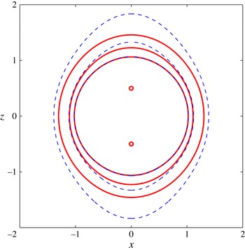
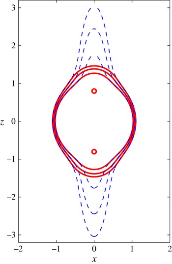
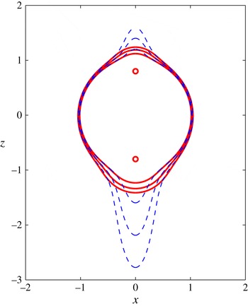
A comparison of the growth of the interface in the inviscid model, for the linearized (dashed; blue online) and nonlinear (heavy solid line; red online) theories. Solutions are shown at the three different times
 $t=2$
,
 $10$
and
 $30$
. The source location parameter is
 ${\it\beta}=0.5$
and their strengths are
 ${\it\eta}_{1}={\it\eta}_{2}=0.1$
. The two masses are equal, so
 ${\it\gamma}=1$
. The two small circles (red online) give the source locations.

Figure 2 gives a comparison of inviscid results, for the nonlinear algorithm discussed in § 2 and the linearized solution of § 3. The nonlinear solutions are drawn with heavy solid lines and the linearized results are indicated with lighter dashed lines. At the early time
 $t=2$
there is almost complete agreement between the two theories, as is evident in the figure. However the linearized theory, which is predicated on the assumption that the interface remains close to the initial sphere
 $r=1$
, progressively overestimates the extent of the outflow, and particularly near the poles of the original sphere, close to the
 $z$
-axis. In this sense, the linearized theory can be thought of as an early-time approximation in this instance, as suggested in § 3. Nevertheless, there is still reasonable agreement over most of the interface away from the two polar regions, and this is evident in the profiles at the intermediate time
 $t=10$
.
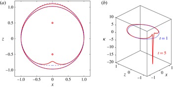
Evolution of the interface in the inviscid model at two different times
 $t=1$
and
 $5$
. The source location parameter is
 ${\it\beta}=0.5$
and the upper source has strength
 ${\it\eta}_{1}=0.1$
while the strength of the lower sink is
 ${\it\eta}_{2}=-0.1$
. The two masses are equal, so
 ${\it\gamma}=1$
. (a) Interface location for the linearized (dashed; blue online) and nonlinear (heavy solid line; red online) theories. The two small circles (red online) give the source locations. (b) Interfacial curvatures.

From the mathematical point of view, it is possible to consider the situation in which one of the sources within the jacket of the inner fluid region has negative strength, and so becomes a point sink, even if the relevance of such a calculation to astrophysics is questionable. For interest, such a situation is illustrated in figure 3. In these pictures, the solution is shown for
 ${\it\eta}_{1}=0.1$
,
 ${\it\eta}_{2}=-0.1$
so that the top singularity is a source that ejects fluid, but the bottom one is a sink that removes fluid at the same volume rate. Overall, there is no nett production of fluid so that, on average, the interface location would be expected to remain as
 $r=1$
. Again the masses are equal so that
 ${\it\gamma}=1$
and the location of the two singularities is
 ${\it\beta}=0.5$
.
Figure 3(a) illustrates the two interface profiles at the two times
 $t=1$
and
 $t=5$
, for both the linearized and nonlinear theories. The linearized predictions are drawn with dashed lines and the nonlinear results are indicated by thicker solid lines. The two theories are essentially indistinguishable at time
 $t=1$
. However, at the later time
 $t=5$
, the linearized theory again overpredicts the outflow near the upper source, and particularly so in the vicinity of the pole of the initial sphere on the upper portion of the
 $z$
-axis. By contrast, near the lower point, which is a sink, the linearized theory underestimates the extent to which the interface in the inviscid theory is pulled upwards on the diagram, towards the lower sink.
The sudden withdrawal of the interface toward the sink is a phenomenon dominated by nonlinear effects, as was originally demonstrated by Tuck & Vanden-Broeck (Reference Tuck and Vanden-Broeck1984) and more recently in unsteady selective withdrawal flows by Stokes et al. (Reference Stokes, Hocking and Forbes2003), for example. Forbes & Hocking (Reference Forbes and Hocking2007) showed that withdrawal into a drain is ultimately limited by the apparent formation of curvature singularities at the interface, in inviscid flow, similar in many respects to the Moore curvature singularity (Moore Reference Moore1979). This appears to be true in the present situation, too. Figure 3(b) shows the interfacial curvatures
 ${\it\kappa}$
for the two solutions in figure 3(a), at the two times
 $t=1$
and
 $t=5$
. These have been calculated from the formula
 $$\begin{eqnarray}{\it\kappa}=\frac{\mathscr{R}^{2}+2\mathscr{R}_{{\it\phi}}^{2}-\mathscr{R}\mathscr{R}_{{\it\phi}{\it\phi}}}{(\mathscr{R}^{2}+\mathscr{R}_{{\it\phi}}^{2})^{3/2}},\end{eqnarray}$$
which may be derived in spherical polar coordinates (2.1) from the formula for curvature given by Kreyszig (Reference Kreyszig2011, p. 392). One of the advantages of the spectral technique presented in § 2 is that a difficult quantity such as the curvature in (5.1) can be calculated to very high accuracy by exact differentiation of the representation (2.9) for the nonlinear interface
 $r=\mathscr{R}({\it\phi},t)$
; this was used by Forbes et al. (Reference Forbes, Paul, Chen and Horsley2015) to predict a curvature singularity in viscous Kelvin–Helmholtz flow, that was later confirmed analytically.
It may be seen from figure 3(b) that the interfacial curvature
 ${\it\kappa}$
at the early time
 $t=1$
is approximately constant, at the value
 ${\it\kappa}\approx 1$
, consistently with the interface lying on a sphere of unit radius. However, at the later time
 $t=5$
, a sharp negative spike of curvature has formed directly below the sink, at the point on the lower portion of the
 $z$
-axis. This spike forms rapidly as time progresses, and in fact the result shown was the last time for which the numerical method could give a solution. It therefore appears to be the case that the solution with a sink is ultimately limited by the formation of a curvature singularity within finite time, as the interface is drawn in toward the sink.
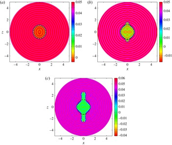
Evolution of the outflow in the viscous model at the three times (a)
 $t=4$
, (b)
 $t=10$
and (c)
 $t=13$
. The source location parameter is
 ${\it\beta}=0.5$
and the two sources have strengths
 ${\it\eta}_{1}={\it\eta}_{2}=0.1$
. The two masses are equal, so
 ${\it\gamma}=1$
. Contours of the density perturbation
 $\bar{{\it\rho}}$
are shown. The heavy dashed lines are the nonlinear inviscid predictions at each time.

The predictions of the viscous model in § 4 are now investigated, for the same case as shown in figure 2 for the inviscid case. The result is displayed in figure 4. The two sources have equal strengths
 ${\it\eta}_{1}={\it\eta}_{2}=0.1$
and they are located at half the initial radius of the sphere, so that
 ${\it\beta}=0.5$
. Their masses are equal;
 ${\it\gamma}=1$
. Viscous outflows are shown at the three different times
 $t=4$
,
 $t=10$
and
 $t=13$
, and consist of contour diagrams for the density perturbation function
 $\bar{{\it\rho}}$
at these three times. In the outer region, representing fluid 2 in figure 1, the density perturbation has the value
 $\bar{{\it\rho}}=0.05$
. The slightly mottled appearance of the shaded contours in this region is caused by the presence of waves of very small amplitude; these are numerical in origin, and are a consequence of Gibbs’ phenomenon (see Kreyszig Reference Kreyszig2011, p. 515) associated with the discontinuity in the initial condition (4.19) and are of no significance.
Also shown on the diagrams in figure 4 are the predictions of the nonlinear inviscid solution for the interface shape
 $r=\mathscr{R}({\it\phi},t)$
at the three times. These inviscid results are drawn with heavy dashed lines on each diagram. The viscous and inviscid results are clearly in very good agreement at early times. Thus the inviscid interface for time
 $t=4$
in figure 4(a) lies precisely within the narrow interfacial zone in the viscous solution, where the density function
 $\bar{{\it\rho}}$
changes smoothly but rapidly, as is evident from that picture. At later times, an interesting qualitative difference emerges, however, between the predictions of these two models. In the inviscid theory, the interface continues to grow in a nearly spherical shape, except for slight bulges near the two poles on the
 $z$
-axis. Such behaviour was also encountered in figure 2. On the other hand, the viscous model indicates that, while growth also begins this way for earlier times, there comes a time when small nodules appear near the two poles of the sphere, and these then grow rapidly outwards. Thus, in figure 4(b), while there is still reasonably good agreement between the viscous and inviscid predictions as to the location and shape of the interfacial zone at time
 $t=10$
, there are two small ‘buds’ that have developed in the viscous solution near the poles. These then grow rapidly, so that a short time later, they have developed into the pronounced bipolar jets in figure 4(c) at time
 $t=13$
. The rapid development of these jets is a significant challenge to numerical solution techniques, and the result for
 $t=13$
is the largest time for which these viscous solutions could be computed at this value of the source location parameter
 ${\it\beta}$
.
Perspective view of the interface for the viscous solution at time
 $t=13$
, for the case
 ${\it\beta}=0.5$
and source strengths
 ${\it\eta}_{1}={\it\eta}_{2}=0.1$
. The two masses are equal, so
 ${\it\gamma}=1$
.

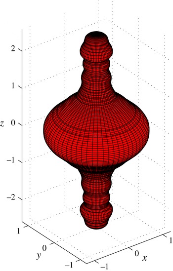
Figure 5 shows the effective interface for the viscous solution at time
 $t=13$
, displayed in figure 4(c). This diagram serves as a reminder that these outflows are indeed three dimensional, although axisymmetric. The interfacial surface in this picture was created by taking the contour
 $\bar{{\it\rho}}=0.02$
in figure 4(c) and rotating it about the
 $z$
-axis. The scales on all three axes are the same, so that the outflow jets are as they would actually appear. Smaller secondary waves along the jets are visible in this image, and represent a type of viscous Kelvin–Helmholtz instability, with small toroidal vortices formed in the outer fluid surrounding each jet.
Contours of the vorticity for the viscous solution at time
 $t=13$
, for the case
 ${\it\beta}=0.5$
and source strengths
 ${\it\eta}_{1}={\it\eta}_{2}=0.1$
. The two masses are equal, so
 ${\it\gamma}=1$
. The two small circles (red online) give the source locations.

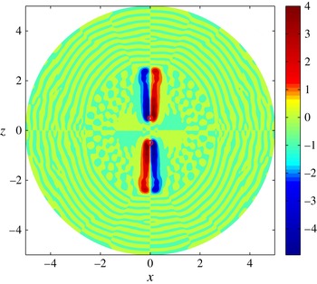
It is interesting to study the evolution of the vorticity function
 ${\it\zeta}_{{\it\theta}}$
in the outflow, and this is shown for the same parameters as in figures 4 and 5, at the last time
 $t=13$
for which viscous solutions could be found. In a study of the Rayleigh–Taylor instability, Forbes (Reference Forbes2009) demonstrated that the flow was essentially irrotational everywhere, except for relatively small regions near the interface, where vorticity was generated through viscous shear. Similar observations were made in relation to the one-sided outflow jets produced by a single point source (Forbes Reference Forbes2011b
, Reference Forbes2014a
). Figure 6 shows that a similar situation applies here, too. The vorticity is largely zero throughout the fluid, except in a narrow jacket around each outflow jet. This accounts for the very different outflow shapes between the inviscid and viscous solutions at later times.
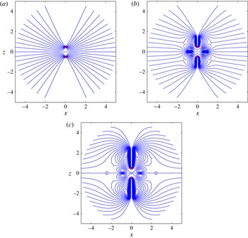
Evolution of streamlines in the viscous model at the three times (a)
 $t=4$
, (b)
 $t=10$
and (c)
 $t=13$
. The source location parameter is
 ${\it\beta}=0.5$
and the two sources have strengths
 ${\it\eta}_{1}={\it\eta}_{2}=0.1$
. The two masses are equal, so
 ${\it\gamma}=1$
. The two small circles on the
 $z$
-axis at
 $z=\pm 0.5$
(red online) give the source locations.

The development of the outflow jets may also be understood through a study of the streamsurfaces associated with the flow. Since the flow is axisymmetric, it has a streamfunction
 ${\it\Psi}$
, given by the expression (4.6). It is straightforward to prove that level surfaces of the function
 $$\begin{eqnarray}r\sin {\it\phi}\,{\it\Psi}(r,{\it\phi},t)\end{eqnarray}$$
are streamsurfaces for the flow, since tangents to these level surfaces are parallel to the fluid velocity vector.
Figure 7 illustrates the evolution of the streamlines on the plane
 $y=0$
, for the same flow discussed in figures 4–6, at the three times
 $t=4$
,
 $10$
and
 $13$
. The function in (5.2) was created from the spectral representation (4.6) and contoured at
 $21$
equally-spaced levels. Cartesian
 $x$
and
 $z$
were then created and plotted in figure 7. The scales on the axes are equal, and the locations of the two sources are indicated by small circles. At the early time
 $t=4$
in figure 7(a), the streamline pattern is clearly dominated by the two sources; there is a plane of symmetry at
 $z=0$
and each source produces the classical streamline pattern associated with a source placed next to the effective wall at this plane of symmetry. As time progresses, however, this pattern changes markedly, with the development of additional secondary vortices around the two jets. These are clearly visible in figure 7(b,c) at times
 $t=10$
and
 $13$
, and are responsible to a large extent for the shape of the outflows.
A comparison of the growth of the interface in the inviscid model, for the linearized (dashed; blue online) and nonlinear (heavy solid line; red online) theories. Solutions are shown at the three different times
 $t=4$
,
 $8$
and
 $12$
. The source location parameter is
 ${\it\beta}=0.8$
and their strengths are
 ${\it\eta}_{1}={\it\eta}_{2}=0.1$
. The two masses are equal, so
 ${\it\gamma}=1$
. The two small circles (red online) give the source locations.

The behaviour of the outflow jets is strongly affected by the locations
 ${\it\beta}$
of the two sources. Since the sources are located within the initial sphere of unit radius, it follows that
 ${\it\beta}<1$
, and as
 ${\it\beta}$
approaches
 $1$
, the outflow jets develop a more focussed, narrow shape. The inviscid situation for the case
 ${\it\beta}=0.8$
is illustrated in figure 8. Here, the predictions of the linearized theory in § 3 are drawn with dashed lines at the three different times
 $t=4$
,
 $8$
and
 $12$
. The nonlinear inviscid interface
 $r=\mathscr{R}({\it\phi},t)$
calculated from § 2 at the same three times is overlaid, using heavier solid lines. The agreement between the two theories is reasonably good over much of the interface, at all three times shown, except near the top and bottom poles of the original sphere, where the linearized theory very strongly overestimates the extent of the outflow, at least in the context of the inviscid model. It turns out, however, that the nonlinear viscous model also produces elongated outflow jets near the two poles, although they are much sharper and more focussed that the inviscid linearized solutions in figure 8. The viscous predictions are now investigated in figure 9.
Perspective view of the evolution of the interface for the viscous solution at the three times (a)
 $t=4$
, (b)
 $t=8$
and (c)
 $t=12$
. The source location parameter is
 ${\it\beta}=0.8$
and the two sources have strengths
 ${\it\eta}_{1}={\it\eta}_{2}=0.1$
. The two masses are equal, so
 ${\it\gamma}=1$
.

The outflow for two equal sources of strength
 ${\it\eta}_{1}={\it\eta}_{2}=0.1$
and source location parameter
 ${\it\beta}=0.8$
is shown for the viscous case in figure 9, at the three different times
 $t=4$
,
 $8$
and
 $12$
. After this time, the numerical algorithm of § 4 could not continue further. The scales on these axes are all equal, so that the shapes are as they would actually be seen, and each diagram has been drawn to the same size, so that they can be viewed relative to one another. Each picture has been created from a contour map of the density perturbation function
 $\bar{{\it\rho}}$
by locating the contour
 $\bar{{\it\rho}}=0.02$
and then rotating it about the
 $z$
-axis.
At the somewhat early time
 $t=4$
in figure 9(a), the shape is still largely spherical of approximately unit radius, although outflow nodules have already begun to form at the poles, above the two point sources. By time
 $t=8$
, shown in figure 8(b), those nodules have developed into pronounced outflow jets, symmetrical about the equatorial plane
 $z=0$
. They possess small secondary waves, associated with the presence of vortices surrounding the jets, similar to those seen in figure 7(c). At the last time
 $t=12$
shown in figure 9(c), the bipolar outflow jets have now developed further, forming long thin pencil-like jets with secondary wavelets. The central sphere-shaped region has actually decreased slightly in volume, as more fluid is pushed out to the rapidly expanding jets. Computing such structures is a challenge for a numerical technique, and solutions for
 $t$
significantly larger than
 $12$
have not been computed. Thus the ultimate fate of this solution for very large time remains unknown, but it is possible that the central spherical region may continue to shrink, and that the jets might become unstable and detach from it, and the whole cycle start again. At present, these fascinating morphological questions remain unanswered.
A comparison of the growth of the interface in the inviscid model, for the linearized (dashed; blue online) and nonlinear (heavy solid line; red online) theories. Solutions are shown at the three different times
 $t=1$
,
 $2$
and
 $3$
. The source location parameter is
 ${\it\beta}=0.8$
and the strengths are unequal, with
 ${\it\eta}_{1}=0.1$
and
 ${\it\eta}_{2}=0.3$
. The two masses are equal, so
 ${\it\gamma}=1$
. The two small circles (red online) give the source locations.

It is of interest now to see the effects of asymmetry on these outflows from two sources, in the viscous model. This could be achieved by replacing one of the sources with a sink, as in the inviscid case presented in figure 3, but in the viscous case the withdrawal of the finite-width interfacial zone into the sink is difficult to resolve, and so is not pursued here. Similarly, the two masses could be made unequal, so that
 ${\it\gamma}\neq 1$
, but it turns out that this makes only slight changes to the results, and is likewise not discussed further here, in the interests of space. By far the most interesting situation is that in which one of the sources is much stronger than the other, since much greater asymmetry is produced in this case, as is perhaps to be expected. Such a situation is illustrated for the inviscid model in figure 10. Here, the upper source on the diagram still has strength
 ${\it\eta}_{1}=0.1$
but the lower source now has
 ${\it\eta}_{2}=0.3$
. As for the symmetric cases shown in figures 2 and 8, the linearized solution very significantly overestimates the extent of the inviscid outflow near the sources, although it agrees very closely with the nonlinear result elsewhere along the interface. This is particularly evident near the lower, stronger, source in figure 10, where the pronounced bulge predicted by the linearized solution is not matched by the fully nonlinear inviscid result.
Perspective view of the evolution of the interface for the viscous solution at the three times (a)
 $t=1$
, (b)
 $t=2$
and (c)
 $t=3$
. The source location parameter is
 ${\it\beta}=0.8$
and the two sources have unequal strengths, with
 ${\it\eta}_{1}=0.1$
and
 ${\it\eta}_{2}=0.3$
. The two masses are equal, so
 ${\it\gamma}=1$
.

The predictions of the nonlinear viscous model are shown in figure 11, for the same parameters as the inviscid solution shown in previous figure 10, and for the same three times
 $t=1$
,
 $2$
and
 $3$
. The scale on the axes in the three pictures is the same, and each diagram has been drawn to be of the same size, to enable comparison. The three pictures were drawn by extracting the contour
 $\bar{{\it\rho}}=0.02$
from maps of the density perturbation function
 $\bar{{\it\rho}}(r,{\it\phi},t)$
at the three times, and then revolving that contour about the
 $z$
-axis. Once again, the upper source in these pictures has strength
 ${\it\eta}_{1}=0.1$
but the lower source is three times that strength, with
 ${\it\eta}_{2}=0.3$
. The effect of this asymmetry in source strengths has an intriguing effect on the evolution of the outflow shape, as can be seen in figure 11. Now an essentially one-sided outflow is generated, and looks at least superficially similar to the one-sided outflows produced by a single point source, discussed in Forbes (Reference Forbes2011b
), although the underlying reason for that shape in this case is very different.
At the early time
 $t=1$
depicted in figure 11(a), the outflow shape is almost just the initial sphere of unit radius, except that a small bump is present at the bottom of the ‘interfacial’ surface
 $\bar{{\it\rho}}=0.02$
below the lower source. At the later time
 $t=2$
in figure 11(b), that bump has now developed into a pronounced outflow jet towards the bottom of the picture. In fact, the contour
 $\bar{{\it\rho}}=0.02$
has actually pinched off to form a separate disconnected little surface at the bottom of the jet, although this may not be evident from figure 11(b). As time continues, the single jet grows longer and the final picture in figure 11(c) at the last time
 $t=3$
now features a very long jet with a somewhat complicated shape that contains a number of smaller cylindrical waves around its axis. Indeed, the bottom three ripples visible at the end of the jet in figure 11(c) for the contour
 $\bar{{\it\rho}}=0.02$
have all detached from the main jet and have had to be drawn separately, although this may again not be apparent from the diagram. Solutions for this case at later times have not been pursued, since the rapid development of the one-sided jet means that it is approaching the edge of the computational region, at the ‘artificial boundary’
 $R=5$
. To continue much beyond this time would require very greatly increased computer resources, since this boundary would have to be moved further out, necessitating in turn far more Fourier modes in the spectral solution representations (4.11) and so on, and many more mesh points for the accurate evaluation of the integrals in the spectral solution technique. As discussed in relation to figure 9 in the symmetrical case, the eventual fate of the one-sided outflow in figure 11 is likewise unknown at this time, although it is to be expected that the jet will continue to elongate, possibly with more and more detached segments as it does so.
6. Conclusion
When a single point source is placed in a surrounding fluid, and the source ejects fluid of a different density to its surroundings, the interface between the two fluids has been found to be unstable to the lowest mode, in axisymmetric geometry. This was shown earlier by Forbes (Reference Forbes2011b ), and the practical consequence is that a one-sided outflow jet is the most likely result. This is a surprising conclusion, and is not matched in the two-dimensional flow situation in which a line source ejects less dense fluid into a more dense medium (Forbes Reference Forbes2011a ). Nevertheless, one-sided ejecta have been observed in astrophysics by Gómez et al. (Reference Gómez, Rodríguez and Loinard2013) and are also reported in computational astrophysics, when an artificial constraint of symmetry about the centre plane is not imposed (Lovelace et al. Reference Lovelace, Romanova, Lii and Dyda2014).
Since bipolar outflows are often observed in astrophysics, for example (see Stahler & Palla Reference Stahler and Palla2004), it is natural to ask whether such structures might be produced by a binary pair of sources, and this has been the focus of the present research. Inviscid theory shows that, when the two sources are of identical mass and strength, a genuinely symmetrical outflow is indeed produced. A linearized solution has been presented in the inviscid case, and it agrees well with the nonlinear inviscid results, except near the regions of the two outflows, where it tends to exaggerate the size of the outflow region. Interestingly, when viscosity is introduced into the model, through a Boussinesq approximation, it is found that the outflow regions are in fact much more pronounced than the nonlinear inviscid theory allows; in that regard they are superficially similar to the linearized inviscid theory, although their structure is quite different. In addition, sources of very different strength can produce one-sided outflows, as shown in figure 11, and this may have relevance to the findings of Murphy et al. (Reference Murphy, Lery, O’Sullivan, Spicer, Bacciotti and Rosen2008).
The introduction of a second source within the region of the less dense fluid poses new numerical challenges. These have been addressed in this paper by the use of a novel spectral method in which the perturbation to the fluid density is made to vanish exactly at the two sources, so enforcing exactly the correct value of the density at those two points. This has only a minor effect on the buoyancy term in the vorticity (4.3), but it means that the basis functions in the spectral method are no longer orthogonal when applied to the density transport equation in the system (4.4). However, this difficulty is overcome here by storing the inverse of a matrix of the inner products of the basis functions, once at the beginning of the numerical algorithms, and then using it at each time step to integrate the density perturbation forward in time. Consequently, the computational cost of using such non-orthogonal basis functions is minimized. No difficulty has been encountered in this work with issues of ill conditioning that might arise from the non-orthogonality of the basis functions in the representation (4.11), (4.13) for density, with the two sources studied here. In principle, this new approach could be adapted to account for any number of sources within the fluid, although it may be that additional sources could indeed introduce numerical ill conditioning in the corresponding representation for density.
While the motivation for the present study has notionally involved astrophysical applications, it is nevertheless the case that this represents a canonical problem in fundamental fluid mechanics. It could, therefore, equally well apply to underwater explosions or inflows to reservoirs, for example. It should be possible to generalize such a study to account for additional effects such as magnetic forces or perhaps compressibility, as well as the influence of additional sources, and these are currently under investigation.
Acknowledgements
This work has been carried out in association with ARC (Australian Research Council) discovery grant DP140100094. I am indebted to Dr S. Walters for assistance with some of the figures. Constructive comments from three anonymous referees are gratefully acknowledged.
Appendix A. Differential equations for Boussinesq Fourier coefficients
The vorticity (4.3) is subject to Fourier decomposition, as detailed in § 4. This results in a system of equations for the time derivatives of the coefficients
 $A_{mn}(t)$
. After some algebra, that system is
 $$\begin{eqnarray}\displaystyle A_{k\ell }^{\prime }(t) & = & \displaystyle -\frac{1}{R_{e}}{\it\alpha}_{\ell k}^{2}A_{k\ell }(t)\nonumber\\ \displaystyle & & \displaystyle -\,\frac{1}{{\it\Delta}_{k\ell }}\int _{0}^{R}\int _{0}^{{\rm\pi}}\sqrt{r}\left[ru\frac{\partial {\it\zeta}_{{\it\theta}}}{\partial r}+w\frac{\partial {\it\zeta}_{{\it\theta}}}{\partial {\it\phi}}\right]\text{J}_{\ell +1/2}({\it\alpha}_{\ell k}r)P_{\ell }^{\prime }(\cos {\it\phi})\sin ^{2}{\it\phi}\,\text{d}{\it\phi}\,\text{d}r\nonumber\\ \displaystyle & & \displaystyle +\,\frac{1}{{\it\Delta}_{k\ell }}\int _{0}^{R}\int _{0}^{{\rm\pi}}\sqrt{r}{\it\zeta}_{{\it\theta}}[u\sin {\it\phi}+w\cos {\it\phi}]\text{J}_{\ell +1/2}({\it\alpha}_{\ell k}r)P_{\ell }^{\prime }(\cos {\it\phi})\sin {\it\phi}\,\text{d}{\it\phi}\,\text{d}r\nonumber\\ \displaystyle & & \displaystyle +\,\frac{1}{F_{1}^{2}{\it\Delta}_{k\ell }}\int _{0}^{R}\int _{0}^{{\rm\pi}}\sqrt{r}\frac{\mathscr{G}_{M}}{Z_{M}^{3/2}}\text{J}_{\ell +1/2}({\it\alpha}_{\ell k}r)P_{\ell }^{\prime }(\cos {\it\phi})\sin ^{2}{\it\phi}\,\text{d}{\it\phi}\,\text{d}r\nonumber\\ \displaystyle & & \displaystyle +\,\frac{{\it\gamma}}{F_{1}^{2}{\it\Delta}_{k\ell }}\int _{0}^{R}\int _{0}^{{\rm\pi}}\sqrt{r}\frac{\mathscr{G}_{P}}{Z_{P}^{3/2}}\text{J}_{\ell +1/2}({\it\alpha}_{\ell k}r)P_{\ell }^{\prime }(\cos {\it\phi})\sin ^{2}{\it\phi}\,\text{d}{\it\phi}\,\text{d}r,\nonumber\\ \displaystyle & & \displaystyle \quad k=1,\ldots ,M,\ell =1,\ldots ,N,\end{eqnarray}$$
where
 $$\begin{eqnarray}\displaystyle \mathscr{G}_{M}(r,{\it\phi},t)=(r-{\it\beta}\cos {\it\phi})\frac{\partial \bar{{\it\rho}}}{\partial {\it\phi}}-{\it\beta}r\sin {\it\phi}\frac{\partial \bar{{\it\rho}}}{\partial r}, & & \displaystyle\end{eqnarray}$$
 $$\begin{eqnarray}\displaystyle \mathscr{G}_{P}(r,{\it\phi},t)=(r+{\it\beta}\cos {\it\phi})\frac{\partial \bar{{\it\rho}}}{\partial {\it\phi}}+{\it\beta}r\sin {\it\phi}\frac{\partial \bar{{\it\rho}}}{\partial r}. & & \displaystyle\end{eqnarray}$$
 ${\it\Delta}_{k\ell }$
in (A 1) come from the orthogonality relations for the derivatives of the Legendre polynomials and for the Bessel functions, and are defined to be
 $$\begin{eqnarray}{\it\Delta}_{k\ell }=R^{2}{\it\alpha}_{\ell k}^{2}\text{J}_{\ell +3/2}^{2}({\it\alpha}_{\ell k}R)\frac{\ell (\ell +1)}{(2\ell +1)}.\end{eqnarray}$$
There are also two functions in (A 1) that arise from the function defined in (4.13); these are
 $$\begin{eqnarray}\displaystyle \left.\begin{array}{@{}c@{}}Z_{M}(r,{\it\phi})=r^{2}-2{\it\beta}r\cos {\it\phi}+{\it\beta}^{2},\\ Z_{P}(r,{\it\phi})=r^{2}+2{\it\beta}r\cos {\it\phi}+{\it\beta}^{2},\end{array}\right\} & & \displaystyle\end{eqnarray}$$
and these are chosen to vanish at the upper and lower source points, respectively.
A further set of differential equations (4.15), (4.17) is obtained after Fourier decomposition of the density transport equation, as detailed in § 4. These expressions involve a large number of intermediate constants, expressed as integrals. In (4.15), these constants are
 $$\begin{eqnarray}\displaystyle \mathscr{M}_{m0k0}=\int _{0}^{R}\int _{0}^{{\rm\pi}}\mathscr{H}\cos ({\it\alpha}_{0m}r)\cos ({\it\alpha}_{0k}r)\sin {\it\phi}\,\text{d}{\it\phi}\,\text{d}r, & & \displaystyle\end{eqnarray}$$
 $$\begin{eqnarray}\displaystyle \mathscr{N}_{mnk0}=\int _{0}^{R}\int _{0}^{{\rm\pi}}\mathscr{H}\frac{1}{\sqrt{r}}\text{J}_{n+1/2}({\it\alpha}_{nm}r)P_{n}(\cos {\it\phi})\cos ({\it\alpha}_{0k}r)\sin {\it\phi}\,\text{d}{\it\phi}\,\text{d}r, & & \displaystyle\end{eqnarray}$$
 $$\begin{eqnarray}\displaystyle R_{k0}=\int _{0}^{R}\int _{0}^{{\rm\pi}}\left[-\frac{1}{(D-1)}\left(u\frac{\partial \bar{{\it\rho}}}{\partial r}+\frac{w}{r}\frac{\partial \bar{{\it\rho}}}{\partial {\it\phi}}\right)+{\it\sigma}\mathscr{L}_{D}\right]\cos ({\it\alpha}_{0k}r)\sin {\it\phi}\,\text{d}{\it\phi}\,\text{d}r. & & \displaystyle\end{eqnarray}$$
In the last of these quantities, the symbol
 $\mathscr{L}_{D}$
represents the Laplacian of the function
 $\bar{{\it\rho}}$
in (4.11), but is not given here in the interests of space. The similar constants arising from (4.17) are
 $$\begin{eqnarray}\displaystyle \mathscr{M}_{m0k\ell }=\int _{0}^{R}\int _{0}^{{\rm\pi}}\mathscr{H}r^{3/2}\text{J}_{\ell +1/2}({\it\alpha}_{\ell k}r)\cos ({\it\alpha}_{0m}r)P_{\ell }(\cos {\it\phi})\sin {\it\phi}\,\text{d}{\it\phi}\,\text{d}r, & & \displaystyle\end{eqnarray}$$
 $$\begin{eqnarray}\displaystyle \mathscr{N}_{mnk\ell }=\int _{0}^{R}\int _{0}^{{\rm\pi}}\mathscr{H}r\text{J}_{n+1/2}({\it\alpha}_{nm}r)\text{J}_{\ell +1/2}({\it\alpha}_{\ell k}r)P_{n}(\cos {\it\phi})P_{\ell }(\cos {\it\phi})\sin {\it\phi}\,\text{d}{\it\phi}\,\text{d}r, & & \displaystyle\end{eqnarray}$$
 $$\begin{eqnarray}\displaystyle R_{k\ell } & = & \displaystyle \int _{0}^{R}\int _{0}^{{\rm\pi}}\left[-\frac{1}{(D-1)}\left(u\frac{\partial \bar{{\it\rho}}}{\partial r}+\frac{w}{r}\frac{\partial \bar{{\it\rho}}}{\partial {\it\phi}}\right)+{\it\sigma}\mathscr{L}_{D}\right]\nonumber\\ \displaystyle & & \displaystyle \times \,r^{3/2}\text{J}_{\ell +1/2}({\it\alpha}_{\ell k}r)P_{\ell }(\cos {\it\phi})\sin {\it\phi}\,\text{d}{\it\phi}\,\text{d}r.\end{eqnarray}$$