1 Introduction
In this work, we study the uniform computational strength of theorems arising in classical descriptive set theory related to perfect subsets of Polish spaces. In general, if P is a subset of a topological space
 $\mathcal {X}$
, a point
 $x \in P$
is a limit point of P if for every open set U with
 $x \in U$
there is a distinct point
 $y \in P \cap U$
: otherwise, we call x isolated in P. A subset of a topological space is perfect if it is closed and has no isolated points. An equivalent formulation is that
 $P\subseteq \mathcal {X}$
is perfect if
 $P=P'$
, where
 $P'$
is the Cantor–Bendixson derivative, i.e., the set of all limit points of P. Notice that every nonempty perfect subset of a Polish space has the cardinality of the continuum.
A classical theorem in this context is the Cantor–Bendixson theorem.
Theorem 1.1 (Cantor–Bendixson theorem).
Every closed subset C of a Polish space
 $\mathcal {X}$
can be uniquely written as the disjoint union of a perfect set P and a countable set S. We call P the perfect kernel of C and S the scattered part of C.
When
 $\mathcal {X}$
is either Cantor space
 $2^{\mathbb {N}}$
or Baire space
 $\mathbb {N}^{\mathbb {N}}$
, there is a well-known correspondence between closed sets and sets of paths through trees. In these settings, the Cantor–Bendixson theorem states that all but countably many paths through a tree T on
 $\mathbb {N}$
belong to a perfect subtree S of T (i.e., a tree such that every node has two incomparable extensions). Again, S (which is unique) is called the perfect kernel of T and the set of missing paths is the scattered part of T.
Many theorems in “classical” mathematics, including Theorem 1.1 and its tree version, can be written in the form
 $$\begin{align*}(\forall x \in X)(\varphi(x)\implies (\exists y \in Y)\psi(x,y)),\end{align*}$$
and this formulation has a natural translation as a computational problem: given an instance
 $x \in X$
satisfying
 $\varphi (x)$
, the task is to find a solution
 $y \in Y$
such that
 $\psi (x,y)$
(notice that such a y, in general, is not unique). A computational problem can be naturally rephrased as a (partial) multi-valued function
 ${{f}} :\subseteq {X} \rightrightarrows {Y}$
where
 $f(x):=\{y \in Y:\psi (x,y)\}$
, for every
 $x \in X$
such that
 $\varphi (x)$
. The interpretation of theorems as multi-valued functions/problems allows us to compare their uniform computational content using the framework of Weihrauch reducibility.
This work continues the program initiated by Gherardi and the second author [Reference Gherardi and Marcone12] that aims to provide a bridge between computable analysis and reverse mathematics, the discipline which establishes equivalences between mathematical statements and the axioms required to prove them. A well-known empirical fact in this field is the so-called big five phenomenon. Namely, many theorems of “classical” mathematics happen to be equivalent to one of five subsystems of second-order arithmetic, namely
 $\mathsf {RCA}_0,\mathsf {WKL}_0,\mathsf {ACA}_0,\mathsf {ATR}_0$
, and
 $\boldsymbol {\Pi }^1_1{-}\mathsf{CA}_0$
. Some analogs of the big five have been identified in the Weihrauch context. For example,
 $\mathsf {RCA}_0$
roughly corresponds to computable problems,
 $\mathsf {WKL}_0$
to the task of choosing an element from a nonempty closed subset of the Cantor space (denoted by
 $\mathsf {C}^{\mathsf {\vphantom {g}}}_{{2^{\mathbb {N}}}} $
), and
 $\mathsf {ACA}_0$
to iterations of
 $\mathsf {lim}$
, where
 $\mathsf {lim}$
is the problem that takes in input a converging sequence in Baire space and outputs its limit.
The second author in [Reference Brattka, Kawamura, Marcone and Pauly9] raised the question “What do the Weihrauch hierarchies look like once we go to very high levels of reverse mathematics strength?”. Here we continue to answer this question by focusing on theorems that, in reverse mathematics, are either equivalent to
 $\mathsf {ATR}_0$
or
 $\boldsymbol {\Pi }^1_1{-}\mathsf{CA}_0$
. In this direction, it has been shown that statements that in reverse mathematics are equivalent to
 $\mathsf {ATR}_0$
, when considered as problems, fall into different Weihrauch degrees (see for example [Reference Anglès d’Auriac and Kihara1, Reference Kihara, Marcone and Pauly15–Reference Le Goh17, Reference Marcone and Valenti19]). On the other hand,
 $\boldsymbol {\Pi }^1_1{-}\mathsf{CA}_0$
has a natural correspondent in the Weihrauch lattice, namely the problem
 $\widehat {\mathsf {WF}}$
that given in input a sequence of trees on
 $\mathbb {N}$
outputs the sequence
 $p \in 2^{\mathbb {N}}$
such that
 $p(i)=1$
iff the i-th tree of the sequence is well-founded. This problem has been briefly considered by Jeff Hirst in [Reference Hirst13] and by Goh, Pauly, and the third author in [Reference Le Goh, Pauly and Valenti18], but—to the best of our knowledge—this is the first paper carrying out a systematic study of a theorem equivalent to
 $\boldsymbol {\Pi }^1_1{-}\mathsf{CA}_0$
.
In [Reference Hirst13], Hirst showed that
 $\widehat {\mathsf {WF}}$
is Weihrauch equivalent to the problem of finding the perfect kernel of a tree. We show that for any uncountable computable Polish space
 $\mathcal {X}$
, the problem of finding the perfect kernel of a closed set is strictly below
 $\widehat {\mathsf {WF}}$
, and its degree does not depend on
 $\mathcal {X}$
. Notice that in reverse mathematics all these problems are equivalent to
 $\boldsymbol {\Pi }^1_1{-}\mathsf{CA}_0$
(see [Reference Simpson24, Section VI.1]). We consider the full Cantor–Bendixson problem, which, given in input a tree or a closed set, outputs its perfect kernel and its scattered part. Again, the tree version is strictly stronger than the closed set version; however, in this case, the topological properties of
 $\mathcal {X}$
affect the precise degree of the problem. We also study the problem of just listing the scattered part of a tree or a closed set.
In [Reference Kihara, Marcone and Pauly15] Kihara, Pauly and the second author studied different problems related to the perfect tree theorem, i.e., the statement “a tree on
 $\mathbb {N}$
has countably many paths or contains a perfect subtree”. The disjunctive nature of the theorem gives rise to two different groups of problems: either the problem takes as input a tree with uncountably many paths and outputs a perfect subtree of it or it takes a tree with countably many paths and outputs a list of them. Here we study the same two kinds of problems for the perfect set theorem, i.e., the statement that a closed subset of a Polish space is either countable or contains a perfect subset. We obtain a number of results for different computable Polish spaces.
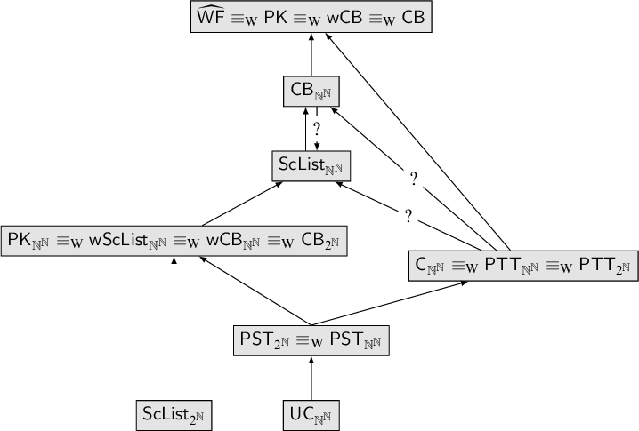
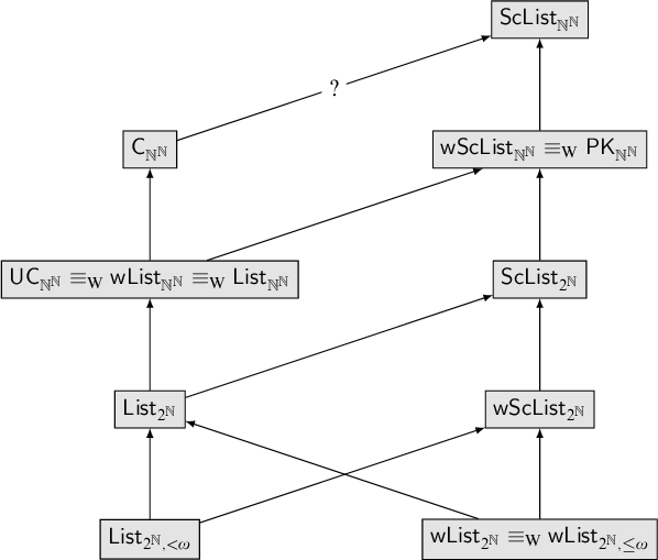
Figures 1 and 2 summarize some of our results. The precise definitions of the various functions are given in due time.
Some multi-valued functions studied in this paper. The arrows represent Weihrauch reducibility in the direction of the arrow. The question marks indicate that the existence of a reduction is still open. If a function cannot be reached from another one following a path of arrows, we know that there is no reduction between the two functions.

Multi-valued functions related to listing problems in the Weihrauch lattice. The arrows have the same meaning of Figure 1.

The paper is organized as follows. In Section 2, we give the necessary preliminaries: namely, in the first part, we provide definitions and notations about trees together with some useful lemmas, while in the second part we deal with represented spaces and Weihrauch reducibility. In Section 3, we study multi-valued functions related to the perfect set and perfect tree theorem in Baire and Cantor space, while in Section 4 we consider problems related to the Cantor–Bendixson theorem in the same setting. In Section 5, we study the problems considered in Sections 3 and 4 for arbitrary computable metric spaces, while Section 6 lists some open problems that remain to be solved.
2 Background
2.1 Sequences and trees
Let
 $\mathbb {N}^n$
denote the set of finite sequences of natural numbers of length n, where the length is denoted by
 $\left |{\cdot }\right |$
. If
 $n=0$
,
 $\mathbb {N}^0=\{\langle \rangle \}$
, where
 $\langle \rangle $
is the empty sequence: in general, given
 $i_0,\dots ,i_{n-1} \in \mathbb {N}$
, we denote by
 $\langle i_0,\dots ,i_{n-1} \rangle $
the finite sequence in
 $\mathbb {N}^n$
having digits
 $i_0,\dots ,i_{n-1}$
. The set of all finite sequences of natural numbers is denoted by
 $\mathbb {N}^{<\mathbb {N}}$
, while we write
 $2^{<\mathbb {N}}$
for the set of all finite sequences of
 $0$
and
 $1$
. For
 $\sigma \in \mathbb {N}^{<\mathbb {N}}$
and
 $m\leq \left |{\sigma }\right |$
, let
 $\sigma [m]:=\langle \sigma (0),\dots ,\sigma (m-1) \rangle $
. Given
 $\sigma , \tau \in \mathbb {N}^{<\mathbb {N}}$
, we use
 $\sigma \sqsubseteq \tau $
to say that
 $\sigma $
is an initial segment of
 $\tau $
(equivalently,
 $\tau $
an extension of
 $\sigma $
), i.e.,
 $\sigma =\tau [m]$
for some
 $m \leq \left |{\sigma }\right |$
. We use the symbol
 $\sqsubset $
in case
 $\sigma \sqsubseteq \tau $
and
 $\left |{\sigma }\right |<\left |{\tau }\right |$
, and in case
 $\sigma \not \sqsubseteq \tau $
and
 $\tau \not \sqsubseteq \sigma $
we say that
 $\sigma $
and
 $\tau $
are incomparable (
 $\sigma ~|~ \tau $
).
The concatenation of two finite sequences
 $\sigma ,\tau $
is denoted by
 $\sigma ^\smallfrown \tau $
, but often we just write
 $\sigma \tau $
. The same symbol is also used for the concatenation of a finite and an infinite sequence. For
 $n,k \in \mathbb {N}$
, we denote by
 $n^k$
the sequence made of k many n’s: in case
 $k=1$
we just write n and we use
 $n^{\mathbb {N}}$
to denote the infinite sequence with constant value n. For
 $\sigma \in \mathbb {N}^{<\mathbb {N}}$
and
 $p \in \mathbb {N}^{\mathbb {N}}$
we denote by
 $\sigma ^-$
and
 $p^-$
the result of deleting the first digit of the sequence.
Remark 2.1. We fix a bijection between
 $\mathbb {N}^{<\mathbb {N}}$
and
 $\mathbb {N}$
: to avoid too much notation, we do not introduce a specific symbol for this bijection, but we identify a sequence with the number representing it: it should be clear from the context whether we are referring to a finite sequence or to the number representing it. We need the bijection to enjoy all the usual properties such as
 $\sigma \mapsto \left |{\sigma }\right |$
being computable: moreover, we require that if
 $\sigma \sqsubset \tau $
then
 $\sigma <\tau $
.
A tree T is a nonempty subset of
 $\mathbb {N}^{<\mathbb {N}}$
closed under initial segments. In case the tree T is a subset of
 $2^{<\mathbb {N}}$
, we call T a binary tree. We say that
 $f \in \mathbb {N}^{\mathbb {N}}$
is a path through T if for all
 $n \in \mathbb {N}$
,
 $f[n]\in T$
where, as for finite sequences,
 $f[n]=\langle f(0),\dots ,f(n-1) \rangle $
. We denote by
 $\left [{T}\right ]$
the body of T, that is the set of paths through T. We say that a tree T is ill-founded iff there exists at least one path in
 $\left [{T}\right ]$
and well-founded otherwise. Given
 $\sigma \in T$
we define the tree of extensions of
 $\sigma $
in T as
 $T_{\sigma }:=\{\tau :\tau \sqsubseteq \sigma \lor \tau \sqsupseteq \sigma \}$
. Notice that
 $T_\sigma $
is ill-founded iff there exists a path through T that extends
 $\sigma $
. We say that T is perfect if every element of T has (at least) two incompatible extensions in T, that is,
 $(\forall \sigma \in T)(\exists \tau ,\tau ' \in T)(\sigma \sqsubset \tau \land \sigma \sqsubset \tau ' \land \tau ~|~ \tau ')$
. It is straightforward that the body of a nonempty perfect tree has uncountably many paths. Given a tree T, the largest perfect subtree S of T is called the perfect kernel of T while
 $\left [{T}\right ] \setminus \left [{S}\right ] \subseteq \mathbb {N}^{\mathbb {N}}$
is called the scattered part of T. We call T pruned if every
 $\sigma \in T$
has a proper extension. Notice that every perfect tree is pruned. Moreover, if
 $\left [{T}\right ]$
is perfect and T is pruned then T is a perfect tree.
Remark 2.2. It is useful to notice that, for a binary tree T, if
 $\left |{\left [{T}\right ]}\right |>\aleph _0$
then there must be uncountably many paths with infinitely many ones. In other words, it can’t be the case that all the paths in
 $\left [{T}\right ]$
are eventually zero paths, as it is straightforward to notice that they are only countably many.
Given trees T and S, we define the disjoint union of T and S as
 $T\sqcup S=\{\langle \rangle \} \cup \{\langle 0 \rangle \tau : \tau \in T \} \cup \{\langle 1 \rangle \tau : \tau \in S \}$
. Of course, this is still a tree and it has the property that
 $T\sqcup S$
is ill-founded iff at least one of T and S is ill-founded. The construction can be easily generalized to countably many trees letting
 $\bigsqcup _{{i\in \mathbb {N}}}{T^i}:=\{\langle \rangle \} \cup \{\langle i \rangle \tau :\tau \in T^i \land i \in \mathbb {N}\}$
and we still have that
 $\bigsqcup _{{i\in \mathbb {N}}}{T^i}$
is ill-founded iff there exists i such that
 $T^i$
is ill-founded. We also define the binary disjoint union as

Remark 2.3. Notice that if all the
 $T^i$
’s are binary trees, also
 is and, regardless the ill-foundedness/well-foundedness of the
 $T^i$
’s,
 . Moreover
 . In particular,
 iff there exists an
 $i \in \mathbb {N}$
such that
 $T^i$
is ill-founded.
We now turn our attention to another operation on trees, namely interleaving. Given
 $\sigma ,\tau \in \mathbb {N}^{n}$
, we define
 $\sigma *\tau :=\langle \sigma (0),\tau (0),\dots ,\sigma (n-1),\tau (n-1) \rangle $
. The same definition applies to infinite sequences. Then given trees T and S, the interleaving between T and S is
 $T*S:=\{ \sigma *\tau : \left |{\sigma }\right |=\left |{\tau }\right | \land \sigma \in T \land \tau \in S\}$
. Clearly,
 $T*S$
is a tree and it is ill-founded iff both T and S are ill-founded. This construction can be generalized to countably many trees in a straightforward way and we use a notation such as
 $\underset {i \in \mathbb {N}}{*}T^i$
.
We often use the interleaving
 $\mathsf {Expl}(T):= T*2^{<\mathbb {N}}$
, which we call the explosion of T.
Sometimes it is useful to be able to “translate” back and forth between sequences of natural numbers and binary sequences.
Definition 2.4. We define:
-
•
 $\rho _{2^{\mathbb {N}}}\colon \mathbb {N}^{<\mathbb {N}} \rightarrow 2^{<\mathbb {N}}$
by
$\rho _{2^{\mathbb {N}}}(\sigma ):=0^{\sigma (0)}10^{\sigma (1)}1\dots 10^{\left |{\sigma }\right |-1}1$
; in particular,
$\rho _{2^{\mathbb {N}}}(\langle \rangle ):=\langle \rangle $
;
-
•
$\rho _{\mathbb {N}^{\mathbb {N}}}\colon 2^{<\mathbb {N}}\rightarrow \mathbb {N}^{<\mathbb {N}}$
by
$$\begin{align*}\kern-6pt\rho_{\mathbb{N}^{\mathbb{N}}}(\tau):= \begin{cases} \rho_{2^{\mathbb{N}}}({\tau[n_\tau+1]})^{-1} &\text{if } (\exists i)(\tau(i)=1) \text{ where } n_\tau:=\max \{i:\tau(i)=1\}; \\ \langle \rangle & \text{if } (\forall i)(\tau(i)=0). \end{cases}\end{align*}$$


The two functions defined above have the following properties:
-
•
$\rho _{2^{\mathbb {N}}}$
is injective; -
•
$\rho _{\mathbb {N}^{\mathbb {N}}}(\rho _{2^{\mathbb {N}}}(\sigma ))=\sigma $
; -
•
$\sigma \sqsubset \sigma '$
iff
$\rho _{2^{\mathbb {N}}}(\sigma ) \sqsubset \rho _{2^{\mathbb {N}}}(\sigma ')$
; -
• if
$\tau \sqsubset \tau '$
then
$\rho _{\mathbb {N}^{\mathbb {N}}}(\tau ) \sqsubseteq \rho _{\mathbb {N}^{\mathbb {N}}}(\tau ')$
.


We are now able to “translate” back and forth between trees on
 $\mathbb {N}$
and binary trees. We use the same symbols
 $\rho _{2^{\mathbb {N}}}$
and
 $\rho _{\mathbb {N}^{\mathbb {N}}}$
as the context explains which function we are using.
Definition 2.5. Let
 $T\subseteq 2^{<\mathbb {N}}$
and
 $S\subseteq \mathbb {N}^{<\mathbb {N}}$
be trees. We define:
-
•
$\rho _{\mathbb {N}^{\mathbb {N}}}(T):=\{\sigma \in \mathbb {N}^{<\mathbb {N}}: \rho _{2^{\mathbb {N}}}(\sigma ) \in T\}$
; -
•
$\rho _{2^{\mathbb {N}}}(S):=\{\tau \in 2^{<\mathbb {N}}:\rho _{\mathbb {N}^{\mathbb {N}}}(\tau )\in S\}$
.


Remark 2.6. Notice that, since
 $\rho _{2^{\mathbb {N}}}(\sigma 0^n)=\rho _{2^{\mathbb {N}}}(\sigma )$
for every n, if
 $\sigma \in \rho _{\mathbb {N}^{\mathbb {N}}}(T)$
then
 $\sigma 0^{\mathbb {N}} {\kern-1pt}\in{\kern-1pt} \left [{\rho _{\mathbb {N}^{\mathbb {N}}}(T)}{\kern-1pt}\right ]$
. It is straightforward to check that
 $\rho _{\mathbb {N}^{\mathbb {N}}}(T){\kern-1pt}={\kern-1pt}\{\rho _{\mathbb {N}^{\mathbb {N}}}(\tau ) \in \mathbb {N}^{<\mathbb {N}}: \tau {\kern-1pt}\in{\kern-1pt} T\}$
. On the other hand, for most trees,
 $S\subseteq \mathbb {N}^{<\mathbb {N}}$
,
 $\rho _{2^{\mathbb {N}}}(S) \neq \{\rho _{2^{\mathbb {N}}}(\tau ) \in 2^{<\mathbb {N}}: \tau \in S\}$
as the latter is not even a tree.
The back and forth translations between sequences in
 $\mathbb {N}^{\mathbb {N}}$
and
 $2^{\mathbb {N}}$
are also denoted by the same function symbols used for finite sequences and for trees: again the context clarifies which one we are using.
Definition 2.7.
-
•
$\rho _{2^{\mathbb {N}}}\colon \mathbb {N}^{\mathbb {N}} {\kern-1pt}\rightarrow{\kern-1pt} 2^{\mathbb {N}}$
is defined by
$\rho _{2^{\mathbb {N}}}(p):=\underset {n \in \mathbb {N}}{\bigcup }\rho _{2^{\mathbb {N}}}(p[n])=0^{p(0)}10^{p(1)}\dots 10^{p(n)}1\dots $
; -
•
${\rho _{\mathbb {N}^{\mathbb {N}}}} :\subseteq {2^{\mathbb {N}}}\rightarrow {\mathbb {N}^{\mathbb {N}}}$
has domain
$\{q:(\exists ^\infty i)(q(i)=1)\}$
and is defined by
$\rho _{\mathbb {N}^{\mathbb {N}}}(q):=\underset {n \in \mathbb {N}}{\bigcup }\rho _{\mathbb {N}^{\mathbb {N}}}(q[n])$
.


In both definitions, the union makes sense because the finite sequences are comparable.
Notice that all the functions
 $\rho _{\mathbb {N}^{\mathbb {N}}}$
and
 $\rho _{2^{\mathbb {N}}}$
we defined are computable. For the functions on finite sequences, this means usual Turing computability. For the functions on trees and infinite sequences computability is to be intended in the sense of Section 2.2.
Lemma 2.8. The following lemma summarizes the fundamental properties of
 $\rho _{2^{\mathbb {N}}}$
and
 $\rho _{\mathbb {N}^{\mathbb {N}}}$
for infinite sequences and trees.
-
1. The range of
$\rho _{2^{\mathbb {N}}}$
is
$\{q \in 2^{\mathbb {N}}:(\exists ^\infty i)(q(i)=1)\}$
; -
2.
$\rho _{\mathbb {N}^{\mathbb {N}}}(\rho _{2^{\mathbb {N}}}(p))=p$
for every
$p \in \mathbb {N}^{\mathbb {N}}$
. -
3.
$\rho _{2^{\mathbb {N}}}(\rho _{\mathbb {N}^{\mathbb {N}}}(q))=q$
for every
$q \in \operatorname {dom}(\rho _{\mathbb {N}^{\mathbb {N}}})$
. -
4. If
$S\subseteq \mathbb {N}^{<\mathbb {N}}$
,
$p \in \left [{S}\right ] \iff \rho _{2^{\mathbb {N}}}(p)\in \left [{\rho _{2^{\mathbb {N}}}(S)}\right ]$
and hence
$\left [{\rho _{2^{\mathbb {N}}}(S)}\right ]\subseteq \{\rho _{2^{\mathbb {N}}}(p): p \in \left [{S}\right ]\}\cup \{q:(\forall ^{\infty } i)(q(i)=0)\}$
so that
$\left |{\left [{\rho _{2^{\mathbb {N}}}(S)}\right ]}\right |\leq \aleph _0 \iff \left |{\left [{S}\right ]}\right | \leq \aleph _0$
. -
5. If
$T\subseteq 2^{<\mathbb {N}}$
and
$q \in \operatorname {dom}(\rho _{\mathbb {N}^{\mathbb {N}}})$
we have that
$q \in \left [{T}\right ] \iff \rho _{\mathbb {N}^{\mathbb {N}}}(q) \in \left [{\rho _{\mathbb {N}^{\mathbb {N}}}(T)}\right ]$
. -
6. If
$T\subseteq 2^{<\mathbb {N}}$
and
$p \in \mathbb {N}^{\mathbb {N}}$
then
$p \in \left [{\rho _{\mathbb {N}^{\mathbb {N}}}(T)}\right ] \iff \rho _{2^{\mathbb {N}}}(p) \in \left [{T}\right ]$
.


Proof. The proofs are straightforward from the definitions above.
Lemma 2.9. If T is a binary tree such that
 $\left [{T}\right ]$
is perfect then
 $\left [{\rho _{\mathbb {N}^{\mathbb {N}}}(T)}\right ]$
is perfect as well. Furthermore, if T is a perfect tree then
 $\rho _{\mathbb {N}^{\mathbb {N}}}(T)$
is a perfect tree as well.
Proof. Let T be a binary tree such that
 $\left [{T}\right ]$
is perfect. We show that no
 $f \in \left [{\rho _{\mathbb {N}^{\mathbb {N}}}(T)}\right ]$
is isolated, i.e.,
 $(\forall n)(\exists g \in \left [{\rho _{\mathbb {N}^{\mathbb {N}}}(T)}\right ])(f[n] \sqsubset g \land f \neq g)$
. Fix n: by Theorem 2.8(6) we get that
 $\rho _{2^{\mathbb {N}}}(f) \in \left [{T}\right ]$
and, in particular,
 $\sigma := \rho _{2^{\mathbb {N}}}(f[n]) \in T$
. Since
 $\left [{T}\right ]$
is perfect, by Theorem 2.2, there exists
 $h \in \left [{T}\right ]$
with infinitely many ones such that
 $\sigma \sqsubset h$
and
 $\rho _{2^{\mathbb {N}}}(f) \neq h$
. By Theorem 2.8(5)
 $\rho _{\mathbb {N}^{\mathbb {N}}}(h) \in \left [{\rho _{\mathbb {N}^{\mathbb {N}}}(T)}\right ]$
and letting
 $g:= \rho _{\mathbb {N}^{\mathbb {N}}}(h)$
, we reach the conclusion.
In case T is a perfect tree, it suffices to show that
 $\rho _{\mathbb {N}^{\mathbb {N}}}(T)$
is pruned. Suppose there exists
 $\sigma \in \rho _{\mathbb {N}^{\mathbb {N}}}(T)$
with no extensions in
 $\rho _{\mathbb {N}^{\mathbb {N}}}(T)$
. Then
 $\tau := \rho _{2^{\mathbb {N}}}(\sigma )$
belongs to T and the only path in T extending
 $\tau $
is of the form
 $\tau 0^{\mathbb {N}}$
, contradicting the perfectness of T.
Notice that if
 $S\subseteq \mathbb {N}^{<\mathbb {N}}$
is a perfect tree it may be the case that
 $\left [{\rho _{2^{\mathbb {N}}}(S)}\right ]$
is not perfect, e.g., let
 $S=\{\sigma \in \mathbb {N}^{<\mathbb {N}}:\sigma (0)=0\}$
and notice that
 $0^{\mathbb {N}}$
is isolated in
 $\left [{\rho _{2^{\mathbb {N}}}(S)}\right ]$
.
2.2 Represented spaces and Weihrauch reducibility
We give a brief introduction to computable analysis and the theory of represented spaces. We refer the reader to [Reference Brattka, Gherardi, Pauly, Brattka and Hertling8] and [Reference Weihrauch26] for more on these topics. In particular, we assume the notion of partial computable function from
 $\mathbb {N}^{\mathbb {N}}$
to
 $\mathbb {N}^{\mathbb {N}}$
, as formulated in the so-called TTE theory of computation. We denote by
 $\Phi _e$
the partial function computed by the Turing machine of index
 $e \in \mathbb {N}$
.
A represented space
 $\textbf {X}$
is a pair
 $(X,\delta _{X})$
where X is a set and
 ${{\delta _{X}}} :\subseteq {\mathbb {N}^{\mathbb {N}}}\rightarrow {X}$
is a (possibly partial) surjection. For each
 $x \in X$
we say that p is a
 $\delta _{X}$
-name for x if
 $\delta _{X}(p)=x$
.
A computational problem f between represented spaces
 $\textbf {X}$
and
 $\textbf {Y}$
is formalized as a partial multi-valued function
 ${{f}} :\subseteq {\textbf {X}} \rightrightarrows {\textbf {Y}}$
. A (possibly partial) function
 ${{F}} :\subseteq {\mathbb {N}^{\mathbb {N}}}\rightarrow {\mathbb {N}^{\mathbb {N}}}$
is a realizer for
 ${{f}} :\subseteq {\textbf {X}} \rightrightarrows {\textbf {Y}}$
if for every
 $p \in \operatorname {dom}(f\circ \delta _X)$
,
 $\delta _Y(F(p)) \in f(\delta _X(p))$
. The notion of realizer allows us to transfer properties of functions on the Baire space (such as computability or continuity) to multi-valued functions defined on represented spaces in general. Whenever we say that a multi-valued function between represented spaces is computable we mean that it has a computable realizer.
We fix a computable enumeration
 $(q_i)_{i \in \mathbb {N}}$
of
 $\mathbb {Q}$
and we represent the space
 $\mathbb {R}$
by the so-called Cauchy representation
 $\delta _{\mathbb {R}}$
where
 $\operatorname {dom}(\delta _{\mathbb {R}}):=\{p \in \mathbb {N}^{\mathbb {N}}:(\forall j) (\forall i>j)(|q_{p(i)}-q_{p(j)}|<2^{-j})\}$
and
 $\delta _{\mathbb {R}}(p) := \lim q_{p(n)}$
.
We can now represent any computable metric space
 $\mathcal {X}=(X,d,\alpha )$
, that is a separable metric space
 $(X,d)$
and a dense sequence
 ${\alpha }:{\mathbb {N}}\rightarrow {X}$
such that
 ${d\circ (\alpha \times \alpha )}:{\mathbb {N}^2}\rightarrow {\mathbb {R}}$
is a computable double sequence of real numbers. The Cauchy representation
 ${{\delta _X}} :\subseteq {\mathbb {N}^{\mathbb {N}}}\rightarrow {X}$
of such a space has domain
 $\{p \in \mathbb {N}^{\mathbb {N}}:(\forall j)(\forall i>j) (d(\alpha (p(i)),\alpha (p(j)))<2^{-j})\}$
and is defined by
 $\delta _X(p)=\lim \alpha (p(n))$
. We always assume that computable metric spaces are represented by this representation. For convenience, we fix a computable enumeration
 $(B_i)_{i \in \mathbb {N}}$
of all basic open sets of
 $\mathcal {X}$
, where the ball
 $B_{\langle n,m \rangle }$
is centered in
 $\alpha (n)$
and has radius
 $q_m$
.
A computable Polish space is a computable metric space
 $\mathcal {X}=(X,d,\alpha )$
such that the metric d is complete.
Given a computable metric space
 $\mathcal {X}$
and
 $k>0$
, using the inductive definition of Borel sets, we can define the represented spaces
 $\boldsymbol {\Sigma }_k^0(\mathcal {X})$
,
 $\boldsymbol {\Pi }_k^0(\mathcal {X})$
and
 $\boldsymbol {\Delta }_k^0(\mathcal {X})$
: this shows that the Borel classes can be naturally considered as represented spaces.
Definition 2.10 [Reference Brattka2, Definition 3.1].
For any computable metric space
 $\mathcal {X}=(X,d,\alpha )$
and for any
 $k>0$
, we define the represented spaces
 $(\boldsymbol {\Sigma }_k^0(\mathcal {X}),\delta _{\boldsymbol {\Sigma }_k^0(\mathcal {X})})$
,
 $(\boldsymbol {\Pi }_k^0(\mathcal {X}),\delta _{\boldsymbol {\Pi }_k^0(\mathcal {X})})$
and
 $(\boldsymbol {\Delta }_k^0(\mathcal {X}),\delta _{\boldsymbol {\Delta }_k^0(\mathcal {X})})$
inductively as follows:
-
•
$\delta _{\boldsymbol {\Sigma }_1^0(\mathcal {X})}(p):=\underset {i \in \mathbb {N}}{\bigcup }B_{p(i)}$
; -
•
$\delta _{\boldsymbol {\Pi }_k^0(\mathcal {X})}:= X\setminus \delta _{\boldsymbol {\Sigma }_k^0(\mathcal {X})}(p)$
; -
•
$\delta _{\boldsymbol {\Sigma }_{k+1}^0(\mathcal {X})}(p_0*p_1*\dots ):=\underset {i \in \mathbb {N}}{\bigcup }\delta _{\boldsymbol {\Pi }_k^0(\mathcal {X})}(p_i)$
.


Notice that the representation of
 $\boldsymbol {\Pi }_1^0(\mathcal {X})$
is the standard negative representation of closed sets of
 $\mathcal {X}$
: as usual in the literature, we denote this represented space by
 $\mathcal {A}({\mathcal {X}})$
. We denote by
 $\Pi _1^0(\mathcal {X})$
the collection of closed sets of
 $\mathcal {X}$
having a computable name.
Let
 $\mathbf {Tr}$
and
 $\mathbf {Tr}_2$
be the represented spaces of trees on
 $\mathbb {N}$
numbers and binary trees, respectively: for both the representation map is the characteristic function and hence we identify
 $\mathbf {Tr}$
and
 $\mathbf {Tr}_2$
with closed subsets of
 $2^{\mathbb {N}}$
. The surjective function
 ${[\cdot ]}:{\mathbf {Tr}}\rightarrow {\mathcal {A}({\mathbb {N}^{\mathbb {N}}})}$
defined by
 $T\mapsto \left [{T}\right ]$
is computable with multi-valued computable inverse and the same holds for its restriction to
 $\mathbf {Tr}_2$
, which is onto
 $\mathcal {A}({2^{\mathbb {N}}})$
. This means that the negative representation of a closed subset C of
 $\mathbb {N}^{\mathbb {N}}$
(resp.
 $2^{\mathbb {N}}$
) is equivalent (in the sense of [Reference Weihrauch26, Definition 2.3.2]) to the one given by the characteristic function of a (resp. binary) tree T such that
 $\left [{T}\right ]=C$
. We refer to the latter representation as the tree representation.
We can represent the pointclass
 $\boldsymbol {\Sigma }_1^1(\mathcal {X})$
of analytic subsets of
 $\mathcal {X}$
by defining a name for S as a name for a closed set
 $C\subseteq \mathcal {X}\times \mathbb {N}^{\mathbb {N}}$
such that S is the projection on the first coordinate of C. Then, a name for a coanalytic set
 $R \in \boldsymbol {\Pi }_1^1(\mathcal {X})$
is just a name for its complement.
The next theorem summarizes some well-known results about the level at which some subsets of trees are in the Kleene arithmetical and analytical hierarchy (or lightface hierarchy), the effective counterpart of the Borel and projective hierarchy (or boldface hierarchy). Here, completeness is defined with respect to effective Wadge reducibility. These notions can be found, sometimes with different terminology, for example in [Reference Kechris14, Reference Moschovakis20].
Theorem 2.11. The following classification results hold:
-
(i) The set
$\mathcal {IF}:= \{T \in \mathbf {Tr} : T \text { is ill-founded}\}$
is
$\Sigma _1^1$
-complete, while
$\mathcal {WF}:= \{T \in \mathbf {Tr} : T \text { is well-founded}\}$
is
$\Pi _1^1$
-complete. In contrast,
$\mathcal {IF}_2:= \mathcal {IF} \cap \mathbf {Tr}_2$
is
$\Pi _1^0$
-complete and
$\mathcal {WF}_2:= \mathcal {WF} \cap \mathbf {Tr}_2$
is
$\Sigma _1^0$
-complete. -
(ii) The set
$\mathcal {T}^{>\aleph _0}:= \{T \in \mathbf {Tr}: \left |{\left [{T}\right ]}\right | > \aleph _0\}$
is
$\Sigma _1^1$
-complete, while
$\mathcal {T}^{\leq \aleph _0} := \{T \in \mathbf {Tr}: \left |{\left [{T}\right ]}\right | \leq \aleph _0\}$
is
$\Pi _1^1$
-complete. In this case,
$\mathcal {T}^{>\aleph _0}_2 := \mathcal {T}^{>\aleph _0} \cap \mathbf {Tr}_2$
is
$\Sigma _1^1$
-complete as well and
$\mathcal {T}^{\leq \aleph _0}_2 := \mathcal {T}^{\leq \aleph _0} \cap \mathbf {Tr}_2$
is also
$\Pi _1^1$
-complete. -
(iii) The set
$\mathcal {UB}:= \{T \in \mathbf {Tr} : \left |{\left [{T}\right ]}\right |=1\}$
is
$\Pi _1^1$
-complete. In contrast,
$\mathcal {UB}_2 := \mathcal {UB}\cap \mathbf {Tr}_2$
is
$\Pi _2^0$
-complete.




Proof. To show that
 $\mathcal {IF}$
is
 $\Sigma _1^1$
-complete see [Reference Kechris14, Theorem 27.1]: the theorem states the boldface case, but its proof works also in the lightface one. If
 $T\in \mathbf {Tr}_2$
, notice that, by König’s lemma,
 $T \in \mathcal {IF}_2$
iff
 $(\forall n)(\exists \tau \in 2^{n})(\tau \in T)$
; hence
 $\mathcal {IF}_2$
is
 $\Pi _1^0$
and completeness is straightforward. It follows immediately that
 $\mathcal {WF}$
is
 $\Pi _1^1$
-complete and
 $\mathcal {WF}_2$
is
 $\Sigma _1^0$
-complete.
To prove that
 $\mathcal {T}^{>\aleph _0}$
is
 $\Sigma _1^1$
-complete notice that, by the Cantor–Bendixson theorem for trees,
 $T \in \mathcal {T}^{>\aleph _0} $
iff
 $(\exists S \subseteq T)(S \text { is nonempty and perfect})$
: the latter is a
 $\Sigma _1^1$
formula and it remains to show that
 $\mathcal {T}^{>\aleph _0}$
is complete for
 $\Sigma _1^1$
sets. This is immediate as
 $T \in \mathcal {IF} \iff \mathsf {Expl}(T) \in \mathcal {T}^{>\aleph _0}$
. The proof for
 $\mathcal {T}^{>\aleph _0}_2$
is similar and it follows immediately that
 $\mathcal {T}^{\leq \aleph _0}$
and
 $\mathcal {T}^{\leq \aleph _0}_2$
are
 $\Pi _1^1$
-complete.
To prove that
 $\mathcal {UB}$
is
 $\Pi _1^1$
-complete notice that, by the effective perfect set theorem (see [Reference Moschovakis20, Theorem 4F.1]),
 $T \in \mathcal {UB}$
iff
 $$\begin{align*}(\exists p \in \mathsf{HYP}(\mathbb{N}^{\mathbb{N}}))(p \in \left[{T}\right]) \land (\forall \tau,\tau')(\tau ~|~ \tau' \implies T_\tau \in \mathcal{WF} \lor T_{\tau'} \in \mathcal{WF}),\end{align*}$$
where
 $\mathsf {HYP}(\mathbb {N}^{\mathbb {N}})$
is the set of hyperarithmetical elements in
 $\mathbb {N}^{\mathbb {N}}$
. Notice that the formula is
 $\Pi _1^1$
: indeed, the second conjunct is clearly
 $\Pi _1^1$
and by Kleene’s quantification theorem (see [Reference Moschovakis20, Theorem 4D.3]), the first conjunct is
 $\Pi _1^1$
as well. It remains to show that
 $\mathcal {UB}$
is complete for
 $\Pi _1^1$
sets. To do so, it suffices to notice that
 $T \in \mathcal {WF}$
iff
 $S \in \mathcal {UB}$
, where
 $S:= \{0^n:n \in \mathbb {N}\} \sqcup T$
(indeed,
 $\left [{S}\right ]=\{0^{\mathbb {N}}\} \cup \{1p:p \in \left [{T}\right ]\}$
). If
 $T \in \mathbf {Tr}_2$
, notice that
 $T \in \mathcal {UB}_2$
iff
 $$\begin{align*}T \in \mathcal{IF}_2 \land (\forall \tau,\tau')(\tau ~|~ \tau' \implies T_\tau \in \mathcal{WF}_2 \lor T_{\tau'} \in \mathcal{WF}_2).\end{align*}$$
The formula is clearly
 $\Pi _2^0$
and proving completeness is straightforward.
To compare the uniform computational content of different problems, we use the framework of Weihrauch reducibility. We say that a problem f is Weihrauch reducible to a problem g, written
 $f \le _{\mathrm {W}} g$
, if there are computable maps
 ${{\Phi ,\Psi }} :\subseteq {\mathbb {N}^{\mathbb {N}}}\rightarrow {\mathbb {N}^{\mathbb {N}}}$
such that if p is a name for some
 $x \in \operatorname {dom}(f)$
, then:
-
(i)
$\Phi (p)$
is a name for some
$y \in \operatorname {dom}(g)$
; -
(ii) for every name q for some element of
$g(y)$
,
$\Psi (p*q)$
is a name for some element of
$f(x)$
.


Informally, if
 $f\le _{\mathrm {W}} g$
we are claiming the existence of a procedure for solving f which is computable modulo a single invocation of g as an oracle (in other words, this procedure transforms realizers for g into realizers for f). In case
 $\Phi $
is as above and
 $\Psi $
is not allowed to use p in its computation, we say that f is strongly Weihrauch reducible to a problem g, written
 $f \le _{\mathrm {sW}} g$
.
Weihrauch reducibility and strong Weihrauch reducibility are reflexive and transitive hence they induce the equivalence relations
 $\equiv _{\mathrm {W}}$
and
 $\equiv _{\mathrm {sW}}$
: that is
 $f\equiv _{\mathrm {W}} g$
iff
 $f \le _{\mathrm {W}} g$
and
 $g\le _{\mathrm {W}} f$
(similarly for
 $\le _{\mathrm {sW}}$
). The
 $\equiv _{\mathrm {W}}$
-equivalence classes are called Weihrauch degrees (similarly the
 $\equiv _{\mathrm {sW}}$
-equivalence classes are called strong Weihrauch degrees). Both the Weihrauch degrees and the strong Weihrauch degrees form lattices (see [Reference Brattka, Gherardi, Pauly, Brattka and Hertling8, Theorems 3.9 and 3.10]).
There are several natural operations on problems which also lift to the
 $\equiv _{\mathrm {W}}$
-degrees and the
 $\equiv _{\mathrm {sW}}$
-degrees: we mention below the ones we need.
-
• The parallel product
$f \times g$
is defined by
$(f \times g)(x,y) := f(x) \times g(y)$
. -
• The finite parallelization is defined as
$f^*((x_i)_{i<n}):=\{(y_i)_{i<n}:(\forall i<n)(y_i \in f(x_i))\}$
. -
• The infinite parallelization is defined as
$\widehat {f}((x_i)_{i \in \mathbb {N}}):=\{(y_i)_{i \in \mathbb {N}}:(\forall i)(y_i \in f(x_i)\}$
.


Informally, the three operators defined above capture, respectively, the idea of using f and g in parallel, using f a finite (but given in the input) number of times in parallel, and using f countably many times in parallel.
The following definition, with a slightly different notation, was recently given by Soldà and the third author.
Definition 2.12 [Reference Soldà and Valenti25].
For every
 ${{f}} :\subseteq {\mathbf {X}} \rightrightarrows {\mathbf {Y}}$
, define the finite unbounded parallelization
 ${{f^{u*}}} :\subseteq {\mathbb {N} \times \mathbb {N}^{\mathbb {N}} \times \mathbf {X}} \rightrightarrows {(\mathbb {N}^{\mathbb {N}})^{<\mathbb {N}}}$
as follows:
-
• instances are triples
$(e,w,(x_n)_{n \in \mathbb {N}})$
such that
$(x_n)_{n \in \mathbb {N}} \in \operatorname {dom}(\widehat {f})$
and for each sequence
$(q_n)_{n \in \mathbb {N}}$
with
$\delta _{Y}(q_n) \in f(x_n)$
, there is a
$k\in \mathbb {N}$
such that
$\Phi _e(w,q_0*\dots * q_{k-1})(0)\downarrow $
in k steps; -
• a solution for
$(e,w,(x_n)_{n \in \mathbb {N}})$
is a finite sequence
$(q_n)_{n<k}$
such that for every
$n <k$
,
$\delta _{Y}(q_n)\in f(x_n)$
and
$\Phi _e(w,q_0*\dots * q_{k-1})(0)\downarrow $
in k steps.


Informally,
 $f^{u*}$
takes an input a Turing functional with a parameter and an input for
 $\widehat {f}$
and outputs “sufficiently many” names for solutions where “sufficiently many” is determined by the convergence of the Turing functional in input.
We call f a cylinder if
 $f \equiv _{\mathrm {sW}} f \times \operatorname {id}$
. If f is a cylinder, then
 $g \le _{\mathrm {W}} f$
iff
 $g \le _{\mathrm {sW}} f$
[Reference Brattka and Gherardi5, Corollary 3.6]. This is useful for establishing nonreductions because, if f is a cylinder, then it suffices to diagonalize against all strong Weihrauch reductions from g to f in order to show that
 $g \not \le _{\mathrm {W}} f$
. Cylinders are also useful when working with compositional products (discussed below). Observe that for every problem f,
 $f \times \operatorname {id}$
is a cylinder which is Weihrauch equivalent to f.
The compositional product
 $f * g$
captures the idea of what can be achieved by first applying g, possibly followed by some computation, and then applying f. Formally,
 $f*g$
is any function satisfying
 $$\begin{align*}f * g \equiv_{\mathrm{W}} \max_{\le_{\mathrm{W}}} \{f_1 \circ g_1 {}\,:\,{} f_1 \le_{\mathrm{W}} f \land g_1 \le_{\mathrm{W}} g\}. \end{align*}$$
This operator was first introduced in [Reference Brattka, Gherardi and Marcone7], and proven to be well-defined in [Reference Brattka and Pauly10]. For each problem f, we denote by
 $f^{[n]}$
the n-fold iteration of the compositional product of f with itself, i.e.,
 $f^{[1]} = f$
,
 $f^{[2]} = f * f$
, and so on.
Many (non) reductions in this paper follow from the characterization of the first-order part
 ${}^1{f}$
and the deterministic part
 $\mathsf {Det}(f)$
of a problem f. The first was introduced in [Reference Dzhafarov, Solomon and Yokoyama11] and extensively studied in [Reference Soldà and Valenti25], and the second one was defined in [Reference Le Goh, Pauly and Valenti18].
We say that a computational problem f is first-order if its codomain is
 $\mathbb {N}$
. As we need only the following characterization of
 ${}^1{f}$
, we omit the technical definition (see e.g., [Reference Le Goh, Pauly and Valenti18, Definition 2.2]).
Theorem 2.13 [Reference Dzhafarov, Solomon and Yokoyama11].
For every problem f,
 ${}^1{f} \equiv _{\mathrm {W}} \max _{\le _{\mathrm {W}}}\{ g{}\,:\,{} g \text { is first-order and} g \le _{\mathrm {W}} f\}$
.
The following theorem relates the first-order part with the unbounded finite parallelization.
Theorem 2.14 [Reference Soldà and Valenti25, Theorem 5.7].
For every first-order f,
 ${}^1{(\widehat {f}) }\equiv _{\mathrm {W}} f^{u*}$
.
Similarly, we only need the following characterization of
 $\mathsf {Det}(f)$
and we omit the formal definition (see [Reference Le Goh, Pauly and Valenti18, Definition 3.1]).
Theorem 2.15 [Reference Le Goh, Pauly and Valenti18, Theorem 3.2].
For every problem f,
 $$\begin{align*}\mathsf{Det}(f) \equiv_{\mathrm{W}} \max_{\le_{\mathrm{W}}}\{g: {{g}} :\subseteq {X}\rightarrow {\mathbb{N}^{\mathbb{N}}} \land g \le_{\mathrm{W}} f\}.\end{align*}$$
Hence,
 $\mathsf {Det}(f)$
is the strongest single-valued function which Weihrauch reduces to f.
Other useful operations on problems do not lift to Weihrauch degrees (i.e., applying the operation to equivalent problems does not always produce equivalent problems).
The first such operation is the jump. First, we define the jump of a represented space
 $\mathbf {X}=(X,\delta _{X})$
. This is
 $\mathbf {X}'=(X,\delta _{X}')$
where
 $\delta _{X}'$
takes in input a sequence of elements of
 $\mathbb {N}^{\mathbb {N}}$
converging to some
 $p \in \operatorname {dom}(\delta _X)$
and returns
 $\delta _{X}(p)$
. Then for a problem
 ${{f}} :\subseteq {\textbf {X}} \rightrightarrows {\textbf {Y}}$
its jump
 $ {{f'}} :\subseteq {\textbf {X}'} \rightrightarrows {\textbf {Y}}$
is defined as
 $f'(x) := f(x)$
. In other words,
 $f'$
is the following task: given a sequence that converges to a name for an instance of f, produces a solution for that instance. The jump lifts to strong Weihrauch degrees but not to Weihrauch degrees (see [Reference Brattka, Gherardi and Marcone7, Section 5]). We use
 $f^{(n)}$
to denote the n-th iterate of the jump applied to f. Let
 $ {{\mathsf {lim}}} :\subseteq {(\mathbb {N}^{\mathbb {N}})^{\mathbb {N}}}\rightarrow {\mathbb {N}^{\mathbb {N}}}, \ (p_n)_{n \in \mathbb {N}}\mapsto \lim p_n$
be the single-valued function whose domain consists of all converging sequences in
 $\mathbb {N}^{\mathbb {N}}$
: we have
 $f^{(n)}\le _{\mathrm {W}} f* \mathsf {lim}^{[n]}$
, but the converse reduction does not hold in general.
We now introduce the totalization of a problem and the completion of a problem. These two operators are different ways of making a partial multi-valued function total; neither of them lifts to Weihrauch degrees. Given a partial multi-valued function
 ${{f}} :\subseteq {\mathbf {X}} \rightrightarrows {\mathbf {Y}}$
the totalization of f is the total multi-valued function
 $\mathsf {T}f$
defined as
 $$\begin{align*}\mathsf{T}f(x):=\begin{cases} f(x) & \text{ if } x \in \operatorname{dom}(f),\\ Y & \text{otherwise.} \end{cases} \end{align*}$$
For more details on the totalization we refer the reader to [Reference Brattka and Gherardi6].
To define the completion of a problem f we need to first introduce the completion of a represented space. We adopt the following notation: given
 $p \in \mathbb {N}^{\mathbb {N}}$
we define
 $\hat {p}_n$
to be
 $\langle \rangle $
if
 $p(n)=0$
,
 $\langle p(n)-1 \rangle $
otherwise; then
 $p-1$
is the concatenation of all the
 $\hat {p}_n$
’s. For a represented space
 $\mathbf {X}=(X, \delta _X)$
we define its completion as
 $\overline {\mathbf {X}}=(\overline {X}, \delta _{\overline {X}})$
where
 $\overline {X}=X\cup \{\bot \}$
with
 $\bot \notin X$
and
 ${\delta _{\overline {X}}}:{\mathbb {N}^{\mathbb {N}}}\rightarrow {\overline {X}}$
is the total function defined by
 $$\begin{align*}\delta_{\overline{X}}(p):=\begin{cases} \delta_X(p-1)& \text{if } p-1 \in \operatorname{dom}(\delta_X)\\ \bot &\text{otherwise.} \end{cases} \end{align*}$$
Let
 ${{f}} :\subseteq {\mathbf {X}} \rightrightarrows {\mathbf {Y}}$
be a multi-valued function. We define the completion of f as the total multi-valued function
 ${\overline {f}}: {\overline {\mathbf {X}}}\rightrightarrows {\overline {\mathbf {Y}}}$
such that
 $$\begin{align*}\overline{f}(x)= \begin{cases} f(x) & \text{ if } x \in \operatorname{dom}(f),\\ \overline{Y} & \text{ otherwise}. \end{cases} \end{align*}$$
We now introduce some major benchmarks in the Weihrauch lattice.
The well-known problem
 ${ \mathsf {LPO} }:{2^{\mathbb {N}}}\rightarrow {\{0,1\}}$
is defined as
 $ \mathsf {LPO} (p)=1$
iff
 $(\forall n)(p(n)=0)$
. It is convenient to think of
 $ \mathsf {LPO} $
as the function answering yes or no to questions which are
 $\Pi _1^{0}$
or
 $\Sigma _1^{0}$
in the input. Similarly,
 $ \mathsf {LPO} ^{(n)}$
can be seen as the function answering yes or no to questions which are
 $\Pi _{n+1}^0$
or
 $\Sigma _{n+1}^0$
in the input. It is well-known that
 $\mathsf {lim} \equiv _{\mathrm {sW}} \widehat { \mathsf {LPO} }$
. Moreover, using [Reference Brattka, Gherardi and Marcone7, Section 5], we obtain that for every n,
 $\mathsf {lim}^{(n)} \equiv _{\mathrm {sW}} \widehat { \mathsf {LPO} ^{(n)}}$
.
We define also
 ${\mathsf {WF}}:{\mathbf {Tr}}\rightarrow {\{0,1\}}$
as
 $\mathsf {WF}(T)=1$
iff
 $T \in \mathcal {WF}$
. Analogously to
 $ \mathsf {LPO} $
, we can think of
 $\mathsf {WF}$
as the problem answering yes or no to questions which are
 $\Pi _1^{1}$
or
 $\Sigma _1^{1}$
in the input. In the literature,
 $\mathsf {WF}$
was introduced under different names: the same notation appears in [Reference Hirst13, Reference Soldà and Valenti25], while [Reference Brattka and Gherardi6] uses
 $\mathsf {WFT}$
and [Reference Kihara, Marcone and Pauly15, Reference Marcone and Valenti19] use
 $\chi _{\Pi _1^1}$
.
We now move our attention to choice problems, which have emerged as very significant milestones in the Weihrauch lattice. For a computable metric space
 $\mathcal {X}$
and a pointclass
 $\boldsymbol {\Gamma }$
as the ones in Theorem 2.10, let
 ${{{\boldsymbol {\Gamma }}\text {-}\mathsf {C}^{\vphantom {g}\mathsf {}}_{{\mathcal {X}}} }} :\subseteq {\boldsymbol {\Gamma }(\mathcal {X})} \rightrightarrows {\mathcal {X}}$
be the problem that given in input a nonempty set
 $A \in \boldsymbol {\Gamma }(\mathcal {X})$
outputs a member of A. When
 $\boldsymbol {\Gamma }=\boldsymbol {\Pi }_1^0$
we just write
 $\mathsf {C}^{\mathsf {\vphantom {g}}}_{{\mathcal {X}}} $
. The same problem with domain restricted to singletons is denoted by
 $ {\boldsymbol {\Gamma }}\text {-}\mathsf {UC}^{\vphantom {g}\mathsf {}}_{{\mathcal {X}}} $
. It is well-known that for every
 $n>0$
,
 $({\boldsymbol {\Pi }_n^0}\text {-}\mathsf {C}^{\vphantom {g}\mathsf {}}_{{\mathbb {N}}} )'\equiv _{\mathrm {W}} {\boldsymbol {\Pi }_{n+1}^0}\text {-}\mathsf {C}^{\vphantom {g}\mathsf {}}_{{\mathbb {N}}} $
.
Using the tree representation of closed sets,
 $\mathsf {C}_{\mathbb {N}^{\mathbb {N}}}$
can be formulated as the problem of computing a path through some
 $T \in \mathcal {IF}$
;
 $\mathsf {UC}_{\mathbb {N}^{\mathbb {N}}}$
is the same problem with domain restricted to
 $\mathcal {UB}$
. Notice that both problems are closed under compositional product by [Reference Brattka, de Brecht and Pauly3, Theorem 7.3]. As noticed in [Reference Kihara, Marcone and Pauly15] and mentioned in the introduction,
 $\mathsf {C}_{\mathbb {N}^{\mathbb {N}}}$
and
 $\mathsf {UC}_{\mathbb {N}^{\mathbb {N}}}$
are among the problems that correspond to
 $\mathsf {ATR}_0$
. We need the following proposition.
Proposition 2.16.
 $\widehat { {\boldsymbol {\Pi }_1^1}\text {-}\mathsf {UC}^{\vphantom {g}\mathsf {}}_{{\mathbb {N}}} } \equiv _{\mathrm {W}} \widehat { {\boldsymbol {\Pi }_1^1}\text {-}\mathsf {C}^{\vphantom {g}\mathsf {}}_{{\mathbb {N}}} }\equiv _{\mathrm {W}}\mathsf {UC}_{\mathbb {N}^{\mathbb {N}}}<_{\mathrm {W}} \widehat {{\boldsymbol {\Sigma }_1^1}\text {-}\mathsf {C}^{\vphantom {g}\mathsf {}}_{{\mathbb {N}}} }<_{\mathrm {W}}\mathsf {C}_{\mathbb {N}^{\mathbb {N}}}$
.
Proof. The reduction
 $ {\boldsymbol {\Pi }_1^1}\text {-}\mathsf {UC}^{\vphantom {g}\mathsf {}}_{{\mathbb {N}}} \le _{\mathrm {W}} {\boldsymbol {\Pi }_1^1}\text {-}\mathsf {C}^{\vphantom {g}\mathsf {}}_{{\mathbb {N}}} $
is trivial; by the effective version of the Novikov–Kondo–Addison uniformization theorem [Reference Moschovakis20, Theorem 4E.4], we obtain
 ${\boldsymbol {\Pi }_1^1}\text {-}\mathsf {C}^{\vphantom {g}\mathsf {}}_{{\mathbb {N}}} \le _{\mathrm {W}} {\boldsymbol {\Pi }_1^1}\text {-}\mathsf {UC}^{\vphantom {g}\mathsf {}}_{{\mathbb {N}}} $
. Hence,
 $\widehat {{\boldsymbol {\Pi }_1^1}\text {-}\mathsf {C}^{\vphantom {g}\mathsf {}}_{{\mathbb {N}}} } \equiv _{\mathrm {W}} \widehat { {\boldsymbol {\Pi }_1^1}\text {-}\mathsf {UC}^{\vphantom {g}\mathsf {}}_{{\mathbb {N}}} }$
.
By [Reference Kihara, Marcone and Pauly15, Theorem 3.11]
 $\mathsf {UC}_{\mathbb {N}^{\mathbb {N}}}\equiv _{\mathrm {W}}\widehat { {\boldsymbol {\Pi }_1^1}\text {-}\mathsf {UC}^{\vphantom {g}\mathsf {}}_{{2}} }$
(in [Reference Kihara, Marcone and Pauly15]
 $\widehat { {\boldsymbol {\Pi }_1^1}\text {-}\mathsf {UC}^{\vphantom {g}\mathsf {}}_{{2}} }$
is denoted by
 $\boldsymbol {\Delta }_1^1\text {-}\mathsf {CA}$
). Since
 $\widehat { {\boldsymbol {\Pi }_1^1}\text {-}\mathsf {UC}^{\vphantom {g}\mathsf {}}_{{2}} }\le _{\mathrm {W}}\widehat { {\boldsymbol {\Pi }_1^1}\text {-}\mathsf {UC}^{\vphantom {g}\mathsf {}}_{{\mathbb {N}}} }$
is trivial, we obtain
 $\mathsf {UC}_{\mathbb {N}^{\mathbb {N}}} \le _{\mathrm {W}} \widehat { {\boldsymbol {\Pi }_1^1}\text {-}\mathsf {UC}^{\vphantom {g}\mathsf {}}_{{\mathbb {N}}} }$
. To complete the proof of the equivalence between the first three problems, it suffices to show that
 $ {\boldsymbol {\Pi }_1^1}\text {-}\mathsf {UC}^{\vphantom {g}\mathsf {}}_{{\mathbb {N}}} \le _{\mathrm {W}} \widehat { {\boldsymbol {\Pi }_1^1}\text {-}\mathsf {UC}^{\vphantom {g}\mathsf {}}_{{2}} }$
and then notice that
 $\widehat { {\boldsymbol {\Pi }_1^1}\text {-}\mathsf {UC}^{\vphantom {g}\mathsf {}}_{{2}} }$
is parallelizable. We can think of an input for
 $ {\boldsymbol {\Pi }_1^1}\text {-}\mathsf {UC}^{\vphantom {g}\mathsf {}}_{{\mathbb {N}}} $
as a sequence
 $(T^i)_{i \in \mathbb {N}} \in \mathbf {Tr}^{\mathbb {N}}$
such that exactly one
 $T^i$
belongs to
 $\mathcal {WF}$
. For every i, we compute the pair of trees
 $(S^i,R^i)$
where
 $S^i:=\underset {j\leq i}{*}T^j$
and
 $R^i:=\underset {j> i}{*}T^j$
: notice that exactly one of
 $S^i$
and
 $R^i \in \mathcal {WF}$
. We can view the sequence
 $(S^i,R^i)_{i \in \mathbb {N}}$
as an instance of
 $\widehat { {\boldsymbol {\Pi }_1^1}\text {-}\mathsf {UC}^{\vphantom {g}\mathsf {}}_{{2}} }$
. Finally, let
 $n:=\min \big \{m: \widehat { {\boldsymbol {\Pi }_1^1}\text {-}\mathsf {UC}^{\vphantom {g}\mathsf {}}_{{2}} }((S^i,R^i)_{i \in \mathbb {N}}))(m)=0 \big \}$
. Clearly
 $T^n \in \mathcal {WF}$
.
The last two (strict) reductions are [Reference Kihara, Marcone and Pauly15, Theorem 4.3] and [Reference Anglès d’Auriac and Kihara1, Theorem 3.34].
For further reference, we collect here some facts which are implicit in the literature.
Proposition 2.17. Let
 $\mathbf {X}$
and
 $\mathbf {Y}$
be represented spaces. Let
 ${{h}} :\subseteq {\mathbf {X}} \rightrightarrows {\mathbf {Y}}$
and
 $\boldsymbol {\Gamma }$
is an arithmetic or projective pointclass. For every
 $x\in \operatorname {dom}(h)$
, let
 $\mathbf {Prefixes}(x):=\{ \sigma \in \mathbb {N}^{<\mathbb {N}} {}\,:\,{} (\exists y\in h(x))(\exists q\in \delta _Y^{-1}(y))(\sigma \sqsubset q) \}$
. Assume that there exists a computable
 ${{U}} :\subseteq {\mathbf {X}}\rightarrow {\boldsymbol {\Gamma }(\mathbb {N}^{<\mathbb {N}})}$
such that for every
 $x \in \operatorname {dom}(h)$
,
 $U(x) \subseteq \mathbf {Prefixes}(x)$
and there exists
 $q \in \delta _Y^{-1}(h(x))$
such that
 $(\forall n \in \mathbb {N} )(\exists \sigma \in U(x))(q[n] \sqsubseteq \sigma )$
. Then
 ${}^1{h}\le _{\mathrm {W}} {\boldsymbol {\Gamma }}\text {-}\mathsf {C}^{\vphantom {g}\mathsf {}}_{{\mathbb {N}}} $
.
Proof. Let
 ${{f}} :\subseteq {\mathbb {N}^{\mathbb {N}}} \rightrightarrows {\mathbb {N}}$
be a partial multi-valued function and assume that
 $f\le _{\mathrm {W}} h$
via
 $\Phi ,\Psi $
. For every
 $p\in \operatorname {dom}(f)$
and let
 $\Phi (p)$
be a name for
 $x\in \operatorname {dom}(h)$
. Consider the set
 $$\begin{align*}A(x):=U(x) \cap \{\sigma \in \mathbb{N}^{<\mathbb{N}}: \Psi(p[\left|{\sigma}\right|],\sigma)(0)\downarrow \}. \end{align*}$$
Observe that
 $A(x) \neq \emptyset $
: indeed, by hypothesis, there is
 $q\in \delta _Y^{-1}(h(x))$
such that
 $(\forall n \in \mathbb {N} )(\exists \sigma \in U(x))(q[n] \sqsubseteq \sigma )$
. Since
 $\Phi ,\Psi $
witness a Weihrauch reduction, there is n such that
 $\Psi (p[n],q[n])(0)\downarrow $
. Let
 $\sigma \in U$
such that
 $q[n]\sqsubseteq \sigma $
. By continuity,
 $\Psi (p[\left |{\sigma }\right |],\sigma )(0)\downarrow $
and therefore
 $\sigma \in A(x)$
.
Notice that
 $A(x) \in \Lambda ^p$
where
 $\Lambda $
is:
-
•
$\Gamma $
if
$\Gamma $
contains all
$\Sigma _1^0$
sets; -
•
$\Sigma _2^0$
if
$\Gamma =\Pi _1^0$
; -
• and
$\Sigma _1^0$
if
$\Gamma =\Delta _1^0$
.


It is easy to observe that
 ${\boldsymbol {\Sigma }_{n+1}^0}\text {-}\mathsf {C}^{\vphantom {g}\mathsf {}}_{{\mathbb {N}}} \equiv _{\mathrm {W}} {\boldsymbol {\Pi }_n^0}\text {-}\mathsf {C}^{\vphantom {g}\mathsf {}}_{{\mathbb {N}}} $
for every n, and hence, in any case,
 ${\boldsymbol {\Gamma }}\text {-}\mathsf {C}^{\vphantom {g}\mathsf {}}_{{\mathbb {N}}} \equiv _{\mathrm {W}} {\boldsymbol {\Lambda }}\text {-}\mathsf {C}^{\vphantom {g}\mathsf {}}_{{\mathbb {N}}} $
. Applying
 ${\boldsymbol {\Lambda }}\text {-}\mathsf {C}^{\vphantom {g}\mathsf {}}_{{\mathbb {N}}} $
to
 $A(x)$
produces a string
 $\sigma $
such that
 $\Psi (p[\left |{\sigma }\right |],\sigma )(0)\in f(p)$
as
 $\sigma \in U(x) \subseteq \mathbf {Prefixes}(x)$
.
Proposition 2.18. If
 $\boldsymbol {\Gamma } \in \{\boldsymbol {\Sigma },\boldsymbol {\Pi },\boldsymbol {\Delta }\}$
and
 $\boldsymbol {\Lambda }\in \{\boldsymbol {\Pi },\boldsymbol {\Delta }\}$
then
 $$\begin{align*}{}^1{\mathsf{UC}_{\mathbb{N}^{\mathbb{N}}}}\equiv_{\mathrm{W}} {\boldsymbol{\Gamma}_1^1}\text{-}\mathsf{UC}^{\vphantom{g}\mathsf{}}_{{\mathbb{N}}} \equiv_{\mathrm{W}}( {\boldsymbol{\Gamma}_1^1}\text{-}\mathsf{UC}^{\vphantom{g}\mathsf{}}_{{\mathbb{N}}} )^{u*}\equiv_{\mathrm{W}} {\boldsymbol{\Lambda}_1^1}\text{-}\mathsf{C}^{\vphantom{g}\mathsf{}}_{{\mathbb{N}}} \equiv_{\mathrm{W}}({\boldsymbol{\Lambda}_1^1}\text{-}\mathsf{C}^{\vphantom{g}\mathsf{}}_{{\mathbb{N}}} )^{u*}<_{\mathrm{W}}{}^1{\mathsf{C}_{\mathbb{N}^{\mathbb{N}}}}\equiv_{\mathrm{W}} {\boldsymbol{\Sigma}_1^1}\text{-}\mathsf{C}^{\vphantom{g}\mathsf{}}_{{\mathbb{N}}} .\end{align*}$$
Proof. The equivalence
 ${}^1{\mathsf {C}_{\mathbb {N}^{\mathbb {N}}}}\equiv _{\mathrm {W}} {\boldsymbol {\Sigma }_1^1}\text {-}\mathsf {C}^{\vphantom {g}\mathsf {}}_{{\mathbb {N}}} $
is proved in [Reference Le Goh, Pauly and Valenti18, Proposition 2.4]; essentially the same proof shows that
 ${}^1{\mathsf {UC}_{\mathbb {N}^{\mathbb {N}}}}\equiv _{\mathrm {W}} {\boldsymbol {\Sigma }_1^1}\text {-}\mathsf {UC}^{\vphantom {g}\mathsf {}}_{{\mathbb {N}}} $
.
If
 $A\subseteq \mathbb {N}$
is a singleton then
 $n \in A$
iff
 $(\forall m\neq n)(m \notin A)$
. This implies that A is
 $\Sigma _1^1$
iff A is
 $\Pi _1^1$
iff A is
 $\Delta _1^1$
and this shows that
 $ {\boldsymbol {\Sigma }_1^1}\text {-}\mathsf {UC}^{\vphantom {g}\mathsf {}}_{{\mathbb {N}}} \equiv _{\mathrm {W}} {\boldsymbol {\Pi }_1^1}\text {-}\mathsf {UC}^{\vphantom {g}\mathsf {}}_{{\mathbb {N}}} \equiv _{\mathrm {W}} {\boldsymbol {\Delta }_1^1}\text {-}\mathsf {UC}^{\vphantom {g}\mathsf {}}_{{\mathbb {N}}} $
. These equivalences, together with Theorems 2.14 and 2.16 allow us to derive all the stated equivalent characterizations of
 ${}^1{\mathsf {UC}_{\mathbb {N}^{\mathbb {N}}}}$
.
By Theorem 2.16,
 $\mathsf {UC}_{\mathbb {N}^{\mathbb {N}}} <_{\mathrm {W}} \widehat {{\boldsymbol {\Sigma }_1^1}\text {-}\mathsf {C}^{\vphantom {g}\mathsf {}}_{{\mathbb {N}}} }$
: since
 $\mathsf {UC}_{\mathbb {N}^{\mathbb {N}}}$
is parallelizable, this implies
 ${\boldsymbol {\Sigma }_1^1}\text {-}\mathsf {C}^{\vphantom {g}\mathsf {}}_{{\mathbb {N}}} \not \le _{\mathrm {W}} \mathsf {UC}_{\mathbb {N}^{\mathbb {N}}}$
and hence
 ${}^1{\mathsf {UC}_{\mathbb {N}^{\mathbb {N}}}} <_{\mathrm {W}} {}^1{\mathsf {C}_{\mathbb {N}^{\mathbb {N}}}}$
.
Proposition 2.19. For every n,
-
(i)
${}^1{(\mathsf {lim}^{(n)})} \equiv _{\mathrm {W}} {\boldsymbol {\Pi }_{n+1}^0}\text {-}\mathsf {C}^{\vphantom {g}\mathsf {}}_{{\mathbb {N}}} \equiv _{\mathrm {W}} ( \mathsf {LPO} ^{(n)})^{u*} <_{\mathrm {W}} {}^1{(\mathsf {lim}^{(n+1)})}$
; -
(ii)
$ \mathsf {LPO} ^{(n+1)} \not \le _{\mathrm {W}} {\boldsymbol {\Pi }_{n+1}^0}\text {-}\mathsf {C}^{\vphantom {g}\mathsf {}}_{{\mathbb {N}}} $
; -
(iii)
${}^1{(\mathsf {lim}^{(n)})} <_{\mathrm {W}} {\boldsymbol {\Pi }_1^1}\text {-}\mathsf {C}^{\vphantom {g}\mathsf {}}_{{\mathbb {N}}} \equiv _{\mathrm {W}} {}^1{\mathsf {UC}_{\mathbb {N}^{\mathbb {N}}}}$
.


Proof. The equivalences in (i) are from [Reference Soldà and Valenti25, Theorem 7.2]. It follows from [Reference Soldà and Valenti25, Theorem 5.10(5)] that
 $\widehat { \mathsf {LPO} ^{(n)^{u*}}} \equiv _{\mathrm {W}} \widehat { \mathsf {LPO} ^{(n)}} \equiv _{\mathrm {W}} \mathsf {lim}^{(n)}$
; since
 $\mathsf {lim}^{(n)} <_{\mathrm {sW}} \mathsf {lim}^{(n+1)}$
this implies the non-reductions in (i) and (ii).
The equivalence in (iii) is from Theorem 2.18, while the strictness follows from (i).
3 The perfect set theorem in
$\mathbb {N}^{\mathbb {N}}$
and
$2^{\mathbb {N}}$


3.1 Perfect sets
The following multi-valued function was introduced and studied in [Reference Kihara, Marcone and Pauly15].
Definition 3.1. The multi-valued function
 ${{\mathsf {PTT}_{1}}} :\subseteq {\mathbf {Tr}} \rightrightarrows {\mathbf {Tr}}$
has domain
 $\{T \in \mathbf {Tr}: T \in \mathcal {T}^{>\aleph _0}\}$
and is defined by
 $$ \begin{align*}\mathsf{PTT}_{1}(T):=\{S\in \mathbf{Tr}: S\subseteq T \land S \text{ is perfect}\}.\end{align*} $$
We also study
 $\mathsf {PTT}_{1}{\restriction \mathbf {Tr}_2}$
, the restriction of
 $\mathsf {PTT}_{1}$
to
 $\mathbf {Tr}_2$
. We now define the same problem for closed sets.
Definition 3.2. Let
 $\mathcal {X}$
be a computable Polish space. The multi-valued function
 ${{\mathsf {PST}_{\mathcal {X}}}} :\subseteq {\mathcal {A}({\mathcal {X}})} \rightrightarrows {\mathcal {A}({\mathcal {X}})}$
has domain
 $\{A \in \mathcal {A}({\mathcal {X}}): \left |{A}\right |>\aleph _0\}$
and is defined as
 $$ \begin{align*}\mathsf{PST}_{\mathcal{X}}(A):=\{P \in \mathcal{A}({\mathcal{X}}): P\subseteq A \land P \text{ is perfect}\}.\end{align*} $$
Using the tree representation of closed sets in
 $\mathbb {N}^{\mathbb {N}}$
, we can think of a name for an input of
 $\mathsf {PST}_{\mathbb {N}^{\mathbb {N}}}$
as
 $T \in \mathcal {T}^{>\aleph _0}$
and a name for a solution of
 $\mathsf {PST}_{\mathbb {N}^{\mathbb {N}}}([T])$
as
 $S\in \mathbf {Tr}$
such that
 $\left [{S}\right ]\subseteq \left [{T}\right ]$
and
 $\left [{S}\right ]$
is perfect. Notice that
 $\mathsf {PST}_{\mathbb {N}^{\mathbb {N}}}(\left [{T}\right ])$
contains
 $\mathsf {PTT}_{1}(T)$
, but includes also every tree with perfect body contained in
 $\left [{T}\right ]$
.
Theorem 3.3.
 $\mathsf {PTT}_{1}{\restriction }\mathbf {Tr}_2 \equiv _{\mathrm {sW}} \mathsf {PTT}_{1}$
and
 $\mathsf {PST}_{2^{\mathbb {N}}}\equiv _{\mathrm {sW}} \mathsf {PST}_{\mathbb {N}^{\mathbb {N}}}$
.
Proof. The reduction
 $\mathsf {PTT}_{1}{\restriction }\mathbf {Tr}_2\le _{\mathrm {sW}} \mathsf {PTT}_{1}$
is trivial.
We now prove that
 $\mathsf {PST}_{2^{\mathbb {N}}} \le _{\mathrm {sW}} \mathsf {PST}_{\mathbb {N}^{\mathbb {N}}}$
. Let
 $T \in \mathbf {Tr}_2$
and let the forward functional be the identity. Let P be a name for
 $\mathsf {PST}_{\mathbb {N}^{\mathbb {N}}}([T])$
: even if
 $P\in \mathbf {Tr}$
, notice that
 $\left [{P}\right ]$
is perfect and
 $\left [{P}\right ]\subseteq 2^{\mathbb {N}}$
. Let
 $\Psi (P)=\{\sigma \in P: \sigma \in 2^{<\mathbb {N}}\}$
and notice that
 $\Psi (P)$
is a name for an element
 $\mathsf {PST}_{2^{\mathbb {N}}}(\left [{T}\right ])$
.
For the other direction, the reduction
 $\mathsf {PTT}_{1}\le _{\mathrm {sW}}\mathsf {PTT}_{1}{\restriction }\mathbf {Tr}_2 $
is witnessed by the maps
 $\rho _{2^{\mathbb {N}}}$
(forward) and
 $\rho _{\mathbb {N}^{\mathbb {N}}}$
(backward) from Theorem 2.5. Let
 $T\in \mathcal {T}^{>\aleph _0}$
and let
 $P \in \mathsf {PTT}_{1}\restriction \mathbf {Tr}_2(\rho _{2^{\mathbb {N}}}(T))$
. By Theorem 2.9,
 $\rho _{\mathbb {N}^{\mathbb {N}}}(P)$
is a perfect tree. To show that
 $\rho _{\mathbb {N}^{\mathbb {N}}}(P) \subseteq T$
, it suffices to prove that
 $\left [{\rho _{\mathbb {N}^{\mathbb {N}}}(P)}\right ]\subseteq \left [{T}\right ]$
. Let
 $f \in \left [{\rho _{\mathbb {N}^{\mathbb {N}}}(P)}\right ]$
: by Theorem 2.8(6) we have that
 $\rho _{2^{\mathbb {N}}}(f) \in \left [{P}\right ]\subseteq \left [{\rho _{2^{\mathbb {N}}}(T)}\right ]$
and by Theorem 2.8(4) we conclude that
 $f \in \left [{T}\right ]$
.
The proof that
 $\mathsf {PST}_{\mathbb {N}^{\mathbb {N}}} \le _{\mathrm {sW}} \mathsf {PST}_{2^{\mathbb {N}}}$
is similar.
Lemma 3.4.
 $\mathsf {UC}_{\mathbb {N}^{\mathbb {N}}}<_{\mathrm {sW}}\mathsf {PST}_{\mathbb {N}^{\mathbb {N}}}$
and
 $\mathsf {PST}_{\mathbb {N}^{\mathbb {N}}}\not \le _{\mathrm {W}}\mathsf {UC}_{\mathbb {N}^{\mathbb {N}}}$
.
Proof. Since
 $\mathsf {PST}_{\mathbb {N}^{\mathbb {N}}}\equiv _{\mathrm {sW}} \mathsf {PST}_{2^{\mathbb {N}}}$
(Theorem 3.3), we prove the lemma with
 $\mathsf {PST}_{2^{\mathbb {N}}}$
in place of
 $\mathsf {PST}_{\mathbb {N}^{\mathbb {N}}}$
.
To show
 $\mathsf {UC}_{\mathbb {N}^{\mathbb {N}}}\le _{\mathrm {sW}}\mathsf {PST}_{2^{\mathbb {N}}}$
, fix
 $T \in \mathcal {UB}$
an let
 $p_0$
be the unique element of
 $\left [{T}\right ]$
. Let
 $S:= \rho _{2^{\mathbb {N}}}(\mathsf {Expl}(T))$
and notice that, by definition of
 $\mathsf {Expl}(\cdot )$
and by Theorem 2.8(4), all paths in
 $ \left [{S}\right ]$
are either eventually zero or are of the form
 $\rho _{2^{\mathbb {N}}}(p_0*q)$
for some
 $q \in 2^{\mathbb {N}}$
.
Fix a name P for an element of
 $\mathsf {PST}_{2^{\mathbb {N}}}(\left [{S}\right ])$
. We claim that all the paths in
 $\left [{P}\right ]$
are of the form
 $\rho _{2^{\mathbb {N}}}(p_0*q)$
for some
 $q \in 2^{\mathbb {N}}$
. To prove this, we need to rule out that some eventually zero path belongs to
 $\left [{P}\right ]$
. Let
 $r \in 2^{\mathbb {N}}$
be of the form
 $\sigma 0^{\mathbb {N}}$
, where
 $\sigma =\langle \rangle $
or
 $\sigma (\left |{\sigma }\right |-1)=1$
. Notice that
 $\rho _{2^{\mathbb {N}}}(\rho _{\mathbb {N}^{\mathbb {N}}}(\sigma ))=\sigma $
. Let
 $$\begin{align*}k:= \begin{cases} p_0( {\left|{\rho_{\mathbb{N}^{\mathbb{N}}}(\sigma)}\right|}/2) & \text{if } \left|{\rho_{\mathbb{N}^{\mathbb{N}}}(\sigma)}\right| \text{ is even},\\ 1 & \text{otherwise,} \end{cases}\end{align*}$$
and set
 $m= \left |{\sigma }\right |+ k +1$
. It suffices to prove that
 $$ \begin{align*}(\forall q \in 2^{\mathbb{N}})(r[m]\not\sqsubset \rho_{2^{\mathbb{N}}}(p_0*q)),\end{align*} $$
so that all paths in
 $\left [{S}\right ]$
which extend
 $r[m]$
are eventually zero and
 $S_{r[m]} \in \mathcal {T}^{\leq \aleph _0}$
, which implies
 $r \notin \left [{P}\right ]$
. Fix
 $q \in 2^{\mathbb {N}}$
:
-
• if
$\sigma \not \sqsubset \rho _{2^{\mathbb {N}}}(p_0*q)$
then
$r[m]\not \sqsubset \rho _{2^{\mathbb {N}}}(p_0*q)$
; -
• if
$\sigma \sqsubset \rho _{2^{\mathbb {N}}}(p_0*q)$
then either
$\sigma 0^k 1$
or
$\sigma 0^{k-1} 1$
(in case
$\left |{\rho _{\mathbb {N}^{\mathbb {N}}}(\sigma )}\right |$
is odd and
$q((\left |{\rho _{\mathbb {N}^{\mathbb {N}}}(\sigma )}\right | -1)/2) =0$
) is a prefix of
$\rho _{2^{\mathbb {N}}}(p_0*q)$
which is incomparable with
$r[m] = \sigma 0^{k+1}$
; hence
$r[m] \not \sqsubset \rho _{2^{\mathbb {N}}}(p_0*q)$
also in this case.


We show how to computably retrieve
 $p_0$
from
 ${P}$
. To find
 $p_0(0)$
we search for n such that
 $$ \begin{align*}(\forall \tau \in 2^{n+1})( P_\tau \in \mathcal{IF}_2 \implies \tau = 0^{n}1 ).\end{align*} $$
Indeed, the previous claim implies that the unique n satisfying this condition is
 $p_0(0)$
. Since
 $\mathcal {IF}_2$
is a
 $\Pi _1^0$
set (Theorem 2.11(i)), the above condition is
 $\Sigma _1^0$
and at some finite stage we find
 $p_0(0)$
.
Suppose now that we computed the first i coordinates of
 $p_0$
, i.e.,
 $p_0[i]$
. We generalize the previous strategy to compute
 $p_0(i)$
. Let
 $$ \begin{align*}A_i:= \{0^{p_0(0)} 1 \xi_0 0^{p_0(1)} 1 \xi_1 \dots \xi_{i-2} 0^{p_0(i-1)} 1 \xi_{i-1} \in P: (\forall j<i) (\xi_j \in \{1,01\})\} \end{align*} $$
(recall that
 $\rho _{2^{\mathbb {N}}}(0)=1$
and
 $\rho _{2^{\mathbb {N}}}(1)=01$
). Informally, the
 $\xi _j$
’s come from the interleaving of sequences in T with sequences in
 $2^{<\mathbb {N}}$
. Notice that
 $A_i$
is finite and nonempty; moreover, there exists
 $\sigma \in A_i$
which is the prefix of some path in
 $\left [{P}\right ]$
. We search for n satisfying the
 $\Sigma _1^0$
property
 $$ \begin{align*}(\forall \sigma \in A_i)(\forall \tau \in 2^{n+1})( P_{\sigma\tau} \in \mathcal{IF}_2 \implies \tau = 0^{n}1 ).\end{align*} $$
As before the claim implies that the unique n satisfying this condition is
 $p_0(i)$
. The main difference with the case
 $i=0$
is that it may be the case that different sequences in
 $A_i$
are prefixes of paths in
 $\left [{P}\right ]$
that come from the interleaving of
 $p_0$
with different elements of
 $2^{\mathbb {N}}$
. However, any such
 $\sigma $
provides the correct
 $n = p_0(i)$
. This ends the proof of the reduction.
To show that
 $\mathsf {PST}_{2^{\mathbb {N}}}\not <_{\mathrm {W}}\mathsf {UC}_{\mathbb {N}^{\mathbb {N}}}$
, recall from Section 2.2 that
 $\mathsf {lim}*\mathsf {UC}_{\mathbb {N}^{\mathbb {N}}}\equiv _{\mathrm {W}} \mathsf {UC}_{\mathbb {N}^{\mathbb {N}}}$
, so it suffices to show that
 $\mathsf {C}_{\mathbb {N}^{\mathbb {N}}} \le _{\mathrm {W}} \mathsf {lim}*\mathsf {PST}_{2^{\mathbb {N}}}$
. From [Reference Kihara, Marcone and Pauly15, Proposition 6.3] and Theorem 3.3, it follows that
 $\mathsf {C}_{\mathbb {N}^{\mathbb {N}}}\equiv _{\mathrm {W}} \mathsf {PTT}_{1}\equiv _{\mathrm {W}} \mathsf {PTT}_{1}\restriction \mathbf {Tr}_2$
and hence it is enough to show that
 $\mathsf {PTT}_{1}\restriction \mathbf {Tr}_2\le _{\mathrm {W}} \mathsf {lim}*\mathsf {PST}_{2^{\mathbb {N}}}$
. From [Reference Nobrega and Pauly21, Lemma 4.46], we know that
 $\mathsf {lim}$
is equivalent to the function that prunes elements in
 $\mathbf {Tr}_2$
. So let
 $T\in \mathcal {T}^{>\aleph _0}_2$
be the input of
 $\mathsf {PTT}_{1}\restriction \mathbf {Tr}_2$
and let P be a name for an element of
 $\mathsf {PST}_{2^{\mathbb {N}}}(\left [{T}\right ])$
: pruning P with
 $\mathsf {lim}$
is enough to obtain a perfect subtree of T.
Recall that trees are represented via their characteristic functions and notice that
 $s \in 2^{<\mathbb {N}}$
is a prefix of a (name for a) tree iff
 $\{\tau : s(\tau )=1\}$
is a tree, which is a computable property.
Lemma 3.5.
 ${}^1{\mathsf {PST}_{\mathbb {N}^{\mathbb {N}}}} \equiv _{\mathrm {W}} {\boldsymbol {\Pi }^1_1}\text {-}\mathsf {C}^{\vphantom {g}\mathsf {}}_{{\mathbb {N}}} $
.
Proof. The fact that
 ${\boldsymbol {\Pi }_1^1}\text {-}\mathsf {C}^{\vphantom {g}\mathsf {}}_{{\mathbb {N}}} \le _{\mathrm {W}}{}^1{\mathsf {PST}_{\mathbb {N}^{\mathbb {N}}}}$
follows from the fact that
 ${}^1{\mathsf {UC}_{\mathbb {N}^{\mathbb {N}}}}\equiv _{\mathrm {W}}{\boldsymbol {\Pi }^1_1}\text {-}\mathsf {C}^{\vphantom {g}\mathsf {}}_{{\mathbb {N}}} $
by Theorem 2.18 and
 $\mathsf {UC}_{\mathbb {N}^{\mathbb {N}}}<_{\mathrm {sW}}\mathsf {PST}_{\mathbb {N}^{\mathbb {N}}}$
by Theorem 3.4.
For the opposite direction, with the goal of using Theorem 2.17, let
 ${{U}} :\subseteq {\mathbf {Tr}}\rightarrow {\boldsymbol {\Pi }_1^1(\mathbb {N}^{<\mathbb {N}})}$
be defined by
 $$\begin{align*}U(T) :=\{s \in \mathbb{N}^{<\mathbb{N}}: s \text{ is a prefix of a tree } \land (\forall \tau)(s(\tau)=0\implies T_\tau \in \mathcal{T}^{\leq\aleph_0})\} \end{align*}$$
for any
 $T \in \mathcal {T}^{>\aleph _0}$
;
 $U(T)$
is
 $\boldsymbol {\Pi }_1^1$
as
 $\mathcal {T}^{\leq \aleph _0}$
is
 $\Pi _1^1$
(see Theorem 2.11(ii)).
The elements of
 $U(T)$
are the prefixes of the names for the perfect kernel of T, and hence belong to
 $\mathbf {Prefixes}(T)$
. Moreover if q is any name for the perfect kernel of T then
 $q[n] \in U(T)$
for all n. Hence Theorem 2.17 applies and we obtain
 ${}^1{\mathsf {PST}_{\mathbb {N}^{\mathbb {N}}}} \le _{\mathrm {W}} {\boldsymbol {\Pi }^1_1}\text {-}\mathsf {C}^{\vphantom {g}\mathsf {}}_{{\mathbb {N}}} $
.
Our results about
 $\mathsf {PST}_{2^{\mathbb {N}}}$
and
 $\mathsf {PST}_{\mathbb {N}^{\mathbb {N}}}$
are summarized in the following theorem.
Theorem 3.6.
 $\mathsf {UC}_{\mathbb {N}^{\mathbb {N}}}<_{\mathrm {sW}} \mathsf {PST}_{2^{\mathbb {N}}} \equiv _{\mathrm {sW}} \mathsf {PST}_{\mathbb {N}^{\mathbb {N}}} <_{\mathrm {sW}} \mathsf {C}_{\mathbb {N}^{\mathbb {N}}}$
Proof. The first strict reduction and the first equivalence were proven in Theorems 3.4 and 3.3, respectively. The last reduction follows from the fact
 $\mathsf {PTT}_{1}\equiv _{\mathrm {W}} \mathsf {C}_{\mathbb {N}^{\mathbb {N}}}$
[Reference Kihara, Marcone and Pauly15, Proposition 6.3] and a solution for
 $\mathsf {PTT}_{1}$
is also a solution for
 $\mathsf {PST}_{\mathbb {N}^{\mathbb {N}}}$
. Strictness follows by Theorem 3.5 as, by Theorem 2.18,
 ${\boldsymbol {\Pi }^1_1}\text {-}\mathsf {C}^{\vphantom {g}\mathsf {}}_{{\mathbb {N}}} <_{\mathrm {W}}{}^1{\mathsf {C}_{\mathbb {N}^{\mathbb {N}}}}$
.
3.2 Listing problems
We now move our attention to the functions that, given in input a countable closed set of a computable metric space, output a list of all its elements. There are different possible meanings of the word ‘list’, and these correspond to different functions. For Baire and Cantor space, some of these functions were already introduced and studied in [Reference Kihara, Marcone and Pauly15]. For trees and closed sets we made a distinction between the perfect tree and the perfect set theorem; on the other hand, if
 $T \in \mathbf {Tr}$
and
 $A\in \mathcal {A}({\mathbb {N}^{\mathbb {N}}})$
are such that
 $A=\left [{T}\right ]$
then listing the elements in
 $\left [{T}\right ]$
and listing the elements in A are the same problem.
We generalize [Reference Kihara, Marcone and Pauly15, Definition 6.1] from
 $\mathbb {N}^{\mathbb {N}}$
to an arbitrary computable metric space.
Definition 3.7. Let
 $\mathcal {X}$
be a computable metric space. The two multi-valued function
 ${{\mathsf {wList}_{\mathcal {X}}}} :\subseteq {\mathcal {A}({\mathcal {X}})} \rightrightarrows {(2\times \mathcal {X})^{\mathbb {N}}}$
and
 ${{\mathsf {List}_{\mathcal {X}}}} :\subseteq {\mathcal {A}({\mathcal {X}})} \rightrightarrows {\mathbb {N} \times (2\times \mathcal {X})^{\mathbb {N}}}$
with the same domain
 $\{A \in \mathcal {A}({\mathcal {X}}):\left |{A}\right |\leq \aleph _0\}$
are defined by
 $$ \begin{align*}\mathsf{wList}_{\mathcal{X}}(A):=\{(b_i,x_i)_{i \in \mathbb{N}}: A=\{x_i:b_i=1\}\},\end{align*} $$
 $$ \begin{align*}\mathsf{List}_{\mathcal{X}}(A)&:=\{(n,(b_i,x_i)_{i \in \mathbb{N}}): A=\{x_i:b_i=1\} \land ((n=0 \land \left|{A}\right|=\aleph_0)\\& \qquad \lor (n>0 \land \left|{A}\right|=n-1)) \}.\end{align*} $$
Remark 3.8. Notice that there is a slight difference between
 $\mathsf {List}$
(there was no subscript there because only
 $\mathbb {N}^{\mathbb {N}}$
was considered) in [Reference Kihara, Marcone and Pauly15, Definition 6.1] and our definition of
 $\mathsf {List}_{\mathbb {N}^{\mathbb {N}}}$
. Indeed,
 ${{\mathsf {List}}} :\subseteq {\mathcal {A}({\mathbb {N}^{\mathbb {N}}})} \rightrightarrows {(\mathbb {N}^{\mathbb {N}})^{\mathbb {N}}}$
is defined by stipulating that
 $(n,(p_i)_{i \in \mathbb {N}}) \in \mathsf {List}(A)$
iff either
 $n=0$
,
 $A=\{p_i :i \in \mathbb {N}\}$
and
 $p_i \neq p_j$
for every
 $i \neq j$
, or else
 $n>0$
,
 $\left |{A}\right |=n-1$
and
 $A=\{p_i :i< n-1\}$
.
In particular, the output of
 $\mathsf {List}$
is always injective: this version is apparently stronger than
 $\mathsf {List}_{\mathbb {N}^{\mathbb {N}}}$
because the latter allows repeating elements of the form
 $(1,p_i)$
for
 $p_i \in A$
. We briefly discuss why
 $\mathsf {List} \equiv _{\mathrm {sW}} \mathsf {List}_{\mathbb {N}^{\mathbb {N}}}$
.
We claim that given
 $(n,(b_i,p_i)_{i \in \mathbb {N}}) \in \mathsf {List}_{\mathbb {N}^{\mathbb {N}}}(A)$
we can compute some I such that
 $(n,I) \in \mathsf {List}(A)$
. At any finite stage s we inspect the finite prefix of length s of
 $(n,(b_i,p_i)_{i \in \mathbb {N}})$
, i.e., the prefix
 $n\rho $
such that
 $\rho $
is the dove-tailing of the strings
 $(b_i\sigma _i)_{i< m}$
for some
 $m \in \mathbb {N}$
. For any
 $i < m$
we list
 $p_i$
such that
 $\sigma _i \sqsubset p_i$
in I if
 $b_i=1$
and
 $p_i \not \sqsubseteq p_j$
for any
 $j<i$
such that
 $\sigma _j \sqsubset p_j$
and
 $b_j=1$
.
If
 $n>0$
(i.e., A is finite) after we listed
 $n-1$
elements we can add to I any element in
 $\mathbb {N}^{\mathbb {N}}$
. If
 $n=0$
(i.e., A is infinite) then we always find new elements to list in I and we continue forever. Since we are listing each
 $p_i$
only if
 $p_i \neq p_j$
for every
 $j<i$
with
 $b_j=1$
, we have that I lists injectively all the elements of A.
We now focus on listing problems in Cantor space, comparing
 $\mathsf {wList}_{2^{\mathbb {N}}}$
and
 $\mathsf {List}_{2^{\mathbb {N}}}$
with the analogous problems in Baire space and with the functions
 $\mathsf {List}_{2^{\mathbb {N}},<\omega }$
and
 $\mathsf {wList}_{2^{\mathbb {N}}, \leq \omega }$
considered in [Reference Kihara, Marcone and Pauly15, Section 6.1].
Definition 3.9. The multi-valued functions
 ${{\mathsf {List}_{2^{\mathbb {N}},<\omega }}} :\subseteq {\mathcal {A}({2^{\mathbb {N}}})} \rightrightarrows {(2^{\mathbb {N}})^{<\mathbb {N}}}$
and
 ${{\mathsf {wList}_{2^{\mathbb {N}}, \leq \omega }}} :\subseteq {\mathcal {A}({2^{\mathbb {N}}})} \rightrightarrows {(2^{\mathbb {N}})^{\mathbb {N}}}$
have domains
 $\{A \in \mathcal {A}({2^{\mathbb {N}}}):\left |{A}\right |<\aleph _0\}$
and
 $\{A \in \mathcal {A}({2^{\mathbb {N}}}):\left |{A}\right |\leq \aleph _0\land A\neq \emptyset \}$
, respectively, and are defined by
 $$ \begin{align*} \mathsf{List}_{2^{\mathbb{N}},<\omega}(A) & :=\{(p_i)_{i <n}: A=\{p_i:i<n\}\};\\ \mathsf{wList}_{2^{\mathbb{N}}, \leq \omega}(A) & :=\{(p_i)_{i \in \mathbb{N}}:A=\{p_i:i \in \mathbb{N}\}\}. \end{align*} $$
The following theorem establishes the relations between the listing problems defined so far: the results stated in this theorem are collected with other ones in Figure 2.
Theorem 3.10.
 $\mathsf {List}_{2^{\mathbb {N}},< \omega } ~|_{\mathrm {W}~} \mathsf {wList}_{2^{\mathbb {N}}, \leq \omega } \equiv _{\mathrm {W}}\mathsf {wList}_{2^{\mathbb {N}}}$
and
 $\mathsf {wList}_{2^{\mathbb {N}}, \leq \omega },\mathsf {List}_{2^{\mathbb {N}}, < \omega }<_{\mathrm {W}} \mathsf {List}_{2^{\mathbb {N}}} <_{\mathrm {W}} \mathsf {UC}_{\mathbb {N}^{\mathbb {N}}} \equiv _{\mathrm {W}} \mathsf {wList}_{\mathbb {N}^{\mathbb {N}}} \equiv _{\mathrm {W}} \mathsf {List}_{\mathbb {N}^{\mathbb {N}}}$
.
Since all the problems involved are cylinders all the reductions mentioned above are strong.
Proof. The fact that
 $\mathsf {List}_{2^{\mathbb {N}},< \omega } ~|_{\mathrm {W}~} \mathsf {wList}_{2^{\mathbb {N}}, \leq \omega }$
is [Reference Kihara, Marcone and Pauly15, Corollary 6.15].
To prove that
 $\mathsf {wList}_{2^{\mathbb {N}}, \leq \omega } \le _{\mathrm {W}}\mathsf {wList}_{2^{\mathbb {N}}}$
, let
 $A \in \mathcal {A}({2^{\mathbb {N}}})$
be countable and nonempty and let
 $(b_i,p_i)_{i \in \mathbb {N}} \in \mathsf {wList}_{2^{\mathbb {N}}}(A)$
. Then,
 $\{p_i:b_i=1\}$
can be easily rearranged, and possibly duplicated, to produce an element of
 $\mathsf {wList}_{2^{\mathbb {N}}, \leq \omega }(A)$
.
For the opposite direction, let
 $A \in \mathcal {A}({2^{\mathbb {N}}})$
be countable and possibly empty. Define
 $A':=\{0^{\mathbb {N}}\} \cup \{1 x: x \in A\}$
:
 $A'$
is still countable but nonempty, i.e., a suitable input for
 $\mathsf {wList}_{2^{\mathbb {N}}, \leq \omega }$
. Let
 $(p_i)_{i \in \mathbb {N}}\in \mathsf {wList}_{2^{\mathbb {N}}, \leq \omega }(A')$
: then
 $(p_i(0),p_i^-)_{i \in \mathbb {N}} \in \mathsf {wList}_{2^{\mathbb {N}}}(A)$
.
The reductions
 $\mathsf {wList}_{2^{\mathbb {N}}} \le _{\mathrm {W}} \mathsf {List}_{2^{\mathbb {N}}}$
and
 $\mathsf {List}_{2^{\mathbb {N}},<\omega }\le _{\mathrm {W}} \mathsf {List}_{2^{\mathbb {N}}}$
are immediate. Strictness follows from incomparability of
 $\mathsf {wList}_{2^{\mathbb {N}}}$
and
 $\mathsf {List}_{2^{\mathbb {N}}, < \omega }$
.
By Theorem 3.8 and [Reference Kihara, Marcone and Pauly15, Theorem 6.4] we obtain that
 $\mathsf {UC}_{\mathbb {N}^{\mathbb {N}}} \equiv _{\mathrm {W}} \mathsf {wList}_{\mathbb {N}^{\mathbb {N}}} \equiv _{\mathrm {W}} \mathsf {List}_{\mathbb {N}^{\mathbb {N}}}$
.
The reduction
 $\mathsf {List}_{2^{\mathbb {N}}}\le _{\mathrm {W}} \mathsf {List}_{\mathbb {N}^{\mathbb {N}}}$
is obvious. To prove that
 $\mathsf {List}_{\mathbb {N}^{\mathbb {N}}}\not \le _{\mathrm {W}} \mathsf {List}_{2^{\mathbb {N}}}$
we recall that by Theorem 2.19(i) and (iii)
 ${\boldsymbol {\Pi }_3^0}\text {-}\mathsf {C}^{\vphantom {g}\mathsf {}}_{{\mathbb {N}}} <_{\mathrm {W}} {\boldsymbol {\Pi }_1^1}\text {-}\mathsf {C}^{\vphantom {g}\mathsf {}}_{{\mathbb {N}}} \equiv _{\mathrm {W}} {}^1{\mathsf {UC}_{\mathbb {N}^{\mathbb {N}}}}$
. It thus suffices to show that
 ${}^1{\mathsf {List}_{2^{\mathbb {N}}}}\le _{\mathrm {W}}{\boldsymbol {\Pi }_3^0}\text {-}\mathsf {C}^{\vphantom {g}\mathsf {}}_{{\mathbb {N}}} $
and to this end we use Theorem 2.17. Consider the formula
 $$\begin{align*}(\exists \sigma_0,\dots,\sigma_{n-1})(\forall i \neq j< n)(\sigma_i ~|~ \sigma_j \land T_{\sigma_i} \in \mathcal{IF}_2), \end{align*}$$
that we denote by
 $\varphi (n,T)$
. Since
 $\mathcal {IF}_2$
is
 $\Pi _1^0$
(see Theorem 2.11(i))
 $\varphi $
is
 $\Sigma _2^0$
. Notice that in this case
 $\mathbf {Prefixes}(T)$
is the set of all
 $n\rho $
such that, if we read
 $\rho $
as the dove-tailing of the strings
 $(b_i\sigma _i)_{i< m}$
for some
 $m \in \mathbb {N}$
, then
-
•
$(\forall i < m)(b_i=1 \implies T_{\sigma _i} \in \mathcal {IF}_2)$
; -
•
$(n=0 \land (\forall k)(\varphi (k,T))) \lor (n>0 \land \varphi (n-1,T) \land \lnot \varphi (n,T))$
.


Since
 $\mathbf {Prefixes}(T)$
is
 $\Pi _3^{0,T}$
we can apply Theorem 2.17 to
 $U:=T \mapsto \mathbf {Prefixes}(T)$
, thereby concluding the proof.
Lemma 3.11.
 $\mathsf {wList}_{2^{\mathbb {N}}}$
is parallelizable.
Proof. To prove the claim it suffices to show that
 $\widehat {\mathsf {wList}_{2^{\mathbb {N}}}}\le _{\mathrm {W}} \mathsf {wList}_{2^{\mathbb {N}}}$
. Given
 $(T^n)_{n \in \mathbb {N}}$
, an input for
 $\widehat {\mathsf {wList}_{2^{\mathbb {N}}}}$
, i.e., a sequence of binary trees with countable body, compute
 and notice that
 $T \in \mathbf {Tr}_2$
(see Theorem 2.3). Given
 $(b_i,p_i) \in \mathsf {wList}_{2^{\mathbb {N}}}(T)$
, it is straightforward to check that
 $\{(b_i,p_i): b_i=1 \land 0^n1\sqsubset p_i\} \in \mathsf {wList}_{2^{\mathbb {N}}}(T^n)$
.
We conclude this section by characterizing the first-order part of
 $\mathsf {wList}_{2^{\mathbb {N}}}$
.
Lemma 3.12.
 ${}^1{\mathsf {wList}_{2^{\mathbb {N}}}}\equiv _{\mathrm {W}} \mathsf {C}^{\mathsf {\vphantom {g}}}_{{\mathbb {N}}} $
.
Proof. We first show that
 ${}^1{\mathsf {wList}_{2^{\mathbb {N}}}}\le _{\mathrm {W}} \mathsf {C}^{\mathsf {\vphantom {g}}}_{{\mathbb {N}}} $
, and to do so, we use Theorem 2.17.
Let
 $T\in \mathcal {T}^{\leq \aleph _0}_2$
and notice that
 $\mathbf {Prefixes}(T)$
is the set of all
 $\rho \in 2^{<\mathbb {N}}$
such that if we read
 $\rho $
as the dove-tailing of the strings
 $(b_i\sigma _i)_{i< m}$
for some
 $m \in \mathbb {N}$
then
 $(\forall i < m)(b_i=1 \implies T_{\sigma _i} \in \mathcal {IF}_2)$
. Since
 $\mathcal {IF}_2$
is a
 $\Pi _1^{0}$
set (Theorem 2.11(i)),
 $\mathbf {Prefixes}(T)$
is
 $\Pi _1^{0,T}$
. Thus, we can apply Theorem 2.17 to
 $U:=T \mapsto \mathbf {Prefixes}(T)$
, thereby concluding the proof of the left-to-right direction.
We now show that
 $\mathsf {C}^{\mathsf {\vphantom {g}}}_{{\mathbb {N}}} \le _{\mathrm {W}} \mathsf {wList}_{2^{\mathbb {N}}}$
. Let
 $A \in \mathcal {A}({\mathbb {N}})$
be nonempty, and let
 $A^c[s]$
denote the enumeration of the complement of A up to stage s. We compute the tree
 $$ \begin{align*}T:= \{\langle \rangle\} \cup \{0^n10^{s}: n \notin A^c[s]\}.\end{align*} $$
Notice that for every n,
 $n \in A$
iff
 $0^n10^{\mathbb {N}} \in \left [{T}\right ]$
. Given
 $(b_i,p_i)_{i \in \mathbb {N}} \in \mathsf {wList}_{2^{\mathbb {N}}}(\left [{T}\right ])$
, we computably search for some i such that
 $b_i=1$
and
 $0^n1\sqsubset p_i$
for some
 $n \in \mathbb {N}$
(such an i exists because A is nonempty). By construction,
 $n \in \mathsf {C}^{\mathsf {\vphantom {g}}}_{{\mathbb {N}}} (A)$
.
4 Functions arising from the Cantor–Bendixson Theorem
4.1 Perfect kernels
We now move to the study of functions related to the perfect kernel.
Definition 4.1. Let
 ${\mathsf {PK}}:{\mathbf {Tr}}\rightarrow {\mathbf {Tr}}$
be the total single-valued function defined as
 $\mathsf {PK}(T):= S$
where S is the perfect kernel of T. We denote by
 $\mathsf {PK}{\restriction }\mathbf {Tr}_2$
the restriction of
 $\mathsf {PK}$
to
 $\mathbf {Tr}_2$
.
Similarly, for a computable Polish space
 $\mathcal {X}$
, let
 ${\mathsf {PK}_{\mathcal {X}}}:{\mathcal {A}({\mathcal {X}})}\rightarrow {\mathcal {A}({\mathcal {X}})}$
be the total single-valued function defined as
 $\mathsf {PK}_{\mathcal {X}}(A):= P$
, where P is the perfect kernel of A.
Notice that
 $\mathsf {PK}$
was already introduced by Hirst in [Reference Hirst13], where he also proved the following theorem.
Theorem 4.2.
 $\widehat {\mathsf {WF}}\equiv _{\mathrm {sW}} \mathsf {PK}$
.
The following proposition summarizes some well-known facts about the relationship between
 $\mathsf {C}_{\mathbb {N}^{\mathbb {N}}}$
and (the parallelization of)
 $\mathsf {WF}$
.
Proposition 4.3.
 $\mathsf {WF}\not \le _{\mathrm {W}} \mathsf {C}_{\mathbb {N}^{\mathbb {N}}}$
and
 $\mathsf {C}_{\mathbb {N}^{\mathbb {N}}}<_{\mathrm {sW}} \widehat {\mathsf {WF}}$
.
Proof. The fact that
 $\mathsf {WF}\not \le _{\mathrm {W}} \mathsf {C}_{\mathbb {N}^{\mathbb {N}}}$
was already noticed in [Reference Kihara, Marcone and Pauly15, page 1033].
To show that
 $\mathsf {C}_{\mathbb {N}^{\mathbb {N}}}\le _{\mathrm {W}} \widehat {\mathsf {WF}}$
it suffices to notice that
 $\mathsf {PTT}_{1}\equiv _{\mathrm {W}} \mathsf {C}_{\mathbb {N}^{\mathbb {N}}}$
[Reference Kihara, Marcone and Pauly15, Proposition 6.3] and
 $\mathsf {PK}$
clearly computes
 $\mathsf {PTT}_{1}$
. The strictness of the reduction is immediate by the first part of this proposition and the fact that
 $\mathsf {C}_{\mathbb {N}^{\mathbb {N}}}$
is parallelizable.
Let
 ${\mathsf {J}}:{\mathbb {N}^{\mathbb {N}}}\rightarrow {\mathbb {N}^{\mathbb {N}}}$
,
 $p \mapsto p'$
denote the Turing jump operator. As
 $\mathsf {lim} \equiv _{\mathrm {sW}} \mathsf {J}$
[Reference Brattka, de Brecht and Pauly3, Lemma 8.9],
 $\widehat {\mathsf {WF}}$
is strongly Weihrauch equivalent to the function computing the hyperjump of a set. The hyperjump of
 $A \subseteq \mathbb {N}$
can be defined, following [Reference Rogers23, Definition 4.12], as
 $$\begin{align*}\mathsf{HJ}(A):=\{z:\varphi_z^A\text{ is the characteristic function of a well-founded tree}\}.\end{align*}$$
The well-known fact that
 $\mathsf {HJ}(A)$
is a
 $\Pi _1^{1,A}$
-complete subset of the natural numbers allows us to prove the following proposition.
Proposition 4.4.
 $\mathsf {lim}*\widehat {\mathsf {WF}} \not \le _{\mathrm {W}} \widehat {\mathsf {WF}}$
and hence
 $\widehat {\mathsf {WF}}$
is not closed under compositional product.
Proof. Towards a contradiction, suppose that
 $\mathsf {lim}*\widehat {\mathsf {WF}} \le _{\mathrm {W}} \widehat {\mathsf {WF}}$
. By the definition of compositional product (see Section 2.2) and the facts that
 $\mathsf {lim} \equiv _{\mathrm {sW}} \mathsf {J}$
and
 $\mathsf {J} \circ \widehat {\mathsf {WF}}$
is defined, let
 $\Phi $
and
 $\Psi $
witness
 $\mathsf {J}\circ \widehat {\mathsf {WF}} \le _{\mathrm {W}} \widehat {\mathsf {WF}}$
.
Let
 $(T^i)_{i \in \mathbb {N}}$
be a computable list of all computable elements
 $\mathbf {Tr}$
and notice that
 $\widehat {\mathsf {WF}}((T^i)_{i \in \mathbb {N}}) \equiv _T \mathsf {HJ}(\emptyset )$
. Then,
 $\Phi ((T^i)_{i \in \mathbb {N}})$
is a computable list of trees and
 $\widehat {\mathsf {WF}}(\Phi ((T^i)_{i \in \mathbb {N}}))$
is Turing reducible to
 $\mathsf {HJ}(\emptyset ) \equiv _T \mathsf {HJ}({\Phi ((T^i)_{i \in \mathbb {N}})})$
. Therefore,
 $\Psi \big ((T^i)_{i \in \mathbb {N}}, \widehat {\mathsf {WF}}(\Phi ((T^i)_{i \in \mathbb {N}}))\big ) \leq _T \mathsf {HJ}(\emptyset )$
as well. On the other hand,
 $(\mathsf {J}\circ \widehat {\mathsf {WF}}) ((T^i)_{i \in \mathbb {N}})$
computes the Turing jump of
 $\mathsf {HJ}(\emptyset )$
, which is not Turing reducible
 $\mathsf {HJ}(\emptyset )$
.
As we did when dealing with
 $\mathsf {PST}_{\mathbb {N}^{\mathbb {N}}}$
and
 $\mathsf {PST}_{2^{\mathbb {N}}}$
, to study
 $\mathsf {PK}_{\mathbb {N}^{\mathbb {N}}}$
and
 $\mathsf {PK}_{2^{\mathbb {N}}}$
we use the tree representation of
 $\mathcal {A}({\mathbb {N}^{\mathbb {N}}})$
and
 $\mathcal {A}({2^{\mathbb {N}}})$
. The following is the analog of Theorem 3.3.
Proposition 4.5.
 $\mathsf {PK}{\restriction }\mathbf {Tr}_2\equiv _{\mathrm {sW}}\mathsf {PK}$
and
 $\mathsf {PK}_{2^{\mathbb {N}}}\equiv _{\mathrm {sW}} \mathsf {PK}_{\mathbb {N}^{\mathbb {N}}}$
.
Proof. We follow the pattern of the proof of Theorem 3.3.
 $\mathsf {PK}{\restriction }\mathbf {Tr}_2\le _{\mathrm {sW}}\mathsf {PK}$
is trivial and
 $\mathsf {PK}_{2^{\mathbb {N}}} \le _{\mathrm {sW}} \mathsf {PK}_{\mathbb {N}^{\mathbb {N}}}$
is witnessed by the same functionals of the proof of
 $\mathsf {PST}_{2^{\mathbb {N}}}\le _{\mathrm {sW}}\mathsf {PST}_{\mathbb {N}^{\mathbb {N}}}$
in Theorem 3.3. Given
 $T \in \mathbf {Tr}_2$
, and a name P for
 $\mathsf {PK}_{\mathbb {N}^{\mathbb {N}}}(\left [{T}\right ])$
we get
 $\left [{\Psi (P)}\right ]=\left [{P}\right ]$
. Hence,
 $\Psi (P)$
is a name for
 $\mathsf {PK}_{2^{\mathbb {N}}}(\left [{T}\right ])$
.
For the opposite directions, we only deal with
 $\mathsf {PK} \le _{\mathrm {sW}} \mathsf {PK}{\restriction }\mathbf {Tr}_2$
, as the proof of
 $\mathsf {PK}_{\mathbb {N}^{\mathbb {N}}} \le _{\mathrm {sW}} \mathsf {PK}_{2^{\mathbb {N}}}$
follows the same pattern. Again, the reduction is witnessed by the same functionals of the analogous proof in Theorem 3.3. Fix
 $T\in \mathbf {Tr}$
and let
 $P:= \mathsf {PK}(\rho _{2^{\mathbb {N}}}(\left [{T}\right ]))$
. As before, set
 $\Psi (P):=\rho _{\mathbb {N}^{\mathbb {N}}}(P)$
. To prove the reduction, it suffices to show that
 $\left |{\left [{T}\right ]\setminus \left [{\rho _{\mathbb {N}^{\mathbb {N}}}(P)}\right ]}\right |\leq \aleph _0$
. We claim that
 $\left [{T}\right ]\setminus \left [{\rho _{\mathbb {N}^{\mathbb {N}}}(P)}\right ]\subseteq \{\rho _{\mathbb {N}^{\mathbb {N}}}(q): q \in \left [{\rho _{2^{\mathbb {N}}}(T)}\right ]\setminus \left [{P}\right ]\land (\exists ^\infty i)(q(i)=1)\}$
, which completes the proof as the set on the right-hand side is countable. If
 $p \in \left [{T}\right ]\setminus \left [{\rho _{\mathbb {N}^{\mathbb {N}}}(P)}\right ]$
, then by Theorem 2.8(4) and (6) we have that
 $\rho _{2^{\mathbb {N}}}(p) \in \left [{\rho _{2^{\mathbb {N}}}(T)}\right ] \setminus \left [{P}\right ]$
. Moreover,
 $q:=\rho _{2^{\mathbb {N}}}(p)$
has infinitely many ones and, by Theorem 2.8(2),
 $p=\rho _{\mathbb {N}^{\mathbb {N}}}(q)$
.
Proposition 4.6.
 $\mathsf {PK}_{2^{\mathbb {N}}}$
and
 $\mathsf {PK}_{\mathbb {N}^{\mathbb {N}}}$
are (strongly) parallelizable.
Proof. To prove the statement, by Theorem 4.5, it is enough to show that
 $\widehat {\mathsf {PK}_{\mathbb {N}^{\mathbb {N}}}}\le _{\mathrm {sW}}\mathsf {PK}_{\mathbb {N}^{\mathbb {N}}}$
. Given
 $(T^i)_{i \in \mathbb {N}}$
an input for
 $\widehat {\mathsf {PK}_{\mathbb {N}^{\mathbb {N}}}}$
, let P be a name for
 $\mathsf {PK}_{\mathbb {N}^{\mathbb {N}}}(\left [{\bigsqcup _{{i \in \mathbb {N}}}{T^i}}\right ])$
. By the definitions of perfect kernel and disjoint union of trees we have that for every i,
 $\{\sigma : i^\smallfrown \sigma \in P\}$
is a name for
 $\mathsf {PK}_{\mathbb {N}^{\mathbb {N}}}(\left [{T^i}\right ])$
.
Definition 4.7. Let
 $\mathbb {S}$
be the Sierpiński space, which is the space
 $\{0_{\mathbb {S}},1_{\mathbb {S}}\}$
with the representation
 $$\begin{align*}\delta_{\mathbb{S}}(p):= \begin{cases} 1_{\mathbb{S}} & \text{if } (\exists i)(p(i)\neq 0),\\ 0_{\mathbb{S}} & \text{if } p=0^{\mathbb{N}}. \end{cases}\end{align*}$$
We define the multi-valued function
 ${\mathsf {WF}_{\mathbb {S}}}:{\mathbf {Tr}}\rightarrow {\mathbb {S}}$
as
 $$\begin{align*}\mathsf{WF}_{\mathbb{S}}(T):= \begin{cases} 1_{\mathbb{S}} &\text{if } T \in \mathcal{WF},\\ 0_{\mathbb{S}} &\text{if } T \in \mathcal{IF}. \end{cases} \end{align*}$$
The next proposition shows that the main functions we consider in this section are cylinders, which implies that most reductions we obtain in this section are strong.
Proposition 4.8.
 $\widehat {\mathsf {WF}_{\mathbb {S}}}$
,
 $\widehat {\mathsf {WF}}$
,
 $\mathsf {PK}$
,
 $\mathsf {PK}{\restriction }\mathbf {Tr}_2$
,
 $\mathsf {PK}_{2^{\mathbb {N}}}$
and
 $\mathsf {PK}_{\mathbb {N}^{\mathbb {N}}}$
are cylinders.
Proof. All six functions are parallelizable (this is either obvious or follows from Theorems 4.6 and 4.2) and hence it is enough to show that
 $\operatorname {id}$
strongly Weihrauch reduces to each of them. As
 $\widehat {\mathsf {WF}_{\mathbb {S}}} \le _{\mathrm {sW}} \widehat {\mathsf {WF}} \equiv _{\mathrm {sW}} \mathsf {PK} \equiv _{\mathrm {sW}} \mathsf {PK}{\restriction }\mathbf {Tr}_2$
(Theorems 4.5 and 4.2) and
 $\mathsf {PK}_{2^{\mathbb {N}}} \equiv _{\mathrm {sW}} \mathsf {PK}_{\mathbb {N}^`\mathbb {N}}$
(Theorem 4.5), it suffices to show that
 $\operatorname {id} \le _{\mathrm {sW}} \widehat {\mathsf {WF}_{\mathbb {S}}}$
and
 $\operatorname {id} \le _{\mathrm {sW}} \mathsf {PK}_{2^{\mathbb {N}}}$
.
For the first reduction let p be an input for
 $\operatorname {id}$
. For any
 $i,j \in \mathbb {N}$
let
 $$\begin{align*}T^{\langle i,j \rangle}:=\begin{cases} \emptyset & \text{if } p(i)=j,\\ 2^{<\mathbb{N}} & \text{if } p(i)\neq j. \end{cases} \end{align*}$$
Let
 $\widehat {\mathsf {WF}_{\mathbb {S}}}((T^{\langle i,j \rangle })_{i,j \in \mathbb {N}})=(a_{\langle i,j \rangle })_{i,j \in \mathbb {N}}$
. To compute
 $p(i)$
we search for the unique j such that
 $a_{\langle i,j \rangle }=1_{\mathbb {S}}$
(recall that the set of names for
 $1_{\mathbb {S}}$
is
 $\boldsymbol {\Sigma }_1^0$
).
For the second reduction, recall that by Theorem 3.4,
 $\mathsf {UC}_{\mathbb {N}^{\mathbb {N}}}\le _{\mathrm {sW}}\mathsf {PST}_{2^{\mathbb {N}}}$
, clearly
 $\mathsf {PST}_{2^{\mathbb {N}}}\le _{\mathrm {sW}}\mathsf {PK}_{2^{\mathbb {N}}}$
and
 $\operatorname {id} \le _{\mathrm {sW}}\mathsf {UC}_{\mathbb {N}^{\mathbb {N}}}$
.
We now give a useful characterization of
 $\mathsf {PK}_{\mathbb {N}^{\mathbb {N}}}$
.
Theorem 4.9.
 $\mathsf {PK}_{\mathbb {N}^{\mathbb {N}}} \equiv _{\mathrm {W}} \widehat {\mathsf {WF}_{\mathbb {S}}}$
.
Proof. Recall that by Theorem 4.5,
 $\mathsf {PK}_{\mathbb {N}^{\mathbb {N}}}\equiv _{\mathrm {W}} \mathsf {PK}_{2^{\mathbb {N}}}$
so that it suffices to show that
 $\mathsf {PK}_{2^{\mathbb {N}}} \equiv _{\mathrm {W}} \widehat {\mathsf {WF}_{\mathbb {S}}}$
.
Let
 $T\in \mathbf {Tr}_2$
be a name for an input of
 $\mathsf {PK}_{2^{\mathbb {N}}}$
. Notice that
 $\{\sigma : T_\sigma \in \mathcal {T}^{\leq \aleph _0}_2\}$
is
 $\Pi _1^{1,T}$
(see Theorem 2.11(ii)) and hence, using Theorem 2.11(i), we can compute from T a sequence
 $(S(\sigma ))_{\sigma \in 2^{<\mathbb {N}}} \in \mathbf {Tr}^{\mathbb {N}}$
such that
 $S(\sigma ) \in \mathcal {WF}$
iff
 $T_\sigma \in \mathcal {T}^{\leq \aleph _0}_2$
. Let
 $A:=\{p \in 2^{\mathbb {N}}: (\forall n)(\mathsf {WF}_{\mathbb {S}}(S(p[n]))=0_{\mathbb {S}})\}$
: since the set of names for
 $0_{\mathbb {S}}$
is
 $\boldsymbol {\Pi }_1^0$
,
 $A \in \mathcal {A}({2^{\mathbb {N}}})$
and we can compute
 $U \in \mathbf {Tr}_2$
with
 $\left [{U}\right ]=A$
. Notice that for any
 $\tau \in U$
,
 $\tau $
is a prefix of a path through
 $\left [{U}\right ]$
iff
 $T_\tau \in \mathcal {T}^{>\aleph _0}$
. Therefore, U is a name for
 $\mathsf {PK}_{2^{\mathbb {N}}}(\left [{T}\right ])$
.
To show that
 $\widehat {\mathsf {WF}_{\mathbb {S}}} \le _{\mathrm {W}} \mathsf {PK}_{2^{\mathbb {N}}}$
, as
 $\mathsf {PK}_{2^{\mathbb {N}}}$
is parallelizable it suffices to prove that
 $\mathsf {WF}_{\mathbb {S}} \le _{\mathrm {W}} \mathsf {PK}_{2^{\mathbb {N}}}$
. Let
 $T \in \mathbf {Tr}$
be an input for
 $\mathsf {WF}_{\mathbb {S}}$
and notice that
 $T \in \mathcal {WF}$
iff
 $\mathsf {Expl}(T) \in \mathcal {WF}$
iff
 $\rho _{2^{\mathbb {N}}}(\mathsf {Expl}(T)) \in \mathcal {T}^{\leq \aleph _0}$
. Hence, if S is a name for
 $ \mathsf {PK}_{2^{\mathbb {N}}}(\left [{\rho _{2^{\mathbb {N}}}(\mathsf {Expl}(T))}\right ])$
,
 $T \in \mathcal {WF}$
iff
 $S \in \mathcal {WF}_2$
. Since
 $\mathcal {WF}_2$
is a
 $\Sigma _1^0$
set (see Theorem 2.11(i)), given S we can uniformly compute a name for
 $\mathsf {WF}_{\mathbb {S}}(T)$
.
Proposition 4.10.
 ${}^1{\mathsf {PK}_{\mathbb {N}^{\mathbb {N}}}} \equiv _{\mathrm {W}} {\boldsymbol {\Pi }_1^1}\text {-}\mathsf {C}^{\vphantom {g}\mathsf {}}_{{\mathbb {N}}} <_{\mathrm {W}} {}^1{\mathsf {C}_{\mathbb {N}^{\mathbb {N}}}}\equiv _{\mathrm {W}}{\boldsymbol {\Sigma }_1^1}\text {-}\mathsf {C}^{\vphantom {g}\mathsf {}}_{{\mathbb {N}}} <_{\mathrm {W}}{}^1{\widehat {\mathsf {WF}}}\equiv _{\mathrm {W}}\mathsf {WF}^{u*}$
.
Proof. Since clearly
 $\mathsf {PST}_{\mathbb {N}^{\mathbb {N}}}\le _{\mathrm {W}}\mathsf {PK}_{\mathbb {N}^{\mathbb {N}}}$
, by Theorem 3.5 we obtain
 ${\boldsymbol {\Pi }_1^1}\text {-}\mathsf {C}^{\vphantom {g}\mathsf {}}_{{\mathbb {N}}} \equiv _{\mathrm {W}} {}^1{\mathsf {PST}_{\mathbb {N}^{\mathbb {N}}}} \le _{\mathrm {W}} {}^1{\mathsf {PK}_{\mathbb {N}^{\mathbb {N}}}}$
. For the opposite direction, notice that the proof of
 ${}^1{\mathsf {PST}_{\mathbb {N}^{\mathbb {N}}}} \le _{\mathrm {W}} {\boldsymbol {\Pi }_1^1}\text {-}\mathsf {C}^{\vphantom {g}\mathsf {}}_{{\mathbb {N}}} $
in Theorem 3.5 actually shows that
 ${}^1{\mathsf {PK}_{\mathbb {N}^{\mathbb {N}}}} \le _{\mathrm {W}} {\boldsymbol {\Pi }_1^1}\text {-}\mathsf {C}^{\vphantom {g}\mathsf {}}_{{\mathbb {N}}} $
.
Theorem 2.18 tells us that
 ${\boldsymbol {\Pi }_1^1}\text {-}\mathsf {C}^{\vphantom {g}\mathsf {}}_{{\mathbb {N}}} <_{\mathrm {W}}{}^1{\mathsf {C}_{\mathbb {N}^{\mathbb {N}}}}\equiv _{\mathrm {W}} {\boldsymbol {\Sigma }_1^1}\text {-}\mathsf {C}^{\vphantom {g}\mathsf {}}_{{\mathbb {N}}} $
. Recall that, by Theorem 2.14, if f is first-order then
 ${}^1{\widehat {f}}\equiv _{\mathrm {W}} f^{u*}$
. In particular,
 ${}^1{\widehat {\mathsf {WF}}}\equiv _{\mathrm {W}} \mathsf {WF}^{u*}$
. Besides, since
 $\mathsf {C}_{\mathbb {N}^{\mathbb {N}}}$
is parallelizable,
 ${\boldsymbol {\Sigma }_1^1}\text {-}\mathsf {C}^{\vphantom {g}\mathsf {}}_{{\mathbb {N}}} \equiv _{\mathrm {W}} ({\boldsymbol {\Sigma }_1^1}\text {-}\mathsf {C}^{\vphantom {g}\mathsf {}}_{{\mathbb {N}}} )^{u*}$
. Since
 $\mathsf {C}_{\mathbb {N}^{\mathbb {N}}}<_{\mathrm {W}} \widehat {\mathsf {WF}}$
(Theorem 4.3), we obtain
 $ {\boldsymbol {\Sigma }_1^1}\text {-}\mathsf {C}^{\vphantom {g}\mathsf {}}_{{\mathbb {N}}} <_{\mathrm {W}}\mathsf {WF}^{u*}$
.
Theorem 4.11.
 $\mathsf {PK}_{\mathbb {N}^{\mathbb {N}}}<_{\mathrm {W}}\widehat {\mathsf {WF}}\equiv _{\mathrm {W}} \mathsf {PK} \le _{\mathrm {W}} \mathsf {lim} * \mathsf {PK}_{\mathbb {N}^{\mathbb {N}}}$
.
Proof. Given
 $T \in \mathbf {Tr}$
,
 $\mathsf {PK}(T)$
is a name for
 $\mathsf {PK}_{\mathbb {N}^{\mathbb {N}}}(\left [{T}\right ])$
: therefore,
 $\mathsf {PK}_{\mathbb {N}^{\mathbb {N}}}\le _{\mathrm {W}}\mathsf {PK}$
; strictness follows from Theorem 4.10. By Theorem 4.2,
 $\widehat {\mathsf {WF}}\equiv _{\mathrm {W}} \mathsf {PK}$
.
To prove the last reduction, by Theorems 4.5 and 4.2, we have that
 $\mathsf {PK}{\restriction }\mathbf {Tr}_2\equiv _{\mathrm {W}} \widehat {\mathsf {WF}}$
and
 $\mathsf {PK}_{\mathbb {N}^{\mathbb {N}}}\equiv _{\mathrm {W}} \mathsf {PK}_{2^{\mathbb {N}}}$
, hence, to finish the proof, it suffices to show that
 $\mathsf {PK}{\restriction }\mathbf {Tr}_2 \le _{\mathrm {W}} \mathsf {lim}*\mathsf {PK}_{2^{\mathbb {N}}}$
. From [Reference Nobrega and Pauly21, Lemma 4.46], we know that
 $\mathsf {lim}$
is equivalent to the function that prunes a binary tree. So let
 $T\in \mathbf {Tr}_2$
and let P be a name for
 $\mathsf {PK}_{2^{\mathbb {N}}}(\left [{T}\right ])$
: pruning P with
 $\mathsf {lim}$
is enough to obtain
 $\mathsf {PK}{\restriction }\mathbf {Tr}_2(T)$
.
We do not know whether
 $\mathsf {PK} \equiv _{\mathrm {W}} \mathsf {lim} * \mathsf {PK}_{\mathbb {N}^{\mathbb {N}}}$
(see Theorem 6.1).
Proposition 4.12.
 $\mathsf {PST}_{\mathbb {N}^{\mathbb {N}}}<_{\mathrm {W}} \mathsf {PK}_{\mathbb {N}^{\mathbb {N}}}~|_{\mathrm {W}~} \mathsf {C}_{\mathbb {N}^{\mathbb {N}}} $
.
Proof. The fact that
 $\mathsf {PST}_{\mathbb {N}^{\mathbb {N}}}\le _{\mathrm {W}} \mathsf {PK}_{\mathbb {N}^{\mathbb {N}}}$
is trivial. By Theorem 4.11,
 $\widehat {\mathsf {WF}}\le _{\mathrm {W}}\mathsf {lim}*\mathsf {PK}_{\mathbb {N}^{\mathbb {N}}}$
while, by the closure of
 $\mathsf {C}_{\mathbb {N}^{\mathbb {N}}}$
under compositional product, we get
 $\mathsf {lim}*\mathsf {C}_{\mathbb {N}^{\mathbb {N}}} \equiv _{\mathrm {W}} \mathsf {C}_{\mathbb {N}^{\mathbb {N}}}$
: hence by Theorem 4.3
 $ \mathsf {PK}_{\mathbb {N}^{\mathbb {N}}}\not \le _{\mathrm {W}}\mathsf {C}_{\mathbb {N}^{\mathbb {N}}}$
and a fortiori
 $\mathsf {PK}_{\mathbb {N}^{\mathbb {N}}}\not \le _{\mathrm {W}}\mathsf {PST}_{\mathbb {N}^{\mathbb {N}}}$
. For the opposite non-reduction, just notice that by Theorem 4.10 we have that
 ${}^1{\mathsf {C}_{\mathbb {N}^{\mathbb {N}}}} \not \le _{\mathrm {W}} {}^1{\mathsf {PK}_{\mathbb {N}^{\mathbb {N}}}}$
.
Proposition 4.13.
 $\mathsf {PK}_{\mathbb {N}^{\mathbb {N}}}<_{\mathrm {W}}\widehat {\mathsf {T}\mathsf {C}_{\mathbb {N}^{\mathbb {N}}}}$
and hence the reduction
 $\mathsf {WF}_{\mathbb {S}}\le _{\mathrm {W}}\mathsf {T}\mathsf {C}_{\mathbb {N}^{\mathbb {N}}}$
in [Reference Brattka and Gherardi6, Proposition 11.4(1)] is actually strict.
Proof. From
 $\mathsf {WF}_{\mathbb {S}}\le _{\mathrm {W}}\mathsf {T}\mathsf {C}_{\mathbb {N}^{\mathbb {N}}}$
using Theorem 4.9, we obtain
 $\mathsf {PK}_{\mathbb {N}^{\mathbb {N}}} \le _{\mathrm {W}} \widehat {\mathsf {T}\mathsf {C}_{\mathbb {N}^{\mathbb {N}}}}$
. Strictness follows from Theorem 4.12 as
 $\mathsf {C}_{\mathbb {N}^{\mathbb {N}}} \not \le _{\mathrm {W}} \mathsf {PK}_{\mathbb {N}^{\mathbb {N}}}$
but clearly
 $\mathsf {C}_{\mathbb {N}^{\mathbb {N}}} \le _{\mathrm {W}} \mathsf {T}\mathsf {C}_{\mathbb {N}^{\mathbb {N}}}$
.
We end the subsection by characterizing the deterministic part of
 $\mathsf {PK}_{\mathbb {N}^{\mathbb {N}}}$
.
Proposition 4.14.
 $\mathsf {Det}(\mathsf {PK}_{\mathbb {N}^{\mathbb {N}}})\equiv _{\mathrm {W}} \mathsf {UC}_{\mathbb {N}^{\mathbb {N}}}$
.
Proof. For the right to left direction, notice that
 $\mathsf {UC}_{\mathbb {N}^{\mathbb {N}}}$
is single-valued and, by Theorems 3.4 and 4.12 we have that
 $\mathsf {UC}_{\mathbb {N}^{\mathbb {N}}} <_{\mathrm {W}}\mathsf {PK}_{\mathbb {N}^{\mathbb {N}}}$
. For the converse, observe that
 ${}^1{\mathsf {PK}_{\mathbb {N}^{\mathbb {N}}}}\equiv _{\mathrm {W}} {\boldsymbol {\Pi }_1^1}\text {-}\mathsf {C}^{\vphantom {g}\mathsf {}}_{{\mathbb {N}}} $
(Theorem 4.10) and
 $\widehat {{\boldsymbol {\Pi }_1^1}\text {-}\mathsf {C}^{\vphantom {g}\mathsf {}}_{{\mathbb {N}}} }\equiv _{\mathrm {W}}\mathsf {UC}_{\mathbb {N}^{\mathbb {N}}}$
(Theorem 2.16). This, together with
 $\mathsf {Det}(\mathsf {PK}_{\mathbb {N}^{\mathbb {N}}})\le _{\mathrm {W}} \widehat {{}^1{\mathsf {PK}_{\mathbb {N}^{\mathbb {N}}}}}$
[Reference Le Goh, Pauly and Valenti18, Corollary 3.7], concludes the proof.
4.2 Scattered lists
We now introduce the problems of listing the scattered part of a closed subset of a computable Polish space. Their definition is similar to Theorem 3.7: the crucial difference is that the domain includes all closed sets A of the computable Polish space
 $\mathcal {X}$
(not only the countable ones as in Theorem 3.7) and we ask for the list of the elements of the scattered part of A.
Definition 4.15. Let
 $\mathcal {X}$
be a computable Polish space. We define three multi-valued functions
 ${\mathsf {wScList}_{\mathcal {X}}}: {\mathcal {A}({\mathcal {X}})}\rightrightarrows {2\times \mathcal {X}^{\mathbb {N}}}$
,
 ${\mathsf {ScCount}_{\mathcal {X}}}:{\mathcal {A}({\mathcal {X}})}\rightarrow {\mathbb {N}}$
and
 ${\mathsf {ScList}_{\mathcal {X}}}: {\mathcal {A}({\mathcal {X}})}\rightrightarrows {\mathbb {N} \times (2\times \mathcal {X})^{\mathbb {N}}}$
by
 $$ \begin{align*} \mathsf{wScList}_{\mathcal{X}}(A) & := \{(b_i,x_i)_{i \in \mathbb{N}}: A\setminus\mathsf{PK}_{\mathcal{X}}(A) = \{x_i:b_i=1\}\},\\ \mathsf{ScCount}_{\mathcal{X}}(A) & := \begin{cases} 0 & \text{if } A\setminus \mathsf{PK}_{\mathcal{X}}(A) \text{ is infinite},\\ \left|{A\setminus \mathsf{PK}_{\mathcal{X}}}\right|+1 & \text{if } A\setminus \mathsf{PK}_{\mathcal{X}}(A) \text{ is finite}. \end{cases}\\ \mathsf{ScList}_{\mathcal{X}}(A) & := \mathsf{wScList}_{\mathcal{X}}(A) \times \mathsf{ScCount}_{\mathcal{X}}(A). \end{align*} $$
Remark 4.16. Notice that if a closed set A of some
 $T_1$
topological space has a finite set F of isolated points, then
 $A \setminus F$
is perfect and hence the scattered part of A is F. Equivalently, if the scattered part of A is infinite then it contains infinitely many isolated points. Moreover, the set of isolated points is always dense in the scattered part.
With a similar proof to that Theorem 4.6, we obtain the following.
Proposition 4.17.
 $\mathsf {wScList}_{\mathbb {N}^{\mathbb {N}}}$
and
 $\mathsf {wScList}_{2^{\mathbb {N}}}$
are parallelizable.
One of the main results of this subsection is that
 $\mathsf {wScList}_{\mathbb {N}^{\mathbb {N}}}\equiv _{\mathrm {W}} \mathsf {PK}_{\mathbb {N}^{\mathbb {N}}}$
. We first prove the easier direction.
Lemma 4.18.
 $\mathsf {PK}_{\mathbb {N}^{\mathbb {N}}}\le _{\mathrm {W}}\mathsf {wScList}_{\mathbb {N}^{\mathbb {N}}}$
.
Proof. By Theorem 4.9 we get
 $\mathsf {PK}_{\mathbb {N}^{\mathbb {N}}} \equiv _{\mathrm {W}} \widehat {\mathsf {WF}_{\mathbb {S}}}$
and, by Theorem 4.17,
 $\mathsf {wScList}_{\mathbb {N}^{\mathbb {N}}}$
is parallelizable. So it suffices to show that
 $\mathsf {WF}_{\mathbb {S}}\le _{\mathrm {W}} \mathsf {wScList}_{\mathbb {N}^{\mathbb {N}}}$
.
Given an input
 $T \in \mathbf {Tr}$
for
 $\mathsf {WF}_{\mathbb {S}}$
, let
 . If
 $T \in \mathcal {WF}$
then
 $\mathsf {Expl}(T) \in \mathcal {WF}$
, so that by Theorem 2.3,
 $\left [{S}\right ]=\{0^{\mathbb {N}}\}$
. If instead
 $T \in \mathcal {IF}$
,
 $\left [{\mathsf {Expl}(T)}\right ]$
is perfect and therefore
 $0^{\mathbb {N}} \in \mathsf {PK}_{\mathbb {N}^{\mathbb {N}}}(\left [{S}\right ])$
and
 $\left [{S}\right ]$
is perfect, so that the scattered part of
 $\left [{S}\right ]$
is empty.
Hence, for every
 $(b_i,x_i)_{i \in \mathbb {N}} \in \mathsf {wScList}_{\mathbb {N}^{\mathbb {N}}}(\left [{S}\right ])$
we obtain
 $\mathsf {WF}_{\mathbb {S}}(T)=1_{\mathbb {S}}$
iff
 $(\exists i)( b_i=1)$
. Hence, a name for
 $\mathsf {WF}_{\mathbb {S}}(T)$
can be uniformly computed from
 $(b_i,x_i)_{i \in \mathbb {N}}$
.
We split the proof of
 $\mathsf {wScList}_{\mathbb {N}^{\mathbb {N}}}\le _{\mathrm {W}} \mathsf {PK}_{\mathbb {N}^{\mathbb {N}}}$
in several lemmas. Before stating them we discuss some results in [Reference Kihara, Marcone and Pauly15, Section 6.1] and correct an error there.
Remark 4.19. Theorem 6.4 of [Reference Kihara, Marcone and Pauly15] states (in our notation) that
 $\mathsf {UC}_{\mathbb {N}^{\mathbb {N}}}\equiv _{\mathrm {W}} \mathsf {wList}_{\mathbb {N}^{\mathbb {N}}} \equiv _{\mathrm {W}} \mathsf {List}_{\mathbb {N}^{\mathbb {N}}}$
. The main ingredient of the proof of
 $\mathsf {wList}_{\mathbb {N}^{\mathbb {N}}} \le _{\mathrm {W}} \mathsf {UC}_{\mathbb {N}^{\mathbb {N}}}$
is a variant of the Cantor–Bendixson derivative that allows to carry out the process in a Borel way for countable closed sets. A single step of this process is called one-step
 $\mathsf {mCB}$
-certificate [Reference Kihara, Marcone and Pauly15, Definition 6.5] and all steps are then “collected” in a global
 $\mathsf {mCB}$
-certificate [Reference Kihara, Marcone and Pauly15, Definition 6.6].
Definition 4.20 [Reference Kihara, Marcone and Pauly15, Definition 6.5].
Let
 $A \in \mathcal {A}({\mathbb {N}^{\mathbb {N}}})$
. A one-step
 $\mathsf {mCB}$
-certificate for A is some
 $c=((\sigma _i^c)_{i \in \mathbb {N}},(b_i^c)_{i \in \mathbb {N}},(p_i^c)_{i \in \mathbb {N}}) \in (\mathbb {N}^{<\mathbb {N}},2,\mathbb {N}^{\mathbb {N}})^{\mathbb {N}}$
where
-
• for all
$i\neq j$
,
$\sigma _i^c \not \sqsubset \sigma _j^c$
and if
$i<j$
then
$\sigma _i^c<\sigma _j^c$
; -
• there exists i such that
$b_i^c=1$
, -
• Let
$\mathsf {HYP}(A)$
be the set of hyperarithmetical elements of A. For all i:-
– if
$b_i^c=1$
, then
$p_i^c \in A$
and
$\sigma _i^c \sqsubset p_i^c$
, -
– if
$b_i^c=0$
, then
$(\forall p \in \mathsf {HYP}(A))(\sigma _i^c \not \sqsubset p)$
and
$p_i^c=0^{\mathbb {N}}$
, -
–
$(\forall p,q \in \mathsf {HYP}(A))(p,q \in A \land \sigma _i^c \sqsubset p,q \implies p=q)$
,
-
-
• for every
$\sigma \in \mathbb {N}^{<\mathbb {N}}$
, if
$(\forall i \in \mathbb {N})(\sigma _i^c \not \sqsubseteq \sigma )$
then
$(\exists p,q \in A)(p \neq q \land \sigma \sqsubset p,q)$
.




For a one-step
 $\mathsf {mCB}$
-certificate c for A, the residue of c is
 $\{p \in A : (\forall i \in \mathbb {N}) (\sigma _i^c \not \sqsubseteq p)\}$
.
By [Reference Kihara, Marcone and Pauly15, Lemma 6.8], every nonempty non-perfect
 $A \in \mathcal {A}({\mathbb {N}^{\mathbb {N}}})$
has a one-step
 $\mathsf {mCB}$
-certificate c: moreover the residue of c is the Cantor–Bendixson derivative of A. Furthermore, if
 $\left |{A}\right | \leq \aleph _0$
then the one-step
 $\mathsf {mCB}$
-certificate of A is unique.
Definition 4.21 ([Reference Kihara, Marcone and Pauly15, Definition 6.6], corrected).
A global
 $\mathsf {mCB}$
-certificate for
 $A \in \mathcal {A}({\mathbb {N}^{\mathbb {N}}})$
is indexed by some initial
 $I \subseteq \mathbb {N}$
and consists of a sequence
 $(c_n)_{n \in I}$
and a strict linear ordering
 $\lhd $
on I with minimum
 $n_0$
(if nonempty) such that, denoting with
 $A_i$
the residue of
 $c_i$
:
-
•
$c_{n_0}$
is a one-step
$\mathsf {mCB}$
-certificate for A; -
• for every
$n \in I \setminus \{n_0\}$
,
$c_n$
is a one-step
$\mathsf {mCB}$
-certificate for
$\underset {i \lhd n}{\bigcap } A_i$
; -
• for all
$p \in \mathsf {HYP}(A)$
, if
$p \in A$
then
$(\exists i \in I)(p \in A_i)$
; -
• for every
$n,m \in I$
, if
$n<m$
then
$\sigma _{h(n)}^{c_n}< \sigma _{h(m)}^{c_m}$
where
$h(n):= \min \{i: b_{i}^{c_n}=1\}$
.


Observe that Theorem 4.21 differs from [Reference Kihara, Marcone and Pauly15, Definition 6.6] by the addition of the last requirement, which ensures that [Reference Kihara, Marcone and Pauly15, Corollary 6.9] holds: if
 $\left |{A}\right |\leq \aleph _0$
, then A has a unique global
 $\mathsf {mCB}$
-certificate. Indeed, the last condition forces a specific ordering (determined by the code of the first finite sequence that is the prefix of an isolated path) on the sequence of the one-step
 $\mathsf {mCB}$
-certificates, avoiding the different codings of the sequence allowed in [Reference Kihara, Marcone and Pauly15, Definition 6.6] because it was possible to permute the ordering.
Notice that, assuming
 $\left |{A}\right |\leq \aleph _0$
, the global
 $\mathsf {mCB}$
-certificate of A computes a list of the paths in A. Since the global
 $\mathsf {mCB}$
-certificate of a countable closed set A is a
 $\Sigma _1^{1,A}$
singleton, we obtain, as in [Reference Kihara, Marcone and Pauly15, Theorem 6.4], that
 $\mathsf {wList}_{\mathbb {N}^{\mathbb {N}}}\le _{\mathrm {W}}\mathsf {UC}_{\mathbb {N}^{\mathbb {N}}}$
.
The following lemmas involve the completion of a problem (see Section 2.2 for its definition).
Lemma 4.22. The function
 ${F}:{\mathbb {N}\times (\mathbb {N}^{\mathbb {N}}\cup \mathbb {N}^{<\mathbb {N}})}\rightarrow {\overline {\mathbb {N}^{\mathbb {N}}}}$
such that for all
 $e \in \mathbb {N}$
and
 $p \in \mathbb {N}^{\mathbb {N}}\cup \mathbb {N}^{<\mathbb {N}}$
 $$ \begin{align*}F(e,p)=\begin{cases} \Phi_e(p)& \text{ if } p \in \mathbb{N}^{\mathbb{N}} \text{ and } p \in \operatorname{dom}(\Phi_e),\\ \bot & \text{ otherwise,} \end{cases}\end{align*} $$
is computable.
Proof. A computable realizer
 $\Phi '$
for F can be defined recursively as follows. Suppose we have defined
 $\Phi '(e,p)[s]$
and let
 $t_s=\left |{\{t<s:\Phi _e(p)(t)>0\}}\right |$
. Then set
 $$\begin{align*}\Phi'(e,p)(s)= \begin{cases} \Phi_e(p)(t_{s})+1 & \text{ if } \Phi_e(p)(t_{s})\downarrow \text{in less than } s \text{ steps},\\ 0& \text{ otherwise. } \end{cases}\end{align*}$$
It is easy to check that this works.
Lemma 4.23.
 $\overline {\mathsf {wList}_{\mathbb {N}^{\mathbb {N}}}}\le _{\mathrm {W}} \mathsf {PK}_{\mathbb {N}^{\mathbb {N}}}$
.
Proof. Since
 $\mathsf {PK}_{\mathbb {N}^{\mathbb {N}}}\equiv _{\mathrm {W}} \mathsf {PK}_{2^{\mathbb {N}}}$
is parallelizable (Theorems 4.5 and 4.6), it suffices to show that
 $\overline {\mathsf {wList}_{\mathbb {N}^{\mathbb {N}}}}\le _{\mathrm {W}} \widehat {\mathsf {PK}_{2^{\mathbb {N}}}}$
.
By [Reference Brattka and Gherardi6, Lemma 5.1],
 $\mathcal {A}({\mathbb {N}^{\mathbb {N}}})$
is multi-retraceable, i.e., there is a computable multi-valued function
 ${r}: {\overline {\mathcal {A}({\mathbb {N}^{\mathbb {N}}})}}\rightrightarrows {{\mathcal {A}({\mathbb {N}^{\mathbb {N}}})}}$
such that its restriction to
 $\mathcal {A}({\mathbb {N}^{\mathbb {N}}})$
is the identity. Given
 $A\in \overline {\mathcal {A}({\mathbb {N}^{\mathbb {N}}})}$
, let G be the set of global
 $\mathsf {mCB}$
-certificates of
 $r(A)\in \mathcal {A}({\mathbb {N}^{\mathbb {N}}})$
. By [Reference Kihara, Marcone and Pauly15, Lemma 6.7], G is a
 $\Sigma _1^{1,A}$
subset of
 $\mathbb {N}^{\mathbb {N}}$
and, in case
 $\left |{r(A)}\right |\leq \aleph _0$
, by [Reference Kihara, Marcone and Pauly15, Corollary 6.9], G is a singleton.
Let T be a name for G as described in Section 2, i.e.,
 $T\in \mathbf {Tr}$
is such that
 $G=\{x:(\exists y)(\forall n)(x[n]*y[n]\in T)\}$
. Then, for every m, compute the tree
 $$ \begin{align*}T^{*m}:=\mathbb{N}^m &\cup \{\sigma:\langle \sigma(m),\dots,\sigma({\left|{\sigma}\right|-1}) \rangle\in T \land (\forall i<m)(m+2i<\left|{\sigma}\right|\\ & \quad\implies \sigma(i)=\sigma(m+2i))\}.\end{align*} $$
Notice that
 $\left [{T^{*m}}\right ]=\{\langle p(0),p(2),\dots ,p(2m-2) \rangle p:p \in \left [{T}\right ]\}$
; therefore, every path in
 $\left [{T^{*m}}\right ]$
begins with the first m coordinates of some element of the analytic set G. In particular, if
 $G=\{p_0\}$
then every path in
 $\left [{T^{*m}}\right ]$
extends
 $p_0[m]$
. Let
 $U^m$
be a name for
 $\mathsf {PK}_{2^{\mathbb {N}}}(\rho _{2^{\mathbb {N}}}(\mathsf {Expl}(T^{*m})))$
. If
 $G=\{p_0\}$
then every path in
 $\left [{U^m}\right ]$
extends
 $\rho _{2^{\mathbb {N}}}(p_0[m]*\sigma )$
for some
 $\sigma \in 2^m$
. We now describe how to compute an element
 $x \in \mathbb {N}^{\mathbb {N}} \cup \mathbb {N}^{<\mathbb {N}}$
from the sequence
 $(U^m)_{m \in \mathbb {N}}$
such that
 $x=p_0$
when
 $G=\{p_0\}$
.
The procedure is similar to the one used in the proof of Theorem 3.4. Looking first at
 $U^1$
, we search for
 $n_0$
such that
 $$ \begin{align*} (\forall \tau \in 2^{n_0+1})(U_\tau^1 \in \mathcal{IF}_2 \implies \tau=0^{n_0}1). \end{align*} $$
Since
 $\mathcal {IF}_2$
is
 $\Sigma _1^0$
(Theorem 2.11(i)), the above condition is
 $\Pi _1^{0}$
. If we find such an
 $n_0$
, we set
 $x(0)=n_0$
and we move to the next step. Notice that, in case
 $G=\{p_0\}$
, the unique
 $n_0$
satisfying the above condition is
 $p_0(0)$
.
Suppose we have computed
 $x[m-1]:= n_0n_1\dots n_{m-1}$
. We generalize the previous strategy to compute
 $n_m$
. Let
 $$ \begin{align*}A_m=\{0^{n_0} 1 \xi_0 0^{n_1} 1 \xi_1 \dots \xi_{m-2} 0^{n_{m-1}} 1 \xi_{m-1} \in U^m: (\forall j<m) (\xi_j \in \{1,01\})\}.\end{align*} $$
We search for
 $n_m$
satisfying the
 $\Sigma _1^{0}$
property
 $$ \begin{align*}(\forall \sigma \in A_m)(\forall \tau \in 2^{n_m+1})(U_{\sigma\tau}^m \in \mathcal{IF}_2 \implies \tau=0^{n_m}1 ).\end{align*} $$
As before, if we find such an
 $n_m$
we let
 $x(m):= n_m$
and move to the next step. Again, if
 $G=\{p_0\}$
, the unique
 $n_m$
satisfying the above condition is
 $p_0(m)$
.
The proof of [Reference Kihara, Marcone and Pauly15, Theorem 6.4] gives us a computable function
 $\Phi _e$
such that, in case
 $\left |{r(A)}\right |\leq \aleph _0$
,
 $\Phi _e(x)$
is a name for a member of
 $\mathsf {wList}_{\mathbb {N}^{\mathbb {N}}}(r(A))$
. If F is the function of Theorem 4.22 then, identifying the completion of the codomain of
 $\mathsf {wList}_{\mathbb {N}^{\mathbb {N}}}$
with
 $\overline {\mathbb {N}^{\mathbb {N}}}$
, we obtain
 $F(e,x) \in \overline {\mathsf {wList}_{\mathbb {N}^{\mathbb {N}}}}(r(A))$
.
Summing up, if
 $A \in \mathcal {A}({\mathbb {N}^{\mathbb {N}}})$
is countable then
 $F(e,x)$
is a name in
 $\overline {\mathbb {N}^{\mathbb {N}}}$
for an element of
 $\mathsf {wList}_{\mathbb {N}^{\mathbb {N}}}(A)$
. If instead
 $A \in \overline {\mathcal {A}({\mathbb {N}^{\mathbb {N}}})}$
does not belong to
 $\operatorname {dom}(\mathsf {wList}_{\mathbb {N}^{\mathbb {N}}})$
, then
 $F(e,x)$
is anyway a name for some member of
 $\overline {\mathbb {N}^{\mathbb {N}}}$
.
Lemma 4.24.
 $\mathsf {wScList}_{\mathbb {N}^{\mathbb {N}}} \le _{\mathrm {W}} \widehat {\mathsf {WF}_{\mathbb {S}}} \times \widehat {\overline {\mathsf {wList}_{\mathbb {N}^{\mathbb {N}}}}} .$
Proof. Let
 $T \in \mathbf {Tr}$
be a name for an element of
 $\mathcal {A}({\mathbb {N}^{\mathbb {N}}})$
and recall that, by Theorem 2.11(ii),
 $\{\sigma : T_\sigma \in \mathcal {T}^{\leq \aleph _0}\}$
is
 $\Pi _1^{1,T}$
. Hence, using Theorem 2.11(i), we can compute
 $(S(\sigma ))_{\sigma \in \mathbb {N}^{<\mathbb {N}}} \in \mathbf {Tr}^{\mathbb {N}}$
such that
 $ S(\sigma ) \in \mathcal {WF}$
iff
 $T_\sigma \in \mathcal {T}^{\leq \aleph _0}$
. For any
 $\sigma \in T$
, let
 $S(\sigma )$
and
 $\left [{T_{\sigma }}\right ]$
be the inputs for the
 $\sigma $
-th instance of
 $\mathsf {WF}_{\mathbb {S}}$
and
 $\overline {\mathsf {wList}_{\mathbb {N}^{\mathbb {N}}}}$
, respectively. Let
 $L_\sigma \in \overline {\mathsf {wList}_{\mathbb {N}^{\mathbb {N}}}}(\left [{T_\sigma }\right ])$
.
For any
 $\sigma $
, when we see that
 $\mathsf {WF}_{\mathbb {S}}(S(\sigma ))=1_{\mathbb {S}}$
then, we know that
 $S(\sigma ) \in \mathcal {WF}$
and hence
 $T_\sigma \in \mathcal {T}^{\leq \aleph _0}$
: we need to include a list of
 $\left [{T_\sigma }\right ]$
in
 $\mathsf {wScList}_{\mathbb {N}^{\mathbb {N}}}(\left [{T}\right ])$
. We compute a name for
 $L \in \mathsf {wScList}_{\mathbb {N}^{\mathbb {N}}}(\left [{T}\right ])$
combining all
 $L_\sigma $
such that
 $\mathsf {WF}_{\mathbb {S}}(S(\sigma ))=1_{\mathbb {S}}$
.
Theorem 4.25.
 $\mathsf {wScList}_{\mathbb {N}^{\mathbb {N}}} \equiv _{\mathrm {W}} \mathsf {PK}_{\mathbb {N}^{\mathbb {N}}}$
.
Proof. The right-to-left direction is Theorem 4.18. For the opposite direction, notice that, by Theorems 4.9 and 4.23, we have that
 $\mathsf {WF}_{\mathbb {S}},\overline {\mathsf {wList}_{\mathbb {N}^{\mathbb {N}}}}\le _{\mathrm {W}} \mathsf {PK}_{\mathbb {N}^{\mathbb {N}}}$
, By Theorem 4.24 and the fact that
 $\mathsf {PK}_{\mathbb {N}^{\mathbb {N}}}$
is parallelizable (Theorem 4.6), we conclude that
 $\mathsf {wScList}_{\mathbb {N}^{\mathbb {N}}} \le _{\mathrm {W}} \mathsf {PK}_{\mathbb {N}^{\mathbb {N}}}$
.
We now study
 $\mathsf {ScList}_{\mathbb {N}^{\mathbb {N}}}$
and show that it lies strictly between
 $\mathsf {PK}_{\mathbb {N}^{\mathbb {N}}}$
and
 $\widehat {\mathsf {WF}}$
.
Lemma 4.26.
 $\mathsf {WF}^*\le _{\mathrm {W}} \mathsf {ScCount}_{\mathbb {N}^{\mathbb {N}}}$
.
Proof. Let
 $(T^m)_{m\leq n} \in \mathbf {Tr}^n$
be an input for
 $\mathsf {WF}^*$
. For every
 $T^m$
compute the tree
 $S^m := \{j^n\tau :j<2^m \land n \in \mathbb {N} \land \tau \in \mathsf {Expl}(T^m)\} $
. Notice that if
 $T^m\in \mathcal {WF}$
, then
 $\mathsf {Expl}(T^m) \in \mathcal {WF}$
, and, in this case,
 $\left |{\left [{S^m}\right ]}\right |=2^m$
. On the other hand, if
 $T^m \in \mathcal {IF}$
then
 $\left [{S^m}\right ]$
is perfect. Now let
 $k := \mathsf {ScCount}_{\mathbb {N}^{\mathbb {N}}}\left (\left [{\bigsqcup _{{m\leq n}}{S^m}}\right ]\right )$
. Notice that
 $k>0$
(as the scattered part of
 $\left [{\bigsqcup _{{m\leq n}}{S^m}}\right ]$
is always finite) and
 $$\begin{align*}k-1 = \sum_{T^m \in \mathcal{WF}} 2^m. \end{align*}$$
Hence, the binary expansion of
 $k-1$
contains the information about which
 $T^m$
’s are well-founded.
We do not know more about the Weihrauch degree of
 $\mathsf {ScCount}_{\mathbb {N}^{\mathbb {N}}}$
(see Theorem 6.2).
Theorem 4.27.
 $\mathsf {PK}_{\mathbb {N}^{\mathbb {N}}}<_{\mathrm {W}}\mathsf {ScList}_{\mathbb {N}^{\mathbb {N}}}$
.
Proof. Since
 $\mathsf {wScList}_{\mathbb {N}^{\mathbb {N}}}\le _{\mathrm {W}}\mathsf {ScList}_{\mathbb {N}^{\mathbb {N}}}$
is trivial, Theorem 4.25 immediately implies the reduction.
For strictness, first notice that
 $\mathsf {WF} \not \le _{\mathrm {W}} {}^1{\mathsf {PK}_{\mathbb {N}^{\mathbb {N}}}}$
: indeed, by Theorem 4.3 and the fact that
 $\mathsf {WF}$
is first-order, we obtain that
 $\mathsf {WF} \not \le _{\mathrm {W}} {}^1{\mathsf {C}_{\mathbb {N}^{\mathbb {N}}}}$
and by Theorem 4.10, we get that
 ${}^1{\mathsf {PK}_{\mathbb {N}^{\mathbb {N}}}}\le _{\mathrm {W}} {}^1{\mathsf {C}_{\mathbb {N}^{\mathbb {N}}}}$
. Hence,
 $\mathsf {WF}\not \le _{\mathrm {W}} \mathsf {PK}_{\mathbb {N}^{\mathbb {N}}}$
. On the other hand, clearly
 $\mathsf {ScCount}_{\mathbb {N}^{\mathbb {N}}} \le _{\mathrm {W}} \mathsf {ScList}_{\mathbb {N}^{\mathbb {N}}}$
and
 $\mathsf {WF}^* \le _{\mathrm {W}} \mathsf {ScCount}_{\mathbb {N}^{\mathbb {N}}}$
by Theorem 4.26, so that
 $\mathsf {WF}\le _{\mathrm {W}} \mathsf {ScList}_{\mathbb {N}^{\mathbb {N}}}$
.
Combining this with the fact that
 $\mathsf {PK}_{\mathbb {N}^{\mathbb {N}}}~|_{\mathrm {W}~} \mathsf {C}_{\mathbb {N}^{\mathbb {N}}}$
(Theorem 4.12), we immediately obtain that
 $\mathsf {ScList}_{\mathbb {N}^{\mathbb {N}}}\not \le _{\mathrm {W}} \mathsf {C}_{\mathbb {N}^{\mathbb {N}}}$
. On the other hand, we do not know if
 $\mathsf {C}_{\mathbb {N}^{\mathbb {N}}} <_{\mathrm {W}} \mathsf {ScList}_{\mathbb {N}^{\mathbb {N}}}$
or
 $\mathsf {C}_{\mathbb {N}^{\mathbb {N}}} ~|_{\mathrm {W}~} \mathsf {ScList}_{\mathbb {N}^{\mathbb {N}}}$
(see Theorem 6.4).
Remark 4.28. By Theorem 2.11(iii), given a tree T,
 $\{\sigma : \left |{\left [{T_\sigma }\right ]}\right |=1\}$
is
 $\Pi _1^{1,T}$
if
 $T \in \mathbf {Tr}$
and
 $\Pi _2^{0,T}$
if
 $T \in \mathbf {Tr}_2$
. Let
 $\varphi (n,T):=(\exists \sigma _0,\dots ,\sigma _{n-1})(\forall i \neq j< n)(\sigma _i ~|~ \sigma _j \land \left |{\left [{T_{\sigma _i}}\right ]}\right |=1)$
: this formula, asserting that T has at least n isolated points, is
 $\Pi _1^{1}$
if
 $T \in \mathbf {Tr}$
, and
 $\Sigma _3^0$
if
 $T \in \mathbf {Tr}_2$
. Notice that, by Theorem 4.16, the scattered part of
 $\left [{T}\right ]$
has at least n elements iff
 $\varphi (n,T)$
holds. Therefore, the scattered part of
 $\left [{T}\right ]$
is infinite iff
 $(\forall n)(\varphi (n,T))$
, which is
 $\Pi _1^{1}$
if
 $T \in \mathbf {Tr}$
and
 $\Pi _4^0$
if
 $T \in \mathbf {Tr}_2$
.
Theorem 4.29.
 $\mathsf {ScList}_{\mathbb {N}^{\mathbb {N}}} <_{\mathrm {W}} \widehat {{\mathsf {WF}}}$
.
Proof. To prove the reduction notice that
 $\mathsf {ScList}_{\mathbb {N}^{\mathbb {N}}} \le _{\mathrm {W}} \mathsf {ScCount}_{\mathbb {N}^{\mathbb {N}}} \times \mathsf {wScList}_{\mathbb {N}^{\mathbb {N}}}$
. By Theorems 4.25 and 4.11,
 $\mathsf {wScList}_{\mathbb {N}^{\mathbb {N}}}\equiv _{\mathrm {W}}\mathsf {PK}_{\mathbb {N}^{\mathbb {N}}}<_{\mathrm {W}}\widehat {\mathsf {WF}}$
. As
 $\widehat {\mathsf {WF}}$
is clearly parallelizable, it suffices to prove that
 $\mathsf {ScCount}_{\mathbb {N}^{\mathbb {N}}}\le _{\mathrm {W}}\widehat {\mathsf {WF}}$
. Let
 $T \in \mathbf {Tr}$
be a name for an input of
 $\mathsf {ScCount}_{\mathbb {N}^{\mathbb {N}}}$
: by Theorem 4.28, we can compute
 $(S^n)_{n \in \mathbb {N}} \in \mathbf {Tr}^{\mathbb {N}}$
such that
 $S^0 \in \mathcal {WF}$
iff the scattered part of
 $\left [{T}\right ]$
has infinitely many elements and,for
 $n>0$
,
 $S^n \in \mathcal {WF}$
iff the scattered part of
 $\left [{T}\right ]$
has at least n elements. Then,
 $$ \begin{align*}\mathsf{ScCount}_{\mathbb{N}^{\mathbb{N}}}(\left[{T}\right])=\begin{cases} 0 & \text{if } \mathsf{WF}(S^0)=1,\\ \min\{n>0:\mathsf{WF}(S^{n})=0\} & \text{if } \mathsf{WF}(S^0)=0. \end{cases}\end{align*} $$
For strictness, notice that
 $\mathsf {ScList}_{\mathbb {N}^{\mathbb {N}}}\le _{\mathrm {W}} \mathsf {wScList}_{\mathbb {N}^{\mathbb {N}}}*\mathsf {ScCount}_{\mathbb {N}^{\mathbb {N}}}$
. By Theorem 3.9 of [Reference Le Goh, Pauly and Valenti18],
 $\mathsf {Det}(f*g)\le _{\mathrm {W}}\mathsf {Det}(f)*g$
and so
 $$ \begin{align*} \mathsf{Det}(\mathsf{wScList}_{\mathbb{N}^{\mathbb{N}}}*\mathsf{ScCount}_{\mathbb{N}^{\mathbb{N}}})\le_{\mathrm{W}}\mathsf{Det}(\mathsf{wScList}_{\mathbb{N}^{\mathbb{N}}})*\mathsf{ScCount}_{\mathbb{N}^{\mathbb{N}}}\equiv_{\mathrm{W}} \mathsf{UC}_{\mathbb{N}^{\mathbb{N}}}*\mathsf{ScCount}_{\mathbb{N}^{\mathbb{N}}}, \end{align*} $$
where the equivalence follows from Theorems 4.25 and 4.14. Since the output of
 $\mathsf {ScCount}_{\mathbb {N}^{\mathbb {N}}}$
is a natural number and the solution of
 $\mathsf {UC}_{\mathbb {N}^{\mathbb {N}}}$
is always hyperarithmetical relative to the input [Reference Kihara, Marcone and Pauly15, Corollary 3.4], while
 $\widehat {\mathsf {WF}}$
has instances with no hyperarithmetical solutions in the input, we conclude that
 $\mathsf {Det}(\widehat {\mathsf {WF}})\equiv _{\mathrm {W}}\widehat {\mathsf {WF}}\not \le _{\mathrm {W}}\mathsf {UC}_{\mathbb {N}^{\mathbb {N}}}*\mathsf {ScCount}_{\mathbb {N}^{\mathbb {N}}} $
(the equivalence is immediate as
 $\widehat {\mathsf {WF}}$
is single-valued). Therefore,
 $ \widehat {\mathsf {WF}} \not \le _{\mathrm {W}}\mathsf {wScList}_{\mathbb {N}^{\mathbb {N}}}*\mathsf {ScCount}_{\mathbb {N}^{\mathbb {N}}}$
and, a fortiori,
 $\widehat {\mathsf {WF}} \not \le _{\mathrm {W}} \mathsf {ScList}_{\mathbb {N}^{\mathbb {N}}}$
.
We now move our attention to listing problems of the scattered part of closed subsets of Cantor space. From Theorems 4.11 and 4.25 notice that
 $\mathsf {WF}\le _{\mathrm {W}} \mathsf {LPO} *\mathsf {wScList}_{\mathbb {N}^{\mathbb {N}}}$
. As the next lemma shows, to compute
 $\mathsf {WF}$
it suffices to compose
 $\mathsf {wScList}_{2^{\mathbb {N}}}$
with a function slightly stronger than
 $ \mathsf {LPO} $
.
Lemma 4.30.
 $\mathsf {WF} \le _{\mathrm {W}} \mathsf {LPO}' *\mathsf {wScList}_{2^{\mathbb {N}}}$
Proof. Given an input
 $T{\kern-1.5pt}\in{\kern-1.5pt} \mathbf {Tr}$
for
 $\mathsf {WF}$
, we can compute
 . Let
 $(b_i,p_i)_{i \in \mathbb {N}} \in \mathsf {wScList}_{2^{\mathbb {N}}}(S)$
. Then
 $$ \begin{align*} T \in \mathcal{WF} & \iff \mathsf{Expl}(T)\in \mathcal{WF}\\ & \iff \rho_{2^{\mathbb{N}}}(\mathsf{Expl}(T)) \in \mathcal{T}^{\leq\aleph_0}_2\\ & \iff (\exists i)(b_i=1 \land p_i=0^{\mathbb{N}}). \end{align*} $$
The last condition is
 $\Sigma _2^{0}$
and so
 $\mathsf {LPO}'$
suffices to establish from
 $(b_i,p_i)_{i \in \mathbb {N}}$
whether
 $T \in \mathcal {WF}$
.
Lemma 4.31.
 ${\boldsymbol {\Pi }_2^0}\text {-}\mathsf {C}^{\vphantom {g}\mathsf {}}_{{\mathbb {N}}} \equiv _{\mathrm {W}} {}^1{\mathsf {wScList}_{2^{\mathbb {N}}}}$
.
Proof. For the left-to-right direction, observe that
 $\mathsf {wScList}_{2^{\mathbb {N}}}$
is parallelizable (Theorem 4.17), hence we show that
 ${\boldsymbol {\Pi }_2^0}\text {-}\mathsf {C}^{\vphantom {g}\mathsf {}}_{{\mathbb {N}}} \le _{\mathrm {W}}\widehat {\mathsf {wScList}_{2^{\mathbb {N}}}}$
. An input for
 ${\boldsymbol {\Pi }_2^0}\text {-}\mathsf {C}^{\vphantom {g}\mathsf {}}_{{\mathbb {N}}} $
is a nonempty set
 $A \in \boldsymbol {\Pi }_2^0(\mathbb {N})$
. We can uniformly find a sequence
 $(p_n)_{n \in \mathbb {N}}$
of elements of
 $2^{\mathbb {N}}$
such that
 $n \in A \iff (\exists ^{\infty } i)(p_n(i)=0)$
.
For every n, let
 $$\begin{align*}T^n:= \{\sigma \in 2^{<\mathbb{N}}: (\forall i <\left|{\sigma}\right|)(p_n(i)=0\implies (\forall j<i)( \sigma(j)=0 )\}. \end{align*}$$
Notice that if
 $(\exists ^{\infty } i)(p_n(i)=0)$
then
 $\left [{T^n}\right ]=\{0^{\mathbb {N}}\}$
, while
 $\left [{T^n}\right ]$
is perfect otherwise.
Given
 $((b_{i,n},p_{i,n})_{i \in \mathbb {N}})_{n \in \mathbb {N}}\in \widehat {\mathsf {wScList}_{2^{\mathbb {N}}}}((T^n)_{n \in \mathbb {N}})$
notice that, for every n,
 $n \in A$
iff there exists i such that
 $b_{i,n}=1$
. Hence, we can find
 $n \in A$
simply by searching for a pair
 $i,n$
such that
 $b_{i,n}=1$
.
For the other direction we use Theorem 2.17. Given
 $T \in \mathbf {Tr}_2$
let
 $U(T)$
be the set of
 $\rho \in \mathbb {N}^{<\mathbb {N}}$
that, when read as the dove-tailing of the strings
 $(b_i\sigma _i)_{i< m}$
for some
 $m \in \mathbb {N}$
satisfy
 $(\forall i < m)(b_i=1 \implies T_{\sigma _i} \in \mathcal {UB}_2)$
. Then
 $U(T) \subseteq \mathbf {Prefixes}(T)$
and
 $U(T)$
is uniformly
 $\Pi _2^{0,T}$
because
 $\mathcal {UB}_2$
is a
 $\Pi _2^0$
set (Theorem 2.11(iii)).
We now check that
 $U(T)$
satisfies the last hypothesis of Theorem 2.17. For any
 $q\in \mathsf {wScList}_{2^{\mathbb {N}}}(\left [{T}\right ])$
and any n, we read
 $q[n]$
as the dove-tailing of
 $(b_i\sigma _i)_{i< m}$
for some
 $m \in \mathbb {N}$
. If
 $b_i=1$
then
 $\sigma _i$
is a prefix of a member of the scattered part of
 $\left [{T}\right ]$
and, by Theorem 4.16, there exists
 $\xi _i \sqsupseteq \sigma _i$
such that
 $T_{\xi _i} \in \mathcal {UB}_2$
. Let
 $\rho \sqsupseteq q[n]$
be the dove-tailing of
 $(b^{\prime }_i\sigma ^{\prime }_i)_{i<m'}$
(for some
 $m' \geq m$
) such that
 $(\forall i<m)(b_i=1 \implies \sigma ^{\prime }_i \sqsupseteq \xi _i)$
and
 $(\forall i<m')(i \geq m \implies b^{\prime }_i=0)$
. Clearly
 $\rho \in U(T)$
and this concludes the proof.
We collect in the next theorem our results about the problems of listing the scattered part of a closed set; these results are also summarized in Figure 2.
Theorem 4.32. The following relations hold:
-
(i)
$\mathsf {List}_{2^{\mathbb {N}},< \omega },\mathsf {wList}_{2^{\mathbb {N}}} <_{\mathrm {W}} \mathsf {wScList}_{2^{\mathbb {N}}}$
, while
$\mathsf {List}_{2^{\mathbb {N}}}$
and
$\mathsf {UC}_{\mathbb {N}^{\mathbb {N}}}$
are both Weihrauch incomparable with
$\mathsf {wScList}_{2^{\mathbb {N}}}$
; -
(ii)
$\mathsf {List}_{2^{\mathbb {N}}},\mathsf {wScList}_{2^{\mathbb {N}}}<_{\mathrm {W}}\mathsf {ScList}_{2^{\mathbb {N}}}$
and
$\mathsf {UC}_{\mathbb {N}^{\mathbb {N}}}~|_{\mathrm {W}~}\mathsf {ScList}_{2^{\mathbb {N}}}$
; -
(iii)
$\mathsf {UC}_{\mathbb {N}^{\mathbb {N}}},\mathsf {ScList}_{2^{\mathbb {N}}}<_{\mathrm {W}} \mathsf {wScList}_{\mathbb {N}^{\mathbb {N}}}<_{\mathrm {W}}\mathsf {ScList}_{\mathbb {N}^{\mathbb {N}}}$
while
$\mathsf {C}_{\mathbb {N}^{\mathbb {N}}}~|_{\mathrm {W}~} \mathsf {wScList}_{\mathbb {N}^{\mathbb {N}}}$
and
$\mathsf {ScList}_{\mathbb {N}^{\mathbb {N}}}\not \le _{\mathrm {W}} \mathsf {C}_{\mathbb {N}^{\mathbb {N}}}$
.


Proof.
-
(i) By [Reference Kihara, Marcone and Pauly15, Proposition 6.11] and Theorem 4.31,
$\mathsf {List}_{2^{\mathbb {N}},< \omega }\equiv _{\mathrm {W}}{\boldsymbol {\Pi }_2^0}\text {-}\mathsf {C}^{\vphantom {g}\mathsf {}}_{{\mathbb {N}}} \equiv _{\mathrm {W}} {}^1{\mathsf {wScList}_{2^{\mathbb {N}}}}$
. The reduction
$\mathsf {wList}_{2^{\mathbb {N}}}\le _{\mathrm {W}}\mathsf {wScList}_{2^{\mathbb {N}}}$
is obvious. From Theorem 3.10, we know that
$\mathsf {List}_{2^{\mathbb {N}},< \omega } ~|_{\mathrm {W}~} \mathsf {wList}_{2^{\mathbb {N}}}$
and hence
$\mathsf {wScList}_{2^{\mathbb {N}}} \not \le _{\mathrm {W}}\mathsf {List}_{2^{\mathbb {N}},< \omega }$
and
$\mathsf {wScList}_{2^{\mathbb {N}}} \not \le _{\mathrm {W}} \mathsf {wList}_{2^{\mathbb {N}}}$
.For the incomparabilities, recall that, by Theorem 3.10,
$\mathsf {List}_{2^{\mathbb {N}}}\le _{\mathrm {W}}\mathsf {UC}_{\mathbb {N}^{\mathbb {N}}}$
: therefore it suffices to show that
$\mathsf {wScList}_{2^{\mathbb {N}}}\not \le _{\mathrm {W}} \mathsf {UC}_{\mathbb {N}^{\mathbb {N}}}$
and
$\mathsf {List}_{2^{\mathbb {N}}}\not \le _{\mathrm {W}}\mathsf {wScList}_{2^{\mathbb {N}}}$
.By Theorem 4.30,
$\mathsf {WF}\le _{\mathrm {W}} \mathsf {LPO} '* \mathsf {wScList}_{2^{\mathbb {N}}}$
while, since
$\mathsf {WF}\not \le _{\mathrm {W}}\mathsf {UC}_{\mathbb {N}^{\mathbb {N}}}$
(Theorem 4.3) and
$\mathsf {UC}_{\mathbb {N}^{\mathbb {N}}}$
is closed under compositional product, we obtain that
$\mathsf {WF}\not \le _{\mathrm {W}} \mathsf {LPO} '*\mathsf {UC}_{\mathbb {N}^{\mathbb {N}}}$
. Hence,
$\mathsf {wScList}_{2^{\mathbb {N}}}\not \le _{\mathrm {W}} \mathsf {UC}_{\mathbb {N}^{\mathbb {N}}}$
.To show that
$\mathsf {List}_{2^{\mathbb {N}}}\not \le _{\mathrm {W}} \mathsf {wScList}_{2^{\mathbb {N}}}$
we prove that
${}^1{\mathsf {List}_{2^{\mathbb {N}}}}\not \le _{\mathrm {W}} {}^1{\mathsf {wScList}_{2^{\mathbb {N}}}}$
. Since, by Theorems 2.19(ii) and 4.31,
$\mathsf {LPO}"\not \le _{\mathrm {W}} {\boldsymbol {\Pi }_2^0}\text {-}\mathsf {C}^{\vphantom {g}\mathsf {}}_{{\mathbb {N}}} \equiv _{\mathrm {W}}{}^1{\mathsf {wScList}_{2^{\mathbb {N}}}}$
, it suffices to show
$ \mathsf {LPO}" \le _{\mathrm {W}} \mathsf {List}_{2^{\mathbb {N}}}$
. We can view an input for
$\mathsf {LPO}"$
as a sequence
$(q_n)_{n \in \mathbb {N}}$
of elements of
$2^{\mathbb {N}}$
so that
$$ \begin{align*} \mathsf{LPO}"((q_n)_{n \in \mathbb{N}})=1 \iff (\exists^\infty n)(\forall i)(q_n(i)=0). \end{align*} $$
Given
$(q_n)_{n \in \mathbb {N}}$
, we compute
$(T^n)_{n \in \mathbb {N}} \in \mathbf {Tr}^{\mathbb {N}}$
defined as
$T^n:= \{0^s:(\forall i<s)(q_n(i)=0)\}$
. Notice that
$T^n \in \mathcal {IF}_2 \iff q_n=0^{\mathbb {N}}$
and given it is easy to check that
$\left |{\left [{T'}\right ]}\right |=\aleph _0 \iff \mathsf {LPO}"((q_n)_{n \in \mathbb {N}})=1$
. Since the information about the cardinality of
$\left [{T'}\right ]$
is included in
$\mathsf {List}_{2^{\mathbb {N}}}(\left [{T'}\right ])$
, this concludes the reduction
$\mathsf {LPO}"\le _{\mathrm {W}} \mathsf {List}_{2^{\mathbb {N}}}$
. -
(ii) The reductions
$\mathsf {List}_{2^{\mathbb {N}}},\mathsf {wScList}_{2^{\mathbb {N}}}\le _{\mathrm {W}}\mathsf {ScList}_{2^{\mathbb {N}}}$
are immediate and, since we just showed that
$\mathsf {List}_{2^{\mathbb {N}}}~|_{\mathrm {W}~}\mathsf {wScList}_{2^{\mathbb {N}}}$
, they are strict.Combining the facts that
$\mathsf {wScList}_{2^{\mathbb {N}}}<_{\mathrm {W}} \mathsf {ScList}_{2^{\mathbb {N}}}$
and
$\mathsf {wScList}_{2^{\mathbb {N}}}\not \le _{\mathrm {W}}\mathsf {UC}_{\mathbb {N}^{\mathbb {N}}}$
, we conclude that
$\mathsf {ScList}_{2^{\mathbb {N}}}\not \le _{\mathrm {W}}\mathsf {UC}_{\mathbb {N}^{\mathbb {N}}}$
.To show that
$\mathsf {UC}_{\mathbb {N}^{\mathbb {N}}}\not \le _{\mathrm {W}}\mathsf {ScList}_{2^{\mathbb {N}}}$
, we first prove that
$\mathsf {ScCount}_{2^{\mathbb {N}}}\le _{\mathrm {W}} {\boldsymbol {\Pi }_4^0}\text {-}\mathsf {C}^{\vphantom {g}\mathsf {}}_{{\mathbb {N}}} $
. Given
$T \in \mathbf {Tr}_2$
, let where
$$ \begin{align*} \kern-12pt A:=\{n: (n>0 \implies \varphi(n-1,T) \land \lnot \varphi(n,T)) \land (n=0\implies (\forall k)(\varphi(k,T))\}\end{align*} $$
$\varphi (n,T):=(\exists \sigma _0,\dots ,\sigma _{n-1})(\forall i \neq j< n)(\sigma _i ~|~ \sigma _j \land T_{\sigma _i} \in \mathcal {UB}_2)$
. Using Theorem 4.28, it is easy to check that
$\varphi (n,T)$
is
$\Sigma _3^0$
and hence A is a
$\Pi _4^{0,T}$
subset of
$\mathbb {N}$
. Notice that A is a singleton and, by Theorem 4.16, the unique
$n \in A$
is the correct answer for
$\mathsf {ScCount}_{2^{\mathbb {N}}}$
.
As
$\mathsf {ScList}_{2^{\mathbb {N}}}\le _{\mathrm {W}} \mathsf {wScList}_{2^{\mathbb {N}}} \times \mathsf {ScCount}_{2^{\mathbb {N}}} \le _{\mathrm {W}} \mathsf {wScList}_{2^{\mathbb {N}}}*\mathsf {ScCount}_{2^{\mathbb {N}}}$
we have that where the second reduction follows from [Reference Soldà and Valenti25, Proposition 4.1(4)] which states that
$$\begin{align*}{}^1{\mathsf{ScList}_{2^{\mathbb{N}}}} \le_{\mathrm{W}} {}^1{(\mathsf{wScList}_{2^{\mathbb{N}}}*\mathsf{ScCount}_{2^{\mathbb{N}}})} \le_{\mathrm{W}} {}^1{\mathsf{wScList}_{2^{\mathbb{N}}}}*\mathsf{ScCount}_{2^{\mathbb{N}}},\end{align*}$$
${}^1{(f*g)}\le _{\mathrm {W}}{}^1{f}*g$
for any f and g. By Theorem 4.31 and the fact that
$\mathsf {ScCount}_{2^{\mathbb {N}}}\le _{\mathrm {W}} {\boldsymbol {\Pi }_4^0}\text {-}\mathsf {C}^{\vphantom {g}\mathsf {}}_{{\mathbb {N}}} $
we get that
${}^1{\mathsf {ScList}_{2^{\mathbb {N}}}}\le _{\mathrm {W}} {\boldsymbol {\Pi }_2^0}\text {-}\mathsf {C}^{\vphantom {g}\mathsf {}}_{{\mathbb {N}}} *{\boldsymbol {\Pi }_4^0}\text {-}\mathsf {C}^{\vphantom {g}\mathsf {}}_{{\mathbb {N}}} \equiv _{\mathrm {W}} {\boldsymbol {\Pi }_4^0}\text {-}\mathsf {C}^{\vphantom {g}\mathsf {}}_{{\mathbb {N}}} $
(the last equivalence follows from [Reference Soldà and Valenti25, Theorem 7.2]). By Theorems 2.19(i) and (iii) and 2.18, we know that
${\boldsymbol {\Pi }_4^0}\text {-}\mathsf {C}^{\vphantom {g}\mathsf {}}_{{\mathbb {N}}} <_{\mathrm {W}}{\boldsymbol {\Pi }_1^1}\text {-}\mathsf {C}^{\vphantom {g}\mathsf {}}_{{\mathbb {N}}} \equiv _{\mathrm {W}}{}^1{\mathsf {UC}_{\mathbb {N}^{\mathbb {N}}}}$
, hence
$\mathsf {UC}_{\mathbb {N}^{\mathbb {N}}}\not \le _{\mathrm {W}}\mathsf {ScList}_{2^{\mathbb {N}}}$
.
-
(iii) By Theorems 4.12 and 4.25, we have that
$\mathsf {UC}_{\mathbb {N}^{\mathbb {N}}}<_{\mathrm {W}}\mathsf {PK}_{\mathbb {N}^{\mathbb {N}}}\equiv _{\mathrm {W}}\mathsf {wScList}_{\mathbb {N}^{\mathbb {N}}}$
. Moreover, in the proof of (ii), we showed
$\mathsf {ScCount}_{2^{\mathbb {N}}}\le _{\mathrm {W}} {\boldsymbol {\Pi }_4^0}\text {-}\mathsf {C}^{\vphantom {g}\mathsf {}}_{{\mathbb {N}}} $
, which by Theorem 4.10 implies
$\mathsf {ScCount}_{2^{\mathbb {N}}} \le _{\mathrm {W}} \mathsf {wScList}_{\mathbb {N}^{\mathbb {N}}}$
. Since
$\mathsf {ScList}_{2^{\mathbb {N}}} \le _{\mathrm {W}} \mathsf {ScCount}_{2^{\mathbb {N}}} \times \mathsf {wScList}_{2^{\mathbb {N}}}$
and
$\mathsf {wScList}_{2^{\mathbb {N}}} \le _{\mathrm {W}} \mathsf {wScList}_{\mathbb {N}^{\mathbb {N}}}$
is immediate, we have that
$\mathsf {ScList}_{2^{\mathbb {N}}} \le _{\mathrm {W}} \mathsf {wScList}_{\mathbb {N}^{\mathbb {N}}} \times \mathsf {wScList}_{\mathbb {N}^{\mathbb {N}}}$
. Recalling that by Theorem 4.17
$\mathsf {wScList}_{\mathbb {N}^{\mathbb {N}}}$
is parallelizable, we obtain that
$\mathsf {ScList}_{2^{\mathbb {N}}} \le _{\mathrm {W}} \mathsf {wScList}_{\mathbb {N}^{\mathbb {N}}}$
. Since
$\mathsf {UC}_{\mathbb {N}^{\mathbb {N}}}~|_{\mathrm {W}~}\mathsf {ScList}_{2^{\mathbb {N}}}$
by the previous item, we also deduce that the reduction is strict.By the fact that
$\mathsf {wScList}_{\mathbb {N}^{\mathbb {N}}}\equiv _{\mathrm {W}} \mathsf {PK}_{\mathbb {N}^{\mathbb {N}}}$
(Theorem 4.25), we have that Theorems 4.27 and 4.12 imply, respectively,
$\mathsf {wScList}_{\mathbb {N}^{\mathbb {N}}}<_{\mathrm {W}} \mathsf {ScList}_{\mathbb {N}^{\mathbb {N}}}$
and
$\mathsf {C}_{\mathbb {N}^{\mathbb {N}}}~|_{\mathrm {W}~}\mathsf {wScList}_{\mathbb {N}^{\mathbb {N}}}$
. These two relationships imply that
$\mathsf {ScList}_{\mathbb {N}^{\mathbb {N}}}\not \le _{\mathrm {W}} \mathsf {C}_{\mathbb {N}^{\mathbb {N}}}$
.


 it is easy to check that


4.3 The full Cantor–Bendixson theorem
The following functions formulate the Cantor–Bendixson theorem as a problem.
Definition 4.33. Let
 $\mathcal {X}$
be a computable Polish space. We define two multi-valued functions
 ${\mathsf {wCB}_{\mathcal {X}}}: {\mathcal {A}({\mathcal {X}})}\rightrightarrows {\mathcal {A}({\mathcal {X}}) \times (2\times \mathcal {X})^{\mathbb {N}}}$
and
 ${\mathsf {CB}_{\mathcal {X}}}: {\mathcal {A}({\mathcal {X}})}\rightrightarrows {\mathcal {A}({\mathcal {X}}) \times (\mathbb {N} \times (2\times \mathcal {X})^{\mathbb {N}})}$
by
 $$ \begin{align*}\mathsf{wCB}_{\mathcal{X}}(A) := \mathsf{PK}_{\mathcal{X}}(A) \times \mathsf{wScList}_{\mathcal{X}}(A) \text{ and } \mathsf{CB}_{\mathcal{X}}(A):= \mathsf{PK}_{\mathcal{X}}(A) \times \mathsf{ScList}_{\mathcal{X}}(A).\end{align*} $$
The multi-valued functions
 ${\mathsf {wCB}}: {\mathbf {Tr}}\rightrightarrows {\mathbf {Tr} \times (2\times \mathbb {N}^{\mathbb {N}})^{\mathbb {N}}}$
and
 ${\mathsf {CB}}: {\mathbf {Tr}}\rightrightarrows \mathbf {Tr} \times (\mathbb {N}\times (2\times \mathbb {N}^{\mathbb {N}})^{\mathbb {N}})$
are defined similarly, substituting
 $\mathsf {PK}_{\mathcal {X}}$
with
 $\mathsf {PK}$
and
 $(\mathsf {w})\mathsf {List}_{\mathcal {X}}$
with
 $(\mathsf {w})\mathsf {List}_{\mathbb {N}^{\mathbb {N}}}$
in the definitions above.
Proposition 4.34.
 $\mathsf {wCB}\equiv _{\mathrm {W}}\mathsf {CB}\equiv _{\mathrm {W}}\widehat {\mathsf {WF}}$
.
Proof. Clearly,
 $\mathsf {PK}\le _{\mathrm {W}}\mathsf {wCB}\le _{\mathrm {W}}\mathsf {CB}$
and since, by Theorem 4.2,
 $\widehat {\mathsf {WF}}\equiv _{\mathrm {W}}\mathsf {PK}$
we have that
 $\widehat {\mathsf {WF}}\le _{\mathrm {W}}\mathsf {wCB}\le _{\mathrm {W}}\mathsf {CB}$
. For the opposite directions notice that
 $\mathsf {wCB}\le _{\mathrm {W}}\mathsf {PK}\times \mathsf {wScList}_{\mathbb {N}^{\mathbb {N}}}$
and
 $\mathsf {CB}\le _{\mathrm {W}}\mathsf {PK}\times \mathsf {ScList}_{\mathbb {N}^{\mathbb {N}}}$
. By Theorem 4.25 and 4.29, we have that
 $\mathsf {wScList}_{\mathbb {N}^{\mathbb {N}}}<_{\mathrm {W}}\mathsf {ScList}_{\mathbb {N}^{\mathbb {N}}}<_{\mathrm {W}} \widehat {\mathsf {WF}}$
. As
 $\widehat {\mathsf {WF}}$
is clearly parallelizable this concludes the proof.
Theorem 4.35.
 $\mathsf {wCB}_{2^{\mathbb {N}}}\equiv _{\mathrm {W}} \mathsf {CB}_{2^{\mathbb {N}}} \equiv _{\mathrm {W}} \mathsf {PK}_{2^{\mathbb {N}}} \equiv _{\mathrm {W}} \mathsf {wScList}_{\mathbb {N}^{\mathbb {N}}} \equiv _{\mathrm {W}} \mathsf {wCB}_{\mathbb {N}^{\mathbb {N}}} \equiv _{\mathrm {W}} \mathsf {PK}_{\mathbb {N}^{\mathbb {N}}} <_{\mathrm {W}} \mathsf {ScList}_{\mathbb {N}^{\mathbb {N}}}\le _{\mathrm {W}} \mathsf {CB}_{\mathbb {N}^{\mathbb {N}}} <_{\mathrm {W}} \mathsf {CB}$
.
Proof. By Theorems 4.25 and 4.5,
 $\mathsf {wScList}_{\mathbb {N}^{\mathbb {N}}} \equiv _{\mathrm {W}} \mathsf {PK}_{\mathbb {N}^{\mathbb {N}}}\equiv _{\mathrm {W}} \mathsf {PK}_{2^{\mathbb {N}}}$
. By Theorem 4.32,
 $\mathsf {wScList}_{2^{\mathbb {N}}}<_{\mathrm {W}} \mathsf {ScList}_{2^{\mathbb {N}}}<_{\mathrm {W}} \mathsf {wScList}_{\mathbb {N}^{\mathbb {N}}}$
. Since, by Theorem 4.6,
 $\mathsf {PK}_{\mathbb {N}^{\mathbb {N}}}$
is parallelizable, we obtain all the equivalences. Also,
 $\mathsf {ScList}_{\mathbb {N}^{\mathbb {N}}}\le _{\mathrm {W}} \mathsf {CB}_{\mathbb {N}^{\mathbb {N}}}$
is immediate, and
 $\mathsf {PK}_{\mathbb {N}^{\mathbb {N}}}<_{\mathrm {W}} \mathsf {ScList}_{\mathbb {N}^{\mathbb {N}}}$
was already proven in Theorem 4.27. To prove
 $\mathsf {CB}_{\mathbb {N}^{\mathbb {N}}} <_{\mathrm {W}} \mathsf {CB}$
, notice that the reduction is straightforward and
 $\mathsf {CB}_{\mathbb {N}^{\mathbb {N}}}\le _{\mathrm {W}} \mathsf {wCB}_{\mathbb {N}^{\mathbb {N}}}* \mathsf {ScCount}_{\mathbb {N}^{\mathbb {N}}} \equiv _{\mathrm {W}} \mathsf {wScList}_{\mathbb {N}^{\mathbb {N}}}*\mathsf {ScCount}_{\mathbb {N}^{\mathbb {N}}}$
. To conclude the proof, observe that
 $\widehat {\mathsf {WF}}\equiv _{\mathrm {W}} \mathsf {CB}$
(Theorem 4.34) and that
 $\widehat {\mathsf {WF}} \not \le _{\mathrm {W}} \mathsf {wScList}_{\mathbb {N}^{\mathbb {N}}}*\mathsf {ScCount}_{\mathbb {N}^{\mathbb {N}}}$
(see the proof of Theorem 4.29), hence
 $\mathsf {CB}\not \le _{\mathrm {W}} \mathsf {CB}_{\mathbb {N}^{\mathbb {N}}} $
.
The situation here is similar to the one discussed above for
 $\mathsf {ScList}_{\mathbb {N}^{\mathbb {N}}}$
: we do not know if
 $\mathsf {C}_{\mathbb {N}^{\mathbb {N}}}<_{\mathrm {W}} \mathsf {CB}_{\mathbb {N}^{\mathbb {N}}}$
or
 $\mathsf {C}_{\mathbb {N}^{\mathbb {N}}}~|_{\mathrm {W}~} \mathsf {CB}_{\mathbb {N}^{\mathbb {N}}}$
. It is also open whether
 $\mathsf {ScList}_{\mathbb {N}^{\mathbb {N}}}\equiv _{\mathrm {W}} \mathsf {CB}_{\mathbb {N}^{\mathbb {N}}}$
(see Theorems 6.4 and 6.3).
In the next theorem, we explore what can be added to
 $\mathsf {PK}_{\mathbb {N}^{\mathbb {N}}}$
in order to compute
 $\mathsf {CB}_{\mathbb {N}^{\mathbb {N}}}$
.
Theorem 4.36.
 $\mathsf {CB}_{\mathbb {N}^{\mathbb {N}}}\le _{\mathrm {W}} \mathsf {WF}^{u*}\times \mathsf {PK}_{\mathbb {N}^{\mathbb {N}}}\le _{\mathrm {W}} \mathsf {C}^{\mathsf {\vphantom {g}}}_{{\mathbb {N}}} *\mathsf {PK}_{\mathbb {N}^{\mathbb {N}}}$
.
Proof. For the first reduction, by Theorem 4.35,
 $\mathsf {PK}_{\mathbb {N}^{\mathbb {N}}}\equiv _{\mathrm {W}}\mathsf {wCB}_{\mathbb {N}^{\mathbb {N}}}$
and clearly
 $\mathsf {CB}_{\mathbb {N}^{\mathbb {N}}}\le _{\mathrm {W}}\mathsf {ScCount}_{\mathbb {N}^{\mathbb {N}}}\times \mathsf {wCB}_{\mathbb {N}^{\mathbb {N}}}$
: by Theorems 4.29 and 2.14, we obtain that
 $\mathsf {ScCount}_{\mathbb {N}^{\mathbb {N}}}\le _{\mathrm {W}} \mathsf {WF}^{u*}$
.
For the second reduction, notice that
 ${\mathsf {C}_{\mathbb {N}}^{u*}}\equiv _{\mathrm {W}} \mathsf {C}^{\mathsf {\vphantom {g}}}_{{\mathbb {N}}} $
[Reference Soldà and Valenti25, Theorem 7.2]. Furthermore, since
 $\mathsf {PK}_{\mathbb {N}^{\mathbb {N}}}\equiv _{\mathrm {W}}\mathsf {wCB}_{\mathbb {N}^{\mathbb {N}}}$
,
 $\mathsf {PK}_{\mathbb {N}^{\mathbb {N}}}$
is parallelizable (Theorem 4.6) and
 $\mathsf {PK}_{\mathbb {N}^{\mathbb {N}}}\equiv _{\mathrm {W}}\widehat {\mathsf {WF}_{\mathbb {S}}}$
(Theorem 4.9), it suffices to show that
 $ \mathsf {WF}^{u*} \le _{\mathrm {W}} {\mathsf {C}_{\mathbb {N}}^{u*}} *\widehat {\mathsf {WF}_{\mathbb {S}}}$
. The input for
 $\mathsf {WF}^{u*}$
is a sequence
 $(T^i)_{i \in \mathbb {N}} \in \mathbf {Tr}^{\mathbb {N}}$
. Let
 $(p_i)_{i \in \mathbb {N}}$
be a name for a solution of
 $\widehat {\mathsf {WF}_{\mathbb {S}}}((T^i)_{i \in \mathbb {N}})$
(recall that the only name for
 $0_{\mathbb {S}}$
is
 $0^{\mathbb {N}}$
). For every
 $i\in \mathbb {N}$
, the input for the i-th instance of
 $\mathsf {C}^{\mathsf {\vphantom {g}}}_{{\mathbb {N}}} $
 $$\begin{align*}A_i := \{n:(n=0\land p_i=0^{\mathbb{N}}) \lor (n>0 \land (\exists m<n)(p_i(m)=1))\}.\end{align*}$$
To conclude the proof, it suffices to notice that for any i and
 $n_i \in \mathsf {C}^{\mathsf {\vphantom {g}}}_{{\mathbb {N}}} (A_i)$
,
 $T^i \in \mathcal {WF}$
iff
 $n_i\neq 0$
.
5 What happens in arbitrary computable metric spaces
In this section, we study the functions connected to the perfect set and Cantor–Bendixson theorems in arbitrary computable metric spaces. We start by collecting some facts about maps between spaces of closed sets.
Proposition 5.1 [Reference Brattka, de Brecht and Pauly3, Proof of Proposition 3.7].
Let
 $\mathcal {X}$
and
 $\mathcal {Y}$
be computable metric spaces and
 ${{s}} :\subseteq {\mathcal {X}}\rightarrow {\mathcal {Y}}$
be a computable function with
 $\operatorname {dom}(s) \in \Pi _1^0(\mathcal {X})$
: then the function
 ${S}:{\mathcal {A}({\mathcal {Y}})}\rightarrow {\mathcal {A}({\mathcal {X}})}$
,
 $M\mapsto s^{-1}(M)$
is computable as well.
Definition 5.2 [Reference Brattka and Gherardi4].
Given two represented spaces
 $\mathcal {X}$
and
 $\mathcal {Y}$
, we say that
 ${\iota }:{\mathcal {X}}\rightarrow {\mathcal {Y}}$
is a computable embedding if
 $\iota $
is injective and
 $\iota $
as well as its partial inverse
 $\iota ^{-1}$
are computable. If
 $\mathcal {X}$
is a computable metric space, we say that
 $\mathcal {X}$
is rich if there exists a computable embedding of
 $2^{\mathbb {N}}$
into
 $\mathcal {X}$
.
As observed in [Reference Brattka and Gherardi4], any computable embedding
 ${\iota }:{2^{\mathbb {N}}}\rightarrow {\mathcal {X}}$
is such that
 $\mathsf {range}(\iota ) \in \Pi _1^0(\mathcal {X})$
. Moreover, by [Reference Brattka and Gherardi4, Theorem 6.2], any perfect computable metric space
 $\mathcal {X}$
is rich.
Theorem 5.3 [Reference Brattka and Gherardi4, Theorem 3.7].
Let
 $\mathcal {X}$
and
 $\mathcal {Y}$
be computable metric spaces and
 ${\iota }:{\mathcal {X}}\rightarrow {\mathcal {Y}}$
be a computable embedding with
 $\mathsf {range}(\iota ) \in \Pi _1^0(\mathcal {Y})$
. Then the map
 ${J}:{\mathcal {A}({\mathcal {X}})}\rightarrow {\mathcal {A}({\mathcal {Y}})}, A \mapsto \iota (A)$
is computable and admits a partial computable right inverse.
The following is an analog of [Reference Brattka, de Brecht and Pauly3, Corollaries 4.3 and 4.4].
Lemma 5.4. Let
 $\mathcal {X}$
and
 $\mathcal {Y}$
be computable Polish spaces and
 ${\iota }:{\mathcal {X}}\rightarrow {\mathcal {Y}}$
be a computable embedding with
 $\mathsf {range}(\iota ) \in \Pi _1^0(\mathcal {Y})$
. Let f be any of the following:
 $\mathsf {PST}$
,
 $(\mathsf {w})\mathsf {List}$
,
 $\mathsf {PK}$
,
 $(\mathsf {w})\mathsf {ScList}$
,
 $(\mathsf {w})\mathsf {CB}$
. Then
 $f_{\mathcal {X}}\le _{\mathrm {W}} f_{\mathcal {Y}}$
. In particular,
 $f_{2^{\mathbb {N}}} \le _{\mathrm {W}} f_{\mathcal {Y}}$
for every rich computable metric space
 $\mathcal {Y}$
.
Proof. By Theorem 5.3, the map
 ${J}:{\mathcal {A}({\mathcal {X}})}\rightarrow {\mathcal {A}({\mathcal {Y}})}$
and its partial inverse are computable. Given
 $A \in \operatorname {dom}(f_{\mathcal {X}})$
, we have that
 $J(A) \in \operatorname {dom}(f_{\mathcal {Y}})$
, as cardinality is preserved by J. Moreover,
 $J(A)$
is homeomorphic to A. Depending on f, we use combinations of copies of
 $J^{-1}$
and
 $\iota ^{-1}$
to compute from a solution for
 $f_{\mathcal {Y}}(J(A))$
a solution for
 $f_{\mathcal {X}}(A)$
. For example, considering the case
 $f = \mathsf {CB}$
, we have that if
 $(B, (n,(b_i,y_i)_{i \in \mathbb {N}})) \in \mathsf {CB}_{\mathcal {Y}}(J(A))$
then
 $(J^{-1}(B), (n, (b_i,\iota ^{-1}(y_i))_{i \in \mathbb {N}})) \in \mathsf {CB}_{\mathcal {X}}(A)$
.
The following lemma is immediate using Theorem 5.4 and either Theorems 3.3 or 4.5 or 4.35.
Lemma 5.5. Let f be any of the following:
 $\mathsf {PST}$
,
 $\mathsf {PK}$
,
 $\mathsf {wCB}$
. For every rich computable Polish space
 $\mathcal {X}$
,
 $f_{\mathbb {N}^{\mathbb {N}}} \le _{\mathrm {W}} f_{\mathcal {X}}$
. If moreover there exists a computable embedding
 ${\iota }:{\mathcal {X}}\rightarrow {\mathbb {N}^{\mathbb {N}}}$
with
 $\mathsf {range}(\iota )\in \Pi _1^0(\mathbb {N}^{\mathbb {N}})$
,
 $f_{\mathcal {X}}\equiv _{\mathrm {W}} f_{\mathbb {N}^{\mathbb {N}}}$
.
5.1 Perfect sets
Theorem 5.5 implies that
 $\mathsf {PST}_{\mathcal {X}}\equiv _{\mathrm {W}} \mathsf {PST}_{\mathbb {N}^{\mathbb {N}}}$
whenever
 $\mathcal {X}$
is
 $0$
-dimensional. We can, however, obtain this result also for the unit interval.
Theorem 5.6.
 $\mathsf {PST}_{[0,1]}\equiv _{\mathrm {W}} \mathsf {PST}_{\mathbb {N}^{\mathbb {N}}}$
.
Proof. The right-to-left direction follows from Theorem 5.5.
For the opposite direction, since
 $\mathsf {PST}_{\mathbb {N}^{\mathbb {N}}}\equiv _{\mathrm {W}} \mathsf {PST}_{2^{\mathbb {N}}}$
by Theorem 3.3, we show instead that
 $\mathsf {PST}_{[0,1]}\le _{\mathrm {W}}\mathsf {PST}_{2^{\mathbb {N}}}$
.
Let
 ${s_{\mathsf {b}}}:{2^{\mathbb {N}}}\rightarrow {[0,1]}$
be the computable function that computes a real from its binary expansion:
 $$\begin{align*}s_{ \mathsf{b} } (p) = \underset{ i \in \mathbb{N} }{ \sum } \frac { p(i) } { 2^{i+1} }. \end{align*}$$
Notice that
 $s_{\mathsf {b}}$
is not injective (and hence not an embedding) as
 $s_{\mathsf {b}}(\sigma 01^{\mathbb {N}}) = s_{\mathsf {b}}(\sigma 10^{\mathbb {N}})$
for any
 $\sigma \in 2^{<\mathbb {N}}$
; however, these are the only counterexamples to injectivity. In particular, for every
 $x \in [0,1]$
,
 $\left |{s_{\mathsf {b}}^{-1}(x)}\right |\leq 2$
. For
 $\sigma \in 2^{<\mathbb {N}}$
we let
 $I^\sigma :=\{x \in [0,1]:(\forall p \in 2^{\mathbb {N}})(s_{\mathsf {b}}(p)=x \implies \sigma \sqsubset p)\}$
. Notice that if
 $\sigma $
is not constant then
 $I^\sigma =(s_{\mathsf {b}}(\sigma 0^{\mathbb {N}}), s_{\mathsf {b}}(\sigma 1^{\mathbb {N}}))$
, while
 $I^{0^n}=[0, s_{\mathsf {b}}(0^n1^{\mathbb {N}}))$
and
 $I^{1^n}=(s_{\mathsf {b}}(1^n0^{\mathbb {N}}), 1]$
: all these intervals are open subsets of
 $[0,1]$
.
By Theorem 5.1 given
 $A \in \mathcal {A}({[0,1]})$
we can compute
 $s_{\mathsf {b}}^{-1}(A)$
.
Although Theorem 5.3 does not apply, we claim that
 ${J}:{\mathcal {A}({2^{\mathbb {N}}})}\rightarrow {\mathcal {A}({[0,1]})}$
,
 $C\mapsto s_{\mathsf {b}}(C)$
, is computable (notice that, as
 $2^{\mathbb {N}}$
is compact and
 $s_{\mathsf {b}}$
is continuous, the image of a closed set is closed). To prove that J is computable, we proceed as follows: let
 $S \in \mathbf {Tr}_2$
be a name for
 $C \in \mathcal {A}({2^{\mathbb {N}}})$
, i.e., a tree such that
 $\left [{S}\right ]=C$
. Recall that, by Theorem 2.11(i),
 $\mathcal {WF}_2$
is a
 $\Sigma _1^0$
set. We compute
 $B \in \mathcal {A}({[0,1]})$
as follows:
-
(i) whenever we witness that
${S_\sigma } \in \mathcal {WF}_2$
, we list
$I^\sigma $
in the complement of B; -
(ii) whenever we witness that
${S_{\sigma 01^i}}$
and
${ S_{\sigma 10^i}}$
are in
$\mathcal {WF}_2$
for some
$i \in \mathbb {N}$
, we list in the complement of B the open interval
$(s_{\mathsf {b}}(\sigma 01^i0^{\mathbb {N}}),s_{\mathsf {b}}(\sigma 10^i1^{\mathbb {N}}))$
which coincides with
$I^{\sigma 01^i} \cup I^{\sigma 10^i} \cup \{s_{\mathsf {b}}(\sigma 01^{\mathbb {N}})\}$
.


We need to check that
 $B=J(C)$
, i.e., for every
 $x \in [0,1]$
,
 $x \notin B$
iff
 $s_{\mathsf {b}}^{-1}(x)\cap C = \emptyset $
.
If
 $x \notin B$
because
 $x \in I^\sigma $
for some
 $\sigma $
with
 ${S_\sigma } \in \mathcal {WF}_2$
, then
 $\sigma $
is a prefix of every element of
 $s_{\mathsf {b}}^{-1}(x)$
and hence
 $s_{\mathsf {b}}^{-1}(x)\cap C = \emptyset $
. If
 $x \notin B$
because
 $x \in (s_{\mathsf {b}}(\sigma 01^i0^{\mathbb {N}}),s_{\mathsf {b}}(\sigma 10^i1^{\mathbb {N}}))$
for some
 $\sigma $
and i, then either
 $x \in I^{\sigma 01^i} \cup I^{\sigma 10^i}$
, in which case we can apply the previous argument to one of
 $\sigma 01^i$
and
 $\sigma 10^i$
, or
 $x = s_{\mathsf {b}}(\sigma 01^{\mathbb {N}}) = s_{\mathsf {b}}(\sigma 10^{\mathbb {N}})$
; in this case we know that both
 $\sigma 01^{\mathbb {N}}$
and
 $\sigma 10^{\mathbb {N}}$
do not belong to C.
For the converse, consider first the case where
 $s_{\mathsf {b}}^{-1}(x) = \{q\}$
and
 $x \notin \{0,1\}$
: then q is not eventually constant. Since
 $q \notin C$
, there exists
 $\sigma \sqsubset q$
such that
 $\sigma \notin S$
and hence
 $I^\sigma $
is listed in the complement of B. As
 $q \notin \{\sigma 0^{\mathbb {N}}, \sigma 1^{\mathbb {N}}\}$
, we obtain that
 $x \in I^\sigma $
and hence
 $x \notin B$
. The case in which
 $x \in \{0,1\}$
is analogous. If
 ${s_{\mathsf {b}}^{-1}(x)} = \{q_0,q_1\}$
then, as noticed above, there exists
 $\tau $
such that
 $q_0 = \tau 01^{\mathbb {N}}$
and
 $q_1=\tau 10^{\mathbb {N}}$
. Since
 $q_0,q_1 \notin C$
we have
 $\tau 01^i, \tau 10^i \notin S$
for some i. Then
 $x \in (s_{\mathsf {b}}(\tau 01^i0^{\mathbb {N}}),s_{\mathsf {b}}(\tau 10^i1^{\mathbb {N}}))$
, and this interval is listed in the complement of B by condition (ii). Therefore,
 $x \notin B$
.
We now describe the reduction. Given an uncountable
 $A\in \mathcal {A}({[0,1]})$
, we can compute
 $s_{\mathsf {b}}^{-1}(A) \in \mathcal {A}({2^{\mathbb {N}}})$
which is uncountable as well. Let
 $P \in \mathsf {PST}_{2^{\mathbb {N}}}(s_{\mathsf {b}}^{-1}(A))$
and
 $B = J(P)$
. It suffices to show that
 $B \subseteq A$
and that B is perfect.
If
 $x \in B$
then there exists
 $q \in s_{\mathsf {b}}^{-1}(x) \cap P$
. Since
 $P \subseteq s_{\mathsf {b}}^{-1}(A)$
we get that
 $s_{\mathsf {b}}(q)=x \in A$
. This shows that
 $B \subseteq A$
.
It remains to show that B is perfect. Suppose not: then there exists
 $x \in B$
and some open interval
 $I \subseteq [0,1]$
such that
 $I \cap B=\{x\}$
. By continuity of
 $s_{\mathsf {b}}$
,
 $s_{\mathsf {b}}^{-1}(I \cap B)$
is an open set in P which has at most two members; these points are isolated in P, contradicting the perfectness of P.
Remark 5.7. Following the ideas of the previous proof and using some extra care, it is possible to prove that
 $\mathsf {PST}_{\mathbb {N}^{\mathbb {N}}}\equiv _{\mathrm {W}} \mathsf {PST}_{\mathbb {R}}$
: replace
 $s_{ \mathsf {b} }$
with
 ${s_{ \mathsf {b} }'}:{\mathbb {N}\times 2^{\mathbb {N}}}\rightarrow {\mathbb {R}}$
defined by
 $$\begin{align*}s_{ \mathsf{b} }' (n,p) = (-1)^{n} \cdot \left\lceil\frac{n}{2}\right\rceil + s_{ \mathsf{b} }(p). \end{align*}$$
We do not know whether there exist rich computable Polish spaces
 $\mathcal {X}$
such that
 $\mathsf {PST}_{\mathbb {N}^{\mathbb {N}}} <_{\mathrm {W}} \mathsf {PST}_{\mathcal {X}}$
(see Theorem 6.5).
5.2 (Weak) lists
The following classical fact helps in the next proofs.
Theorem 5.8 [Reference Moschovakis20, Theorem 3E.6].
For every computable metric space
 $\mathcal {X}$
, there is a computable surjection
 ${s}:{\mathbb {N}^{\mathbb {N}}}\rightarrow {\mathcal {X}}$
and
 $A \in \Pi _1^0(\mathbb {N}^{\mathbb {N}})$
such that s is one-to-one on A and
 $s(A)=\mathcal {X}$
.
Lemma 5.9. Let
 $\mathcal {X}$
be a computable metric space. Then
 $(\mathsf {w})\mathsf {List}_{\mathcal {X}}\le _{\mathrm {W}}( \mathsf {w})\mathsf {List}_{\mathbb {N}^{\mathbb {N}}}$
.
Proof. We prove only
 $\mathsf {List}_{\mathcal {X}}\le _{\mathrm {W}}\mathsf {List}_{\mathbb {N}^{\mathbb {N}}}$
as the other reduction is similar. Let s and A be as in Theorem 5.8 and
 $s_A$
be the restriction of s to A. By Theorem 5.1, the function
 ${S_A}:{\mathcal {A}({\mathcal {X}})}\rightarrow {\mathcal {A}({\mathbb {N}^{\mathbb {N}}})}$
such that
 $S_A(M)=s_A^{-1}(M)$
is computable: hence given
 $C \in \mathcal {A}({\mathcal {X}})$
and
 $(n,(b_i,p_i)_{i \in \mathbb {N}}) \in \mathsf {List}_{\mathbb {N}^{\mathbb {N}}}(S_A(C))$
we have that
 $(n,(b_i,s(p_i))_{i \in \mathbb {N}}) \in \mathsf {List}_{\mathcal {X}}(C)$
.
Lemma 5.10. Let
 $\mathcal {X},\mathcal {Y}$
be computable metric spaces and
 ${\iota }:{\mathcal {X}}\rightarrow {\mathcal {Y}}$
be a computable embedding with
 $\mathsf {range}(\iota ) \in \Pi _1^0(\mathcal {Y})$
. Then
 $(\mathsf {w})\mathsf {List}_{\mathcal {X}} \le _{\mathrm {W}} (\mathsf {w})\mathsf {List}_{\mathcal {Y}}$
. In particular,
 $(\mathsf {w})\mathsf {List}_{2^{\mathbb {N}}} \le _{\mathrm {W}} (\mathsf {w})\mathsf {List}_{\mathcal {Y}}$
for every rich computable metric space
 $\mathcal {Y}$
.
Proof. We only prove that
 $\mathsf {List}_{\mathcal {X}}\le _{\mathrm {W}}\mathsf {List}_{\mathcal {Y}}$
, the other reduction is similar. By Theorem 5.3, the map
 ${J}:{\mathcal {A}({\mathcal {X}})}\rightarrow {\mathcal {A}({\mathcal {Y}})}$
is computable. Given
 $A \in \operatorname {dom}(\mathsf {List}_{\mathcal {X}})$
we have that
 $J(A) \in \operatorname {dom}(\mathsf {List}_{\mathcal {Y}})$
: moreover, given
 $(n,(b_i,p_i))_{i \in \mathbb {N}} \in \mathsf {List}_{\mathcal {Y}}(J(A))$
we have that
 $(n,(b_i,\iota ^{-1}(p_i)))_{i \in \mathbb {N}} \in \mathsf {List}_{\mathcal {X}}(A)$
.
Lemma 5.11.
 $\mathsf {wList}_{\mathbb {R}}\equiv _{\mathrm {W}} \mathsf {wList}_{{[0,1]}}\equiv _{\mathrm {W}} \mathsf {wList}_{2^{\mathbb {N}}}$
.
Proof. The fact that
 $\mathsf {wList}_{{[0,1]}}\le _{\mathrm {W}}\mathsf {wList}_{\mathbb {R}}$
is immediate and
 $\mathsf {wList}_{2^{\mathbb {N}}}\le _{\mathrm {W}} \mathsf {wList}_{{[0,1]}}$
follows from Theorem 5.10.
Recall that
 $\mathsf {wList}_{2^{\mathbb {N}}}$
is parallelizable (Theorem 3.11) and notice that it is straightforward to check that
 $\mathsf {wList}_{\mathbb {R}} \le _{\mathrm {W}} \widehat {\mathsf {wList}_{{[0,1]}}}$
. Hence, it suffices to show that
 $\mathsf {wList}_{{[0,1]}}\le _{\mathrm {W}}\mathsf {wList}_{2^{\mathbb {N}}}$
. The function
 $s_{\mathsf {b}}$
of the proof of Theorem 5.6 is useful also here. Consider an input
 $A \in \mathcal {A}({[0,1]})$
and let
 $(b_i,p_i)_{i \in \mathbb {N}}\in \mathsf {wList}_{2^{\mathbb {N}}}(s_{\mathsf {b}}^{-1}(A))$
: it is straightforward to check that
 $(b_i,s_{\mathsf {b}}(p_i))_{i \in \mathbb {N}}$
is a solution of
 $\mathsf {wList}_{{[0,1]}}(A)$
.
Notice that the argument above shows that
 $\mathsf {wList}_{\mathcal {X}}\le _{\mathrm {W}}\mathsf {wList}_{2^{\mathbb {N}}}$
for every computable metric space
 $\mathcal {X}$
such that there exists an admissible representation
 ${{\delta }} :\subseteq {2^{\mathbb {N}}}\rightarrow {\mathcal {X}}$
with
 $\operatorname {dom} (\delta ) \in \Pi _1^0(2^{\mathbb {N}})$
and such that
 $\left |{\delta ^{-1}(x)}\right |\leq \aleph _0$
for every
 $x \in \mathcal {X}$
. In particular
 $\mathsf {wList}_{ {[0,1}^d}] \equiv _{\mathrm {W}} \mathsf {wList}_{2^{\mathbb {N}}}$
for any
 $d \in \mathbb {N}$
.
Notice that the situation for
 $\mathsf {List}_{\mathcal {X}}$
is less clear: for example, we do not know if, in contrast to what happens for
 $\mathsf {wList}_{\mathcal {X}}$
,
 $\mathsf {List}_{2^{\mathbb {N}}} <_{\mathrm {W}} \mathsf {List}_{\mathbb {R}}$
(see Theorem 6.6).
We now consider listing problems on countable spaces. Let us start from finite spaces: for
 $n>0$
, we denote by
 $\mathbf {n}$
the space consisting of
 $\{0,\dots ,n-1\}$
with the discrete topology and an arbitrary computable metric, which is obviously a computable metric space.
Proposition 5.12. For every
 $n>0$
,
 $\mathsf {wList}_{\mathbf {n}}\equiv _{\mathrm {W}} \mathsf {List}_{\mathbf {n}} \equiv _{\mathrm {W}} \mathsf {LPO} ^{n}$
and therefore
 $\mathsf {List}_{\mathbf {n}}<_{\mathrm {W}} \mathsf {List}_{\mathbf {n}+1}$
.
Proof. The fact that
 $\mathsf {wList}_{\mathbf {n}}\le _{\mathrm {W}} \mathsf {List}_{\mathbf {n}}$
is trivial. For the converse let
 $A\in \mathcal {A}({\mathbf {n}})$
and let
 $(b_i,m_i)_{i \in \mathbb {N}} \in \mathsf {wList}_{\mathbf {n}}(A)$
. Notice that for every
 $m<n$
exactly one of
 $m \notin A$
and
 $(\exists i) (b_i=1 \land m_i=m)$
holds: since both conditions are
 $\Sigma _1^{0}$
we can compute whether
 $m \in A$
or not. This allows us to compute
 $\left |{A}\right |$
and, together with
 $(b_i,m_i)_{i \in \mathbb {N}}$
we obtain a name for
 $\mathsf {List}_{\mathbf {n}}$
(see Theorem 3.8).
To show that
 $\mathsf {wList}_{\mathbf {n}}\le _{\mathrm {W}} \mathsf {LPO} ^{n}$
, let
 $A \in \mathcal {A}({\mathbf {n}})$
and fix a computable formula
 $\varphi $
such that
 $i \in A$
iff
 $(\forall k) \varphi (i,k,A)$
. The input
 $p_i \in 2^{\mathbb {N}}$
for the i-th instance of
 $ \mathsf {LPO} $
is defined by
 $p_i(k)=1$
iff
 $\lnot \varphi (i,k,A)$
, so that
 $ \mathsf {LPO} (p_i)=1 \iff i \in A$
. For all
 $i \in \mathbb {N}$
define
 $$\begin{align*}b_i := \begin{cases} 1 & \text{if } i<n \text{ and } \mathsf{LPO} (p_i)=1;\\ 0 & \text{otherwise.} \end{cases} \qquad x_i := \begin{cases} i & \text{if } i<n;\\ 0 & \text{otherwise.} \end{cases} \end{align*}$$
Then,
 $(b_i,x_i)_{i \in \mathbb {N}} \in \mathsf {wList}_{\mathbf {n}}(A)$
.
For the opposite direction, we show that
 $ \mathsf {LPO} ^{n}\le _{\mathrm {W}} \mathsf {wList}_{\mathbf {n}}$
. Let
 $(p_j)_{j < n}$
be an input for
 $ \mathsf {LPO} ^{n}$
. Consider
 $A := \{j < n: p_j=0^{\mathbb {N}}\} \in \mathcal {A}({\mathbf {n}})$
and let
 $(b_i,m_i)_{i \in \mathbb {N}} \in \mathsf {List}_{\mathbf {n}}(A)$
. Notice that, for every
 $j<n$
,
 $p_j = 0^{\mathbb {N}}$
iff
 $(\exists i) (b_i=1 \land m_i = j)$
. We thus can compute
 $ \mathsf {LPO} (p_j)$
by searching for i such that either
 $p_j(i)=i$
or
 $b_i=1$
and
 $m_i=j$
.
The fact that
 $\mathsf {List}_{\mathbf {n}}<_{\mathrm {W}} \mathsf {List}_{\mathbf {n}+1}$
follows from
 $ \mathsf {LPO} ^{n}<_{\mathrm {W}} \mathsf {LPO} ^{n+1}$
[Reference Brattka and Gherardi5, Corollary 6.7].
We say that a computable metric space is effectively countable if there exists a computable surjection
 ${f}:{\mathbb {N}}\rightarrow {\mathcal {X}}$
.
Lemma 5.13. For any computable metric space
 $\mathcal {X}$
which is effectively countable,
 $\mathsf {wList}_{\mathcal {X}}\le _{\mathrm {W}}\mathsf {lim}$
.
Proof. Fix a computable surjection
 ${f}:{\mathbb {N}}\rightarrow {\mathcal {X}}$
. Recalling that
 $\mathsf {lim} \equiv _{\mathrm {W}} \widehat { \mathsf {LPO} }$
, the proof is a straightforward generalization of the proof of
 $\mathsf {wList}_{\mathbf {n}}\le _{\mathrm {W}} \mathsf {LPO} ^{n}$
in Theorem 5.12.
We say that a computable metric space
 $\mathcal {X}$
is effectively infinite if there exists a computable sequence
 $(U_i)_{i \in \mathbb {N}}$
of open sets in
 $\mathcal {X}$
such that
 $(\forall i)(U_i \not \subseteq \underset {j\neq i}{\bigcup } U_j)$
.
Lemma 5.14. For every countable computable metric space
 $\mathcal {X}$
which is effectively infinite,
 $\mathsf {lim} \le _{\mathrm {W}} \mathsf {wList}_{\mathcal {X}}$
.
Proof. Fix a sequence
 $(U_i)_{i \in \mathbb {N}}$
witnessing that
 $\mathcal {X}$
is effectively infinite. Recall that
 $\mathsf {lim} \equiv _{\mathrm {W}} \widehat { \mathsf {LPO} }$
so that it suffices to show
 $\widehat { \mathsf {LPO} }\le _{\mathrm {W}}\mathsf {wList}_{\mathcal {X}}$
.
Given an input
 $(p_i)_{i \in \mathbb {N}}$
for
 $\widehat { \mathsf {LPO} }$
, let
 $A:=\{x \in \mathcal {X}: (\forall i)(x \in U_i \implies p_i=0^{\mathbb {N}})\} \in \mathcal {A}({\mathcal {X}})$
and notice that
 $\left |{A}\right | \leq \aleph _0$
because
 $\mathcal {X}$
is countable. Notice that
 $p_i = 0^{\mathbb {N}}$
iff
 $A \cap U_i \neq \emptyset $
(for the forward direction use the existence of
 $y_i \in U_i$
such that
 $y_i \notin \underset {j\neq i}{\bigcup } U_j$
by definition of effectively infinite).
Fix
 $(b_i,x_i)_{i \in \mathbb {N}} \in \mathsf {wList}_{\mathcal {X}}(A)$
. By the above observation, for every
 $i \in \mathbb {N}$
, we get
 $$ \begin{align*}p_i=0^{\mathbb{N}} \iff (\exists k)(b_k=1\land x_k \in U_i).\end{align*} $$
Since we showed the equivalence of the
 $\Pi _1^0$
condition
 $p_i=0^{\mathbb {N}}$
with a
 $\Sigma _1^0$
condition, we can compute
 $ \mathsf {LPO} (p_i)$
for every
 $i \in \mathbb {N}$
.
Many natural countable computable metric spaces, not necessarily Polish, are easily seen to be both effectively countable and effectively infinite. We thus can combine Theorems 5.13 and 5.14 to obtain
 $\mathsf {wList}_{\mathcal {X}} \equiv _{\mathrm {W}} \mathsf {lim}$
for several countable spaces, both compact and non-compact:
Corollary 5.15.
 $\mathsf {wList}_{\mathbb {N}} \equiv _{\mathrm {W}} \mathsf {wList}_{\mathcal {K}} \equiv _{\mathrm {W}} \mathsf {wList}_{\mathbb {Q}} \equiv _{\mathrm {W}} \mathsf {lim}$
, where
 $\mathcal {K} = \{0\} \cup \{2^{-n}: n \in \mathbb {N}\} $
.
Proposition 5.16.
 $\mathsf {wList}_{\mathbb {N}}<_{\mathrm {W}} \mathsf {List}_{\mathbb {N}}$
.
Proof. The fact that
 $\mathsf {wList}_{\mathbb {N}}\le _{\mathrm {W}}\mathsf {List}_{\mathbb {N}}$
is trivial. For strictness, we show that
 $ \mathsf {LPO} '\le _{\mathrm {W}} \mathsf {List}_{\mathbb {N}}$
: since
 $ \mathsf {LPO} '~|_{\mathrm {W}~}\mathsf {lim}$
and
 $\mathsf {wList}_{\mathbb {N}}\equiv _{\mathrm {W}}\mathsf {lim}$
by Theorem 5.15 this suffices to conclude the proof.
We can think of
 $ \mathsf {LPO} '$
as the function that, given in input
 $p \in 2^{\mathbb {N}}$
, is such that
 $ \mathsf {LPO} '(p)=1 \iff (\exists ^\infty i)(p(i)=0)$
. For any
 $p \in 2^{\mathbb {N}}$
, let
 $A:= \{i:p(i)= 0\}$
: given
 $(n,(b_i,p_i)_{i \in \mathbb {N}}) \in \mathsf {List}_{\mathbb {N}}(A)$
it is clear that
 $ \mathsf {LPO} '(p)=1$
iff
 $n=0$
.
5.3 The Cantor–Bendixson theorem
Notice that it makes sense to study
 $\mathsf {PK}_{\mathcal {X}}$
only when
 $\mathcal {X}$
is an uncountable effectively Polish space: indeed, if
 $\mathcal {X}$
is countable,
 $\mathsf {PK}_{\mathcal {X}}$
is the function with constant value
 $\emptyset $
.
Lemma 5.17. For any computable Polish space
 $\mathcal {X}$
the set
 $\{C \in \mathcal {A}({\mathcal {X}}):\left |{C}\right | \leq \aleph _0\}$
is
 $\Pi _1^1$
.
Proof. Let s and A be as in Theorem 5.8 and denote by
 $s_A$
be the restriction of s to A. By Theorem 5.1, the function
 ${S}:{\mathcal {A}({\mathcal {X}})}\rightarrow {\mathcal {A}({\mathbb {N}^{\mathbb {N}}})}$
defined by
 $S(C)=s_A^{-1}(C)$
is computable. Since
 $s_A$
is a bijection, we obtain that
 $\left |{C}\right |=\left |{S(C)}\right |$
. Recall from Section 2.2 that we can represent
 $S(C)$
via some
 $T \in \mathbf {Tr}$
such that
 $S(C)=\left [{T}\right ]$
. To conclude the proof notice that
 $\left |{S(C)}\right | \leq \aleph _0$
iff
 $T \in \mathcal {T}^{\leq \aleph _0}$
and, by Theorem 2.11(ii),
 $\mathcal {T}^{\leq \aleph _0}$
is a
 $\Pi _1^1$
set.
Recall that in Section 2.2 we fixed an enumeration
 $(B_i)_{i \in \mathbb {N}}$
of all basic open sets of
 $\mathcal {X}$
, where the ball
 $B_{\langle n,m \rangle }$
is centered in
 $\alpha (n)$
and has radius
 $q_m$
.
Theorem 5.18. For every rich computable Polish space
 $\mathcal {X}$
,
 $\mathsf {PK}_{\mathcal {X}}\equiv _{\mathrm {W}} \mathsf {PK}_{\mathbb {N}^{\mathbb {N}}}$
.
Proof. The right-to-left direction is Theorem 5.5. For the converse reduction, by Theorem 4.9, we have that
 $\mathsf {PK}_{\mathbb {N}^{\mathbb {N}}}\equiv _{\mathrm {W}} \widehat {\mathsf {WF}_{\mathbb {S}}}$
, hence it suffices to show that
 $\mathsf {PK}_{\mathcal {X}}\le _{\mathrm {W}}\widehat {\mathsf {WF}_{\mathbb {S}}}$
. Let
 $C \in \mathcal {A}({\mathcal {X}})$
be an input for
 $\mathsf {PK}_{\mathcal {X}}$
.
Notice that
 $\left |{B_{\langle n,m \rangle } \cap C}\right |\leq \aleph _0$
iff
 $(\forall \epsilon>0)( | \{x \in \mathcal {X}:d(x,\alpha (n))\leq q_m-\epsilon \}\cap C |\leq \aleph _0)$
: as
 $\{x \in \mathcal {X}:d(x,\alpha (n))\leq q_m - \epsilon \}\cap C$
is a closed set that can be uniformly computed from C, n and m, by Theorem 5.17, we get that
 $\left |{B_{\langle n,m \rangle }\cap C}\right |\leq \aleph _0$
is
 $\Pi _1^1$
.
We can, therefore, compute a sequence
 $(T^{\langle n,m \rangle })_{n,m\in \mathbb {N}}$
of trees such that
 $T^{\langle n,m \rangle } \in \mathcal {WF}$
iff
 $\left |{B_{\langle n,m \rangle } \cap C}\right |\leq \aleph _0$
. Hence, searching the output of
 $\widehat {\mathsf {WF}_{\mathbb {S}}}((T^{\langle n,m \rangle })_{n,m \in \mathbb {N}})$
for the
 $\langle n,m \rangle $
’s such that
 $\mathsf {WF}_{\mathbb {S}}(T^{\langle n,m \rangle })=1$
, we eventually enumerate all the
 $B_{\langle n,m \rangle }$
such that
 $B_{\langle n,m \rangle } \cap \mathsf {PK}_{\mathcal {X}}(C)=\emptyset $
, thus obtaining a name for
 $\mathsf {PK}_{\mathcal {X}}(C)\in \mathcal {A}({\mathcal {X}})$
.
The proof of the next Lemma combines ideas from the proof of Theorems 4.24 and 5.9.
Lemma 5.19. For every computable Polish space
 $\mathcal {X}$
,
 $\mathsf {wScList}_{\mathcal {X}}\le _{\mathrm {W}} \mathsf {wScList}_{\mathbb {N}^{\mathbb {N}}}$
.
Proof. We show that
 $\mathsf {wScList}_{\mathcal {X}}\le _{\mathrm {W}} \widehat {\mathsf {WF}_{\mathbb {S}}} \times \widehat {\overline {\mathsf {wList}_{\mathcal {X}}}}\le _{\mathrm {W}} \mathsf {wScList}_{\mathbb {N}^{\mathbb {N}}}$
.
The first reduction is obtained by generalizing the proof of Theorem 4.24 (which is the case
 $\mathcal {X}= \mathbb {N}^{\mathbb {N}}$
): given
 $C \in \mathcal {A}({\mathcal {X}})$
it suffices to use as input for the
 $\langle n,m \rangle $
-th instances of
 $\mathsf {WF}_{\mathbb {S}}$
and
 $\overline {\mathsf {wList}_{\mathcal {X}}}$
, respectively, a tree
 $T^{\langle n,m \rangle }$
such that
 $T^{\langle n,m \rangle } \in \mathcal {WF}$
iff
 $(\forall \epsilon>0) (\left |{ \{x \in \mathcal {X} : d(x,\alpha (n))\leq q_m - \epsilon \}\cap C}\right |\leq \aleph _0)$
(see the proof Theorem 5.18) and
 $\{x \in \mathcal {X}:d(x,\alpha (n))\leq q_m-\epsilon \}\cap C$
.
For the second reduction, notice that
 $\overline {\mathsf {wList}_{\mathcal {X}}}\le _{\mathrm {W}} \overline {\mathsf {wList}_{\mathbb {N}^{\mathbb {N}}}}$
by essentially the same proof of Theorem 5.9. As
 $\mathsf {wScList}_{\mathbb {N}^{\mathbb {N}}}$
is parallelizable (Theorem 4.17) and
 $\overline {\mathsf {wList}_{\mathbb {N}^{\mathbb {N}}}}\le _{\mathrm {W}}\mathsf {wScList}_{\mathbb {N}^{\mathbb {N}}}\equiv _{\mathrm {W}} \widehat {\mathsf {WF}_{\mathbb {S}}}$
(Theorems 4.9, 4.25 and 4.23) we obtain the reduction.
The same proof of Theorem 5.10 yields the following Lemma.
Lemma 5.20. Let
 $\mathcal {X}$
and
 $\mathcal {Y}$
be computable metric spaces and
 ${\iota }:{\mathcal {X}}\rightarrow {\mathcal {Y}}$
be a computable embedding with
 $\mathsf {range}(\iota ) \in \Pi _1^0(\mathcal {Y})$
. Then
 $(\mathsf {w})\mathsf {ScList}_{\mathcal {X}} \le _{\mathrm {W}} (\mathsf {w})\mathsf {ScList}_{\mathcal {Y}}$
. In particular,
 $(\mathsf {w})\mathsf {ScList}_{2^{\mathbb {N}}} \le _{\mathrm {W}} (\mathsf {w})\mathsf {ScList}_{\mathcal {Y}}$
for every rich computable metric space
 $\mathcal {Y}$
.
Recall that the problems
 $\mathsf {PK}_{\mathcal {X}}$
, where
 $\mathcal {X}$
is a rich computable Polish space, are all Weihrauch equivalent (Theorem 5.18). Combining Theorems 5.20 and 5.19, we obtain
 $\mathsf {wScList}_{2^{\mathbb {N}}} \le _{\mathrm {W}} \mathsf {wScList}_{\mathcal {X}} \le _{\mathrm {W}} \mathsf {wScList}_{\mathbb {N}^{\mathbb {N}}}$
, but we do not know whether for some rich computable Polish space
 $\mathcal {X}$
both reductions are strict (see Theorem 6.8).
Theorem 5.21. For any rich computable Polish space
 $\mathcal {X}$
,
 $\mathsf {wCB}_{\mathcal {X}}\equiv _{\mathrm {W}}\mathsf {PK}_{\mathbb {N}^{\mathbb {N}}}$
.
Proof. For the left-to-right reduction notice that
 $\mathsf {wCB}_{\mathcal {X}}\le _{\mathrm {W}} \mathsf {PK}_{\mathcal {X}} \times \mathsf {wScList}_{\mathcal {X}}$
. By Theorems 5.18 and 5.19, we know that
 $\mathsf {PK}_{\mathcal {X}}\equiv _{\mathrm {W}} \mathsf {PK}_{\mathbb {N}^{\mathbb {N}}}$
and
 $\mathsf {wScList}_{\mathcal {X}}\le _{\mathrm {W}}\mathsf {wScList}_{\mathbb {N}^{\mathbb {N}}}$
. Since
 $\mathsf {wScList}_{\mathbb {N}^{\mathbb {N}}}\equiv _{\mathrm {W}} \mathsf {PK}_{\mathbb {N}^{\mathbb {N}}}$
(Theorem 4.25) and
 $\mathsf {PK}_{\mathbb {N}^{\mathbb {N}}}$
is parallelizable (Theorem 4.6), this concludes the reduction. The other direction follows from the combination of Theorem 5.18 and the fact that
 $\mathsf {PK}_{\mathcal {X}}\le _{\mathrm {W}} \mathsf {wCB}_{\mathcal {X}}$
.
In the literature, there are many equivalent definitions of computably compact represented spaces. The following is the most convenient for our purposes.
Definition 5.22 [Reference Pauly22, Section 5].
A subset K of a represented space
 $\mathcal {X}$
is computably compact if
 $\{A \in \mathcal {A}({\mathcal {X}}) : A \cap K = \emptyset \}$
is
 $\Sigma _1^0$
.
Definition 5.23. A computable metric space
 $\mathcal {X}$
is computably
 $K_\sigma $
if there exists a computable sequence
 $(K_i)_{i \in \mathbb {N}}$
of nonempty computably compact sets with
 $\mathcal {X}=\bigcup _{i \in \mathbb {N}} K_i$
.
The following remark extends Theorem 4.28 to computably
 $K_\sigma $
spaces.
Remark 5.24. Let
 $\mathcal {X}$
be a computably
 $K_\sigma $
space and let
 $(K_i)_{i \in \mathbb {N}}$
witness this property.
Notice that for
 $C\in \mathcal {A}({\mathcal {X}})$
,
 $C=\emptyset $
iff
 $(\forall i)(K_i \cap C=\emptyset )$
, i.e., a
 $\Pi _2^0$
condition. Moreover,
 $C\cap B_{\langle n,m \rangle }=\emptyset $
iff
 $(\forall k) (\{x \in \mathcal {X}:d(x,\alpha (n))\leq q_m-2^{-k}\}\cap C=\emptyset )$
, so that this condition is
 $\Pi _2^0$
as well.
Now,
 $\left |{C}\right |=1$
iff
 $C \neq \emptyset $
and
 $$\begin{align*}(\forall n,n',m,m')(d(\alpha(n),\alpha(n'))\geq q_m+q_{m'} \implies B_{\langle n,m \rangle} \cap C=\emptyset \lor B_{\langle n',m' \rangle} \cap C =\emptyset)\end{align*}$$
is
 $\Pi _2^0$
. Now
 $\left |{C\cap B_{\langle n,m \rangle }}\right |=1$
is the conjunction of a
 $\Sigma _2^0$
and a
 $\Pi _2^0$
formula because it is equivalent to
 $C\cap B_{\langle n,m \rangle } \neq \emptyset $
and
 $$ \begin{align*} &(\forall n',n",m',m")(d(\alpha(n),\alpha(n')) \leq q_m-q_{m'} \land d(\alpha(n),\alpha(n")) \leq q_m-q_{m"} \land \\ & \quad \land d(\alpha(n'),\alpha(n"))\geq q_{m'}+q_{m"} \implies B_{\langle n',m' \rangle} \cap C=\emptyset \lor B_{\langle n",m" \rangle} \cap C =\emptyset)\}. \end{align*} $$
Lemma 5.25. For every rich computable Polish computably
 $K_\sigma $
space
 $\mathcal {X}$
,
 $\mathsf {CB}_{\mathcal {X}}\equiv _{\mathrm {W}} \mathsf {PK}_{\mathbb {N}^{\mathbb {N}}}$
.
Proof. The right to left direction follows from the facts that
 $\mathsf {PK}_{\mathcal {X}}\le _{\mathrm {W}}\mathsf {CB}_{\mathcal {X}}$
and that, by Theorem 5.18,
 $\mathsf {PK}_{\mathcal {X}}\equiv _{\mathrm {W}} \mathsf {PK}_{\mathbb {N}^{\mathbb {N}}}$
.
For the opposite direction, notice that
 $\mathsf {CB}_{\mathcal {X}}\le _{\mathrm {W}} \mathsf {wCB}_{\mathcal {X}}\times \mathsf {ScCount}_{\mathcal {X}}$
. Since
 $\mathsf {PK}_{\mathbb {N}^{\mathbb {N}}}$
is parallelizable (Theorem 4.6) and
 $\mathsf {PK}_{\mathbb {N}^{\mathbb {N}}}\equiv _{\mathrm {W}} \mathsf {wCB}_{\mathcal {X}}$
(Theorem 5.21), it suffices to show that
 $\mathsf {ScCount}_{\mathcal {X}}\le _{\mathrm {W}}\mathsf {PK}_{\mathbb {N}^{\mathbb {N}}}$
. To do so, we now adapt the proof of Theorem 4.32(ii) to show that
 $\mathsf {ScCount}_{\mathcal {X}}\le _{\mathrm {W}} {\boldsymbol {\Pi }_4^0}\text {-}\mathsf {C}^{\vphantom {g}\mathsf {}}_{{\mathbb {N}}} $
: this concludes the proof as
 ${\boldsymbol {\Pi }_4^0}\text {-}\mathsf {C}^{\vphantom {g}\mathsf {}}_{{\mathbb {N}}} \le _{\mathrm {W}} {\boldsymbol {\Pi }_1^1}\text {-}\mathsf {C}^{\vphantom {g}\mathsf {}}_{{\mathbb {N}}} \equiv _{\mathrm {W}} {}^1{\mathsf {PK}_{\mathbb {N}^{\mathbb {N}}}}$
(Theorem 4.10). Given in input
 $C \in \mathcal {A}({\mathcal {X}})$
, let
 $$\begin{align*}A:= \{k: (k>0 \implies \varphi(k-1,C) \land \lnot \varphi(k,C)) \land (k=0\implies (\forall m)(\varphi(m,C)))\},\end{align*}$$
where
 $\varphi (k,C)$
says that there exists a finite string
 such that for every
 $i\neq j <k$
,
 $$\begin{align*}d(\alpha(n_i),\alpha(n_j))\geq q_{i}+q_{j} \land \left|{C\cap B_{\langle n_i,q_i \rangle}}\right|=1. \end{align*}$$
By Theorem 5.24, it is easy to check that each
 $\varphi $
is
 $\Sigma _3^0$
and hence A is
 $\Pi _4^{0}$
. By Theorem 4.16 the unique
 $k \in A$
is the correct answer for
 $\mathsf {ScCount}_{\mathcal {X}}(C)$
.
The final part of this section is devoted to spaces that are not
 $K_\sigma $
.
Recall the following consequence of Hurewicz’s theorem from classical descriptive set theory.
Theorem 5.26 [Reference Kechris14, Theorem 7.10].
Let
 $\mathcal {X}$
be a Polish space. Then there is an embedding
 ${\iota }:{\mathbb {N}^{\mathbb {N}}}\rightarrow {\mathcal {X}}$
such that
 $\mathsf {range}(\iota )$
is closed iff X is not
 $K_\sigma $
.
Definition 5.27. We say that a computable Polish space is computably non-
 $K_\sigma $
if there exists a computable embedding
 ${\iota }:{\mathbb {N}^{\mathbb {N}}}\rightarrow {\mathcal {X}}$
such that
 $\mathsf {range}(\iota ) \in \Pi _1^0(\mathcal {X})$
.
The following theorem is a corollary of Theorem 5.4.
Theorem 5.28. For any rich computable Polish space
 $\mathcal {X}$
, which is computably non-
 $K_\sigma $
,
 $\mathsf {CB}_{\mathbb {N}^{\mathbb {N}}}\le _{\mathrm {W}} \mathsf {CB}_{\mathcal {X}}$
.
We leave open the question of whether there is a rich computable Polish space
 $\mathcal {X}$
such that
 $\mathsf {CB}_{\mathbb {N}^{\mathbb {N}}} <_{\mathrm {W}} \mathsf {CB}_{\mathcal {X}}$
(see Theorem 6.7).
6 Open problems
In this paper, we studied problems related to the Cantor–Bendixson theorem. In contrast with reverse mathematics, we showed that many such problems lie in different Weihrauch degrees; some of these problems still lack a complete classification.
In Theorem 4.11, we showed that
 $\mathsf {PK}_{\mathbb {N}^{\mathbb {N}}} <_{\mathrm {W}} \mathsf {PK} \le _{\mathrm {W}} \mathsf {lim} * \mathsf {PK}_{\mathbb {N}^{\mathbb {N}}}$
. Upon hearing about this result, Linda Westrick asked the following question.
Problem 6.1. Is it true that
 $\mathsf {PK} \equiv _{\mathrm {W}} \mathsf {lim} * \mathsf {PK}_{\mathbb {N}^{\mathbb {N}}}$
?
By Theorems 4.27, 4.29 and 2.14, and the fact that
 $\mathsf {ScCount}_{\mathbb {N}^{\mathbb {N}}}$
is a first-order problem, we obtain
 $\mathsf {WF}^* \le _{\mathrm {W}} \mathsf {ScCount}_{\mathbb {N}^{\mathbb {N}}} \le _{\mathrm {W}} {}^1{\widehat {\mathsf {WF}}} \equiv _{\mathrm {W}} \mathsf {WF}^{u*}$
. By [Reference Soldà and Valenti25, Corollary 7.8],
 $\mathsf {WF}^* <_{\mathrm {W}} \mathsf {WF}^{u*}$
, and therefore, at least one of the inequalities is strict.
Problem 6.2. Characterize the Weihrauch degree of
 $\mathsf {ScCount}_{\mathbb {N}^{\mathbb {N}}}$
.
In particular, if
 $\mathsf {ScCount}_{\mathbb {N}^{\mathbb {N}}} \equiv _{\mathrm {W}} {}^1{\widehat {\mathsf {WF}}}$
, we would obtain a nice characterization of the first-order part of
 $\widehat {\mathsf {WF}}$
.
A related question is the following.
Problem 6.3. Is it true that
 $\mathsf {CB}_{\mathbb {N}^{\mathbb {N}}} \le _{\mathrm {W}} \mathsf {ScList}_{\mathbb {N}^{\mathbb {N}}}$
(and hence
 $\mathsf {CB}_{\mathbb {N}^{\mathbb {N}}} \equiv _{\mathrm {W}} \mathsf {ScList}_{\mathbb {N}^{\mathbb {N}}}$
)?
Notice that we proved that
 $\mathsf {ScList}_{2^{\mathbb {N}}} <_{\mathrm {W}} \mathsf {CB}_{2^{\mathbb {N}}}$
and
 $\mathsf {ScList}_{\mathbb {N}^{\mathbb {N}}}<_{\mathrm {W}} \mathsf {CB}$
(Theorem 4.35 and 4.32(iii)). A negative answer to Theorem 6.3 would confirm this pattern. However, we have
 $\mathsf {PK}_{\mathbb {N}^{\mathbb {N}}} <_{\mathrm {W}} \mathsf {ScList}_{\mathbb {N}^{\mathbb {N}}}$
, while
 $\mathsf {ScList}_{2^{\mathbb {N}}} <_{\mathrm {W}} \mathsf {PK}_{2^{\mathbb {N}}}\equiv _{\mathrm {W}} \mathsf {CB}_{2^{\mathbb {N}}}$
and
 $\mathsf {ScList}_{\mathbb {N}^{\mathbb {N}}}<_{\mathrm {W}} \mathsf {PK} \equiv _{\mathrm {W}} \mathsf {CB}$
(Theorems 4.35, 4.34 and 4.32(iii)): therefore, the situation in
 $\mathbb {N}^{\mathbb {N}}$
differs from those in
 $2^{\mathbb {N}}$
and
 $\mathbf {Tr}$
and a positive answer is possible. In this case, we would obtain an unexpected result: namely, that the gap between
 $\mathsf {PK}_{\mathbb {N}^{\mathbb {N}}}$
and
 $\mathsf {CB}_{\mathbb {N}^{\mathbb {N}}}$
is due entirely to the scattered part and its cardinality, rather than to the perfect kernel. If this is the case, the cardinality of the scattered part (i.e.,
 $\mathsf {ScCount}_{\mathbb {N}^{\mathbb {N}}}$
) would be of crucial importance because the scattered part on its own is not enough as witnessed by the fact that
 $\mathsf {wScList}_{\mathbb {N}^{\mathbb {N}}} \equiv _{\mathrm {W}} \mathsf {PK}_{\mathbb {N}^{\mathbb {N}}} <_{\mathrm {W}} \mathsf {CB}_{\mathbb {N}^{\mathbb {N}}}$
(Theorems 4.25 and 4.35).
The following questions are strictly related and concern the relationship of two of our problems with
 $\mathsf {C}_{\mathbb {N}^{\mathbb {N}}}$
, which plays a major role in the Weihrauch lattice. Choice principles have a convenient definition, and hence, it is quite natural to compare any problem with them. In particular,
 $\mathsf {C}_{\mathbb {N}^{\mathbb {N}}}$
plays a pivotal role among the problems that, from the point of view of reverse mathematics, are equivalent to
 $\mathsf {ATR}_0$
.
Problem 6.4. Is it true that
 $\mathsf {C}_{\mathbb {N}^{\mathbb {N}}} \le _{\mathrm {W}}\mathsf {CB}_{\mathbb {N}^{\mathbb {N}}}$
? Even more, does
 $\mathsf {C}_{\mathbb {N}^{\mathbb {N}}} \le _{\mathrm {W}} \mathsf {ScList}_{\mathbb {N}^{\mathbb {N}}}$
hold?
By Theorem 4.12, 4.34 and 4.36, we obtain
 $\mathsf {C}_{\mathbb {N}^{\mathbb {N}}} \not \le _{\mathrm {W}} \mathsf {PK}_{\mathbb {N}^{\mathbb {N}}} <_{\mathrm {W}} \mathsf {CB}_{\mathbb {N}^{\mathbb {N}}} \le _{\mathrm {W}} \mathsf {C}^{\mathsf {\vphantom {g}}}_{{\mathbb {N}}} * \mathsf {PK}_{\mathbb {N}^{\mathbb {N}}}$
. Since
 $\mathsf {ScList}_{\mathbb {N}^{\mathbb {N}}} \le _{\mathrm {W}} \mathsf {CB}_{\mathbb {N}^{\mathbb {N}}}$
this implies that to answer negatively both questions it suffices to show that
 $\mathsf {C}_{\mathbb {N}^{\mathbb {N}}} \not \le _{\mathrm {W}} \mathsf {C}^{\mathsf {\vphantom {g}}}_{{\mathbb {N}}} * \mathsf {PK}_{\mathbb {N}^{\mathbb {N}}}$
. By [Reference Brattka, de Brecht and Pauly3, Theorem 7.11], we know that
 $f \le _{\mathrm {W}} \mathsf {C}^{\mathsf {\vphantom {g}}}_{{\mathbb {N}}} $
iff f is computable with finitely many mind changes. In other words,
 $\mathsf {C}_{\mathbb {N}^{\mathbb {N}}} \le _{\mathrm {W}} \mathsf {C}^{\mathsf {\vphantom {g}}}_{{\mathbb {N}}} * \mathsf {PK}_{\mathbb {N}^{\mathbb {N}}}$
iff
 $\mathsf {C}_{\mathbb {N}^{\mathbb {N}}}$
can be reduced to
 $\mathsf {PK}_{\mathbb {N}^{\mathbb {N}}}$
employing a backward functional, which is computable with finitely many mind changes: intuitively, this seems unlikely to hold.
The last section left open some interesting questions. First of all, by Theorem 5.5 we have that
 $\mathsf {PST}_{\mathbb {N}^{\mathbb {N}}}$
is a lower bound for
 $\mathsf {PST}_{\mathcal {X}}$
whenever
 $\mathcal {X}$
is a rich computable Polish space. In Theorem 5.6, we showed that equivalence holds when
 $\mathcal {X} = [0,1]$
or
 $\mathcal {X} = \mathbb {R}$
.
Problem 6.5. Is there a rich computable Polish space
 $\mathcal {X}$
such that
 $\mathsf {PST}_{\mathbb {N}^{\mathbb {N}}} <_{\mathrm {W}} \mathsf {PST}_{\mathcal {X}}$
?
Concerning the listing problems for countable closed sets, the situation for the so-called weak lists is quite clear, while we do not have a satisfactory result for problems requiring also the cardinality of the set. An open question is the following:
Problem 6.6. Does
 $\mathsf {List}_{2^{\mathbb {N}}} <_{\mathrm {W}} \mathsf {List}_{\mathbb {R}}$
?
By Theorems 5.18 and 5.21, all problems of the form
 $\mathsf {PK}_{\mathcal {X}}$
and
 $\mathsf {wCB}_{\mathcal {X}}$
belong to the same Weihrauch degree as long as
 $\mathcal {X}$
is a rich computable Polish space. In contrast, we do not know if the same happens with
 $\mathsf {CB}_{\mathcal {X}}$
.
Problem 6.7. Is there a rich computable Polish space
 $\mathcal {X}$
such that
 $\mathsf {CB}_{\mathbb {N}^{\mathbb {N}}} <_{\mathrm {W}} \mathsf {CB}_{\mathcal {X}}$
? By Theorem 5.25, if such
 $\mathcal {X}$
exists must be computably non-
 $K_\sigma $
. This problem is strictly related to the existence of a rich computable Polish space
 $\mathcal {X}$
such that
 $\mathsf {ScList}_{\mathbb {N}^{\mathbb {N}}} <_{\mathrm {W}} \mathsf {ScList}_{\mathcal {X}}$
.
The last problem concerns the weak form of listing the scattered part of a set.
Problem 6.8. Is there a rich computable Polish space
 $\mathcal {X}$
such that
 $\mathsf {wScList}_{2^{\mathbb {N}}} <_{\mathrm {W}} \mathsf {wScList}_{\mathcal {X}} <_{\mathrm {W}} \mathsf {wScList}_{\mathbb {N}^{\mathbb {N}}}$
?
Acknowledgments
The authors thank the anonymous referee for carefully reading the paper and especially for suggesting isolating the construction now encapsulated in Theorem 2.17.
Funding
All three authors’ research was partially supported by the Italian PRIN 2017 Grant “Mathematical Logic: models, sets, computability”.