


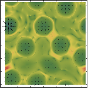



1. Introduction
1.1. Instabilities of Rayleigh–Taylor condensing layers
When a pure liquid layer of condensable species is hanging on a cooled horizontal substrate and in contact with its own vapour below, condensation can occur under the difference in vapour pressure (or chemical potential) between the gas side of the interface and its adjacent ambient if the substrate temperature remains below the saturation value. The pre-existing planar interface between the pendent liquid layer and the gas phase (with surface tension  $\sigma _0$ and density
 $\rho >\rho ^{(g)}$) is inherently unstable to infinitesimal deformations with gravity
 ${\boldsymbol {g}}$ directing to the lighter fluid (Fermigier et al. Reference Fermigier, Limat, Wesfreid, Boudinet and Quilliet1992; Oron & Rosenau Reference Oron and Rosenau1992; Burgess et al. Reference Burgess, Juel, McCormick, Swift and Swinney2001), known as the Rayleigh–Taylor instability (RTI) (Chandrasekhar Reference Chandrasekhar1981, Chapter X). The situation with a heavier, semi-infinite fluid on top of an immiscible, viscous film (Yiantsios & Higgins Reference Yiantsios and Higgins1989) is a counterpart. Independent of the initial thickness of the liquid layer and flow regime, the critical (shortest) wavelength of the RTI of a finite-thickness viscous layer is
 $\tilde {\lambda }_{{RT},c}=2 {\rm \pi}l_{c}$ with the capillary length
 $l_{c}=\sqrt {\sigma _0/[(\rho -\rho ^{(g)})\lvert g\rvert ]}$, below which the interface is stable according to the linear stability analysis. In the presence of phase change, the unstable film condensation of fundamental interest (Gerstmann & Griffith Reference Gerstmann and Griffith1967; Bestehorn & Merkt Reference Bestehorn and Merkt2006; Som et al. Reference Som, Kimball, Hermanson and Allen2007) is also one of the most important factors in heat exchangers of nuclear power plant and that of electric devices with high power density. For instance, in the gravity-assisted heat pipe studied by Yanadori et al. (Reference Yanadori, Hijikata, Mori and Uchida1985), the condensate falls as drops from a ceiling to complete a cooling cycle.
Contrarily, there are several different ways to inhibit the RTI. The purely dissipative RTI could be inhibited dynamically with an imposed harmonic oscillation upon the liquid, perpendicularly to the horizontal equilibrium state of the gas–liquid interface, as demonstrated experimentally by Wolf (Reference Wolf1970). It could also be suppressed thermally with a sufficient cooling by the bounding substrate because the Marangoni effect can act as a stabilization of the gas–liquid interface provided its surface tension increases as the temperature decreases, as predicted numerically (Deissler & Oron Reference Deissler and Oron1992; Oron & Rosenau Reference Oron and Rosenau1992; Alexeev & Oron Reference Alexeev and Oron2007) and verified experimentally by applying a vertical temperature gradient to a gas–liquid system (Burgess et al. Reference Burgess, Juel, McCormick, Swift and Swinney2001). However, the effect of thermocapillary flow is generally negligible for an evaporating or condensing layer in contact with its pure vapour (Guo & Narayanan Reference Guo and Narayanan2010; Kimball, Hermanson & Allen Reference Kimball, Hermanson and Allen2012) since phase change tends to drive the interfacial temperature towards an equilibrium value under the large enthalpy difference between the two phases (Kanatani Reference Kanatani2010), see also Chauvet, Dehaeck & Colinet (Reference Chauvet, Dehaeck and Colinet2012) for a concise theoretical explanation on phase-change-induced thermal spreading mechanism on an interface. Therefore, neglecting the Marangoni effects for a thermodynamic (quasi-)equilibrium interface is a reasonable simplification in pure-component systems (Haut & Colinet Reference Haut and Colinet2005; Kanatani Reference Kanatani2010; Wei & Duan Reference Wei and Duan2016). Moreover, Hsieh (Reference Hsieh1972) earlier proposed that RTI can be stabilized by the effects of heat and mass transfer associated with evaporation using linear stability analysis (LSA). Bestehorn & Merkt (Reference Bestehorn and Merkt2006) theoretically showed that a Rayleigh–Taylor unstable liquid layer could also be stabilized by localized evaporation and condensation with large enough mass fluxes and that the Rayleigh–Taylor-driven rupture could be avoided even without the stabilizing Marangoni effect provided the initial interface is in equilibrium with the vapour below.
Film condensation creates different temperature gradients at the gas and liquid sides of an interface as a consequence of the combined effects of the deposited latent heat at the interface, the convective/conductive heat fluxes in a vapour boundary layer and the heat conduction through the condensate layer (Fujii Reference Fujii1991). The temperature gradients are sustained by continuous removal of the heat via the cooled substrate. A mechanical perturbation on the interface will be weakened: as the liquid-side temperature gradient at a trough (closer to the cold substrate) becomes stronger while the gas-side temperature gradient gets weaker, the local condensation flux will increase since it is proportional to the difference in the interfacial heat fluxes. The opposite situation appears in a crest (more evaporative). This physical argument for the stabilizing effect of phase change applies to both positive and negative gravity cases regardless of surface-tension gradients. Accordingly, a significant temperature difference can be established across the liquid, especially in the relatively thicker region of a Rayleigh–Taylor unstable layer or in a hanging droplet (Savino, Paterna & Favaloro Reference Savino, Paterna and Favaloro2002), which could be sufficient for buoyancy effect in the liquid to destabilize the conductive motionless state besides the Marangoni effect. The resulting convection, in turn, can affect the evaporation/condensation rate. As concluded by Savino et al. (Reference Savino, Paterna and Favaloro2002), the numerical solutions for evaporation rates of both a pendent water and octane drop compared most favourably with experimental results when the buoyancy effect was included in simulations. In addition, it has also been shown that under positive gravity the thermal buoyancy can play a significant role in the evaporative convection of liquid layers with not-very-thin thicknesses, e.g.  $h\le 1$ mm trichlorotrifluoroethane (R-113) (Zhang Reference Zhang and Savino2006) and 2 mm water (Guo & Narayanan Reference Guo and Narayanan2010).
The striking phenomena of evaporative convection in pure liquid layers were observed by Berg, Boudart & Acrivos (Reference Berg, Boudart and Acrivos1966) who exploratively explained the patterns with simultaneous effects of thermocapillarity and buoyancy. In this study, we show the influence of buoyancy on the convection in pendent drops of a Rayleigh–Taylor unstable condensing layer. On the other hand, according to the interface mass balance, a rapidly approaching vapour ‘particle’ impinging on the interface must decelerate substantially as it becomes liquefied, which can produce a vapour recoil. The interfacial convection and heat-transfer characteristics associated with the vapour recoil instability have been studied experimentally by Hickman (Reference Hickman1952) and Palmer & Maheshri (Reference Palmer and Maheshri1981). With pseudo-steady LSA, Palmer (Reference Palmer1976) showed that the vapour recoil stemming from interfacial mass transfer acted as an important destabilizing effect of evaporation that caused interfacial convection at low ambient pressure. Further, Kliakhandler, Davis & Bankoff (Reference Kliakhandler, Davis and Bankoff2002) showed that the vapour recoil played a crucial stabilizing role in a falling film as it increased the critical Reynolds number from zero in isothermal cases to a positive value in condensing cases. Accordingly, we also account for the mechanisms of gravity combined with buoyancy in the liquid, vapour recoil on the interface and heat flux via the vapour in a general framework (in order to unify various cases in a consistent way, see Wei & Duan (Reference Wei and Duan2018)), the major concern of this work shall be the nonlinear effects of the interfacial convection and diffusion of vapour on pattern formation.
1.2. Nonlinear stability analysis: one-, two- and  $1.5$-sided models

The first comprehensive nonlinear analysis on evaporating and condensing liquid layers was performed by Burelbach, Bankoff & Davis (Reference Burelbach, Bankoff and Davis1988), who developed a long-wave (LW) evolution equation describing the dynamics of the gas–liquid interface of an ultra-thin film subject to the effects of thermodynamic non-equilibrium, disjoining pressure, mass loss/gain, vapour recoil, capillarity and thermocapillarity. By numerically integrating the evolution equation, they investigated the influences of these effects on rupture instability in  $(1+1)$-dimension (
 $(1+1)$-D). Here and in the following
 $(1+1)$ and
 $(2+1)$ denote the numbers of independent spatial plus temporal variables in evolution equation(s). Particularly, it was shown that an interfacial perturbation could enhance the condensation flux at a thinner region (as just mentioned) and thus locally normal stresses associated with vapour thrust (Burelbach et al. Reference Burelbach, Bankoff and Davis1988). Adopting a special potential for the intermolecular forces between an ultra-thin film and a coated substrate, Oron (Reference Oron2000b) numerically studied the
 $(2+1)$-D pattern formation in a horizontal evaporating film. Later, with the same potential function, Oron & Bankoff (Reference Oron and Bankoff2001) examined the interfacial and heat-flux evolution of a
 $(1+1)$-D condensing film on a horizontal or slightly inclined surface in different condensation paradigms. The last two works incorporate attractive–repulsive molecular forces, surface tension and mass loss/gain without hydrostatic effect owing to its vanishing influence in horizontal cases within the thickness range of interest, but including a gravity-driven effect in inclined cases in the latter. In these studies, the film dynamics is described by a nonlinear LW equation in the framework of a one-sided model, in which the dynamics of the vapour are decoupled from that of the liquid.
Some researchers used a two-sided model (e.g. Guo & Narayanan Reference Guo and Narayanan2010; Kanatani & Oron Reference Kanatani and Oron2011; Pillai & Narayanan Reference Pillai and Narayanan2018) to account for the mass, heat and/or viscous coupling between the two phases, which are numerically demanding for fully nonlinear  $(2+1)$-D cases. Recent work by Pillai & Narayanan (Reference Pillai and Narayanan2018) considered a binary volatile-liquid mixture lying above its vapour, confined between two plates and subjected to RTI and solutal Marangoni instability. Under thermodynamic equilibrium and LW approximation, the
 $(1+1)$-D dynamics was studied using the weighted-residual integral boundary layer method, which yielded a set of coupled nonlinear equations for the interface position and the flow rates of both phases. The simulation suggested that the stabilizing effect of mass transfer by phase change could overcome the destabilizing concentration gradients and RTI. Specifically, the solutal Marangoni effect was insufficient to result in a touching down of the interface on the hot vapour-side wall, because a reversed liquid flow along the interface could be driven by vapour convection associated with increasingly intense phase change in the stability competition. We neglect this effect to simplify the problem. A posteriori justification is supported by the results shown in figures 9(d), 11(d) and 12(d) (just not close to the final time in the last one), where the spatial variations of interfacial concentration are not too large, typically within
 ${O}(0.01)$.
Our model does not take into account the full dynamics in the gas phase but it does take into account convection and diffusion of vapour as well as heat transfer in the vicinity of the interface, and is thus referred to as a  $1.5$-sided model. It can also be reduced to a conventional one-sided model (Burelbach et al. Reference Burelbach, Bankoff and Davis1988) if the vapour transport on the interface owing to concentration variations can be disregarded (see § 2.3.3). Our research aims to employ the
 $1.5$-sided model to understand the dynamics of the Rayleigh–Taylor unstable condensing layers, by characterizing in detail the pattern formation and comparing to the relevant results of the one-sided model. This is also the novelty of the work. As can be seen later, the one-sided simulations for the condensing layer reveal that the interface can evolve into local rupture, while the
 $1.5$-sided model shows that the mechanisms of convection and diffusion of vapour play a significantly stabilizing role in suppressing the potential rupture.
1.3. Motivations
Most of the previous theoretical studies on interfacial instability and evaporative convection considered that a volatile liquid layer was in contact only with its own vapour (Palmer Reference Palmer1976; Burelbach et al. Reference Burelbach, Bankoff and Davis1988; Kliakhandler et al. Reference Kliakhandler, Davis and Bankoff2002; Guo & Narayanan Reference Guo and Narayanan2010; Kanatani Reference Kanatani2010; Kanatani & Oron Reference Kanatani and Oron2011) and that the atmosphere has a constant vapour pressure (Bestehorn & Merkt Reference Bestehorn and Merkt2006). Later, some numerical investigations have considered ambient gas as a mixture of the vapour and an inert (non-condensable) gas in the presence of vapour diffusion by linear or weakly nonlinear analysis (Haut & Colinet Reference Haut and Colinet2005; Margerit, Dondlinger & Dauby Reference Margerit, Dondlinger and Dauby2005; Sultan, Boudaoud & Amar Reference Sultan, Boudaoud and Amar2005). However, vapour convection has usually been either neglected or ignored, except for the LSA by Kanatani (Reference Kanatani2010, Reference Kanatani2013), the simulations by Kanatani & Oron (Reference Kanatani and Oron2011) and Pillai & Narayanan (Reference Pillai and Narayanan2018) and the experimental and numerical studies in Savino et al. (Reference Savino, Paterna and Favaloro2002) and Dehaeck, Rednikov & Colinet (Reference Dehaeck, Rednikov and Colinet2014). As suggested by Kanatani (Reference Kanatani2013) and Pillai & Narayanan (Reference Pillai and Narayanan2018), to predict what actual patterns emerge from an evaporating film or whether instabilities lead to its rupture, a nonlinear computation is required, because of the time and thickness dependence of the maximum growth mode in the LSA. To our knowledge, there are relatively few works (Kanatani & Oron Reference Kanatani and Oron2011; Pillai & Narayanan Reference Pillai and Narayanan2018) focusing on the nonlinear effects of vapour transport on the interface stability of a liquid layer with phase change, among which Kanatani & Oron (Reference Kanatani and Oron2011) investigated a  $(1+1)$-D liquid–vapour system but neglected net mass flux and vapour recoil based on a model derived earlier (Kanatani Reference Kanatani2010).
Although the amount of research in this field is growing recently, the majority of the theoretical works on evaporating/condensing layers is based on the  $(1+1)$-D computation of a one-sided model, which could provide a qualitative prediction of the interfacial dynamics (Oron Reference Oron2000b) under proper conditions. Moreover, there are few investigations of the nonlinear evolution of liquid layers with phase change incorporating both the effects of convection and diffusion of vapour among others, as introduced above, since it is still difficult to develop and/or solve a fully nonlinear, unsteady two-sided model, especially for
 $(2+1)$-D cases. Therefore, an appropriately reduced model awaits its realization.
The nonlinear dynamics and stabilities of the gas–liquid interface of a liquid layer with phase change are by no means fully understood because of, for instance, the complexity in the thermodynamic condition and the frequent coexistence of diffusion and convection of vapour near the interface. The essential factors that influence the vapour convection along the interface can be (i) phase-change-induced gas bulk flow within an open or confined geometry (Kanatani Reference Kanatani2013; Pillai & Narayanan Reference Pillai and Narayanan2018); (ii) phase-change-induced lateral variations of vapour pressure near the interface (Kanatani & Oron Reference Kanatani and Oron2011); (iii) interfacial thermal Marangoni flow in the liquid (Savino et al. Reference Savino, Paterna and Favaloro2002; Dehaeck et al. Reference Dehaeck, Rednikov and Colinet2014); and (iv) thermal and/or solutal buoyancy effects in the gas phase (Savino et al. Reference Savino, Paterna and Favaloro2002; Som et al. Reference Som, Kimball, Hermanson and Allen2007; Guo & Narayanan Reference Guo and Narayanan2010; Dehaeck et al. Reference Dehaeck, Rednikov and Colinet2014). In the condensing case, a concentration boundary layer can be built up with a minimum (maximum) concentration for condensable (non-condensable) species at the interface because of the bulk condensing flow of ambient towards the interface (see figure 1). Also, the increases in mean (due to mass gain) and local (due to instabilities) thicknesses make non-trivial effects of heat transfer in the gas phase possible if the latent heat  $(\tilde{L})$ of a liquid is not too large, e.g.
 $\tilde {L}_{\textrm {R}\text {-}113}\approx 150\ \textrm {kJ}\,\textrm {kg}^{-1}$ and
 $\tilde {L}_{ethanol}=878\ \textrm {kJ}\,\textrm {kg}^{-1}$ at
 $300$ K. For film condensation on the underside of a horizontal surface, these considerations motivate us to introduce a concentration–thermal vapour boundary layer (VBL) to model the convection and diffusion of vapour as well as heat transfer near the interface. This is similar to that proposed by Haut & Colinet (Reference Haut and Colinet2005) (they incorporated also a viscous boundary layer) and that applied by Kanatani (Reference Kanatani2013) and Dehaeck et al. (Reference Dehaeck, Rednikov and Colinet2014) (the latter considered a concentration–viscous boundary layer). With pseudo-steady LSA, Haut & Colinet (Reference Haut and Colinet2005) studied the influence of an inert gas on evaporation-induced Bénard–Marangoni convection; Kanatani (Reference Kanatani2013) considered a concentration boundary layer without heat flux in the gas and focused on the linear stability of an evaporating interface. Particularly, the latter predicted that the stabilizing effect of the rate of change of the interfacial vapour concentration could be significant for rapidly growing perturbations and thicker regions in a film. This motivates a full nonlinear simulation in the context of a Rayleigh–Taylor unstable condensing layer.
Schematic of film condensation on the underside of a cooled horizontal substrate ( $\theta _{w}<\theta _\infty$) in the presence of a vapour boundary layer of thickness
 $\delta$. The molar fractions of the vapour and the non-condensable gas are denoted as
 $\tilde {x}_{A}$ and
 $\tilde {x}_{B}$. The wavelength of a typical interfacial disturbance
 $\tilde {\lambda }$ is the horizontal characteristic length, much larger than the average liquid thickness
 $h_{av}$. A smaller dot in the bulge of the liquid layer represents a lighter fluid particle (not in scale), allowing for the buoyancy effect.

Extensive experimental and theoretical studies have been conducted on condensation heat transfer in vertical falling and horizontal hanging condensate films of pure or multi-component vapour in the presence or absence of an inert gas (Kroger & Rohsenow Reference Kroger and Rohsenow1968; Yanadori et al. Reference Yanadori, Hijikata, Mori and Uchida1985; Fujii Reference Fujii1991; Kliakhandler et al. Reference Kliakhandler, Davis and Bankoff2002; Som et al. Reference Som, Kimball, Hermanson and Allen2007). The earliest attempts at predicting the interfacial characteristic dimensions and heat-transfer rates of a film condensation of pure vapour on the underside of horizontal and inclined plates were made by Gerstmann & Griffith (Reference Gerstmann and Griffith1967, referred to herein as GG). They assumed the flow to be steady and periodic (in the longitudinal direction of the slope). The calculated average Nusselt number agreed well with their experiments of horizontal and slightly inclined cases. However, their assumptions caused an approximately  $25$ % underestimation on the wavelength of the instabilities. Later, Yanadori et al. (Reference Yanadori, Hijikata, Mori and Uchida1985) considered a similar problem using much smaller circular surfaces to correlate the optimum heat-transfer performance with RTI wavelength, and explained the results with a ratio of the thin-film area to the total condensing area. By varying vapour pressure and wall temperature, Som et al. (Reference Som, Kimball, Hermanson and Allen2007) made an experimental study on the stability and heat flux of a cyclically condensing–evaporating layer of
 $n$-pentane on the underside of a horizontal wall. The common feature of these investigations is that the heat-transfer characteristics are altered greatly by RTI. Nevertheless, theoretical studies addressing the problem of interfacial stability in Rayleigh–Taylor unstable evaporating/condensing layers, especially the
 $(2+1)$-D dynamics in the presence of non-condensable species, are still limited in the literature. Thus a fundamental research is crucial to understand how the complicated interfacial phenomena are affected by the relevant mechanisms involved in the heat and mass transfer processes. The overall objective of the current research is to examine the dynamics in such a case, especially under the influences of convection and diffusion of the vapour.
We will improve the model of an evaporating layer in the same spirit as the heuristic works (Haut & Colinet Reference Haut and Colinet2005; Kanatani Reference Kanatani2013), where LSA were carried out to investigate the short-wave convective instability with an undeformable flat surface (Haut & Colinet Reference Haut and Colinet2005) and the LW interfacial instability with an deformable surface (Kanatani Reference Kanatani2013). In this study, we shall concentrate on the pattern formation and interfacial stability of a Rayleigh–Taylor unstable filmwise condensation, where the stabilizations of liquid viscosity, surface tension and the Marangoni effect compete with the destabilizing mechanisms of vapour recoil and gravity combined with buoyancy. We consider that the ambient consists of the vapour of a volatile liquid and an inert gas, because not only can the presence of an inert component strongly stimulate the thermal Marangoni effect but also it is the general case in experiments. Under this circumstance, the fluctuation of vapour pressure can give rise to temperature variations along the gas–liquid interface, even though it is in local equilibrium with adjacent ambient, see Haut & Colinet (Reference Haut and Colinet2005) for example. In addition, the effects of vapour convection near the interface allow higher mass fluxes (Savino et al. Reference Savino, Paterna and Favaloro2002; Kanatani Reference Kanatani2013; Dehaeck et al. Reference Dehaeck, Rednikov and Colinet2014) as compared to that of pure diffusion-limited cases, e.g. in Haut & Colinet (Reference Haut and Colinet2005) and Sultan et al. (Reference Sultan, Boudaoud and Amar2005), since a lower limitation of mass flux can be set by the pure diffusion of vapour through an inert gas. This also provides a justification for retaining the effect of vapour recoil in the present study.
The organization of this paper is as follows. In § 2, we derive the  $1.5$-sided model along with the reduced one-sided model. In § 3, we formulate an extended basic state, which is studied with pseudo-steady approximation. In § 4, we investigate the linear stability of the basic state with frozen-time approach and explain the relevant stabilizing mechanisms with a simplified case. In § 5, we summarize the models to be solved and outline the numerical methods. In § 6, the numerical results of both models in representative cases are presented, which are compared with each other and with experiments from the literature. The effects of VBL thickness and initial interface concentration are also briefly discussed with a time-dependent basic state. In § 7, we examine the competition between the stabilizing effect of thermocapillarity and the destabilizing effect of gravity. This section ends with the discussion of a disturbance thermal energy equation. Finally, concluding remarks are summarized in § 8.
2. Mathematical formulation
2.1. Physical description and governing equations
We consider a laterally unbounded condensing layer of species A on the underside of a horizontal, uniformly cooled solid substrate at a constant temperature,  $\theta _{w}$. As depicted in figure 1, the liquid layer, subject to RTI in a gravitational field, is bounded from below by a binary mixture of its vapour A and a non-condensable inert gas of species B. It is assumed that the system is completely wetting and the inert gas B is not absorbed into the condensate A. The gas is considered to be ideal and incompressible. The liquid is colder than its semi-infinite surrounding that condensation occurs on the gas–liquid interface. The Marangoni stresses due to interfacial temperature gradients (through fluctuations of local liquid thickness and vapour concentration) and the buoyancy forces due to adverse density gradients (energized by vertical temperature differences) could simultaneously affect the convection of the liquid. However, the effects of buoyancy are negligible in the nearby gas with small density variations, provided the concentration and temperature differences are not too large and the molar masses of vapour and inert species are of the same order, as in the studied system.
In a typical binary gas–liquid system, the Lewis number,  $Le^{(g)}=\alpha ^{(g)}/D_{AB}={O}(1)$, with
 $\alpha ^{(g)}$ and
 $D_{AB}$ being the thermal and binary diffusivities of the gas mixture. This permits an asymptotic characterization of interfacial heat and mass transfer by introducing a concentration–thermal vapour boundary layer of a thickness
 $\delta$ between the pure liquid layer and the perfectly mixed bulk gas, as mentioned in § 1.3. That is, on the outer boundary of the VBL the temperature, pressure and vapour concentration are taken to be the uniform bulk values,
 $\theta _\infty (>\theta _{w})$,
 $p_0$ and
 $\tilde {x}_{{A}\infty }$ with
 $\tilde {x}_i$ denoting the molar fraction of species
 $i=\{{A}, {B}\}$ and subscript ‘
 $\infty$’ for the bulk quantities. For simplicity we adopt Cartesian coordinates
 $(x,z)$ to formulate the liquid–VBL bilayer system without loss of generality, provided forces and perturbations are isotropic in the horizontal directions,
 $\boldsymbol {x}=(x,y)$ (the
 $y$-coordinate lying in the substrate and normal to
 $x$). The gas–liquid interface is located at
 $z=h(x,t)$, which evolves in time
 $t$ from an initially average thickness,
 $h_0\equiv h_{av}(t=0)$. The unit vector normal to the interface and directed towards the gas phase is given by
 $\boldsymbol {n}=(-\partial _x h,1)[1+(\partial _x h)^2]^{-1/2}$, and
 $\boldsymbol {t}=(1,\partial _x h)[1+(\partial _x h)^2]^{-1/2}$ is the unit tangent vector to the interface.
As shown in figure 1, the total gas pressure  $p_0$ is supposed to be constant (Haut & Colinet Reference Haut and Colinet2005), and
 $p_{A}$ is the local value of partial pressure of vapour which reaches a uniform value,
 $p_{{A}\infty }=p_0\tilde {x}_{{A}\infty }$, at the outer boundary of VBL. Let
 $\theta _{{A},s}(p)$ be the saturation temperature, at which the liquid and its vapour coexist when both are at a common pressure
 $p$. The coexistence pressure
 $p_{s}(\theta )$ is defined as the partial pressure of the vapour required for the liquid to coexist with its vapour at the temperature
 $\theta$. Precisely,
 $\theta _{{A},s}$ and
 $p_{s}$ are linked by the Clausius–Clapeyron law,
 \begin{equation} p_{s}(\theta)= p_0\exp [\bar{L}R^{-1} (\theta_{{A},s}^{-1}(p_0)-\theta^{-1})]. \end{equation}
Here,  $\bar {L}=M_{A}\tilde {L}$, in which
 $\tilde {L}$ and
 $\bar {L}$ are the specific and molar latent heats of species A with
 $M_{A}$ being its molar mass; the universal gas constant
 $R=8.3145 \ \textrm {J}\,\textrm {mol}^{-1}\,\textrm {K}^{-1}$;
 $p_0$ is chosen as the reference pressure of a thermodynamic equilibrium. If the interface is in equilibrium, the actual partial pressure at the interface is equal to the saturation pressure at the interfacial temperature; that is,
 $p_{A,I}=p_{s}(\theta _{I})$, with the subscript ‘I’ denoting quantities evaluated on the interface. The saturated molar fraction at the interface is given by
 $\tilde {x}_{A,I,eq}=p_{s}(\theta _{I})/p_0$, with the subscript ‘eq’ denoting the local equilibrium value.
The bulk properties of the ambient are calculated with the ideal gas model (appendix A). Considering  $\delta \gg h$, we can assume that
 $\delta$ does not change appreciably with the evolution of
 $h$ over the length and time scales in the LW limit. Moreover, a reference body force
 $\boldsymbol {F}_{rb}=-\boldsymbol {\nabla } \phi$, with a gravitational potential
 $\phi =\rho g z$, is defined to incorporate the buoyancy effect in the condensate layer, where
 $\boldsymbol {\nabla }= (\partial _x,\partial _z)$,
 $\rho$ is the liquid density at the reference temperature
 $\theta _{w}$ and
 $g$ is the negative gravitational acceleration.
The liquid layer consists of a pure Newtonian fluid of constant physical properties except for the temperature dependence of the saturation conditions (as mentioned earlier), surface tension and density. The gas–liquid interfacial tension is represented as  $\sigma =\sigma _0-\gamma (\theta -\theta _{w})$ with the reference value
 $\sigma _0$ at
 $\theta _{w}$ and
 $\gamma =-(\text {d}\sigma /\text {d}\theta )_{\theta _{w}}>0$. With the Boussinesq approximation and the other non-Boussinesq effects neglected (Velarde, Nepomnyashchy & Hennenberg Reference Velarde, Nepomnyashchy and Hennenberg2001), the continuity, momentum and energy equations for the liquid layer read
 \begin{gather} \boldsymbol{\nabla}\boldsymbol{\cdot}\boldsymbol{v} = 0, \end{gather}
 \begin{gather}\rho(\partial_t\boldsymbol{v}+\boldsymbol{v}\boldsymbol{\cdot}\boldsymbol{\nabla}\boldsymbol{v}) = -\boldsymbol{\nabla} p+\mu\nabla^{2}\boldsymbol{v}-\rho[1-\beta(\theta-\theta_{w})]g\boldsymbol{e}_z, \end{gather}
 \begin{gather}\rho c_p(\partial_t\theta+\boldsymbol{v}\boldsymbol{\cdot} {\boldsymbol{\nabla}} \theta) = k^{(l)}\nabla^2\theta, \end{gather}
where  $\nabla ^2=\boldsymbol {\nabla }\boldsymbol {\cdot }\boldsymbol {\nabla }$ is the Laplacian;
 $\boldsymbol {v}=(u, w)$,
 $p$ and
 $\theta$ are the velocity, pressure and temperature of the liquid, and
 $\boldsymbol {e}_z$ is the unit vector in the
 $z$-direction. The physical properties of the liquid,
 $\mu$,
 $\beta$,
 $c_p$ and
 $k^{(l)}$, are, respectively, dynamic viscosity, thermal expansion coefficient (assuming
 $\beta >0$), specific heat capacity and thermal conductivity, taken at
 $\theta _{w}$. The last term on the right-hand side of (2.3) incorporates the variation in density with temperature, responsible for buoyancy-driven convection in the non-isothermal liquid layer. The mass conservation for the incompressible gas mixture and species conservation of the volatile component in the VBL can be written as
 \begin{gather} {\boldsymbol{\nabla}}\boldsymbol{\cdot}\boldsymbol{v}^{(g)} = 0, \end{gather}
 \begin{gather}\partial_t\tilde{x}_{A}+\boldsymbol{v}^{(g)}\boldsymbol{\cdot}{\boldsymbol{\nabla}} \tilde{x}_{A} = D_{{AB}}\nabla^{2}\tilde{x}_{A}. \end{gather}
Here,  $\boldsymbol {v}^{(g)}=(u^{({g})}, w^{({g})})$ is the mass-average velocity of the gas mixture and the species flux due to thermal diffusion has been neglected in (2.6). We do not need momentum equations for the gas phase since a viscous boundary layer is not our concern. The molar fraction,
 $\tilde {x}_i$, is related to the total and partial molar concentrations of the gas mixture,
 $C$ and
 $C_i^{({g})}$, by
 $\tilde {x}_i=C_i^{({g})}/C=C_i^{({g})}/\sum _{i}C_i^{({g})}$. In addition, the simple form of (2.5) and (2.6) implies that the total mass and molar concentrations,
 $\rho ^{(g)}$ and
 $C$, of the gas mixture are assumed to be constant, consistent with the neglect of buoyancy convection in the VBL (appendix E). Thereafter, superscripts ‘l’ and ‘g’ are used to distinguish the liquid and gas quantities if necessary. We have expressed the gas concentration in molar units (e.g. mol m
 $^{-3}$) and employed the molar fraction in (2.6) instead of the mass fraction, because problems involving a mixture of chemical species are handled more easily with molar quantities (see e.g. Dehaeck et al. Reference Dehaeck, Rednikov and Colinet2014). For instance, it is more convenient to calculate the partial pressure with the molar fraction. The properties of a typical ethanol–nitrogen system are listed in table 1 and assumed to be constant. This is reasonable for an isobaric ambient with
 $M_{A}/M_{B}={O}(1)$ and small-to-moderate variations in concentration and temperature.
Physical properties for the ethanol–nitrogen system at  $\theta _{w}=300$ K or
 $\theta _\infty =330$ K and
 $p_0=101$ kPa. All unannotated data are adopted from Haut & Colinet (Reference Haut and Colinet2005).

 $^{a}$Dittmar et al. (Reference Dittmar, Fredenhagen, Oei and Eggers2003).
 $^{b}$Estimated using (A 2) and (A 3) with
 $\tilde {x}_{{A}\infty }=0.2$.
 $p_{{A}\infty }=\tilde {x}_{{A}\infty }p_0=20.2$ kPa and the relative humidity of ambient,
 $\varphi _\infty =p_{{A}\infty }/p_{s}(\theta _\infty )=0.494$. This is an unsaturated gas, whose saturated molar fraction,
 $\tilde {x}_{{A}\infty ,{eq}}=0.409$, can be calculated by (2.1).
 $^c$NIST Standard Database 23, Version 8.0.
 $^d$Equilibrium value obtained with (2.1) at
 $\theta _{w}$.
 $^e$Estimated with the Dalton's law of partial pressure for ideal gas,
 $p_{s}(\theta _{w})=p_0\tilde {x}_{A,w}$.
At the liquid–solid interface,  $z=0$, we apply the no-slip, no-penetration and constant temperature conditions:
 $u = w = 0$ and
 $\theta =\theta _{w}$. The balance of mass and molar fluxes of the volatile component at the interface,
 $z=h(x,t)$, read
 \begin{gather} j(x,t) = \rho(\boldsymbol{v}_{I}-\boldsymbol{v})\boldsymbol{\cdot}\boldsymbol{n} = \rho^{({g})}(\boldsymbol{v}_{I}-\boldsymbol{v}^{(g)})\boldsymbol{\cdot} \boldsymbol{n}, \end{gather}
 \begin{gather}N_{{An}}^{({g})}(h,t)=\boldsymbol{J}_{{A,I}}^{{(M)}}\boldsymbol{\cdot}\boldsymbol{n}+ C_{{A}}^{({g})}\boldsymbol{v}^{({g},{M})}\boldsymbol{\cdot}\boldsymbol{n} =-CD_{AB}\boldsymbol{\nabla}\tilde{x}_{A,I}\boldsymbol{\cdot}\boldsymbol{n}+ \tilde{x}_{A,I} N_{{An}}^{({g})}(h,t), \end{gather}
where  $j$ is the local mass flux normal to the interface (
 $j>0$ for condensation);
 $\boldsymbol {v}_{I}$ is the interface velocity; as
 $\boldsymbol {N}_i$ represents the molar flux of species
 $i$,
 $N_{{An}}^{(g)}$ is its normal component of species A in gas phase;
 $\boldsymbol {J}_i^{{(M)}}$ is the molar diffusional flux relative to the molar-average velocity
 $\boldsymbol {v}^{({g},{M})}=\sum _{i}\tilde {x}_i\boldsymbol {v}_i^{({g})}$, where
 $\boldsymbol {v}_i^{({g})}=\boldsymbol {N}_i^{({g})}/C_i^{({g})}$ is the velocity of species
 $i$ relative to a fixed origin. The one-component conservation law (2.8) has been expressed in molar units with the diffusional reference frame
 $\boldsymbol {v}^{({g},{M})}$, which follows the preferred form of Fick's law since for a gas mixture at uniform pressure, it is more usual to have a constant
 $C$ rather than
 $\rho ^{({g})}$, especially when the difference between the molar mass of A and B is large (see e.g. the supporting information of Dehaeck et al. Reference Dehaeck, Rednikov and Colinet2014). Equation (2.8) thus is a more accurate counterpart to the flux balance in mass units (see (2.13) in Kanatani Reference Kanatani2013). Here, the flux of species
 $B$ is negligible and
 $N_{{An}}^{({g})}<0$ for condensation, which will be clarified in § 3.1. Accordingly, the mass and molar fluxes are related through
 $j=-M_{A}N_{{An}}^{({g})}$. It should be mentioned that the two terms on the right-hand side of (2.8) account for the diffusion and convection of the condensable species normal to the interface, respectively. The latter, induced by the condensing bulk flow, has been neglected in most studies, which is similar to but different from that used by Kanatani (Reference Kanatani2013), because exactly how much of the flux is attributed to convection and to diffusion depends upon the choice of the reference velocity. Henceforth, the subscript ‘n’ refers to quantities projected in the normal direction of the interface. Furthermore, in the presence of mass transfer the interface satisfies the kinematic condition,
 \begin{equation} j=\rho[1+(\partial_x h)^2]^{-1/2}(\partial_th+u\partial_x h-w). \end{equation}
The interfacial balance relations for energy and stresses and the continuity of tangential velocities read,
 \begin{gather} j\tilde{L}+h_{{th}}(\theta_\infty-\theta) = k^{({l})}\boldsymbol{\nabla} \theta \boldsymbol{\cdot} \boldsymbol{n}, \end{gather}
 \begin{gather}j(\boldsymbol{v}^{({g})}-\boldsymbol{v})+(p-p_0)\boldsymbol{n}-2\mu\boldsymbol{\varGamma}\boldsymbol{\cdot} \boldsymbol{n} +2\kappa\sigma\boldsymbol{n}+\boldsymbol{\nabla}_{\!s}\sigma = 0 , \end{gather}
 \begin{gather}(\boldsymbol{v}^{({g})}-\boldsymbol{v})\boldsymbol{\cdot}\boldsymbol{t}=0, \end{gather}
where  $\boldsymbol {\varGamma }={\textstyle \frac {1}{2}}[\boldsymbol {\nabla }\boldsymbol {v}+(\boldsymbol {\nabla }\boldsymbol {v})^{\textrm {T}}]$ represents the rate-of-strain tensor evaluated on liquid side of the interface and the mean curvature
 $\kappa$ of the interface is given by
 $2\kappa =-\boldsymbol {\nabla }_{s}\boldsymbol {\cdot } \boldsymbol {n}$ with the surface gradient operator
 $\boldsymbol {\nabla }_{s}$. Formally, we have taken the partial ‘one-sided’ limit (appendix A):
 $\rho ^{({g})}/\rho \rightarrow 0$ and
 $\mu ^{({g})}/\mu \rightarrow 0$, but never apply
 $k^{(g)}/k^{(l)}\rightarrow 0$, as considered by Kliakhandler et al. (Reference Kliakhandler, Davis and Bankoff2002), Haut & Colinet (Reference Haut and Colinet2005), Zhang (Reference Zhang and Savino2006) and Doumenc et al. (Reference Doumenc, Boeck, Guerrier and Rossi2010) in either condensation or evaporation cases. For a small (dimensionless) thickness (
 ${\varDelta }=\delta /h_0$) of a similar VBL (Haut & Colinet Reference Haut and Colinet2005), it has been shown that as the mean thickness of a liquid layer changes (e.g.
 $h_{av}$ thickens by condensation) the heat and mass transfer through the VBL can have a considerable impact on heat conduction in the liquid even when
 $D_{AB}={O}(10^{-5})\ \textrm {m}^{2}\,\textrm {s}^{-1}$ and
 $k^{(g)}/k^{(l)}={O}(0.1)$, provided
 $Le^{(g)}={O}(1)$. Specifically, in an evaporating ethanol–nitrogen system, Haut & Colinet (Reference Haut and Colinet2005) showed that with
 ${\varDelta }={O}(0.1)$ a decrease in
 ${\varDelta }$ (i.e. the resistance of VBL to heat and concentration diffusion,
 $R_{d}^{(g)}$) can diminish the resistance to heat conduction through the liquid,
 $R_{c}^{(l)}$. The kinetic energy of vapour particle and viscous dissipation have been neglected in (2.10). The viscous stress resulting from gas motion is negligible in (2.11). These effects were studied by Palmer (Reference Palmer1976) for a rapidly evaporating interface. As simplified by Doumenc et al. (Reference Doumenc, Boeck, Guerrier and Rossi2010) for an evaporating case, the second left-hand side term of (2.10) represents the conductive/convective heat fluxes through gas with a heat-transfer coefficient
 $h_{th}$ since our major concern is the interfacial dynamics instead of a detailed description of the heat transfer in the gas phase. The vapour-recoil effect is preserved in (2.11), proportional to the first left-hand side term. However, vapour recoil and heat flux in the gas were neglected in Kanatani (Reference Kanatani2013) under the assumption of slow evaporation without a thermal boundary layer. The normal and tangent components of (2.11) then become
 \begin{gather} -j^2/\rho^{({g})}+p-p_0-2\mu \boldsymbol{n} \boldsymbol{\cdot} \boldsymbol{\varGamma} \boldsymbol{\cdot} \boldsymbol{n}+2\kappa\sigma=0, \end{gather}
 \begin{gather}-2\mu \boldsymbol{n} \boldsymbol{\cdot} \boldsymbol{\varGamma} \boldsymbol{\cdot} \boldsymbol{t}+\boldsymbol{\nabla}_{\!s}\sigma\boldsymbol{\cdot}\boldsymbol{t}=0, \end{gather}
where  $\rho ^{({g})}/\rho \rightarrow 0$ and (2.12) have been substituted.
Finally, the Hertz–Knudsen–Schrage equation (Schrage Reference Schrage1953)
 \begin{equation} j=\hat{a}\sqrt{M_{A}/(2{\rm \pi} R \theta_{I})}[p_{A,I}-p_{s}(\theta_{I})], \end{equation}
is used as a constitutive relationship to close the system. Here,  $\hat {a}=2a/(2-a)$ with
 $a$ being the accommodation coefficient (
 $0<a\leq 1$). For
 $a\ll 1$, (2.14) reduces to the classical Hertz–Knudsen equation with
 $\hat {a}\approx a$, which is the physical situation of concern in this work. The standard constitutive equation is further linearized about
 $\theta _{w}$ and
 $\tilde {x}_{A,w}\equiv \tilde {x}_{A}(\theta _{w},p_0)$ of thermodynamic equilibrium (Kanatani Reference Kanatani2013). Again, we use molar units (cf. appendix B) and then substitute (B 1) and (B 2) into (2.14) to obtain
 \begin{equation} j=\hat{a}\left[p_0(\tilde{x}_{A,I}-\tilde{x}_{A,w})-\frac{p_{s}(\theta_{w})\bar{L}}{R\theta_{w}^2} (\theta_{I}-\theta_{w})\right] \sqrt{\frac{M_{A}}{2{\rm \pi} R \theta_{w}}}, \end{equation}
where the square-root term is evaluated at  $\theta _{w}$ as
 $\vert \theta _{I}-\theta _{w}\vert /\theta _{I}\ll 1$ in practice. The effect of deviation from local equilibrium at the gas–liquid interface is related to
 $\theta _{I}$ and
 $\tilde {x}_{A,I}$ through the local variations in
 $p_{s}$ and
 $p_{A}$, respectively, if the mass flux is modelled with this linearized expression (2.15). For weak or moderate mass flux (
 $0<E\ll 1$, see table 2) as consistent with the linearization, the possibility of temperature discontinuities across the interface is negligible (Ward & Stanga Reference Ward and Stanga2001). It is therefore reasonable to assume temperature continuity at the interface, i.e.
 $\theta ^{(l)}_{I}=\theta ^{({g})}_{I} (\equiv \theta _{I})$.
Relevant dimensionless groups evaluated using the properties in table 1 with  $h_0=0.5$ mm,
 $\tilde {x}_{{A}\infty }=0.2$ and
 $g=-9.8\ \textrm {m}\,\textrm {s}^{-2}$.

 $^{a}$Estimated by
 $Bi={k^{(g)} h^\star }/({k^{(l)} \delta })$ (see discussion following (3.18a,b)) with
 $\delta =5$ mm (see figure 3 in Dehaeck et al. Reference Dehaeck, Rednikov and Colinet2014),
 $h^\star$ being taken as the capillary length
 $l_{c}\approx 2$ mm, and
 $k^{(g)}=0.027\ \textrm {W}\,\textrm {m}^{-1}\,\textrm {K}^{-1}$ (appendix A). Alternatively,
 $Bi=0.011$ is applicable to the heat-transfer coefficient of
 $h_{th}=0.85\ \textrm {W}\,\textrm {m}^{-2}\,\textrm {K}^{-1}$ measured within a thin vapour layer of constant temperature gradient above a
 $1$ mm evaporating ethanol or R-113 (Zhang Reference Zhang and Savino2006).
 $^{b}$Estimated with
 $\hat {a}\approx a=0.01$ (Haut & Colinet Reference Haut and Colinet2005).
2.2. Model for vapour concentration at the interface
According to the mass and molar flux balances, (2.7) and (2.8), the condensation velocity of gas,  $v_{cond}$, and the normal component of
 $\boldsymbol {\nabla }\tilde {x}_{{A,I}}$ may be written as
 \begin{gather} v_{cond} \equiv j/\rho^{({g})}\approx-\boldsymbol{v}^{({g})}\boldsymbol{\cdot}\boldsymbol{n}, \end{gather}
 \begin{gather}\boldsymbol{\nabla}\tilde{x}_{A,I}\boldsymbol{\cdot}\boldsymbol{n} = -(1-\tilde{x}_{A,I})N_{An}^{(g)}/(CD_{AB}). \end{gather}
In (2.16) it has been assumed that  $|\boldsymbol {v}_{In}|\ll |\boldsymbol {v}_n^{(g)}|$ for estimation of vapour convection. This is also consistent with the consideration of vapour recoil. Assuming the variation of
 $\tilde {x}_{A}$ due to interfacial deformation is localized on the vapour side of the interface (Kanatani Reference Kanatani2013), we can take the limit
 $z\rightarrow h^+$ of (2.6), then substitute (2.12), (2.16) and (2.17) to obtain
 \begin{equation} \partial_t\tilde{x}_{A,I}+u_{I}\partial_x\tilde{x}_{A,I} -\frac{(1-\tilde{x}_{A,I})j^2}{\rho^{({g})}CD_{{AB}}M_{A}}= D_{{AB}}(\partial_x^2\tilde{x}_{A,I}+ \partial_z^2\tilde{x}_{A}\vert_{z=h^+} ), \end{equation}
in which the assumption of  $\lvert \partial _x h \rvert \ll 1$ has been used, which is valid in the long-wave regime (Oron, Davis & Bankoff Reference Oron, Davis and Bankoff1997), and the horizontal velocity on the liquid side of the interface,
 $u_{I}$, will be calculated later. Here, the vertical diffusion term on the vapour side of the interface can be approximated via a basic-state VBL concentration profile (using (3.14) and (3.16)),
 \begin{equation} \partial_z^2\bar{\tilde{x}}_{A}\vert_{z=\bar{h}} =-(1-\bar{\tilde{x}}_{A,I})CM_{A}/\rho^{({g})} (\delta^{-1}\ln\bar{\eta})^2, \end{equation}
where the overbar denotes basic-state variables (cf. § 3),  $\eta =(1-\tilde {x}_{{A}\infty })/(1-\tilde {x}_{A,I})$ and
 $\bar {\eta }$ is evaluated with
 $\bar {\tilde {x}}_{{A,I}}$. It is also valid for a deformed interface provided (i) the long-scale limit
 $\partial _x u^{(g)}\ll 1$ holds; and (ii) the ratio of characteristic velocity variations
 ${\rm \Delta} w^{(g)}/{\rm \Delta} u^{(g)}\ll 1$, a consequence of the geometric condition of
 $\delta /\tilde {\lambda }\ll 1$, as revealed by the continuity (2.5). Using (2.19) to model
 $\partial _z^2\tilde {x}_{A}\vert _{z=h^+}$, (2.18) becomes
 \begin{equation} \frac{\partial_t\tilde{x}_{A,I}+u_{I}\partial_x\tilde{x}_{A,I}}{D_{AB}} -\partial_x^2\tilde{x}_{A,I}= \frac{1-\tilde{x}_{A,I}}{\rho^{(g)}} \left[\frac{j^2}{CD_{AB}^2M_{A}} -CM_{A}\left(\frac{1}{\delta} \ln \eta \right)^2 \right]. \end{equation}
Equation (2.20) is the surface convection–diffusion equation for vapour concentration and is expected to hold for a deformed interface in the first approximation. The second and third left-hand side-terms are associated with the convective and diffusive transport in the  $x$-direction, while the two terms on the right-hand side represent those in the
 $z$-direction, respectively.
2.3. Non-dimensionalization and evolution equations
2.3.1. Dimensionless equations and parameters
We introduce the scalings for dimensionless variables,
 \begin{align} \left. \begin{array}{c} \displaystyle (X,Z,H,\varDelta)=h_0^{-1}(x,z,h,\delta), \quad T = \nu h_0^{-2} t,\quad (P,\varPhi)=h_0^2 \rho^{-1} \nu^{-2}(p-p_0,\phi),\\ \displaystyle \boldsymbol{V}=(U,W) = h_0 \nu^{-1}(u, w), \quad (J,\varTheta)=(\rho^{(g)}\sqrt{\hat{M}}D_{AB})^{-1} (h_0\,j, k^{(l)}(\theta-\theta_{w})\tilde{L}^{-1}), \end{array}\right\} \end{align}
where  $\alpha =k^{(l)}/(\rho c_p)$,
 $\nu =\mu /\rho$ and
 $Pr=\nu /\alpha$ are the thermal diffusivity, kinematic viscosity and Prandtl number of the liquid. The resulting non-dimensional groups and their values are listed in table 2. Substitution of the scalings into the governing system (2.2)–(2.4) of the liquid layer yields
 \begin{gather} \boldsymbol{\nabla}_{XZ}\boldsymbol{\cdot}\boldsymbol{V} = 0, \end{gather}
 \begin{gather}\partial_T U+ \boldsymbol{V}\boldsymbol{\cdot} \boldsymbol{\nabla}_{XZ}U = -\partial_X P + \nabla^2_{XZ}U, \end{gather}
 \begin{gather}\partial_T W+ \boldsymbol{V}\boldsymbol{\cdot} \boldsymbol{\nabla}_{XZ}W = -\partial_Z (P+\varPhi) + \nabla^2_{XZ}W +Gr\,\varTheta, \end{gather}
 \begin{gather}\textit{Pr}(\partial_T \varTheta+ \boldsymbol{V}\boldsymbol{\cdot} \boldsymbol{\nabla}_{XZ}\varTheta) = \nabla^2_{XZ}\varTheta, \end{gather}
where the reference potential  $\varPhi =3GZ$ and
 $\nabla ^2_{XZ}=\boldsymbol {\nabla }_{XZ}\boldsymbol {\cdot }\boldsymbol {\nabla }_{XZ}$ with
 $\boldsymbol {\nabla }_{XZ}=(\partial _X,\partial _Z)$. At
 $Z=0$, the boundary conditions (BCs) are
 $U=W=\varTheta =0$. At
 $Z=H(X,T)$, (2.9), (2.10), (2.12) and (2.13) are scaled as
 \begin{gather} EJ=(\partial_T H+U\partial_X H-W)[1+(\partial_X H)^2]^{-1/2}, \end{gather}
 \begin{gather}J+Bi(\varTheta_\infty-\varTheta)=(\partial_Z \varTheta-\partial_X \varTheta \partial_X H)[1+(\partial_X H)^2]^{-1/2}, \end{gather}
 \begin{gather}U^{(g)}+W^{(g)}\partial_X H=U+W\partial_X H, \end{gather}
 \begin{gather} {\frac{3}{2}}\frac{E^2J^2}{D}+\frac{2\{\partial_X U [(\partial_X H)^2-1]-\partial_X H(\partial_Z U+\partial_X W)\}}{1+(\partial_X H )^2}-P=\frac{3S\partial_X^2 H(1-Ca\varTheta)}{[1+(\partial_X H)^2]^{3/2}}, \end{gather}
 \begin{gather}4\partial_X H\partial_X U-(\partial_Z U+\partial_X W)[1-(\partial_X H)^2] =2\,Ma\,Pr^{-1}[1+(\partial_X H)^2]^{1/2}(\partial_X \varTheta+\partial_X H\partial_Z \varTheta). \end{gather}
The linearized constitutive equation (2.15) is scaled as
 \begin{equation} K_{AB} J=\varGamma(\tilde{x}_{A,I}-\tilde{x}_{A,w})-\varTheta_{I}, \end{equation}
which relates the mass flux to the local temperature and concentration of the interface and thus is fundamentally different from a phenomenological equation accounting for an inert gas (see, e.g. (16) in Haut & Colinet Reference Haut and Colinet2005). The non-equilibrium parameter,  $K_{AB}$, represents the interfacial resistance to phase change of A in the presence of an inert gas B; and
 $\varGamma$ characterizes the dimensionless slope of the coexistence curve with respect to concentration and temperature (in dimensional variables,
 $\tilde {\varGamma }=\textrm {d}\theta _{A,s}/\textrm {d}\tilde {x}_{A}= (\textrm {d}\theta _{A,s}/\textrm {d}p_{A})(\textrm {d}p_{A}/\textrm {d}\tilde {x}_{A})=p_0\,\textrm {d}\theta _{A,s}/\textrm {d}p_{A}$). Note also that the definition of
 $K_{AB}$ (see table 2) differs from that used by Burelbach et al. (Reference Burelbach, Bankoff and Davis1988) and Kliakhandler et al. (Reference Kliakhandler, Davis and Bankoff2002), whereas it will reduce to a non-equilibrium parameter
 $K$ in the one-sided model (cf. (2.50)). The definition of non-volatile Biot number,
 $Bi$, will be clarified further in § 3.1.
In addition, the dimensionless version of the interfacial transport equation (2.20) reads
 \begin{equation} \varOmega(\partial_T\tilde{x}_{A,I}+U_{I}\partial_X\tilde{x}_{A,I})- \partial_X^2 \tilde{x}_{A,I}=(1-\tilde{x}_{A,I})[J^2-\hat{M}(\varDelta^{-1}\ln\eta)^2]. \end{equation}
Here,  $\varOmega$ is the ratio between the transfer rate of liquid viscous momentum (
 $\nu$) and the gas species diffusivity (
 $D_{AB}$), measuring the convective derivative of
 $\tilde {x}_{A,I}$ perceived by a liquid particle moving along the interface, which we refer to as the ‘interface Schmidt number’; and
 $\hat {M}$ denotes the molar mass ratio between species
 $A$ and the gas mixture. It is worth noting that Kanatani (Reference Kanatani2013, characteristic equation (4.3)) has shown that the influence of
 $\varOmega \omega$ becomes more significant for a larger linear growth rate,
 $\omega (t)$, in a relatively thicker evaporating layer using frozen-time LSA. Therefore, the effect of
 $\varOmega$ on a condensing liquid layer deserves further investigation, which is expected to be much clearer in the cases of RTI.
2.3.2. Long-wave asymptotics: liquid layer
To simplify the governing system (2.22)–(2.30) for the liquid layer, we assume that the dependent variables change slowly in time and space to justify the lubrication approximation (Burelbach et al. Reference Burelbach, Bankoff and Davis1988). We consider the periodic long-wave  $\tilde {\lambda }$ in the
 $x$-direction and rescale the system with the lubrication-type variables:
 $\xi =kX$,
 $\zeta =Z$ and
 $\tau =kT$. Then, the variables are expanded with a small wavenumber
 $k=2{\rm \pi} h_0/\tilde {\lambda }$,
 \begin{equation} (U,W,J,\varTheta,P)=(U_0,kW_0,J_0,\varTheta_0,k^{-1}P_0) +k(U_1,kW_1,J_1,\varTheta_1,k^{-1}P_1)+\cdots, \end{equation}
in which the quantities with subscript ‘ $0$’ are all
 ${O}(1)$, while
 $H(\xi ,\tau )$ and
 $\tilde {x}_{A,I}(\xi ,\tau )$ are two undetermined O(1) functions. This procedure is similar to that proposed by Benney (Reference Benney1966) for a falling film and that employed by Burelbach et al. (Reference Burelbach, Bankoff and Davis1988) for evaporating/condensing films. We then introduce the asymptotic transformation
 \begin{equation} (D,E,G,Ma,Ra,S)=(\bar{D}k^3,\bar{E}k,\bar{G}k^{-1},\bar{M}k^{-1}, \bar{R}k^{-1},\bar{S} k^{-3}) \end{equation}
to retain the physical effects of vapour recoil, mass transfer, gravity accompanied by buoyancy, thermocapillarity and capillarity at the leading order, where the quantities with overbar are O(1) as  $k\rightarrow 0$. We emphasize that the parameter set should satisfy the constraint
 $\vert Gr\vert \ll 3\vert G\vert$ for the validity of the Boussinesq approximation (Velarde et al. Reference Velarde, Nepomnyashchy and Hennenberg2001; Wei & Duan Reference Wei and Duan2018). Moreover,
 $K_{AB}$,
 $Pr$,
 $Bi$ and
 $\varGamma$ are taken to be O(1) to make the effects of non-equilibrium, momentum and heat diffusion in liquid, heat flux in VBL and fluctuations of
 $\tilde {x}_{A,I}$ enter the analysis.
We thus obtain the following leading-order problem,
 \begin{gather} \partial_\xi U_0+\partial_\zeta W_0=0, \end{gather}
 \begin{gather}0=-\partial_\xi P_0+\partial_\zeta^2 U_0, \end{gather}
 \begin{gather}0=-\partial_\zeta P_0+\bar{R}\,Pr^{-1}\varTheta_0-3\bar{G}, \end{gather}
 \begin{gather}0=\partial_\zeta^2 \varTheta_0, \end{gather}
subject to the BCs: at  $\zeta =0$,
 $U_0=W_0=\varTheta _0=0$; and at
 $\zeta =H(\xi ,\tau )$,
 \begin{gather} \bar{E}J_0=\partial_\tau H+U_0\partial_\xi H-W_0, \end{gather}
 \begin{gather}J_0+Bi(\varTheta_\infty-\varTheta_0)=\partial_\zeta \varTheta_0, \end{gather}
 \begin{gather}U_0^{(g)}=U_0, \end{gather}
 \begin{gather}{\tfrac{3}{2}}\bar{E}^2J_0^2\bar{D}^{-1}-P_0=3\bar{S}\partial_\xi^2 H, \end{gather}
 \begin{gather}\partial_\zeta U_0=-2\bar{M}\,Pr^{-1}(\partial_\xi \varTheta_0 +\partial_\xi H \partial_\zeta \varTheta_0). \end{gather}
The constitutive equation (2.30) becomes
 \begin{equation} K_{AB}J_0=\varGamma(\tilde{x}_{A,I}-\tilde{x}_{A,w})-\varTheta_{{I}0}. \end{equation}
Finally, to obtain an evolution equation for the gas–liquid interface, (2.34) is transformed as the conservation form of kinematics by integrating over the liquid thickness,
 \begin{equation} \partial_\tau H+\partial_\xi \int_0^H U_0\,\text{d} \zeta-\bar{E}J_0=0, \end{equation}
where the boundary conditions  $W_0(\xi ,0,\tau )=0$ and (2.38) have been used.
2.3.3. Model equations
The solution to the O(1) governing system (2.34)–(2.43) is outlined in appendix C because the procedure is standard (see, e.g. Oron et al. Reference Oron, Davis and Bankoff1997). We substitute (C 1) and (C 5a) into (2.44), and use the transformation (2.33) and the variables  $(X,T)$ to obtain the
 $(1+1)$-D evolution equation for the liquid thickness
 $H$
 \begin{align} \partial_T H&=E J_0+G\partial_X( H^3 \partial_X H)-S\partial_X(H^3\partial_X^3H) \nonumber\\ &\quad -{\tfrac{1}{2}}Gr\,\partial_X \{{\tfrac{1}{3}}H^4 f_1 [\varGamma H\partial_X \tilde{x}_{A,I}+f_2 (K_{AB}+ f_1^{-1})\partial_X H ] -{\tfrac{3}{20}}H^5\partial_X\,f_2 \}\nonumber\\ &\quad +\partial_X \{ H^2 f_1 [Ma \,Pr^{-1} (\varGamma H\partial_X\tilde{x}_{A,I}+K_{AB}\,f_2\partial_X H)\nonumber\\ &\quad +E^2 D^{-1} J_0 H (\varGamma(1+Bi\,H)\partial_X \tilde{x}_{A,I}-f_2\partial_X H)]\}, \end{align}
which is a strongly nonlinear, fourth-order partial differential equation (PDE) with
 \begin{align} f_1[H]=[H+K_{AB}(1+Bi\,H)]^{-1},\quad f_2[\tilde{x}_{A,I},H]=[\varGamma(\tilde{x}_{A,I}-\tilde{x}_{A,w})+K_{AB}Bi\,\varTheta_\infty]\,f_1. \end{align}
Taking  $J=J_0$ and
 $U_{I}=U_{{I}0}$ in (2.31) and using (C 1) and (C 7), what follows is the rescaled O(1) evolution equation for interfacial vapour concentration. This equation, along with (2.45), represents a tightly coupled
 $(1+1)$-D evolutionary system for
 $H$ and
 $\tilde {x}_{A,I}$, referred to as a nonlinear
 $1.5$-sided model. If the effects of vapour recoil on the interface, buoyancy in the liquid and heat flux in VBL are all neglected, the set of equations will be analogous to that derived by Kanatani (Reference Kanatani2013) but with the main differences originating from our adopting of molar quantities (e.g. different temperature and mass flux scales) and the distinct definition of
 $Ma$. The sign of mass balance condition is also reversed (see (2.7)), that is,
 $j>0$ and
 $j<0$ for mass gain and loss, respectively, which is more straightforward to compare with experiments (Som et al. Reference Som, Kimball, Hermanson and Allen2007).
Assuming that all forces and perturbations are isotropic in the horizontal dimensions and that  $\partial _X$ and
 $\partial _Y$ are comparable, the
 $1.5$-sided model can be easily extended to a
 $(2+1)$-D version
 \begin{gather} \partial_T H-E J_0-G\boldsymbol{\nabla}_1\boldsymbol{\cdot}(H^3 \boldsymbol{\nabla}_1 H ) +S \boldsymbol{\nabla}_1 \boldsymbol{\cdot} [H^3 \boldsymbol{\nabla}_1 (\nabla_1^2 H) ] \nonumber\\ +{\tfrac{1}{2}}Gr\,\boldsymbol{\nabla}_1 \boldsymbol{\cdot} \{ {\tfrac{1}{3}}H^4 f_1 [\varGamma H \boldsymbol{\nabla}_1 \tilde{x}_{A,I}+f_2(K_{AB}+ f_1^{-1} ) \boldsymbol{\nabla}_1 H] -{\tfrac{3}{20}}H^5 \boldsymbol{\nabla}_1\, f_2 \}\nonumber\\ -\boldsymbol{\nabla}_1 \boldsymbol{\cdot} \{H^2 f_1 [Ma \,Pr^{-1}(\varGamma H \boldsymbol{\nabla}_1 \tilde{x}_{A,I} +K_{AB}f_2 \boldsymbol{\nabla}_1 H)\nonumber\\ +E^2D^{-1} J_0H (\varGamma(1+Bi\,H) \boldsymbol{\nabla}_1 \tilde{x}_{A,I}-f_2 \boldsymbol{\nabla}_1 H ) ] \}=0, \end{gather}
 \begin{gather}\varOmega(\partial_T\tilde{x}_{A,I}+\boldsymbol{U}_{I} \boldsymbol{\cdot} \boldsymbol{\nabla}_1 \tilde{x}_{A,I}) -\nabla_1^2 \tilde{x}_{A,I}=(1-\tilde{x}_{A,I})[J_0^2-\hat{M}(\varDelta^{-1}\ln \eta )^2 ], \end{gather}
where  $\boldsymbol {\nabla }_1=(\partial _X,\partial _Y)$ and
 $\nabla _1^2=\boldsymbol {\nabla }_1\boldsymbol {\cdot } \boldsymbol {\nabla }_1$. A straightforward generalization of (C 7) gives the horizontal liquid velocity on the interface
 \begin{align} \boldsymbol{U}_{I} & = -{\tfrac{1}{2}}H^2\{3 \boldsymbol{\nabla}_1 (GH-S \nabla_1^2 H ) +3E^2D^{-1}J_0\,f_1[\varGamma(1+Bi\,H) \boldsymbol{\nabla}_1 \tilde{x}_{A,I}-f_2 \boldsymbol{\nabla}_1 H]\nonumber\\ &\quad - {\tfrac{1}{2}}Gr \,H f_1 [\varGamma H \boldsymbol{\nabla}_1 \tilde{x}_{A,I}+f_2(K_{AB}+f_1^{-1}) \boldsymbol{\nabla}_1 H ] \} -{\tfrac{1}{8}} Gr \,H^4 \boldsymbol{\nabla}_1\,f_2\nonumber\\ &\quad -2 \,Ma \,Pr^{-1}H f_1 (\varGamma H \boldsymbol{\nabla}_1 \tilde{x}_{A,I}+K_{AB}f_2 \boldsymbol{\nabla}_1 H ). \end{align}
The continuity (2.40) of velocity at the interface gives  $\boldsymbol {U}_{I}=\boldsymbol {U}_{I}^{(g)}$. Equation (2.47) should be a necessary generalization of the
 $(1+1)$-D system since (i)
 $(2+1)$-D behaviour can be qualitatively different from that of the
 $(1+1)$-D case (Oron Reference Oron2000a), and (ii) even in pure RTI, the experiments of Fermigier et al. (Reference Fermigier, Limat, Wesfreid, Boudinet and Quilliet1992) have exhibited various
 $(2+1)$-D isothermal patterns in the absence of phase change, which can be complicated by the effects of heat and mass transfer. Furthermore, the model is also applicable to both condensation and evaporation with either positive or negative gravity, although only condensing layers subject to RTI will be analysed in the current study, as explained at the end of § 2.3.1.
Basically, the nature of solutions to the  $1.5$-sided model can be substantially different from that of a one-sided model, which accounts for the gas phase merely with a heat transfer coefficient and/or a normal stress in the form of vapour thrust in boundary conditions (Wei & Duan Reference Wei and Duan2018). Both the models can be better understood when their results of nonlinear simulations are compared. There are three major differences between the one- and
 $1.5$-sided models. (i) The former is restricted to the case where the VBL is not too thick such that the concentration (or partial pressure) difference to push vapour to the interface through VBL (take condensation as an example) can be negligible as compared to
 $\tilde {x}_{{A}\infty }$ (or
 $p_{{A}\infty }$) and that
 $\tilde {x}_{A,I}\approx \tilde {x}_{{A}\infty }$, so the composition of VBL is basically uniform (see the asymptotic state in § 6.3). In fact, the one-sided model falls within a limit of
 $R_{d}^{(g)}\ll R_{c}^{(l)}$ in Haut & Colinet (Reference Haut and Colinet2005) (also recalling the relevant discussion after (2.12)) and thus applies to the cases in which phase change is limited by processes in liquid and only liquid dynamics is involved. (ii) In the absence of vapour diffusion the temperature and mass flux should be scaled as follows (Burelbach et al. Reference Burelbach, Bankoff and Davis1988):
 \begin{equation} \varTheta^\ast={\rm \Delta}\theta^{-1}(\theta-\theta_{w}), \quad J^\ast=h_0\tilde{L}(k^{({l})}{\rm \Delta}\theta)^{-1}j, \end{equation}
where the temperature scale is the subcooling  ${\rm \Delta} \theta =\theta _{A,s}(p_0)-\theta _{w}$ rather than that of the last expression in (2.21). (iii) Instead of the linearized equation (2.15) the mass flux is related only to interface temperature by the modified Hertz–Knudsen law (Palmer Reference Palmer1976),
 $\tilde {K}j=\theta _{A,s}-\theta _{I}$, with the non-equilibrium parameter
 $\tilde {K}=\theta _{A,s}(\hat {a}\rho ^{(g)}\tilde {L})^{-1}\sqrt {2{\rm \pi} R\theta _{A,s}/M_{A}}$ (Oron et al. Reference Oron, Davis and Bankoff1997). Then, the constitutive equation (2.30) is replaced by
 \begin{equation} KJ^\ast=1-\varTheta_{I}^\ast, \end{equation}
with  $K=k^{(l)}\tilde {K}/(h_0\tilde {L})$. A standard long-wave approximation, similar to that presented in § 2.3.2, yields a reduced version of (2.47a)
 \begin{align} &\partial_T H-E^\ast J_0^\ast-G\boldsymbol{\nabla}_1\boldsymbol{\cdot} (H^3\boldsymbol{\nabla}_1H) +S\boldsymbol{\nabla}_1\boldsymbol{\cdot}[H^3\boldsymbol{\nabla}_1(\nabla_1^2H)] \nonumber\\ &-{\tfrac{1}{3}}Gr^\ast \boldsymbol{\nabla}_1\boldsymbol{\cdot}[H^3\boldsymbol{\nabla}_1H -{\tfrac{1}{2}}H^3\boldsymbol{\nabla}_1(H^2 f_2^\ast)+{\tfrac{9}{40}}H^5\boldsymbol{\nabla}_1 \,f_2^\ast] \nonumber\\ &-\boldsymbol{\nabla}_1\boldsymbol{\cdot}[H^2 f_2^\ast J_0^\ast(K\,Ma^\ast Pr^{-1}-E^{\ast 2} D^{-1} J_0^\ast H ) \boldsymbol{\nabla}_1H ]=0, \end{align}
where superscript ‘ $\ast$’ distinguishes the parameters and functions for the one-sided model
 \begin{equation} E^\ast=\frac{k^{(l)}{\rm \Delta}\theta}{\mu\tilde{L}},\quad Ma^\ast=\frac{\gamma{\rm \Delta}\theta h_0}{2\mu\alpha},\quad Ra^\ast=\frac{gh_0^3\beta{\rm \Delta}\theta}{\alpha\nu},\quad Gr^\ast=\frac{Ra^\ast}{Pr}, \end{equation}
where  $f_2$ and
 $J_0$ have reduced to
 $f_2^\ast =(1+K \,Bi)J_0^\ast$ and
 $J_0^\ast =[H+K(1+Bi\, H)]^{-1}$. Then (2.50) gives the interface temperature
 $\varTheta _{I}^\ast =H(1+Bi \,K)J_0^\ast$. For the condensation case,
 $E^\ast$ and
 $Ma^\ast$ are again defined to be positive, and
 $Gr^\ast$ to be negative with
 $g<0$. Comparing the buoyancy, thermocapillary and vapour-recoil terms in (2.47a) with those in (2.51), it is found that in the formers each first term is associated with the concentration gradient,
 ${\boldsymbol {\nabla }}_1 \tilde {x}_{A,I}$, which modifies the respective mechanism and hence the dynamics of the
 $1.5$-sided model. Especially,
 ${\boldsymbol {\nabla }}_1 \tilde {x}_{A,I}$ allows the emergence of thermocapillary effect through variations in
 $p_{A,I}$ even under (quasi-)equilibrium as
 $K_{AB}\rightarrow 0$, however, this effect is absent in the one-sided model as
 $K\rightarrow 0$ (cf. (C 3) and (2.50)). As a result, the one-sided model can be in connection with experiments free of non-condensable gases. Before proceeding to numerical investigations of the interfacial stabilities with the two models, we study the basic solution of the
 $1.5$-sided model, based on which LSA can be used to predict the growth rate and wavelength of the most unstable mode.
3. Basic state: extension of one-sided model
We consider the basic-state dynamics of the VBL plus a no-flow condensate layer with a planar gas–liquid interface (no dependence on  $x$-coordinate). With
 $\tilde {L}={O}(10^2\text {--}10^3)\ \textrm {kJ}\,\textrm {kg}^{-1}$, the phase-change time scale for a variation in liquid thickness
 $\bar {h}(t)$ (denoting basic-state functions with overbars) is usually much larger than the time scale of heat diffusion in the liquid as well as those of thermal (
 $\tau _{th,d}^{(g)}$) and vapour (
 $\tau _{A,d}$) diffusion in the VBL (the latter two having the same order of magnitude in view of
 $Le^{(g)}=\tau _{A,d}/\tau _{th,d}^{(g)}={O}(1)$ for a typical gas mixture). We thus can expect a pseudo-steady regime of the basic state to be established for the instantaneous
 $\bar {h}$, which responds quickly to the slowly changing liquid thickness. The basic state thus admits a pseudo-steady analysis for the temperature in the liquid and gas phases as well as the concentration in the VBL. This assumption will be justified later. The time dependence of
 $\bar {h}(t)$ is introduced through a kinematic condition of the interface. Leaving the one-sided basic state to appendix D, we now extend it to the basic state of a two-phase system with heat and mass transfer.
3.1. Basic state for VBL
The basic-state species conservation equations in VBL are as follows:
 \begin{equation} \bar{w}^{({g})}\partial_z\bar{\tilde{x}}_{A}=D_{AB}\partial_z^2\bar{\tilde{x}}_{A},\quad \partial_z \bar{N}_{iz}^{(g)}=0, \end{equation}
in which (3.1a) is the one-dimensional ( $1$-D) pseudo-steady version of (2.6). The multi-component energy equation for the gas mixture simply reads
 \begin{equation} \partial_z \bar{e}_z^{({g})}=0. \end{equation}
Here, the multi-component energy flux,  $\boldsymbol {e}$, and the molar flux,
 $\boldsymbol {N}_i$, relative to the fixed coordinates are related by
 $\boldsymbol {e}^{(\boldsymbol {\cdot })}\equiv -k^{(\boldsymbol {\cdot })}\boldsymbol {\nabla }\theta ^{(\boldsymbol {\cdot })} +\sum _{i}^{(\boldsymbol {\cdot })}\boldsymbol {N}_i\bar {H}_i$ with
 $\bar {H}_i$ being a partial molar enthalpy and superscript ‘
 $(\boldsymbol {\cdot })$’ for the gas (g) or liquid (l) phase. Both
 $\boldsymbol {N}_i$ and
 $\boldsymbol {e}$ have only vertical components in the flat-interface state, i.e.
 $\bar {N}_{iz}^{(g)}$ and
 $\bar {e}_z^{(g)}$ in (3.1b) and (3.2).
The boundary conditions for (3.1a) are
 \begin{equation} \bar{\tilde{x}}_{A}(\bar{h},t)=\bar{\tilde{x}}_{A,I}, \quad \bar{\tilde{x}}_{A}(\bar{h}+\delta,t)=\tilde{x}_{{A}\infty}. \end{equation}
The BCs for (3.1b) and (3.2) at  $z=\bar h(t)$, describing the conservation of species and energy across the moving interface of velocity,
 $\bar {v}_{I} = \text {d}\bar {h}/\text {d}t$, are given by
 \begin{equation} [\bar{N}_{iz}-C_i \bar{v}_{I}]_{l}^{g}=0, \quad \left[\bar{e}_z-{{\sum_{i}}C_i \bar{H}_i}\bar{v}_{I}\right]_{l}^{g}=0, \end{equation}
where  $[\,f]_{l}^{g}=f^{(g)}-f^{(l)}$ for a general function
 $f$.
With (3.3a,b) the solution to the homogeneous convection–diffusion equation (3.1a), applicable to both condensation and evaporation, is given by
 \begin{equation} \bar{\tilde{x}}_{A}(z,t)=\tilde{x}_{{A}\infty}-(\tilde{x}_{{A}\infty} -\bar{\tilde{x}}_{A,I}) \frac{1-\exp[-\bar{w}^{({g})}(\bar{h}+\delta-z)/D_{AB}]} {1-\exp(-\bar{w}^{(g)}\delta/D_{AB})} \quad \text{for} \ \bar{h}\le z\le\bar{h}+\delta, \end{equation}
which is a molar-fraction counterpart of (2.22) in Kanatani (Reference Kanatani2013). Despite numerous theoretical studies on evaporating/condensing layers, few experiments have been carried out. At ambient conditions, Dehaeck et al. (Reference Dehaeck, Rednikov and Colinet2014) measured vapour concentration around an evaporating, pendent droplet of HFE- $7000$ with holographic interferometry, from which the local and global evaporation rates as well as the interfacial temperature were extracted. In their experiment, the essential convective influence in gas side was studied, including that caused by Marangoni flow in the liquid and by buoyancy flow in the gas. The convection effects are found to considerably enhance the evaporation rates as compared to the pure-diffusion scheme (Dehaeck et al. Reference Dehaeck, Rednikov and Colinet2014). It should be stressed that in our basic state, evaporation sets the velocity scale in VBL rather than buoyancy in the gas and that the geometry of a droplet is also different from a flat liquid layer, thus only a semi-quantitative comparison is possible (appendix E). Here, we are interested in contrasting the basic profiles of
 $\bar {\tilde {x}}_{A}$ for evaporation and condensation, not expecting an excellent agreement with the very limited experimental results. Given that we are dealing with a volatile liquid with a molar mass comparable to the inert component (
 $M_{A}/M_{B}={O}(1)$),
 $Gr^{(g)}_{sol}(\propto M_{A}-M_{B})$ (see (E 2a)) is not large enough for solutal buoyancy convection in the gas phase. Thus, (3.5) can achieve a reasonable prediction in the basic-state VBL.
On the other hand, from (3.1b) it follows that
 \begin{equation} \bar{N}_{iz}^{({g})}(z,t)=\bar{N}_{iz}^{({g})}(\bar{h},t) \quad \text{for} \ \bar{h}\le z\le\bar{h}+\delta. \end{equation}
Applying it to the non-condensable species  $B$ gives
 \begin{equation} \bar{N}_{{B}z}^{({g})}(z,t)=\bar{N}_{{B}z}^{({g})}(\bar{h},t)=0 \quad \text{for} \ \bar{h}\le z\le\bar{h}+\delta, \end{equation}
which means the flux of species B is negligible within the VBL. When imposing (3.4a) upon both species, additional insights will be gained: (i) since the liquid is stationary and contains (almost) pure condensable A, the liquid-sided fluxes of both species,  $\bar {N}_{iz}^{(l)}(\bar {h},t)$, can be neglected; (ii) the concentration of liquid
 $C^{(l)}\approx C_{A}^{(l)}$ due to the negligible solubility of B since normally
 $C_{B}^{(l)}/C^{(l)}={O}(10^{-5})$; (iii) a low vapour–liquid density ratio indicates that
 $C_{A,I}^{(g)}/C^{(l)}=\rho _{A,I}^{(g)}/\rho ^{(l)}={O}(10^{-3})$ even for
 $\tilde {x}_{A,I}$ as large as\query{Q18} unity; and (iv) similarly,
 $C_{B,I}^{(g)}/C^{(l)}=\rho _{B,I}^{(g)} M_{A}/ (\rho ^{(l)} M_{B})={O}(10^{-3})$ if
 $M_{A}/M_{B}={O}(1)$. Thereby, it is found that
 \begin{gather} \bar{N}_{{A}z}^{(g)}(\bar{h},t) = [C_{A,I}]_{l}^{g}\bar{v}_{I}\approx -C^{(l)} \bar{v}_{I}, \end{gather}
 \begin{gather}\bar{N}_{{B}z}^{(g)}(\bar{h},t) = [C_{B,I}]_{l}^{g} \bar{v}_{I} \Rightarrow \lvert \bar{N}_{{B}z}^{(g)}(\bar{h},t) \rvert \ll C^{({l})} \left\vert \bar{v}_{I} \right\vert \approx \lvert \bar{N}_{{A}z}^{(g)}(\bar{h},t) \rvert. \end{gather}
Expression (3.8b) indicates that the interfacial flux of species  $B$ is indeed negligible in comparison with that of A. Evaluating the species fluxes with the above insights, and taking
 $\partial _z \bar {\theta }^{(l)}(\bar {h},t)=(\bar {\theta }_{I}-\theta _{w})/\bar {h}$ since the basic temperature
 $\bar {\theta }^{(l)}$ is given by a linear function of
 $z$, (3.4b) becomes
 \begin{equation} \partial_z \bar{\theta}^{(g)}(\bar{h},t)= [\bar{\theta}_{I}(t)-\theta_{w}]/(\hat{k}\bar{h})+ \bar{L}\bar{N}_{{A}z}^{(g)}(\bar{h},t)/k^{(g)}, \end{equation}
where  $\hat {k}=k^{(g)}/k^{(l)}$ and the molar latent heat
 $\bar {L}\equiv \bar {H}_{A}^{(g)}-\bar {H}_{A}^{(l)}$.
Alternatively, evaluating the multi-component energy flux in VBL by definition yields
 \begin{align} \bar{e}_z^{(g)}(z,t) &= -k^{(g)}\partial_z\bar{\theta}^{(g)}+\bar{N}_{{A}z}^{(g)}\bar{H}_{A}^{(g)} =-k^{(g)}\partial_z \bar{\theta}^{(g)} +\bar{N}_{{A}z}^{(g)}(z,t)[\bar{c}_{p{A}}^{(g)}(\bar{\theta}^{(g)}-\theta_{w}) +\bar{H}_{A}^{w}] \nonumber\\ &= -k^{(g)}\partial_z \bar{\theta}^{(g)} +\bar{N}_{{A}z}^{(g)}(\bar{h},t)\bar{c}_{p{A}}^{(g)}\bar{\theta}^{(g)}, \end{align}
where  $\bar {H}_{A}^{(g)}$ has been expressed by molar heat capacity,
 $\bar {c}_{p{A}}^{(g)}=c_{p{A}}^{(g)}M_{A}$, and the enthalpy
 $\bar {H}_{A}^{w}$ at
 $\theta _{w}$; the third equality follows from (3.6). Substituting (3.10) into (3.2) gives
 \begin{equation} k^{(g)}\partial_z^2 \bar{\theta}^{(g)} -\bar{N}_{{A}z}^{(g)}(\bar{h},t)\bar{c}_{p{A}}^{(g)}\partial_z \bar{\theta}^{(g)}=0, \end{equation}
subject to the BCs  $\bar {\theta }^{(g)}_{I}=\bar {\theta }_{I}$ and
 $\bar {\theta }^{(g)}(\bar {h}+\delta ,t)=\theta _{\infty }$. The solution to (3.11) determines a nonlinear temperature distribution in VBL,
 \begin{equation} \bar{\theta}^{(g)}(z,t)=\frac{\theta_{\infty}\{\exp[(z-\bar{h})F_{I}]-1 \} +\bar{\theta}_{I}(t)\{\exp(\delta F_{I})-\exp[(z-\bar{h})F_{I}]\}} {\exp(\delta F_{I})-1}, \end{equation}
with the reduced flux function  $F_{I}\equiv \bar {N}_{{A}z}^{(g)}(\bar {h},t)\bar {c}_{p{A}}^{(g)}/k^{(g)}$ for conciseness. It follows that the temperature gradient at the gas side of the interface is
 \begin{equation} \partial_z \bar{\theta}^{(g)}(\bar{h},t)= [ \theta_{\infty}-\bar{\theta}_{I}(t) ]F_{I}/ [ \exp(\delta F_{I})-1]. \end{equation}
Figure 2 compares the vapour temperature profile obtained from the analytical expression (3.12) with a set of data in Ward & Stanga (Reference Ward and Stanga2001), who performed phase-change experiments with water under steady state and measured intrusively the local temperature in both phases near the gas–liquid interface with two micro-thermocouples (TCs) of different sizes. These results show a reasonable agreement. The differences presumably arise from the fact that our temperature profile is predicted from a continuum formulation, which does not correlate the equilibrium properties of an interface with evaporation/condensation flux. Although a non-equilibrium effect is possible in non-classical cases, as revealed by a discontinuity in temperature across the interface (Ward & Stanga Reference Ward and Stanga2001), it is not necessary to consider this here. The other reason contributing to the deviation is the interfacial curvature in their experiment, which could induce a convection, as suggested by a thin uniform temperature layer immediately below the curved interface (Ward & Stanga Reference Ward and Stanga2001). The curvature effect, however, is irrelevant in the flat basic state. We would also like to remark that the vapour temperature above the liquid layer is linear only in close vicinity to the interface.
Comparison of gas temperature near the interface measured along the centreline of a test chamber in a condensation experiment (run C1 in Ward & Stanga Reference Ward and Stanga2001) with the VBL temperature (3.12) in terms of the experimental conditions:  $\bar {\theta }_{I}=26\,^\circ \textrm {C}$,
 $\bar {N}_{{A}z}^{(g)}=-j/M_{A} =-{0.315}\ \textrm {g}\,\textrm {m}^{-2}\,\textrm {s}^{-1}/18.02\ \textrm {g}\,\textrm {mol}^{-1} =-1.75\times 10^{-2}\ \textrm {mol}\,\textrm {m}^{-2}\,\textrm {s}^{-1}$,
 $\theta _\infty =298.21+5=303.21$ K estimated using the NIST Database by calculating the saturation temperature corresponding to the measured vapour pressure
 $p_{A}=3181$ Pa with a small increment of
 $5$ K accounting for the superheated vapour (Ward & Stanga Reference Ward and Stanga2001),
 $\delta =10$ mm estimated by polynomial extrapolation of the data up to
 $\theta _{\infty }$,
 $c_{p{A}}^{(g)}=1.92\ \textrm {J}\,\textrm {g}^{-1}\,\textrm {K}^{-1}$ and
 $k_{A}^{(g)}=0.019 \ \textrm {W}\,\textrm {m}^{-1}\,\textrm {K}^{-1}$ taken at
 $\theta _\infty =303.21$ K from the NIST Database. Error bars on the markers indicate the uncertainty of
 ${\pm }0.05\,^\circ \textrm {C}$ in the reported data.

Still to be determined is the molar flux of vapour at the interface. Generally,  $\bar {N}_{{A}z}^{(g)}(z,t)$ can be written as
 \begin{equation} \bar{N}_{{A}z}^{(g)}(z,t)=\bar{\tilde{x}}_{{A}} \bar{N}_{{A}z}^{(g)}-CD_{{AB}}\partial_z \bar{\tilde{x}}_{A} \quad \text{for} \ \bar{h}\le z\le\bar{h}+\delta, \end{equation}
in which  $\bar {N}_{{B}z}^{(g)}=0$ has been used. Rearranging (3.14) leads to
 $\bar {N}_{{A}z}^{(g)}=-CD_{AB}\partial _z \bar {\tilde {x}}_{A}/(1-\bar {\tilde {x}}_{A})$. Combining it with (3.6), integration from
 $z=\bar {h}$ to
 $\bar {h}+\delta$ gives
 \begin{equation} \bar{N}_{{A}z}^{(g)}(\bar{h},t)=CD_{{AB}}\delta^{-1}\ln \bar{\eta}. \end{equation}
One can then relate  $\bar {\theta }^{({g})}(z,t)$ with
 $\bar {\tilde {x}}_{A,I}(t)$ by substituting (3.15) into (3.12). It follows from (2.16) and (3.15) that
 $\bar {w}^{(g)}$ throughout the VBL, determined by phase change, can be approximated as
 \begin{equation} \bar{w}^{(g)}(t)\approx CD_{{AB}}M_{A}\ln \bar{\eta}/(\rho^{(g)}\delta), \end{equation}
where  $\bar {j}=-M_{A}\bar {N}_{{A}z}^{(g)}(\bar {h},t)$ has been inserted. Note that
 $\bar {N}_{{A}z}^{(g)}$ and
 $\bar {w}^{(g)}$ will be negative (positive) for condensation (evaporation) since
 $\ln \bar {\eta }<0$
 $(>0)$ with
 $\tilde {x}_{A}\propto \theta$ at constant pressure. Naturally, for condensation vapour moves upward in the
 $-z$-direction (figure 1).
Now two expressions for the gas-side temperature gradient at the interface have been obtained: (3.9) from energy balance and (3.13) from multi-component energy transport in VBL. Equating them and using (3.15), we implicitly relate  $\bar {\theta }_{I}(t)$ with
 $\bar {\tilde {x}}_{A,I}(t)$
 \begin{equation} (\bar{\eta}^{1/{Le}^\star} -1 ) [ (\bar{\theta}_{I}(t)-\theta_{w})/Bi(t) +\bar{L}/(\bar{c}_{p{A}}^{(g)}{Le}^\star)\ln \bar{\eta} ] ={Le}^{\star\,-1} [\theta_\infty-\bar{\theta}_{I}(t) ]\ln \bar{\eta}, \end{equation}
where the conductive (or non-volatile) Biot number and a modified Lewis number arise,
 \begin{equation} Bi(t)=\frac{k^{(g)} \bar{h}(t)}{k^{(l)} \delta},\quad Le^\star=\frac{k^{(g)}}{C D_{AB}\bar{c}_{p{A}}^{(g)}}. \end{equation}
The solution of (3.17) describes the basic state of the gas–liquid interface at a given liquid thickness  $\bar {h}$ with simultaneous heat and mass transfer. Equation (3.17) generalizes (4) in Bestehorn & Merkt (Reference Bestehorn and Merkt2006) to a binary-species VBL with the nonlinear dependence of
 $\bar {\tilde {x}}_{A}$ and
 $\bar {\theta }^{(g)}$ on
 $z$ (see (3.5) and (3.12)) which is generally possible, because a linear approximation of the gas temperature could be questionable (Ward & Stanga Reference Ward and Stanga2001) unless the gas layer is really thin or the liquid is in equilibrium with a VBL of constant vapour pressure. We can also estimate
 $Le^\star =1.135$ using the data in table 1. As a final note, the well-defined
 $Bi$ represents an integral heat-transfer characteristic at the interface. Here, it describes the influences of conductive/convective heat flux through VBL. For slow evolution, a characteristic thickness
 $h^\star$ can be chosen to replace
 $\bar {h}(t)$ such that
 $Bi=\hat {k}h^\star /\delta$, as in Ehrhard & Davis (Reference Ehrhard and Davis1991) a constant thickness scale was used in the spreading model of a viscous droplet.
3.2. Basic state for gas–liquid interface
In the quasi-equilibrium limit of  $K_{AB}\rightarrow 0$, there is no resistance to phase change at the gas–liquid interface, which is in thermal (
 $\theta _{I}=\theta _{{A,s}}(p_{A,I})$) and chemical (see (2.30) or (C 3)) equilibria with the VBL. The latter condition gives
 \begin{equation} \bar{\varTheta}_{I,eq}=\varGamma{\rm \Delta}\tilde{X}_{eq}, \end{equation}
where  ${\rm \Delta} \tilde {X}_{eq}=\bar {\tilde {x}}_{A,I,eq}-\tilde {x}_{A,w}$. Equation (3.19) is exact even with a deformed interface and dictates the variation of interfacial saturation temperature due to concentration fluctuations. On the other hand, when
 $K_{AB}\rightarrow \infty$, then
 $\bar {N}_{{A}z}^{({g})}(\bar {h},t)\rightarrow 0$, which invalidates (3.17) because (3.12) becomes indefinite. At equilibrium, we have
 $\bar {J}_0=0$. Solving (C 1) for
 $H$ yields a ‘stationary thickness’ of the liquid layer
 \begin{equation} \bar{H}_{st}=\varGamma{\rm \Delta}\tilde{X}_{st}/[Bi ( {\varTheta}_\infty-\varGamma{\rm \Delta}\tilde{X}_{st} )], \end{equation}
where  ${\rm \Delta} \tilde {X}_{st}=\bar {\tilde {x}}_{A,I,st}-\tilde {x}_{A,w}$ and the subscript ‘st’ means that the interface is stationary. However, the equilibrium for
 $\bar {H}_{st}$ can be unstable to LW disturbances subjected to RTI and (3.20) holds only for the flat basic state (cf. §§ 6.3 and 6.5).
In the general non-equilibrium cases, by dropping the  $\partial _X$ terms in (2.31) and (2.45) we obtain the dynamical system that governs the basic-state variables,
 $(\bar {H},\bar {\tilde {x}}_{A,I})$:
 \begin{equation} \frac{\text{d}\bar{\tilde{x}}_{A,I}}{\text{d} T}=\frac{1- \bar{\tilde{x}}_{A,I}}{\varOmega} \{ J_0^2[\bar{\tilde{x}}_{A,I},\bar{H}] -\hat{M}( \varDelta^{-1} \ln\bar{\eta} )^2 \}, \quad \frac{\text{d} \bar{H}}{\text{d} T}=E J_0[\bar{\tilde{x}}_{A,I},\bar{H}]. \end{equation}
This system could be solved numerically with appropriate initial conditions (see § 6.3). Nevertheless, for an analytical study the pseudo-steady approximation allows us to neglect the time derivative in (3.21a), which means the vertical convection and diffusion effects of vapour balancing at the interface, while the time dependence is reserved in (3.21b), acting as a kinematic condition. The validity condition for the pseudo-steady assumption will be given at the end of this section. It follows that
 \begin{equation} \bar{H}=\frac{\varDelta\varGamma{\rm \Delta}\tilde{X}+K_{AB}\hat{M}^{1/2}\ln\bar{\eta}} {\varDelta Bi(\varTheta_\infty-\varGamma \Delta\tilde{X})-\hat{M}^{1/2}(1+K_{AB} Bi)\ln \bar{\eta}} \equiv f_3[\bar{\tilde{x}}_{A,I}], \end{equation}
with  ${\rm \Delta} \tilde {X}=\bar {\tilde {x}}_{A,I}-\tilde {x}_{A,w}$, which can be regarded as a functional of
 $\bar {\tilde {x}}_{A,I}$ and is valid for both condensation and evaporation. Substitution of (3.22) into (3.21b) yields
 \begin{equation} \frac{\text{d} \bar{H}}{\text{d} T}= \frac{E[\varGamma{\rm \Delta}\tilde{X}-(\varTheta_\infty-\varGamma{\rm \Delta}\tilde{X})Bi \,f_3 ]} {K_{AB}+ \left(1+K_{AB}Bi \right)f_3}. \end{equation}
Differentiating (3.22) and inserting (3.23) gives an ordinary differential equation (ODE) for  $\bar {\tilde {x}}_{A,I}$:
 \begin{equation} \frac{\text{d} \bar{\tilde{x}}_{A,I}}{\text{d} T}= \dfrac{E\hat{M}(1+K_{AB}Bi)^2\ln\bar{\eta}\left[\ln\bar{\eta} +\dfrac{\varDelta Bi(\varGamma{\rm \Delta}\tilde{X} -\varTheta_\infty)}{(1+K_{AB}Bi)\hat{M}^{1/2}}\right]^2 } {\varDelta^2 \varGamma\left[\ln\bar{\eta} -\dfrac{{\rm \Delta}\tilde{X}}{1-\bar{\tilde{x}}_{A,I}}-Bi\,\varTheta_\infty \left(\dfrac{K_{AB}}{\varGamma(1-\bar{\tilde{x}}_{A,I})} +\dfrac{\varDelta}{\hat{M}^{1/2} } \right)\right] }. \end{equation}
Comparison with (3.21a) shows that the pseudo-steady approximation decouples  $\bar {\tilde {x}}_{A,I}$ from
 $\bar {H}$. This simplification is crucial in that
 $\bar {H}$ can be solved sequentially from (3.23). Moreover, if
 ${\rm \Delta} \tilde {X}$ is small enough, linearizing (3.22) and (3.23) around
 $\tilde {x}_{A,w}$ yields,
 \begin{gather} \bar{H}=\frac{\varDelta Bi\,\varTheta_\infty\left(\varDelta\varGamma+\dfrac{K_{AB} \hat{M}^{1/2}}{1-\tilde{x}_{A,w}}\right){\rm \Delta}\tilde{X} - \left[\dfrac{\varDelta(\varGamma{\rm \Delta}\tilde{X}-K_{AB}Bi\,\varTheta_\infty)} { \hat{M}^{1/2}}+K_{AB}(1+K_{AB}Bi)\ln\tilde{X}\right] \hat{M}\ln\tilde{X}}{[\varDelta Bi\,\varTheta_\infty-(1+K_{AB}Bi)\hat{M}^{1/2} \ln\tilde{X}]^2}, \end{gather}
 \begin{gather} \text{d}\bar{H}/\text{d}T=-E\hat{M}^{1/2}\varDelta^{-1} [\ln\tilde{X}+{\rm \Delta}\tilde{X}/(1-\tilde{x}_{A,w}) ], \end{gather}
with the concentration ratio  $\tilde {X}\equiv (1-\tilde {x}_{{A}\infty })/(1-\tilde {x}_{A,w})$ and
 $\tilde {X}\in (\tilde {X}_{l},1)$ for condensation, where the lower limit
 $\tilde {X}_{l}$ depends upon the properties of species A and ambient conditions. Elimination of
 ${\rm \Delta} \tilde {X}$ in (3.26) with (3.25) decouples
 $\bar {H}$ from
 $\bar {\tilde {x}}_{A,I}$ completely. The resulting ODE is integrable and
 $\bar {H}$ is given by
 \begin{equation} \bar{H}(T)=(\varSigma-\varPi)\left[1-\exp(\varXi T)\right]+\bar{H}(0) \exp(\varXi T), \end{equation}
in which the parameter groups are
 \begin{align} \left.\begin{array}{c@{}} (\varSigma,\varPi) = \dfrac{\ln\tilde{X}([\varDelta\varGamma \hat{M}^{1/2}(1\!-\!\tilde{x}_{A,w})-K_{AB}\hat{M}(1\!+\!K_{AB}Bi)]\ln\tilde{X}, \varDelta^2 Bi\,\varTheta_\infty \varGamma(1\!-\!\tilde{x}_{A,w}))} {[(1+K_{AB}Bi)\hat{M}^{1/2}\ln\tilde{X}-\varDelta Bi \,\varTheta_\infty]^2},\\ \varXi = \dfrac{E[(1+K_{AB} Bi)\hat{M}^{1/2}\ln\tilde{X}-\varDelta Bi\,\varTheta_\infty]^2} {\varDelta^2[\varGamma(1-\tilde{x}_{A,w})(\ln\tilde{X} -\varDelta \hat{M}^{-1/2}Bi\,\varTheta_\infty)-K_{AB}Bi\,\varTheta_\infty ]}. \end{array}\right\} \end{align}
Introducing a composite parameter and a new temporal variable:  $\tilde {X}^{\prime }=\varSigma -\varPi$ and
 $T^{\prime }=\varXi T$, (3.27) reduces to
 \begin{equation} \bar{H}(T^{\prime})=\tilde{X}^{\prime}(1-\text{e}^{T^\prime})+\bar{H}(0)\,\text{e}^{T^\prime}. \end{equation}
Here, the use of symbol  $\tilde {X}^\prime$ for the composite parameter implies that, just as with
 $\tilde {X}$, it depends upon
 $\theta _{w}$ because both
 $\varSigma$ and
 $\varPi$ essentially are functions of
 $\theta _{w}$. For an ethanol–nitrogen system of
 $h_0=0.5$ mm,
 $\delta =5$ mm,
 $\theta _{\infty }=330$ K and
 $\tilde {x}_{{A}\infty }=0.2$, the parameter
 $\tilde {X}^\prime \approx 7.8$, obtained with the data in tables 1 and 2. Note also that
 $\varSigma$,
 $\varPi$ and
 $\varXi$ show relatively weak dependences upon
 $K_{AB}$ (e.g. with variations in
 $\hat {a}$); for example, the relative variations are less than
 $4\,\%$,
 $2\,\%$ and
 $1\,\%$, respectively, as
 $K_{AB}$ is increased by
 $10$ times. Figure 3 shows the temporal evolution of
 $\bar {H}$ and
 $\bar {\tilde {x}}_{A,I}$ with the linearized, pseudo-steady expressions (3.29) and (3.22) in terms of
 $\tilde {X}^\prime$ and
 $T^\prime$. These curves are built by propagating time backwards (negative
 $T^\prime$) due to
 $\varXi <0$ for condensation. Each curve is a concave function, suggesting a decreasing condensation rate with increasing thickness. This is reasonable because the concentration difference between ambient and interface becomes smaller with thickening (in the absence of instabilities). In the inset of figure 3(a), the relation between
 $\tilde {X}^\prime$ and
 $\tilde {X}$ is plotted as a parametric curve, which is monotonically decreasing with an increase in
 $\theta _{w}$. It is found that an increase in
 $\theta _{w}$ raises
 $\tilde {x}_{A,w}$ and thus
 $\tilde {X}$. The corresponding decrease in
 $\tilde {X}^\prime$ then results in a lower condensation rate, as indicated by the arrows.
Temporal evolution of the basic state for a condensing layer with different values of the parameter  $\tilde {X}^{\prime }$. (a)
 $\bar {H}(T^{\prime })$ obtained from the linearized expression (3.29). The inset represents the parametric relation between
 $\tilde {X}^\prime$ and
 $\tilde {X}$ in terms of
 $\theta _{w}$. (b)
 $\bar {\tilde {x}}_{A,I}(T^\prime )$ obtained from the pseudo-steady approximation (3.22).

In closing this subsection, the criterion for neglecting the time derivative in (3.21a) is revealed by the comparison with (3.24), that is,
 \begin{align} \frac{E \varOmega (1+K_{AB}Bi)^2}{\varGamma \ln\bar{\eta}} \frac{[\ln\bar{\eta} +Bi(1+K_{AB}Bi)^{-1}\varDelta\hat{M}^{-1/2}( \varGamma{\rm \Delta}\tilde{X} -\varTheta_\infty )]^2}{(1-\bar{\tilde{x}}_{A,I}) \ln\bar{\eta} -{\rm \Delta}\tilde{X}-Bi\,\varTheta_\infty [K_{AB} \varGamma^{-1}+\varDelta\hat{M}^{-1/2}(1-\bar{\tilde{x}}_{A,I})] }\ll1. \end{align}
It can be satisfied easily with any fixed  $\tilde {x}_{{A}\infty }$ because usually
 $E$,
 $\varOmega \ll 1$ and
 $\varGamma ={O}(1)$, e.g. using the properties and parameters in tables 1 and 2, the left-hand side has a value of
 $0.0018$.
4. Linear stability: modal analysis
Having formulated the basic state, we conduct a temporal normal-mode analysis for the instantaneous growth rate of the interfacial basic state ( $\bar {H}$,
 $\bar {\tilde {x}}_{A,I}$) by writing the solutions of (2.45) and (2.31) as follows,
 \begin{gather} H(X,T) = \bar{H}(T)+A\exp(\text{i}kX+\omega T), \end{gather}
 \begin{gather}\tilde{x}_{A,I}(X,T) = \bar{\tilde{x}}_{A,I}(T)+B\exp(\text{i}kX+\omega T), \end{gather}
with the initial amplitudes of disturbances  $|A|\ll \bar {H}$ and
 $|B|\ll \bar {\tilde {x}}_{A,I}$. The linear growth rate
 $\omega$ is actually a time-dependent function since the basic solutions are unsteady, which can be represented as a time integral of a certain function of the basic state (see e.g. Burelbach et al. Reference Burelbach, Bankoff and Davis1988; Wei & Duan Reference Wei and Duan2018). Here, the basic state can be considered to vary slowly compared with the growth of the most unstable disturbance that one can freeze it at an instant
 $T_{ps}$ so as to examine the pseudo-steady linear stability. A characteristic equation coupling
 $\bar {H}$ and
 $\bar {\tilde {x}}_{A,I}$, that entails
 $\omega [k;\bar {H},\bar {\tilde {x}}_{A,I};G,S,E,Ma,D, Pr,K_{AB},Gr,Bi,\varOmega ,\varGamma ,\hat {M},\varDelta ,\varTheta _\infty ]=0$, can be obtained in a straightforward manner (appendix F), which is a quadratic equation for
 $\omega$. Here, we restrict our attention to two-dimensional disturbances because it was shown that the stability for three-dimensional disturbances can be related to that for two-dimensional ones by an extended form of Squire's transformation (Yih Reference Yih1955).
The dispersion relation (F 1) is too complicated to distinguish the essential effects of certain physical mechanisms. Thus we first neglect the effects of mass flux, interfacial non-equilibrium, heat flux in VBL and buoyancy in the liquid with  $E=K_{AB}=Bi=Gr=0$. In the simplified case, an explicit expression of
 $\omega$ for
 $\varOmega \neq 0$ can be found
 \begin{align} \omega=-\frac{1}{2\varOmega}\left\{k^2-k_0^2+\varOmega\bar{H}^3(G+Sk^2)k^2 +\sqrt{[k^2-k_0^2-\varOmega\bar{H}^3(G+Sk^2)k^2]^2+8\varOmega M k^2}\right\}, \end{align}
with  $M=Ma\,Pr^{-1}\varGamma ^3(1-\bar {\tilde {x}}_{A,I}) {\rm \Delta} \tilde {X}^2\bar {H}^{-1}$, and
 \begin{equation} k_0^2=\frac{2\varGamma^2(1-\bar{\tilde{x}}_{A,I}){\rm \Delta}\tilde{X}}{\bar{H}^2} -\frac{2\hat{M}}{\varDelta^2}\ln\bar{\eta} =\frac{2\hat{M}\ln\bar{\eta}}{\varDelta^2}\left[\frac{(1-\bar{\tilde{x}}_{A,I}) \ln\bar{\eta}}{{\rm \Delta}\tilde{X}}-1\right]. \end{equation}
On the right-hand side of (4.2), the first  $k^2$-term in the curly brace and the first one under the radical sign both result from the horizontal diffusion term in the interfacial transport equation (2.31). The basic-state thickness (3.22) has been used in the second equality of (4.3) and the exponent ‘2’ in
 $k_0^2$ just reminds us that
 $k_0^2>0$. Here, we have chosen the solution to the quadratic equation (F 1) with a minus sign before the square root based on the physical consideration: the horizontal diffusion of vapour in itself and the thermocapillarity have stabilizing effects for the condensing layers. Note also that
 $\omega \rightarrow 0$ as
 $k\rightarrow 0$, which means that a well-known fictitious non-zero growth rate, originating from the pseudo-steady approach (Burelbach et al. Reference Burelbach, Bankoff and Davis1988), disappears and thus (4.2) remains valid as
 $k\rightarrow 0$.
Consider a mechanical disturbance at a location of the condensing interface of the basic state such that the layer begins to thicken locally, where less heat is transferred from the interface to the liquid; then the condensing flux and the molar fraction of non-condensable gas  $\tilde {x}_{B,I}$ will decrease at the bulge relative to those of its neighbouring regions. Assuming locally thermodynamic quasi-equilibrium on the interface, valid for low phase-change rates,
 $p_{A,I}$ will increase at the bulge since the total pressure
 $p_0$ remains constant and the partial pressure
 $p_i\propto \tilde {x}_i$. This, in turn, raises the local
 $\varTheta _{I}$ at which vapour would condense or evaporate, and hence the local surface tension will be diminished. Similarly, an opposite process occurs in a trough. The resulting Marangoni stresses contribute to the convection of interfacial liquid away from crests (see the later nonlinear simulation with an equilibrium initial concentration in figure 14), and thus reduce the growth rate of the interfacial perturbations (figure 4a). Therefore, the presence of a non-condensable gas has an indirect stabilizing effect through the induced enhancement of the thermal Marangoni effect, which arises from the fluctuation of
 $p_{A,I}$ apart from temperature variations due to fluctuations of liquid thickness. This mechanism is encoded in the
 $8\varOmega M k^2$ term in (4.2), which also depends upon the physical properties of the binary system.
Linear growth rate  $\omega$ as a function of wavenumber
 $k$ for the Rayleigh–Taylor unstable ethanol–nitrogen condensing system (table 1) with
 $h_0=0.5$ mm,
 $\bar {H}(0)=1$,
 $\delta =5$ mm,
 $\tilde {x}_{{A}\infty }=0.409$,
 $\theta _\infty =330$ K and
 $\hat {a}=0.01$. (a) Interaction between
 $Ma$ and
 $\varOmega$, as calculated from (4.2) for
 $Ma=16014.2$ (lower family: red) with
 $k_{c}=0.255$ and for
 $Ma=1600$ (upper family: black) with
 $k_{c}=0.287$. (b) Influence of a single effect discerned by separately suppressing: condensation, vapour convection along interface, heat flux in the gas or negative gravity, as calculated from (F 1). The relevant critical wavenumbers:
 $k_{c}=0.242$ with all effects or with
 $\varOmega =0$;
 $k_{c}=0.254$ with
 $Bi=0$, and
 $k_{c}=0.278$ without phase change.

Physically, diffusive transport of vapour along the interface tends to diminish the above-mentioned concentration gradient. If  $p_{A,I}>p_{s}$, the local condensation rate tends to increase (decrease) in a thin (thick) region as
 $j\propto \tilde {x}_{A,I}$ for a fixed
 $\theta _{I}$ (2.15). From an inspection of (4.2), it is obvious that this stabilizing effect of the ensuing differential mass fluxes should be more appreciable for a shorter wavelength (or larger
 $k$) and that capillarity suppresses short-wave (SW) disturbances otherwise. On the other hand, vapour diffusion along the interface tends to weaken the stabilization of the thermal Marangoni effect since
 $\boldsymbol {\nabla }_1 \varTheta _{I}\propto \boldsymbol {\nabla }_1 \tilde {x}_{A,I}$; again, the diffusion has only SW effects, as found from our nonlinear simulations later (see panels b,d of figures 11 and 12). Note also that the two terms in the square brackets of (4.3) result from the vertical convection and diffusion terms in (2.31). Normally, the latter is much slower since
 ${\rm \Delta} \tilde {X}\ll 1$ (e.g. for the ethanol–nitrogen system
 ${\rm \Delta} \tilde {X}=0.0169$). An order-of-magnitude analysis (see Kanatani Reference Kanatani2013, (1.8) and (1.9)) can justify that the characteristic velocity of condensation,
 $v_{cond}$, (associated with vertical convection, see (2.16)) is usually much larger than that of vapour diffusion along the interface, and that
 $v_{cond}$ also sets an upper limit for the vertical diffusion velocity near the interface regardless of the condensation rate and liquid thickness. Therefore, the influence of vapour diffusion on the Marangoni effect should be relatively weak in the LW regime. We shall return to the issue of the vertical convection and diffusion of vapour in § 6.3 when we consider a non-stationary base state.
With  $\varOmega =0$ additionally, Kanatani (Reference Kanatani2013) derived a dispersion relation that allows an investigation of the influence of vertical convection of vapour on the LW Marangoni effect. The effect of
 $\varOmega$ has also been discussed briefly by Kanatani (Reference Kanatani2013) for evaporating films with
 $G>0$. In our dispersion relation (4.2) for
 $\varOmega \neq 0$, the pertinent term
 $8\varOmega M k^2$ is related to the Marangoni effect. Here, we further investigate the stabilization of the interface Schmidt number (
 $\varOmega$) and its interaction with
 $Ma$ for the Rayleigh–Taylor unstable condensing layers.
It is the presence of the vapour convection along the interface, entrained by interfacial fluids under the initial RTI, that enhances  $\boldsymbol {\nabla }_1 \tilde {x}_{A,I}$ against the relatively slow diffusion of vapour along the interface (manifested by
 $\varOmega G\bar {H}^3k^2$ and
 $k^2$, respectively, in (4.2), i.e.
 $\varOmega \vert G\vert \bar {H}^3\gg 1$ for
 $\bar {H}={O}(1)$) until the interface convection is mitigated concurrently by the induced Marangoni effect, as will be elucidated further in § 6.4 (cf. figures 9d,f, 10 and 11d) and § 7. For the ethanol–nitrogen system, figure 4(a) presents the effects of the interaction between
 $Ma$ and
 $\varOmega$ on the initial growth rate of a flat film using the physical properties listed in table 1. It is seen that the stabilization offered by the convective derivative of
 $\tilde {x}_{A,I}$ along interface, measured by
 $\varOmega$, is more evident for a weaker Marangoni effect over the full unstable spectra in the sense that the reduction in
 $\omega$ by increasing
 $\varOmega$ is more significant for a smaller
 $Ma$. This can be explained physically. With less Marangoni stabilization, the initial growth rate will be greater and the interfacial convection will be stronger at the very beginning of RTI. Consequently, for a more rapid temporal variation in
 $\tilde {x}_{A,I}$, a larger ‘stability gap’ needs to be compensated by the induced Marangoni effect through the resulting
 $\boldsymbol {\nabla }_1 \tilde {x}_{A,I}$. Moreover,
 $\varOmega$ has no effect on the cutoff wavenumber,
 $k_{c}$, because it is multiplied by
 $\omega$ in (F 1). Both the most unstable wavenumber,
 $k_{m}$, and the maximum growth rate,
 $\omega _{m}$, increase as
 $\varOmega$ decreases. These behaviours can also be found in figure 4(b) by comparing the dashed (
 $\varOmega =0$) and solid (
 $\varOmega \neq 0$) lines. For a fixed
 $Ma$, the dispersion curves for different values of
 $\varOmega$ converge rapidly nearby
 $k_{c}$ due to the increasingly dominant
 ${O}(k^4)$ capillary effect, while the first derivative
 $(\text {d}\omega /\text {d}k)_{k_{c}}$ is determined by both
 $\varOmega$ and
 $Ma$. As a result, there is a broad ‘plateau’ of slight slope on each curve, which is more evident with a smaller
 $Ma$ and an adequate
 $\varOmega$. Therefore, it can be concluded that the stabilizing effect of
 $\varOmega$ is more significant for the modes with relatively larger growth rates.
The two dispersion curves in figure 4(a) with  $\varOmega =0.01$ are similar to that of the pure RTI in Pillai & Narayanan (Reference Pillai and Narayanan2018) (solid line in their figure 2a for an ethanol bilayer) in terms of unstable spectra, while the growth-rate magnitudes decrease by several orders. This is mainly because, in our ethanol–nitrogen system, the vapour convection along the interface (even to a weak degree of
 $\varOmega ={O}(10^{-2})$) in the presence of an inert gas can enhance the thermal Marangoni effect, which plays a stabilizing role. The stability mechanism, however, is absent in that pure-component isothermal case.
Figure 4(b) shows the initial growth rate of disturbances for the ethanol–nitrogen system, calculated with either all the physical effects presented or one of them suppressed. When all the effects are included with realistic parameters,  $k_{m}=0.122$ corresponds to a relatively long wavelength of
 $\lambda _{m}\approx 16.4{\rm \pi}$, where
 $\lambda =\tilde {\lambda }/h_0=2{\rm \pi} /k$ is the dimensionless wavelength. It is found that the stabilizing effect of
 $\varOmega$ is significant for this system with
 $G<0$ since the initial RTI contributes to a rapid vapour convection along the interface. This is in contrast to the evaporation case with
 $G>0$ in Kanatani (Reference Kanatani2013) (see figure 10 there), where the effect of
 $\varOmega$ is weak; and our growth rates are larger by
 ${O}(10^2)$. The reason is that, for the heated evaporating layer with
 $G>0$, the initial thermocapillary instability can only give rise to a slow interfacial convection of vapour under the stabilization of gravity, then the vapour convection relaxes the thermocapillarity and thus the convection itself.
Since  $\tilde {x}_{A,I}$ and
 $\varTheta _{I}$ are related to
 $J$ through (2.30), diffusion and convection of vapour at the interface do affect local mass fluxes through the thermodynamic condition. The existence of an inert gas makes the influence of mass fluxes on
 $\omega$ wavenumber dependent. This is in contrast to the case without an inert gas, where the mass-flux effect is independent of
 $k$ and only vertical translation of the dispersion curve relative to that of
 $E=0$ without changing its shape will be seen in the pseudo-steady analysis. For example, the dispersion curve for condensation/evaporation appears as downward/upward shifting of that of
 $E=0$ in figure 19 of Burelbach et al. (Reference Burelbach, Bankoff and Davis1988), which also causes a spurious stabilizing/destabilizing effect as
 $k\rightarrow 0$. Comparing the dispersion curve for the non-condensing case (dash-dot-dotted) with that involving full effects (solid line) in figure 4(b), it can be seen that the stabilizing effect of mass gain is more evident for larger
 $k$ (or shorter
 $\lambda$). Furthermore, the variation in
 $E$ disproportionately changes the shape of the curve as well as
 $k_{m}$ and
 $k_{c}$ with
 $\omega (k=0)$ remaining zero. These have to do with the fact that the vapour diffusion along the interface is stronger for SW disturbances. Another reason for the features of the mass-gain effect is that the characteristic velocity of phase change is much larger than that of the vapour diffusion (Kanatani Reference Kanatani2013).
In addition, there is no instability if  $g=0$ in the long-wave regime. A comparison of the dotted (
 $Bi=0$) and solid (
 $Bi\neq 0$) lines reveals that the ambient heating has a secondary stabilizing effect on the condensing layer. We also find that the four lower curves in figure 4(b) are insensitive to
 $K_{AB}$ with respect to the variation in
 $\hat {a}$ within the range of
 $0.01\lesssim \hat {a}\le 1$. For an initial flat interface, both the vapour recoil and buoyancy effects are relatively weak in the long-wave regime, so are not investigated here with LSA.
In addition, for the one-sided model there is an explicit cutoff wavenumber
 \begin{align} k_{c}^\ast(T_{ps})&= [S^{-1} (E^{\ast\,2}D^{-1}\bar{f}_2^\ast \bar{J}_0^{\ast\,2} -K Ma^\ast Pr^{-1} \bar{H}^{-1} \bar{f}_2^\ast \bar{J}_0^\ast-G -{\tfrac{11}{120}}Gr^\ast \nonumber\\ &\quad -{\tfrac{3}{20}}Gr^\ast K\bar{H} \bar{f}_2^\ast \bar{J}_0^\ast -{\tfrac{29}{120}}Gr^\ast K^2 \bar{J}_0^{\ast\,2} )]^{1/2}, \end{align}
which is obtained by letting the effective growth rate  $\omega _{eff}=0$ in (F 2). Above
 $k_{c}^\ast$,
 $\omega _{eff}<0$ and no instability is present. The maximum pseudo-steady growth rate
 $\omega _{eff, m}$ corresponds to
 $k_{m}^\ast =k_{c}^\ast /\sqrt {2}$. The wavelength of the most dangerous mode (
 $\lambda _{m}^\ast =2{\rm \pi} /k_{m}^\ast$) is approximately
 $9.7{\rm \pi}$ at
 $T_{ps}=0$ with
 $E^\ast =0.0032$,
 $Ma^\ast =3432.4$,
 $Gr^\ast =-10.4$ and
 $K=0.0076$, evaluated using the parameters in tables 1 and 2.
5. Numerical implementation
Having explored the pseudo-steady linear stability, we now study the nonlinear stability numerically with both the one- and  $1.5$-sided models. This allows us to follow the spatio-temporal evolution from a perturbed initial state to distinct regimes where local rupture may emerge, or, conversely, a pseudo-steady continuous interface with a quasi-hexagon pattern is possible.
5.1. Problem summary: rescaled evolutionary systems
To make the presentation of numerical results more concise, we introduce the rescaling to convert the evolution equations, (2.47) and (2.51), into canonical forms,
 \begin{equation} \hat{\boldsymbol{x}}= \sqrt{Bo}(X,Y)=\hat{l}_{c}^{-1}\boldsymbol{x}, \quad \hat{t}=G^2 S^{-1} T, \end{equation}
where  $\hat {l}_{c}=\sqrt {\sigma _0/(\rho \lvert g\rvert )}$. Then the parameters
 $G$ and
 $S$ are absorbed into the new groups
 \begin{align} \mathscr{E}=\frac{ES}{G^2},\quad \mathscr{D}=\frac{E^2}{GD},\quad \mathscr{M}=\frac{Ma}{G\,Pr}, \quad \mathscr{G}=\frac{Gr}{G},\quad \mathscr{N}=\frac{\varOmega G^2}{S},\quad \mathscr{L}=\frac{\varDelta}{\hat{M}^{1/2}}. \end{align}
Here, the modified condensation and Grashof numbers,  $\mathscr {E}$ and
 $\mathscr {G}$, quantify the extent of mass flux and buoyancy effect. The vapour-recoil number,
 $\mathscr {D}$, indicates the interfacial pressure caused by vapour thrust. The modified Marangoni number,
 $\mathscr {M}$, measures the importance of thermocapillarity relative to hydrostatic effect. The modified interface Schmidt number,
 $\mathscr {N}$, measures the convective derivative of vapour along the interface. The thickness of VBL is characterized by
 $\mathscr {L}$. We then recast the general evolutionary system (2.47) into
 \begin{gather} \partial_{\hat{t}} H-\mathscr{E} J_0+\hat{\boldsymbol{\nabla}}_1 \boldsymbol{\cdot}(H^3 \hat{\boldsymbol{\nabla}}_1 H) +\hat{\boldsymbol{\nabla}}_1 \boldsymbol{\cdot} [ H^3 \hat{\boldsymbol{\nabla}}_1 (\hat{\nabla}_1^2 H)] \nonumber\\ -{\tfrac{1}{2}}\mathscr{G}\hat{\boldsymbol{\nabla}}_1 \boldsymbol{\cdot} \{ {\tfrac{1}{3}}H^4 f_1 [\varGamma H \hat{\boldsymbol{\nabla}}_1 \tilde{x}_{A,I}+f_2 (K_{AB}+ f_1^{-1} ) \hat{\boldsymbol{\nabla}}_1 H ] -{\tfrac{3}{20}}H^5 \hat{\boldsymbol{\nabla}}_1\, f_2 \}\nonumber\\ +\hat{\boldsymbol{\nabla}}_1 \boldsymbol{\cdot} \{H^2 f_1 [\mathscr{M}(\varGamma H \hat{\boldsymbol{\nabla}}_1 \tilde{x}_{A,I}+K_{AB} f_2 \hat{\boldsymbol{\nabla}}_1 H )\nonumber\\ +\mathscr{D} J_0 H(\varGamma (1+Bi\,H) \hat{\boldsymbol{\nabla}}_1 \tilde{x}_{A,I}-f_2 \hat{\boldsymbol{\nabla}}_1 H )]\}=0, \end{gather}
 \begin{gather}\mathscr{N}(\partial_{\hat{t}} \tilde{x}_{A,I}+\hat{\boldsymbol{U}}_{I} \boldsymbol{\cdot} \hat{\boldsymbol{\nabla}}_1 \tilde{x}_{A,I})- Bo \hat{\nabla}_1^2 \tilde{x}_{A,I}=(1-\tilde{x}_{A,I})[J_0^2 -(\mathscr{L}^{-1} \ln \eta )^2 ], \end{gather}
with  $\hat {\boldsymbol {\nabla }}_1=(\partial _{\hat {x}},\partial _{\hat {y}})$ and
 \begin{align} \hat{\boldsymbol{U}}_{I} & = {\tfrac{1}{2}}H^2\{3 \hat{\boldsymbol{\nabla}}_1 (H+\hat{\nabla}_1^2 H) +3\mathscr{D}J_0 \,f_1[\varGamma(1+Bi\,H) \hat{\boldsymbol{\nabla}}_1 \tilde{x}_{A,I}-f_2 \hat{\boldsymbol{\nabla}}_1 H] \nonumber\\ &\quad -{\tfrac{1}{2}}\mathscr{G}Hf_1 [\varGamma H \hat{\boldsymbol{\nabla}}_1 \tilde{x}_{A,I}+f_2(K_{AB}+f_1^{-1}) \hat{\boldsymbol{\nabla}}_1 H ] \} +{\tfrac{1}{8}}\mathscr{G}H^4 \hat{\boldsymbol{\nabla}}_1\, f_2\nonumber\\ &\quad + 2\mathscr{M}Hf_1(\varGamma H \hat{\boldsymbol{\nabla}}_1 \tilde{x}_{A,I}+K_{AB}f_2 \hat{\boldsymbol{\nabla}}_1 H). \end{align}
For the subsequent canonical forms and the rescaled independent variables, ‘ $\>\hat {}\>$’ will be suppressed. To reconstruct the velocity field with the solution of the canonical equations, we define a rescaled streamfunction according to (C 8)
 \begin{align} \varPsi(x,z,t)\equiv Bo^{1/2}E^{-1}\psi &= \hat{\varLambda} \left({\tfrac{1}{6}}z^3-{\tfrac{1}{2}}Hz^2\right) -\mathscr{E}^{-1} [{\tfrac{1}{12}}\mathscr{G} \partial_x f_2\left({\tfrac{1}{10}}z^3-H^3\right) \nonumber\\ &\quad -\mathscr{M}f_1(\varGamma H\partial_x\tilde{x}_{A,I} +K_{AB}f_2\partial_xH) ]z^2, \end{align}
where  $z=Z$ and
 \begin{align} \hat{\varLambda}(x,t) &= Bo^{1/2}E^{-1}\varLambda = -\mathscr{E}^{-1}(3\mathscr{D}J_0 [\varGamma(1+Bi\,H)\partial_x \tilde{x}_{A,I}-f_2\partial_xH]\,f_1 +3(\partial_x H+\partial_x^3 H)\vphantom{\frac{1}{2}}\nonumber\\ & \quad -{\tfrac{1}{2}}\mathscr{G}Hf_1 \{\varGamma H\partial_x\tilde{x}_{A,I} +f_2[H+K_{AB}(2+Bi\,H)]\partial_x H \}). \end{align}
Accordingly, the canonical form of the one-sided model (2.51) reads
 \begin{align} &\partial_t H-\mathscr{E}^\ast J_0^\ast+\boldsymbol{\nabla}_1 \boldsymbol{\cdot} (H^3 \boldsymbol{\nabla}_1 H) +\boldsymbol{\nabla}_1 \boldsymbol{\cdot} [H^3\boldsymbol{\nabla}_1(\nabla^2_1H)] +{\tfrac{1}{3}}\mathscr{G}^\ast\boldsymbol{\nabla}_1\boldsymbol{\cdot}[H^3\boldsymbol{\nabla}_1H \nonumber\\ & -{\tfrac{1}{2}}H^3\boldsymbol{\nabla}_1(H^2f_2^\ast)+{\tfrac{9}{40}}H^5\boldsymbol{\nabla}_1\, f_2^\ast] +\boldsymbol{\nabla}_1 \boldsymbol{\cdot} [H^2\boldsymbol{\nabla}_1H f_2^\ast J_0^\ast(K\mathscr{M}^\ast-\mathscr{D}^\ast H J_0^\ast)]=0, \end{align}
where  $\mathscr {E}^\ast$,
 $\mathscr {D}^\ast$,
 $\mathscr {M}^\ast$ and
 $\mathscr {G}^\ast$ can be defined by (5.2a–d) with the one-sided parameters in (2.52a–d). In the present case,
 $\mathscr {E}^{(\ast )}$,
 $\mathscr {G}^{(\ast )}$,
 $\mathscr {N}$,
 $\mathscr {L} >0$ and
 $\mathscr {M}^{(\ast )}$,
 $\mathscr {D}^{(\ast )} <0$.
5.2. Numerical method
We consider spatially periodic solutions of (5.3) and (5.7), each of which will be solved numerically as an initial-value problem with periodic BCs on a square domain  $[0,l)\times [0,l)$. The diagonal length of the domain corresponds to a wavelength
 $\lambda$. The wavenumber,
 $k=\|\boldsymbol {k}\|=(k_x^2+k_y^2)^{1/2}$, is the norm of a wave vector,
 $\boldsymbol {k}=(k_x,k_y)$, on the
 $(x,y)$-plane. The ‘method of lines’ (Hammond Reference Hammond1983) is employed to handle the stiff nonlinear PDEs, in which the spatial derivatives in the coupled system (5.3) are approximated by sixth-order centred differences, while those in (5.7) are calculated by the pseudo-spectral method, both on a uniform mesh with spatial points
 $R_j\times R_j$ (
 $j=0,1,\ldots,N$). With the temporal derivative retained, the PDEs are decomposed into sets of semi-discrete ODEs. The LSODE solver (Radhakrishnan & Hindmarsh Reference Radhakrishnan and Hindmarsh1993), based on a well established type-insensitive method, is then used to integrate the resulting system of ODEs at each mesh point over the time interval
 $[0,t^{(1)},t^{(2)},\ldots,t^{(n)},\ldots ]$. This solver can respond efficiently to the stiffness of the systems with an adaptive time step, which is reduced continually to resolve time scales of different physics until the local solution cannot satisfy the relative spatial error. The initial condition (IC) for
 $H$ is a small-amplitude random or axisymmetric Gaussian disturbance,
 \begin{gather} H(\boldsymbol{x},0) =1+m_h+\varepsilon\operatorname{Rand}(\boldsymbol{x}), \end{gather}
 \begin{gather} H(\boldsymbol{x},0) =1+m_h +\varepsilon_{A} \exp\left[-\frac{(x-x_0)^2}{2\sigma_{xy}^2}-\frac{(y-y_0)^2}{2\sigma_{xy}^2} \right], \end{gather}
where  $\varepsilon$ is the amplitude of the random disturbance and
 $\varepsilon _{A}$ is that of the Gaussian at the domain centre
 $(x_0,y_0)$ with
 $\vert \varepsilon \vert , \vert \varepsilon _{A} \vert \ll 1$, both fixed at
 $-0.05$;
 $\operatorname {Rand}(\cdot )$ is a pseudo-random function in
 $(-1,1)$;
 $\sigma _{xy}$ is the standard deviation of the Gaussian distribution, taken as
 $2$ here; and the constant
 $m_h$ is used to match the initial average thickness with unity. In view of the dependence of
 $(2+1)$-D pattern formation on ICs, the random disturbance (5.8a) should make the simulation more realistic in the sense that it possesses components at various wavelengths, which thus will be used in most of what follows. In
 $1.5$-sided simulations, the initial interface concentration,
 $\tilde {x}_{A,I0}\equiv \tilde {x}_{A,I}(\boldsymbol {x},0)$, is assumed to be uniform and not affected by the initial perturbation in
 $H$. It will be prescribed as either the stationary equilibrium value of an unperturbed interface,
 $\bar {\tilde {x}}_{A,I,st}$, using (3.20) or a value slightly lower than that.
As found later in the one-sided simulations, the pseudo-spectral approximation is efficient in capturing the rupture event because of its sufficient resolution with high accuracy. Consider the initial thickness  $h_0$ of order
 $1$ mm corresponding to
 $H=1$, the numerical integration should be terminated once the global minimum,
 $H_{Min}$, is less than a threshold of
 ${O}(10^{-4})$. This is an indication of the local thickness approaching the upper limit of the range of 10–100 nm, where van der Waals forces become dominant and will lead to an instantaneous rupture (Burelbach et al. Reference Burelbach, Bankoff and Davis1988). The intermolecular forces thus have been neglected over the thickness scale of interest in the present study (Panzarella, Davis & Bankoff Reference Panzarella, Davis and Bankoff2000). This instant is then defined as the rupture time,
 $t_{r}$. The convergence of
 $t_{r}$ is identified with the relative error of
 $(t^{(n)}-t^{(n-1)})/t^{(1)}={O}(10^{-8})$ in the
 $(2+1)$-D cases. On the other hand, when the Marangoni stabilization overrides the destabilization due to vapour recoil, non-ruptured pseudo-steady state is also possible (see § 6.6).
For the  $1.5$-sided model, it turns out that the free surface may not touch the substrate in finite time and the minimum thickness may not change significantly after a transition, which means that the system could converge to a non-ruptured stable pattern. The integration will be stopped when either of the following criteria is satisfied,
 ${|H_{Min}^{(n)}-H_{Min}^{(n-1)}|}/({t^{(n)}-t^{(n-1)}})\leqslant 10^{-3}$ and the pattern will be considered asymptotically stable after a transition time,
 $t_{s}$, or the global maximal concentration approaches the bulk value, i.e.
 $(\tilde {x}_{{A}\infty }-\tilde {x}_{A,I,Max})/ \tilde {x}_{{A}\infty }\le 5\,\%$, where the
 $1.5$-sided model could be inappropriate, while the long-scale variation of
 $\partial _x\tilde {x}_{A,I}\ll 1$ still holds to neglect horizontal vapour diffusion in the VBL. The main reasons are as follows. (i) The validity of the mass transfer (2.20), by taking the limit
 $z\rightarrow h^+$, will be violated since it is based on the assumption that concentration variations due to the interfacial deformation should be localized on the vapour side of the interface. (ii) The vertical diffusion in (2.20) has been approximated with the pseudo-steady concentration of the basic-state VBL, whose thickness may be changed considerably and even disappear as
 $\tilde {x}_{A,I}\rightarrow \tilde {x}_{{A}\infty }$. This seems to be inherent to the system (see the
 $1$-D solution in § 6.3). (iii) The linearization (B 2) that leads to the closure (2.15) will cease to be valid with the increase in local
 $\tilde {x}_{A,I}$. In general, the validity range of this model could be identified by comparing with a full-scale direct numerical simulation of Navier–Stokes, energy and mass transport equations of the two-phase system with appropriate free boundary and thermodynamic conditions, which is beyond the scope of the present work.
The grid independency is checked by repeating the computation with increased resolution  $N$ until
 $t_{r}$ or
 $H_{Min}$ (for rupture or non-ruptured cases) has converged to the desired relative errors of
 ${O}(10^{-5})$ and
 ${O}(10^{-6})$, respectively. In reality, for the
 $1.5$-sided simulation it is found that the size of the set of algebraic equations to be solved with
 $\lambda _{m}\approx 16.4{\rm \pi}$ has frequently gone beyond the computing capabilities available to us in reliably handling such a large spatial domain for the grid-independency test. Hence, we consider a disturbance wavenumber between
 $k_{m}$ and
 $k_{c}$ instead by setting the diagonal length of the domain to be approximately
 $0.87\lambda _{m}^{(\ast )}$, which also makes the results obtained from the two models comparable. In other words, in the one- and
 $1.5$-sided models
 $l=6{\rm \pi}$ and
 $10{\rm \pi}$ will be chosen as the side length of the computational domain, respectively.
Moreover, in order to distinguish various mechanisms and their interactions, we may set the values of relevant parameters not necessarily physically realistic just as the modelling strategies in Burelbach et al. (Reference Burelbach, Bankoff and Davis1988). Otherwise, the values can be satisfied by choosing appropriate experimental conditions, such as liquid/gas properties, initial liquid thickness, substrate temperature and strength of gravity. Specifically, to make the thermocapillary effect significant (Kanatani & Oron Reference Kanatani and Oron2011), we take  $K_{(AB)}=0.1$, which corresponds to the cases far from equilibrium and is feasible for
 $\hat {a}\approx 0.01$.
6. Results and discussion
6.1. One-sided model: reference simulations
We first examine the  $(2+1)$-D dynamics of a condensing layer subject to RTI by solving the one-sided model (5.7) with the random initialization (5.8a) in two cases: Case I for strong vapour thrust and Marangoni effect; and Case II for moderate vapour thrust and weak Marangoni effect. In addition, since the one-sided model is most relevant to experiments free of inert gases, we will turn to a quantitative comparison with GG's experiment in § 6.6 (Case III). As mentioned in § 5.2, we take
 $l=6{\rm \pi}$ as the side length of the domain, whose diagonal fits the disturbances with
 $\lambda =3\lambda _{m}^{nv}$, where
 $\lambda _{m}^{nv}=2\sqrt {2}{\rm \pi}$ is the fastest growth wavelength of a non-volatile (designated by the superscript ‘nv’) isothermal layer subject to pure RTI from linear theory (Yiantsios & Higgins Reference Yiantsios and Higgins1989; Fermigier et al. Reference Fermigier, Limat, Wesfreid, Boudinet and Quilliet1992). A uniform mesh of
 $171\times 171$ is employed, based on the grid-independency test.
The time series of interface evolution for Case I are presented in figure 5 with  $K=0.1$,
 $\mathscr {E}^\ast =0.05$,
 $\mathscr {G}^\ast =0.2$,
 $\mathscr {M}^\ast =\mathscr {D}^\ast =-1$ and
 $Bi=0.5$. The interface starts with a general relaxation and the self-organization of random perturbations; several crests and troughs emerge as the initially linear instability is amplified (figure 5a). The local depressions and peaks experience the stages of deepening/elevating (due mainly to the RTI and strong vapour recoil) and of broadening and coalescing (due mainly to the strong thermocapillary and capillary effects). The dynamics unfolds two pairs of competitions between: (i) vapour recoil (tends to rupture the interface) and the capillary force (tends to coalesce bulges and smooth the interface) in the regions of thin film, where condensing fluxes and viscous forces are much larger than those in the thick regions; (ii) RTI (forming elongated drops as condensate drains) and stabilizing thermocapillarity (tending to broaden bulges) in the thick regions. The expansion of the drained regions results in an irregular polygonal network of liquid ridges (figure 5c). Further opening of the drained regions gives rise to breakup of the ridge network as well as the emergence of isolated droplets at the moment of rupture, as shown in figure 5(d,e). The interaction among drops and ridges (e.g. coalescence) during the late stage is responsible for the breakup of this polygonal structure. The primary and secondary droplets become gradually axisymmetric with the growth in amplitude (cf. figure 5f) due to the attenuating interaction with adjacent drops/ridges and the increasing capillary forces (see the transition from figures 5c to 5d).
Evolution of a Rayleigh–Taylor unstable Case I condensing layer, obtained by solving (5.7) with IC (5.8a) for  $K=0.1$,
 $\mathscr {E}^\ast =0.05$,
 $\mathscr {G}^\ast =0.2$,
 $\mathscr {M}^\ast =-1$,
 $\mathscr {D}^\ast =-1$ and
 $Bi=0.5$ on a
 $171\times 171$ mesh. The side length of the periodic domain is
 $l=6{\rm \pi}$. The successive snapshots of interface contours with the global minimum and maximum thicknesses (
 $H_{Min}$,
 $H_{Max}$): (a)
 $t=2.0$,
 $(1.0452, 1.1316)$; (b)
 $t=5.0$,
 $(0.9169, 1.5832)$; (c)
 $t=7.0$,
 $(0.5170, 3.3498)$; and (d)
 $t_{r}=9.246$, (
 $0.20\times 10^{-4}$,
 $14.8632$). The bright (dark) shades correspond to thick (thin) regions. Each contour has its own brightness scale and thus different images cannot be compared directly (as well in figure 7). (e) Surface plot at rupture. (f,g) Evolution of representative profiles:
 $x=7.9$ and
 $x=10.5$.

With one order-of-magnitude weaker Marangoni effect of  $\mathscr {M}^\ast =-0.1$ (along with
 $K=0.01$) and a significant but not dominant vapour recoil at
 $\mathscr {D}^\ast =-0.5$, Case II evolves into a more regular pattern of pendent droplets with more uniform amplitudes relative to Case I (comparing figures 5e and 6a). In this case, the free surface has the appearance of long-wave quasi-hexagons at
 $t_{r}=9.374$ (figure 6b), while an irregular pattern is seen in Case I. The representative
 $x$-cross-sections plotted in figure 6(d) show the occurrence of rupture on
 $x=0$ and the global maximum elevation
 $H_{Max}=6.5827$ along
 $x=2.107$. The heights of the droplets decrease significantly as compared with that of the primary drop in Case I. Furthermore, as suggested by figure 6(a), the interfacial temperature is close to the saturation value with small variations over the interface, consistent with the weak Marangoni effect. This is evidently because of the small degree of interface non-equilibrium (
 $K=0.01$), just as the experimental condition of Som et al. (Reference Som, Kimball, Hermanson and Allen2007). For that reason, we will present a comparison of the Case II with their experiment.
(a) Case II condensing layer subject to RTI at  $t_{r}=9.374$, obtained by solving (5.7) with IC (5.8a) for
 $K=0.01$,
 $\mathscr {E}^\ast =0.05$,
 $\mathscr {G}^\ast =0.2$,
 $\mathscr {M}^\ast =-0.1$,
 $\mathscr {D}^\ast =-0.5$,
 $Bi=0.5$ and
 $l=6{\rm \pi}$ on a
 $171\times 171$ mesh. The surface is coloured by normalized
 $\varTheta _{I}^\ast$. (b) Upward view plotted on an extended domain of
 $[0, 3l/2)\times [0, 3l/2)$ to accommodate an evident pattern and compare with the film imaged by Som et al. (Reference Som, Kimball, Hermanson and Allen2007). (c) Shadowgraph image of the interface at the occurrence of complete coverage of pendent drops with the highest subcooling in an experiment. Copyright ©2006 Elsevier Ltd. Reprint of figure 8(c) with the permission of Elsevier from Som et al. (Reference Som, Kimball, Hermanson and Allen2007). (d) Rupture patterns of the representative profiles at
 $x=0$ and
 $x=2.107$ as highlighted in (a) along with the condensing fluxes at
 $0.98t_{r}$. The red dots in (b) and (d) denote the global minimum
 $(H_{Min}=0.45\times 10^{-4})$ and maximum thicknesses
 $(H_{Max}=6.5827)$ at the positions of
 $(0\pm ml, 9.267\pm ml)$ and
 $(2.107\pm ml, 11.975\pm ml)$, respectively, where
 $m=0,1,2,\ldots$.

In both Cases I and II, it is found that the finite-time rupture always occurs due to the vapour recoil and Rayleigh–Taylor instabilities. The rupture is nearby the ‘contact line’ of the highest droplet, where both the Marangoni stresses and localized vapour recoil are expected to be greatest. The one-sided model thus predicts that a moderate or strong vapour recoil together with RTI can prevail over the Marangoni and capillary stabilizations even if the bulk of mass gain occurs in the thin-film regions. For later reference, a significant Marangoni stabilization, however, can overcome a weak vapour thrust and leads to a non-rupture state despite the destabilization by gravity (see § 6.6).
6.2. One-sided model: comparison with experiments
It is instructive to compare the surface patterns of the one-sided simulations with those observed in the relevant RTI experiments: (i) the non-condensing silicone-oil layer by Fermigier et al. (Reference Fermigier, Limat, Wesfreid, Boudinet and Quilliet1992) to infer how the condensation effects and the ICs influence the interfacial stability, and (ii) the condensing  $n$-pentane by Som et al. (Reference Som, Kimball, Hermanson and Allen2007) to demonstrate the applicability of the one-sided model.
First, we compare the dynamics of a Rayleigh–Taylor unstable Case II condensing layer with an experiment by Fermigier et al. (Reference Fermigier, Limat, Wesfreid, Boudinet and Quilliet1992), in which the instability was initiated by an axisymmetric disturbance of dust specks on the interface. Figure 7 displays the solution of (5.7) for the identical set of parameters as in figure 6, but now we use the axisymmetric IC (5.8b). As can be seen, the initial dimple deepens and expands into a ring (figure 7a), which then evolves into peaks with a fourfold symmetry (figure 7b), in the centre of which a small isolated drop appears; and four larger ones emerge from the corners. The evolution is almost in accord with the experiment in the early stage (see their figure 5), where the axisymmetric structure is revealed by the distortion of a ruled screen observed through the gas–liquid interface. Note that a small drop does form in the centre of the oil layer, whose image, however, dims out (figure 7c) due to large interface curvatures. This is a typical issue in the deflectometry technique (Fermigier et al. Reference Fermigier, Limat, Wesfreid, Boudinet and Quilliet1992).
Evolution of a Rayleigh–Taylor unstable Case II condensing layer, obtained by solving (5.7) with IC (5.8b) for the same values of parameters and mesh as in figure 6. The snapshots of interface contours with the global minimum and maximum thicknesses ( $H_{Min}$,
 $H_{Max}$) at (a)
 $t=6.0$,
 $(0.8235, 1.4728)$ and (b)
 $t=9.0$,
 $(0.3461, 3.5234)$. (c) A photograph of a silicone-oil layer hanging on a horizontal substrate, growing from an axisymmetric perturbation in an experiment without phase change. Copyright ©1992 Cambridge University Press. Reprint of figure 5(e) with the permission of Cambridge University Press from Fermigier et al. (Reference Fermigier, Limat, Wesfreid, Boudinet and Quilliet1992). (d) Surface plot at
 $t_{r}=9.592$ with
 $H_{Min}=0.43\times 10^{-4}$ and
 $H_{Max}=4.4867$, coloured by normalized
 $\varTheta _{I}^\ast$. (e) Rupture patterns of the representative profiles, those highlighted in (d) are
 $x=5.332$ and
 $x=11.096$. The red dots denote the global minimum and maximum thicknesses at the positions of
 $(11.096, 7.275)$ and
 $(0, 0/6{\rm \pi} )$, respectively, and two local maxima,
 $H_{\textit{max}}=4.0388/4.0390$ at
 $(5.332,5.433/13.416)$. (f) The corresponding condensing fluxes at
 $0.98t_{r}$.

The simulation with the axisymmetric IC predicts a regular interface with enhanced condensing fluxes on the troughs (figure 7d–f), where the vapour thrust gives rise to local rupture due to the kinetic energy it produces. The rupture time  $t_{r}=9.592$ is slightly larger than that of the Case II evolved from a random IC, while the heights of the primary droplets decrease at rupture, see figures 6(d) and 7(e). The distance between two adjacent peaks on the ring is
 $\lambda _{p}\approx 8.08$ at
 $t_{r}$, being close to the average distance of neighbouring peaks in the quasi-hexagon of the Case II from a random IC (
 $\lambda _{p}\approx 9.40$ in figure 6b). A comparison between the two Case II solutions demonstrates that the development of this nonlinear instability does depend on the choice of ICs. Here, the fourfold rotational symmetry of the interface is inherited from the axial symmetry of the initial Gaussian and the square symmetry of the periodic domain. However, a random disturbance breaks the symmetry of the solution since it does not possess any kind of symmetry.
Next, our Case II simulation with random perturbations yields a quasi-hexagonal array of drops (figure 6b), which qualitatively agrees with the experimental observations of the gravitational instability in a silicone-oil layer at a later stage (see Fermigier et al.'s figure 6 and the symmetric structures designated by ‘A6’ and ‘H’ in their figure 3 for similarity). However, there is a pronounced difference between the pathway of evolution in our simulation (cf. figure 5a–d, qualitatively similar in Case II but not shown) and that in the experiment, but this should not be of surprise because the Case II result has been obtained from a random perturbation. Moreover, it should be noted that, in addition to condensation, in their experimental and theoretical studies the Marangoni and buoyancy effects were also eliminated with an isothermal thin film (see their lubrication model (3.4)). Therefore, according to the experimental observations and the Case II simulation using a random IC, the tendency to a hexagonal symmetry from the distinct ICs, in turn, suggests that the preferred pattern to be selected should be the hexagon one, independent of condensation, Marangoni and buoyancy effects.
Another noticeable feature is that, with the common effects of negative gravity, capillarity and viscosity, there was no rupture observed within the time scale of RTI ( $\tau _{M}\approx 350$ s from LSA, subscript ‘M’ representing the fastest growing mode) in their experiment and simulation (Fermigier et al. Reference Fermigier, Limat, Wesfreid, Boudinet and Quilliet1992). However, in Cases I and II with random and/or axisymmetric IC, finite-time rupture occurs at
 $t_{r}=9.246$,
 $9.374$ and
 $9.592$, respectively. All of the rupture times are conspicuously longer than the dimensionless time constant
 $t_{M}=\tau _{M}h_0^3 g^2 \rho ^2/(3\sigma _0\mu )=4$ and that of the instability in their experiment, e.g.
 $t_{exp}\approx 2.3\text {--}3.4$ for axisymmetric perturbations. The slower development of the instabilities in our simulations can be attributed to the stabilizing effect of thermocapillarity and the mass addition at troughs (Som et al. Reference Som, Kimball, Hermanson and Allen2007) by condensation. The finite-time rupture in our non-isothermal condensing layers indicates that the combined stabilizations of capillarity, thermocapillarity and mass gain together with viscous effects lose the competition with the localized intensifying vapour recoil during the RTI process. The physical explanation is that the local temperature gradient and thus momentum transfer associated with vapour thrust at an interfacial trough become greater as a trough gets closer to the cooled plate, where the heat and mass fluxes are locally highest (cf. condensing fluxes near
 $t_{r}$ in figures 6d and 7f).
Meanwhile, gravitational potential energy drives the condensate from the thin regions into the bulges where the pressure is reduced and the resulting pressure gradient further collects liquids into the lower lying droplets. It implies that the stabilization of thermocapillarity (to a weak or significant degree) and capillarity could not afford the continuous mass gain and the moderate-to-strong vapour recoil. Moreover, it is worth noticing that both the ratios of vertical to horizontal length scales in the two Case II results,  $H_{Max}/\lambda _{p}\approx 0.7$ (figure 6) and
 $H_{max}/\lambda _{p}\approx 0.5$ (figure 7), are much larger than a corresponding ratio in the final stage of the experiment,
 $(e^\ast /h_0)/(\tilde {\lambda }_{p}/\hat {l}_{c})=0.155$ (Fermigier et al. Reference Fermigier, Limat, Wesfreid, Boudinet and Quilliet1992), where the typical thickness
 $h_0=0.2$ mm, the capillary length
 $\hat {l}_{c}=1.49$ mm, the critical thickness for dripping instability
 $e^\ast =0.31$ mm and
 $\tilde {\lambda }_{p}=14.9$ mm (for hexagonal patterns). Also,
 $\lambda _{p}\approx 9.40$ in the Case II quasi-hexagon is in good agreement with the experiment,
 $\lambda _{p}=10$. Therefore, if condensation occurs in a Rayleigh–Taylor unstable layer, it could be deduced that the Marangoni and condensation effects enhance the instability in amplitude, while its growth rate is greatly lowered by the Marangoni effect and mass gain in thin regions, which accords with LSA of the
 $1.5$-sided model (figure 4).
By comparing the Case II result in figure 6(b) with the observations of Som et al. (Reference Som, Kimball, Hermanson and Allen2007) (figure 6c), it is expected that for the particular Rayleigh–Taylor unstable film condensation (during the rise of pressure in an enclosed chamber), the one-sided model is applicable to reproduce the instability of the vapour–liquid interface with properly chosen control parameters. In their experiment, the gas is pure saturated vapour of  $n$-pentane and condensation occurs near equilibrium condition. Particularly, they did not attribute the stability characteristics to thermocapillary flows and thus tacitly assumed a weak Marangoni effect. These are consistent with the parameter values of
 $K=0.01$ and
 $\mathscr {M}^\ast =-0.1$ in our Case II and the usual simplification (see § 1.1). Additionally, we shall present an illustrative computation for possible applications of this model in § 6.6.
6.3. Effects of VBL and initial concentration: vertical convection and diffusion
An understanding of the new mechanisms involved in the  $1.5$-sided model can serve as a basis for discussing its results later and for comparing with the one-sided model. In this subsection, the effect of VBL thickness, quantified by
 $\mathscr {L}$, is probed. It is also instructive to look at the influence of the initial vapour concentration at interface on the vapour convection and diffusion in the gas phase. We briefly discuss the two issues using an unsteady basic state with an evaporating flat interface, in which the vapour transport in the vertical direction is separated from that along the interface and the resistance to phase change will be neglected (
 $K_{AB}=0$) for the sake of clarity. In terms of the rescaled variables in (5.1a,b) and (5.2a–f), the canonical form of (3.21a,b) reads
 \begin{equation} \mathscr{N}\text{d}\bar{\tilde{x}}_{A,I}/\text{d}t= (1-\bar{\tilde{x}}_{A,I}) [\bar{J}_0^2-(\mathscr{L}^{-1}\ln\bar{\eta})^2 ], \quad \text{d} \bar{H}/\text{d}t=\mathscr{E} \bar{J}_0, \end{equation}
where the dynamics of  $\bar {\tilde {x}}_{A,I}$ is governed by the vertical convection (via evaporation flow) and diffusion of vapour through VBL, described by the two right-hand side terms of (6.1a).
Figure 8 compares the temporal evolutions of  $\bar {H}$,
 $\bar {\tilde {x}}_{A,I}$ and
 $\bar {J}_0$, obtained from a long time integration of (6.1a,b) with the imposition of either an initially unsaturated or saturated interfacial concentration (cf. (3.20)), shown in the upper and lower panels, respectively, for different
 $\mathscr {L}$. With an unsaturated initial concentration
 $\bar {\tilde {x}}_{A,I0}$, evaporation occurs immediately (see figure 8c),
 $\bar {\tilde {x}}_{A,I}$ first increases to a peak and then decreases to ambient value (
 $\tilde {x}_{{A}\infty }=0.2$) as a result of the slowly vertical diffusion of vapour through VBL, while
 $\bar {J}_0$ approaches zero monotonically. Moreover,
 $\bar {\tilde {x}}_{A,I}$ reaches a higher peak at a later time as
 $\mathscr {L}$ increases. In contrast, as can be seen in the lower panels, with a saturated
 $\bar {\tilde {x}}_{A,I0}$ the basic state sustains the initial equilibrium for
 $t={O}(1)$ by weak evaporation and then
 $\bar {\tilde {x}}_{A,I}$ monotonically decays to
 $\tilde {x}_{{A}\infty }$ without ‘overshooting’ under the effect of vapour diffusion. Meanwhile, significant evaporation starts only from
 $t={O}(1)$;
 $\lvert \bar {J}_0\rvert$ reaches its maximum during the transition of
 $\bar {\tilde {x}}_{A,I}$ to compensate for the vapour diffusion then vanishes as
 $\bar {\tilde {x}}_{A,I}\rightarrow \tilde {x}_{{A}\infty }$. Note also that the maxima of
 $\lvert \bar {J}_0\rvert$ are at least one order of magnitude less than the initial value (maximum) of
 $\lvert \bar {J}_0\rvert$ with the unsaturated
 $\bar {\tilde {x}}_{A,I0}$.
Temporal evolutions of the basic solutions for  $\mathscr {L}=5$ (dotted),
 $10$ (dashed) and
 $20$ (solid), obtained by solving (6.1a,b) with ICs
 $\bar {H}(0)=\bar {H}_{st}=1$ and
 $\bar {\tilde {x}}_{A,I0}=0.1$ (a,b,c) or
 $\bar {\tilde {x}}_{A,I0}=\bar {\tilde {x}}_{A,I,st}=0.34$ (d,e,f) for
 $K_{AB}=0$,
 $\mathscr {E}=0.05$,
 $Bi=\varGamma =\mathscr {N}=1$,
 $\varTheta _\infty =0.5$,
 $\tilde {x}_{{A}\infty }=0.2$,
 $\tilde {x}_{A,w}=0.09$,
 $t_{Max}=10^6$. (a,d) Thickness
 $\bar {H}$; (b,e) interfacial concentration
 $\bar {\tilde {x}}_{A,I}$; (c,f) mass flux
 $\bar {J}_0$. In the inset of panel (b), the three curves are indistinguishable within line width.

The reasons for the ‘overshoot’ of  $\bar {\tilde {x}}_{A,I}$ in the case of an unsaturated initial concentration are twofold: (i) in the beginning evaporative flux is strongest which is in favour of vapour build-up on the interface, and (ii) the speed of vertical diffusion of vapour is smaller than that of vertical convection by evaporation flow near the interface (Kanatani Reference Kanatani2013), which is appreciable in this result. It is also obvious that the transient processes of
 $\bar {H}$ and
 $\bar {\tilde {x}}_{A,I}$ are very slow with a transition time of
 $t_{s}={O}(10^4\text {--}10^5)$ for both values of
 $\bar {\tilde {x}}_{A,I0}$. It is found that the increase in
 $\mathscr {L}$ will reduce the instantaneous mass flux, slow down the vertical diffusion and consequently prolong the relaxation time to equilibrium. With the distinct
 $\bar {\tilde {x}}_{A,I0}$, the basic states reach the same equilibrium state for different values of
 $\mathscr {L}$. More precisely,
 $\bar {H}$ approaches the asymptotic solution (3.20) and
 $\bar {\tilde {x}}_{A,I}\rightarrow \tilde {x}_{{A}\infty }$ with
 ${\rm \Delta} \tilde {X}_{st}=\tilde {x}_{{A}\infty }-\tilde {x}_{A,w}$. For this set of parameters,
 $\bar {H}\rightarrow 11/39$ as
 $t\rightarrow \infty$. Meanwhile, both the diffusive and convective fluxes of the vapour vanish. This means that the composition of the vapour phase becomes uniform and the VBL itself disappears.
Finally, the initial ‘plateau’ in  $\bar {\tilde {x}}_{A,I}$ suggests that for an initial concentration not too far from the saturated value the time derivative of
 $\bar {\tilde {x}}_{A,I}$ in (6.1a) or (3.21a) is indeed negligible for the prediction of initial growth rates of infinitesimal perturbations. In the slow-variation intervals of
 $\bar {H}$ and
 $\bar {\tilde {x}}_{A,I}$, the basic state can be regarded as pseudo-steady, and thus the linear analysis in § 4 with the frozen-time approach is warranted.
6.4. The $1.5$-sided model: $(2+1)$-D regular non-ruptured pattern


The investigations of Sultan et al. (Reference Sultan, Boudaoud and Amar2005) and Kanatani (Reference Kanatani2013) motivated the study of a more complicated situation when both non-equilibrium effect (resistance to advection of vapour molecules across the interface) and convection/diffusion of vapour are important in the nonlinear regime. We thus proceed to the fully nonlinear time-dependent simulations of Rayleigh–Taylor unstable condensing layers with the  $1.5$-sided model to verify the LSA for various physical mechanisms based on the dispersion relations (4.2) and (F 1) and to provide quantitative results for finite-amplitude evolutions of the instability in the presence of vapour convection and diffusion. The results will be compared with those of the one-sided model. These are the important subjects in the current study. We consider the VBL thickness to be sufficiently large that the vertical diffusion of vapour and heat (recall (2.19), (3.18a) and § 6.3) are slow and consequently the mass transfer and ambient heating are expected to be weakened. The relevant parameters
 $K_{AB}=0.1$,
 $\mathscr {E}=0.05$,
 $\mathscr {D}=-0.1$,
 $Bi=0.1$ and
 $\mathscr {L}=10$, are appropriate for this situation. The other parameters (see the caption of figure 9) should be valid for the ethanol–nitrogen system (tables 1 and 2) under proper conditions, allowing direct comparison with experiments. In the
 $(2+1)$-D simulation, a uniform mesh of
 $131\times 131$ is employed for the
 $1.5$-sided model, which is close to exhausting the capabilities of the available computer.
Rayleigh–Taylor unstable condensing layer with the effects of convection and diffusion of vapour, which approaches a pseudo-steady state at  $t_{s}\approx 26.5$, obtained by solving (5.3) with IC (5.8a) and
 $\tilde {x}_{A,I0}=0.1$ for
 $K_{AB}=0.1$,
 $\mathscr {E}=0.05$,
 $\mathscr {G}=0.2$,
 $\mathscr {M}=-1$,
 $\mathscr {D}=-0.1$,
 $Bi=0.1$,
 $\varGamma =3$,
 $\mathscr {N}=3$,
 $Bo=0.08$,
 $\mathscr {L}=10$,
 $\varTheta _\infty =0.5$,
 $\tilde {x}_{{A}\infty }=0.2$ and
 $\tilde {x}_{A,w}=0.09$ on a
 $131\times 131$ mesh. The side length of the periodic domain is
 $l=10{\rm \pi}$. (a) Surface plot showing the regular pattern of pendent droplets. (b) Interfacial height
 $H$ contours. The red dots indicate several local minimal/maximal thicknesses:
 $H_{min}$ at
 ${p}_1 (31.42, 5.86)$,
 ${p}_2 (25.43, 13.20)$,
 ${p}_3 (14.13, 26.18)$ and
 ${p}_4 (11.36, 11.58)$, and
 $H_{max}$ (not show labels) at
 ${P}_1 (1.41, 22.40)$,
 ${P}_2 (8.21, 14.23)$,
 ${P}_3 (17.58, 7.26)$ and
 ${P}_4 (23.71, 29.57)$, where
 ${p}_1$ (
 ${P}_1$) is also the global minimum (maximum). (c) Evolution of
 $H_{min}$. (d) Interfacial molar fraction
 $\tilde {x}_{A,I}$. To expose features of the distribution, a small region containing the maximum
 $0.128$ at
 $(0.40, 6.13)$ beyond the plot range has been clipped. (e) Interfacial temperature
 $\varTheta _{I}$ contours. (f) Interfacial horizontal velocity
 $\boldsymbol {U}_{I}$, also superimposed on the contours in (b,d,e).

With the random interface disturbance (5.8a), nonlinearities rapidly take effect, as illustrated by the numerical results in figures 9 and 11. It is found that, in contrast to the Case I result of the one-sided model, there is no elongated droplet after a longer evolution and the pendent droplets are organized into a regular non-ruptured stable pattern in the form of LW quasi-hexagons (figure 9a–c). The surface pattern has a well-defined lateral length scale and the typical wavelength of the instability is comparable to the amplitudes of the droplets. These are similar to the experimental observations of GG for R- $113$ filmwise condensation (see their figure 4b,c). Figure 9(c) illustrates the transitions of
 $4$ local minimal thicknesses (
 $H_{min}$), from which the liquid layer appears to asymptotically approach a steady state. Actually, the system could achieve a dynamic equilibrium after a transition time, here
 $t_{s}\approx 26.5$, since then evaporation and condensation occur at nearly the same rate on the whole (further explained later), analogous to the chemical kinetics of reversible reaction. As shown in figure 9(d), in the intervening thin regions the interfacial concentration,
 $\tilde {x}_{A,I}$, remains closer to the equilibrium value
 $\tilde {x}_{A,w}=0.09$ of the wall temperature with
 $\tilde {x}_{A,I}-\tilde {x}_{A,w}={O}(0.01)$. In light of the quasi-equilibrium dependence of interfacial temperature on concentration (3.19) and the value of
 $\varGamma =3$, it is reasonable to infer that on those regions the gas immediately above the free surface is nearly saturated with vapour since a typical temperature of
 $\varTheta _{I}\approx 0.03$ indeed prevails in the intervening regions (figure 9e). Thus the asymptotic state is close to the diffusion-limited phase change with relatively weak mass fluxes (cf. figures 6d and 11b).
The interfacial liquid flows radially from the thin regions to the crests of the pendent droplets (figure 9b,f) due mainly to the local evaporation/condensation and the RTI (see figures 11b and 17c later) and secondarily to the local buoyancy in the droplets (Savino et al. Reference Savino, Paterna and Favaloro2002). The magnitudes of the horizontal velocity on the interface,  $\boldsymbol {U}_{I}$, are relatively small on the whole, except for the very limited regions within two drops (
 $\|\boldsymbol {U}_{I}(t_{s})\|_{Max}\approx 0.8$). Note that the legend range in figure 9(f) is for
 $[0,t_{s}]$ to recognize the substantial decrease in
 $\|\boldsymbol {U}_{I}\|$ as it approaches a pseudo-steady state (see also figure 10). The interfacial velocities are relatively larger on the lateral surface of the droplets, consistent with the typical relation
 $\|\boldsymbol {U}_{I}\|\propto \|\boldsymbol {\nabla }_1 H \|$ of the lubrication approximation. Also,
 $\boldsymbol {U}_{I}$ essentially vanishes on the crests and the intervening films as
 $\boldsymbol {\nabla }_1 H\rightarrow \textbf {{0}}$ there, from where the stagnation points emerge, corresponding to the local maximal or minimal thicknesses (red dots in figure 9b). This interfacial convection allows the formation of pendent droplets and accumulates
 $\tilde {x}_{A,I}$ at the crests, toward where the interfacial flow entrains vapour, and thus
 $\varTheta _{I}$ increases around the crests (figure 9d,e). It should be mentioned that the radially outward arrow pattern in figure 3(b) of Burgess et al. (Reference Burgess, Juel, McCormick, Swift and Swinney2001) never represents the motion direction of fluid along the gas–liquid interface but manifests the variations of locally interfacial slopes (see also Fermigier et al. Reference Fermigier, Limat, Wesfreid, Boudinet and Quilliet1992) since it is an accumulated displacement field of a reference grid (imaged through an oil layer with a ruled screen) and a region with diverging arrows simply indicates a growing droplet.
(a) Evolution of horizontal interfacial velocity  $\boldsymbol {U}_{I}(x,22,t)$ in the Rayleigh–Taylor unstable condensing layer. At
 $t=26.5$,
 $\lvert J \rvert$ peaks in figure 11(b) are marked with red/blue curly braces for evaporation/condensation (sink/source-like) in the dashed box. (b) Temporal evolution of
 $\| \boldsymbol {U}_{I} \|$ between consecutive moments at each
 $x$-position (red dots in (a) with
 ${\rm \Delta} x=1$). Accelerating and decelerating locations are marked as ‘
 $+$’ and ‘
 $-$’, respectively. Non-accelerated locations are grey. Separations between time levels are not to scale.

Evolution of the representative profiles of  $y=22$ in the Rayleigh–Taylor unstable condensing layer: (a–d)
 $H$,
 $J$,
 $\varTheta _{I}$ and
 $\tilde {x}_{A,I}$. The
 $y$-cross-section is near to that involving
 $H_{Max}$ in figure 9(b). The consecutive curves are taken at
 $t=0$,
 $10$,
 $16$,
 $20$,
 $23.5$,
 $24$,
 $24.5$,
 $25$ and
 $t_{s}\approx 26.5$.

Figure 10 presents the evolution of the horizontal velocity on the interface  $\boldsymbol {U}_{I}$ at
 $y=22$. At each instant the velocity field takes a different normalization in figure 10(a) so that the maximal norms (in orange) have the same length. Thus, different snapshots should not be compared directly. To illustrate the variation of the interfacial velocity magnitude, figure 10(b) compares
 $\| \boldsymbol {U}_{I}(x,22,t)\|$ between the consecutive moments for each
 $x$-position (see red dots in figure 10a). If the absolute value of
 $\| \boldsymbol {U}_{I}[t^{(n+1)}]\|-\| \boldsymbol {U}_{I}[t^{(n)}] \|$ is less than a small criterion of
 $0.002$, the velocity magnitude is considered unchanged and the
 $x$-position is marked as ‘
 $=$’ at
 $t^{(n+1)}$ level; if
 $\| \boldsymbol {U}_{I}[t^{(n+1)}]\|>\| \boldsymbol {U}_{I}[t^{(n)}] \|$, the
 $x$-position is marked as ‘
 $+$’ for acceleration; if
 $\| \boldsymbol {U}_{I}[t^{(n+1)}]\|<\| \boldsymbol {U}_{I}[t^{(n)}] \|$, marked as ‘
 $-$’ for deceleration. The most evident fact seen in figure 10 is that, following an initial acceleration due to the RTI, the interfacial velocity decreases significantly in most positions as it approaches a pseudo-steady state. This phenomenon can be ascribed to an induced Marangoni stabilization by interfacial convection in the presence of an inert component, besides the well-known stabilizing effects of viscous dissipation and surface tension.
The spatio-temporal evolutions of the representative profiles are presented for  $y=22$ in figure 11, supplementing the results in figures 9 and 10. From figure 11(a), a coalescence of two bulges as a pendent drop can be observed at
 $t=24$. The mass flux shown in figure 11(b) suggests that the entire surface undergoes evaporation (
 $J<0$) in the early stage of the instability. It becomes understandable when recalling the initial mass flux
 $\bar {J}_0$ in figure 8(c). The essential reason of this phenomenon is that the initial concentration,
 $\tilde {x}_{A,I0}=0.1$, is less than the value,
 $\bar {\tilde {x}}_{A,I,st}\approx 0.1052$, for stationary equilibrium of the basic state (
 $\bar {H}_{st}=1$), as given by (3.20). Naturally,
 $\tilde {x}_{A,I}$ tends to increase initially via evaporation (figure 11d before
 $t\approx 16$) with the inhomogeneity owing its origin to the interfacial convection (figure 10a). The mass-flux profile at
 $t_{s}\approx 26.5$ is also consistent with the local interfacial velocity (see the dashed box in figure 10a). The evaporation (
 $J<0$) and condensation (
 $J>0$), respectively, at the crests and troughs contribute to suppressing the increase in interfacial deformation and to avoiding rupture.
The mechanism for the avoidance of interface rupture is as follows. On the one hand, the resulting concentration gradient,  $\boldsymbol {\nabla }_1 \tilde {x}_{A,I}$, gives rise to the diffusion of vapour from warmer, higher-concentration regions towards cooler, lower-concentration regions along the interface over short scales compared to the LW interface instability (cf. § 4). Thus
 $\tilde {x}_{A,I}$ tends to diffuse from the relatively thicker regions to the thinner ones with SW variations, as will
 $p_{A,I}$ (see (B 2)) that allows differential mass fluxes. This is most clearly demonstrated in figure 11(c,d) after
 $t=20$. The SW variations in
 $\tilde {x}_{A,I}$ also justify the linear analysis of Kanatani (Reference Kanatani2013). As a result, the vapour diffusion along interface plays a stabilizing role through the differential mass fluxes. As seen in figure 11(a,b,d), two local maxima of
 $\tilde {x}_{A,I}$ arise in two local
 $H_{min}$ after
 $t=20$ due to the continuous diffusion, corresponding to the (annular) valleys (at
 $x\approx 11$ and
 $19$) around the central droplet, which results in gradual increase of the local condensation fluxes. In addition, the convection velocity associated with phase change is typically larger than those of vapour diffusion (cf. Kanatani (Reference Kanatani2013) and § 6.3) such that evaporation on the crests near
 $x\approx 1.5$ and
 $15$ suffices to compensate the ‘vapour dimples’ (see figure 11d), caused by the interfacial diffusion. On the other hand, the vapour convection along the interface, entrained by interfacial fluid under the initial instability, will enhance
 $\boldsymbol {\nabla }_1 \tilde {x}_{A,I}$ (figure 11d) until the interfacial convection is alleviated by the induced Marangoni effect that is reinforced just by the resulting concentration gradient (cf. § 4). Such a phenomenon manifests itself in figures 9(f) and 10(b). Thus the vapour convection offers a stabilization by enhancing the Marangoni effect, measured by the interface Schmidt number,
 $\mathscr {N}$.
Considering that the interface is initially unsaturated with vapour, there are two main scenarios to approach locally thermodynamic equilibrium with time. In respect to chemical equilibrium, during the initial evaporating stage ( $t\lesssim 16$ in figure 11), in most regions
 $\tilde {x}_{A,I}$ increases as vapour is transported towards the interface by evaporating flow (convection) and by diffusion through the VBL (cf. figure 8b). Meanwhile, vapour will diffuse along the interface that
 $\tilde {x}_{A,I}$ naturally tends to local equilibrium, as described above. For thermal equilibrium, the temperature dependency (B 1) of coexistence pressure,
 $p_{s}(\theta _{I})$, indicates that any transient thermal variation in the interfacial liquid will alter the local
 $p_{s}$. As the local
 $\theta _{I}$ increases, for instance, due to the growth of a droplet under RTI into the hotter region below, the local
 $p_{s}$ will rise accordingly. Thus, if originally
 $p_{A,I}<p_{s}$ at a droplet apex, more evaporation can occur that evaporative cooling counteracts the temperature rise there (see ‘thermal dimples’ on the two apexes in figure 11c). A reverse situation occurs at a trough, i.e. enhanced condensation suppressing
 $\theta _{I}$ decrease. At the troughs around the central droplet, the mass and heat fluxes become locally highest, where the increase in
 $\varTheta _{I}$ can be identified in the late stage (figure 11c). Eventually, the RTI would be suppressed by the stabilization of differential mass fluxes as well as the mechanical equilibria of interfacial to viscous forces in thin regions and interfacial to gravitational forces in thick regions (see also § 7).
On suppression of the RTI of a volatile layer suspended from a cooled surface and heated from below, there are similarities between the  $1.5$-sided result and those obtained from a one-sided and a simplified Cahn–Hilliard model by Bestehorn & Merkt (Reference Bestehorn and Merkt2006). Both the self-organized pattern formations result in regular surfaces without rupture, while coarsening and elongating do not occur. The stabilizing mechanism in Bestehorn & Merkt (Reference Bestehorn and Merkt2006) is a balance of local evaporation and condensation determined only by heat conduction in the liquid when an initial interface is in equilibrium with its vapour. However, it is intrinsically due to the convection and diffusion of vapour in our model. Without thermal Marangoni effect in their pure-component case, its stabilization can never be enhanced by the interfacial convection of vapour (see also figures 4a and 18a).
Furthermore, by making comparisons of figures 9(a–c) and 11(a) with figures 5(e,f) and 6(b,d), we found that, with a moderate-to-strong vapour recoil, the one-sided model predicts either an elongated solitary drop or a quasi-hexagonal pattern, but finite-time rupture appears to be inevitable under RTI. However, for the  $1.5$-sided model the interfacial instability takes a longer duration to develop and can converge asymptotically to a non-ruptured quasi-hexagonal pattern, where the pendent droplets advance less into the hot vapour under the equivalent physical and initial conditions. The implication of this result is that when a pure liquid layer with phase change is subjected to RTI, even the solutal Marangoni effect being ignored, the effect of an inert component in the gas phase cannot be neglected owing to the local concentration variation of the volatile component, which has been taken into account in the
 $1.5$-sided model with the convection and diffusion of vapour near the interface.
Stabilization of the RTI has also been demonstrated in Kanatani & Oron (Reference Kanatani and Oron2011). It is appropriate at this point to briefly discuss the similarities and differences between the two models. A similar thermodynamic relation at the interface, derived previously by Kanatani (Reference Kanatani2010), was used in their model, where both the fluctuations of interfacial temperature and vapour pressure were connected to the mass flux (cf. (2.15)). On the other hand, in our  $1.5$-sided model, the effect of the viscous stress of vapour is neglected (see (2.11)). However, they considered the interfacial shear stresses imparted by lateral vapour flow, arising from the confined geometry. Thus, they established a two-sided model, which incorporated viscous coupling between the liquid and vapour, but in the absence of an inert gas. Furthermore, in our model, the essential factor that influences the vapour convection near the interface is the phase-change-induced gas bulk flow, similar to that in Pillai & Narayanan (Reference Pillai and Narayanan2018), instead of the lateral variations of vapour pressure near the interface in their model. In the confined, thin, bilayer system, the vapour pressure variation served as a direct stabilizing mechanism for RTI: the vapour pressure becomes higher/lower where liquid evaporates/vapour condenses; the higher pressure pushes the interface where approaching the heated vapour-side wall, while the lower one pulls it where approaching the cooled liquid-side wall. The other major distinction is that they neglected the mass loss/gain term for the liquid layer so that the liquid mass was conserved (contrasting their (1a) with (2.44)). A corollary of the assumption is that the total interfacial flux over a period must always vanish (see (17) there). As indicated in their conclusion, the solutions for Rayleigh–Taylor unstable cases could be modified as the steady states were approached by including the mass-loss/gain effect.
6.5. The $1.5$-sided model: $(1+1)$-D dynamics with equilibrium initial concentration


In this section we present the numerical results for a  $(1+1)$-D case by integrating the
 $1.5$-sided model (5.3) on
 $[0,l)$ with a random perturbation superimposed on the basic state
 $\bar {H}_{st}=1$ and an initial equilibrium concentration stipulated by (3.20), i.e.
 $\tilde {x}_{A,I0}=\bar {\tilde {x}}_{A,I,st}\approx 0.1052$. To quantify the intensity of phase change, it is useful to define a global mass flux,
 $J_{g}=\mathscr {E}\int _0^l J(x,t)\,\text {d}x$, which has been scaled by
 $\mathscr {E}$ and thus is independent of the temperature scale (see the last expression in (2.21)). The results are presented in figures 12 and 13 for
 $\mathscr {G}=0.2$ (those with
 $\mathscr {G}=0$ are similar), in which the values of the other parameters are the same as those of § 6.4. In order to shed light on the influence of buoyancy on internal convection, we switch it by setting
 $\mathscr {G}=0$ or
 $0.2$ in figure 14.
Evolution of the Rayleigh–Taylor unstable condensing layer, obtained by solving the  $(1+1)$-D version of (5.3) with
 $l=10\sqrt {2}{\rm \pi}$, IC (5.8a) and
 $\tilde {x}_{A,I0}\approx 0.1052$. The other parameters are the same as those in figure 9. (a–d)
 $H$,
 $J$,
 $\varTheta _{I}$ and
 $\tilde {x}_{A,I}$. The consecutive curves are taken at
 $t=0$,
 $5$,
 $10$,
 $15$,
 $20$,
 $25$ and
 $t_{max}=28.2$. The insets show the early stages with
 ${\rm \Delta} t=5$.

Temporal evolutions of (a) the global mass flux  $J_{g}$ and (b) the global maximal
 $\tilde {x}_{A,I}$, extracted from the
 $(1+1)$-D results in figure 12(b,d). The inset of (a) shows the transition from weak evaporation to the condensation-dominated regime at a critical time
 $t_{c}$.

Flow fields of the Rayleigh–Taylor unstable condensing layer at two representative moments, obtained by solving the  $(1+1)$-D version of (5.3) with
 $l=10\sqrt {2}{\rm \pi}$, IC (5.8a) and
 $\tilde {x}_{A,I0}\approx 0.1052$. The other parameters are the same as those in figure 9 but
 $\mathscr {G}=0$ and
 $0.2$ in the upper and lower panels, respectively. (a,c)
 $t=15$ before which
 $J_{g}\approx 0$. Temperature contours (dashed) are separated by
 ${\rm \Delta} \varTheta =4.1\times 10^{-3}$, labelled with dashed frame. (b,d)
 $t=25$ in condensation-dominated regime, where
 ${\rm \Delta} \varTheta =4.8\times 10^{-3}$ and interfacial stagnation regions are indicated by curly braces. The streamlines (solid) are separated by
 ${\rm \Delta} {\varPsi }=3.2\times 10^{-4}$ and
 $4\times 10^{-3}$ in (a) and (b), and by
 ${\rm \Delta} {\varPsi }=3.4\times 10^{-4}$ and
 $5\times 10^{-3}$ in (c) and (d), respectively. Labels for streamlines at
 $t=15$ and
 $t=25$ have been multiplied by
 $10^4$ and
 $10^3$, respectively. In (b) the red dots highlight intersections of the connecting streamlines (
 ${\varPsi }=8\times 10^{-3}$) and the free surface, although they appear to be tangent owing to the influences of RTI on the interfacial slope and velocity under weak mass fluxes.

Here, we do not follow the evolution of the film for a longer time but terminate the computation when the maximal concentration ( $\tilde {x}_{A,I,Max}$) approaches the bulk value of
 $\tilde {x}_{{A}\infty }=0.2$, while
 $\partial _x\tilde {x}_{A,I}\ll 1$ still holds. As can be seen in figure 12(d),
 $\tilde {x}_{A,I,Max}\approx 0.1911$ at
 $x\approx 2.57$ and
 $max [\partial _x\tilde {x}_{A,I}]\approx 0.03$ when
 $t_{max}=28.2$, after which the
 $1.5$-sided model could be inappropriate (cf. § 5.2) with the increase in
 $\tilde {x}_{A,I,Max}$ (figure 13b). Therefore, only the results involving a transition from the early stage of weak evaporation to a condensation-dominated regime have been presented to focus on the effects of the interfacial convection and diffusion of vapour on the instability.
The transient interface in figure 12(a) shows that the film is Rayleigh–Taylor unstable. For  $t\lesssim 15$, the troughs and crests basically develop at the same exponential rate with respect to the initially extended perturbations before nonlinear effects become important, after which the profile takes a regular LW form of
 $4$ pendent droplets. This can be attributed to the fact that with the initially equilibrium
 $\tilde {x}_{A,I0}$, evaporating and condensing fluxes nearly balance out up to
 $t\approx 15$ (see the inset of figures 12b and 13a), after which condensation dominates and the drops increase in amplitude under a balance of gravitational and surface forces (including the Marangoni and capillary stresses). As shown in figure 12(b,c), after
 $t=20$ the bulk of condensation and thus heat transfer mainly occur in the troughs, where
 $\varTheta _{I}$ starts rising, as also found in figure 11(c).
As can be seen in the inset of figure 12(d), even within the global weak-evaporation stage of  $t\leqslant 15$ (precisely
 $0<t<t_{c}$, see figure 13a) the overall vapour concentration still decreases due to the vertical diffusion from the interface, according with the basic solution with a saturated initial concentration (see figure 8e,f);
 $\tilde {x}_{A,I}$ attains its local maxima in the crests of the interface at
 $t=15$ because of the vapour replenished by continuously local evaporation. Again, vapour diffusion along the interface is clearly reflected in the insets of figure 12(c,d). It is also important to recognize from the inset of figure 12(d) that the lateral diffusion of vapour causes concentration accumulation around the troughs (such as
 $x=21.25$ at
 $t=15$) with SW variations. The SW variation in
 $\tilde {x}_{A,I}$ is responsible for the enhanced condensation at the depressions, which plays a stabilizing role. In addition, the vapour convection along the interface, entrained by interfacial fluid under the initial Marangoni effect (figure 14a), also contributes to the
 $\tilde {x}_{A,I}$ variations. Although the local condensation contributes to decrease
 $\tilde {x}_{A,I}$ at a trough, it appears to be insufficient to consume the vapour diffused and convected from its two adjacent crests during the initially global evaporation stage. The interfacial temperature (figure 12c) decreases in the most regions in the weak evaporation stage due to the effects of evaporative and substrate cooling. It is also interesting to observe the transitions of
 $\varTheta _{I}$ and
 $\tilde {x}_{A,I}$ from
 $t=15$ to
 $t=25$: there is a delay in the increase of
 $\varTheta _{I}$ compared to that of
 $\tilde {x}_{A,I}$ at the depressions due to thermal inertia, while weak evaporative cooling at the elevations cannot override the heating effect in the condensation-dominated regime. The initial behaviours are in contrast to those of the case with an initially unsaturated concentration in § 6.4, where evaporation prevails over the entire profile of
 $y=22$ until
 $t\approx 16$, and both
 $\varTheta _{I}$ and
 $\tilde {x}_{A,I}$ increase in the most regions (figure 11). Both the initial dynamics of
 $\tilde {x}_{A,I}$ and
 $J$ (or
 $J_{g}$) in the two previously mentioned results with the different
 $\tilde {x}_{A,I0}$ are consistent with the pertinent basic solutions during the initial transition (see § 6.3), which owe their origins to the competition between vertical convection and diffusion through the VBL.
Figure 14 depicts the streamlines/isotherms for  $\mathscr {G}=0$ and
 $0.2$ in the upper and lower panels, respectively, at two representative moments. With
 $\mathscr {G}=0$, at
 $t=15$ the convective cells are encompassed by the substrate
 $z=0$, the interface
 $z=H$, and the dividing streamlines
 ${\varPsi }=0$, which do not cross the free surface. Each bulge comprises
 $2$ symmetric cells of the same flow rate. As the troughs deepen, the increasing capillary pressure gradients along with the favourable Marangoni stresses drive liquid against the viscous resistance under the valley, where the capillary ridges emerge between the droplets at
 $t=25$. The convection cells become somewhat asymmetric in each drop, which are encompassed by
 $z=0$ and
 ${\varPsi }=0$ on the right and by
 $z=H$ and ‘connecting’ streamlines (
 ${\varPsi }=8\times 10^{-3}$) on the left. The connecting streamlines do cross the free surface (see red dots on the interface in figure 14b). At
 $t=25$, the flow rates of the two recirculating cells are equal in the first and third drops, however, in the two slightly smaller drops the flow rates are higher on the left. In addition, the temperature field tends to be more distorted, especially near the lateral sides of the drops. The interfacial stagnation regions emerge from one side of the drops, reflected by the reversal of the connecting streamlines, which are close to the local minima of
 $\varTheta _{I}$ (see figure 12c).
Ordinarily, a film lying on a horizontal wall is very thin, so that it is a good approximation to treat the liquid density as constant. For typical liquids  $\beta ={O}(10^{-3}\text {--}10^{-2})\ \textrm {K}^{-1}$; if
 $\theta -\theta _{w}\lesssim 10$ K, then
 $\vert {\rm \Delta} \rho /\rho \vert =\beta (\theta -\theta _{w})\ll 1$ with
 ${\rm \Delta} \rho$ for density variation within the Boussinesq approximation. Nevertheless, when pendent drops emerge from the surface of a Rayleigh–Taylor unstable liquid layer, there would be significant temperature differences across the locally thick regions in the presence of phase change, then buoyancy in the drops could be comparable to viscous stresses there, and so could not be negligible (Savino et al. Reference Savino, Paterna and Favaloro2002). Now, it would be of interest to look at the effect of buoyancy on the convection in the pendent drops. The lower panels of figure 14 for
 $\mathscr {G}=0.2$ are similar to the upper ones in terms of interfacial profile and temperature field. However, at
 $t=15$ the cell flow rate on the left/right of each drop is larger/smaller than its counterpart with
 $\mathscr {G}=0$ due to the presence of convection between the droplets. At
 $t=25$ the two recirculating cells inside each drop become highly asymmetric due to the distinct pressures on either side, in contrast to the case without buoyancy. The flow rates of the cells on both sides become smaller in comparison with those of
 $\mathscr {G}=0$, which is the source where the liquid for the stronger inter-drop convection comes from. The convection also contributes to avoid the possibility of rupture (Oron & Rosenau Reference Oron and Rosenau1992).
This convection is driven jointly by the gravity combined with buoyancy in the droplets, the surface forces and the interfacial mass fluxes. When the interface is deflected toward the cooled wall, the temperature in the liquid experiences a perturbation, which slightly increases the local density. Then a fluid element of volume  $\delta V$ is driven by buoyancy
 ${\rm \Delta} \rho {\boldsymbol {g}}\delta V$. As shown in figure 14(d), a ‘plume’ of liquid, deflected by a background recirculation, descends around the centre of a drop to its crest, where a part of fluid crosses the interface due to evaporation loss. Under the continuous ambient heating, buoyant liquid then rises from the crest, due to slight expansion, with the help of favourable Marangoni stresses near the interface towards a trough, where the flow is dominated by viscous stresses and transverse pressure gradients. The pressure gradients, caused by the curvature variations of the secondary drops and the non-uniform mass fluxes (figure 12b), push the flow to the adjacent drop along the isotherms of the secondary drops.
6.6. Comparisons with experiments and simulations
As mentioned in the end of § 2 that the one-sided model is most relevant to experiments free of the effect of inert gases, it thus motivates us to simulate the instability observed by GG with this model and then compare with their experiment and simplified model. The parameters (see the caption of figure 15) are evaluated using the physical properties of R- $113$ (table 3) with
 $\hat {a}=0.01$ and an initial thickness
 $h_0=0.5$ mm. In figures 15(a) and 15(b), we present the pseudo-steady structure of the condensing surface after a transition. The global minimum thickness,
 $H_{Min}$, remains nearly constant after
 $t\approx 100$, which is two orders of magnitude less than the drop amplitudes (figure 15b,c). The drops are not stationary, but move slowly due to the disturbances of neighbouring ones. As vapour is primarily condensing on thin-film regions, where most of the heat transfer occurs, the condensate is flowing radially into the droplets, whose amplitudes increase slowly with time. We also evaluated the wavelengths of the drops by taking the geometric mean of those in the
 $x$- and
 $y$-cross-sections through the apex of a droplet (see illustration in figure 15a,b). For example, the wavelength of drop-
 $3$ is evaluated to be
 $\lambda =\sqrt {\lambda _x \lambda _y}\approx 8.09$. These are in reasonable agreement with the results of GG's drop model.
Rayleigh–Taylor unstable R- $113$ condensing layer (Case III), obtained by solving (5.7) with IC (5.8a) and
 $t_{max}=1000$ for
 $K=9.63\times 10^{-3}$,
 $\mathscr {E}^\ast =5.58\times 10^{-5}$,
 $\mathscr {G}^\ast =0.168$,
 $\mathscr {M}^\ast =-1.59$,
 $\mathscr {D}^\ast =-7.09\times 10^{-5}$,
 $Bi=0$ and
 $l=6{\rm \pi}$ on a
 $171\times 171$ mesh. (a) Surface plot and (b) the representative
 $y$-profiles through the apex of each drop at the ultimate moment. In (a) the red lines illustrate the
 $x$- and
 $y$-profiles through the apex of droplet-
 $3$, the red dots denote the apex and local minimum thicknesses around it. (c)
 $H_{Min}$ evolution.

Physical properties for the pure R- $113$ system at the reference temperature
 $\theta _{w}+(\theta _{A,s}-\theta _{w})/2=299.82$ K and
 $p_0=1$ atm according to Gerstmann & Griffith (Reference Gerstmann and Griffith1965). All unannotated data are obtained from their appendix E.

 $^{a}$Calculated with the equation of state in appendix E of Gerstmann & Griffith (Reference Gerstmann and Griffith1965).
 $^{b}$Extrapolating the data at
 $20\,^\circ \textrm {C}$ and
 $25\,^\circ \textrm {C}$ in table 1 of Zhang (Reference Zhang and Savino2006).
 $^{c}$NIST Standard Database 23, Version 8.0.
We emphasize that the foregoing case is yet another situation in § 6.1, which is referred to as Case III and features vanishing vapour recoil and a significant Marangoni effect. In contrast with the previous Cases I and II of the one-sided model, there is no evidence that rupture could happen. The Case III result justifies two key assumptions of GG: (i) the interfacial instability has axial symmetry about the axis of each drop; and (ii) for weak phase change the pseudo-steady state is substantiated. In this result, a regular non-ruptured pattern is seen, similar to their observations before drops have fallen from the surface. As shown in figure 15(b), drop- $1$ is aligned with drop-
 $2$ with almost the same wavelength, likewise drop-
 $3$ and drop-
 $4$; all drops have zero contact angle. This is what occurs in a periodic hexagonal array of drops, as observed by Fermigier et al. (Reference Fermigier, Limat, Wesfreid, Boudinet and Quilliet1992). It is worth mentioning that, in GG's experiment, the regular ‘close-packed’ pattern collapsed after several droplets had fallen, originating from disturbances near the boundaries of the condensing surface, which, however, is irrelevant in our simulation since the periodic domain is free of any ‘boundary effect’. Moreover, the intervening regions now flatten sufficiently due to the strong Marangoni effect and condensate flows into the drops for a long time. The growth rate of the instability seems to be limited by the viscous and Marangoni effects (see § 7).
To gain further insight into the physical relevance, we define a modified Rayleigh number,  $Ra_{mod}=\rho \tilde {L}\sigma _0 l_{c}/(k^{(l)}\mu {\rm \Delta} \theta )$ with the capillary length
 $l_{c}$, as in GG. With
 ${\rm \Delta} \theta =\theta _{A,s}-\theta _{w}=41.78$ K in the one-sided simulation,
 $Ra_{mod}\approx 1.56\times 10^6$, which is equivalent to the reciprocal of the dimensionless temperature difference (
 ${\boldsymbol{\mathsf{T}}}$) defined in Gerstmann & Griffith (Reference Gerstmann and Griffith1965), i.e.
 ${\boldsymbol{\mathsf{T}}}\approx 6.40\times 10^{-7}$. For the
 $1.5$-sided simulation of the ethanol–nitrogen system (table 1),
 $Ra_{mod}\approx 9.70\times 10^6$ with
 ${\rm \Delta} \theta =\theta _{A,s}(p_{{A}\infty })-\theta _{w}=15.37$ K. The heat flux at the solid–liquid interface,
 $|q_{w}|=k^{(l)}\partial _z \theta \vert _{z=0} =h_{th}^{(l)}(\theta _{I}-\theta _{w})$, is an experimentally measurable quantity, whence the local heat-transfer coefficient can be expressed as
 \begin{equation} h_{th}^{(l)}=\frac{k^{(l)}\left.\partial_z \theta\right\vert_{z=0}}{\theta_{I}-\theta_{w}} =\frac{k^{(l)}\left.\partial_z \varTheta\right\vert_{z=0}}{\varTheta_{I}-\varTheta_{w}}, \end{equation}
where  $\varTheta _{w}=0$. Note that a dimensional minimum thickness
 $h_{Min}$ has been used as the characteristic thickness by GG. To compare with their data, (i) our dimensionless thickness should be rescaled with
 $\check {H}=H/H_{Min}$, and (ii) our parameter
 $\mathscr {E}^\ast$ should be related to their control parameter
 $\varLambda$ (measuring the temperature difference) via
 $\mathscr {E}^\ast \mapsto 3\varLambda \approx 59.79$ with the transformations
 $\rho ^3\mapsto \rho (\rho -\rho ^{({g})})^2$ and
 $h_0\mapsto H_{Min}h_0$ (see (11) in GG). By definition, the local Nusselt number is given by
 $Nu\equiv h_{th}^{(l)}h_\lambda /k^{(l)}$. Now, either the local maximum thickness
 $h_{max}$, as used by GG, or the average thickness
 $h_{av}$ of the liquid layer could be chosen as the characteristic thickness
 $h_\lambda$, we then have
 \begin{equation} Nu^{m}=\frac{\left.\partial_{\check{Z}} \varTheta\right\vert_{\check{Z}=0} \check{H}_{max}}{\varTheta_{I}-\varTheta_{w}}\quad \mbox{or}\quad Nu^{av}=\frac{\left.\partial_{\check{Z}} \varTheta\right\vert_{\check{Z}=0} \langle\check{H}\rangle }{\varTheta_{I}-\varTheta_{w}}, \end{equation}
where  $\check {Z}=z/h_{Min}$ and
 $\langle \boldsymbol {\cdot }\rangle =l^{-2}\int _0^l\int _0^l\,\text {d}x\,\text {d}y(\boldsymbol {\cdot })$. The average Nusselt number (or heat-transfer coefficient) may be evaluated as
 \begin{equation} \langle Nu\rangle^{m} = l^{-2}\sum_{i=1}^n \check{H}_{max}^{(i)}\int_{\varOmega_i}\check{H}^{-1}\,\text{d}x\,\text{d}y \approx H_{max}^{av} \langle H^{-1}\rangle \quad \mbox{or}\quad \langle Nu\rangle^{av} =\langle H\rangle \langle H^{-1}\rangle, \end{equation}
both of which have a functional dependence on the thickness reciprocal of the liquid layer, where  $H_{max}^{av}=n^{-1}\sum _i H_{max}^{(i)}$ is the average amplitude of
 $n$ drops in a square domain.
By integrating the numerical solution of  $H$, (6.4a,b) can yield the corresponding average Nusselt number. In figure 16, the results of the one- and
 $1.5$-sided (§ 6.4) models are compared with the experimental data and the theory of GG, given that both the
 $(2+1)$-D simulations have quasi-hexagon non-ruptured patterns. Here, the results of the one-sided model are
 $\langle Nu\rangle ^{m}\approx 55.5$ and
 $\langle Nu\rangle ^{av}\approx 8.7$. They could also be calculated with an individual drop (GG), e.g.
 $\langle Nu\rangle ^{m}\approx 27.1$ and
 $\langle Nu\rangle ^{av}\approx 7.1$ for drop-
 $3$. The results of the
 $1.5$-sided model are
 $\langle Nu\rangle ^{m}\approx 9.2$ and
 $\langle Nu\rangle ^{av}\approx 1.9$ (not shown), where
 $H_{max}^{av}\approx 4.859$ for the
 $9$ drops in the square domain (see figure 9a,b). It is clear that
 $\langle Nu\rangle ^{m}$ is always higher than
 $\langle Nu\rangle ^{av}$. The one-sided model gives significantly higher values with
 $\langle Nu\rangle ^{m}$ than the experimental data and theoretical prediction, while using
 $\langle Nu\rangle ^{av}$ on a large enough domain gives a good prediction of the heat-transfer rate for film condensation, thus illustrating the applicability of the one-sided model to a pure saturated vapour ambience. However, for the
 $1.5$-sided model, both definitions give smaller values in comparison with their experiment and theory due to the effect of an inert gas.
Comparison of the one- and  $1.5$-sided simulations with the experiment and simplified theory of GG. The error bars (for water) and circles (for R-
 $113$) are measured data. The solid lines (
 $\langle Nu\rangle =0.69 Ra_{mod}^{0.20}$ for
 $10^6<Ra_{mod}<10^8$ and
 $\langle Nu\rangle =0.81 Ra_{mod}^{0.193}$ for
 $10^8<Ra_{mod}<10^{10}$) represent the correlation for a horizontal surface and the dashed line (
 $\langle Nu\rangle =0.90 Ra_{mod}^{1/6}/(1+1.1Ra_{mod}^{-1/6})$ for
 $Ra_{mod}>10^6$) for a slightly inclined surface, both obtained from their two-dimensional, steady-state models.

Furthermore, in experiments a sequence of pendent droplets forms, and the droplets could increase in amplitude and eventually detach from the free surface. The formation of dripping droplets is far outside the domain of validity of the long-wave models, which could be investigated with the boundary integral method (Yiantsios & Higgins Reference Yiantsios and Higgins1989).
7. Stability competition between thermocapillarity and gravity
In order to examine the competition between the stabilizing effect of thermocapillarity and the destabilizing effect of gravity, the driving mechanism behind RTI, we analyse the evolution of the relative ‘magnitudes’ of the mechanisms. For the one- and  $1.5$-sided models, (5.7) and (5.3a), the ratio of the thermocapillary to gravity term is
 \begin{equation} \left[\frac{\text{thermocap.}}{\text{gravity}}\right]_{1,1.5} =\frac{K|\mathscr{M}^\ast| f_2^\ast J_0^\ast}{H}, \quad \frac{\|\mathscr{M}f_1(\varGamma H \boldsymbol{\nabla}_1 \tilde{x}_{A,I}+K_{AB} f_2 \boldsymbol{\nabla}_1 H )\|}{\|H \boldsymbol{\nabla}_1 H\|}. \end{equation}
For the  $1.5$-sided result shown in figure 9, the respective influences of these two factors at
 $t=20$ are visualized in figure 17(a,b) coloured with the numerator and denominator of (7.1b), respectively. The Marangoni effect is compared to gravity at
 $t=26.5$ in figure 17(c), where the ratio (7.1b) is coloured in logarithmic scale to expose more features of the distribution. It is obvious that gravity tends to concentrate the liquid in the drops where the pressure is lowered (see (C 4)), while the thermocapillarity moderates the resulting growth. They compete with each other mainly in the growing drops of the condensing layer. Afterwards, the two effects reach local equilibrium near the ‘contact lines’ of the pendent drops and the thin regions (see figures 9b and 17c), where the value of the ratio is approximately
 $1$. Although gravity wins the competition in the drops, its amplification effect has been moderated by the Marangoni and capillary effects (Fermigier et al. Reference Fermigier, Limat, Wesfreid, Boudinet and Quilliet1992).
The competition between stabilizing thermocapillarity and destabilizing gravity in the condensing layer, extracted from the  $1.5$-sided result in figure 9. The ‘vector fields’ of (a) Marangoni and (b) gravitational effects at
 $t=20$, contoured for their norms. (c) Plot of lg(7.1b) along with the ‘vector field’ of gravitational effect at
 $t=26.5$. Each ‘vector field’ has its own scale to demonstrate the spatial variation.

Since the maximum Marangoni stresses are expected to be attained near the minimum thickness position and the liquid is accumulated in the pendent drops, the minimum/maximum thickness of a liquid layer would be the most likely place for the thermocapillary/gravity effect to dominate. Thus the stability competition could be characterized by the evolutions of the ratios (7.1a,b) at  $H_{Min}$ and
 $H_{Max}$. The one- and
 $1.5$-sided models are compared in figure 18(a) with the numerical results obtained in figures 15 and 9, both of which approach non-ruptured pseudo-steady states. For the various one-sided results, the ratio (7.1a) is plotted as a function of
 $\text {lg}\,H$ in figure 18(b) along with the
 $H_{Min}$ evolutions using the solutions obtained in Cases I, II and III. Also unveiled in figure 18(a,b) is the thickness scale when a local balance of thermocapillarity and gravity is crossed with decreasing
 $H_{Min}$ (see
 $H$-scale corresponding to intersections of these curves with the horizontal dashed lines).
(a,b) Evolutions of the ratios (7.1a,b) at  $H_{Min}$ (dashed) and
 $H_{Max}$ (solid). (a) Comparing the one-sided (Case III) and
 $1.5$-sided models with the numerical results obtained in figures 15 and 9:
 $H_{Min}$ at
 $(16.823, 11.989)$ and
 $(31.416, 5.859)$;
 $H_{Max}$ at
 $(12.785, 11.956)$ and
 $(1.408, 22.398)$, respectively. (b) Comparison of the one-sided results, as obtained in figures 5–7 and 15. Inset shows
 $H_{Min}$ evolutions. For Case I,
 $H_{Min}$ at
 $(10.455, 9.227)$ and
 $H_{Max}$ at
 $(7.872, 7.429)$. For Case II,
 $H_{Min}$ at
 $(0, 9.267)/(11.096, 7.275)$ and
 $H_{Max}$ at
 $(2.107, 11.975)/(0, 6{\rm \pi} )$ for random (blue)/axisymmetric (red) IC. Note that the curves for the two Case II solutions with different ICs are nearly indistinguishable. (c) The ratio (7.1a) as a function of
 $\text {lg}\,H$ with
 $K=0.1$ and
 $Bi=0$, for four different values of
 $\mathscr {M}^\ast$.

As vapour condenses and the interfacial instability evolves, it is seen that for both models the local gravity at  $H_{Min}$ becomes negligible (i.e. when the ratios are of
 ${O}(10)$) as
 $H_{Min}$ decreases to
 ${O}(0.1)$, while the local Marangoni stresses become progressively larger there. On the other hand, the gravity term is initially important as compared with the thermocapillary term because the layers start with a finite thickness (see intersections of these curves with the vertical dashed lines); as
 $H_{Max}$ increases, the relative importance of gravity enhances significantly. For the one-sided model, the Marangoni and gravity effects become dominant at
 $H_{Min}$ and
 $H_{Max}$, respectively, in a monotonic way. For Cases I and II, rupture occurs due mainly to, respectively, strong vapour recoil and weak Marangoni effect. On the contrary, the potentiality for rupture is avoided in Case III with a strong Marangoni effect and a weak vapour recoil. Note that these curves for the one-sided model are nearly linear in the log–log plots, however, they are highly nonlinear and non-monotonic for the
 $1.5$-sided model. It is the presence of an inert gas and vapour convection along the interface that intensifies the thermal Marangoni effect, which then offers a critical stabilization at both
 $H_{Min}$ and
 $H_{Max}$ and thus the RTI could be suppressed in the
 $1.5$-sided model. This induced stabilizing effect becomes appreciable after a transition when perturbations grow sufficiently. It is found that the Marangoni effect even becomes comparable to gravity at
 $H_{Max}$ as the pseudo-steady state is approached. Moreover, distinctly different behaviours can be seen in
 $H_{Min}$ evolutions (inset of figure 18b): instead of monotonically decreasing then approaching a constant in Case III,
 $H_{Min}$ increases before rapidly decreases until rupture in Cases I and II. The phenomenon is explained by the enhanced condensing flux with the orders of magnitude larger
 $\mathscr {E}^\ast$ in the latter cases.
To assess the thermocapillary effect, we simply plot (7.1a) with  $K=0.1$ and
 $Bi=0$ for a typical
 $H$ range and various values of
 $\mathscr {M}^\ast$ in figure 18(c). The value of
 $K$ corresponds to a case far from thermodynamic equilibrium with a small accommodation coefficient (Kanatani & Oron Reference Kanatani and Oron2011), so that the Marangoni effect can be significant. The curves shift upward with constant local slope as
 $|\mathscr {M}^\ast |$ increases, which is obvious due to the fact that a stronger stabilization of the Marangoni effect is competing with gravity. A point that can be inferred is that, even though such a large
 $|\mathscr {M}^\ast |$ may exist in practice, there is not a uniform time scale to neglect the overall effect of gravity because it plays an important role everywhere from onset of the RTI and always contributes towards the instability over the full time scale of the dynamics (e.g. at
 $H_{Max}$), although gravity is locally negligible at
 $H_{Min}$ in the final stage. Nonetheless, the
 $1.5$-sided model cannot be as easily evaluated without a series of simulations for various values of
 $\mathscr {M}$, since coupling between
 $H$ and
 $\tilde {x}_{A,I}$ as well as the gradient operators in (7.1b) make it impossible to characterize the stability competition with such a ‘low-dimensional’ approach.
Our discussion up to this point has focused on the competition between thermocapillarity and gravity. Moreover, the competition between vapour thrust, a driving mechanism of rupture instability, and gravity as well as between capillarity and gravity have been examined by Panzarella et al. (Reference Panzarella, Davis and Bankoff2000) and Wei & Duan (Reference Wei and Duan2016) with a similar approach. The following questions may then be asked: By which mechanisms is energy injected from the base flow into the disturbances? How much of the contribution of what is promoting or suppressing the interfacial instability is attributed to each of the mechanisms, although it is obvious that the base flow field is the energy source for any disturbance? The answers can be found by using a disturbance energy analysis as summarized early on by Boomkamp & Miesen (Reference Boomkamp and Miesen1996). They developed a classification scheme for instabilities in parallel two-phase flows by proposing a general methodology based on mechanical energy balance for an isothermal system without introducing a thermal energy budget. A full energy budget analysis consists of performing a (pseudo-steady) linear stability analysis and decomposing the kinetic and thermal energy of disturbances into energy production and dissipation. Moreover, it would be remarkable to put the current case in their theoretical framework. This work should deserve a separate investigation. The disturbance kinetic energy equation has been shown in Boomkamp & Miesen (Reference Boomkamp and Miesen1996) (see their (11)), where the physical meanings of each term have also been clearly discussed. Here, it is necessary to stress on the thermal part of the analysis.
We perturb the basic state of the liquid layer at a frozen time  $T_{ps}$ with infinitesimal disturbances:
 $\boldsymbol {V}= \bar {\boldsymbol {V}}+\boldsymbol {V}_{p}$ and
 $\varTheta =\bar {\varTheta }+\varTheta _{p}$, where
 $\bar {\boldsymbol {V}}=\boldsymbol {0}$ and
 $\bar {\varTheta }$ is linear in
 $Z$. The rate of change of thermal energy of the disturbances can be derived by multiplying the equation of energy (2.25) by temperature perturbation
 $\varTheta _{p}$ and integrating over the volume (V ) of the liquid layer of a wavelength
 $\lambda$. Applying the divergence theorem, one obtains
 \begin{align} \frac{\text{d}\mathcal{E}_{th}}{\text{d}T} &= -\int_{V}\left(W_{p}\frac{\text{d}\bar{\varTheta}}{\text{d}Z}\right) \varTheta_{p}\,{\text{d}}v+\frac{1}{Pr}\int_{I} (\boldsymbol{n}\boldsymbol{\cdot}\boldsymbol{\nabla}_{XZ}\varTheta_{p})\varTheta_{p}\,\text{d}s -\frac{1}{Pr}\int_{V}\boldsymbol{\nabla}_{XZ}\varTheta_{p}\boldsymbol{\cdot} \boldsymbol{\nabla}_{XZ}\varTheta_{p}\,\text{d}v\nonumber\\ & \equiv \mathcal{I}_{conv}+\mathcal{I}_{int}-\mathcal{D}, \end{align}
where  $\mathcal {E}_{th}=\int _{V}({\textstyle \frac {1}{2}}\varTheta _{p}^2)\,\text {d}v$ represents the total thermal energy of the perturbation;
 $\mathcal {I}_{conv}$ and
 $\mathcal {I}_{int}$ are responsible for the production of disturbance thermal energy;
 $\mathcal {D}$ measures the rate of thermal energy dissipation. Specifically,
 $\mathcal {I}_{conv}$ stands for the transfer rate of thermal energy from the base temperature gradient to the perturbation by vertical convection;
 $\mathcal {I}_{int}$ describes the rate of thermal energy delivered to the disturbance via a perturbation heat flux along the deformed interface, pertinent to the heating/cooling effect of condensation/evaporation (cf. (2.27)). It is found that
 $\mathcal {D}\ge 0$, thus the thermal dissipation always acts as a heat sink to oppose the instability. Likewise, viscous dissipation has a negative contribution to the kinetic energy budget. Accordingly, for the non-isothermal system, each term in the mechanical and thermal energy balance (see (11) in Boomkamp & Miesen (Reference Boomkamp and Miesen1996) and (7.2)) should be evaluated for values of the physical parameters used in a relevant LSA (e.g. for the most unstable mode at
 $T_{ps}=0$ or near a pseudo-steady state). The terms with the largest positive/negative contributions to each budget should be the primary mechanisms for promotion/suppression of the instability.
Of particular significance in the kinetic energy budget is the contribution associated with shear stresses at the interface,  $TAN=\int _0^\lambda [U_{p}(\partial _Z U_{p} +\partial _X W_{p})]_{Z=H}\,\text {d}X$ with negligible gas viscosity (cf. (17) in Boomkamp & Miesen (Reference Boomkamp and Miesen1996)). As shown in § 3.1 there,
 $TAN=0$ for a RTI without the Marangoni effect. In the present case of Rayleigh–Taylor unstable condensing layers, the stabilizing thermocapillarity provides an additional restoring effect driven by Marangoni stresses, so that
 $TAN<0$. Hence, the RTI derives its energy from the work done by the destabilizing gravity at the interface, which is used to overcome the stabilizing effects of surface tension, viscous dissipation and thermocapillarity (as discussed above), while the remainder is converted into the kinetic energy.
8. Concluding remarks
In order to develop a simple and accurate model for the flow of a liquid layer with phase change, we introduced in this paper a vapour boundary layer of thickness  $\delta$ between a semi-infinite gas phase and the liquid layer of thickness
 $h$ with
 $h\ll \delta \ll \tilde {\lambda }$ based on the long-wave asymptotics, a model which we called
 $1.5$-sided nonlinear model was derived. It consisted of two coupled
 $(2+1)$-D evolution equations, one for the (dimensionless) thickness of the liquid,
 $H$, and the other for the interfacial vapour concentration,
 $\tilde {x}_{A,I}$. The significance of our work lay in that the interfacial mass exchange was determined by convection and diffusion of vapour near the interface as well as by heat transfer characteristics in both the liquid and VBL, rather than by heat conduction across the liquid only. The
 $1.5$-sided model could be reduced to the conventional one-sided model (Burelbach et al. Reference Burelbach, Bankoff and Davis1988; Oron et al. Reference Oron, Davis and Bankoff1997) if the VBL thickness was not too large that phase change was limited by the processes in liquid. To predict whether the instabilities lead to interface rupture and which kind of surface pattern might be observed in experiments, both models have been solved numerically for the dynamics of Rayleigh–Taylor unstable condensing layers. We have obtained comprehensive results, shedding light on the effects of convection and diffusion of vapour, which are particularly relevant to see the differences in the behaviour of the one- and
 $1.5$-sided models.
We first studied the extended basic state of the  $1.5$-sided model. The nonlinear temperature (3.12) and concentration (3.5) profiles of the basic-state VBL were compared, respectively, with the experimental results of Ward & Stanga (Reference Ward and Stanga2001) and Dehaeck et al. (Reference Dehaeck, Rednikov and Colinet2014) (see also appendix E), performed under the relevant conditions (though with a different geometry). For chemical non-equilibrium cases, we have obtained a novel equation (3.17) for the basic interface variables with simultaneous heat and mass transfer, which related the interfacial temperature
 $\bar {\theta }_{I}$ with concentration
 $\bar {\tilde {x}}_{A,I}$. The temporal evolutions of the basic thickness
 $\bar {H}$ and
 $\bar {\tilde {x}}_{A,I}$ have been studied with pseudo-steady approximation, in which the vertical convection and diffusion of vapour balance at the interface. The results provided further evidence that the condensation rate was decreased with increasing
 $\bar {H}$ or
 $\theta _{w}$.
The linear stability of the basic state was then examined with the frozen-time approach. We obtained an implicit dispersion relation (F 1), which is a quadratic equation for the growth rate  $\omega$. The indirect stabilizing mechanism of a non-condensable gas has been explained by the induced Marangoni effect due to
 $p_{A,I}$ fluctuations. The existence of an inert gas also made the stabilizing effect of mass fluxes wavenumber dependent. In a simplified case, an explicit dispersion relation (4.2) was found, which predicted that:
(i) The stabilizing effect of the differential mass fluxes owes its origin to vapour diffusion along the interface, even though the diffusion otherwise can weaken the aforementioned Marangoni stabilization. These effects of lateral diffusion should be significant in short-wave variations of
$\tilde {x}_{A,I}$.(ii) The stabilization offered by vapour convection along the interface via the induced Marangoni effect (measured by the ‘interface Schmidt number’
$\varOmega$) is more significant for a weaker Marangoni effect, especially around the central modes with larger growth rates. Both the most unstable wavenumber and the maximum growth rate increase as $\varOmega$ decreases, while $\varOmega$ has no effect on the cutoff wavenumber. The stabilizing effect is appreciable for the condensing layer with the realistic parameters due to the rapid vapour convection along the interface under initial RTI. These findings were in agreement with our nonlinear simulations and added substantially to our understanding of the effects of an inert gas and of the interfacial convection and diffusion of vapour on condensing/evaporating layers.


In contrast with the pseudo-steady analysis, asymptotic solutions corresponding to two distinct initial concentrations,  $\bar {\tilde {x}}_{A,I0}$, were obtained by solving the time-dependent base state of the
 $1.5$-sided model (6.1a,b), which described a flat liquid layer with its thickness decreasing to a constant. The results demonstrated the effects of VBL thickness (
 $\mathscr {L}$) and
 $\bar {\tilde {x}}_{A,I0}$ according to the vertical convection and diffusion of vapour. Specifically, the slowness of vertical diffusion was manifested by the ‘overshoot’ of
 $\bar {\tilde {x}}_{A,I}$ in the case of an unsaturated
 $\bar {\tilde {x}}_{A,I0}$. The vertical diffusion was, however, not negligible because the mechanism could modify the local partial pressure in the vicinity of the interface enough to influence the mass flux
 $\bar {J}_0$. An increase in
 $\mathscr {L}$ would reduce
 $\bar {J}_0$, slow down the vertical diffusion and consequently prolong the transition time to the equilibrium state. With a saturated
 $\bar {\tilde {x}}_{A,I0}$, the diffusion-limited regime was observed in the initial dynamics. These results implicated a non-ruptured pseudo-steady state for the
 $1.5$-sided model.
Our work extended the linear analysis of Kanatani (Reference Kanatani2013) for an evaporating layer lying on a substrate to the nonlinear dynamics of a  $(2+1)$-D Rayleigh–Taylor unstable condensing/evaporating layer by numerical simulations of the
 $1.5$-sided model, which accounted for the additional effects of vapour recoil, gravity combined with buoyancy and heat flux in gas ambience. In particular, molar fraction and molar units have been employed for the relevant variables of gas phase to facilitate the applications that involve a non-dilute binary mixture of gas species. As for the one-sided model, spontaneous rupture was found in the condensing layers under a moderate or strong vapour recoil, nevertheless, a significant Marangoni stabilization could only overcome a weak vapour thrust and lead to a non-ruptured regular pattern. This suggested that in the absence of vapour convection and diffusion, the localized vapour recoil and negative gravity could normally prevail over the stabilizing effects of thermocapillarity, capillarity, viscous dissipation and mass gain in thin regions. Furthermore, in the presence of phase change and RTI, the two Case II solutions with the disparate ICs corroborated the relevant conclusion about the dependence of
 $(2+1)$-D pattern formation on the choice of initial data (Oron Reference Oron2000a).
As important cases of the  $1.5$-sided model, the instabilities have been studied for two different values of the initial concentration,
 $\tilde {x}_{A,I0}$. The situation could be inadequate for the one-sided model based on the kinetically limited regime, in which any vapour transport in the gas phase was neglected. With an initially unsaturated
 $\tilde {x}_{A,I0}$, the
 $1.5$-sided model indicated that the Rayleigh–Taylor unstable condensing layer could be essentially stabilized after a transition with the effects of convection and diffusion of vapour near the interface. Interestingly, the surface pattern took the form of LW quasi-hexagons with a well-defined lateral scale. The SW variations in
 $\tilde {x}_{A,I}$ due to vapour diffusion along the interface accounted for the generated stabilization of the differential mass fluxes. The vapour convection along the interface, entrained by interfacial flow under the initial instability, also provided a stabilization by the induced Marangoni effect. From the point of view of stability competition, we have shown that the induced Marangoni effect was a quintessential characteristic of the
 $1.5$-sided model. These were the key mechanisms to avoid rupture. The initial dynamics was in contrast to the case with an initially saturated
 $\tilde {x}_{A,I0}$, where transition from weak evaporation to condensation-dominated regime was seen in the later stage. The results underlined that the dynamics was sensitive to
 $\tilde {x}_{A,I0}$. Neglecting other non-Boussinesq effects, it has been shown that buoyancy does not have a significant influence on interfacial evolution but makes contribution to the phase-change-driven convection and thus heat transfer in such a pendent layer.
Pseudo-steady states could be observed in both the one- and  $1.5$-sided simulations with reasonable agreement with available experiments. The average heat-transfer rates were calculated for the one-sided model and a good agreement was found if the Nusselt number was defined with the average thickness of a liquid layer and evaluated on a sufficiently large domain containing multiple drops. Taken the findings regarding the one-sided model together, we have demonstrated that it was capable of simulating the instability under a pure saturated vapour. The Nusselt numbers were also calculated with the alternative definitions (6.4a,b) on the basis of the
 $1.5$-sided simulation, which provided a reasonable explanation for the lower heat-transfer coefficient due to the presence of an inert gas in the VBL. Nevertheless, the comparisons were qualitative mainly because the VBL thickness
 $\mathscr {L}$ was a rough estimate, which might be determined by measuring the heat flux on the wall in a stable state (Kanatani Reference Kanatani2013). To push the comparison further, elaborative experiments on extended liquid layers as in GG and Som et al. (Reference Som, Kimball, Hermanson and Allen2007) but with an inert gas in the vapour phase are needed to verify the nonlinear results of the
 $1.5$-sided model and to offer data that can be used to further test the theory.
Finally, the concepts of absolute/convective instability, used to describe open shear flows by Huerre & Monkewitz (Reference Huerre and Monkewitz1990), could also be applied to the condensing/evaporating liquid layers, which involve the ubiquitous interfacial instabilities. The RTI is a major ingredient in the present physical setting, which is absolutely unstable since a perturbation at a point, a single line, or two crossed lines will always propagate everywhere (Fermigier et al. Reference Fermigier, Limat, Wesfreid, Boudinet and Quilliet1992). Our numerical results could shed some light on the nature of the instability of the planar base state, subject to the additional effects of phase change, thermocapillarity and/or interfacial convection and diffusion of vapour, among others. For instance, a localized Gaussian disturbance ultimately destabilizes the entire interface (figure 7) and random disturbances can gradually grow with time at any fixed spatial location, as demonstrated by our simulations. According to the qualitative nature of the dynamical behaviours, we conclude that the interfacial instability of the Rayleigh–Taylor condensing layer is absolute in nature, which displays an intrinsic dynamics.
Acknowledgements
T.W. is grateful to Dr K. Kanatani for discussing the pseudo-steady condition of basic-state interfacial concentration and to Professor A. Juel for discussing the experiment ‘Suppression of dripping from a ceiling’. T.W. acknowledges the PhD research scholarship from Nanyang Technological University. We also acknowledge the Tier-1 grant from the Ministry of Education, Singapore (MOE WBS no. R-265-000-654-114).
Declaration of interests
The authors report no conflict of interest.
Appendix A. Estimation of bulk gas properties and justification of ‘one-sided’ assumption
The well-mixed bulk of the gas phase is assumed to be perfect, whose compositions and transport properties can be taken at  $p_0$,
 $\theta _\infty$ and
 $\tilde {x}_{{A}\infty }$. By definition, the molar and mass fractions,
 $\tilde {x}_{{A}}$ and
 $\omega _{{A}}$, are related by
 \begin{equation} \omega_{A} = \frac{M_{A}\tilde{x}_{A}}{M_{B}+(M_{A}-M_{B})\tilde{x}_{A}},\quad \tilde{x}_{{A}} = \frac{M_{B}\omega_{{A}}}{M_{B}\omega_{{A}}+M_{A}(1-\omega_{A})}. \end{equation}
Applying (A 1b) to the gas density, one obtains
 \begin{equation} \rho^{(g)}=\frac{M_{A}M_{B}p_0}{[M_{B}\omega_{{A}\infty}+M_{A}(1- \omega_{{A}\infty})] R \theta_\infty}. \end{equation}
The total molar concentration of the bulk gas mixture reads
 \begin{equation} C=\rho^{(g)}/M^{(g)}=\rho^{(g)}/[M_{A}\tilde{x}_{{A}\infty} +M_{B}(1-\tilde{x}_{{A}\infty})]= p_0/(R \theta_\infty), \end{equation}
where  $M^{(g)}$ is the molar mass of the bulk gas. For a given mass fraction,
 $\omega _i$, the thermal conductivity of the gas mixture are determined using the mass-weighted average,
 $k^{(g)}= k_{A}^{(g)}\omega _{{A}\infty }+k_{B}(1-\omega _{{A}\infty })$, which is supposed to be constant within the temperature and concentration ranges of concern.
While the concentration dependence is neglected in the thermophysical properties of the gas mixture as above, we should examine the dependence of its dynamic viscosity  $\mu ^{(g)}$ on
 $\tilde {x}_{A}$ with the semi-empirical formula (Bird, Stewart & Lightfoot Reference Bird, Stewart and Lightfoot2002, p. 27),
 \begin{equation} \mu^{(g)}=\frac{\tilde{x}_{A}\mu_{A}^{(g)}}{\tilde{x}_{A}+(1-\tilde{x}_{A})\varPhi_{AB}} +\frac{(1-\tilde{x}_{A})\mu_{B}}{\tilde{x}_{A}\varPhi_{BA}+1-\tilde{x}_{A}}, \end{equation}
where  $\mu _{A}^{(g)}$ and
 $\mu _{B}$ are the viscosities of pure species
 ${A}$ (gas state) and
 ${B}$ (inert gas) at
 $\theta _{w}=300$ K and
 $p_0=101$ kPa (see table 1),
 \begin{equation} \varPhi_{AB} = {\tfrac{1}{\sqrt{8}}}\left(1+M_{A}/M_{B}\right)^{-1/2} [1+(\mu_{A}^{(g)}/\mu_{B})^{1/2} \left(M_{B}/M_{A}\right)^{1/4} ]^2, \end{equation}
and  $\varPhi _{BA}$ is defined by swapping
 $M_{A}\leftrightarrow M_{B}$ and
 $\mu _{A}^{(g)}\leftrightarrow \mu _{B}$. The ratio
 $\mu ^{(g)}/\mu$ is plotted in figure 19 as a function of
 $\tilde {x}_{A}$ along with an indication of the typical bulk concentration
 $\tilde {x}_{{A}\infty }=0.2$ used in the computations. It is seen that
 $\mu ^{(g)}/\mu ={O}(10^{-2})$ in the entire range of
 $0\le \tilde {x}_{A}\le 1$ and
 $\rho ^{({g})}/\rho \approx 1.5\times 10^{-3}$ (table 1). These are consistent with the ‘one-sided’ assumption (Burelbach et al. Reference Burelbach, Bankoff and Davis1988). Therefore, it is reasonable to ignore the fluid dynamics within the VBL in the present model, while the effect of conductive/convective heat fluxes through the gas is retained (
 $k^{(g)}/k^{(l)}\approx 0.15$). In addition, the
 $\tilde {x}_{A}$-dependence of the mixture viscosity is weakly nonlinear due to
 $M_{A}/M_{B}={O}(1)$, which can be extremely nonlinear for mixtures of light and heavy gases.
The  $\tilde {x}_{A}$-dependence of
 $\mu ^{(g)}/\mu$ for the ethanol–nitrogen system in table 1.

Appendix B. Linearized saturation and partial pressures
The slope of coexistence curve on  $p-\theta$ diagram is given by the Clausius–Clapeyron approximation
 $\text {d}p_{s}/\text {d}\theta \approx C_{A}^{({g})} \bar {L}/\theta$, where the molar volume of liquid is neglected relative to that of gas phase, and the latter has been substituted by
 $C_{A}^{({g})}=p_{s}(\theta )/(R\theta )$ under the ideal gas approximation. The saturated and partial pressures,
 $p_{s}$ and
 $p_{A,I}$, are then linearized about
 $\theta _{w}$ and
 $\tilde {x}_{A,w}$, respectively, by the leading-order Taylor series
 \begin{gather} p_{s}(\theta_{I}) = p_{s}(\theta_{w}) +(\text{d}p_{s}/\text{d}\theta)_{\theta_{{w}}}(\theta_{I}-\theta_{{w}}) =p_{s}(\theta_{w}) +p_{s}(\theta_{w})\bar{L}(\theta_{{I}}-\theta_{{w}})/(R\theta_{w}^2), \end{gather}
 \begin{gather}p_{A,I} = p_0 \tilde{x}_{A,w} +(\text{d}p_{A}/\text{d}\tilde{x}_{A})_{\tilde{x}_{A,w}}(\tilde{x}_{A,I}-\tilde{x}_{A,w}) =p_{s}(\theta_{w})+p_0(\tilde{x}_{{A,I}}-\tilde{x}_{{A,w}}), \end{gather}
where  $p_{A}=p_0\tilde {x}_{A}(\theta )$ has been used in (B 2).
Appendix C. The O(1) solution to the LW asymptotic problem of a liquid layer
The mass flux and liquid phase temperature are found by integrating (2.37) with the conditions  $\varTheta _0(\xi ,0,\tau )=0$, (2.39) and (2.43),
 \begin{gather} J_0[\tilde{x}_{A,I},H] = [\varGamma(\tilde{x}_{A,I}-\tilde{x}_{A,w})(1+Bi\,H) -Bi\,\varTheta_\infty H]f_1, \end{gather}
 \begin{gather}\varTheta_0 = [ \varGamma(\tilde{x}_{A,I}-\tilde{x}_{A,w})+K_{AB}Bi\,\varTheta_\infty]\zeta f_1. \end{gather}
The mass flux (C 1) reflects the effect of variation in the partial pressure (vapour concentration) and that of the interface deformation. From (C 2) the interface temperature can be written as
 \begin{equation} \varTheta_{I}=\frac{[\varGamma(\tilde{x}_{A,I} -\tilde{x}_{A,w})+ K_{AB} Bi\,\varTheta_\infty]H} {H+K_{AB}(1+Bi\,H)}. \end{equation}
The effect of heat flux in gas phase (the second term in the numerator) results in a higher interfacial temperature than that of a model with  $k^{(g)}/k^{(l)}\rightarrow 0$ owing to the heating effect of ambience for condensation, which could increase the temperature difference across the liquid and thus intensifies the local buoyancy effect in thick regions.
Integrating (2.36) along with BC (2.41) and the solutions (C 1) and (C 2), the pressure profile is given by
 \begin{equation} P_0={\tfrac{3}{2}}\bar{E}^2\bar{D}^{-1}J_0^2-3\bar{S}\partial_\xi^2 H+3\bar{G}(H-\zeta) +{\tfrac{1}{2}}\bar{R}\,Pr^{-1}f_2(\zeta^2-H^2), \end{equation}
which is composed of vapour recoil and capillary pressure on the free surface, and hydrostatic pressure and buoyancy effect in the bulk. Substituting (C 4) into (2.35) and integrating twice in  $\zeta$, then integrating (2.34) in
 $\zeta$,
 $U_0$ and
 $W_0$ are found to be
 \begin{align} U_0 &= \varLambda({\tfrac{1}{2}}\zeta^2-H\zeta) +{\tfrac{1}{6}}\bar{R}\,Pr^{-1}\partial_\xi f_2({\tfrac{1}{4}}\zeta^4-H^3\zeta) \nonumber\\ & \quad -2\bar{M}\, Pr^{-1} f_1(\varGamma H\partial_\xi \tilde{x}_{A,I}+K_{AB} f_2\partial_\xi H )\zeta, \end{align}
 \begin{align} W_0 &= -\partial_\xi \varLambda({\tfrac{1}{6}}\zeta^3-{\tfrac{1}{2}}H\zeta^2) +{\tfrac{1}{2}}\varLambda \partial_\xi H\zeta^2 -{\tfrac{1}{12}}\bar{R}\,Pr^{-1}\partial_\xi^2f_2({\tfrac{1}{10}}\zeta^5-H^3\zeta^2) \nonumber\\ &\quad +{\tfrac{1}{4}}\bar{R}\, Pr^{-1}\partial_\xi f_2 \partial_\xi H H^2\zeta^2+\bar{M}\, Pr^{-1}\partial_\xi[f_1(\varGamma H\partial_\xi \tilde{x}_{A,I} +K_{AB}f_2\partial_\xi H)]\zeta^2, \end{align}
with
 \begin{align} \varLambda(\xi,\tau) &= 3\bar{E}^2\bar{D}^{-1}J_0 [\varGamma(1+Bi\,H)\partial_\xi \tilde{x}_{A,I}-f_2\partial_\xi H]f_1 +3(\bar{G}\partial_\xi H-\bar{S}\partial_\xi^3 H)\nonumber\\ & \quad -{\tfrac{1}{2}}\bar{R}\,Pr^{-1}H f_1 \{\varGamma H\partial_\xi \tilde{x}_{A,I} +f_2\left[H+K_{AB}(2+Bi\,H)\right]\partial_\xi H \}, \end{align}
where the BCs  $U_0(\xi ,0,\tau )=0$ and (2.42) and solution (C 2) have been applied. Taking
 $\zeta =H$ in (C 5a), we obtain the horizontal liquid velocity on the interface,
 $U_{{I}0}(X,T)$; we also present the streamfunction,
 $\psi (X,Z,T)$, to visualize the velocity field
 \begin{align} U_{{I}0} &= -{\tfrac{1}{2}}H^2 \{3\partial_X(GH-S\partial_X^2 H) +3E^2D^{-1}J_0\,f_1[\varGamma(1+Bi\,H)\partial_X \tilde{x}_{A,I}-f_2\partial_X H] \vphantom{\frac{1}{2}}\nonumber\\ &\quad -{\tfrac{1}{2}}Gr \,Hf_1 [\varGamma H\partial_X \tilde{x}_{A,I}+f_2(K_{AB}+f_1^{-1})\partial_X H ]\}-{\tfrac{1}{8}} Gr\,H^4\partial_X f_2\nonumber\\ &\quad -2\, Ma\,Pr^{-1} H f_1(\varGamma H\partial_X \tilde{x}_{A,I}+K_{AB} f_2\partial_X H), \end{align}
 \begin{align} \psi &= \varLambda ({\tfrac{1}{6}}Z^3-{\tfrac{1}{2}}HZ^2) +{\tfrac{1}{12}} Gr\, \partial_X f_2({\tfrac{1}{10}}Z^5-H^3Z^2) \nonumber\\ &\quad -Ma\,Pr^{-1}f_1(\varGamma H\partial_X \tilde{x}_{A,I} +K_{AB} f_2\partial_X H )Z^2. \end{align}
Here, the transformation (2.33) and primitive variables  $(X,Z,T)$ have been used.
Appendix D. Time-dependent basic state of one-sided model
The time-dependent  ${O}(1)$ basic-state solutions, describing a thickening, no-flow layer with a flat interface, to the system (2.22)–(2.29) and (2.50) read
 \begin{gather} \bar{H}^\ast(T) = [-K+\sqrt{(1+K+Bi\,K)^2+2(1+Bi\,K)E^\ast T}](1+Bi\,K)^{-1}, \end{gather}
 \begin{gather}\bar{J}^\ast(T) = [(1+K+Bi\,K)^2+2(1+Bi\,K)E^\ast T]^{-1/2}, \end{gather}
 \begin{gather}\bar{\varTheta}^\ast(Z,T) = (1+Bi\,K)\bar{J}^\ast Z, \end{gather}
 \begin{gather}\bar{P}_{d}^\ast(Z,T) = {\tfrac{3}{2}}E^{\ast\,2}D^{-1} \bar{J}^{\ast\,2}+3G\bar{H}^\ast +{\tfrac{1}{2}}Gr^\ast(1+Bi\,K)(Z^2-\bar{H}^{\ast\,2})\bar{J}^\ast, \end{gather}
where superscript ‘ $\ast$’ distinguishes the parameters and functions for the one-sided model, the dimensionless dynamic pressure
 $\bar {P}_{d}^\ast =\bar {P}^\ast +\varPhi$. With
 $G,Gr^\ast ,Bi\rightarrow 0$, (D 1) is equivalent to the basic-state solution (10.3) in Burelbach et al. (Reference Burelbach, Bankoff and Davis1988).
Appendix E. Concentration profile and justification for neglecting buoyancy convection in the VBL
To comparison with the available experiment by Dehaeck et al. (Reference Dehaeck, Rednikov and Colinet2014), let us first estimate  $\bar {w}^{({g})}$ in (3.5) using their experimental conditions:
 $M_{A}=200\ \textrm {g}\,\textrm {mol}^{-1}$,
 $M_{B}=29\ \textrm {g}\,\textrm {mol}^{-1}$, air viscosity
 $\nu _{B}=1.58\times 10^{-5}\ \textrm {m}^2\,\textrm {s}^{-1}$,
 $D_{AB}=8.11\times 10^{-6}\ \textrm {m}^2\,\textrm {s}^{-1}$, the Schmidt number of gas
 $Sc^{({g})}=\nu _{B}/D_{AB}=1.95$, the contact radius
 $R_{drop}=1.81$ mm (their length scale),
 $p_0=101.5$ kPa,
 $\theta _\infty =297.15$ K. According to the pertinent left-hand side term of (20) in their supporting information, the pseudo-steady, mass-average, normal velocity at the droplet interface can be expressed as
 \begin{equation} w^{({g})}_{I}=\frac{\nu_{B}}{R_{drop}} \left(W^{({g,M})}-\frac{1}{Sc^{({g})}} \frac{M_{A}/M_{B}-1}{\tilde{\rho}^{({g})}(\tilde{x}_{A,I})} \partial_Z \tilde{x}_{A} \right)_{Z=H^+}, \end{equation}
where  $\nu _{B}/R_{drop}$ is the velocity scale in gas phase and the dimensionless density
 $\tilde {\rho }^{({g})}(\tilde {x}_{A})= 1+(M_{A}/M_{B}-1)\tilde {x}_{A}$. The measured local data at the radial position
 $r=0.6$ (within the valid range of
 $0.5<r<0.9$, see § C in their supporting information):
 $\tilde {x}_{A,I}\approx 0.40$ (see the caption of figure 20),
 $\partial _Z \tilde {x}_{A}\vert _{Z=H^+}= \partial _z \tilde {x}_{A}\vert _{z=h^+} R_{drop} \approx -0.990$ (by linear least-square fit to the normal distance of
 $0.2$ mm from the interface) and
 $j=4.794\times 10^{-2}\ \textrm {kg}\,\textrm {m}^{-2}\,\textrm {s}^{-1}$ (following their sign convention). The last two quantities are extracted from figures 3 and 5 in Dehaeck et al. (Reference Dehaeck, Rednikov and Colinet2014), respectively. Given
 $\bar {w}^{({g})}$ independent of
 $z$ throughout our VBL (see (3.16)), one could take
 $\bar {w}^{(g)}=w^{({g})}_{I}(r=0.6)\approx 0.0137\ \textrm {m}\,\textrm {s}^{-1}$, in which the molar-average velocity component has been evaluated using their expression (25), i.e.
 $W^{({g,M})}\vert _{Z=H^+}=j R \theta _\infty R_{drop}/(p_0 M_{A} \nu _{B})\approx 0.668$.
Concentration profiles (3.5) of the VBL plotted against the normal distance  $z-\bar {h}$ from the gas–liquid interface, together with the normal profile at
 $r=0.6$ of an evaporating HFE-
 $7000$ droplet, obtained from vapour-based interferometric measurement by Dehaeck et al. (Reference Dehaeck, Rednikov and Colinet2014). Here,
 $\bar {h}=z(r=0.6)\approx 0.47$ mm is estimated using the polynomial
 $z=ar^4+br^2+c$ with
 $r$ and
 $z$ in pixels (
 $1\ \text {pixel}=7.4\ \mathrm {\mu }\textrm {m}$), and
 $\bar {\tilde {x}}_{A,I}=\tilde {x}_{A,I}(r=0.6)\approx 0.40$ is found from
 $\tilde {x}_{A,I}=\alpha +(0.61-\alpha )\exp [\beta (r^\gamma -1)]$ using their fitting coefficients (
 $a, b, c, \alpha , \beta , \gamma$) for
 $R_{drop}=1.81$ mm (see table S1 in their supporting information). The VBL thickness is estimated to be the local value of their concentration boundary layer,
 $\delta =0.8 R_{drop}\approx 1.45$ mm, corresponding to
 $5\,\%\tilde {x}_{A,I}$ (see their figures 3 and S8(right)). Thick arrows represent velocities near the interface: evaporation with
 $\bar {w}^{({g})}=0.0137\ \textrm {m}\,\textrm {s}^{-1}$ (see text for the estimation) and
 $\tilde {x}_{{A}\infty }=5\,\%\tilde {x}_{A,I}\approx 0.02$; condensation with
 $\bar {w}^{({g})}=-0.0137\ \textrm {m}\,\textrm {s}^{-1}$ and
 $\tilde {x}_{{A}\infty ,{eq}}=0.61$.

The pseudo-steady concentration profiles,  $\bar {\tilde {x}}_{A}$, in the VBL are plotted in figure 20 using (3.5) in both cases of evaporation and condensation together with a typical profile,
 $\tilde {x}_{A}(r=0.6,z)$, extracted from the evaporating experiment of a pendent droplet (Dehaeck et al. Reference Dehaeck, Rednikov and Colinet2014). For evaporation, one can see that the difference is significant within the boundary layer because the solutal buoyancy convection in the gas phase played an important role in their experiment with
 $M_{A}/M_{B}={O}(10)$ and the fact that our species conservation (3.1a) is a
 $1$-D version of that used in their formulation (see (22) in the supporting information). In the experiment, the liquid Marangoni flow and the buoyancy convection in gas phase are in the same direction along the interface to substantially deform concentration profiles towards the symmetric axis of the droplet (cf. their figure 2), both of which, however, are irrelevant in the flat basic state. It is clear from the simulation in figure 2(b) of Dehaeck et al. (Reference Dehaeck, Rednikov and Colinet2014) that the boundary layer flow, initiated at the contact line, was directed towards the symmetric axis with
 $\lvert u^{(g)} \rvert \gg \lvert w^{(g)} \rvert$ near the interface, whereas the tangential velocity
 $\bar {u}^{(g)}=0$ in our basic state (schematized in figure 20), where
 $u^{(g)}$ and
 $w^{(g)}$ are the tangential and normal velocities to the drop surface. The buoyancy-induced tangential velocity in gas phase can be estimated from their pseudo-steady computation (see left panel of figure S8), e.g.
 ${O}(u^{(g)}) = U^{(g)}_{I}(r=0.6) \nu _{B}/R_{drop}=0.1\ \textrm {m}\,\textrm {s}^{-1}$, which is indeed one order larger than
 $w_{I}^{(g)}$, in contrast with
 $\bar {u}^{(g)}=0$ in our basic state. As confirmed below, the discrepancy between the concentration profile predicted by (3.5) and that measured in the evaporating experiment is due mainly to
 $M_{A}/M_{B}={O}(1)$ in our system so that solutal buoyancy convection in the gas phase is negligible.
We now do have to assess the solutal and thermal buoyancy due to the concentration and temperature variations across the VBL. Recalling the second equality in (A 3), it can give a concentration-dependent gas density  $\rho ^{(g)}(\tilde {x}_{A})= C[(M_{A}-M_{B})\tilde {x}_{A}+M_{B}]$, where
 $C$ is taken as the constant concentration of the bulk gas. It is clear from
 $\bar {\tilde {x}}_{A}$ profiles in figure 20 that the concentration gradient tends to be stable for condensation case with
 $\bar {\tilde {x}}_{A,I}<\tilde {x}_{{A}\infty }$ and unstable for evaporation case with
 $\bar {\tilde {x}}_{A,I}>\tilde {x}_{{A}\infty }$ on account of
 $M_{A}>M_{B}$. To identify the relative importance of the solutal and thermal buoyancy to viscous effect in the VBL, we define two Grashof numbers (Dehaeck et al. Reference Dehaeck, Rednikov and Colinet2014),
 \begin{equation} Gr^{(g)}_{sol}={\rm \Delta} \rho^{(g)} \hat{l}_{c}^3 \lvert g \rvert/ (\nu_{B}\mu_{B}), \quad Gr^{(g)}_{th}=\beta^{(g)}{\rm \Delta}\theta^{(g)}\hat{l}_{c}^3 \lvert g\rvert/\nu_{B}^2, \end{equation}
where  ${\rm \Delta} \rho ^{(g)}=\rho ^{(g)}_{max}-\rho ^{(g)}_{min}$ is the scale of gas density variation with the vapour concentration; the thermal expansion coefficient for an ideal gas
 $\beta ^{(g)}=1/\theta _{ref}$ with the reference temperature
 $\theta _{ref}=\theta _{w}$;
 ${\rm \Delta} \theta ^{(g)}$ is the temperature scale; the length scale is capillary length
 $\hat {l}_{c}$, different from that of
 $Gr$ for the liquid layer in table 2.
For evaporation,  $\rho ^{(g)}_{min}=\rho ^{(g)}(\tilde {x}_{{A}\infty }=0)=CM_{B}=\rho _{B}= 1.13$ kg m
 $^{-3}$, corresponding to the density of pure inert gas under the same bulk conditions and
 $\rho ^{(g)}_{max}=\rho ^{(g)}(\tilde {x}_{A,w})=1.43\ \textrm {kg}\,\textrm {m}^{-3}$ with
 $\theta _\infty =300\ \textrm {K}$ and
 $\theta _{w}=330$ K. For condensation,
 $\rho ^{(g)}_{min}=\rho ^{(g)}(\tilde {x}_{A,w})=1.09\ \textrm {kg}\,\textrm {m}^{-3}$ and
 $\rho ^{(g)}_{max}=\rho ^{(g)}(\tilde {x}_{{A}\infty ,{eq}}) =1.30\ \textrm {kg}\,\textrm {m}^{-3}$ with
 $\theta _\infty =330$ K and
 $\theta _{w}=300$ K. The saturation molar fraction
 $\tilde {x}_{A,w}$, obtained at
 $\theta _{w}$ and
 $p_0$, is a limit at the thinnest region of the Rayleigh–Taylor unstable layer (e.g. the contact line of a pendent drop). The saturated molar fractions are calculated with the Clausius–Clapeyron equation (2.1) (cf. table 1). It is found that
 ${\rm \Delta} \rho ^{(g)}=0.30$ and
 $0.21\ \textrm {kg}\,\textrm {m}^{-3}$, several times smaller than the respective bulk value. With
 $\hat {l}_{c}=1.72$ mm and
 ${\rm \Delta} \theta ^{(g)}=30$ K, it follows from (E 2) that
 $Gr^{(g)}_{sol}\approx 52$ and
 $33$, while
 $Gr^{(g)}_{th}\approx 18$ and
 $16$ for the evaporating and condensing cases, respectively. Given that viscous effect in the VBL has been neglected, the Grashof numbers are not large enough for buoyancy effects to appear. If
 ${\rm \Delta} \theta ^{(g)}$ is driven by latent heat only and phase change is driven by concentration difference without an applied temperature gradient,
 $Gr^{(g)}_{th}$ will be much smaller, as in Dehaeck et al. (Reference Dehaeck, Rednikov and Colinet2014). Moreover, the solutal- and thermal-induced density variations are counteracting due to the fact that
 $\rho ^{(g)}$ decreases with increasing
 $\theta ^{(g)}$ and the
 $\tilde {x}_{A}$-dependence of
 $\rho ^{(g)}$ in the present case (cf. figure 20). Therefore, in the parameter regime the effect of buoyancy convection in the VBL is negligible, which is more satisfactory for the condensation case.
Appendix F. Linear dispersion relations
Substituting (4.1) into the system of (2.31) and (2.45) and then linearizing in the small amplitudes of disturbances,  $A$ and
 $B$, we obtain the dispersion relation for the instantaneous growth rate
 $\omega$ of the disturbances at
 $T_{ps}$ (corresponding to
 $\bar {H}(T_{ps})$ and
 $\bar {\tilde {x}}_{A,I}(T_{ps})$), which has an implicit functional dependence upon the wavenumber
 $k$
 \begin{align}
&(\omega+\bar{H}^3(G+Sk^2)k^2+\bar{f}_1\,\bar{f}_2
\{E+Ma \,Pr^{-1}
K_{AB}\bar{H}^2k^2\nonumber\\
&\quad
-{\tfrac{1}{120}}Gr\,\bar{H}^4[40K_{AB}+29(1+Bi\,K_{AB})\bar{H}]k^2-E^2D^{-1}\bar{H}^3\bar{J}_0k^2
\} )\nonumber\\ &\quad\times
[\varOmega\omega+k^2-2\varGamma(1-\bar{\tilde{x}}_{A,I})(1+Bi\,\bar{H})\bar{f}_1\bar{J}_0+2\hat{M}\varDelta^{-2}\ln\bar{\eta}
] \nonumber\\ &\quad
=2\varGamma\bar{f}_1^3(1-\bar{\tilde{x}}_{A,I})[E(1+Bi\,\bar{H})-Ma\,Pr^{-1}\bar{H}^3k^2
+{\tfrac{11}{120}}Gr\,\bar{H}^5k^2\nonumber\\ &\quad
-E^2D^{-1}(1+Bi\,\bar{H})\bar{H}^3\bar{J}_0k^2]
\{\varGamma {\rm \Delta} \tilde{X}\,Bi[\varGamma {\rm \Delta}
\tilde{X}(1+Bi\,\bar{H}) -(1+2
\,Bi\,\bar{H})\varTheta_\infty]\nonumber\\ &\quad
+Bi^2\varTheta_\infty^2\bar{H} -[\varGamma {\rm \Delta}
\tilde{X}(1+Bi\,\bar{H})-Bi\,\bar{H}\varTheta_\infty]
(1+Bi\,K_{AB})\bar{J}_0\},
\end{align}
where the functionals with an overbar,  $\bar {f}_1$,
 $\bar {f}_2$,
 $\bar {J}_0$ and
 $\bar {\eta }$, are evaluated with the basic solutions, and the pseudo-steady assumption for (3.21a) is employed to calculate
 $\bar {\tilde {x}}_{A,I}$.
On the other hand, we substitute (4.1a) into the  $(1+1)$-D version of the one-sided model (2.51) and linearize in
 $A$ to obtain
 $\omega ^\ast =\omega _{ev}(T_{ps})+\omega _{eff}(T_{ps})$, where the two real terms read
 $\omega _{ev}(T_{ps})=-E^\ast \bar {f}_2^\ast \bar {J}_0^\ast$, resulting from mass gain, and
 \begin{align} \omega_{eff}(T_{ps})&= \{E^{\ast\,2}D^{-1}(1+Bi\,K)(\bar{H}\bar{J}_0^\ast)^3 -K \,Ma^\ast Pr^{-1}(1+Bi\,K)(\bar{H}\bar{J}_0^\ast)^2-G\bar{H}^3 \nonumber\\ &\quad -{\tfrac{1}{120}}Gr^\ast\bar{H}^3[11+K(29K+18(1+Bi\, K)\bar{H})\bar{J}_0^{\ast\,2}] -k^2 S \bar{H}^3 \}k^2, \end{align}
defined as an effective growth rate. The term  $\omega _{ev}$ measures the initial disturbance amplitude relative to the thickening basic state, and does not contribute to the exponential variation of linear instability. In the case of a Rayleigh–Taylor unstable condensing layer, the expression of
 $\omega _{eff}$ shows the destabilizing effects of vapour thrust, hydrostatic pressure (
 $G<0$), and buoyancy (
 $Gr^\ast <0$) as well as the stabilizing effects of thermocapillarity and surface tension. The unstable conditions are
 $\omega >0$ and
 $\omega _{eff}>0$, respectively.



