1 Introduction
Electric fields, when applied to weakly conducting dielectric liquids, can give rise to fluid motions, the study of which forms the field of electrohydrodynamics (Melcher & Taylor Reference Melcher and Taylor1969; Saville Reference Saville1997). In contrast with aqueous electrolytes, ion dissociation in the presence of electric fields is typically negligible in dielectric liquids, so that diffuse Debye layers are absent and fluid motions instead result from the coupling of electric and hydrodynamic stresses acting on interfaces. Electrohydrodynamic phenomena find widespread industrial applications, such as inkjet printing (Park et al. Reference Park, Hardy, Kang, Barton, Adair, Mukhopadhyay, Lee, Strano, Alleyne, Georgiadis, Ferreira and Rogers2007; Basaran, Gao & Bhat Reference Basaran, Gao and Bhat2013), electrospraying and atomization of liquids (Taylor Reference Taylor1964, Reference Taylor1969; Castellanos Reference Castellanos2014), solvent extraction (Scott Reference Scott1989), electrohydrodynamic pumps (Laser & Santiago Reference Laser and Santiago2004), and fibre electrospinning (Huang et al. Reference Huang, Zhang, Kotaki and Ramakrishna2003), among others.
We focus here on the simple problem of electrohydrodynamic deformations of an uncharged leaky dielectric drop suspended in an infinite weakly conducting fluid medium and subject to a steady uniform electric field. This problem, first studied by Wilson & Taylor (Reference Wilson and Taylor1925), was originally analysed under the premise that normal electric stresses acting on an uncharged interface are responsible for deformations (O’Konski & Thacher Reference O’Konski and Thacher1953; Harris & O’Konski Reference Harris and O’Konski1957). Normal stresses, however, can only result in prolate deformations, while experiments have been known to show both prolate and oblate shapes depending on material properties (Allan & Mason Reference Allan and Mason1962). This paradox was resolved in the pioneering work of Taylor (Reference Taylor1966), who recognized that dielectric liquids, while poor conductors, still carry some free charges, which upon application of the field accumulate at the liquid–liquid interface in the form of a surface charge distribution due to the mismatch in electrical properties. Taylor realized that the existence of this surface charge can then give rise to tangential stresses that drive circulatory toroidal currents inside the drop, now known as Taylor vortices. Taylor’s theory was able to predict both oblate and prolate shapes, and showed good agreement with experiments in weak fields.
Having discovered the importance of surface charge and its contribution to tangential stresses on the interface, Melcher & Taylor (Reference Melcher and Taylor1969) developed a complete framework for studying the electrohydrodynamics of leaky dielectric drops. The central result of their model is a surface charge conservation equation that prescribes a balance between transient charge relaxation, the jump in normal Ohmic currents arising from the weak but finite conductivities of the two media, and charge convection on the drop surface by the interfacial fluid velocity. The original model of Taylor (Reference Taylor1966), however, neglected transient effects and charge convection, and only accounted for first-order deformations in the limit of vanishing electric capillary number
 $Ca_{E}$
, which compares the magnitude of electric stresses to surface tension. As a result, agreement with experiments was limited to very small deformations, and a number of more detailed theories have been proposed over the years to improve upon this. First, Ajayi (Reference Ajayi1978) extended Taylor’s theory by retaining terms to second order in capillary number, but also neglected transients and charge convection. His results, quite surprisingly, showed worse agreement with experiments than the simpler model of Taylor in the case of oblate drops, which is a consequence of the latter approximation.
Including charge convection, however, is quite challenging as it couples the charge distribution to the resulting fluid flow in a nonlinear fashion. A few computational studies considered its effects (Feng Reference Feng1999; Supeene, Koch & Bhattacharjee Reference Supeene, Koch and Bhattacharjee2008; López-Herrera, Popinet & Herrada Reference López-Herrera, Popinet and Herrada2011; Lanauze, Walker & Khair Reference Lanauze, Walker and Khair2015) and showed that convection tends to increase deformation in the case of prolate drops, but decrease it for oblate drops. The complete Melcher–Taylor model was also used in finite-element simulations to study the closely related phenomenon of electrohydrodynamic tip streaming and disintegration of electrified drops (Collins et al.
Reference Collins, Jones, Harris and Basaran2008, Reference Collins, Sambath, Harris and Basaran2013). On the theoretical side, Shutov (Reference Shutov2002) and Shkadov & Shutov (Reference Shkadov and Shutov2002) attempted to include charge convection in a small-deformation theory; however, these authors neglected it at first order and only included it at second order, which as we will show below is incorrect. Very recently, Bandopadhyay et al. (Reference Bandopadhyay, Mandal, Kishore and Chakraborty2016) studied the dynamics of a drop sedimenting under gravity while subject to an electric field, using double asymptotic expansions in electric capillary number
 $Ca_{E}$
and electric Reynolds number
 $Re_{E}$
, which compares electric to viscous stresses. Their theory included linearized charge convection and was limited to small
 $Re_{E}$
; the same problem was also studied by Yariv & Almog (Reference Yariv and Almog2016) for arbitrary electric Reynolds numbers. The limit of large
 $Re_{E}$
was recently addressed by Yariv & Frankel (Reference Yariv and Frankel2016) in the case of a nearly spherical drop, where it was found that the axisymmetric solution ceases to exist in that limit, and instead gives way to electrorotation.
Transient dynamics were also addressed in a few models by including temporal derivatives of shape modes, first by Moriya, Adachi & Kotaka (Reference Moriya, Adachi and Kotaka1986) for perfectly conducting drops, followed by Esmaeeli & Sharifi (Reference Esmaeeli and Sharifi2011) for weakly conducting drops. The latter theory predicted a monotonic drop deformation leading to the steady drop shape predicted by Taylor (Reference Taylor1966). Yet, both experiments (Lanauze et al. Reference Lanauze, Walker and Khair2015) and numerical simulations (Haywood, Renksizbulut & Raithby Reference Haywood, Renksizbulut and Raithby1991; Supeene et al. Reference Supeene, Koch and Bhattacharjee2008) show non-monotonic deformations in cases leading to steady oblate shapes, suggesting an inconsistency in the model. This discrepancy was recently resolved by Lanauze, Walker & Khair (Reference Lanauze, Walker and Khair2013), who showed, using a small-deformation theory, that either transient charge relaxation or fluid acceleration, combined with transient shape deformations, needs to be included in the model to capture the correct behaviour.
In this work, we present an extension to previous small-deformation theories valid to order
 $O(Ca_{E}^{2})$
that captures unsteady dynamics. The novelty of our model lies in the theoretical formulation for the complete Melcher–Taylor leaky dielectric model, in which we include transient shape deformation, transient charge relaxation and nonlinear charge convection. As we demonstrate by comparison with boundary element simulations and existing experiments, including both transient phenomena is critical in order to capture the correct shape evolution, and accounting for charge convection leads to improved accuracy in the model predictions as the electric field strength increases. We present the governing equations in § 2. Details of the asymptotic theory are provided in § 3 and summarized in § 4, and results of the theory are discussed in §5, where we compare them to experiments as well as boundary element simulations based on an algorithm outlined in appendix C. We conclude and discuss potential extensions of this work in § 6.
2 Problem formulation
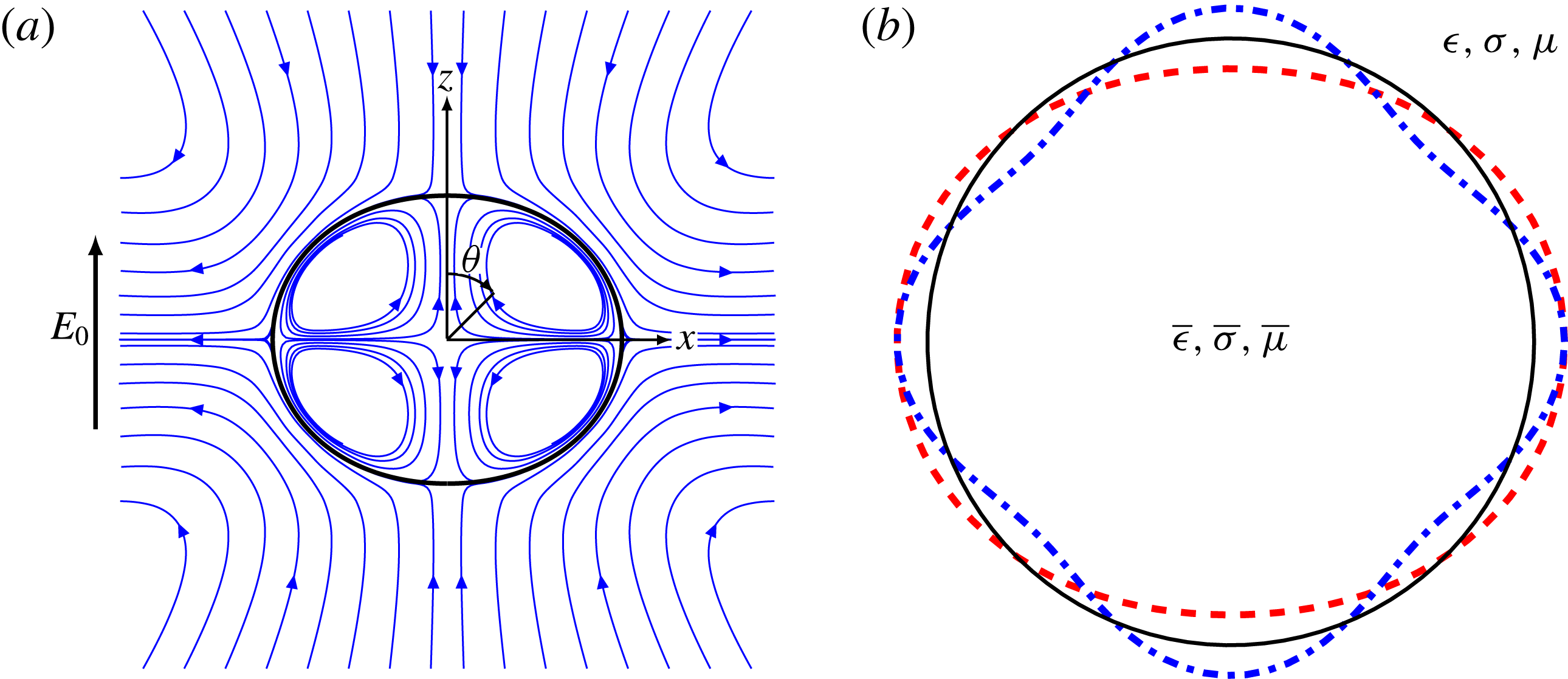
We analyse the deformation of a neutrally buoyant liquid drop suspended in another liquid and subject to a uniform electric field
 $\boldsymbol{E}_{0}=E_{0}\hat{\boldsymbol{e}}_{z}$
, as shown in figure 1. The drop, with undeformed radius
 $a$
, is assumed to carry no net charge. Both liquids are Newtonian and are treated as leaky dielectrics with constant material properties. The dielectric permittivity, electric conductivity, and dynamic viscosity of the carrying liquid are denoted by (
 $\unicode[STIX]{x1D716}$
,
 $\unicode[STIX]{x1D70E}$
,
 $\unicode[STIX]{x1D707}$
), respectively, whereas those of the drop are denoted by (
 $\bar{\unicode[STIX]{x1D716}}$
,
 $\bar{\unicode[STIX]{x1D70E}}$
,
 $\bar{\unicode[STIX]{x1D707}}$
). The interface
 $S$
between the two liquids has uniform surface tension
 $\unicode[STIX]{x1D6FE}$
and outward unit normal
 $\boldsymbol{n}$
.
Problem definition: a liquid drop is placed in a uniform electric field
 $\boldsymbol{E}_{0}$
. (
 $a$
) Spherical coordinates
 $(r,\unicode[STIX]{x1D703})$
used in axisymmetric geometry. Streamlines show the direction of the flow at steady state in the case of an oblately deformed drop. (
 $b$
) Drop shape expanded on the basis of spherical harmonics. The full line corresponds to the spherical shape, while the dashed line and dash-dotted line correspond to second-order
 ${\mathcal{L}}_{2}$
and fourth-order
 ${\mathcal{L}}_{4}$
deformation modes, respectively.

Following the Melcher–Taylor leaky dielectric model (Melcher & Taylor Reference Melcher and Taylor1969), we assume that any net charge in the system is concentrated at the interface between the two liquids. Under this condition, the electric potentials
 $\unicode[STIX]{x1D711}$
and
 $\bar{\unicode[STIX]{x1D711}}$
outside and inside the drop both satisfy Laplace’s equation:
 $$\begin{eqnarray}\unicode[STIX]{x1D6FB}^{2}\unicode[STIX]{x1D711}=0,\quad \unicode[STIX]{x1D6FB}^{2}\bar{\unicode[STIX]{x1D711}}=0.\end{eqnarray}$$
The potential is continuous across the interface:
 $$\begin{eqnarray}\unicode[STIX]{x1D711}(\boldsymbol{x})=\bar{\unicode[STIX]{x1D711}}(\boldsymbol{x})\quad \text{for }\boldsymbol{x}\in S,\end{eqnarray}$$
and approaches the externally applied potential far away from the drop:
 $$\begin{eqnarray}\unicode[STIX]{x1D711}(\boldsymbol{x})\rightarrow \unicode[STIX]{x1D711}_{e}(\boldsymbol{x})=-\boldsymbol{E}_{0}\boldsymbol{\cdot }\boldsymbol{x}\quad \text{as }|\boldsymbol{x}|\rightarrow \infty .\end{eqnarray}$$
Due to the mismatch in material properties, a surface charge density
 $q(\boldsymbol{x})$
develops at the interface between the two liquids as the drop polarizes, and is given by Gauss’s law:
 $$\begin{eqnarray}q(\boldsymbol{x})=\boldsymbol{n}\boldsymbol{\cdot }\unicode[STIX]{x27E6}\unicode[STIX]{x1D716}\boldsymbol{E}(\boldsymbol{x})\unicode[STIX]{x27E7}=\unicode[STIX]{x1D716}E^{n}(\boldsymbol{x})-\bar{\unicode[STIX]{x1D716}}\bar{E}^{n}(\boldsymbol{x}),\end{eqnarray}$$
where
 $\boldsymbol{E}=-\unicode[STIX]{x1D735}\unicode[STIX]{x1D711}$
is the local electric field and
 $E^{n}=\boldsymbol{n}\boldsymbol{\cdot }\boldsymbol{E}$
its normal component. The charge density
 $q$
evolves due to two distinct mechanisms: Ohmic currents
 $\boldsymbol{j}=\unicode[STIX]{x1D70E}\boldsymbol{E}$
from the bulk, and surface charge convection by the fluid flow with velocity
 $\boldsymbol{v}$
along the interface. Accordingly, it satisfies the conservation equation
 $$\begin{eqnarray}\unicode[STIX]{x2202}_{t}q+\boldsymbol{n}\boldsymbol{\cdot }\unicode[STIX]{x27E6}\,\boldsymbol{j}\unicode[STIX]{x27E7}+\unicode[STIX]{x1D735}_{s}\boldsymbol{\cdot }(q\boldsymbol{v})=0,\end{eqnarray}$$
where
 $\unicode[STIX]{x1D735}_{s}\equiv (\unicode[STIX]{x1D644}-\boldsymbol{n}\boldsymbol{n})\boldsymbol{\cdot }\unicode[STIX]{x1D735}$
is the surface gradient operator. The flow velocity, which is driven by electric stresses on the interface, satisfies the Stokes equations in both liquids:
 $$\begin{eqnarray}\displaystyle \displaystyle -\unicode[STIX]{x1D707}\unicode[STIX]{x1D6FB}^{2}\boldsymbol{v}+\unicode[STIX]{x1D735}p^{H} & = & \displaystyle \mathbf{0},\quad \unicode[STIX]{x1D735}\boldsymbol{\cdot }\boldsymbol{v}=0,\end{eqnarray}$$
 $$\begin{eqnarray}\displaystyle \displaystyle -\bar{\unicode[STIX]{x1D707}}\unicode[STIX]{x1D6FB}^{2}\bar{\boldsymbol{v}}+\unicode[STIX]{x1D735}\bar{p}^{H} & = & \displaystyle \mathbf{0},\quad \unicode[STIX]{x1D735}\boldsymbol{\cdot }\bar{\boldsymbol{v}}=0,\end{eqnarray}$$
 $p^{H}$
denotes the hydrodynamic pressure in the fluid. In the absence of Marangoni effects, the jumps in electric and hydrodynamic tractions balance interfacial tension forces:
 $$\begin{eqnarray}\unicode[STIX]{x27E6}\,\boldsymbol{f}^{E}\unicode[STIX]{x27E7}+\unicode[STIX]{x27E6}\,\boldsymbol{f}^{H}\unicode[STIX]{x27E7}=\unicode[STIX]{x1D6FE}(\unicode[STIX]{x1D735}_{s}\boldsymbol{\cdot }\boldsymbol{n})\boldsymbol{n}\quad \text{for}\,\,\,\boldsymbol{x}\in S,\end{eqnarray}$$
where
 $\unicode[STIX]{x1D735}_{s}\boldsymbol{\cdot }\boldsymbol{n}$
is the total surface curvature. The jumps in tractions are expressed in terms of the Maxwell stress tensor
 $\unicode[STIX]{x1D64F}^{E}$
and hydrodynamic stress tensor
 $\unicode[STIX]{x1D64F}^{H}$
as
 $$\begin{eqnarray}\displaystyle \unicode[STIX]{x27E6}\,\boldsymbol{f}^{E}\unicode[STIX]{x27E7} & = & \displaystyle \boldsymbol{n}\boldsymbol{\cdot }\unicode[STIX]{x27E6}\unicode[STIX]{x1D64F}^{E}\unicode[STIX]{x27E7}=\boldsymbol{n}\boldsymbol{\cdot }\unicode[STIX]{x27E6}\unicode[STIX]{x1D716}(\boldsymbol{E}\boldsymbol{E}-{\textstyle \frac{1}{2}}E^{2}\unicode[STIX]{x1D644})\unicode[STIX]{x27E7},\end{eqnarray}$$
 $$\begin{eqnarray}\displaystyle \unicode[STIX]{x27E6}\,\boldsymbol{f}^{H}\unicode[STIX]{x27E7} & = & \displaystyle \boldsymbol{n}\boldsymbol{\cdot }\unicode[STIX]{x27E6}\unicode[STIX]{x1D64F}^{H}\unicode[STIX]{x27E7}=\boldsymbol{n}\boldsymbol{\cdot }\unicode[STIX]{x27E6}-p^{H}\,\unicode[STIX]{x1D644}+\unicode[STIX]{x1D707}\left(\unicode[STIX]{x1D735}\boldsymbol{v}+\unicode[STIX]{x1D735}\boldsymbol{v}^{T}\right)\unicode[STIX]{x27E7}.\end{eqnarray}$$
 $$\begin{eqnarray}\displaystyle \unicode[STIX]{x27E6}\,\boldsymbol{f}^{E}\unicode[STIX]{x27E7} & = & \displaystyle [\unicode[STIX]{x1D716}E^{n}-\bar{\unicode[STIX]{x1D716}}\bar{E}^{n}]\boldsymbol{E}^{t}+{\textstyle \frac{1}{2}}[\unicode[STIX]{x1D716}(E^{n2}-E^{t2})-\bar{\unicode[STIX]{x1D716}}(\bar{E}^{n2}-E^{t2})]\boldsymbol{n}\nonumber\\ \displaystyle & = & \displaystyle q\boldsymbol{E}^{t}+\unicode[STIX]{x27E6}\,p^{E}\unicode[STIX]{x27E7}\boldsymbol{n}.\end{eqnarray}$$
Here,
 $\boldsymbol{E}^{t}=(\unicode[STIX]{x1D644}-\boldsymbol{n}\boldsymbol{n})\boldsymbol{\cdot }\boldsymbol{E}$
is the tangential electric field, which is continuous across the interface. The first term on the right-hand side captures the tangential electric force arising from the action of the tangential field on the interfacial charge. The second term captures normal electric stresses and can be interpreted as a jump in an electric pressure
 $p^{E}$
(Lac & Homsy Reference Lac and Homsy2007).
In the remainder of the paper, we scale all lengths by the radius
 $a$
and times by the Maxwell–Wagner relaxation time
 $\unicode[STIX]{x1D70F}_{MW}$
, which is the characteristic time scale for polarization of the drop:
 $$\begin{eqnarray}\unicode[STIX]{x1D70F}_{MW}=\frac{\bar{\unicode[STIX]{x1D716}}+2\unicode[STIX]{x1D716}}{\bar{\unicode[STIX]{x1D70E}}+2\unicode[STIX]{x1D70E}}.\end{eqnarray}$$
Electric and hydrodynamic stresses are non-dimensionalized by
 $\unicode[STIX]{x1D716}E_{0}^{2}$
and
 $\unicode[STIX]{x1D707}/\unicode[STIX]{x1D70F}_{MW}$
, respectively. Upon scaling of the governing equations, five dimensionless parameters emerge, three of which are ratios of material properties:
 $$\begin{eqnarray}Q=\frac{\bar{\unicode[STIX]{x1D716}}}{\unicode[STIX]{x1D716}},\quad R=\frac{\unicode[STIX]{x1D70E}}{\bar{\unicode[STIX]{x1D70E}}},\quad \unicode[STIX]{x1D706}=\frac{\bar{\unicode[STIX]{x1D707}}}{\unicode[STIX]{x1D707}}.\end{eqnarray}$$
The product
 $RQ$
, which sets the type of deformation and direction of the flow at steady state (Lac & Homsy Reference Lac and Homsy2007), can also be interpreted as the ratio of the inner and outer charge relaxation times:
 $$\begin{eqnarray}RQ=\frac{\bar{\unicode[STIX]{x1D70F}}}{\unicode[STIX]{x1D70F}}\quad \text{where }\unicode[STIX]{x1D70F}=\frac{\unicode[STIX]{x1D716}}{\unicode[STIX]{x1D70E}},\bar{\unicode[STIX]{x1D70F}}=\frac{\bar{\unicode[STIX]{x1D716}}}{\bar{\unicode[STIX]{x1D70E}}}.\end{eqnarray}$$
The two remaining dimensionless parameters are chosen as the electric capillary number
 $Ca_{E}$
, denoting the ratio of electric to capillary forces, and the Mason number
 $Ma$
, denoting the ratio of viscous to electric stresses:
 $$\begin{eqnarray}Ca_{E}=\frac{a\unicode[STIX]{x1D716}E_{0}^{2}}{\unicode[STIX]{x1D6FE}},\quad Ma=\frac{\unicode[STIX]{x1D707}}{\unicode[STIX]{x1D716}\unicode[STIX]{x1D70F}_{MW}E_{0}^{2}}.\end{eqnarray}$$
The Mason number is directly related to the electric Reynolds number
 $Re_{E}$
(Melcher & Taylor Reference Melcher and Taylor1969; Salipante & Vlahovska Reference Salipante and Vlahovska2010; Lanauze et al.
Reference Lanauze, Walker and Khair2015) as:
 $$\begin{eqnarray}Re_{E}=\frac{1}{Ma}\frac{1+2R}{R(Q+2)}.\end{eqnarray}$$
It is instructive to note that the definition of the Mason number is based on the suspending fluid viscosity. In most cases the strength of charge convection is inversely proportional to the Mason number; however, for drop–fluid systems with high viscosity ratios (
 $\unicode[STIX]{x1D706}\gg 1$
), the strength of charge convection can be weak even for small values of
 $Ma$
.
3 Problem solution by domain perturbation
We solve the governing equations for axisymmetric shapes in the limit of small deformations (Taylor Reference Taylor1966; Ajayi Reference Ajayi1978; Rallison Reference Rallison1984), which occurs when surface tension is strong enough to overcome deformations due to electric stresses. This corresponds to the limit of
 $Ca_{E}\rightarrow 0$
, and allows us to use an asymptotic approach in which we expand the drop deformation about the spherical shape and all the field variables in a small shape parameter
 $\unicode[STIX]{x1D6FF}$
, whose relation with
 $Ca_{E}$
we explain later. We employ the domain perturbation technique pioneered by Joseph (Reference Joseph1967), which was also used in a number of previous models for the dynamics of charged drops (Tsamopoulos, Akylas & Brown Reference Tsamopoulos, Akylas and Brown1985; Pelekasis, Tsamopoulos & Manolis Reference Pelekasis, Tsamopoulos and Manolis1990).
3.1 Shape parametrization and expansion
In axisymmetric geometry, we parametrize the drop shape as a curve
 $\unicode[STIX]{x1D709}(r,\unicode[STIX]{x1D702})=0$
, where
 $r=|\boldsymbol{x}|$
is the distance from the drop centre and
 $\unicode[STIX]{x1D702}=\cos \unicode[STIX]{x1D703}$
is the cosine of the polar angle
 $\unicode[STIX]{x1D703}\in [0,\unicode[STIX]{x03C0}]$
measured from the field direction. For small deviations from sphericity, the drop shape is expanded on the basis of spherical harmonics as
 $$\begin{eqnarray}\unicode[STIX]{x1D709}(r,\unicode[STIX]{x1D702})=r-(1+\unicode[STIX]{x1D6FF}f_{1}+\unicode[STIX]{x1D6FF}^{2}f_{2})+O(\unicode[STIX]{x1D6FF}^{3}).\end{eqnarray}$$
The first- and second-order shape functions are linear combinations of Legendre polynomials
 ${\mathcal{L}}_{n}$
of order
 $n$
:
 $$\begin{eqnarray}\displaystyle f_{1} & = & \displaystyle f_{12}{\mathcal{L}}_{2}(\unicode[STIX]{x1D702}),\end{eqnarray}$$
 $$\begin{eqnarray}\displaystyle f_{2} & = & \displaystyle f_{20}+f_{22}{\mathcal{L}}_{2}(\unicode[STIX]{x1D702})+f_{24}{\mathcal{L}}_{4}(\unicode[STIX]{x1D702}),\end{eqnarray}$$
 ${\mathcal{L}}_{2}$
and
 ${\mathcal{L}}_{4}$
are illustrated in figure 1(
 $b$
). We note the orthogonality condition
 $$\begin{eqnarray}\displaystyle \int _{0}^{\unicode[STIX]{x03C0}}{\mathcal{L}}_{i}(\unicode[STIX]{x1D702}){\mathcal{L}}_{j}(\unicode[STIX]{x1D702})\sin \unicode[STIX]{x1D703}\,\text{d}\unicode[STIX]{x1D703}=\frac{2}{2i+1}\unicode[STIX]{x1D6FF}_{ij}, & & \displaystyle\end{eqnarray}$$
where
 $\unicode[STIX]{x1D6FF}_{ij}$
denotes the Kronecker delta, which will become useful later. The choice of Legendre functions in (3.2a
)–(3.2b
) is a consequence of the quadratic nature of the Maxwell electric stresses acting on the fluid–drop interface, which in a uniform electric field only excite shape modes of order
 $2^{n}$
(
 $n\in \mathbb{Z}^{+}$
). In (3.2a
)–(3.2b
) and in the rest of the paper, pairs of indices in coefficients of the form
 $f_{ij}$
refer to the order
 $i$
in the small-deformation expansion and to the order
 $j$
of the Legendre polynomial they multiply, respectively. In (3.2b
), the constant term
 $f_{20}$
is added to the second-order shape function
 $f_{2}$
to negate the perturbation in the drop volume due to the first-order shape function
 $f_{1}$
:
 $$\begin{eqnarray}2\unicode[STIX]{x03C0}\int _{0}^{\unicode[STIX]{x03C0}}\int _{0}^{r}\unicode[STIX]{x1D70C}^{2}\sin \unicode[STIX]{x1D703}\hspace{2.22198pt}\text{d}\unicode[STIX]{x1D70C}\hspace{2.22198pt}\text{d}\unicode[STIX]{x1D703}=\frac{4\unicode[STIX]{x03C0}}{3}+4\unicode[STIX]{x03C0}\unicode[STIX]{x1D6FF}^{2}\left(\frac{f_{12}^{2}}{5}+f_{20}\right)+O(\unicode[STIX]{x1D6FF}^{3}).\end{eqnarray}$$
Requiring terms of order
 $\unicode[STIX]{x1D6FF}^{2}$
to vanish, we get
 $f_{20}=-f_{12}^{2}/5$
. The outward unit normal, tangent vector and curvature of the interface are also obtained as (Ajayi Reference Ajayi1978)
 $$\begin{eqnarray}\displaystyle & \boldsymbol{n}=\hat{\boldsymbol{e}}_{r}-\unicode[STIX]{x1D6FF}\,\unicode[STIX]{x2202}_{\unicode[STIX]{x1D703}}f_{1}\,\hat{\boldsymbol{e}}_{\unicode[STIX]{x1D703}}+O(\unicode[STIX]{x1D6FF}^{2}),\quad \boldsymbol{t}=\hat{\boldsymbol{e}}_{\unicode[STIX]{x1D703}}+\unicode[STIX]{x1D6FF}\,\unicode[STIX]{x2202}_{\unicode[STIX]{x1D703}}f_{1}\,\hat{\boldsymbol{e}}_{r}+O(\unicode[STIX]{x1D6FF}^{2}), & \displaystyle\end{eqnarray}$$
 $$\begin{eqnarray}\displaystyle \unicode[STIX]{x1D735}_{s}\boldsymbol{\cdot }\boldsymbol{n}=2-\unicode[STIX]{x1D6FF}L[f_{1}]-\unicode[STIX]{x1D6FF}^{2}\{L[f_{2}]-2f_{1}(L[f_{1}]-f_{1})\}+O(\unicode[STIX]{x1D6FF}^{3}), & & \displaystyle\end{eqnarray}$$
 $L$
is defined as
 $L[f]=\unicode[STIX]{x2202}_{\unicode[STIX]{x1D702}}\{(1-\unicode[STIX]{x1D702}^{2})\unicode[STIX]{x2202}_{\unicode[STIX]{x1D702}}f\}+2f$
.
Using the above parametrization, the normal and tangential components of any vector
 $\boldsymbol{v}$
and second-order tensor
 $\unicode[STIX]{x1D64F}$
on the drop surface are related to their components in spherical coordinates by
 $$\begin{eqnarray}\displaystyle v^{n} & = & \displaystyle v_{0}^{r}+\unicode[STIX]{x1D6FF}(v_{1}^{r}+f_{1}\unicode[STIX]{x2202}_{r}v_{0}^{r}-\unicode[STIX]{x2202}_{\unicode[STIX]{x1D703}}f_{1}v_{0}^{\unicode[STIX]{x1D703}})+O(\unicode[STIX]{x1D6FF}^{2}),\end{eqnarray}$$
 $$\begin{eqnarray}\displaystyle v^{t} & = & \displaystyle v_{0}^{\unicode[STIX]{x1D703}}+\unicode[STIX]{x1D6FF}(v_{1}^{\unicode[STIX]{x1D703}}+f_{1}\unicode[STIX]{x2202}_{r}v_{0}^{\unicode[STIX]{x1D703}}+\unicode[STIX]{x2202}_{\unicode[STIX]{x1D703}}f_{1}v_{0}^{r})+O(\unicode[STIX]{x1D6FF}^{2}),\end{eqnarray}$$
 $$\begin{eqnarray}\displaystyle T^{nn} & = & \displaystyle T_{0}^{rr}+\unicode[STIX]{x1D6FF}(T_{1}^{rr}+f_{1}\unicode[STIX]{x2202}_{r}T_{0}^{rr}-2\unicode[STIX]{x2202}_{\unicode[STIX]{x1D703}}f_{1}T_{0}^{r\unicode[STIX]{x1D703}})+O(\unicode[STIX]{x1D6FF}^{2}),\end{eqnarray}$$
 $$\begin{eqnarray}\displaystyle T^{nt} & = & \displaystyle T_{0}^{r\unicode[STIX]{x1D703}}+\unicode[STIX]{x1D6FF}[T_{1}^{r\unicode[STIX]{x1D703}}+f_{1}\unicode[STIX]{x2202}_{r}T_{0}^{r\unicode[STIX]{x1D703}}+\unicode[STIX]{x2202}_{\unicode[STIX]{x1D703}}f_{1}(T_{0}^{rr}-T_{0}^{\unicode[STIX]{x1D703}\unicode[STIX]{x1D703}})]+O(\unicode[STIX]{x1D6FF}^{2}),\end{eqnarray}$$
 $r=1$
. These expressions will be useful below in determining the electric field, fluid velocity and stress distributions on the drop surface.
3.2 Electric problem
3.2.1 Spherical harmonic expansion
We first present the solution to the electric problem, which consists in solving (2.1)–(2.3) asymptotically. The electric potential outside and inside the drop can be expanded in powers of
 $\unicode[STIX]{x1D6FF}$
as
 $$\begin{eqnarray}\displaystyle \unicode[STIX]{x1D711} & = & \displaystyle \unicode[STIX]{x1D711}_{e}(r,\unicode[STIX]{x1D703})+\unicode[STIX]{x1D711}_{0}(r,\unicode[STIX]{x1D703})+\unicode[STIX]{x1D6FF}\unicode[STIX]{x1D711}_{1}(r,\unicode[STIX]{x1D703})+O(\unicode[STIX]{x1D6FF}^{2}),\end{eqnarray}$$
 $$\begin{eqnarray}\displaystyle \bar{\unicode[STIX]{x1D711}} & = & \displaystyle \unicode[STIX]{x1D711}_{e}(r,\unicode[STIX]{x1D703})+\bar{\unicode[STIX]{x1D711}}_{0}(r,\unicode[STIX]{x1D703})+\unicode[STIX]{x1D6FF}\bar{\unicode[STIX]{x1D711}}_{1}(r,\unicode[STIX]{x1D703})+O(\unicode[STIX]{x1D6FF}^{2}),\end{eqnarray}$$
 $r=1$
. The potential on the interface is first expanded in the neighbourhood of
 $r=1$
using Taylor series:
 $$\begin{eqnarray}\displaystyle \unicode[STIX]{x1D711} & = & \displaystyle \unicode[STIX]{x1D711}_{e}+\unicode[STIX]{x1D711}_{0}+\unicode[STIX]{x1D6FF}\left[\unicode[STIX]{x1D711}_{1}+f_{1}\unicode[STIX]{x2202}_{r}(\unicode[STIX]{x1D711}_{e}+\unicode[STIX]{x1D711}_{0})\right]+O(\unicode[STIX]{x1D6FF}^{2}),\end{eqnarray}$$
 $$\begin{eqnarray}\displaystyle \bar{\unicode[STIX]{x1D711}} & = & \displaystyle \bar{\unicode[STIX]{x1D711}}_{e}+\bar{\unicode[STIX]{x1D711}}_{0}+\unicode[STIX]{x1D6FF}\left[\bar{\unicode[STIX]{x1D711}}_{1}+f_{1}\unicode[STIX]{x2202}_{r}(\unicode[STIX]{x1D711}_{e}+\bar{\unicode[STIX]{x1D711}}_{0})\right]+O(\unicode[STIX]{x1D6FF}^{2}).\end{eqnarray}$$
 $\unicode[STIX]{x1D6FF}$
provides two boundary conditions at
 $r=1$
:
 $$\begin{eqnarray}\displaystyle \unicode[STIX]{x1D711}_{0} & = & \displaystyle \bar{\unicode[STIX]{x1D711}}_{0},\end{eqnarray}$$
 $$\begin{eqnarray}\displaystyle \unicode[STIX]{x1D711}_{1}+f_{1}\unicode[STIX]{x2202}_{r}(\unicode[STIX]{x1D711}_{e}+\unicode[STIX]{x1D711}_{0}) & = & \displaystyle \bar{\unicode[STIX]{x1D711}}_{1}+f_{1}\unicode[STIX]{x2202}_{r}(\unicode[STIX]{x1D711}_{e}+\bar{\unicode[STIX]{x1D711}}_{0}).\end{eqnarray}$$
 $P_{01}$
,
 $\bar{P}_{01}$
:
 $$\begin{eqnarray}\displaystyle \unicode[STIX]{x1D711}_{0} & = & \displaystyle P_{01}r^{-2}{\mathcal{L}}_{1}(\unicode[STIX]{x1D702}),\end{eqnarray}$$
 $$\begin{eqnarray}\displaystyle \bar{\unicode[STIX]{x1D711}}_{0} & = & \displaystyle \bar{P}_{01}r{\mathcal{L}}_{1}(\unicode[STIX]{x1D702}),\end{eqnarray}$$
 $\bar{P}_{01}=P_{01}$
to satisfy (3.9a
); solving for
 $P_{01}$
will require application of the charge conservation (2.5) as detailed below. After substitution into (3.9b
), we obtain a new first-order boundary condition:
 $$\begin{eqnarray}\unicode[STIX]{x1D711}_{1}-\bar{\unicode[STIX]{x1D711}}_{1}=3f_{1}P_{01}{\mathcal{L}}_{1}(\unicode[STIX]{x1D702})=3f_{12}P_{01}{\mathcal{L}}_{1}(\unicode[STIX]{x1D702}){\mathcal{L}}_{2}(\unicode[STIX]{x1D702})={\textstyle \frac{3}{5}}f_{12}P_{01}[2{\mathcal{L}}_{1}(\unicode[STIX]{x1D702})+3{\mathcal{L}}_{3}(\unicode[STIX]{x1D702})].\end{eqnarray}$$
The order of the polynomials appearing on the right-hand side suggests representing the first-order potentials in terms of both dipoles
 $P_{11}$
,
 $\bar{P}_{11}$
and octupoles
 $P_{13}$
,
 $\bar{P}_{13}$
:
 $$\begin{eqnarray}\displaystyle \unicode[STIX]{x1D711}_{1} & = & \displaystyle P_{11}r^{-2}{\mathcal{L}}_{1}(\unicode[STIX]{x1D702})+P_{13}r^{-4}{\mathcal{L}}_{3}(\unicode[STIX]{x1D702}),\end{eqnarray}$$
 $$\begin{eqnarray}\displaystyle \bar{\unicode[STIX]{x1D711}}_{1} & = & \displaystyle \bar{P}_{11}r{\mathcal{L}}_{1}(\unicode[STIX]{x1D702})+\bar{P}_{13}r^{3}{\mathcal{L}}_{3}(\unicode[STIX]{x1D702}),\end{eqnarray}$$
 $$\begin{eqnarray}\bar{P}_{11}=P_{11}-{\textstyle \frac{6}{5}}f_{12}P_{01},\quad \bar{P}_{13}=P_{13}-{\textstyle \frac{9}{5}}f_{12}P_{01}.\end{eqnarray}$$
Having determined the electric potential, we can also obtain asymptotic expressions for the normal and tangential electric fields
 $E^{n}=-\boldsymbol{n}\boldsymbol{\cdot }\unicode[STIX]{x1D735}\unicode[STIX]{x1D711}$
and
 $E^{t}=-\boldsymbol{t}\boldsymbol{\cdot }\unicode[STIX]{x1D735}\unicode[STIX]{x1D711}$
on the drop surface. Applying (3.6a
), we find
 $$\begin{eqnarray}E^{n}=E_{0}^{n}+\unicode[STIX]{x1D6FF}E_{1}^{n}+O(\unicode[STIX]{x1D6FF}^{2})=E_{01}^{n}{\mathcal{L}}_{1}(\unicode[STIX]{x1D702})+\unicode[STIX]{x1D6FF}[E_{11}^{n}{\mathcal{L}}_{1}(\unicode[STIX]{x1D702})+E_{13}^{n}{\mathcal{L}}_{3}(\unicode[STIX]{x1D702})]+O(\unicode[STIX]{x1D6FF}^{2}),\end{eqnarray}$$
with a similar expansion for
 $\bar{E}^{n}$
. Finally, the expansion for the tangential electric field, which is continuous across the interface, is obtained using (3.6b
) as
 $$\begin{eqnarray}E^{t}=E_{0}^{t}+\unicode[STIX]{x1D6FF}E_{1}^{t}+O(\unicode[STIX]{x1D6FF}^{2})=E_{00}^{t}\sin \unicode[STIX]{x1D703}+\unicode[STIX]{x1D6FF}[E_{10}^{t}+E_{12}^{t}{\mathcal{L}}_{2}(\unicode[STIX]{x1D702})]\sin \unicode[STIX]{x1D703}+O(\unicode[STIX]{x1D6FF}^{2}).\end{eqnarray}$$
The detailed expressions for the coefficients appearing in (3.14)–(3.15) are provided in appendix A.
3.2.2 Charge conservation and moment equations
To complete the solution of the electric problem, equations must be derived for the moments
 $P_{01}$
,
 $P_{11}$
and
 $P_{13}$
, which are time-dependent. These can be obtained as ordinary differential equations by application of the charge conservation (2.5). First, we expand the charge density in powers of
 $\unicode[STIX]{x1D6FF}$
as
 $$\begin{eqnarray}q=q_{0}+\unicode[STIX]{x1D6FF}q_{1}+O(\unicode[STIX]{x1D6FF}^{2})=q_{01}{\mathcal{L}}_{1}(\unicode[STIX]{x1D702})+\unicode[STIX]{x1D6FF}[q_{11}{\mathcal{L}}_{1}(\unicode[STIX]{x1D702})+q_{13}{\mathcal{L}}_{3}(\unicode[STIX]{x1D702})]+O(\unicode[STIX]{x1D6FF}^{2}).\end{eqnarray}$$
Similarly, we expand the jump in Ohmic currents
 $\boldsymbol{n}\boldsymbol{\cdot }\unicode[STIX]{x27E6}\,\boldsymbol{j}\unicode[STIX]{x27E7}=\unicode[STIX]{x27E6}\,j\unicode[STIX]{x27E7}^{n}$
, scaled here by
 $\bar{\unicode[STIX]{x1D70E}}E_{0}$
, as
 $$\begin{eqnarray}\unicode[STIX]{x27E6}\,j\unicode[STIX]{x27E7}^{n}=\unicode[STIX]{x27E6}\,j\unicode[STIX]{x27E7}_{0}^{n}+\unicode[STIX]{x1D6FF}\unicode[STIX]{x27E6}\,j\unicode[STIX]{x27E7}_{1}^{n}+O(\unicode[STIX]{x1D6FF}^{2})=\unicode[STIX]{x27E6}\,j\unicode[STIX]{x27E7}_{01}^{n}{\mathcal{L}}_{1}(\unicode[STIX]{x1D702})+\unicode[STIX]{x1D6FF}\{\unicode[STIX]{x27E6}\,j\unicode[STIX]{x27E7}_{11}^{n}{\mathcal{L}}_{1}(\unicode[STIX]{x1D702})+\unicode[STIX]{x27E6}\,j\unicode[STIX]{x27E7}_{13}^{n}{\mathcal{L}}_{3}(\unicode[STIX]{x1D702})\}+O(\unicode[STIX]{x1D6FF}^{2}).\end{eqnarray}$$
Expansion coefficients for both
 $q$
and
 $\unicode[STIX]{x27E6}\,j\unicode[STIX]{x27E7}^{n}$
are provided in appendix A. Finally, we formally expand the charge convection term in (2.5) as
 $$\begin{eqnarray}\displaystyle \unicode[STIX]{x1D735}_{s}\boldsymbol{\cdot }(q\boldsymbol{v}) & = & \displaystyle [\unicode[STIX]{x1D735}_{s}\boldsymbol{\cdot }(q\boldsymbol{v})]_{0}+\unicode[STIX]{x1D6FF}[\unicode[STIX]{x1D735}_{s}\boldsymbol{\cdot }(q\boldsymbol{v})]_{1}+O(\unicode[STIX]{x1D6FF}^{2}),\nonumber\\ \displaystyle & = & \displaystyle [\unicode[STIX]{x1D735}_{s}\boldsymbol{\cdot }(q\boldsymbol{v})]_{01}{\mathcal{L}}_{1}(\unicode[STIX]{x1D702})+\unicode[STIX]{x1D6FF}\{[\unicode[STIX]{x1D735}_{s}\boldsymbol{\cdot }(q\boldsymbol{v})]_{11}{\mathcal{L}}_{1}(\unicode[STIX]{x1D702})+[\unicode[STIX]{x1D735}_{s}\boldsymbol{\cdot }(q\boldsymbol{v})]_{13}{\mathcal{L}}_{3}(\unicode[STIX]{x1D702})\}+O(\unicode[STIX]{x1D6FF}^{2}),\nonumber\\ \displaystyle & & \displaystyle\end{eqnarray}$$
where we have introduced the Legendre coefficients
 $$\begin{eqnarray}\displaystyle [\unicode[STIX]{x1D735}_{s}\boldsymbol{\cdot }(q\boldsymbol{v})]_{ij}=\frac{2j+1}{2}\int _{0}^{\unicode[STIX]{x03C0}}[\unicode[STIX]{x1D735}_{s}\boldsymbol{\cdot }(q\boldsymbol{v})]_{i}{\mathcal{L}}_{j}(\unicode[STIX]{x1D702})\sin \unicode[STIX]{x1D703}\,\text{d}\unicode[STIX]{x1D703}. & & \displaystyle\end{eqnarray}$$
Detailed expressions for these coefficients require knowledge of the interfacial velocity
 $\boldsymbol{v}$
, whose calculation is presented in § 3.3. Note that the zeroth-order charge convection term arising from the nonlinear product of the charge density
 $q_{0}$
and interfacial velocity
 $\boldsymbol{v}_{0}$
also involves an additional term of the form
 $[\unicode[STIX]{x1D735}_{s}\boldsymbol{\cdot }(q\boldsymbol{v})]_{03}{\mathcal{L}}_{3}(\unicode[STIX]{x1D702})$
, which has been neglected here. To consider its effect, one would need to include a zeroth-order octupole
 $P_{03}$
in (3.10), which in turn would generate charge convection terms of orders
 $1,3,5,7,\ldots ,$
thus requiring additional higher-order odd multipoles. These multipoles becomes stronger with increasing electric Reynolds number or decreasing Mason number. Our theory is therefore valid in the limit of high Mason number, i.e. for drop–fluid systems in which charge convection is relatively weak.
Substituting the expansions (3.16)–(3.18) into the charge conservation (2.5), matching powers of
 $\unicode[STIX]{x1D6FF}$
, and applying orthogonality of Legendre polynomials leads to a set of relaxation equations for the charge coefficients. In dimensionless form, these read
 $$\begin{eqnarray}\dot{q}_{ij}+\frac{Q+2}{1+2R}\,\unicode[STIX]{x27E6}\,j\unicode[STIX]{x27E7}_{ij}^{n}+[\unicode[STIX]{x1D735}_{s}\boldsymbol{\cdot }(q\boldsymbol{v})]_{ij}=0,\end{eqnarray}$$
where the dot in the first term denotes differentiation with respect to time. If we further express
 $q_{ij}$
and
 $\unicode[STIX]{x27E6}\,j\unicode[STIX]{x27E7}_{ij}^{n}$
in terms of
 $P_{01}$
,
 $P_{11}$
and
 $P_{13}$
using (A 2) and (A 3), we arrive at a set of hierarchical differential equations for the dipole and octupole moments:
 $$\begin{eqnarray}\displaystyle {\dot{P}}_{01}+P_{01}=\frac{1-R}{1+2R}-\frac{1}{Q+2}[\unicode[STIX]{x1D735}_{s}\boldsymbol{\cdot }(q\boldsymbol{v})]_{01}, & & \displaystyle\end{eqnarray}$$
 $$\begin{eqnarray}\displaystyle {\dot{P}}_{11}+P_{11} & = & \displaystyle \frac{\text{d}}{\text{d}t}\left[\frac{6}{5}f_{12}\left(P_{01}\frac{1+2Q}{2+Q}+\frac{1-Q}{2+Q}\right)\right]+\frac{6}{5}f_{12}\left(P_{01}\frac{R+2}{2R+1}-\frac{1-R}{2R+1}\right)\nonumber\\ \displaystyle & & \displaystyle -\,\frac{1}{Q+2}[\unicode[STIX]{x1D735}_{s}\boldsymbol{\cdot }(q\boldsymbol{v})]_{11},\end{eqnarray}$$
 $$\begin{eqnarray}\displaystyle {\dot{P}}_{13}+\frac{Q+2}{3Q+4}\frac{4R+3}{2R+1}P_{13} & = & \displaystyle \frac{\text{d}}{\text{d}t}\left[\frac{6}{5}f_{12}\left(P_{01}\frac{8+7Q}{8+6Q}-\frac{1-Q}{4+3Q}\right)\right]\nonumber\\ \displaystyle & & \displaystyle +\,\frac{6}{5}f_{12}\frac{Q+2}{3Q+4}\left(P_{01}\frac{8R+7}{4R+2}+\frac{1-R}{2R+1}\right)\nonumber\\ \displaystyle & & \displaystyle -\,\frac{1}{3Q+4}[\unicode[STIX]{x1D735}_{s}\boldsymbol{\cdot }(q\boldsymbol{v})]_{13}.\end{eqnarray}$$
These coupled ordinary differential equations constitute the main result of this section. The external forcing in these equations is encapsulated in the first term on the right-hand side of (3.21), which describes the effect of the applied electric field on the leading-order dipole moment. It is also clear from (3.21) that charge convection cannot be neglected even at zeroth order, as was previously done in the theories of Shutov (Reference Shutov2002) and Shkadov & Shutov (Reference Shkadov and Shutov2002). Solving (3.21)–(3.23) requires the Legendre coefficients of the charge convection term as well as the first-order shape coefficient
 $f_{12}$
. These unknowns will be determined below after we solve for the fluid flow, which affects both interfacial charge convection and droplet deformation.
3.3 Flow problem: streamfunction formulation
We now turn to the calculation of the fluid flow outside and inside the drop. Upon application of the field, electric stresses develop at the interface, leading to deformations and flow. Since the flow is axisymmetric, we use a Stokes streamfunction
 $\unicode[STIX]{x1D6F9}(r,\unicode[STIX]{x1D703})$
to determine the fluid velocity, which has components
 $$\begin{eqnarray}v^{r}=\frac{1}{r^{2}\sin \unicode[STIX]{x1D703}}\unicode[STIX]{x2202}_{\unicode[STIX]{x1D703}}\unicode[STIX]{x1D6F9},\quad v^{\unicode[STIX]{x1D703}}=-\frac{1}{r\sin \unicode[STIX]{x1D703}}\unicode[STIX]{x2202}_{r}\unicode[STIX]{x1D6F9},\end{eqnarray}$$
in spherical coordinates. The streamfunction satisfies the biharmonic equation
 $\unicode[STIX]{x1D6FB}^{4}\unicode[STIX]{x1D6F9}=0$
, the general solutions to which outside and inside the drop are (Kim & Karrila Reference Kim and Karrila2013):
 $$\begin{eqnarray}\displaystyle \unicode[STIX]{x1D6F9}=\mathop{\sum }_{n=2}^{\infty }(A_{n}r^{-n+1}+B_{n}r^{-n+3}){\mathcal{G}}_{n}(\unicode[STIX]{x1D702}),\quad \bar{\unicode[STIX]{x1D6F9}}=\mathop{\sum }_{n=2}^{\infty }(\bar{A}_{n}r^{n}+\bar{B}_{n}r^{n+2}){\mathcal{G}}_{n}(\unicode[STIX]{x1D702}), & & \displaystyle\end{eqnarray}$$
where
 ${\mathcal{G}}_{n}(\unicode[STIX]{x1D702})$
are Gegenbauer functions of degree
 $-1/2$
of the first kind (Abramowitz & Stegun Reference Abramowitz and Stegun1972). They are related to Legendre polynomials and are regular everywhere in
 $-1\leqslant \unicode[STIX]{x1D702}\leqslant 1$
:
 $$\begin{eqnarray}\displaystyle {\mathcal{G}}_{n}(\unicode[STIX]{x1D702})=\frac{{\mathcal{L}}_{n-2}(\unicode[STIX]{x1D702})-{\mathcal{L}}_{n}(\unicode[STIX]{x1D702})}{2n-1},~~~n\geqslant 2. & & \displaystyle\end{eqnarray}$$
The first two functions are defined as
 ${\mathcal{G}}_{0}(\unicode[STIX]{x1D702})=1$
and
 ${\mathcal{G}}_{1}(\unicode[STIX]{x1D702})=-\unicode[STIX]{x1D702}$
, and we also note the property:
 ${\mathcal{G}}_{n}^{\prime }(\unicode[STIX]{x1D702})=-{\mathcal{L}}_{n-1}(\unicode[STIX]{x1D702})$
.
Following the same methodology as for the electric problem, we seek solutions as expansions in powers of
 $\unicode[STIX]{x1D6FF}$
. As will become evident in § 3.5 when performing the stress balance on the interface, the zeroth- and first-order electric stresses acting on the interface at most induce fluid motions of the form
 $$\begin{eqnarray}\displaystyle \unicode[STIX]{x1D6F9} & = & \displaystyle \unicode[STIX]{x1D6F9}_{03}{\mathcal{G}}_{3}(\unicode[STIX]{x1D702})+\unicode[STIX]{x1D6FF}[\unicode[STIX]{x1D6F9}_{13}{\mathcal{G}}_{3}(\unicode[STIX]{x1D702})+\unicode[STIX]{x1D6F9}_{15}{\mathcal{G}}_{5}(\unicode[STIX]{x1D702})]+O(\unicode[STIX]{x1D6FF}^{2}),\end{eqnarray}$$
 $$\begin{eqnarray}\displaystyle \bar{\unicode[STIX]{x1D6F9}} & = & \displaystyle \bar{\unicode[STIX]{x1D6F9}}_{03}{\mathcal{G}}_{3}(\unicode[STIX]{x1D702})+\unicode[STIX]{x1D6FF}[\bar{\unicode[STIX]{x1D6F9}}_{13}{\mathcal{G}}_{3}(\unicode[STIX]{x1D702})+\bar{\unicode[STIX]{x1D6F9}}_{15}{\mathcal{G}}_{5}(\unicode[STIX]{x1D702})]+O(\unicode[STIX]{x1D6FF}^{2}),\end{eqnarray}$$
 $$\begin{eqnarray}\displaystyle \unicode[STIX]{x1D6F9}_{03}=A_{03}r^{-2}+B_{03},\quad \bar{\unicode[STIX]{x1D6F9}}_{03}=\bar{A}_{03}r^{3}+\bar{B}_{03}r^{5}, & & \displaystyle\end{eqnarray}$$
 $$\begin{eqnarray}\displaystyle \unicode[STIX]{x1D6F9}_{13}=A_{13}r^{-2}+B_{13},\quad \bar{\unicode[STIX]{x1D6F9}}_{13}=\bar{A}_{13}r^{3}+\bar{B}_{13}r^{5}, & & \displaystyle\end{eqnarray}$$
 $$\begin{eqnarray}\displaystyle \unicode[STIX]{x1D6F9}_{15}=A_{15}r^{-4}+B_{15}r^{-2},\quad \bar{\unicode[STIX]{x1D6F9}}_{15}=\bar{A}_{15}r^{5}+\bar{B}_{15}r^{7}. & & \displaystyle\end{eqnarray}$$
3.4 Kinematic boundary condition
The kinematic boundary condition relates the shape deformation to the fluid velocity so as to satisfy the no-slip and no-penetration boundary conditions at the interface. The streamfunction
 $\unicode[STIX]{x1D6F9}$
can be used to determine the normal and tangential components of the fluid velocity on the drop surface, which are obtained by combining (3.6a
)–(3.6b
) and (3.24) as
 $$\begin{eqnarray}\displaystyle v^{n} & = & \displaystyle v_{02}^{n}{\mathcal{L}}_{2}(\unicode[STIX]{x1D702})+\unicode[STIX]{x1D6FF}[v_{10}^{n}+v_{12}^{n}{\mathcal{L}}_{2}(\unicode[STIX]{x1D702})+v_{14}^{n}{\mathcal{L}}_{4}(\unicode[STIX]{x1D702})]+O(\unicode[STIX]{x1D6FF}^{2}),\end{eqnarray}$$
 $$\begin{eqnarray}\displaystyle \bar{v}^{n} & = & \displaystyle \bar{v}_{02}^{n}{\mathcal{L}}_{2}(\unicode[STIX]{x1D702})+\unicode[STIX]{x1D6FF}[\bar{v}_{10}^{n}+\bar{v}_{12}^{n}{\mathcal{L}}_{2}(\unicode[STIX]{x1D702})+\bar{v}_{14}^{n}{\mathcal{L}}_{4}(\unicode[STIX]{x1D702})]+O(\unicode[STIX]{x1D6FF}^{2}),\end{eqnarray}$$
 $$\begin{eqnarray}\displaystyle v^{t} & = & \displaystyle v_{01}^{t}{\mathcal{L}}_{1}(\unicode[STIX]{x1D702})\sin \unicode[STIX]{x1D703}+\unicode[STIX]{x1D6FF}[v_{11}^{t}{\mathcal{L}}_{1}(\unicode[STIX]{x1D702})+v_{13}^{t}{\mathcal{L}}_{3}(\unicode[STIX]{x1D702})]\sin \unicode[STIX]{x1D703}+O(\unicode[STIX]{x1D6FF}^{2}),\end{eqnarray}$$
 $$\begin{eqnarray}\displaystyle \bar{v}^{t} & = & \displaystyle \bar{v}_{01}^{t}{\mathcal{L}}_{1}(\unicode[STIX]{x1D702})\sin \unicode[STIX]{x1D703}+\unicode[STIX]{x1D6FF}[\bar{v}_{11}^{t}{\mathcal{L}}_{1}(\unicode[STIX]{x1D702})+\bar{v}_{13}^{t}{\mathcal{L}}_{3}(\unicode[STIX]{x1D702})]\sin \unicode[STIX]{x1D703}+O(\unicode[STIX]{x1D6FF}^{2}).\end{eqnarray}$$
 $v^{n}=\bar{v}^{n}=-\dot{\unicode[STIX]{x1D709}}$
, which yields the eight relations
 $$\begin{eqnarray}\displaystyle & \displaystyle v_{02}^{n}=\bar{v}_{02}^{n}=\unicode[STIX]{x1D6FF}{\dot{f}}_{12},\quad v_{10}^{n}=\bar{v}_{10}^{n}=\unicode[STIX]{x1D6FF}{\dot{f}}_{20}, & \displaystyle\end{eqnarray}$$
 $$\begin{eqnarray}\displaystyle & \displaystyle v_{12}^{n}=\bar{v}_{12}^{n}=\unicode[STIX]{x1D6FF}{\dot{f}}_{22},\quad v_{14}^{n}=\bar{v}_{14}^{n}=\unicode[STIX]{x1D6FF}{\dot{f}}_{24}. & \displaystyle\end{eqnarray}$$
Similarly, the no-slip boundary condition
 $v^{t}=\bar{v}^{t}$
dictates that
 $$\begin{eqnarray}v_{01}^{t}=\bar{v}_{01}^{t},\quad v_{11}^{t}=\bar{v}_{11}^{t},\quad v_{13}^{t}=\bar{v}_{13}^{t}.\end{eqnarray}$$
The matching of orders in (3.30) might seem surprising at first due to the presence of terms involving
 $\unicode[STIX]{x1D6FF}$
on the right-hand side. However, it is the only possible solution, as the leading-order term in
 $\dot{\unicode[STIX]{x1D709}}$
involves
 $\unicode[STIX]{x1D6FF}$
. This implies that temporal derivatives of the shape functions in fact scale as
 $\unicode[STIX]{x1D6FF}^{-1}$
, suggesting that the characteristic time scale for the shape transient is not the Maxwell–Wagner relaxation time used here for non-dimensionalization. This point will be made clearer in § 4.2.
3.5 Dynamic boundary condition
We now proceed to enforce the dynamic boundary condition of (2.7), which in dimensionless form reads
 $$\begin{eqnarray}\displaystyle \boldsymbol{n}\boldsymbol{\cdot }(\unicode[STIX]{x27E6}\boldsymbol{T}^{E}\unicode[STIX]{x27E7}+Ma\,\unicode[STIX]{x27E6}\boldsymbol{T}^{H}\unicode[STIX]{x27E7})=\frac{1}{Ca_{E}}(\unicode[STIX]{x1D735}_{s}\boldsymbol{\cdot }\boldsymbol{n})\boldsymbol{n}, & & \displaystyle\end{eqnarray}$$
and requires us to evaluate electric and hydrodynamic stresses on the interface.
3.5.1 Electric and hydrodynamic stresses
As previously shown in (2.9), the jump in electric tractions can be decomposed into tangential and normal components, both of which involve quadratic products of expansions derived above. The tangential component
 $q\boldsymbol{E}^{t}=qE^{t}\boldsymbol{t}$
is continuous and is expanded as
 $$\begin{eqnarray}qE^{t}=[qE^{t}]_{01}{\mathcal{L}}_{1}(\unicode[STIX]{x1D702})\sin \unicode[STIX]{x1D703}+\unicode[STIX]{x1D6FF}\{[qE^{t}]_{11}{\mathcal{L}}_{1}(\unicode[STIX]{x1D702})+[qE^{t}]_{13}{\mathcal{L}}_{3}(\unicode[STIX]{x1D702})\}\sin \unicode[STIX]{x1D703}+O(\unicode[STIX]{x1D6FF}^{2}).\end{eqnarray}$$
Similarly, the expansion for the jump in electric pressure in (2.9) is found to be
 $$\begin{eqnarray}\unicode[STIX]{x27E6}\,p^{E}\unicode[STIX]{x27E7}=\unicode[STIX]{x27E6}\,p^{E}\unicode[STIX]{x27E7}_{00}+\unicode[STIX]{x27E6}\,p^{E}\unicode[STIX]{x27E7}_{02}{\mathcal{L}}_{2}(\unicode[STIX]{x1D702})+\unicode[STIX]{x1D6FF}\{\unicode[STIX]{x27E6}\,p^{E}\unicode[STIX]{x27E7}_{10}+\unicode[STIX]{x27E6}\,p^{E}\unicode[STIX]{x27E7}_{12}{\mathcal{L}}_{2}(\unicode[STIX]{x1D702})+\unicode[STIX]{x27E6}\,p^{E}\unicode[STIX]{x27E7}_{14}{\mathcal{L}}_{4}(\unicode[STIX]{x1D702})\}+O(\unicode[STIX]{x1D6FF}^{2}).\end{eqnarray}$$
The expressions for the coefficients are provided in appendix A.
The jump in hydrodynamic tractions is evaluated using (3.6c )–(3.6d ), in which the requisite components of the stress tensor in spherical coordinates are obtained from the velocity components as
 $$\begin{eqnarray}\displaystyle T^{H,rr} & = & \displaystyle -p^{H}+2\unicode[STIX]{x2202}_{r}v^{r},\quad \bar{T}^{H,rr}=-\bar{p}^{H}+2\unicode[STIX]{x1D706}\unicode[STIX]{x2202}_{r}\bar{v}^{r},\end{eqnarray}$$
 $$\begin{eqnarray}\displaystyle T^{H,r\unicode[STIX]{x1D703}} & = & \displaystyle r^{-1}\unicode[STIX]{x2202}_{\unicode[STIX]{x1D703}}v^{r}+r\unicode[STIX]{x2202}_{r}(v^{\unicode[STIX]{x1D703}}r^{-1}),\quad \bar{T}^{H,r\unicode[STIX]{x1D703}}=\unicode[STIX]{x1D706}[r^{-1}\unicode[STIX]{x2202}_{\unicode[STIX]{x1D703}}\bar{v}^{r}+r\unicode[STIX]{x2202}_{r}(\bar{v}^{\unicode[STIX]{x1D703}}r^{-1})],\end{eqnarray}$$
 $$\begin{eqnarray}\displaystyle T^{H,\unicode[STIX]{x1D703}\unicode[STIX]{x1D703}} & = & \displaystyle -p^{H}+2r^{-1}(\unicode[STIX]{x2202}_{\unicode[STIX]{x1D703}}v_{\unicode[STIX]{x1D703}}+v_{r}),\quad \bar{T}^{H,\unicode[STIX]{x1D703}\unicode[STIX]{x1D703}}=-\bar{p}^{H}+2r^{-1}\unicode[STIX]{x1D706}(\unicode[STIX]{x2202}_{\unicode[STIX]{x1D703}}\bar{v}_{\unicode[STIX]{x1D703}}+\bar{v}_{r}).\end{eqnarray}$$
 $T^{H,rr}$
and
 $T^{H,\unicode[STIX]{x1D703}\unicode[STIX]{x1D703}}$
involve the fluid pressure
 $p^{H}$
, which can be obtained from the velocity by integration of the momentum equation. After some algebra, the jumps in hydrodynamic stresses induced by the zeroth- and first-order streamfunctions
 $\unicode[STIX]{x1D6F9}_{0}$
,
 $\unicode[STIX]{x1D6F9}_{1}$
, scaled with
 $\unicode[STIX]{x1D707}/\unicode[STIX]{x1D70F}_{MW}$
, are found as
 $$\begin{eqnarray}\displaystyle \unicode[STIX]{x27E6}T^{H}\unicode[STIX]{x27E7}^{nn} & = & \displaystyle \unicode[STIX]{x27E6}T^{H}\unicode[STIX]{x27E7}_{0}^{nn}+\unicode[STIX]{x1D6FF}\unicode[STIX]{x27E6}T^{H}\unicode[STIX]{x27E7}_{1}^{nn}+O(\unicode[STIX]{x1D6FF}^{2})\nonumber\\ \displaystyle & = & \displaystyle \unicode[STIX]{x27E6}T^{H}\unicode[STIX]{x27E7}_{00}^{nn}+\unicode[STIX]{x27E6}T^{H}\unicode[STIX]{x27E7}_{02}^{nn}{\mathcal{L}}_{2}(\unicode[STIX]{x1D702})\nonumber\\ \displaystyle & & \displaystyle +\,\unicode[STIX]{x1D6FF}\{\unicode[STIX]{x27E6}T^{H}\unicode[STIX]{x27E7}_{10}^{nn}+\unicode[STIX]{x27E6}T^{H}\unicode[STIX]{x27E7}_{12}^{nn}{\mathcal{L}}_{2}(\unicode[STIX]{x1D702})+\unicode[STIX]{x27E6}T^{H}\unicode[STIX]{x27E7}_{14}^{nn}{\mathcal{L}}_{4}(\unicode[STIX]{x1D702})\}+O(\unicode[STIX]{x1D6FF}^{2}),\end{eqnarray}$$
 $$\begin{eqnarray}\displaystyle \unicode[STIX]{x27E6}T^{H}\unicode[STIX]{x27E7}^{nt} & = & \displaystyle \unicode[STIX]{x27E6}T^{H}\unicode[STIX]{x27E7}_{0}^{nt}+\unicode[STIX]{x1D6FF}\unicode[STIX]{x27E6}T^{H}\unicode[STIX]{x27E7}_{1}^{nt}+O(\unicode[STIX]{x1D6FF}^{2})\nonumber\\ \displaystyle & = & \displaystyle \unicode[STIX]{x27E6}T^{H}\unicode[STIX]{x27E7}_{01}^{nt}{\mathcal{L}}_{1}(\unicode[STIX]{x1D702})\sin \unicode[STIX]{x1D703}+\unicode[STIX]{x1D6FF}\{\unicode[STIX]{x27E6}T^{H}\unicode[STIX]{x27E7}_{11}^{nt}{\mathcal{L}}_{1}(\unicode[STIX]{x1D702})+\unicode[STIX]{x27E6}T^{H}\unicode[STIX]{x27E7}_{13}^{nt}{\mathcal{L}}_{3}(\unicode[STIX]{x1D702})\}\sin \unicode[STIX]{x1D703}+O(\unicode[STIX]{x1D6FF}^{2}),\nonumber\\ \displaystyle & & \displaystyle\end{eqnarray}$$
 $B_{03}$
,
 $B_{13}$
,
 $B_{15}$
, as detailed in appendix B.
3.5.2 Stress balance
The electric and hydrodynamic traction jumps can now be substituted into the stress balance (3.32) to satisfy the dynamic boundary condition. In the normal direction, the stress balance requires:
 $$\begin{eqnarray}\displaystyle \unicode[STIX]{x27E6}\,p^{E}\unicode[STIX]{x27E7}_{00}+Ma\,\unicode[STIX]{x27E6}T^{H}\unicode[STIX]{x27E7}_{00}^{nn} & = & \displaystyle \frac{2}{Ca_{E}},\end{eqnarray}$$
 $$\begin{eqnarray}\displaystyle \unicode[STIX]{x27E6}\,p^{E}\unicode[STIX]{x27E7}_{02}+Ma\,\unicode[STIX]{x27E6}T^{H}\unicode[STIX]{x27E7}_{02}^{nn} & = & \displaystyle \frac{4}{Ca_{E}}\unicode[STIX]{x1D6FF}f_{12},\end{eqnarray}$$
 $$\begin{eqnarray}\displaystyle \unicode[STIX]{x27E6}\,p^{E}\unicode[STIX]{x27E7}_{10}+Ma\,\unicode[STIX]{x27E6}T^{H}\unicode[STIX]{x27E7}_{10}^{nn} & = & \displaystyle -\frac{2}{Ca_{E}}\unicode[STIX]{x1D6FF}f_{12}^{2},\end{eqnarray}$$
 $$\begin{eqnarray}\displaystyle \unicode[STIX]{x27E6}\,p^{E}\unicode[STIX]{x27E7}_{12}+Ma\,\unicode[STIX]{x27E6}T^{H}\unicode[STIX]{x27E7}_{12}^{nn} & = & \displaystyle \frac{4}{Ca_{E}}\unicode[STIX]{x1D6FF}\left(f_{22}-{\textstyle \frac{5}{7}}f_{12}^{2}\right),\end{eqnarray}$$
 $$\begin{eqnarray}\displaystyle \unicode[STIX]{x27E6}\,p^{E}\unicode[STIX]{x27E7}_{14}+Ma\,\unicode[STIX]{x27E6}T^{H}\unicode[STIX]{x27E7}_{14}^{nn} & = & \displaystyle \frac{18}{Ca_{E}}\unicode[STIX]{x1D6FF}\left(f_{24}-{\textstyle \frac{2}{7}}f_{12}^{2}\right).\end{eqnarray}$$
 $$\begin{eqnarray}\displaystyle [qE^{t}]_{01}+Ma\,\unicode[STIX]{x27E6}T^{H}\unicode[STIX]{x27E7}_{01}^{nt} & = & \displaystyle 0,\end{eqnarray}$$
 $$\begin{eqnarray}\displaystyle [qE^{t}]_{11}+Ma\,\unicode[STIX]{x27E6}T^{H}\unicode[STIX]{x27E7}_{11}^{nt} & = & \displaystyle 0,\end{eqnarray}$$
 $$\begin{eqnarray}\displaystyle [qE^{t}]_{13}+Ma\,\unicode[STIX]{x27E6}T^{H}\unicode[STIX]{x27E7}_{13}^{nt} & = & \displaystyle 0.\end{eqnarray}$$
 $\unicode[STIX]{x1D6FF}$
. The driving force for the flow is the tangential electric stress
 $q\boldsymbol{E}^{t}$
, which according to (3.38) induces hydrodynamic tractions scaling with
 $O(Ma^{-1})$
. The magnitude of the resulting flow therefore is such that all normal tractions, both electric and hydrodynamic, in (3.37) are of order
 $O(1)$
. Balancing these tractions with surface tension forces thus requires us to choose
 $\unicode[STIX]{x1D6FF}\propto Ca_{E}$
. For consistency with previous small-deformation theories, we define
 $\unicode[STIX]{x1D6FF}$
explicitly as
 $$\begin{eqnarray}\displaystyle \unicode[STIX]{x1D6FF}=\frac{3\,Ca_{E}}{4(1+2R)^{2}}. & & \displaystyle\end{eqnarray}$$
In particular, the assumption of small deformation yields no restriction on the magnitude of the Mason number, which is only constrained by the approximation discussed in § 3.2.2.
3.6 Nonlinear charge convection
As a final calculation, we determine the Legendre coefficients of the nonlinear convection term in the charge convection (2.5). The convection term is straightforward to calculate after applying the identity
 $$\begin{eqnarray}\unicode[STIX]{x1D735}_{s}\boldsymbol{\cdot }(q\boldsymbol{v})=qv^{n}(\unicode[STIX]{x1D735}_{s}\boldsymbol{\cdot }\boldsymbol{n})+\unicode[STIX]{x1D735}_{s}\boldsymbol{\cdot }(q\boldsymbol{v}^{t}),\end{eqnarray}$$
in which the expansions for
 $q$
,
 $v^{n}$
,
 $\boldsymbol{v}^{t}=v^{t}\boldsymbol{t}$
and
 $\unicode[STIX]{x1D735}_{s}\boldsymbol{\cdot }\boldsymbol{n}$
can be substituted together with
 $$\begin{eqnarray}\unicode[STIX]{x1D735}_{s}=[\unicode[STIX]{x1D644}-\hat{\boldsymbol{e}}_{r}\hat{\boldsymbol{e}}_{r}+\unicode[STIX]{x1D6FF}(\hat{\boldsymbol{e}}_{r}\hat{\boldsymbol{e}}_{\unicode[STIX]{x1D703}}+\hat{\boldsymbol{e}}_{\unicode[STIX]{x1D703}}\hat{\boldsymbol{e}}_{r})]\boldsymbol{\cdot }\unicode[STIX]{x1D735}+O(\unicode[STIX]{x1D6FF}^{2}).\end{eqnarray}$$
All calculations done, the relevant Legendre coefficients appearing in (3.21)–(3.23) for the dipole and octupole moments are found to be
 $$\begin{eqnarray}\displaystyle [\unicode[STIX]{x1D735}_{s}\boldsymbol{\cdot }(q\boldsymbol{v})]_{01} & = & \displaystyle -{\textstyle \frac{2}{5}}q_{01}B_{03}+{\textstyle \frac{6}{5}}q_{01}\unicode[STIX]{x1D6FF}{\dot{f}}_{12},\end{eqnarray}$$
 $$\begin{eqnarray}\displaystyle [\unicode[STIX]{x1D735}_{s}\boldsymbol{\cdot }(q\boldsymbol{v})]_{11} & = & \displaystyle {\textstyle \frac{2}{5}}q_{01}A_{13}+{\textstyle \frac{2}{5}}q_{11}A_{03}-{\textstyle \frac{6}{35}}q_{13}A_{03}-{\textstyle \frac{54}{35}}q_{01}A_{03}f_{12}\nonumber\\ \displaystyle & & \displaystyle +\,{\textstyle \frac{4}{5}}q_{01}\unicode[STIX]{x1D6FF}{\dot{f}}_{22}+{\textstyle \frac{4}{5}}q_{11}\unicode[STIX]{x1D6FF}{\dot{f}}_{12}+{\textstyle \frac{18}{35}}q_{13}\unicode[STIX]{x1D6FF}{\dot{f}}_{12}+{\textstyle \frac{38}{35}}q_{01}\unicode[STIX]{x1D6FF}f_{12}{\dot{f}}_{12},\end{eqnarray}$$
 $$\begin{eqnarray}\displaystyle [\unicode[STIX]{x1D735}_{s}\boldsymbol{\cdot }(q\boldsymbol{v})]_{13} & = & \displaystyle {\textstyle \frac{8}{5}}q_{01}A_{13}+{\textstyle \frac{4}{3}}q_{01}A_{15}+{\textstyle \frac{2}{3}}q_{01}B_{15}+{\textstyle \frac{8}{5}}q_{11}A_{03}\nonumber\\ \displaystyle & & \displaystyle +\,{\textstyle \frac{4}{15}}q_{13}A_{03}-{\textstyle \frac{104}{15}}q_{01}A_{03}f_{12}+{\textstyle \frac{6}{5}}q_{01}\unicode[STIX]{x1D6FF}{\dot{f}}_{22}+{\textstyle \frac{8}{9}}q_{01}\unicode[STIX]{x1D6FF}{\dot{f}}_{24}\nonumber\\ \displaystyle & & \displaystyle +\,{\textstyle \frac{6}{5}}q_{11}\unicode[STIX]{x1D6FF}{\dot{f}}_{12}+{\textstyle \frac{8}{15}}q_{13}\unicode[STIX]{x1D6FF}{\dot{f}}_{12}-{\textstyle \frac{4}{5}}q_{01}\unicode[STIX]{x1D6FF}f_{12}{\dot{f}}_{12}.\end{eqnarray}$$
4 Summary of the small-deformation theory
The set of asymptotic expansions obtained in § 3 provides a closed system of equations for all unknown coefficients. We summarize here the results of the theory and outline the solution procedure at first and second order. We also compare and contrast our predictions with the existing theories of Taylor (Reference Taylor1966), Ajayi (Reference Ajayi1978), Esmaeeli & Sharifi (Reference Esmaeeli and Sharifi2011) and Lanauze et al. (Reference Lanauze, Walker and Khair2013).
4.1 Taylor deformation parameter
For easy comparison with previous theories and experiments, we introduce Taylor’s deformation parameter
 ${\mathcal{D}}$
, defined as
 $$\begin{eqnarray}{\mathcal{D}}=\frac{r^{\Vert }-r^{\bot }}{r^{\Vert }+r^{\bot }},\end{eqnarray}$$
where
 $r^{\Vert }$
and
 $r^{\bot }$
denote the length of the drop in directions parallel and perpendicular to the electric field, respectively. The sign of
 ${\mathcal{D}}$
distinguishes between oblate (
 ${\mathcal{D}}<0$
) and prolate (
 ${\mathcal{D}}>0$
) shapes. For an axisymmetric drop,
 $r^{\Vert }$
and
 $r^{\bot }$
are reached at
 $\unicode[STIX]{x1D703}=0$
and
 $\unicode[STIX]{x03C0}/2$
, respectively:
 $$\begin{eqnarray}\displaystyle r^{\Vert } & = & \displaystyle r(0)=1+\unicode[STIX]{x1D6FF}f_{12}+\unicode[STIX]{x1D6FF}^{2}\left(f_{20}+f_{22}+f_{24}\right)+O(\unicode[STIX]{x1D6FF}^{3}),\end{eqnarray}$$
 $$\begin{eqnarray}\displaystyle r^{\bot } & = & \displaystyle r(\unicode[STIX]{x03C0}/2)=1-{\textstyle \frac{1}{2}}\unicode[STIX]{x1D6FF}f_{12}+\unicode[STIX]{x1D6FF}^{2}\left(f_{20}-{\textstyle \frac{1}{2}}f_{22}+{\textstyle \frac{3}{8}}f_{24}\right)+O(\unicode[STIX]{x1D6FF}^{3}),\end{eqnarray}$$
 $$\begin{eqnarray}\displaystyle {\mathcal{D}}={\textstyle \frac{3}{4}}\left[\unicode[STIX]{x1D6FF}f_{12}+\unicode[STIX]{x1D6FF}^{2}\left(f_{22}+{\textstyle \frac{5}{12}}f_{24}-{\textstyle \frac{1}{4}}f_{12}^{2}\right)\right]+O(\unicode[STIX]{x1D6FF}^{3}). & & \displaystyle\end{eqnarray}$$
4.2 First-order theory
We first summarize the first-order theory, which allows us to compare our results with those of Taylor (Reference Taylor1966), Esmaeeli & Sharifi (Reference Esmaeeli and Sharifi2011) and Lanauze et al. (Reference Lanauze, Walker and Khair2013). The zeroth-order stress balance (3.37b
) and (3.38a
), together with the dipole relaxation (3.21), provide three coupled equations for the three unknowns
 $B_{03}$
,
 $f_{12}$
and
 $P_{01}$
. We first eliminate
 $B_{03}$
by combining (3.37a
) and (3.38a
), and after manipulations we arrive at a coupled system of first-order ordinary differential equations of the form
 $$\begin{eqnarray}\frac{\text{d}}{\text{d}t}\left[\begin{array}{@{}c@{}}P_{01}\\ f_{12}\\ \end{array}\right]={\mathcal{F}}_{1}(P_{01},f_{12};Ca_{E},Ma,R,Q,\unicode[STIX]{x1D706}),\end{eqnarray}$$
where
 ${\mathcal{F}}_{1}$
is a nonlinear function whose explicit form is cumbersome and is omitted here for brevity. These equations can be integrated numerically in time subject to initial conditions. In all of the results shown below, we assume that the drop surface is initially spherical and does not carry any charge at
 $t=0$
, which provides the initial conditions:
 $$\begin{eqnarray}P_{01}(0)=\frac{Q-1}{Q+2},\quad f_{12}(0)=0.\end{eqnarray}$$
Equations (4.4) can easily be compared to previous first-order theories. First, neglecting charge convection decouples the dipole evolution equation from the fluid problem, yielding the simple relaxation equation
 $$\begin{eqnarray}\displaystyle {\dot{P}}_{01}+P_{01}=\frac{1-R}{1+2R}, & & \displaystyle\end{eqnarray}$$
the solution to which is:
 $$\begin{eqnarray}\displaystyle P_{01}=\frac{1-R}{1+2R}+\left(\frac{Q-1}{Q+2}-\frac{1-R}{1+2R}\right)\text{e}^{-t}. & & \displaystyle\end{eqnarray}$$
Substituting (4.7) into (4.4) then yields a simplified model which is similar to that of Lanauze et al. (Reference Lanauze, Walker and Khair2013) when the effect of fluid inertia is negligible. If we further neglect charge relaxation, we can easily solve for the transient deformation parameter as
 $$\begin{eqnarray}{\mathcal{D}}(t)={\mathcal{D}}_{T}(1-\text{e}^{-t/\unicode[STIX]{x1D70F}_{d}})\quad \text{where }\unicode[STIX]{x1D70F}_{d}=\frac{a\unicode[STIX]{x1D707}}{\unicode[STIX]{x1D6FE}}\frac{(19\unicode[STIX]{x1D706}+16)(2\unicode[STIX]{x1D706}+3)}{40(\unicode[STIX]{x1D706}+1)},\end{eqnarray}$$
which matches the result of Esmaeeli & Sharifi (Reference Esmaeeli and Sharifi2011). In particular, the viscous-capillary time scale
 $\unicode[STIX]{x1D70F}_{d}$
emerges as the characteristic time scale for shape deformations, which also rationalizes the seeming contradiction in the matching of terms in the kinematic boundary of (3.30). Here,
 ${\mathcal{D}}_{T}$
is the steady first-order deformation parameter first obtained by Taylor (Reference Taylor1966) as
 $$\begin{eqnarray}{\mathcal{D}}_{T}=\frac{9}{16}\frac{\unicode[STIX]{x1D6F7}_{T}}{(1+2R)^{2}}Ca_{E}\end{eqnarray}$$
in terms of Taylor’s discriminating function
 $\unicode[STIX]{x1D6F7}_{T}$
:
 $$\begin{eqnarray}\unicode[STIX]{x1D6F7}_{T}=(1-R)^{2}+R(1-RQ)\left[2+\frac{3}{5}\frac{2+3\unicode[STIX]{x1D706}}{1+\unicode[STIX]{x1D706}}\right].\end{eqnarray}$$
Note that (4.8) predicts an exponential relaxation towards the steady drop shape and therefore fails to capture the non-monotonic transient deformation observed in experiments and simulations (Lanauze et al. Reference Lanauze, Walker and Khair2015) and also predicted by the full solution of (4.4), as we discuss in § 5.
4.3 Second-order theory
The first-order theory can then be improved by solution of the second-order equations, which involve the additional unknowns
 $B_{13}$
,
 $B_{15}$
,
 $f_{22}$
,
 $f_{24}$
,
 $P_{11}$
and
 $P_{13}$
. These are provided by the first-order normal and tangential stress balances of (3.37c
), (3.37e
), (3.38b
) and (3.38c
), together with the moment evolution (3.22)–(3.23). The flow unknowns
 $B_{13}$
and
 $B_{15}$
can be eliminated by manipulating (3.37c
) and (3.38b
) for
 $B_{13}$
, and (3.37e
) and (3.38c
) for
 $B_{15}$
. When combined with the moment evolution equations, this yields a system of differential equations of the form
 $$\begin{eqnarray}\frac{\text{d}}{\text{d}t}\left[\begin{array}{@{}c@{}}P_{11}\\ P_{13}\\ f_{22}\\ f_{24}\end{array}\right]={\mathcal{F}}_{2}(P_{11},P_{13},f_{22},f_{24};P_{01},f_{12};Ca_{E},Ma,R,Q,\unicode[STIX]{x1D706}),\end{eqnarray}$$
where
 ${\mathcal{F}}_{2}$
is another nonlinear function. Once again, these equations can be integrated in time numerically to obtain the multipole moments as well as shape functions entering Taylor’s deformation parameter of (4.3). The initial conditions for these variables in the case of an initially spherical and uncharged drop are
 $$\begin{eqnarray}P_{11}(0)=P_{13}(0)=f_{22}(0)=f_{24}(0)=0.\end{eqnarray}$$
If charge convection is neglected, (3.22)–(3.23) for the moments become uncoupled from the flow problem and only involve electric parameters. At steady state, the first-order multipole moments are then obtained as
 $$\begin{eqnarray}\displaystyle P_{11}=\frac{6}{5}f_{12}\left(\frac{1-R}{1+2R}\right)^{2},\quad P_{13}=\frac{9}{5}f_{12}\frac{1-R}{1+2R}, & & \displaystyle\end{eqnarray}$$
which matches (25) and (26) in the work of Ajayi (Reference Ajayi1978). The numerical codes solving systems (4.4) and (4.11) are available upon request.
5 Results and discussion
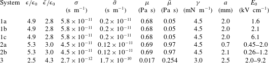
Material properties: systems 1, 2 and 3 correspond to the experiments of Tsukada et al. (Reference Tsukada, Katayama, Ito and Hozawa1993), Salipante & Vlahovska (Reference Salipante and Vlahovska2010) and Lanauze et al. (Reference Lanauze, Walker and Khair2015), respectively.
 $\unicode[STIX]{x1D716}_{0}=8.8542\times 10^{-12}\,\text{F}~\text{m}^{-1}$
denotes the permittivity of vacuum.

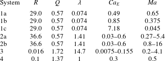
We now compare our theoretical results with existing experimental data, previous small-deformation theories, as well as fully nonlinear numerical simulations using an axisymmetric boundary element method described in appendix C. The material properties, drop sizes and electric field strengths are chosen as in table 1 to match the experimental values of Lanauze et al. (Reference Lanauze, Walker and Khair2015) (system 1), who measured transient drop dynamics, and of Salipante & Vlahovska (Reference Salipante and Vlahovska2010) (system 2) for steady deformations, and corresponding dimensionless parameter values are provided in table 2. Both of these studies considered oblate drops. We also present a few results on prolate drops using the experimental values of Tsukada et al. (Reference Tsukada, Katayama, Ito and Hozawa1993) (system 3) and Ha & Yang (Reference Ha and Yang2000) (system 4). The latter study, however, did not report all the material properties required to construct all five dimensionless parameters in our model; we choose to set the values of the electric capillary number and Mason number to
 $Ca_{E}=0.3$
and
 $Ma=0.5$
in this case.
Dimensionless parameters corresponding to the material properties of table 1: systems 1, 2, 3 and 4 correspond to the experiments of Tsukada et al. (Reference Tsukada, Katayama, Ito and Hozawa1993), Ha & Yang (Reference Ha and Yang2000), Salipante & Vlahovska (Reference Salipante and Vlahovska2010) and Lanauze et al. (Reference Lanauze, Walker and Khair2015), respectively.

Deformation parameter
 ${\mathcal{D}}$
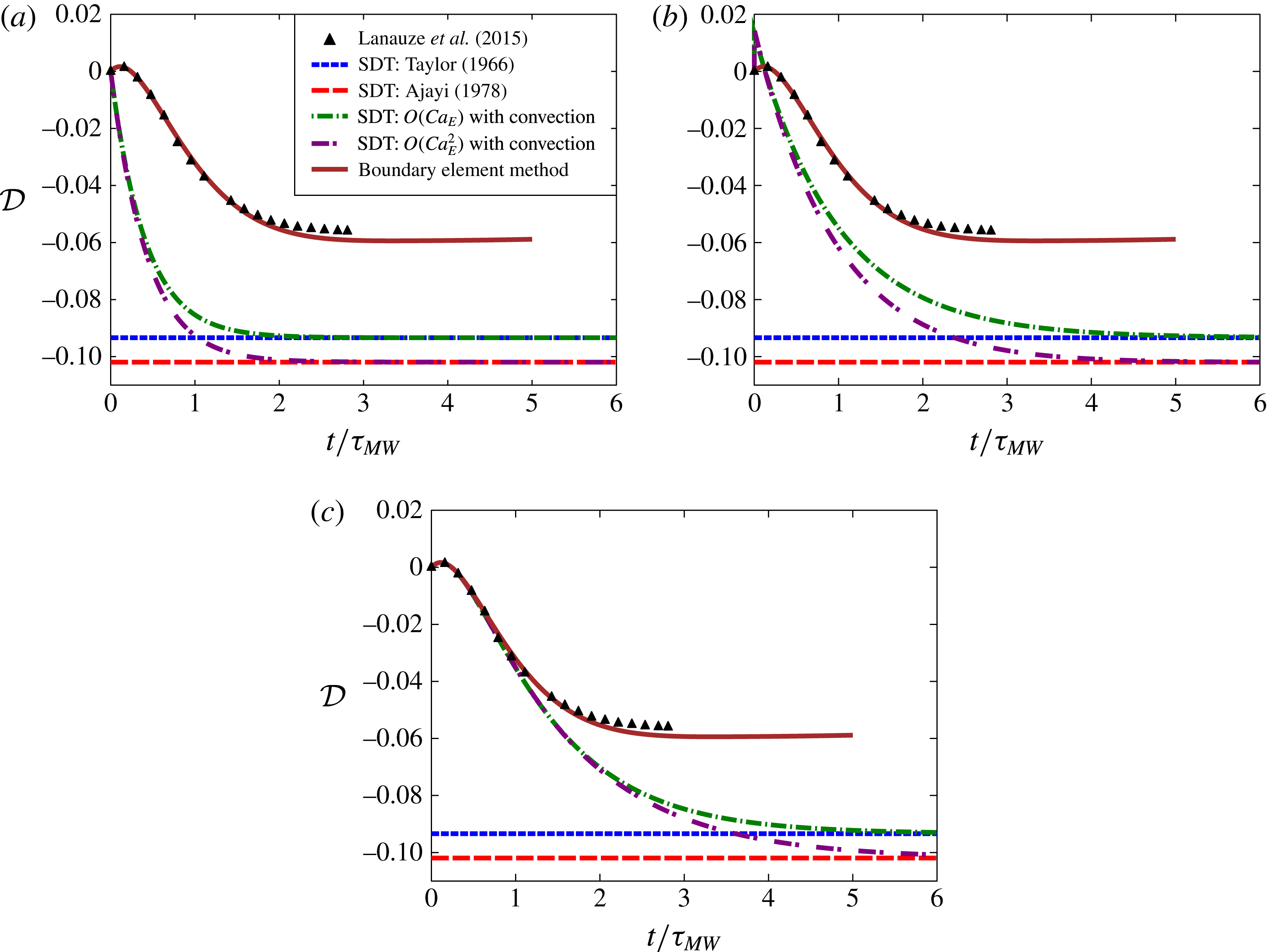
as a function of time for the parameters of system 1b in the absence of charge convection: (
 $a$
) effect of transient shape relaxation only (no transient charge relaxation), (
 $b$
) effect of transient charge relaxation only (no transient shape relaxation), and (
 $c$
) effect of both transient shape and charge relaxation. Symbols show experimental data of Lanauze et al. (Reference Lanauze, Walker and Khair2015). Boundary element simulation results using the full nonlinear model and the algorithm of appendix C are also shown.

5.1 Effect of transient charge relaxation and shape deformation
In this section, we first neglect nonlinear charge convection and focus on the effects of transient charge relaxation and transient shape deformation alone. Here we adopt the experimental values of system 1b. The drop deformation is plotted as a function of time in figure 2 for three distinct cases. In figure 2(
 $a$
), both nonlinear charge convection and transient charge relaxation are neglected. In this case, the only time dependence enters through the temporal derivatives of the shape functions. We find that the drop shape becomes oblate (
 ${\mathcal{D}}<0$
), and our theoretical results asymptote at long times towards the steady-state predictions of Taylor (Reference Taylor1966) and Ajayi (Reference Ajayi1978) at first and second order, respectively. Both steady states, however, overpredict the drop deformation, and it is found, rather curiously, that the theory performs more poorly at second order than at first order; this was already noted by Ajayi (Reference Ajayi1978) and is a consequence of neglecting charge convection, as further discussed below. The transient is also poorly captured: the model predicts a monotonic increase of the drop deformation towards the oblate steady state and fails to capture the initial dynamics seen in experiments, where the drop first adopts a prolate shape before becoming oblate. Figure 2(
 $b$
) shows the opposite situation, in which transient shape deformation is neglected but transient charge relaxation is included. In this case, the shape instantaneously adjusts to the charge distribution, which explains the immediate deformation to a prolate shape at
 $t=0$
as a result of the instantaneous polarization of the drop according to (4.5). The deformation subsequently relaxes monotonically towards its steady oblate value. However, accounting for both transient phenomena in figure 2(
 $c$
) captures the transient dynamics correctly while still evolving towards the steady deformation values of Taylor (Reference Taylor1966) and Ajayi (Reference Ajayi1978) in the absence of charge convection. These results underscore the importance of including all transient effects if one wants to capture the correct shape dynamics.
5.2 Effect of nonlinear charge convection
We now turn to the full theoretical model, which includes transient charge and shape relaxation as well as nonlinear charge convection. As we show here, the main effect of charge convection is to reduce the strength of the interfacial velocity, thereby causing oblate drops to deform less but prolate drops to deform more, in agreement with computational studies (Feng Reference Feng1999; Lanauze et al.
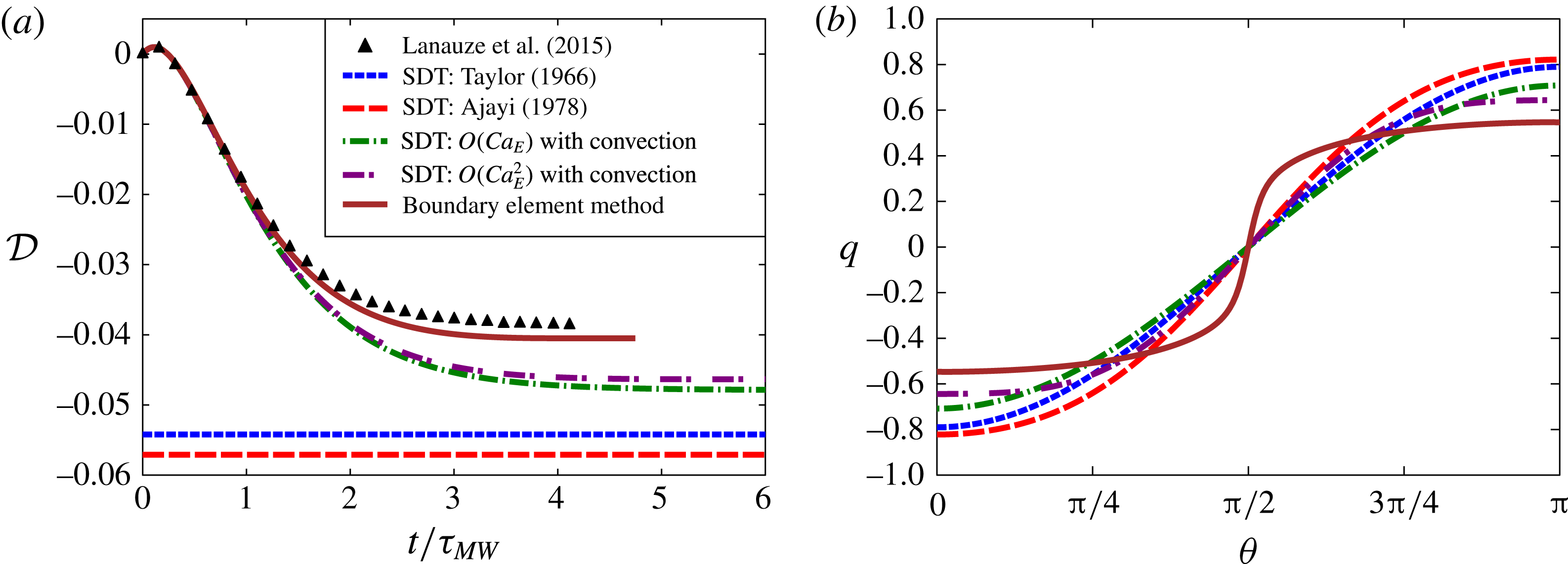
Reference Lanauze, Walker and Khair2015). We first consider the dynamics in a relatively weak electric field using the parameters of system 1a in figure 3. First, we note in figure 3(
 $a$
) that the boundary element simulations perform best and capture both the transient and the steady state with very good accuracy. Our small-deformation theory with charge convection also captures the transient very well, but still slightly overpredicts the steady deformation parameter, albeit not as much as the models of Taylor (Reference Taylor1966) and Ajayi (Reference Ajayi1978). Interestingly, we find that while the second-order theory of Ajayi is worse than the first-order theory of Taylor in the absence of charge convection, such is not the case in our model, where including second-order terms is seen to improve the solution. The poor performance of Ajayi’s model is a direct consequence of the neglect of charge convection, which results in a stronger dipole moment and in turn leads to larger deformations. Charge convection by the flow, on the other hand, causes the transport of positive and negative charges from the poles towards the equator, thus effectively reducing the induced dipole. This point is evident in figure 3(
 $b$
), showing the steady charge distribution on the drop surface, where we see that the second-order theory with charge convection best approximates the charge profile from boundary element simulations. This numerical charge profile, however, exhibits a sharper transition from negative to positive values at the equator.
(
 $a$
) Deformation parameter
 ${\mathcal{D}}$
as a function of time for the parameters of system 1a. (
 $b$
) Steady interfacial charge profile. The plots show experimental results of Lanauze et al. (Reference Lanauze, Walker and Khair2015), fully nonlinear boundary element simulations, first- and second-order small-deformation theory (with nonlinear charge convection), and the steady results of Taylor (Reference Taylor1966) and Ajayi (Reference Ajayi1978) that neglected charge convection.

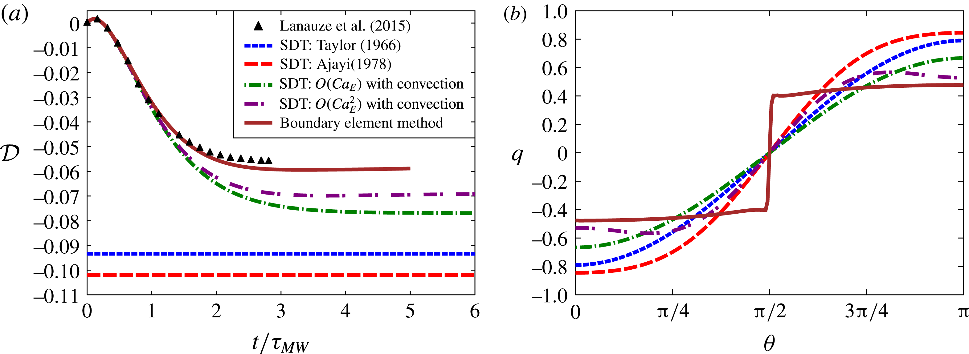
(
 $a$
) Deformation parameter
 ${\mathcal{D}}$
as a function of time for the parameters of system 1b. (
 $b$
) Steady interfacial charge profile. For these parameter values, the charge distribution predicted by the boundary element simulation develops a discontinuity at the equator. See supplementary online materials at https://doi.org/10.1017/jfm.2016.704 for a movie showing the dynamics and flow field in this case.

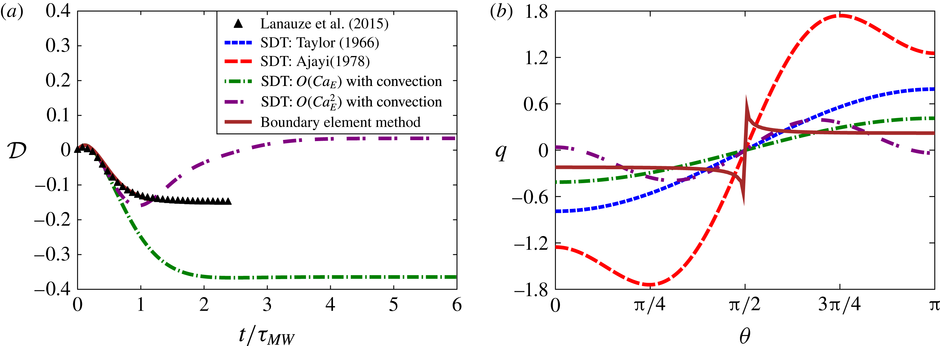
(
 $a$
) Deformation parameter
 ${\mathcal{D}}$
as a function of time for the parameters of system 1c. (
 $b$
) Steady interfacial charge profile. The steady deformation values predicted by the models of Taylor (Reference Taylor1966) and Ajayi (Reference Ajayi1978) in this case are
 $-0.75$
and
 $-1.40$
, respectively, and out of the frame of panel (
 $a$
). For these parameter values, the charge discontinuity at the equator is so severe that the boundary element simulations blow up before reaching steady state; in this case, the charge profile shown in (
 $b$
) corresponds to a time shortly before the instability develops.

The effect of increasing field strength is shown in figure 4, corresponding to system 1b. Unsurprisingly, stronger fields cause larger drop deformations, which are not as easily captured by the theory. While the boundary element simulation matches the experimental data quite well, our nonlinear small-deformation theory captures the transient well but shows a significant departure at steady state. Nevertheless, the second-order theory still outperforms all previous theoretical models. The difficulty in capturing the steady state accurately can be understood by considering the charge profile in figure 4(
 $b$
), where a sharp gradient is observed across the equator in the numerical data from boundary element simulations. This sharp gradient cannot be captured using only two Legendre functions as in the expansion of (3.16), which explains the discrepancy. The problem becomes yet more severe in stronger fields, as shown in figure 5 in the case of system 1c. There, an actual discontinuity appears in the charge profile, leading to the very poor performance of small-deformation theories and to numerical instabilities in the boundary element simulation, which blows up before reaching steady state. The formation of a charge shock in strong fields was first observed in the simulations of Lanauze et al. (Reference Lanauze, Walker and Khair2015), who also were not able to resolve it numerically using their boundary element algorithm based on spline interpolation. The boundary element method used here and described in appendix C solves the charge conservation equation using finite volumes, and yet is still unable to capture the discontinuity, suggesting that higher-order non-oscillating numerical schemes should be employed towards this purpose (LeVeque Reference Leveque2002).
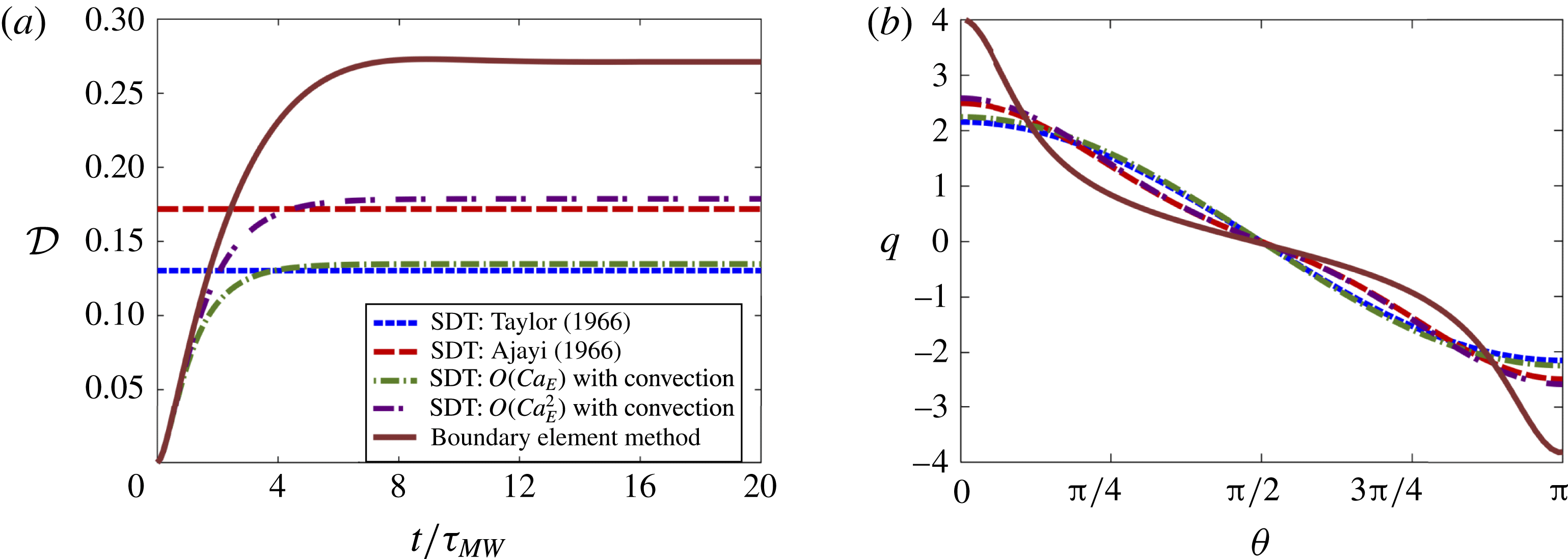
(
 $a$
) Deformation parameter
 ${\mathcal{D}}$
as a function of time for the parameters of system 4, which correspond to a steady prolate shape. (
 $b$
) Steady interfacial charge profile.

The case of prolate deformations is illustrated in figure 6 using the parameters of system 4. In this case, the drop deformation increases monotonically with time. The steady deformation parameter obtained by simulations with
 $Ma=0.5$
is
 ${\mathcal{D}}=0.27$
, which slightly exceeds the value of
 ${\mathcal{D}}=0.22$
found by Lac & Homsy (Reference Lac and Homsy2007), who neglected charge convection (
 $Ma\rightarrow \infty$
); the experiments of Ha & Yang (Reference Ha and Yang2000), for which the value of
 $Ma$
is unknown, reported a deformation of
 ${\mathcal{D}}=0.25$
. Our small-deformation theory only provides a modest improvement at steady state over the predictions of Taylor (Reference Taylor1966) and Ajayi (Reference Ajayi1978), again confirming that nonlinear charge convection has a weaker effect for prolate drops. This again can be rationalized by considering the interfacial charge profile in figure 6(
 $b$
): convection by the flow is seen to cause charge accumulation at the drop poles, and thus does not cause any discontinuity as in the oblate case. Instead, the charge profile remains relatively smooth and therefore can be reasonably well approximated using Legendre polynomials.
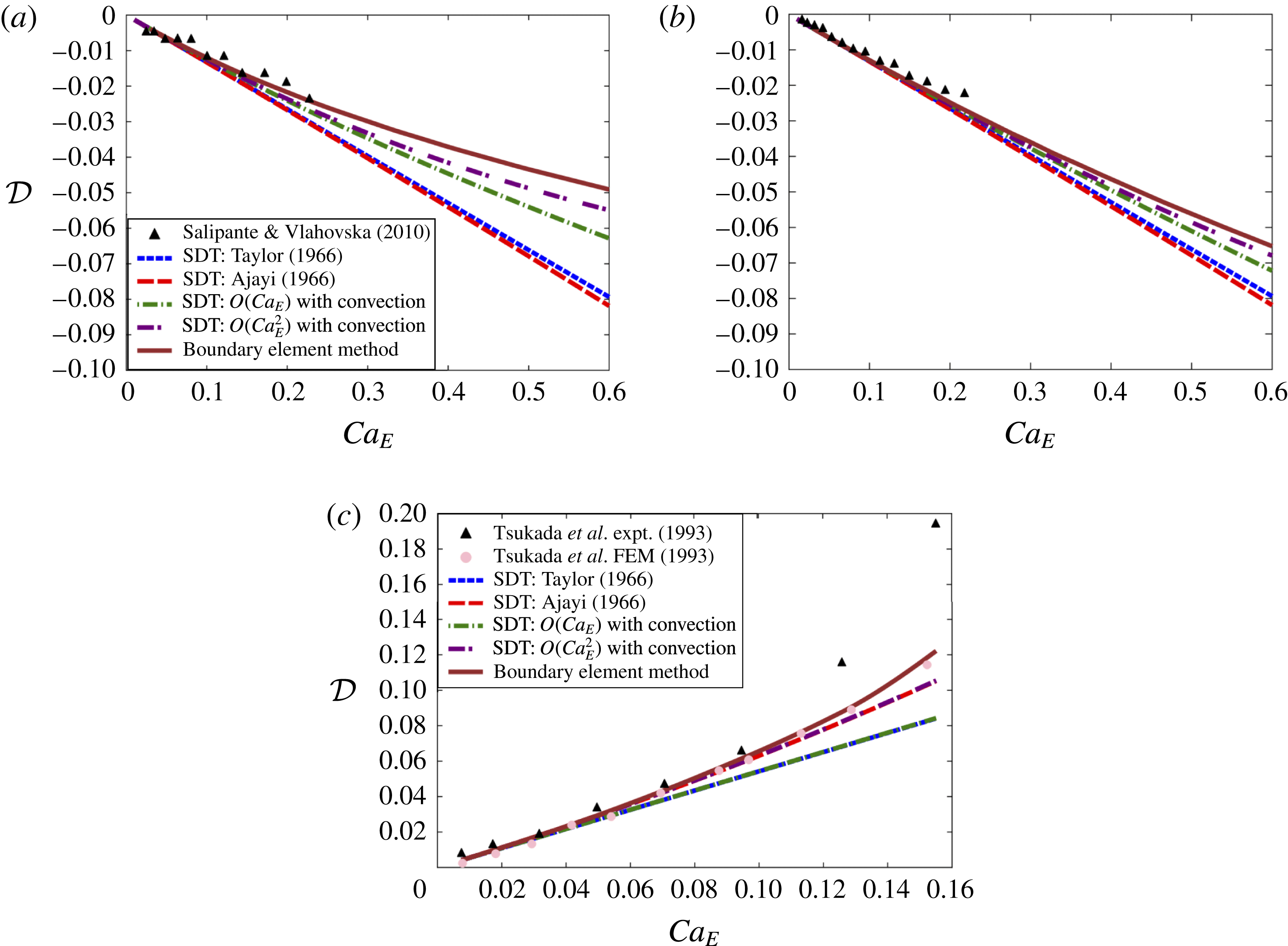
Steady drop deformation
 ${\mathcal{D}}$
as a function of electric capillary number
 $Ca_{E}$
for the parameters of: (
 $a$
) system 2a, (
 $b$
) system 2b, and (
 $c$
) system 3. The various models are compared to the experimental measurements of Tsukada et al. (Reference Tsukada, Katayama, Ito and Hozawa1993) and Salipante & Vlahovska (Reference Salipante and Vlahovska2010).

As a final test, we compare our theoretical and numerical predictions for the steady drop shapes with the experimental results of Salipante & Vlahovska (Reference Salipante and Vlahovska2010) for systems 2a and 2b, with oblate drops, and Tsukada et al. (Reference Tsukada, Katayama, Ito and Hozawa1993) for system 3, with prolate drops, in figure 7. The experimental system 2 used two different drop sizes but identical material properties. At a given value of the electric capillary number
 $Ca_{E}$
, increasing drop size is equivalent to decreasing the electric field or increasing the Mason number
 $Ma$
, which reduces the effect of charge convection. Charge convection is therefore more significant in figure 7(
 $a$
) for the smaller drop size, and indeed departures of our numerical and theoretical results from the small-deformation theories of Taylor (Reference Taylor1966) and Ajayi (Reference Ajayi1978) are more significant in this case. In both cases, our theoretical model performs quite well at predicting the steady drop shape, but still slightly overpredicts the experimental values, especially as
 $Ca_{E}$
increases; nonetheless the agreement is noticeably better than in previous models. The effect of charge convection is extremely weak in the case of prolate drops in system 3, as shown in figure 7(
 $c$
). As a consequence, our first- and second-order theories are indistinguishable from Taylor’s and Ajayi’s results, and the deformations predicted by our axisymmetric boundary element method only slightly exceed the finite-element simulation values of Tsukada et al. (Reference Tsukada, Katayama, Ito and Hozawa1993), who neglected charge convection.
6 Concluding remarks
In summary, we have developed a small-deformation theory for the complete Melcher–Taylor leaky dielectric model including the nonlinear charge convection term. The theory is most relevant for small-sized drops or drops with high surface tension but non-negligible charge convection. A domain perturbation method based on spherical harmonics valid for small deviations from sphericity was employed to represent the drop shape up to second order in electric capillary number
 $O(Ca_{E}^{2})$
. The zeroth- and first-order electric and flow fields were solved for using multipole expansions. On making the appropriate assumptions, we were able to recover the previous theoretical models (Taylor Reference Taylor1966; Ajayi Reference Ajayi1978; Esmaeeli & Sharifi Reference Esmaeeli and Sharifi2011; Lanauze et al.
Reference Lanauze, Walker and Khair2013). The discrepancy of Ajayi’s second-order theory predicting drop deformation more inaccurately than Taylor’s first-order theory in the case of oblate drops was resolved by including charge convection in the theoretical model. Retention of transient charge relaxation and shape deformation was also shown to be critical in order to accurately capture the transient non-monotonic drop deformation, as we validated by comparison with both numerical simulations and existing experimental data.
While our second-order theory showed good agreement with simulations and experiments, departures become significant with increasing electric field strength as deformations become larger. While possible in principle, extending the theory to include higher-order corrections in
 $Ca_{E}$
is exceedingly difficult due to the nonlinearities in the governing equations. The problem of capturing large deformations in a theoretical model would likely be better addressed using spheroidal coordinates, as in the previous work of Zhang, Zahn & Lin (Reference Zhang, Zahn and Lin2013), though this method has yet to be adapted to include charge convection. One should also note that the present study is limited to axisymmetric drop deformations. In strong electric fields, experiments have demonstrated the existence of a symmetry-breaking bifurcation leading to Quincke electrorotation (Salipante & Vlahovska Reference Salipante and Vlahovska2010, Reference Salipante and Vlahovska2013; He, Salipante & Vlahovska Reference He, Salipante and Vlahovska2013), which is characterized by non-axisymmetric shapes and a primarily rotational flow. Such effects cannot be captured by the theory and simulations presented herein. From a theoretical standpoint, a fully three-dimensional model would preclude the simple use of a Stokes streamfunction as done in § 3.3 for the solution of the flow problem, which could instead by obtained using Lamb’s general solution of the Stokes equations (Kim & Karrila Reference Kim and Karrila2013). Such a model would also be useful for the description of pair interactions between widely separated drops using the method of reflections, in a similar manner as in the previous work of Anderson (Reference Anderson1985) for thermocapillary motion of drops, or as in our previous theory for electrohydrodynamic interactions between rigid spheres (Das & Saintillan Reference Das and Saintillan2013); the understanding of such interactions could then pave the way for dilute suspension theories for electrohydrodynamics of multiple drops. Lastly, three-dimensional boundary element simulations would be of great use to describe large deformations and electrorotation in strong fields, and are the subject of our current work.
Acknowledgements
The authors thank P. Vlahovska and P. Salipante for comments and suggestions, A. Khair and J. Lanauze for useful discussions and for sharing their experimental data, and L. Rossini for help with generating movies of drop dynamics. We acknowledge the Donors of the American Chemical Society Petroleum Research Fund for partial support of this research through grant 53240-ND9.
Supplementary movies
Supplementary movies are available at https://doi.org/10.1017/jfm.2016.704.
Appendix A. Expansion coefficients for the electric problem
The normal and tangential components of the electric field are expressed in terms of the dipole and octupole moments as:
 $$\begin{eqnarray}\displaystyle E_{01}^{n}=1+2P_{01},\quad \bar{E}_{01}^{n}=1-P_{01}, & & \displaystyle\end{eqnarray}$$
 $$\begin{eqnarray}\displaystyle E_{11}^{n}=2P_{11}-{\textstyle \frac{6}{5}}f_{12}(1+P_{01}),\quad \bar{E}_{11}^{n}=-P_{11}-{\textstyle \frac{6}{5}}f_{12}(1-2P_{01}), & & \displaystyle\end{eqnarray}$$
 $$\begin{eqnarray}\displaystyle E_{13}^{n}=4P_{13}+{\textstyle \frac{6}{5}}f_{12}(1-4P_{01}),\quad \bar{E}_{13}^{n}=-3P_{13}+{\textstyle \frac{6}{5}}f_{12}\left(1+{\textstyle \frac{7}{2}}P_{01}\right), & & \displaystyle\end{eqnarray}$$
 $$\begin{eqnarray}\displaystyle E_{00}^{t} & = & \displaystyle -(1-P_{01}),\end{eqnarray}$$
 $$\begin{eqnarray}\displaystyle E_{10}^{t} & = & \displaystyle P_{13}+P_{11}-f_{12}(1+2P_{01}),\end{eqnarray}$$
 $$\begin{eqnarray}\displaystyle E_{12}^{t} & = & \displaystyle 5P_{13}-f_{12}(2+7P_{01}).\end{eqnarray}$$
 $$\begin{eqnarray}\displaystyle q_{01} & = & \displaystyle E_{01}^{n}-Q\bar{E}_{01}^{n}=1+2P_{01}-Q(1-P_{01}),\end{eqnarray}$$
 $$\begin{eqnarray}\displaystyle q_{11} & = & \displaystyle E_{11}^{n}-Q\bar{E}_{11}^{n}=2P_{11}-{\textstyle \frac{6}{5}}f_{12}(1+P_{01})-Q[-P_{11}-{\textstyle \frac{6}{5}}f_{12}(1-2P_{01})],\end{eqnarray}$$
 $$\begin{eqnarray}\displaystyle q_{13} & = & \displaystyle E_{13}^{n}-Q\bar{E}_{13}^{n}=4P_{13}+{\textstyle \frac{6}{5}}f_{12}(1-4P_{01})-Q[-3P_{13}+{\textstyle \frac{6}{5}}f_{12}\left(1+{\textstyle \frac{7}{2}}P_{01}\right)],\end{eqnarray}$$
 $$\begin{eqnarray}\displaystyle \unicode[STIX]{x27E6}\,j\unicode[STIX]{x27E7}_{01}^{n} & = & \displaystyle RE_{01}^{n}-\bar{E}_{01}^{n}=R(1+2P_{01})-1+P_{01},\end{eqnarray}$$
 $$\begin{eqnarray}\displaystyle \unicode[STIX]{x27E6}\,j\unicode[STIX]{x27E7}_{11}^{n} & = & \displaystyle RE_{11}^{n}-\bar{E}_{11}^{n}=R[2P_{11}-{\textstyle \frac{6}{5}}f_{12}(1+P_{01})]+P_{11}+{\textstyle \frac{6}{5}}f_{12}(1-2P_{01}),\end{eqnarray}$$
 $$\begin{eqnarray}\displaystyle \unicode[STIX]{x27E6}\,j\unicode[STIX]{x27E7}_{13}^{n} & = & \displaystyle RE_{13}^{n}-\bar{E}_{13}^{n}=R[4P_{13}+{\textstyle \frac{6}{5}}f_{12}(1-4P_{01})]+3P_{13}-{\textstyle \frac{6}{5}}f_{12}\left(1+{\textstyle \frac{7}{2}}P_{01}\right).\end{eqnarray}$$
 $$\begin{eqnarray}\displaystyle [qE^{t}]_{01} & = & \displaystyle q_{01}E_{01}^{t},\end{eqnarray}$$
 $$\begin{eqnarray}\displaystyle [qE^{t}]_{11} & = & \displaystyle q_{01}E_{11}^{t}+{\textstyle \frac{2}{5}}q_{01}E_{13}^{t}+q_{11}E_{01}^{t},\end{eqnarray}$$
 $$\begin{eqnarray}\displaystyle [qE^{t}]_{13} & = & \displaystyle {\textstyle \frac{3}{5}}q_{01}E_{13}^{t}+q_{13}E_{01}^{t},\end{eqnarray}$$
 $$\begin{eqnarray}\displaystyle \unicode[STIX]{x27E6}\,p^{E}\unicode[STIX]{x27E7}_{00} & = & \displaystyle {\textstyle \frac{1}{6}}(E_{01}^{n2}-Q\bar{E}_{01}^{n2})+{\textstyle \frac{1}{3}}(Q-1)E_{00}^{t2},\end{eqnarray}$$
 $$\begin{eqnarray}\displaystyle \unicode[STIX]{x27E6}\,p^{E}\unicode[STIX]{x27E7}_{02} & = & \displaystyle {\textstyle \frac{1}{3}}(E_{01}^{n2}-Q\bar{E}_{01}^{n2})-{\textstyle \frac{1}{3}}(Q-1)E_{00}^{t2},\end{eqnarray}$$
 $$\begin{eqnarray}\displaystyle \unicode[STIX]{x27E6}\,p^{E}\unicode[STIX]{x27E7}_{10} & = & \displaystyle {\textstyle \frac{1}{3}}(E_{01}^{n}E_{11}^{n}-Q\bar{E}_{01}^{n}\bar{E}_{11}^{n})+{\textstyle \frac{2}{3}}E_{00}^{t}(E_{10}^{t}-{\textstyle \frac{1}{5}}E_{12}^{t}),\end{eqnarray}$$
 $$\begin{eqnarray}\displaystyle \unicode[STIX]{x27E6}\,p^{E}\unicode[STIX]{x27E7}_{12} & = & \displaystyle {\textstyle \frac{2}{3}}(E_{01}^{n}E_{11}^{n}-Q\bar{E}_{01}^{n}\bar{E}_{11}^{n})+{\textstyle \frac{3}{7}}(E_{01}^{n}E_{13}^{n}-Q\bar{E}_{01}^{n}\bar{E}_{13}^{n})+{\textstyle \frac{2}{3}}E_{00}^{t}({\textstyle \frac{5}{7}}E_{12}^{t}-E_{10}^{t})\end{eqnarray}$$
 $$\begin{eqnarray}\displaystyle \unicode[STIX]{x27E6}\,p^{E}\unicode[STIX]{x27E7}_{14} & = & \displaystyle {\textstyle \frac{4}{7}}(E_{01}^{n}E_{13}^{n}-Q\bar{E}_{01}^{n}\bar{E}_{13}^{n})-{\textstyle \frac{12}{35}}E_{00}^{t}E_{12}^{t},\end{eqnarray}$$
Appendix B. Expansion coefficients for the flow problem
The zeroth-order coefficients of the normal and tangential components of the interfacial velocity used in (3.29) are found to be
 $$\begin{eqnarray}\displaystyle v_{02}^{n}=A_{03}+B_{03},\quad \bar{v}_{02}^{n}=\bar{A}_{03}+\bar{B}_{03}, & & \displaystyle\end{eqnarray}$$
 $$\begin{eqnarray}\displaystyle v_{01}^{t}=A_{03},\quad \bar{v}_{01}^{t}=-{\textstyle \frac{3}{2}}\bar{A}_{03}-{\textstyle \frac{5}{2}}\bar{B}_{03}. & & \displaystyle\end{eqnarray}$$
 $$\begin{eqnarray}\displaystyle v_{10}^{n} & = & \displaystyle -{\textstyle \frac{2}{5}}f_{12}(A_{03}+B_{03}),\end{eqnarray}$$
 $$\begin{eqnarray}\displaystyle v_{12}^{n} & = & \displaystyle A_{13}+B_{13}-{\textstyle \frac{2}{7}}f_{12}(3A_{03}+2B_{03}),\end{eqnarray}$$
 $$\begin{eqnarray}\displaystyle v_{14}^{n} & = & \displaystyle A_{15}+B_{15}-{\textstyle \frac{12}{35}}f_{12}(8A_{03}+3B_{03}),\end{eqnarray}$$
 $$\begin{eqnarray}\displaystyle \bar{v}_{10}^{n} & = & \displaystyle -{\textstyle \frac{2}{5}}f_{12}(\bar{A}_{03}+\bar{B}_{03}),\end{eqnarray}$$
 $$\begin{eqnarray}\displaystyle \bar{v}_{12}^{n} & = & \displaystyle \bar{A}_{13}+\bar{B}_{13}-{\textstyle \frac{1}{7}}f_{12}(\bar{A}_{03}-\bar{B}_{03}),\end{eqnarray}$$
 $$\begin{eqnarray}\displaystyle \bar{v}_{14}^{n} & = & \displaystyle \bar{A}_{15}+\bar{B}_{15}+{\textstyle \frac{6}{35}}f_{12}(9\bar{A}_{03}+19\bar{B}_{03}),\end{eqnarray}$$
 $$\begin{eqnarray}\displaystyle v_{11}^{t} & = & \displaystyle A_{13}+{\textstyle \frac{3}{5}}A_{15}+{\textstyle \frac{3}{10}}B_{15}-{\textstyle \frac{2}{5}}f_{12}(7A_{03}+3B_{03}),\end{eqnarray}$$
 $$\begin{eqnarray}\displaystyle v_{13}^{t} & = & \displaystyle {\textstyle \frac{7}{5}}A_{15}+{\textstyle \frac{7}{10}}B_{15}-{\textstyle \frac{3}{5}}f_{12}(7A_{03}+3B_{03}),\end{eqnarray}$$
 $$\begin{eqnarray}\displaystyle \bar{v}_{11}^{t} & = & \displaystyle -{\textstyle \frac{3}{2}}\bar{A}_{13}-{\textstyle \frac{5}{2}}\bar{B}_{13}-{\textstyle \frac{3}{4}}\bar{A}_{15}-{\textstyle \frac{21}{20}}\bar{B}_{15}-{\textstyle \frac{3}{5}}f_{12}(3\bar{A}_{03}+7\bar{B}_{03}),\end{eqnarray}$$
 $$\begin{eqnarray}\displaystyle \bar{v}_{13}^{t} & = & \displaystyle -{\textstyle \frac{7}{4}}\bar{A}_{15}-{\textstyle \frac{49}{20}}\bar{B}_{15}-{\textstyle \frac{9}{10}}f_{12}(3\bar{A}_{03}+7\bar{B}_{03}).\end{eqnarray}$$
 $$\begin{eqnarray}\displaystyle A_{03}=-B_{03}+\unicode[STIX]{x1D6FF}{\dot{f}}_{12},\quad \bar{A}_{03}=-B_{03}+{\textstyle \frac{7}{2}}\unicode[STIX]{x1D6FF}{\dot{f}}_{12},\quad \bar{B}_{03}=B_{03}-{\textstyle \frac{5}{2}}\unicode[STIX]{x1D6FF}{\dot{f}}_{12}. & & \displaystyle\end{eqnarray}$$
Using these relations together with the condition that
 $f_{20}=-f_{12}^{2}/5$
obtained in § 3.1 from volume conservation, it is easy to show that (3.30b
) is trivially satisfied. The remaining first-order boundary conditions then yield six additional equations that can be combined to show that
 $$\begin{eqnarray}\displaystyle A_{13} & = & \displaystyle -B_{13}-{\textstyle \frac{2}{7}}f_{12}B_{03}+\unicode[STIX]{x1D6FF}{\dot{f}}_{22}+{\textstyle \frac{6}{7}}\unicode[STIX]{x1D6FF}f_{12}{\dot{f}}_{12},\end{eqnarray}$$
 $$\begin{eqnarray}\displaystyle \bar{A}_{13} & = & \displaystyle -B_{13}+{\textstyle \frac{3}{7}}f_{12}B_{03}+{\textstyle \frac{7}{2}}\unicode[STIX]{x1D6FF}{\dot{f}}_{22}+{\textstyle \frac{1}{2}}\unicode[STIX]{x1D6FF}f_{12}{\dot{f}}_{12},\end{eqnarray}$$
 $$\begin{eqnarray}\displaystyle \bar{B}_{13} & = & \displaystyle B_{13}-{\textstyle \frac{5}{7}}f_{12}B_{03}-{\textstyle \frac{5}{2}}\unicode[STIX]{x1D6FF}{\dot{f}}_{22}+{\textstyle \frac{5}{14}}\unicode[STIX]{x1D6FF}f_{12}{\dot{f}}_{12},\end{eqnarray}$$
 $$\begin{eqnarray}\displaystyle A_{15} & = & \displaystyle -B_{15}-{\textstyle \frac{12}{7}}f_{12}B_{03}+\unicode[STIX]{x1D6FF}{\dot{f}}_{24}+{\textstyle \frac{96}{35}}\unicode[STIX]{x1D6FF}f_{12}{\dot{f}}_{12},\end{eqnarray}$$
 $$\begin{eqnarray}\displaystyle \bar{A}_{15} & = & \displaystyle -B_{15}-{\textstyle \frac{6}{7}}f_{12}B_{03}+{\textstyle \frac{11}{2}}\unicode[STIX]{x1D6FF}{\dot{f}}_{24}+{\textstyle \frac{3}{35}}\unicode[STIX]{x1D6FF}f_{12}{\dot{f}}_{12},\end{eqnarray}$$
 $$\begin{eqnarray}\displaystyle \bar{B}_{15} & = & \displaystyle B_{15}-{\textstyle \frac{6}{7}}f_{12}B_{03}-{\textstyle \frac{9}{2}}\unicode[STIX]{x1D6FF}{\dot{f}}_{24}+{\textstyle \frac{93}{35}}\unicode[STIX]{x1D6FF}f_{12}{\dot{f}}_{12}.\end{eqnarray}$$
 $B_{03}$
,
 $B_{13}$
and
 $B_{15}$
. The hydrodynamic stress is obtained by using (3.35). At zeroth order, we find:
 $$\begin{eqnarray}\displaystyle \unicode[STIX]{x27E6}T^{H}\unicode[STIX]{x27E7}_{00}^{nn} & = & \displaystyle \unicode[STIX]{x27E6}\,p^{H}\unicode[STIX]{x27E7}_{00},\end{eqnarray}$$
 $$\begin{eqnarray}\displaystyle \unicode[STIX]{x27E6}T^{H}\unicode[STIX]{x27E7}_{02}^{nn} & = & \displaystyle (2+3\unicode[STIX]{x1D706})B_{03}-{\textstyle \frac{1}{2}}(16+19\unicode[STIX]{x1D706})\unicode[STIX]{x1D6FF}{\dot{f}}_{12},\end{eqnarray}$$
 $$\begin{eqnarray}\displaystyle \unicode[STIX]{x27E6}T^{H}\unicode[STIX]{x27E7}_{01}^{nt} & = & \displaystyle 5(1+\unicode[STIX]{x1D706})B_{03}-{\textstyle \frac{1}{2}}(16+19\unicode[STIX]{x1D706})\unicode[STIX]{x1D6FF}{\dot{f}}_{12}.\end{eqnarray}$$
 $$\begin{eqnarray}\displaystyle \unicode[STIX]{x27E6}T^{H}\unicode[STIX]{x27E7}_{10}^{nn} & = & \displaystyle \unicode[STIX]{x27E6}\,p^{H}\unicode[STIX]{x27E7}_{10}+{\textstyle \frac{2}{5}}(-1+11\unicode[STIX]{x1D706})B_{03}f_{12}+{\textstyle \frac{1}{5}}(8-43\unicode[STIX]{x1D706})\unicode[STIX]{x1D6FF}{\dot{f}}_{12}f_{12},\end{eqnarray}$$
 $$\begin{eqnarray}\displaystyle \unicode[STIX]{x27E6}T^{H}\unicode[STIX]{x27E7}_{12}^{nn} & = & \displaystyle (2+3\unicode[STIX]{x1D706})B_{13}+{\textstyle \frac{1}{7}}(-8+13\unicode[STIX]{x1D706})B_{03}f_{12}-{\textstyle \frac{1}{2}}(16+19\unicode[STIX]{x1D706})\unicode[STIX]{x1D6FF}{\dot{f}}_{22}\nonumber\\ \displaystyle & & \displaystyle -{\textstyle \frac{105}{14}}\unicode[STIX]{x1D706}\,\unicode[STIX]{x1D6FF}f_{12}{\dot{f}}_{12},\end{eqnarray}$$
 $$\begin{eqnarray}\displaystyle \unicode[STIX]{x27E6}T^{H}\unicode[STIX]{x27E7}_{14}^{nn} & = & \displaystyle {\textstyle \frac{3}{10}}(4+5\unicode[STIX]{x1D706})B_{15}+{\textstyle \frac{3}{35}}(28+37\unicode[STIX]{x1D706})B_{03}f_{12}-{\textstyle \frac{3}{4}}(16+17\unicode[STIX]{x1D706})\unicode[STIX]{x1D6FF}{\dot{f}}_{24}\nonumber\\ \displaystyle & & \displaystyle -{\textstyle \frac{3}{70}}(32+47\unicode[STIX]{x1D706})\unicode[STIX]{x1D6FF}f_{12}{\dot{f}}_{12},\end{eqnarray}$$
 $$\begin{eqnarray}\displaystyle \unicode[STIX]{x27E6}T^{H}\unicode[STIX]{x27E7}_{11}^{nt} & = & \displaystyle 5(1+\unicode[STIX]{x1D706})B_{13}+{\textstyle \frac{27}{10}}(1+\unicode[STIX]{x1D706})B_{15}-{\textstyle \frac{4}{35}}(33+18\unicode[STIX]{x1D706})B_{03}f_{12}\nonumber\\ \displaystyle & & \displaystyle -{\textstyle \frac{1}{2}}(16+19\unicode[STIX]{x1D706})\unicode[STIX]{x1D6FF}{\dot{f}}_{22}-{\textstyle \frac{9}{20}}(16+17\unicode[STIX]{x1D706})\unicode[STIX]{x1D6FF}{\dot{f}}_{24}+{\textstyle \frac{2}{175}}(227-466\unicode[STIX]{x1D706})\unicode[STIX]{x1D6FF}f_{12}{\dot{f}}_{12},\end{eqnarray}$$
 $$\begin{eqnarray}\displaystyle \unicode[STIX]{x27E6}T^{H}\unicode[STIX]{x27E7}_{13}^{nt} & = & \displaystyle {\textstyle \frac{63}{10}}(1+\unicode[STIX]{x1D706})B_{15}-{\textstyle \frac{9}{5}}(1+\unicode[STIX]{x1D706})B_{03}f_{12}-{\textstyle \frac{21}{20}}(16+17\unicode[STIX]{x1D706})\unicode[STIX]{x1D6FF}{\dot{f}}_{24}\nonumber\\ \displaystyle & & \displaystyle +\,{\textstyle \frac{9}{50}}(4-7\unicode[STIX]{x1D706})\unicode[STIX]{x1D6FF}f_{12}{\dot{f}}_{12}.\end{eqnarray}$$
 $\unicode[STIX]{x27E6}\,p^{H}\unicode[STIX]{x27E7}_{00}$
and
 $\unicode[STIX]{x27E6}\,p^{H}\unicode[STIX]{x27E7}_{10}$
denote uniform hydrostatic pressure jumps that do not affect drop shape.
Appendix C. Axisymmetric boundary element method
We outline the numerical method used in § 5 for the solution of the full nonlinear problem in axisymmetric geometry based on boundary integral equations (Jaswon Reference Jaswon1963; Symm Reference Symm1963). The method shares similarities with that of Lanauze et al. (Reference Lanauze, Walker and Khair2015), but makes use of a finite-volume algorithm for the solution of the charge convection equation. We first solve Laplace’s equation for the electric potential using a single-layer potential (Sherwood Reference Sherwood1988; Baygents, Rivette & Stone Reference Baygents, Rivette and Stone1998; Lac & Homsy Reference Lac and Homsy2007; Lanauze et al. Reference Lanauze, Walker and Khair2015), yielding the integral equation
 $$\begin{eqnarray}\displaystyle \unicode[STIX]{x1D711}(\boldsymbol{x}_{0})=-\boldsymbol{x}_{0}\boldsymbol{\cdot }\boldsymbol{E}_{0}+\int _{C}\unicode[STIX]{x27E6}E^{n}(\boldsymbol{x})\unicode[STIX]{x27E7}\,{\mathcal{G}}^{a}(\boldsymbol{x}_{0};\boldsymbol{x})\,\text{d}s(\boldsymbol{x}), & & \displaystyle\end{eqnarray}$$
where
 $C$
is the one-dimensional curve describing the drop shape, which is parametrized by arclength
 $s$
. Equation (C 1) is valid for any location of the evaluation point
 $\boldsymbol{x}_{0}$
on the drop surface
 $C$
or in either of the fluid domains
 $V$
and
 $\bar{V}$
. It involves the axisymmetric Green’s function for Laplace’s equation, which is obtained by integration of the three-dimensional free-space Green’s function over the azimuthal direction:
 $$\begin{eqnarray}{\mathcal{G}}^{a}(\boldsymbol{x}_{0};\boldsymbol{x})=\int _{0}^{2\unicode[STIX]{x03C0}}\frac{\text{d}\unicode[STIX]{x1D719}}{4\unicode[STIX]{x03C0}r},\quad \text{where }r=|\boldsymbol{r}|=|\boldsymbol{x}_{0}-\boldsymbol{x}|.\end{eqnarray}$$
Knowledge of the single-layer potential density
 $\unicode[STIX]{x27E6}E^{n}\unicode[STIX]{x27E7}$
therefore allows determination of the electric potential anywhere in space by simple integration, which prompts us to seek an equation for
 $\unicode[STIX]{x27E6}E^{n}\unicode[STIX]{x27E7}$
in terms of the charge density
 $q$
. To this end, we first take the gradient of (C 1) with respect to
 $\boldsymbol{x}_{0}$
to obtain integral equations for the electric field in both fluid phases:
 $$\begin{eqnarray}\displaystyle \boldsymbol{E}(\boldsymbol{x}_{0}) & = & \displaystyle \boldsymbol{E}_{0}-\int _{C}\unicode[STIX]{x27E6}E^{n}(\boldsymbol{x})\unicode[STIX]{x27E7}\unicode[STIX]{x1D735}_{0}{\mathcal{G}}^{a}\,\text{d}s(\boldsymbol{x})\quad \text{for }\boldsymbol{x}_{0}\in V,\end{eqnarray}$$
 $$\begin{eqnarray}\displaystyle \bar{\boldsymbol{E}}(\boldsymbol{x}_{0}) & = & \displaystyle \boldsymbol{E}_{0}-\int _{C}\unicode[STIX]{x27E6}E^{n}(\boldsymbol{x})\unicode[STIX]{x27E7}\unicode[STIX]{x1D735}_{0}{\mathcal{G}}^{a}\,\text{d}s(\boldsymbol{x})\quad \text{for }\boldsymbol{x}_{0}\in \bar{V}.\end{eqnarray}$$
 $$\begin{eqnarray}\displaystyle \boldsymbol{E}(\boldsymbol{x}_{0}) & = & \displaystyle \boldsymbol{E}_{0}-\int _{C}\unicode[STIX]{x27E6}E^{n}(\boldsymbol{x})\unicode[STIX]{x27E7}\unicode[STIX]{x1D735}_{0}{\mathcal{G}}^{a}\,\text{d}s(\boldsymbol{x})+{\textstyle \frac{1}{2}}\unicode[STIX]{x27E6}E^{n}(\boldsymbol{x}_{0})\unicode[STIX]{x27E7}\boldsymbol{n}(\boldsymbol{x}_{0})\quad \text{for }\boldsymbol{x}_{0}\in C,\end{eqnarray}$$
 $$\begin{eqnarray}\displaystyle \bar{\boldsymbol{E}}(\boldsymbol{x}_{0}) & = & \displaystyle \boldsymbol{E}_{0}-\int _{C}\unicode[STIX]{x27E6}E^{n}(\boldsymbol{x})\unicode[STIX]{x27E7}\unicode[STIX]{x1D735}_{0}{\mathcal{G}}^{a}\,\text{d}s(\boldsymbol{x})-{\textstyle \frac{1}{2}}\unicode[STIX]{x27E6}E^{n}(\boldsymbol{x}_{0})\unicode[STIX]{x27E7}\boldsymbol{n}(\boldsymbol{x}_{0})\quad \text{for }\boldsymbol{x}_{0}\in C.\end{eqnarray}$$
 $\boldsymbol{x}=\boldsymbol{x}_{0}$
, though the singularity disappears after taking the dot product with the normal
 $\boldsymbol{n}(\boldsymbol{x}_{0})$
. An integral equation for the jump can then be obtained by summing both equations and combining them with Gauss’s law (2.4), which is written
 $q=E^{n}-Q\bar{E}^{n}$
in dimensionless form. After manipulations, it reads
 $$\begin{eqnarray}\displaystyle \int _{C}\unicode[STIX]{x27E6}E^{n}(\boldsymbol{x})\unicode[STIX]{x27E7}[\boldsymbol{n}(\boldsymbol{x}_{0})\boldsymbol{\cdot }\unicode[STIX]{x1D735}_{0}{\mathcal{G}}^{a}]\text{d}s(\boldsymbol{x})-\frac{1+Q}{2(1-Q)}\unicode[STIX]{x27E6}E^{n}(\boldsymbol{x}_{0})\unicode[STIX]{x27E7}=E_{0}^{n}(\boldsymbol{x}_{0})-\frac{q(\boldsymbol{x}_{0})}{1-Q}. & & \displaystyle\end{eqnarray}$$
This can be solved for
 $\unicode[STIX]{x27E6}E^{n}\unicode[STIX]{x27E7}$
, from which
 $E^{n}$
and
 $\bar{E}^{n}$
are deduced using Gauss’s law as
 $$\begin{eqnarray}E^{n}=\frac{q-Q\unicode[STIX]{x27E6}E^{n}\unicode[STIX]{x27E7}}{1-Q},\quad \bar{E}^{n}=\frac{q-\unicode[STIX]{x27E6}E^{n}\unicode[STIX]{x27E7}}{1-Q}.\end{eqnarray}$$
The tangential component of the electric field can then be obtained by evaluating (C 3), though care must be taken to treat the integral singularity (Sellier Reference Sellier2006). Another approach, which we adopt here, consists in evaluating the potential
 $\unicode[STIX]{x1D711}$
using (C 1), which is only weakly singular, and then differentiating it numerically along the curve
 $C$
to obtain
 $E^{t}$
.
Once both normal and tangential components of the electric field are known, they can be used to determine the jump in electric tractions
 $\unicode[STIX]{x27E6}\,\boldsymbol{f}^{E}\unicode[STIX]{x27E7}$
using (2.9), from which we infer the jump in hydrodynamic tractions
 $\unicode[STIX]{x27E6}\,\boldsymbol{f}^{H}\unicode[STIX]{x27E7}$
using the stress balance (2.7). Hydrodynamic tractions then enter the Stokes boundary integral equation for the fluid velocity
 $\boldsymbol{v}$
(Pozrikidis Reference Pozrikidis1992), which for an axisymmetric domain reads
 $$\begin{eqnarray}\displaystyle \boldsymbol{v}(\boldsymbol{x}_{0}) & = & \displaystyle -{\displaystyle \frac{1}{4\unicode[STIX]{x03C0}Ma(1+\unicode[STIX]{x1D706})}}\int _{C}\unicode[STIX]{x27E6}\,\boldsymbol{f}^{H}(\boldsymbol{x})\unicode[STIX]{x27E7}\boldsymbol{\cdot }\unicode[STIX]{x1D642}^{\,a}(\boldsymbol{x};\boldsymbol{x}_{0})\,\text{d}s(\boldsymbol{x})\nonumber\\ \displaystyle & & \displaystyle +\,{\displaystyle \frac{1-\unicode[STIX]{x1D706}}{4\unicode[STIX]{x03C0}(1+\unicode[STIX]{x1D706})}}\int _{C}\boldsymbol{v}(\boldsymbol{x})\boldsymbol{\cdot }\unicode[STIX]{x1D64F}^{a}(\boldsymbol{x};\boldsymbol{x}_{0})\boldsymbol{\cdot }\boldsymbol{n}(\boldsymbol{x})\,\text{d}s(\boldsymbol{x}),\end{eqnarray}$$
where
 $\unicode[STIX]{x1D642}^{\,a}$
and
 $\unicode[STIX]{x1D64F}^{a}$
are the axisymmetric Green’s functions for the Stokeslet and stresslet, respectively:
 $$\begin{eqnarray}\displaystyle \unicode[STIX]{x1D642}^{\,a}(\boldsymbol{x};\boldsymbol{x}_{0})=\int _{0}^{2\unicode[STIX]{x03C0}}\left(\frac{\unicode[STIX]{x1D644}}{r}+\frac{\boldsymbol{r}\boldsymbol{r}}{r^{3}}\right)\,\text{d}\unicode[STIX]{x1D719},\quad \unicode[STIX]{x1D64F}^{a}(\boldsymbol{x};\boldsymbol{x}_{0})=\int _{0}^{2\unicode[STIX]{x03C0}}-6\frac{\boldsymbol{r}\boldsymbol{r}\boldsymbol{r}}{r^{5}}\,\text{d}\unicode[STIX]{x1D719}. & & \displaystyle\end{eqnarray}$$
The exact expressions for these functions are very cumbersome but can be found in Pozrikidis (Reference Pozrikidis1992, Reference Pozrikidis2002). The integral (C 7), which is valid in both fluid domains and on the interface, can be inverted to determine the interfacial velocity, which is then used to update the drop shape and charge distribution.
The complete algorithm can be summarized as follows:
-
(i) Given a surface charge distribution
 $q(\boldsymbol{x})$
, compute
$\unicode[STIX]{x27E6}E^{n}\unicode[STIX]{x27E7}$
,
$E^{n}$
and
$\bar{E}^{n}$
by solution of the integral equation (C 5) together with (C 6).
-
(ii) Determine the surface potential
$\unicode[STIX]{x1D711}$
by evaluation of (C 1). -
(iii) Differentiate the surface potential
$\unicode[STIX]{x1D711}$
numerically along the interface to obtain the tangential electric field
$\boldsymbol{E}^{t}=-\unicode[STIX]{x1D735}_{s}\unicode[STIX]{x1D711}$
. -
(iv) Knowing both components of the electric field, calculate the jump in electric tractions
$\unicode[STIX]{x27E6}\,\boldsymbol{f}^{E}\unicode[STIX]{x27E7}$
using (2.9), and use it to determine the jump in hydrodynamic tractions
$\unicode[STIX]{x27E6}\,\boldsymbol{f}^{H}\unicode[STIX]{x27E7}$
using the stress balance (2.7). -
(v) Solve the Stokes boundary integral equation (C 7) to obtain the interfacial velocity.
-
(vi) Update the charge distribution
$q(\boldsymbol{x})$
by time marching of the charge conservation equation (2.5) using an explicit scheme. -
(vii) Update the position of the interface by advecting the mesh with the normal component of the interfacial velocity using the same time-marching scheme as in (vi).


In all simulations, the drop shape is taken to be initially spherical, and the initial surface charge is uniformly zero. We use spline interpolation to represent the shape of the interface, which allows for an easy and accurate determination of geometric properties such as the normal and tangential vectors and surface curvature, and for accurate evaluation of surface integrals. The charge conservation equation, however, is discretized using a finite-volume scheme (LeVeque Reference Leveque2002), which has better conservation properties and is also more adequate for capturing sharp gradients as arise in strong fields (figures 4 and 5); this distinguishes our method from that of Lanauze et al. (Reference Lanauze, Walker and Khair2015), which uses splines for both the drop shape and surface charge distribution.