3.1 Energetics

We first consider the time development of the kinetic energy $KE=\overline{u_{i}^{2}}/2$ and the potential energy $PE=\overline{\unicode[STIX]{x1D70C}^{\prime 2}}/(2Fr_{0}^{2})$ , where the overline denotes the spatial average over the entire periodic domain, i.e. $\overline{\;\cdot \;}=(1/(4\unicode[STIX]{x03C0})^{3})\int \cdot \text{d}V$ . Their decay rates, $\text{d}KE/\text{d}t$ and $\text{d}PE/\text{d}t$ , are determined by the following equations (e.g. Gerz & Yamazaki Reference Gerz and Yamazaki1993):

(3.1) $$\begin{eqnarray}\displaystyle & \displaystyle \frac{\text{d}}{\text{d}t}KE=-\frac{\overline{\unicode[STIX]{x1D70C}^{\prime }w}}{Fr_{0}^{2}}-\unicode[STIX]{x1D716}_{K}, & \displaystyle\end{eqnarray}$$

(3.2) $$\begin{eqnarray}\displaystyle & \displaystyle \frac{\text{d}}{\text{d}t}PE=\frac{\overline{\unicode[STIX]{x1D70C}^{\prime }w}}{Fr_{0}^{2}}-\unicode[STIX]{x1D716}_{P}, & \displaystyle\end{eqnarray}$$

where the kinetic and potential-energy dissipation rates are defined by $\unicode[STIX]{x1D716}_{K}=\overline{(\unicode[STIX]{x2202}u_{i}/\unicode[STIX]{x2202}x_{j})^{2}}/Re_{0}$ and $\unicode[STIX]{x1D716}_{P}=\overline{(\unicode[STIX]{x2202}\unicode[STIX]{x1D70C}^{\prime }/\unicode[STIX]{x2202}x_{j})^{2}}/(Pr\,Re_{0}Fr_{0}^{2})$ , respectively. The first term on the right-hand side of these equations, i.e. $\overline{\unicode[STIX]{x1D70C}^{\prime }w}/Fr_{0}^{2}$ , is the vertical density flux which is responsible for the energy exchange between $KE$ and  $PE$ .

Figure 2(a) indeed shows the initial decrease of $KE$ and the initial increase of $PE$ . After that, both energies show decaying oscillation with approximately half the Brunt–Väisälä period ( $T_{BV}/2=\unicode[STIX]{x03C0}Fr_{0}=\unicode[STIX]{x03C0}$ ). The phases of oscillation are opposite since energy conversion between $KE$ and $PE$ continues. The kinetic energy $KE$ can be decomposed into the horizontal kinetic energy $KE_{H}=\overline{u^{2}+v^{2}}/2$ and the vertical kinetic energy $KE_{V}=\overline{w^{2}}/2$ (figure 2 b), and only $KE_{V}$ shows a clear oscillation while $KE_{H}$ decays almost monotonically, since $PE$ exchanges energy directly with $KE_{V}$ .

Time oscillation of the vertical density flux is shown in figure 3(a), and comparison with figures 2(a) and 2(b) show that $KE_{V}$ decreases and $PE$ increases during $0<t\lesssim 2$ , i.e. when the vertical density flux is positive, while the opposite happens during $2\lesssim t\lesssim 3$ , i.e. when the vertical density flux is negative. This shows clearly that the energy exchange occurs through the vertical density flux (e.g. Gerz & Yamazaki Reference Gerz and Yamazaki1993).

Now we consider the effect of the Prandtl number. According to (3.2), the initial growth of $PE$ ( $0.5\lesssim t\lesssim 2$ ) is more significant for higher Prandtl numbers, since the dissipation rate $\unicode[STIX]{x1D716}_{P}$ is smaller (figure 3 b) while the difference in the vertical density flux is small (figure 3 a). Since the peak value of $PE$ is larger, more energy can be converted back into $KE_{V}$ during $2\lesssim t\lesssim 3$ , through the counter-gradient vertical density flux (figure 3 a). This leads to a slightly larger $KE_{V}$ and $KE$ , during the same period (insets of figure 2 a,b). The total energy ( $TE=KE+PE$ ) also decays more slowly for a higher Prandtl number (results not shown), mainly because of the smaller  $\unicode[STIX]{x1D716}_{P}$ .

We note that the difference of $KE_{V}$ (and $KE$ ) between $Pr=7$ and 70 is much smaller than the difference between $Pr=1$ and 7. Indeed, as will be shown later in figure 13, the kinetic-energy spectra for $Pr=7$ and 70 are almost identical at scales larger than the Kolmogorov scale, and the Prandtl-number effects appear only at scales smaller than the Kolmogorov scale. The velocity fluctuations at such small scales do not practically contribute to kinetic energy, so that the kinetic energy becomes insensitive to the large Prandtl numbers ( $Pr=7$ and 70). This may suggest that the kinetic energy does not increase further even if we adopt a higher Prandtl number of $O(10^{3})$ , which is the typical Schmidt number for the scalar diffusion in liquids.

Figure 2.

Temporal variations of (a) kinetic energy $KE=\overline{u_{i}^{2}}/2$ and potential energy $PE=\overline{\unicode[STIX]{x1D70C}^{\prime 2}}/(2Fr_{0}^{2})$ , and (b) horizontal kinetic energy $KE_{H}=\overline{u^{2}+v^{2}}/2$ and vertical kinetic energy $KE_{V}=\overline{w^{2}}/2$ . The insets in panels 2(a) and (b) are close-ups of $KE$ and $KE_{V}$ , respectively. The vertical dotted line indicates the Brunt–Väisälä period, i.e. $t=T_{BV}=2\unicode[STIX]{x03C0}Fr_{0}~(=6.28)$ .

Figure 3(a) presents the Prandtl-number dependence of the vertical density flux. It is almost independent of $Pr$ until it reaches the first peak at $t\sim 0.6$ , but the $Pr$ dependence appears at $t\sim 1.5$ , after which the effects of density diffusion become significant. The vertical density flux becomes more negative and more counter-gradient for a higher Prandtl number (cf. figure 14 a), in agreement with previous studies. For example, wind tunnel experiments using thermally stratified air ( $Pr=0.7$ ) show only a weak counter-gradient flux (Lienhard & Van Atta Reference Lienhard and Van Atta1990), while the water channel experiments using salinity stratification ( $Pr=700$ ) show a stronger counter-gradient flux (Komori & Nagata Reference Komori and Nagata1996). The Prandtl-number dependence of the counter-gradient flux was predicted also by the rapid distortion theory as an effect of molecular diffusion (Hanazaki & Hunt Reference Hanazaki and Hunt1996).

The dissipation rates of $KE$ and $PE$ , i.e. $\unicode[STIX]{x1D716}_{K}$ and $\unicode[STIX]{x1D716}_{P}$ , decrease almost monotonically (figure 3 b) after $t\sim 3$ , since the temporal oscillation occurs only at large scales, while the dissipation is dominated by the non-oscillating small-scale components. The kinetic-energy dissipation rate $\unicode[STIX]{x1D716}_{K}$ is slightly larger for a higher Prandtl number ( $Pr>1$ ), since the potential energy at scales smaller than the Kolmogorov scale becomes larger (cf. figure 13) and more energy is converted into kinetic energy at small scales through the vertical density flux.

On the other hand, the potential-energy dissipation rate $\unicode[STIX]{x1D716}_{P}$ is smaller for a larger Prandtl number due to the smaller diffusion coefficient. The time at which $\unicode[STIX]{x1D716}_{P}$ reaches its maximum is delayed since it takes a longer time for a high-Prandtl-number scalar to transfer potential energy to its small Batchelor scale and complete the initial cascading process of the potential energy.

Figure 3.

Temporal variations of (a) vertical density flux $\overline{\unicode[STIX]{x1D70C}^{\prime }w}/Fr_{0}^{2}$ and (b) kinetic- and potential-energy dissipation rates $\unicode[STIX]{x1D716}_{K}=\overline{(\unicode[STIX]{x2202}u_{i}/\unicode[STIX]{x2202}x_{j})^{2}}/Re_{0}$ and $\unicode[STIX]{x1D716}_{P}=\overline{(\unicode[STIX]{x2202}\unicode[STIX]{x1D70C}^{\prime }/\unicode[STIX]{x2202}x_{j})^{2}}/(Pr\,Re_{0}Fr_{0}^{2})$ . The vertical dotted line in panel (a) indicates the Brunt–Väisälä period $t=T_{BV}=2\unicode[STIX]{x03C0}Fr_{0}~(=6.28)$ .

Figure 4 shows the temporal variation of the correlation coefficient of the vertical density flux defined by $\overline{\unicode[STIX]{x1D70C}^{\prime }w}/(\unicode[STIX]{x1D70C}_{rms}^{\prime }w_{rms})$ , in which $\unicode[STIX]{x1D70C}_{rms}^{\prime }=(\overline{\unicode[STIX]{x1D70C}^{\prime 2}})^{1/2}$ and $w_{rms}=(\overline{w^{2}})^{1/2}$ . The time is non-dimensionalised here by the Brunt–Väisälä period $T_{BV}^{\ast }=2\unicode[STIX]{x03C0}/N^{\ast }$ , and we note that the correlation coefficient is initially equal to unity when the initial density fluctuation is absent, and oscillates at approximately half the Brunt–Väisälä period (e.g. Gerz & Yamazaki Reference Gerz and Yamazaki1993; Hanazaki & Hunt Reference Hanazaki and Hunt1996). The Prandtl-number effect is initially small until the correlation coefficient first becomes zero ( $N^{\ast }t^{\ast }/(2\unicode[STIX]{x03C0})\lesssim 0.3$ ), but it becomes apparent with time, and the flux is persistently more strongly counter-gradient for larger Prandtl numbers (Hanazaki & Hunt Reference Hanazaki and Hunt1996; Komori & Nagata Reference Komori and Nagata1996).

Figure 4.

Correlation coefficient of the vertical density flux $\overline{\unicode[STIX]{x1D70C}^{\prime }w}/(\unicode[STIX]{x1D70C}_{rms}^{\prime }w_{rms})$ plotted against the buoyancy time $t^{\ast }/T_{BV}^{\ast }$ .

The decay rate of $KE$ and $PE$ is examined by replotting figure 2(a) in a double-logarithmic chart (figure 5). The kinetic energy decays like ${\sim}t^{-1.1}$ after $t\sim 2$ , independent of $Pr$ . We note that the numerical simulation by Staquet & Godeferd (Reference Staquet and Godeferd1998) shows a decay exponent of ${\sim}-1.0$ , and the experiments show a decay exponent of ${\sim}-1.3$ (Lienhard & Van Atta Reference Lienhard and Van Atta1990; Fincham et al. Reference Fincham, Maxworthy and Spedding1996; Praud et al. Reference Praud, Fincham and Sommeria2005). Since the experiments for a homogeneous fluid also give a similar decay exponent of $-1.3$ to  $-1.0$ , the above results for stratified fluids show that the stratification has only small effects on the decay rate of $KE$ (i.e. $\text{d}KE/\text{d}t$ ). For a higher Prandtl number, the vertical density flux $\overline{\unicode[STIX]{x1D70C}^{\prime }w}/Fr_{0}^{2}$ becomes more counter-gradient near the Kolmogorov scale (figure 14 a) and injects more energy into the vertical velocity component. Then, the kinetic energy becomes larger at small scales (figure 13), and $\unicode[STIX]{x1D716}_{K}$ increases (figure 3 b). These two effects approximately cancel on the right-hand side of (3.1), so that the decay rate of $KE$ is rather insensitive to the Prandtl number. On the other hand, the potential energy decays faster for a larger Prandtl number for a certain period ( $2\lesssim t\lesssim 10$ ) after the $PE$ becomes maximum. After that moment, however, $PE$ decays like ${\sim}t^{-1.1}$ regardless of $Pr$ , since the decrease of $\unicode[STIX]{x1D716}_{P}$ with increasing $Pr$ cancels the decrease of $\overline{\unicode[STIX]{x1D70C}^{\prime }w}/Fr_{0}^{2}$ on the right-hand side of (3.2). Thus, the ratio $PE/KE$ remains approximately constant at large times ( $t\gtrsim 10$ ).

Figure 5.

Replot of figure 2(a) in a double-logarithmic chart.

We next examine how the anisotropy develops in the large-scale motion. Figure 6 shows the temporal evolution of $KE_{H}/(2KE_{V})=\overline{u^{2}+v^{2}}/(2\overline{w^{2}})$ , which should become unity when the flow is isotropic. The ratio actually exceeds unity, and the overall value increases until $t\sim 15$ , indicating that the vertical motion is suppressed by buoyancy, and the horizontal flow becomes more dominant. When $Pr=1$ , the ratio fluctuates around 2.2 after $t\sim 15$ , in agreement with Godeferd & Staquet (Reference Godeferd and Staquet2003), who reported that the ratio of r.m.s. horizontal velocity to r.m.s. vertical velocity, i.e. $(KE_{H}/(2KE_{V}))^{1/2}$ , approaches 1.5. The ratio $KE_{H}/(2KE_{V})$ becomes smaller for a higher Prandtl number, since more potential energy is converted into vertical kinetic energy via the vertical density flux (figure 3 a), and the increase of $KE_{V}$ with $Pr$ is larger than the increase of $KE_{H}$ (figure 2 b). However, the decrease of the ratio due to the increasing $Pr$ seems to saturate between $Pr=7$ and $Pr=70$ for the same reason as explained earlier in figure 2.

Figure 6.

Temporal variation of the energy ratio $KE_{H}/(2KE_{V})$ , which should be unity for isotropic turbulence. The vertical dotted lines indicate the time $t=nT_{BV}~(n=1,2,\ldots )$ , where $T_{BV}~(=2\unicode[STIX]{x03C0}Fr_{0}=6.28)$ is the Brunt–Väisälä period.

The temporal developments of the Kolmogorov wavenumber $k_{K}^{\ast }=(\unicode[STIX]{x1D716}_{K}^{\ast }/\unicode[STIX]{x1D708}^{\ast 3})^{1/4}$ , the Ozmidov wavenumber $k_{O}^{\ast }=(N^{\ast 3}/\unicode[STIX]{x1D716}_{K}^{\ast })^{1/2}$ and the Batchelor wavenumber $k_{B}^{\ast }=Pr^{1/2}k_{K}^{\ast }$ for $Pr=70$ are plotted in figure 7(a) in their non-dimensional forms (i.e. $k_{K}=k_{K}^{\ast }L_{0}^{\ast }$ , $k_{O}=k_{O}^{\ast }L_{0}^{\ast }$ and $k_{B}=k_{B}^{\ast }L_{0}^{\ast }$ ). The Ozmidov wavenumber determines the minimum size of turbulent eddies whose overturning motion is prohibited by buoyancy (Dougherty Reference Dougherty1961; Ozmidov Reference Ozmidov1965). It increases as $\unicode[STIX]{x1D716}_{K}$ decreases with time. On the other hand, the Kolmogorov wavenumber decreases with time, and agrees with the Ozmidov wavenumber at $t\sim 8$ . The agreement occurs always at the same wavenumber, i.e. at $k_{P}^{\ast }=(N^{\ast }/\unicode[STIX]{x1D708}^{\ast })^{1/2}$ . We call $k_{P}^{\ast }$ the primitive wavenumber since the corresponding length has been called the primitive length scale in stratified turbulence (Barry et al. Reference Barry, Ivey, Winters and Imberger2001). The primitive wavenumber $k_{P}^{\ast }$ , by its definition, is always between $k_{K}^{\ast }$ and $k_{O}^{\ast }$ . In the present numerical simulation, its non-dimensional value $k_{P}=(Re_{0}/Fr_{0})^{1/2}~(=10)$ is invariant, since $Re_{0}~(=100)$ and $Fr_{0}~(=1)$ are fixed. The agreement time between $k_{K}$ and $k_{O}$ is slightly delayed as the Prandtl number becomes larger. This can be inferred from figure 3(b), which shows the increase of $\unicode[STIX]{x1D716}_{K}$ with $Pr$ , and hence the increase of $k_{K}$ and the decrease of  $k_{O}$ , although the results for $Pr=1$ and 7 are not included in figure 7(a).

Figure 7.

The evolution of (a) Kolmogorov, Ozmidov and Batchelor wavenumbers $k_{K},~k_{O}$ and $k_{B}$ for $Pr=70$ , and (b) buoyancy Reynolds number $Re_{b}$ for $Pr=1,~7$ and 70. In panel (a), the two horizontal dash-dotted lines indicate the maximum wavenumbers ( $k_{max}$ ) resolved by the two grids used for the computation ( $k_{max}=341$ when $t\leqslant 6$ , and $k_{max}=170.5$ when $6\leqslant t\leqslant 40$ ), and the horizontal dotted line indicates the primitive wavenumber ( $k_{P}=10$ ).

We present in figure 7(b) the temporal variation of the buoyancy Reynolds number

(3.3) $$\begin{eqnarray}Re_{b}=\frac{\unicode[STIX]{x1D716}_{K}^{\ast }}{\unicode[STIX]{x1D708}^{\ast }N^{\ast 2}}=\left(\frac{k_{K}^{\ast }}{k_{O}^{\ast }}\right)^{4/3},\end{eqnarray}$$

determined by the ratio between the Ozmidov scale and the Kolmogorov scale. If the buoyancy Reynolds number is larger than unity ( $k_{K}>k_{O}$ ), the smallest eddy is not affected by buoyancy, and the flow at the Kolmogorov scale would be isotropic. The buoyancy Reynolds number starts at approximately 50 in our simulation, and decreases monotonically with time. It decreases to unity at $t\sim 8$ , i.e. when the decreasing $k_{K}$ and the increasing $k_{O}$ agree at $k_{P}$ . After the buoyancy Reynolds number has decreased far below unity, most of the energy dissipates at large scales, and the flow is sometimes called viscosity-affected stratified flow (Brethouwer et al. Reference Brethouwer, Billant, Lindborg and Chomaz2007). The larger Prandtl number slows down the decrease of the buoyancy Reynolds number because more potential energy is converted into kinetic energy at small scales and retards the decrease of $\unicode[STIX]{x1D716}_{K}$ in (3.3).

Figure 8(a) shows the time development of the mixing coefficient $\unicode[STIX]{x1D716}_{P}/\unicode[STIX]{x1D716}_{K}$ . It increases initially with the increase of $\unicode[STIX]{x1D716}_{P}$ (cf. figure 3 b), but then decreases with some fluctuations. The mixing coefficient at $Pr=1$ asymptotes to approximately 0.3, in agreement with the previous numerical simulations (Riley & de Bruyn Kops Reference Riley and de Bruyn Kops2003). The value is also close to that of Maffioli et al. (Reference Maffioli, Brethouwer and Lindborg2016) observed at much higher Reynolds numbers ( ${\sim}10^{4}$ ) and lower Froude numbers ( ${\lesssim}0.03$ ).

Figure 8.

(a) Temporal variation of the mixing coefficient $\unicode[STIX]{x1D716}_{P}/\unicode[STIX]{x1D716}_{K}$ . (b) Mixing coefficient as a function of the buoyancy Reynolds number $Re_{b}$ , which decreases with time.

At early times ( $t\sim 5$ ), the mixing coefficient does not depend strongly on the Prandtl number, but the decrease with time is more significant for higher Prandtl numbers. This occurs since $\unicode[STIX]{x1D716}_{P}$ becomes progressively smaller for higher $Pr$ , while $\unicode[STIX]{x1D716}_{K}$ is always comparable (figure 3 b). As time proceeds ( $t\gtrsim 10$ ), and when the buoyancy Reynolds number falls below unity, the contour surfaces of the density perturbation become flat (cf. figures 10 d, 11 f and 13 c,d). Then, the horizontal diffusion becomes weak, and will reduce  $\unicode[STIX]{x1D716}_{P}$ . Figure 8(b) indeed shows that the difference in $\unicode[STIX]{x1D716}_{P}/\unicode[STIX]{x1D716}_{K}$ becomes conspicuous after $Re_{b}$ becomes below unity. This may also explain why the decrease of the mixing coefficient due to $Pr$ is more significant in the present simulation than in the mixing-layer simulation by Salehipour et al. (Reference Salehipour, Peltier and Mashayek2015) where the buoyancy Reynolds number was much larger ( $Re_{b}\gtrsim 10$ ).

3.2 Spatial distributions of energy

We next show in figure 9 the spatial distributions of the kinetic energy $u_{i}^{2}/2$ and the potential energy $\unicode[STIX]{x1D70C}^{\prime 2}/(2Fr_{0}^{2})$ at $t=4$ , for low and high Prandtl numbers ( $Pr=1$ and 70). There is a strong effect of the Prandtl number on the potential energy, since $Pr$ controls the cascading process of the scalar. In the case of $Pr=70$ , the potential-energy distribution (figure 9 d) has a much smaller scale than that of the kinetic energy (figure 9 c), since the Batchelor scale is much smaller than the Kolmogorov scale, while in the case of $Pr=1$ (figures 9 a and 9 b), the length scales are comparable. On the other hand, the effect of $Pr$ on the kinetic-energy distribution is small, and the results for $Pr=1$ (figure 9 a) and $Pr=70$ (figure 9 c) are similar. However, the isosurfaces at $Pr=70$ have small undulations, which do not exist at $Pr=1$ . The undulations would be due to the energy converted from the potential energy at scales smaller than the Kolmogorov scale (cf. figure 14 a).

At this early time ( $t=4$ ), the flow is only weakly affected by buoyancy since the time in units of the Brunt–Väisälä period is small ( $t^{\ast }/T_{BV}^{\ast }=N^{\ast }t^{\ast }/(2\unicode[STIX]{x03C0})=t/(2\unicode[STIX]{x03C0}Fr_{0})\simeq 0.64<1$ ). For example, in the case of $Pr=70$ , the ratio $k_{K}/k_{O}$ ( $\simeq 4$ , figure 7 a) gives a rather large value of $Re_{b}$ ( $\simeq 6>1$ , figure 7 b), meaning that the stratification is effective only in the large-scale motion. Then, the kinetic-energy distribution looks nearly isotropic, and the scalar behaves like a passive scalar in isotropic turbulence (figures 9 c and 9 d). The large buoyancy Reynolds number $Re_{b}~({>}1)$ is maintained also for $Pr=1$ (figure 7 b). Therefore, both the kinetic- and potential-energy distributions appear approximately isotropic for both $Pr=1$ and 70.

Figure 9.

Spatial distributions of the energies at $t=4$ . The panels show the isosurfaces of: (a) kinetic energy $u_{i}^{2}/2~(=3KE)$ at $Pr=1$ ; (b) potential energy $\unicode[STIX]{x1D70C}^{\prime 2}/(2Fr_{0}^{2})~(=6PE)$ at $Pr=1$ ; (c) kinetic energy $u_{i}^{2}/2~(=3KE)$ at $Pr=70$ ; and (d) potential energy $\unicode[STIX]{x1D70C}^{\prime 2}/(2Fr_{0}^{2})~(=6PE)$ at $Pr=70$ .

As time proceeds, the Ozmidov scale becomes smaller (figure 7 a) and the buoyancy becomes dominant down to smaller scales, including the energy-containing scale. Then, the vertical kinetic energy becomes smaller than the horizontal kinetic energy, as observed in the previous experiments (e.g. Lienhard & Van Atta Reference Lienhard and Van Atta1990), numerical simulations (e.g. Riley et al. Reference Riley, Metcalfe, Weissman and West1981; Métais & Herring Reference Métais and Herring1989) and in our figure 6. At a much later time ( $t=40$ or $t^{\ast }/T_{BV}^{\ast }=N^{\ast }t^{\ast }/(2\unicode[STIX]{x03C0})\simeq 6.4>1$ ), the isosurfaces of the kinetic and potential energy have pancake structures that enclose much of the kinetic and potential energies, as shown in figure 10. Since the smaller-scale fluctuations observed when $t=4$ (figure 9) have already decayed, only the large-scale structures remain. We note that the horizontal scales of isosurfaces are comparable in the kinetic- and potential-energy distributions, not only for $Pr=1$ (figures 10 a and 10 b) but also for $Pr=70$ (figures 10 c and 10 d). There are horizontal wrinkles on the surface of pancakes of potential energy at $Pr=70$ (cf. figure 11 f). These are the small-scale vertical structures observed only at high Prandtl numbers, not observed at lower Prandtl numbers (e.g. figure 10 b). We will discuss the dominance of the vertically sheared horizontal flow later (cf. figures 17 and 18).

Figure 10.

Spatial distributions of the energies at $t=40$ . The panels show the isosurfaces of: (a) kinetic energy $u_{i}^{2}/2~(=2KE)$ at $Pr=1$ ; (b) potential energy $\unicode[STIX]{x1D70C}^{\prime 2}/(2Fr_{0}^{2})~(=4PE)$ at $Pr=1$ ; (c) kinetic energy $u_{i}^{2}/2~(=2KE)$ at $Pr=70$ ; and (d) potential energy $\unicode[STIX]{x1D70C}^{\prime 2}/(2Fr_{0}^{2})~(=4PE)$ at $Pr=70$ .

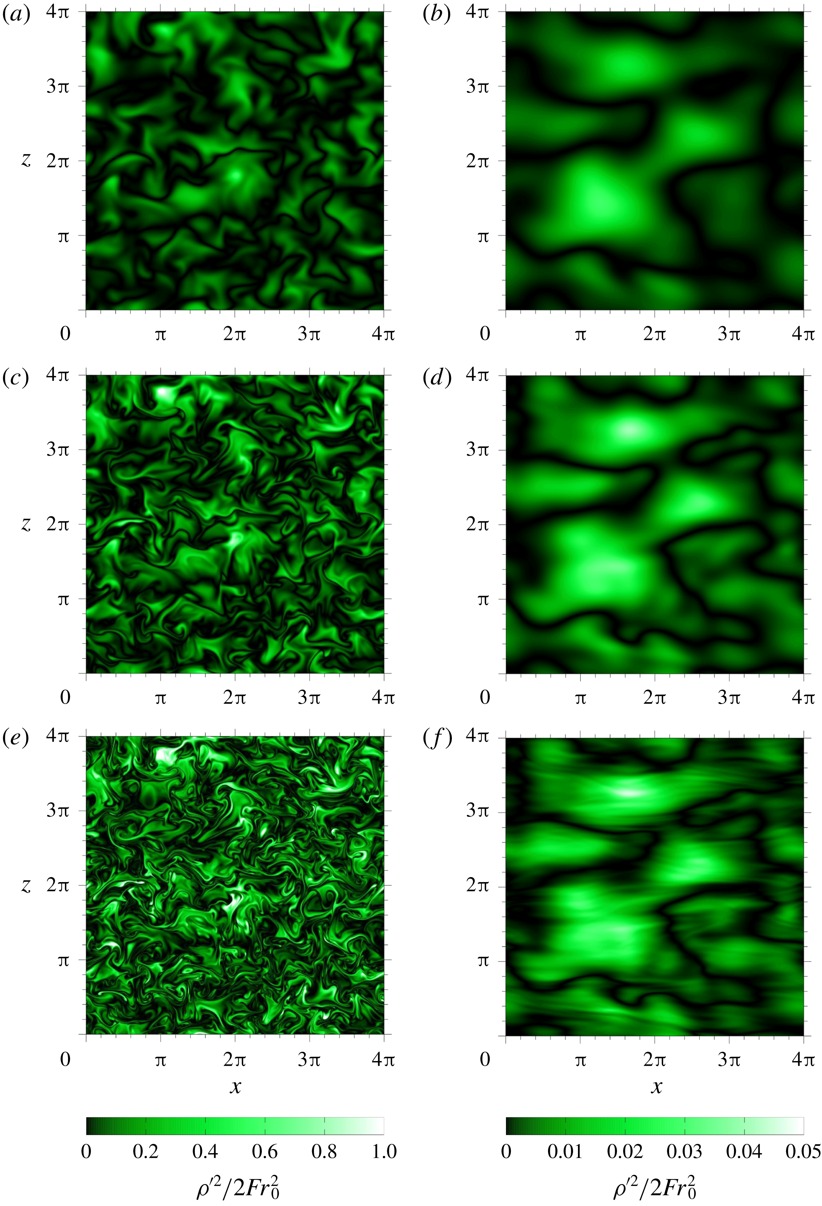
To observe the small-scale structures more clearly, the distributions of potential energy $\unicode[STIX]{x1D70C}^{\prime 2}/(2Fr_{0}^{2})$ in the vertical plane ( $y=0$ ) are presented in colour scale in figure 11, again at $t=4$ and 40. In agreement with figure 9, the potential-energy distribution at $t=4$ is affected significantly by the Prandtl number, and the result for $Pr=70$ (figure 11 e) contains much finer structures than those for lower Prandtl numbers (figures 11 a and 11 c). The structures at $t=40$ are rather independent of $Pr$ (figures 11 b, 11 d and 11 f) since most of the small-scale components below the Kolmogorov scale have decayed (cf. figures 13 c and 13 d). However, similar to the result at $t=4$ (figure 11 e), the vertical structure of the potential energy at high $Pr(=70)$ has components of very small scales, which appear as many thin horizontal streaks in figure 11(f). These streaks correspond to the horizontal wrinkles on the surface of pancakes (figure 10 d). These would be due to the high-vertical-wavenumber components observed in the potential-energy spectra, which will be discussed later (cf. figure 13 d).

Figure 11.

Spatial distributions of the potential energy $\unicode[STIX]{x1D70C}^{\prime 2}/(2Fr_{0}^{2})$ in the vertical plane ( $y=0$ ). The panels show the colour-scale image at: (a)  $Pr=1$ , $t=4$ ; (b)  $Pr=1$ , $t=40$ ; (c)  $Pr=7$ , $t=4$ ; (d)  $Pr=7$ , $t=40$ ; (e)  $Pr=70$ , $t=4$ ; and (f)  $Pr=70$ , $t=40$ .

The agreement between the horizontal scales of the velocity and density perturbations at long time, observed even at a high Prandtl number ( $Pr=70$ ) in figure 10, is identified in figure 12 by the longitudinal Taylor microscales of velocity

(3.4) $$\begin{eqnarray}\unicode[STIX]{x1D706}_{i}^{2}=\overline{u_{i}^{2}}\!\!\left/\,\overline{\left(\frac{\unicode[STIX]{x2202}u_{i}}{\unicode[STIX]{x2202}x_{i}}\right)^{2}},\right.\quad (i=1,2,3),\end{eqnarray}$$

(no summation is taken over the repeated index  $i$ ), and those of density perturbation

(3.5) $$\begin{eqnarray}\unicode[STIX]{x1D706}_{\unicode[STIX]{x1D70C}^{\prime },i}^{2}=\overline{\unicode[STIX]{x1D70C}^{\prime 2}}\!\!\left/\,\overline{\left(\frac{\unicode[STIX]{x2202}\unicode[STIX]{x1D70C}^{\prime }}{\unicode[STIX]{x2202}x_{i}}\right)^{2}},\right.\quad (i=1,2,3),\end{eqnarray}$$

where $\unicode[STIX]{x1D706}_{1}$ and $\unicode[STIX]{x1D706}_{3}$ are associated with the horizontal and vertical scales of velocity, and $\unicode[STIX]{x1D706}_{\unicode[STIX]{x1D70C}^{\prime },1}$ and $\unicode[STIX]{x1D706}_{\unicode[STIX]{x1D70C}^{\prime },3}$ are associated with those of density perturbations (e.g. Riley et al. Reference Riley, Metcalfe, Weissman and West1981). The initial values of $\unicode[STIX]{x1D706}_{1}$ and $\unicode[STIX]{x1D706}_{3}$ are almost equal ( $\unicode[STIX]{x1D706}_{1}=\unicode[STIX]{x1D706}_{3}$ ) since the initial velocity fluctuations are isotropic. However, as time proceeds, the horizontal microscales become larger than the vertical microscales ( $\unicode[STIX]{x1D706}_{1}>\unicode[STIX]{x1D706}_{3}$ and $\unicode[STIX]{x1D706}_{\unicode[STIX]{x1D70C}^{\prime },1}>\unicode[STIX]{x1D706}_{\unicode[STIX]{x1D70C}^{\prime },3}$ ), corresponding to the appearance of the pancake structure in the kinetic and potential-energy distributions (e.g. at $t=40$ , figure 10).

When $Pr=1$ (figure 12 a), the microscales of velocity are nearly equal to those of density perturbation at all times (i.e. $\unicode[STIX]{x1D706}_{1}\simeq \unicode[STIX]{x1D706}_{\unicode[STIX]{x1D70C}^{\prime },1}$ and $\unicode[STIX]{x1D706}_{3}\simeq \unicode[STIX]{x1D706}_{\unicode[STIX]{x1D70C}^{\prime },3}$ ). With the increase of $Pr$ ( $=70$ , figure 12 b), however, the temporal behaviour of the microscales of density perturbation ( $\unicode[STIX]{x1D706}_{\unicode[STIX]{x1D70C}^{\prime },1}$ and $\unicode[STIX]{x1D706}_{\unicode[STIX]{x1D70C}^{\prime },3}$ ) changes significantly, while that of the velocity microscales ( $\unicode[STIX]{x1D706}_{1}$ and $\unicode[STIX]{x1D706}_{3}$ ) changes only a little. Namely, the microscales $\unicode[STIX]{x1D706}_{\unicode[STIX]{x1D70C}^{\prime },1}$ and $\unicode[STIX]{x1D706}_{\unicode[STIX]{x1D70C}^{\prime },3}$ initially decrease significantly due to the initial potential-energy cascade ( $t\lesssim 4$ ), but after that, they increase again, and the horizontal microscale of density perturbation $\unicode[STIX]{x1D706}_{\unicode[STIX]{x1D70C}^{\prime },1}$ becomes almost equal to the horizontal microscale of velocity $\unicode[STIX]{x1D706}_{1}$ at large times ( $t\gtrsim 30$ ). The increase of the vertical microscale $\unicode[STIX]{x1D706}_{\unicode[STIX]{x1D70C}^{\prime },3}$ is not so large, and it is still smaller than the vertical microscale of velocity $\unicode[STIX]{x1D706}_{3}$ at the end of the simulation ( $t=40$ ). These results are consistent with the agreement only in the horizontal scale of the kinetic- and potential-energy distributions at $Pr=70$ (figure 10 c,d).

Figure 12.

Temporal variation of the horizontal and vertical Taylor microscales of velocity and density perturbation for (a)  $Pr=1$ and (b)  $Pr=70$ .

3.3 Energy spectra

We next present the energy spectrum in order to further investigate the small-scale anisotropy of the high- $Pr$ scalar distribution at late times. The horizontal and the vertical spectra of the kinetic energy are defined by

(3.6) $$\begin{eqnarray}E_{K}(k_{H})=\mathop{\sum }_{\substack{ \left|\sqrt{k_{x}^{2}+k_{y}^{2}}-k_{H}\right|<k_{min}/2 \\ k_{z}}}\frac{1}{2}|\hat{u} _{i}(k_{x},k_{y},k_{z})|^{2}\,\frac{1}{k_{min}}\end{eqnarray}$$

and

(3.7) $$\begin{eqnarray}E_{K}(k_{V})=\mathop{\sum }_{\substack{ |k_{z}|=k_{V} \\ k_{x},k_{y}}}\frac{1}{2}|\hat{u} _{i}(k_{x},k_{y},k_{z})|^{2}\,\frac{1}{k_{min}},\end{eqnarray}$$

respectively. Here, $\hat{u} _{i}$ denotes the Fourier component of $u_{i}$ , its argument $(k_{x},k_{y},k_{z})$ is the wavenumber vector, and the minimum wavenumber $k_{min}$ is 0.5 since the side of the computational box is $4\unicode[STIX]{x03C0}$ in the non-dimensional form. Similarly, we define the horizontal and vertical potential-energy spectra as follows:

(3.8) $$\begin{eqnarray}E_{P}(k_{H})=\mathop{\sum }_{\substack{ \left|\sqrt{k_{x}^{2}+k_{y}^{2}}-k_{H}\right|<k_{min}/2 \\ k_{z}}}\frac{1}{2Fr_{0}^{2}}|\hat{\unicode[STIX]{x1D70C}^{\prime }}(k_{x},k_{y},k_{z})|^{2}\,\frac{1}{k_{min}},\end{eqnarray}$$

and

(3.9) $$\begin{eqnarray}E_{P}(k_{V})=\mathop{\sum }_{\substack{ |k_{z}|=k_{V} \\ k_{x},k_{y}}}\frac{1}{2Fr_{0}^{2}}|\hat{\unicode[STIX]{x1D70C}^{\prime }}(k_{x},k_{y},k_{z})|^{2}\,\frac{1}{k_{min}}.\end{eqnarray}$$

The horizontal and vertical spectra of the kinetic and potential energy at $t=4$ and $t=40$ are plotted in figure 13 for all the Prandtl numbers.

At an early time of $t=4$ (figure 13 a,b), the Kolmogorov wavenumber is greater than the Ozmidov wavenumber (i.e. $Re_{b}>1$ ) and the buoyancy does not affect the flow at the Kolmogorov scale. Indeed, the comparison between figures 13(a) and 13(b) shows that the isotropy of the velocity and density perturbations ( $E_{K}(k_{H})\sim E_{K}(k_{V})$ and $E_{P}(k_{H})\sim E_{P}(k_{V})$ at the same $k_{H}$ and $k_{V}$ ) still remains below the Kolmogorov scale. We note also that when $Pr=1$ , i.e. when the Kolmogorov scale and the Batchelor scale agree, the kinetic-energy spectra are almost equal to the potential-energy spectra at high wavenumbers (i.e. $E_{K}(k_{H})=E_{P}(k_{H})$ at $k_{H}\gtrsim k_{K}$ and $E_{K}(k_{V})=E_{P}(k_{V})$ at $k_{V}\gtrsim k_{K}$ ). The potential-energy spectra below the Kolmogorov scale are larger for a larger Prandtl number due to the scalar cascade to a smaller diffusion scale. The kinetic-energy spectra below the Kolmogorov scale also increase with the Prandtl number due to the larger energy conversion from the potential energy by the vertical density flux (cf. figures 3 a,b and 14 a). On the other hand, at large scales ( $k<k_{K}$ ), the difference due to the Prandtl number is small in figure 13(a,b). The $k^{-1}$ power law of the potential-energy spectrum appears at $Pr=70$ for $k_{K}\lesssim k_{H}\lesssim k_{B}$ and $k_{K}\lesssim k_{V}\lesssim k_{B}$ , showing that Batchelor’s theory holds until the buoyancy affects the sub-Kolmogorov scale (i.e. when $k_{O}<k_{K}$ ). The $k_{H}^{-5/3}$ law of the energy spectra, which is observed by the recent high- $Re$ simulations at $Pr=1$ (e.g. Lindborg Reference Lindborg2006; Brethouwer et al. Reference Brethouwer, Billant, Lindborg and Chomaz2007; Bartello & Tobias Reference Bartello and Tobias2013; de Bruyn Kops Reference de Bruyn Kops2015; Maffioli & Davidson Reference Maffioli and Davidson2016), is absent in the present result. This would be due to the low Reynolds number used in this study. The spectra will be observed if the Reynolds number becomes sufficiently large, since the low-wavenumber ( $k<k_{K}$ ) spectra would not be affected significantly by the Prandtl number.

The energy spectra in the final period of decay ( $t=40$ ), i.e. when the Ozmidov wavenumber is far beyond the Kolmogorov wavenumber ( $k_{K}\ll k_{O}$ or $Re_{b}\ll 1$ , cf. figure 7), are presented in figure 13(c,d). In figure 13(c), the horizontal spectra of potential energy $E_{P}(k_{H})$ for $Pr=7$ and 70 decrease significantly at high wavenumbers, compared to the other spectra. These spectral curves approach the curves of kinetic-energy spectra $E_{K}(k_{H})$ since the energy is converted from potential energy to kinetic energy via the vertical density flux. For example, when $Pr=7$ , the two spectral curves of $E_{P}(k_{H})$ and $E_{K}(k_{H})$ almost agree for $k_{K}<k_{H}\lesssim 10$ . The tendency is weaker in the vertical spectra of potential energy $E_{P}(k_{V})$ for $Pr=7$ and 70 (figure 13 d). This corresponds to the Prandtl-number dependence of the potential-energy distributions observed in figures 10 and 11, where the small-scale fluctuations in the vertical direction existed only in the case of $Pr=70$ (figure 10 d) and not in the case of $Pr=1$ (figure 10 b).

Figure 13.

Plots of (a)  $E_{K}(k_{H})$ and $E_{P}(k_{H})$ at $t=4$ , (b)  $E_{K}(k_{V})$ and $E_{P}(k_{V})$ at $t=4$ , (c)  $E_{K}(k_{H})$ and $E_{P}(k_{H})$ at $t=40$ and (d)  $E_{K}(k_{V})$ and $E_{P}(k_{V})$ at $t=40$ , where the four energy spectra $E_{K}(k_{H}),E_{K}(k_{V}),E_{P}(k_{H})$ and $E_{P}(k_{V})$ are defined by (3.6)–(3.9). The Kolmogorov, Ozmidov and Batchelor wavenumbers for $Pr=70$ are indicated by the arrows at the top of each panel.

Figure 14(a) shows the Prandtl-number dependence of the co-spectrum of the vertical density flux

(3.10) $$\begin{eqnarray}C_{\unicode[STIX]{x1D70C}^{\prime }w}(k)=\mathop{\sum }_{\left|\sqrt{k_{x}^{2}+k_{y}^{2}+k_{z}^{2}}-k\right|<k_{min}/2}\frac{1}{Fr_{0}^{2}}\,\text{Re}[\hat{\unicode[STIX]{x1D70C}^{\prime }}(k_{x},k_{y},k_{z}){\hat{w}}^{\ast }(k_{x},k_{y},k_{z})]\,\frac{1}{k_{min}},\end{eqnarray}$$

which satisfies

(3.11) $$\begin{eqnarray}\frac{1}{Fr_{0}^{2}}\overline{\unicode[STIX]{x1D70C}^{\prime }w}=\int _{0}^{\infty }C_{\unicode[STIX]{x1D70C}^{\prime }w}(k)\,\text{d}k,\end{eqnarray}$$

where the asterisk in (3.10) denotes the complex conjugate, and not a dimensional quantity. The co-spectrum at large scales ( $k\lesssim k_{O}$ ) oscillates in time and changes sign, i.e. it is positive when $t=4$ (figure 14 a), while it is negative when $t=6$ . On the other hand, the co-spectrum at wavenumbers larger than the Kolmogorov wavenumber ( $k\gtrsim k_{K}$ ) is persistently negative and counter-gradient, showing that the potential energy is converted continuously into kinetic energy.

The larger potential energy in the small-scale fluctuations of a higher-Prandtl-number scalar would lead to a stronger counter-gradient flux at small scales, so that the vertical density flux $\overline{\unicode[STIX]{x1D70C}^{\prime }w}/Fr_{0}^{2}$ becomes more strongly counter-gradient (figure 3 a). At the same time, the kinetic-energy spectra $E_{K}(k_{H})$ and $E_{K}(k_{V})$ decay more slowly near the Kolmogorov wavenumber (figure 13 a,b).

The same spectral behaviour has been observed in the previous experiments. For example, water channel experiments for salt stratification ( $Pr=700$ ; Komori & Nagata Reference Komori and Nagata1996) showed a strong counter-gradient flux at high wavenumbers. On the other hand, wind tunnel experiments for thermally stratified flow ( $Pr=0.7$ ; Lienhard & Van Atta Reference Lienhard and Van Atta1990) showed a weaker counter-gradient flux at low wavenumbers. In a numerical simulation for two Prandtl numbers ( $Pr=1$ and 2), Gerz & Yamazaki (Reference Gerz and Yamazaki1993) found a persistent counter-gradient flux at high wavenumbers only for $Pr=2$ . Similar Prandtl-number dependence has been obtained by the rapid distortion theory (RDT) (Hanazaki & Hunt Reference Hanazaki and Hunt1996).

Figure 14.

Prandtl-number dependence of (a) the co-spectrum of the vertical density flux, $C_{\unicode[STIX]{x1D70C}^{\prime }w}(k)$ , and (b) dissipation spectra of kinetic and potential energies, $D_{K}(k)$ and $D_{P}(k)$ , in the pre-multiplied form at $t=4$ . The Kolmogorov, Ozmidov and Batchelor wavenumbers for $Pr=70$ are indicated by the arrows at the top of each panel.

In figure 14(b) we show the pre-multiplied spectra of energy dissipation rates at $t=4$ . The dissipation spectra of kinetic energy and potential energy are defined by

(3.12) $$\begin{eqnarray}D_{K}(k)=\mathop{\sum }_{\left|\sqrt{k_{x}^{2}+k_{y}^{2}+k_{z}^{2}}-k\right|<k_{min}/2}\frac{k_{j}^{2}}{Re_{0}}|\hat{u} _{i}(k_{x},k_{y},k_{z})|^{2}\,\frac{1}{k_{min}},\end{eqnarray}$$

and

(3.13) $$\begin{eqnarray}D_{P}(k)=\mathop{\sum }_{\left|\sqrt{k_{x}^{2}+k_{y}^{2}+k_{z}^{2}}-k\right|<k_{min}/2}\frac{k_{j}^{2}}{Pr\,Re_{0}Fr_{0}^{2}}|\hat{\unicode[STIX]{x1D70C}^{\prime }}(k_{x},k_{y},k_{z})|^{2}\,\frac{1}{k_{min}},\end{eqnarray}$$

respectively. The peak wavenumber of kinetic-energy dissipation ( $kD_{K}(k)$ ) shifts only slightly with $Pr$ , while that of potential-energy dissipation ( $kD_{P}(k)$ ) increases significantly with $Pr$ . Figure 14(b) shows also that the peak wavenumber of $kD_{K}(k)$ is close to the Kolmogorov wavenumber  $k_{K}$ , and the peak of $kD_{P}(k)$ is close to the Batchelor wavenumber  $k_{B}$ . The increase of the maximum value of $kD_{K}(k)$ with $Pr$ explains the slight increase of $\unicode[STIX]{x1D716}_{K}$ as already discussed in figure 3(b). A similar trend has been observed in the vorticity spectrum of the turbulent mixing layer (see figures 12 and 13 of Salehipour et al. (Reference Salehipour, Peltier and Mashayek2015)).

We now examine whether the energy spectra obey the well-known scaling laws. The potential-energy spectra normalised by the strain rate at the Kolmogorov scale $(\unicode[STIX]{x1D708}^{\ast }/\unicode[STIX]{x1D716}_{K}^{\ast })^{1/2}$ , the potential-energy dissipation rate $\unicode[STIX]{x1D716}_{P}^{\ast }$ and the scalar diffusion coefficient $\unicode[STIX]{x1D705}^{\ast }$ for $Pr=70$ are shown in figure 15. Note that the Kolmogorov wavenumber normalised by the Batchelor wavenumber is constant in time: $k_{K}^{\ast }/k_{B}^{\ast }=1/\sqrt{70}\simeq 0.12$ . When $t\lesssim 10$ , the spectral collapse onto a single curve at wavenumbers higher than the Batchelor wavenumber and the $k^{-1}$ power law are clearly found in both the horizontal and the vertical spectra as well as the passive scalar spectrum (e.g. Bogucki et al. Reference Bogucki, Domaradzki and Yeung1997; Yeung et al. Reference Yeung, Xu, Donzis and Sreenivasan2004). After $t\sim 10$ , at which the Ozmidov wavenumber exceeds the Kolmogorov wavenumber, the horizontal spectrum begins to decrease in $k_{H}^{\ast }>k_{K}^{\ast }$ and increase in $k_{H}^{\ast }<k_{K}^{\ast }$ , resulting in a very steep spectrum. On the other hand, the Batchelor scaling reasonably holds for the vertical spectrum even after the Ozmidov wavenumber exceeds the Kolmogorov wavenumber ( $t\gtrsim 10$ ); they converge well in $k_{V}^{\ast }>k_{K}^{\ast }$ as shown in figure 15(b). It is also found that the slope around $k_{V}^{\ast }/k_{B}^{\ast }\simeq 5\times 10^{-2}$ becomes steeper as time passes, and eventually approaches  $-3$ .

Figure 15.

Normalised potential-energy spectrum for $Pr=70$ : (a) horizontal spectrum and (b) vertical spectrum. The vertical solid line shows the Kolmogorov wavenumber divided by the Batchelor wavenumber, i.e. $k_{K}^{\ast }/k_{B}^{\ast }=1/\sqrt{70}\simeq 0.12$ .

Figure 16 presents the kinetic-energy spectra for $Pr=70$ normalised by the energy dissipation $\unicode[STIX]{x1D716}_{K}^{\ast }$ and the kinematic viscosity  $\unicode[STIX]{x1D708}^{\ast }$ . The result is similar to the normalised potential-energy spectrum in the sense that the horizontal spectrum deviates from the Kolmogorov scaling when $t\gtrsim 10$ , whereas the vertical spectrum completely collapses onto a single curve. The collapse of the vertical spectrum is also reported by the experiment using a salt-stratified fluid by Praud et al. (Reference Praud, Fincham and Sommeria2005). However, the $k_{V}^{-3}$ power law in the vertical spectrum they observed is not found in figure 16(b) because the Reynolds number is too small to realise such a constant slope in the low-wavenumber range in our simulations. The normalised spectrum of the vertical velocity in salt-stratified water experiments ( $Pr=700$ ) is presented in figure 19 of Itsweire et al. (Reference Itsweire, Helland and Van Atta1986), showing a slight dispersion at $k_{x}^{\ast }/k_{K}^{\ast }\gtrsim 10^{0}$ . Though they attributed the dispersion of the spectra at high wavenumbers to experimental noise, the energy spectrum could actually deviate from the universal curve since the Kolmogorov scale approaches the Ozmidov scale far downstream of the water channel in their experiment (cf. their figures 4 and 8).

Figure 16.

Normalised kinetic-energy spectrum for $Pr=70$ : (a) horizontal spectrum and (b) vertical spectrum. The vertical solid line shows $k_{H}^{\ast }/k_{K}^{\ast }=1$ or $k_{V}^{\ast }/k_{K}^{\ast }=1$ .

3.4 Generation of the vertically thin structures in the density perturbation

In the remainder of this paper, we discuss how the anisotropic distribution of the potential energy at high wavenumbers for high Prandtl numbers is generated. According to Batchelor (Reference Batchelor1959), the scalar fluctuations smaller than the Kolmogorov scale are generated by a straining motion of the fluid at the Kolmogorov scale. Thus, we examine the direction of the principal axes of the strain-rate tensor, which is defined by $\unicode[STIX]{x1D61A}_{ij}=(\unicode[STIX]{x2202}u_{i}/\unicode[STIX]{x2202}x_{j}+\unicode[STIX]{x2202}u_{j}/\unicode[STIX]{x2202}x_{i})/2$ . Since the strain-rate tensor is a real-valued symmetric tensor, it has three principal values ( $\unicode[STIX]{x1D6FC}\geqslant \unicode[STIX]{x1D6FD}\geqslant \unicode[STIX]{x1D6FE}$ ) and the corresponding principal axes ( $\unicode[STIX]{x1D736},\unicode[STIX]{x1D737}$ and $\unicode[STIX]{x1D738}$ ) are orthogonal. The incompressibility condition ( $\unicode[STIX]{x1D6FC}+\unicode[STIX]{x1D6FD}+\unicode[STIX]{x1D6FE}=0$ ) requires $\unicode[STIX]{x1D6FC}>0$ and $\unicode[STIX]{x1D6FE}<0$ . We consider the cosines of the angles between the principal axes and the vertical axis,

(3.14a-c ) $$\begin{eqnarray}\cos \unicode[STIX]{x1D703}_{z\unicode[STIX]{x1D6FC}}=\boldsymbol{e}_{z}\boldsymbol{\cdot }\unicode[STIX]{x1D736},\quad \cos \unicode[STIX]{x1D703}_{z\unicode[STIX]{x1D6FD}}=\boldsymbol{e}_{z}\boldsymbol{\cdot }\unicode[STIX]{x1D737},\quad \cos \unicode[STIX]{x1D703}_{z\unicode[STIX]{x1D6FE}}=\boldsymbol{e}_{z}\boldsymbol{\cdot }\unicode[STIX]{x1D738},\end{eqnarray}$$

and the cosine of the angle between the density gradient and the vertical axis,

(3.15) $$\begin{eqnarray}\cos \unicode[STIX]{x1D703}_{z\unicode[STIX]{x1D70C}^{\prime }}=\boldsymbol{e}_{z}\boldsymbol{\cdot }\frac{\unicode[STIX]{x1D735}\unicode[STIX]{x1D70C}^{\prime }}{|\unicode[STIX]{x1D735}\unicode[STIX]{x1D70C}^{\prime }|},\end{eqnarray}$$

where $\boldsymbol{e}_{z}$ is the unit vector in the vertical direction.

Figure 17(a) presents the probability density functions (p.d.f.s) of $|\text{cos}\,\unicode[STIX]{x1D703}_{z\unicode[STIX]{x1D6FC}}|$ , $|\text{cos}\,\unicode[STIX]{x1D703}_{z\unicode[STIX]{x1D6FD}}|$ , $|\text{cos}\,\unicode[STIX]{x1D703}_{z\unicode[STIX]{x1D6FE}}|$ and $|\text{cos}\,\unicode[STIX]{x1D703}_{z\unicode[STIX]{x1D70C}^{\prime }}|$ for $Pr=70$ at $t=4$ . The highest probability of $|\text{cos}\,\unicode[STIX]{x1D703}_{z\unicode[STIX]{x1D6FC}}|$ and $|\text{cos}\,\unicode[STIX]{x1D703}_{z\unicode[STIX]{x1D6FE}}|$ occurs when $|\text{cos}\,\unicode[STIX]{x1D703}_{z\unicode[STIX]{x1D6FC}}|=1$ (or $\unicode[STIX]{x1D703}_{z\unicode[STIX]{x1D6FC}}=0,\unicode[STIX]{x03C0}$ ) and $|\text{cos}\,\unicode[STIX]{x1D703}_{z\unicode[STIX]{x1D6FE}}|=1$ (or $\unicode[STIX]{x1D703}_{z\unicode[STIX]{x1D6FE}}=0,\unicode[STIX]{x03C0}$ ), respectively, indicating that the most expansive direction ( $\unicode[STIX]{x1D736}$ ) and the most contractive direction ( $\unicode[STIX]{x1D738}$ ) tend to align with the vertical axis probably because of the Brunt–Väisälä oscillation due to the buoyancy. However, $\unicode[STIX]{x1D736}$ and $\unicode[STIX]{x1D738}$ cannot align with the vertical axis at the same time because they are orthogonal. This can be confirmed by the joint p.d.f. of $|\text{cos}\,\unicode[STIX]{x1D703}_{z\unicode[STIX]{x1D6FC}}|$ and $|\text{cos}\,\unicode[STIX]{x1D703}_{z\unicode[STIX]{x1D6FE}}|$ in figure 17(b). There are two local maxima at $(|\text{cos}\,\unicode[STIX]{x1D703}_{z\unicode[STIX]{x1D6FC}}|,|\text{cos}\,\unicode[STIX]{x1D703}_{z\unicode[STIX]{x1D6FE}}|)=(0,1)$ and $(1,0)$ . Also, the probability density of $|\text{cos}\,\unicode[STIX]{x1D703}_{z\unicode[STIX]{x1D6FD}}|$ becomes largest when $|\text{cos}\,\unicode[STIX]{x1D703}_{z\unicode[STIX]{x1D6FD}}|=0$ (or $\unicode[STIX]{x1D703}_{z\unicode[STIX]{x1D6FD}}=\unicode[STIX]{x03C0}/2$ ), as shown in figure 17(a). After all, at an early time of $t=4$ , either the most expansive direction ( $\unicode[STIX]{x1D736}$ ) or the most contractive direction ( $\unicode[STIX]{x1D738}$ ) tends to be along the vertical axis, while the other two principal axes are horizontal. The p.d.f.s of $|\text{cos}\,\unicode[STIX]{x1D703}_{z\unicode[STIX]{x1D6FC}}|$ , $|\text{cos}\,\unicode[STIX]{x1D703}_{z\unicode[STIX]{x1D6FD}}|$ and $|\text{cos}\,\unicode[STIX]{x1D703}_{z\unicode[STIX]{x1D6FE}}|$ are nearly independent of time until the Ozmidov wavenumber approaches the Kolmogorov wavenumber ( $3\lesssim t\lesssim 6$ ). Figure 17(a) also shows that the probability density of $|\text{cos}\,\unicode[STIX]{x1D703}_{z\unicode[STIX]{x1D70C}^{\prime }}|$ becomes highest at $|\text{cos}\,\unicode[STIX]{x1D703}_{z\unicode[STIX]{x1D70C}^{\prime }}|=1$ , indicating that the density gradient $\unicode[STIX]{x1D735}\unicode[STIX]{x1D70C}^{\prime }$ tends to be vertical and the horizontally flat distribution of density begins to be generated.

Figure 17.

(a,c) The p.d.f.s of $|\text{cos}\,\unicode[STIX]{x1D703}_{z\unicode[STIX]{x1D6FC}}|$ , $|\text{cos}\,\unicode[STIX]{x1D703}_{z\unicode[STIX]{x1D6FD}}|$ , $|\text{cos}\,\unicode[STIX]{x1D703}_{z\unicode[STIX]{x1D6FE}}|$ and $|\text{cos}\,\unicode[STIX]{x1D703}_{z\unicode[STIX]{x1D70C}^{\prime }}|$ for $Pr=70$ . (b,d) Joint p.d.f.s of $|\text{cos}\,\unicode[STIX]{x1D703}_{z\unicode[STIX]{x1D6FC}}|$ and $|\text{cos}\,\unicode[STIX]{x1D703}_{z\unicode[STIX]{x1D6FE}}|$ for $Pr=70$ . Time (a,b)  $t=4$ and (c,d)  $t=40$ .

Figure 17(c) shows the p.d.f.s at $t=40$ . The p.d.f.s of $|\text{cos}\,\unicode[STIX]{x1D703}_{z\unicode[STIX]{x1D6FC}}|$ and $|\text{cos}\,\unicode[STIX]{x1D703}_{z\unicode[STIX]{x1D6FE}}|$ have a peak at $|\text{cos}\,\unicode[STIX]{x1D703}_{z\unicode[STIX]{x1D6FC}}|\sim 0.8$ and $|\text{cos}\,\unicode[STIX]{x1D703}_{z\unicode[STIX]{x1D6FE}}|\sim 0.7$ , respectively. The joint p.d.f. of $|\text{cos}\,\unicode[STIX]{x1D703}_{z\unicode[STIX]{x1D6FC}}|$ and $|\text{cos}\,\unicode[STIX]{x1D703}_{z\unicode[STIX]{x1D6FE}}|$ in figure 17(d) displays only one peak at $|\text{cos}\,\unicode[STIX]{x1D703}_{z\unicode[STIX]{x1D6FC}}|\sim |\text{cos}\,\unicode[STIX]{x1D703}_{z\unicode[STIX]{x1D6FE}}|\sim 0.7\sim 1/\sqrt{2}$ , meaning that both the most expansive direction ( $\unicode[STIX]{x1D736}$ ) and the most contractive direction ( $\unicode[STIX]{x1D738}$ ) tend to make an angle of $45^{\circ }$ with the vertical axis. This situation occurs when the vertical shear of the horizontal flow is dominant in the strain-rate tensor (appendix A). The transition to the p.d.f.s corresponding to the vertically sheared horizontal flow takes place when the Ozmidov wavenumber becomes as large as the Kolmogorov wavenumber ( $t\sim 8$ for $Pr=70$ ). Smyth (Reference Smyth1999) also reported that $\unicode[STIX]{x1D736}$ and $\unicode[STIX]{x1D738}$ point at $45^{\circ }$ from the vertical after the stratified shear turbulence triggered by the Kelvin–Helmholtz instability had decayed ( $Re_{b}\rightarrow 1$ ) and the flow exhibits a pancake structure. The p.d.f. of $|\text{cos}\,\unicode[STIX]{x1D703}_{z\unicode[STIX]{x1D70C}^{\prime }}|$ shows that the density gradient tends to direct towards the vertical axis, and the tendency is much more significant compared to the case of $t=4$ .

In order to investigate whether the vertically sheared horizontal flow is dominant at late times in our simulation, we decompose the kinetic-energy dissipation rate into four components:

(3.16) $$\begin{eqnarray}\displaystyle & \!\!\displaystyle \unicode[STIX]{x1D716}_{H,H}=\frac{1}{Re_{0}}\overline{\left(\frac{\unicode[STIX]{x2202}u}{\unicode[STIX]{x2202}x}\right)^{\!2}\!+\left(\frac{\unicode[STIX]{x2202}u}{\unicode[STIX]{x2202}y}\right)^{\!2}\!+\left(\frac{\unicode[STIX]{x2202}v}{\unicode[STIX]{x2202}x}\right)^{\!2}\!+\left(\frac{\unicode[STIX]{x2202}v}{\unicode[STIX]{x2202}y}\right)^{\!2}}\quad \!(horizontal~shear~of~horizontal~flow),\hspace{-8.39996pt} & \displaystyle \nonumber\\ \displaystyle & & \displaystyle\end{eqnarray}$$

(3.17) $$\begin{eqnarray}\displaystyle & \!\!\displaystyle \unicode[STIX]{x1D716}_{H,V}=\frac{1}{Re_{0}}\overline{\left(\frac{\unicode[STIX]{x2202}u}{\unicode[STIX]{x2202}z}\right)^{\!2}\!+\left(\frac{\unicode[STIX]{x2202}v}{\unicode[STIX]{x2202}z}\right)^{\!2}}\quad \!(vertical~shear~of~horizontal~flow), & \displaystyle\end{eqnarray}$$

(3.18) $$\begin{eqnarray}\displaystyle & \!\!\displaystyle \unicode[STIX]{x1D716}_{V,H}=\frac{1}{Re_{0}}\overline{\left(\frac{\unicode[STIX]{x2202}w}{\unicode[STIX]{x2202}x}\right)^{\!2}\!+\left(\frac{\unicode[STIX]{x2202}w}{\unicode[STIX]{x2202}y}\right)^{\!2}}\quad \!(horizontal~shear~of~vertical~flow), & \displaystyle\end{eqnarray}$$

and

(3.19) $$\begin{eqnarray}\unicode[STIX]{x1D716}_{V,V}=\frac{1}{Re_{0}}\overline{\left(\frac{\unicode[STIX]{x2202}w}{\unicode[STIX]{x2202}z}\right)^{\!2}}\quad \!(vertical~shear~of~vertical~flow),\end{eqnarray}$$

where

(3.20) $$\begin{eqnarray}\unicode[STIX]{x1D716}_{K}=\unicode[STIX]{x1D716}_{H,H}+\unicode[STIX]{x1D716}_{H,V}+\unicode[STIX]{x1D716}_{V,H}+\unicode[STIX]{x1D716}_{V,V}.\end{eqnarray}$$

The contribution from the vertical shear of the horizontal flow, $\unicode[STIX]{x1D716}_{H,V}$ , is expected to be dominant at late times of our simulation. Note that it is not equal to the kinetic-energy dissipation rate of the VSHF (vertically sheared horizontal flow) mode (Smith & Waleffe Reference Smith and Waleffe2002) because $\unicode[STIX]{x1D716}_{H,V}$ includes Fourier modes of $k_{H}=\sqrt{k_{x}^{2}+k_{y}^{2}}\neq 0$ . For an isotropic turbulence (Taylor Reference Taylor1935),

(3.21) $$\begin{eqnarray}\overline{\left(\frac{\unicode[STIX]{x2202}u}{\unicode[STIX]{x2202}x}\right)^{2}}=\overline{\left(\frac{\unicode[STIX]{x2202}v}{\unicode[STIX]{x2202}y}\right)^{2}}=\overline{\left(\frac{\unicode[STIX]{x2202}w}{\unicode[STIX]{x2202}z}\right)^{2}}=\frac{1}{15}\overline{\left(\frac{\unicode[STIX]{x2202}u_{i}}{\unicode[STIX]{x2202}x_{j}}\right)^{2}},\end{eqnarray}$$

and

(3.22) $$\begin{eqnarray}\overline{\left(\frac{\unicode[STIX]{x2202}u}{\unicode[STIX]{x2202}y}\right)^{2}}=\overline{\left(\frac{\unicode[STIX]{x2202}u}{\unicode[STIX]{x2202}z}\right)^{2}}=\overline{\left(\frac{\unicode[STIX]{x2202}v}{\unicode[STIX]{x2202}x}\right)^{2}}=\overline{\left(\frac{\unicode[STIX]{x2202}v}{\unicode[STIX]{x2202}z}\right)^{2}}=\overline{\left(\frac{\unicode[STIX]{x2202}w}{\unicode[STIX]{x2202}x}\right)^{2}}=\overline{\left(\frac{\unicode[STIX]{x2202}w}{\unicode[STIX]{x2202}y}\right)^{2}}=\frac{2}{15}\overline{\left(\frac{\unicode[STIX]{x2202}u_{i}}{\unicode[STIX]{x2202}x_{j}}\right)^{2}},\end{eqnarray}$$

lead to

(3.23a-d ) $$\begin{eqnarray}\frac{\unicode[STIX]{x1D716}_{H,H}}{\unicode[STIX]{x1D716}_{K}}=\frac{6}{15},\quad \frac{\unicode[STIX]{x1D716}_{H,V}}{\unicode[STIX]{x1D716}_{K}}=\frac{4}{15},\quad \frac{\unicode[STIX]{x1D716}_{V,H}}{\unicode[STIX]{x1D716}_{K}}=\frac{4}{15},\quad \frac{\unicode[STIX]{x1D716}_{V,V}}{\unicode[STIX]{x1D716}_{K}}=\frac{1}{15}.\end{eqnarray}$$

Temporal variation of these ratios in stratified flow at $Pr=70$ is presented in figure 18(a), illustrating the deviation from their isotropic values. After $t\sim 8$ , $\unicode[STIX]{x1D716}_{H,V}/\unicode[STIX]{x1D716}_{K}$ rapidly increases, and it eventually reaches ${\sim}0.6$ , while $\unicode[STIX]{x1D716}_{H,H}/\unicode[STIX]{x1D716}_{K}$ and $\unicode[STIX]{x1D716}_{V,H}/\unicode[STIX]{x1D716}_{K}$ become significantly smaller than their isotropic values. The salt-stratified experiments by Fincham et al. (Reference Fincham, Maxworthy and Spedding1996) and Praud et al. (Reference Praud, Fincham and Sommeria2005) reported a higher value of $\unicode[STIX]{x1D716}_{H,V}/\unicode[STIX]{x1D716}_{K}\sim 0.9$ . The smaller $\unicode[STIX]{x1D716}_{H,V}/\unicode[STIX]{x1D716}_{K}$ in our simulation would not be due to the low-Prandtl-number effect because $\unicode[STIX]{x1D716}_{H,V}/\unicode[STIX]{x1D716}_{K}$ generally decreases with increasing Prandtl number (figure 18 b). As the previous numerical simulations by Hebert & de Bruyn Kops (Reference Hebert and de Bruyn Kops2006) report the Reynolds-number dependence of $\unicode[STIX]{x1D716}_{H,V}/\unicode[STIX]{x1D716}_{K}$ , in which $\unicode[STIX]{x1D716}_{H,V}/\unicode[STIX]{x1D716}_{K}$ decreases with decreasing Reynolds number at low Reynolds numbers (see their figure 1), the difference in $\unicode[STIX]{x1D716}_{H,V}/\unicode[STIX]{x1D716}_{K}$ might be caused by the small Reynolds number of our simulation.

Figure 18.

(a) Temporal variations of the ratios of $\unicode[STIX]{x1D716}_{H,H},~\unicode[STIX]{x1D716}_{H,V},~\unicode[STIX]{x1D716}_{V,H}$ and $\unicode[STIX]{x1D716}_{V,V}$ to the kinetic-energy dissipation rate $\unicode[STIX]{x1D716}_{K}$ for $Pr=70$ . The horizontal dotted lines indicate the values for isotropic turbulence: $1/15$ , $4/15$ and $6/15$ from below. (b) The $Pr$ dependence of $\unicode[STIX]{x1D716}_{H,V}/\unicode[STIX]{x1D716}_{K}$ .

We next apply an analysis similar to Batchelor (Reference Batchelor1959) to the late stage of decaying stratified turbulence, i.e. after a certain large time $t_{0}$ (typically $t_{0}>20$ ; cf. figure 18) for which the vertically sheared horizontal flow is dominant down to the Kolmogorov scale. A brief review of the theory for a high- $Pr$ passive scalar by Batchelor (Reference Batchelor1959) is given in appendix B. We consider the deformation of a fluid element whose linear dimension is slightly smaller than the Kolmogorov scale, and whose translational velocity is $\boldsymbol{u}_{el}(t)=(u_{el},v_{el},w_{el})$ . New spatial coordinates $\boldsymbol{X}=(X,Y,Z)$ which translate with the fluid element are introduced, but, unlike in Batchelor (Reference Batchelor1959), they do not rotate, so that the $X,~Y$ and $Z$ axes are always parallel to the $x,~y$ and $z$ axes, respectively. Then, the new coordinate axes do not necessarily agree with the principal axes of the strain-rate tensor. Assuming that $\boldsymbol{X}=\boldsymbol{x}$ at $t=t_{0}$ , i.e. the fluid element is initially located at $\boldsymbol{x}=\mathbf{0}$ , the spatial coordinates $\boldsymbol{X}$ are defined by

(3.24) $$\begin{eqnarray}\boldsymbol{X}=\boldsymbol{x}-\int _{t_{0}}^{t}\boldsymbol{u}_{el}(\unicode[STIX]{x1D70F})\,\text{d}\unicode[STIX]{x1D70F}.\end{eqnarray}$$

A new temporal coordinate $T$ , which represents the elapsed time after $t=t_{0}$ , is also introduced, defined by

(3.25) $$\begin{eqnarray}T=t-t_{0}.\end{eqnarray}$$

If we assume that the velocity in the translational coordinates, $(U,V,W)$ , is dominated by vertically sheared horizontal flow, i.e. $(U,V,W)=(S_{X}Z,S_{Y}Z,0)$ , the transport equation of the density perturbation (2.2) becomes

(3.26) $$\begin{eqnarray}\frac{\unicode[STIX]{x2202}\unicode[STIX]{x1D70C}^{\prime }}{\unicode[STIX]{x2202}T}+S_{X}Z\frac{\unicode[STIX]{x2202}\unicode[STIX]{x1D70C}^{\prime }}{\unicode[STIX]{x2202}X}+S_{Y}Z\frac{\unicode[STIX]{x2202}\unicode[STIX]{x1D70C}^{\prime }}{\unicode[STIX]{x2202}Y}=\frac{1}{Re_{0}Pr}\left(\frac{\unicode[STIX]{x2202}^{2}\unicode[STIX]{x1D70C}^{\prime }}{\unicode[STIX]{x2202}X^{2}}+\frac{\unicode[STIX]{x2202}^{2}\unicode[STIX]{x1D70C}^{\prime }}{\unicode[STIX]{x2202}Y^{2}}+\frac{\unicode[STIX]{x2202}^{2}\unicode[STIX]{x1D70C}^{\prime }}{\unicode[STIX]{x2202}Z^{2}}\right)+w_{el}(t_{0}+T),\end{eqnarray}$$

in the frame of reference moving with the fluid element. The detailed derivation of (3.26) is presented in appendix C.

The assumption that the flow at scales smaller than the Kolmogorov scale is dominated by the vertical shear of the horizontal flow at late times is verified again by examining the kinetic-energy dissipation spectrum tensor, which is defined by

(3.27) $$\begin{eqnarray}\unicode[STIX]{x1D60B}_{ij}(k)=\mathop{\sum }_{\left|\sqrt{k_{x}^{2}+k_{y}^{2}+k_{z}^{2}}-k\right|<k_{min}/2}\frac{k_{j}^{2}}{Re_{0}}|\hat{u} _{i}(k_{x},k_{y},k_{z})|^{2}\,\frac{1}{k_{min}},\end{eqnarray}$$

(no summation is taken over the repeated indices $i$ and $j$ ), and satisfies

(3.28) $$\begin{eqnarray}\frac{1}{Re_{0}}\overline{\left(\frac{\unicode[STIX]{x2202}u_{i}}{\unicode[STIX]{x2202}x_{j}}\right)^{2}}=\int _{0}^{\infty }\unicode[STIX]{x1D60B}_{ij}(k)\,\text{d}k.\end{eqnarray}$$

As shown in figure 19, the contributions from the vertical shear of the horizontal flow ( $\unicode[STIX]{x1D60B}_{13}$ and $\unicode[STIX]{x1D60B}_{23}$ ) are greater than the other components at all wavenumbers at $t=40$ for $Pr=70$ , but they are close to $\unicode[STIX]{x1D60B}_{31}$ , $\unicode[STIX]{x1D60B}_{32}$ and $\unicode[STIX]{x1D60B}_{33}$ at $k\sim k_{K}$ , indicating that the assumption of the vertically sheared horizontal flow holds moderately well.

Figure 19.

Kinetic-energy dissipation spectrum tensor, $\unicode[STIX]{x1D60B}_{ij}$ , at $t=40$ for $Pr=70$ . The Kolmogorov, Ozmidov and Batchelor wavenumbers for $Pr=70$ are indicated by the arrows at the top of the panel.

The magnitude of the strain rate $S_{X}~(\simeq S_{Y})$ is estimated from figure 18 as follows:

(3.29) $$\begin{eqnarray}\frac{\unicode[STIX]{x1D716}_{H,V}}{\unicode[STIX]{x1D716}_{K}}=\frac{\overline{(\unicode[STIX]{x2202}u/\unicode[STIX]{x2202}z)^{2}}+\overline{(\unicode[STIX]{x2202}v/\unicode[STIX]{x2202}z)^{2}}}{Re_{0}\unicode[STIX]{x1D716}_{K}}\simeq \frac{2S_{X}^{2}}{Re_{0}\unicode[STIX]{x1D716}_{K}}\simeq 0.5\quad \text{at}~t\gtrsim 20,\end{eqnarray}$$

which gives

(3.30a,b ) $$\begin{eqnarray}|S_{X}|\simeq \frac{1}{2}\sqrt{Re_{0}\unicode[STIX]{x1D716}_{K}}\quad \text{or}\quad |S_{X}^{\ast }|\simeq \frac{1}{2}\sqrt{\frac{\unicode[STIX]{x1D716}_{K}^{\ast }}{\unicode[STIX]{x1D708}^{\ast }}}=\frac{1}{2t_{K}^{\ast }},\end{eqnarray}$$

where $t_{K}^{\ast }$ is the dimensional Kolmogorov time.

If we define the mean shear rate $S$ by

(3.31) $$\begin{eqnarray}S=\left(\frac{\overline{(\unicode[STIX]{x2202}u/\unicode[STIX]{x2202}z)^{2}}+\overline{(\unicode[STIX]{x2202}v/\unicode[STIX]{x2202}z)^{2}}}{2}\right)^{1/2},\end{eqnarray}$$

it would vary in the time scale of

(3.32) $$\begin{eqnarray}t_{S}=-\frac{S}{\text{d}S/\text{d}t}.\end{eqnarray}$$

The time scale $t_{S}$ for the case of $Pr=70$ is plotted with the Kolmogorov time in figure 20, showing that $t_{S}$ is one order of magnitude larger than  $t_{K}$ . Thus, in the following analysis, we assume that the shear rate $(S_{X},S_{Y})$ is steady during the Kolmogorov time. We mention here, however, that a Lagrangian analysis (e.g. Girimaji & Pope Reference Girimaji and Pope1990) is necessary to validate the assumption of steady shearing, since we consider here that the coordinates translate with the fluid element. For isotropic turbulence, Kraichnan’s spectrum, which takes into account the unsteadiness of the strain rates, often fits the previous DNS results (Bogucki et al. Reference Bogucki, Domaradzki and Yeung1997; Smyth Reference Smyth1999) better than Batchelor’s spectrum, which assumes steady straining.

Figure 20.

The evolution of the time scale of change of the mean shear rate $t_{S}$ and the Kolmogorov time $t_{K}$ at $Pr=70$ .

We now seek a solution of (3.26) in the form of

(3.33) $$\begin{eqnarray}\unicode[STIX]{x1D70C}^{\prime }(\boldsymbol{X},T)=A(T)\sin (\boldsymbol{m}(T)\boldsymbol{\cdot }\boldsymbol{X})+\int _{0}^{T}w_{el}(t_{0}+\unicode[STIX]{x1D70F})\,\text{d}\unicode[STIX]{x1D70F},\end{eqnarray}$$

with an initial condition of $A(0)=A_{0}$ and $\boldsymbol{m}(0)=(m_{X0},m_{Y0},m_{Z0})$ . Substitution of (3.33) into (3.26) gives four ordinary differential equations:

(3.34a-c ) $$\begin{eqnarray}\frac{\text{d}m_{X}}{\text{d}T}=0,\quad \frac{\text{d}m_{Y}}{\text{d}T}=0,\quad \frac{\text{d}m_{Z}}{\text{d}T}=-(S_{X}m_{X}+S_{Y}m_{Y}),\end{eqnarray}$$

and

(3.35) $$\begin{eqnarray}\frac{\text{d}A}{\text{d}T}=-\frac{m_{X}^{2}+m_{Y}^{2}+m_{Z}^{2}}{Re_{0}Pr}A,\end{eqnarray}$$

which can be solved as

(3.36a-c ) $$\begin{eqnarray}m_{X}=m_{X0},\quad m_{Y}=m_{Y0},\quad m_{Z}=m_{Z0}-(S_{X}m_{X0}+S_{Y}m_{Y0})T,\end{eqnarray}$$

and

(3.37) $$\begin{eqnarray}\displaystyle A(T) & = & \displaystyle A_{0}\exp \left[-\frac{1}{Re_{0}Pr}\left\{\vphantom{\frac{1}{3}}(m_{X0}^{2}+m_{Y0}^{2}+m_{Z0}^{2})T\right.\right.\nonumber\\ \displaystyle & & \displaystyle \left.\!\left.-\,m_{Z0}(S_{X}m_{X0}+S_{Y}m_{Y0})T^{2}+\frac{1}{3}(S_{X}m_{X0}+S_{Y}m_{Y0})^{2}T^{3}\right\}\right].\end{eqnarray}$$

Invariance of the horizontal wavenumbers $m_{X}$ and $m_{Y}$ indicates that the vertically sheared horizontal flow does not alter the horizontal scale of density perturbation. The vertical wavenumber $m_{Z}$ increases linearly with time, and the increase during the Kolmogorov time $t_{K}$ can be estimated using (3.30) and (3.36) as

(3.38) $$\begin{eqnarray}|\unicode[STIX]{x0394}m_{Z}|=|m_{Z}(t_{K})-m_{Z0}|=|S_{X}m_{X0}+S_{Y}m_{Y0}|t_{K}\lesssim \frac{|m_{X0}|+|m_{Y0}|}{2}\simeq |m_{X0}|.\end{eqnarray}$$

This would not be large when the flow has a large horizontal scale. Then, the wavenumber vector $\boldsymbol{m}$ would become aligned with the vertical axis slowly if observed in the Kolmogorov time scale, and the density gradient finally directs upwards (cf. figure 17 c). The increase of the vertical wavenumber of fluid elements would explain why the vertical spectrum of potential energy $E_{P}(k_{V})$ below the Kolmogorov scale becomes larger than the horizontal spectrum $E_{P}(k_{H})$ at late times, as observed in figure 15.

We note that the second term on the right-hand side of (3.33) shows the variation of density perturbation due to the vertical movement of the fluid element. The density perturbation increases (or decreases) when the vertical velocity of the fluid element is positive (or negative), since the background density field is stably stratified. However, this term is a function of only $T$ (and  $t_{0}$ ) and is independent of  $\boldsymbol{X}$ , and adds the same density perturbation to every point in the fluid. Therefore, it has no dynamical effects.

In the present numerical simulation, the small-scale vertical structure of the potential energy has been observed only at the highest Prandtl number ( $Pr=70$ ), but has not been observed at lower Prandtl numbers ( $Pr=1$ and 7; cf. figures 10 and 11). The reason would be explained by (3.37), considering a fluid element with an initial disturbance of wavenumber $|\boldsymbol{m}(0)|=\unicode[STIX]{x1D6FC}k_{K}$ , where $\unicode[STIX]{x1D6FC}$ is a constant of order unity. The amplitude decay during the Kolmogorov time can be estimated from (3.37) as

(3.39) $$\begin{eqnarray}\frac{A(t_{K})}{A_{0}}\simeq \exp \left(-\frac{\unicode[STIX]{x1D6FC}^{2}k_{K}^{2}t_{K}}{Re_{0}Pr}\right)=\exp \left(-\frac{\unicode[STIX]{x1D6FC}^{2}}{Pr}\right).\end{eqnarray}$$

If the Prandtl number is not large ( $Pr=O(\unicode[STIX]{x1D6FC}^{2})=O(1)$ ), the density perturbation decreases to $1/\text{e}$ of its initial value during the Kolmogorov time. This means that the density perturbations would decay before the vertically small-scale density distribution is generated in a time typically much longer than $t_{K}$ . When the vertically small-scale components are generated in the density perturbation, corresponding small-scale components of velocity would be generated through the vertical density flux. However, the latter components would also decay in the Kolmogorov time, and will not affect the vertical scale of the velocity perturbation.

The present form of solution is very similar to the previous result by the RDT, which takes into account the initial condition (Hanazaki & Hunt Reference Hanazaki and Hunt2004). The main differences are that the present result is intended for a small-scale phenomenon near the Kolmogorov scale, and the Prandtl number is not limited to $Pr=1$ . Both results show, however, that the temporal variation of wavenumber vector $\boldsymbol{m}(T)$ and the amplitude of perturbation $A(T)$ are determined only by the shear (cf. Townsend Reference Townsend1976), and irrelevant to the stratification even when the scalar is buoyant. The present results indeed reduce to equations (2.6) and (4.4) of Hanazaki & Hunt (Reference Hanazaki and Hunt2004), under the condition of $Pr=1$ and $S_{Y}=0$ .

We finally mention that the nonlinear advection terms in the Navier–Stokes equations and the density equation vanish for the vertically sheared horizontal flow, and such a flow is governed exactly by the linear equations (Majda & Grote Reference Majda and Grote1997). Therefore, the flow dominated by the vertically sheared horizontal flow would be described well by the linear theory.