1 Introduction
Multiple cylindrical structures are widely encountered in engineering, e.g. chimney stacks, chemical reaction towers, offshore structures, bridge piers, bridge decks and skyscrapers in modern cities. The understanding of flow around these structures is both fundamentally and practically of importance. Two slender cylinders of either circular or square cross-section in a staggered, tandem or side-by-side arrangement can be considered as the simplest configurations of these structures. Yet flow around even these simplest of configurations is highly complicated, involving almost all of the important issues of flow around more cylindrical structures such as shear layer interaction, vortex dynamics, flow interference, wake galloping, vortex-induced vibration, resonance, noise generation, etc. Naturally, knowledge of the two-cylinder wake provides important insight into the physics behind more cylindrical structures.
Extensive investigations have been conducted on the wake of two staggered circular cylinders (e.g. Igarashi Reference Igarashi1981; Price & Paıdoussis Reference Price and Paıdoussis1984; Sumner, Price & Paidoussis Reference Sumner, Price and Paidoussis2000; Hu & Zhou Reference Hu and Zhou2008; Sumner Reference Sumner2010); our understanding of this flow has been improved tremendously. A number of flow classifications have been proposed. Kiya et al. (Reference Kiya, Arie, Tamura and Mori1980) measured, at a Reynolds number
 $Re=1.58\times 10^{4}$
based on the free-stream velocity
 $(U_{\infty })$
and the cylinder diameter/width
 $(d)$
, the Strouhal number
 $St$
in the wake of two staggered circular cylinders for a centre-to-centre spacing ratio
 $P^{\ast }=1{-}5$
and a flow incidence angle
 ${\it\alpha}=0{-}90^{\circ }$
with respect to the line connecting the cylinder centres. An asterisk denotes normalization by
 $U_{\infty }$
and/or
 $d$
in this paper. Depending on how
 $St$
behaved compared with its counterpart
 $St_{0}$
in an isolated cylinder wake, they divided the
 $P^{\ast }\text{-}{\it\alpha}$
plane into five regions, i.e. (a)
 $St>St_{0}$
, (b)
 $St<St_{0}$
, (c) bi-stable flow, (d) single-body flow, and (e) weak or no vortex shedding. Zdravkovich (Reference Zdravkovich1987) classified the two-cylinder wake into four regimes: (i) the proximity interference, (ii) wake interference, (iii) proximity–wake interference, and (iv) non-interference regimes. Gu & Sun (Reference Gu and Sun1999) further divided the proximity–wake interference regime into three, i.e. the wake interference, shear layer interference and proximity interference based on cylinder surface pressure data obtained at
 $Re=2.2\times 10^{5}{-}3.3\times 10^{5}$
. Based on extensive laser-induced fluorescence (LIF) flow visualization and particle image velocimetry (PIV) measurements
 $(Re=850{-}1.9\times 10^{3})$
, Sumner et al. (Reference Sumner, Price and Paidoussis2000) divided the flow into single bluff body, small
 ${\it\alpha}$
and large
 ${\it\alpha}$
groups, with a total of nine flow patterns identified in the near wake. Hu & Zhou (Reference Hu and Zhou2008) measured the flow over
 $x^{\ast }=2.5{-}20$
using hot-wire, LIF and PIV techniques at
 $P^{\ast }=1.2{-}4.0$
and
 ${\it\alpha}=0^{\circ }{-}90^{\circ }\,(Re=7.0\times 10^{3})$
. Four distinct flow modes were identified based on the salient features of the vortex streets and their downstream evolution, i.e. two single-street modes S-I and S-II and two twin-street modes T-I and T-II. Mode S-I was further divided into S-Ia and S-Ib in view of their distinct vortex strengths. The dependence of the flow modes on
 $P^{\ast }$
and
 ${\it\alpha}$
is appreciably affected by
 $Re$
(Zhou et al.
Reference Zhou, Feng, Alam and Bai2009; Wong et al.
Reference Wong, Zhou, Alam and Zhou2014).
A great deal of attention has also been given to the flow classification of the special cases, i.e.
 ${\it\alpha}=0^{\circ }$
and
 ${\it\alpha}=90^{\circ }$
. Igarashi (Reference Igarashi1981, Reference Igarashi1984) and Zdravkovich (Reference Zdravkovich1987) proposed three flow regimes for
 ${\it\alpha}=0^{\circ }$
(
 $Re=1.0\times 10^{4}{-}6.5\times 10^{4}$
): (i) the extended body at
 $1.0<P^{\ast }<1.2{-}1.8$
, (ii) the reattachment at
 $1.2{-}1.8<P^{\ast }<3.4{-}3.8$
and (iii) the co-shedding at
 $P^{\ast }>3.8$
. Xu & Zhou (Reference Xu and Zhou2004) examined the
 $Re$
effect on the flow classification of this flow
 $(Re=0.8\times 10^{3}{-}4.2\times 10^{4})$
and further divided the reattachment regime into two subregimes, i.e.
 $P^{\ast }=2.0{-}3.0$
and
 $P^{\ast }=3.0{-}5.0$
, corresponding to the occurrence of shear layer reattachment on the leeward and windward sides of the downstream cylinder, respectively. The two subregimes exhibit distinct flow features (Zhou & Yiu Reference Zhou and Yiu2006). Zdravkovich (Reference Zdravkovich1987) classified the wake of two side-by-side cylinders
 $({\it\alpha}=90^{\circ })$
into three regimes: (i) the single vortex street at
 $P^{\ast }<1.1{-}1.2$
, (ii) the biased gap flow at
 $1.2<P^{\ast }<2.0{-}2.2$
and (iii) the coupled vortex streets at
 $2.7<P^{\ast }<4.0{-}5.0$
. The borders between the regimes are dependent on
 $Re$
(Xu, Zhou & So Reference Xu, Zhou and So2003).
While the circular cylinder represents one category of bluff bodies with continuous and finite curvature, the square cylinder is another representative model for bluff bodies with sharp corners of infinitely large curvature. Furthermore, cylindrical structures of square cross-section are also widely used in engineering. However, the wake of two staggered square cylinders has been given much less attention than that of circular cylinders in the literature. Based on the
 $St$
data over
 $Re=2.76{-}5.52\times 10^{4}$
, Sakamoto, Haniu & Obata (Reference Sakamoto, Haniu and Obata1987) divided the wake of two tandem square cylinders into three regimes. In Regime I
 $(P^{\ast }<4.0)$
, vortices were shed only from the downstream cylinder. Regime II took place at
 $4.0<P^{\ast }<28.0$
, where the arrival of the upstream-cylinder-generated vortices triggered vortex shedding from the downstream cylinder. Regime III corresponded to
 $P^{\ast }>28.0$
at which the two cylinders generated vortices rather independently but the frequency of vortex shedding from the downstream cylinder is lower than that from the upstream. The critical spacing
 $P_{cri}^{\ast }$
between Regimes I and II was found to decrease with increased free-stream turbulence intensity (Sakamoto & Haniu Reference Sakamoto and Haniu1988a
,
 $Re=3.32\times 10^{4}$
). Kim et al. (Reference Kim, Kim, Yoon and Lee2008) examined the flow structure at
 $P^{\ast }<P_{cri}^{\ast }$
and
 $P^{\ast }>P_{cri}^{\ast }$
based on the PIV data measured at
 $Re=5.3\times 10^{3}{-}1.6\times 10^{4}$
. Liu & Chen (Reference Liu and Chen2002) observed at
 $Re=2.0\times 10^{3}{-}1.6\times 10^{4}$
a hysteresis phenomenon in
 $P_{cri}^{\ast }$
when increasing and then decreasing
 $P^{\ast }$
progressively.
Attention has also been given to the wake of two side-by-side square cylinders. Kolar, Lyn & Rodi (Reference Kolar, Lyn and Rodi1997) measured this flow at
 $P^{\ast }=3.0~(Re=2.31\times 10^{4})$
using a two-component laser Doppler anemometer (LDA). Using the lattice Boltzmann method (LBM), Agrawal, Djenidi & Antonia (Reference Agrawal, Djenidi and Antonia2006) observed numerically a biased gap flow between the cylinders at
 $P^{\ast }=1.7$
and a predominant in-phase vortex shedding at
 $P^{\ast }=3.5~(Re=73)$
. Similar work based on LBM simulation was done by Rao, Ni & Liu (Reference Rao, Ni and Liu2008) for
 $P^{\ast }<2.5$
and
 $P^{\ast }>2.5~(Re=73{-}200)$
. Sau, Hsu & Ou (Reference Sau, Hsu and Ou2007) studied numerically at
 $Re=100$
three-dimensional vortices for three groups of
 $P^{\ast }$
, namely,
 $P^{\ast }=1.2{-}1.7$
, 2.7 and 3.1. Recently, Alam, Zhou & Wang (Reference Alam, Zhou and Wang2011) conducted a systematic study on this flow over
 $1.02<P^{\ast }<6.00\,(Re=4.7\times 10^{4})$
and identified four flow regimes, each characterized by distinct flow structures, Strouhal numbers and fluid forces. In the single-body regime or regime A
 $(P^{\ast }<1.3)$
, the shear layers separating alternately from the outer sides of the two cylinders form a single Kármán vortex street and
 $St$
is approximately one half of that behind a single isolated cylinder. At
 $P^{\ast }=1.3{-}2.2$
, the gap flow between the two cylinders is biased, dividing the wake into one narrow and one wide street, corresponding to high and low vortex frequencies, respectively, thus referred to as the two-frequency regime or regime B. A transition regime or regime C occurs at
 $P^{\ast }=2.2{-}3.0$
, where the two-frequency shedding mode changes intermittently to the coupled vortex shedding mode. As a result, three distinct vortex frequencies take place. In the coupled vortex shedding regime or regime D, vortices are separated from the two cylinders at the same frequency. The two streets are predominantly antiphased at
 $P^{\ast }=3.0{-}4.6$
but can be antiphased or inphased at
 $P^{\ast }=4.6{-}6.0$
. They further found that this flow displays a marked difference in many facets, from flow classification to fluid forces from that behind two side-by-side circular cylinders, which is linked to the distinct flow separation natures between the two types of cylinders. A difference between their gap passage geometries and gap flows is also a crucial contributor to the observed difference.
There has been so far no systematic investigation of the wake of two staggered square cylinders. One may surmise, based on Alam et al.’s (Reference Alam, Zhou and Wang2011) finding, that this wake must be different in many aspects from its circular cylinder counterpart. Furthermore, flow patterns around two staggered square cylinders should be sensitive to the incidence angle
 ${\it\alpha}$
in view of the fact that flow around an isolated square prism is highly sensitive to
 ${\it\alpha}$
(e.g. Igarashi Reference Igarashi1984; Yoon, Yang & Choi Reference Yoon, Yang and Choi2010). Then, how should the flow be classified? The effect of the separation point, gap passage geometry and gap flow on the other aspects of the flow can be fascinating, such as interference between cylinders, shedding frequencies and individual streets. This work aims to address the above issues based on extensive hot-wire, LIF flow visualization and PIV measurements in the wake of two staggered cylinders. The dependence on
 $P^{\ast }$
and
 ${\it\alpha}$
of
 $St$
, shear layer interaction, flow structure and their downstream evolution are examined in detail.
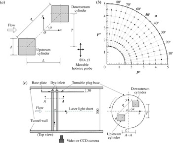
(a) Experimental arrangement. The hot-wire measurement was conducted at
 $x^{\ast }=4,7,10,15$
and
 $y^{\ast }=0,\pm 1,\pm 2,\pm 3,\pm 4,\pm 5$
for each
 $x^{\ast }$
. (b) Measurement positions and techniques: ○, hot-wire; ●, hot-wire and PIV measurement. (c) Experimental set-up of PIV (not in scale, units in mm).

2 Experimental details
Measurements are conducted in a low-speed closed-circuit wind tunnel with a test section of
 $0.6~\text{m}\times 0.6~\text{m}$
cross-section and 2.4 m in length. See Zhou & Yiu (Reference Zhou and Yiu2006) for more details on this tunnel. Figure 1 shows schematically experimental arrangement, along with the definitions of
 $P$
,
 ${\it\alpha}$
,
 $L$
and
 $T$
and the coordinate system of
 $x$
,
 $y$
and
 $z$
, whose origin is defined at the midpoint of the line connecting the cylinder centres. Two identical aluminium square cylinders of
 $d=19~\text{mm}$
, placed at 0.3 m downstream of the tunnel contraction section, are mounted symmetrically about the horizontal midplane (
 $x$
–
 $z$
plane) and spanned the entire width of the test section, resulting in an aspect ratio of 31.6 and a maximum blockage ratio of 6.3 %. The blockage ratio is small enough and no correction is made for measurements (West & Apelt Reference West and Apelt1982; Farrel & Blessmann Reference Farrel and Blessmann1983; Alam & Zhou Reference Alam and Zhou2007), while the aspect ratio is adequately large to neglect the end effect of the cylinders. The square cylinders are made hollow, with a wall thickness of 3 mm and the radius of their corners was 0.5 mm, or
 $0.026d$
. This slightly rounded corner should not have any appreciable effect on the wake (Hu, Zhou & Dalton Reference Hu, Zhou and Dalton2006). A total of 152 configurations of cylinders are investigated, where
 $P^{\ast }$
varies from 1.5 to 5.0, with an increment of 0.5, and
 ${\it\alpha}$
varies from
 $0^{\circ }$
to
 $90^{\circ }$
, with a
 $5^{\circ }$
increment (figure 1
b). The minimum gap between the cylinders is approximately
 $0.1d$
at
 $P^{\ast }=1.5$
and
 ${\it\alpha}=45^{\circ }$
. For each configuration, the upper side surfaces of both cylinders are checked using a foot level to ensure they are aligned with the incident flow. The angular resolution is
 $\pm 0.5^{\circ }$
. Measurements are conducted at
 $U_{\infty }=10~\text{m}~\text{s}^{-1}$
, corresponding to
 $Re=1.3\times 10^{4}$
. The turbulence intensity
 $T_{u}$
is less than 0.5 % in the absence of the cylinders.
A hot-wire probe (55P11, Dantec), mounted on a three-dimensional (3-D) computer-controlled traversing mechanism (figure 1
a) is used to measure the streamwise fluctuating velocity
 $(u)$
at
 $x^{\ast }=4{-}15$
and
 $y^{\ast }=0{-}\pm 5$
. The hot-wire signal is low-pass filtered at 1 kHz and sampled at 2.5 kHz using a 16-channel A/D board (NI PCI-6143). The sampling duration is 20 s for each record. The power spectrum density function,
 $E_{u}$
, of
 $u$
is calculated using a fast Fourier transform (FFT) algorithm. The frequency resolution in
 $E_{u}$
is estimated to be approximately 1.95 Hz based on the FFT window width and sampling frequency (Zhou et al.
Reference Zhou, Du, Mi and Wang2012), resulting in an uncertainty of approximately
 $\pm 3\,\%$
in
 $St$
in an isolated single cylinder wake, which acts as a reference for comparison. In this work,
 $St$
is defined as the normalized frequency of predominant vortices measured at a given
 $x^{\ast }$
, not necessarily vortices shed from the cylinders. Unlike a single-cylinder wake,
 $St$
may vary rapidly behind two staggered cylinders. In general,
 $St$
captured at
 $x^{\ast }=4$
corresponds to the frequencies of vortex shedding from the cylinders, but not necessarily so if measured downstream (
 $x^{\ast }=7$
, 10 and 15).
The flow structure is captured using a Dantec PIV2100 system at
 $Re=1.3\times 10^{4}$
for a number of representative configurations (figure 1
b), as identified from hot-wire measurements, in a closed-loop water tunnel. The working section of the tunnel is 2 m long, 0.3 m wide and 0.6 m high, with a speed range of
 $0.02{-}4.00~\text{m}~\text{s}^{-1}$
. Please see Wang & Zhou (Reference Wang and Zhou2009) for more details of this tunnel. Figure 1(c) shows schematically the experimental set-up. The two cylinders, identical to those used in the hot-wire measurement, are cantilever supported by a turntable plug base fitted to a vertical base plate. The free ends of the cylinders reach the tunnel wall. The maximum blockage by the two cylinders is the same (6.3 %) as in the wind tunnel, though the cylinder aspect ratio (14.2) is smaller, which exceeds the critical value (10) for the assumption of an infinite cylinder (West & Apelt Reference West and Apelt1993). The aspect ratio effect is, therefore, negligible. Flow is seeded uniformly with particles of a spherical shape and approximately 10 microns in diameter. The capture of particle images by a CCD camera (HiSense MkII, gain
 $\times$
4, double frames,
 $1344\times 1024$
pixels) placed perpendicularly to the laser light sheet plane (figure 1
c) is synchronized with the laser illumination by a Dantec Flowmap processor. Details of the calculation algorithm can be found in Raffel, Willert & Kompenhans (Reference Raffel, Willert and Kompenhans1998). A total of 1271 velocity vectors
 $(41\times 31)$
are obtained, with the vector spacing being approximately
 $0.37d$
, producing the same number of spanwise vorticity
 ${\it\omega}_{z}^{\ast }\,(={\it\omega}_{z}d/U_{\infty })$
. Uncertainties in velocity and vorticity are estimated to be 3 % and 5 %, respectively.
The LIF flow visualization
 $(Re=1.3\times 10^{4})$
is conducted in the wind tunnel introduced above. The cylinders are painted black to minimize light reflection. Smoke with a particle size of
 $1~{\rm\mu}\text{m}$
in diameter, generated from paraffin oil, is released from two rows of pinholes, 0.7 mm in diameter and 1-mm in separation, drilled 9 mm away from the nominal forward stagnation line of both cylinders (hollow). The flow images are illuminated and captured using the same laser source and CCD camera as in the PIV measurements.
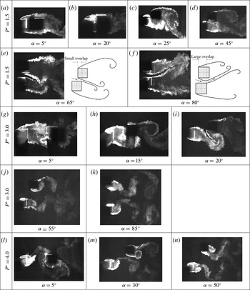
Typical flow structures from LIF flow visualization for various configurations of
 $(P^{\ast },{\it\alpha})$
.
 $Re=1.3\times 10^{4}$
. Flow is left to right.

3 Typical flow structures
Flow around two cylinders depends strongly on
 $P^{\ast }$
and
 ${\it\alpha}$
. An overview of this dependence is crucial for understanding the flow. At small
 $P^{\ast }$
such as 1.5, the two shear layers separating from the leading corners of the upstream cylinder reattach on the side surfaces of the downstream cylinder at
 ${\it\alpha}=0^{\circ }$
(not shown), but only the upper (inner) shear layer reattaches as
 ${\it\alpha}$
is increased to
 $5^{\circ }$
(figure 2
a). Vortex shedding takes place only behind the downstream cylinder, generating a single vortex street. At
 ${\it\alpha}=20^{\circ }$
, the shear layer reattaches the surfaces around the upper leading corner (figure 2
b). A further increase in
 ${\it\alpha}$
results in reattachment on the front surface (
 ${\it\alpha}=25^{\circ }$
, figure 2
c). As
 ${\it\alpha}$
reaches
 $45^{\circ }$
(figure 2
d), the shear layer fails to reattach, passing through the gap as squeezed by the shear layer separating from the lower (inner) leading corner of the downstream cylinder. The two inner shear layers with a small lateral separation are very weak and do not appear to roll up or interact with the outer shear layers. Again, a single street is generated behind the cylinders. A large
 ${\it\alpha}\,(=65^{\circ })$
allows a gap flow growth in thickness and the two inner shear layers gain strength to roll up oppositely, forming vortices (figure 2
e). The two inner cylinder surfaces form effectively a nozzle, and the gap flow looks like a jet, biased toward the upstream cylinder, thus dividing the wake into a narrow and a wide street behind the upstream and downstream cylinders, respectively. See the sketch in figure 2(e). When
 ${\it\alpha}$
is further enlarged, exceeding
 $70^{\circ }$
, the ‘nozzle’ increases in length and width, the gap flow is first directed downward, hitting the upper surface of the upstream cylinder and then bouncing back upward (figure 2
f), which is presently referred to as the hit-and-bounce phenomenon. As a result, the narrow street occurs behind the downstream cylinder, observed for the first time. The observation is interesting and in distinct contrast to that in the wake of two staggered circular cylinders, where the gap flow is always biased toward the upstream cylinder (e.g. Sumner et al.
Reference Sumner, Price and Paidoussis2000; Alam, Sakamoto & Zhou Reference Alam, Sakamoto and Zhou2005; Hu & Zhou Reference Hu and Zhou2008). It is the combined effect of the fixed separation point and the infinitely large curvature radius of the cylinder surface that produces the gap flow biased toward the downstream cylinder. At
 ${\it\alpha}=90^{\circ }$
, the gap flow can be biased upward or downward (Alam et al.
Reference Alam, Zhou and Wang2011).
At
 $P^{\ast }=3.0$
both upper and lower shear layers reattach on the side surfaces of the downstream cylinder at
 ${\it\alpha}=0^{\circ }$
(not shown), but only the upper shear layer reattaches on the upper surface, near the leading corner, of the downstream cylinder at
 ${\it\alpha}=5^{\circ }$
(figure 2
g) and impinges upon the front surface at
 ${\it\alpha}=15^{\circ }$
(figure 2
h). For
 ${\it\alpha}=20^{\circ }{-}80^{\circ }$
(figure 2
i,j), the shear layer is biased, without reattachment, toward the upstream cylinder, resulting in a narrow and a wide street. At
 ${\it\alpha}>80^{\circ }$
, the wake consists of two coupled streets of the same width, either inphased or antiphased (figure 2
k).
Once
 $P^{\ast }\geqslant 4$
, the shear layers separated from the upstream cylinder roll up, forming vortices, in the gap between the cylinders. The vortices impinge on the downstream cylinder at a very small
 ${\it\alpha}$
(
 ${<}\,15^{\circ }$
, figure 2
l) or interact with the lower shear layer or vortices associated with the downstream cylinder at
 ${\it\alpha}=15^{\circ }{-}30^{\circ }$
(figure 2
m). For
 $30^{\circ }<{\it\alpha}<70^{\circ }$
, being laterally further away from each other, the two streets appear to be interacting weakly (figure 2
n). The street behind the upstream cylinder is narrower than the other, as will be confirmed from
 $St$
and PIV data.
4 Strouhal numbers
4.1 Tandem and side-by-side arrangements
There have been quite a few reports on
 $St$
in the wake of two tandem
 $({\it\alpha}=0^{\circ })$
or side-by-side
 $({\it\alpha}=90^{\circ })$
cylinders. The present data, including
 $St_{0}$
measured in an isolated cylinder wake
 $(Re=1.3\times 10^{4})$
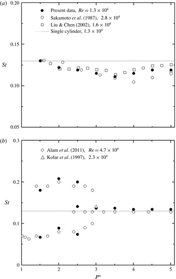
, are compared with those previously reported in figure 3. The present
 $St_{0}\,(=0.134)$
agrees well with those reported in the literature (e.g. Vickery Reference Vickery1966; Norberg Reference Norberg1993; Zhou & Antonia Reference Zhou and Antonia1994). So do those for
 ${\it\alpha}=0^{\circ }$
and
 $90^{\circ }$
(figure 3).
Variations in
 $St$
with
 $P^{\ast }$
: (a) tandem
 $({\it\alpha}=0^{\circ })$
and (b) side-by-side
 $({\it\alpha}=90^{\circ })$
arrangements. Present data were measured at
 $(x^{\ast },y^{\ast })=(4,-4)$
and (4, 4).

At
 ${\it\alpha}=0^{\circ }$
, the
 $St$
drops slowly until
 $P^{\ast }=3.5$
and then rises gradually, approaching
 $St_{0}$
, as
 $P^{\ast }$
increases (figure 3
a). It may be inferred that the critical spacing
 $P_{cri}^{\ast }$
for transition from reattachment to the co-shedding regime is presently between 3.5 and 4.0 (Liu & Chen Reference Liu and Chen2002), slightly deviating from Sakamoto et al.’s (Reference Sakamoto, Haniu and Obata1987) estimate
 $(P_{cri}^{\ast }=4.0)$
. The deviation is ascribed to different experimental conditions. The present
 $Re$
, blockage ratio and
 $T_{u}$
are
 $1.3\times 10^{4}$
, 6.3 % and 0.5 %, respectively, compared with
 $5.52\times 10^{4}$
, 9.8 % and 0.19 % in Sakamoto et al.’s (Reference Sakamoto, Haniu and Obata1987) measurements. In general, a larger blockage ratio and a smaller
 $T_{u}$
result in a longer vortex formation length (Lee Reference Lee1975; West & Apelt Reference West and Apelt1982; Zdravkovich Reference Zdravkovich1997) and hence a larger
 $P_{cri}^{\ast }$
, as seen from Sakamoto et al.’s (Reference Sakamoto, Haniu and Obata1987) data. Sakamoto & Haniu (Reference Sakamoto and Haniu1988a
) conducted an experiment on the effect of
 $T_{u}$
on the wake of two tandem square cylinders and observed that an increased
 $T_{u}$
led to a smaller
 $P_{cri}^{\ast }$
, for example,
 $P_{cri}^{\ast }=4.0$
for
 $T_{u}<0.19\,\%$
but
 $P_{cri}^{\ast }=3.2{-}4.0$
for
 $T_{u}=1.4\,\%$
.
At
 ${\it\alpha}=90^{\circ }$
(figure 3
b), one single and two distinct
 $St$
are captured at
 $P^{\ast }<1.3$
and
 $1.3<P^{\ast }<2.2$
, respectively. The former occurs when the two cylinders of small
 $P^{\ast }$
act as a single body and the shear layers separate alternately from the free-stream sides of the cylinders, producing a single Kármán vortex street. On the other hand, the latter is associated with a narrow and a wide street behind the cylinders (Zdravkovich Reference Zdravkovich1987; Alam, Moriya & Sakamoto Reference Alam, Moriya and Sakamoto2003a
; Alam et al.
Reference Alam, Sakamoto and Zhou2005; Alam & Zhou Reference Alam and Zhou2013). The higher
 $St$
is almost three times the lower. At
 $P^{\ast }=2.2{-}3.0$
, three distinct
 $St$
are detected, Alam et al. (Reference Alam, Zhou and Wang2011) referred to this
 $P^{\ast }$
range as a transition regime, where the two-
 $St$
mode changes intermittently to coupled vortex shedding. While the low and high
 $St$
are associated with the wide and narrow streets, respectively, the intermediate
 $St$
corresponds to the coupled streets and is almost equal to
 $St_{0}$
. At
 $P^{\ast }>3.0$
, coupled vortex shedding takes place, with
 $St\approx St_{0}$
. The agreement between the present and published data for
 ${\it\alpha}=0^{\circ }$
and 90
 $^{\circ }$
provides us with confidence in the
 $St$
data obtained in the wake of two staggered cylinders.
4.2 Staggered arrangement
The
 $St$
is highly dependent on both
 $P^{\ast }$
and
 ${\it\alpha}$
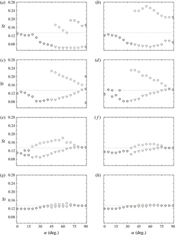
, as is the flow structure (figure 2). Figure 4 presents the dependence of
 $St$
, measured in both upstream- and downstream-cylinder wakes, on
 ${\it\alpha}$
for
 $P^{\ast }=1.5{-}5.0$
, where
 $St_{0}$
is also given as a reference. We may roughly divide this dependence into three different groups for discussion. At
 $P^{\ast }=1.5$
,
 $St$
exhibits a sudden jump in both narrow and wide streets (figure 4
a), apparently distinct from others. The separated shear layer may or may not reattach on the downstream cylinder over
 $P^{\ast }=2.0{-}3.5$
, producing a sudden jump in
 $St$
in the upstream-cylinder wake (figure 4
b–e). This reattachment does not occur for
 $P^{\ast }>3.5$
(figure 4
e–h).
Variation in
 $St$
with
 ${\it\alpha}$
: (a)
 $P^{\ast }=1.5$
, (b) 2.0, (c) 2.5, (d) 3.0, (e) 3.5, (f) 4.0, (g) 4.5 and (h) 5.0 (○, upstream cylinder; ▿, downstream cylinder;
 $\cdots \cdots$
, single cylinder). Measurements were made at
 $(x^{\ast },y^{\ast })=(4,-4)$
and (4, 4).
 $Re=1.3\times 10^{4}$
.

At
 $P^{\ast }=1.5$
, a single
 $St$
, identical in both upstream- and downstream-cylinder wakes, occurs at
 ${\it\alpha}\leqslant 45^{\circ }$
. The two cylinders behave like a single structure, though the effective width of the two cylinders plays a role, causing a smaller
 $St$
than
 $St_{0}$
. At
 ${\it\alpha}<15^{\circ }$
,
 $St$
decreases slowly with an increase in
 ${\it\alpha}$
. Accordingly, the lower shear layer from the upstream cylinder rolls up behind the downstream cylinder without reattachment and the upper shear layer reattaches on the upper surface of the downstream cylinder (figure 2
a), its reattachment point shifting toward the leading corner for higher
 ${\it\alpha}$
. For
 ${\it\alpha}=15^{\circ }{-}20^{\circ }$
, the upper shear layer reattaches on the surfaces around the upper leading corner (figure 2
b), resulting in an enhanced mixing in the shear layer and hence an appreciable recovery in
 $St$
(figure 4
a). As
 ${\it\alpha}$
increases further from
 $20^{\circ }$
to
 $40^{\circ }$
, the shear layer impinges on the front surface of the downstream cylinder (figure 2
c), its impingement position moving away from the upper leading corner to the nominal stagnation point from
 ${\it\alpha}=20^{\circ }$
to
 $35^{\circ }$
and then to the lower leading corner from
 ${\it\alpha}=35^{\circ }$
to
 $40^{\circ }$
. Accordingly, the flow is retarded and modified to a great degree by the downstream cylinder, taking a longer time to complete one vortex shedding cycle and hence producing a rather rapid drop in
 $St$
from
 ${\it\alpha}=20^{\circ }$
to
 $35^{\circ }$
and a less rapid drop from
 ${\it\alpha}=35^{\circ }$
to
 $40^{\circ }$
. Note that a larger
 ${\it\alpha}$
corresponds to a larger effective body width, which also contributes to the decreasing
 $St$
from
 ${\it\alpha}=20^{\circ }$
to
 $40^{\circ }$
. At
 ${\it\alpha}=45^{\circ }$
, the shear layer fails to impinge upon the downstream cylinder and flows through the gap (figure 2
d). Once
 $45^{\circ }<{\it\alpha}\leqslant 65^{\circ }$
, the gap flow gains adequate strength to divide the wake into narrow and wide streets behind the upstream and downstream cylinders, respectively (figure 2
e), associated with the higher and lower
 $St$
, respectively (figure 4
a). Since a larger
 ${\it\alpha}$
allows the gap flow to be less biased or allows a growth in the narrow street width, the higher
 $St$
drops almost linearly, reaching
 $St_{0}=0.134$
at
 ${\it\alpha}=65^{\circ }$
. Interestingly, the high and low
 $St$
correspond to the upstream and downstream cylinders, respectively, for
 ${\it\alpha}=45^{\circ }{-}65^{\circ }$
but swap their correspondence to the cylinders for
 ${\it\alpha}>65^{\circ }$
(figure 4
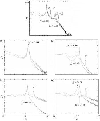
a). The power spectral density functions
 $E_{u}$
of
 $u$
measured on the free-stream sides of the two cylinders, i.e. at
 $(x^{\ast },y^{\ast })=(4,-4)$
and (4, 4), respectively (figure 5
a), indeed show that the higher
 $St$
, i.e.
 $f_{2}^{\ast }$
, dominates in the street behind the upstream cylinder at
 ${\it\alpha}=55^{\circ }$
. The peak at the lower
 $St$
, i.e.
 $f_{1}^{\ast }$
, is comparable in strength on both sides, as observed by Hu & Zhou (Reference Hu and Zhou2008). The higher
 $St$
is almost three times the lower at
 ${\it\alpha}=90^{\circ }$
. The gap flow may be now biased to either side, that is, the vortex street behind either cylinder can be associated with the lower or higher
 $St$
, as presented in figure 4(a).
Typical power spectra,
 $E_{u}$
, of the streamwise fluctuating velocity
 $u$
measured at
 $(x^{\ast },y^{\ast })=(4,-4)$
and (4, 4) for (a)
 $P^{\ast }=1.5$
,
 ${\it\alpha}=55^{\circ }$
, (b) 3.0,
 $5^{\circ }$
, (c) 3.0,
 $10^{\circ }$
, (d) 4.0,
 $25^{\circ }$
, (e) 4.0,
 $35^{\circ }$
,
 $Re=1.3\times 10^{4}$
. The dashed and solid curves denote upstream and downstream cylinders, respectively.

Consider the case of
 $P^{\ast }=2.0{-}3.5$
. Given
 ${\it\alpha}<35^{\circ }{-}40^{\circ }$
, the two cylinders behave like a single bluff body, generating a single Kármán street and hence a single
 $St$
(figure 4
b–e). The
 $St$
rises slightly up to
 ${\it\alpha}=5^{\circ }$
and then decreases. As at
 $P^{\ast }=1.5$
and
 ${\it\alpha}=15^{\circ }{-}45^{\circ }$
(figure 4
a), the rise is due to the movement of shear layer reattachment position, which reaches the leading corner of the downstream cylinder at
 ${\it\alpha}=5^{\circ }$
(e.g. figure 2
g); the decrease in
 $St$
is linked to the impingement position shifting from the upper to the lower corner, along with an increased effective bluff width for larger
 ${\it\alpha}$
(Alam & Meyer Reference Alam and Meyer2013). The shear layer goes through the gap, without reattachment, at
 ${\it\alpha}>30^{\circ }$
,
 $25^{\circ }$
and
 $20^{\circ }$
for
 $P^{\ast }=2.0$
, 2.5 and 3.0, respectively. The gap flow, deflected toward the upstream cylinder, is weak and does not play a significant role in the dynamics over
 ${\it\alpha}=30^{\circ }{-}35^{\circ }$
at
 $P^{\ast }=2.0$
,
 $25^{\circ }{-}40^{\circ }$
at
 $P^{\ast }=2.5$
and
 $20^{\circ }{-}30^{\circ }$
at
 $P^{\ast }=3.0$
. For a higher
 ${\it\alpha}$
, the gap flow acts as a base bleed and prolongs the formation length (e.g. Zhou et al.
Reference Zhou, Wang, So, Xu and Jin2001; Alam & Meyer Reference Alam and Meyer2011), thus increasing
 $St$
(Alam et al.
Reference Alam, Moriya and Sakamoto2003a
, Reference Alam, Zhou and Wang2011), but the increased effective bluff width reduces
 $St$
(Alam & Sakamoto Reference Alam and Sakamoto2005). The two effects tend to cancel each other and
 $St$
varies little. A further increase in
 ${\it\alpha}$
allows the deflected gap flow to grow in strength, and a narrow and a wide street emerge, corresponding to a higher and lower
 $St$
, respectively (figure 4
b–d). As
 ${\it\alpha}$
approaches
 $90^{\circ }$
, the gap flow appears symmetric about
 $y^{\ast }=0$
, forming two coupled vortex streets (e.g. figure 2
k), except at
 $P^{\ast }=2.0$
where the narrow and wide streets persist and the gap flow may be deflected to either side.
Note the occurrence of two
 $St$
at
 ${\it\alpha}=10^{\circ }$
and
 $20^{\circ }$
at
 $P^{\ast }=3.0$
. The downstream cylinder is subjected to the impingement of the shear layer (figure 2
g), which is unsteady for a relatively large
 $P^{\ast }$
. The flow physics behind the observation may be understood through examining
 $E_{u}$
, along with flow visualization data (figure 2). At
 ${\it\alpha}=5^{\circ }$
the shear layer reattaches very near the upper leading corner of the downstream cylinder (figure 2
g) and
 $E_{u}$
displays one pronounced peak at
 $f^{\ast }=0.138$
(figure 5
b). At
 ${\it\alpha}=10^{\circ }$
(figure 5
c), the pronounced peak occurs at
 $f_{2}^{\ast }=0.134$
accompanied by another peak at
 $f_{1}^{\ast }=0.104$
behind both cylinders. Evidently, this shear layer impingement occurs intermittently on the upper leading corner and front surface of the downstream cylinder, and the bi-stable nature of the flow is responsible for
 $f_{1}^{\ast }$
and
 $f_{2}^{\ast }$
. However, the shear layer impinges only upon the front surface as
 ${\it\alpha}$
increases to
 $15^{\circ }$
(figure 2
h). This is followed by the resumption of a single
 $St=0.111$
(figure 4
d), which is almost equal to
 $f_{1}^{\ast }\,(=0.104)$
at
 ${\it\alpha}=10^{\circ }$
(figure 5
c). This is not coincidental; both frequencies are connected to the shear layer impingement upon the front surface of the downstream cylinder. Interestingly, the second harmonic of
 $St$
was absent at
 ${\it\alpha}=5^{\circ }$
but evident behind the upstream cylinder at
 ${\it\alpha}=15^{\circ }$
. The difference arises from the reattachment/impingement location, i.e. one
 $({\it\alpha}=5^{\circ })$
on the leading corner of the downstream cylinder and the other
 $({\it\alpha}=15^{\circ })$
upon the front surface. The latter is associated with the second harmonic peak in
 $E_{u}$
. Alam et al. (Reference Alam, Moriya, Takai and Sakamoto2003b
) and Alam (Reference Alam2014) observed, in the wake of two tandem circular cylinders at
 $P^{\ast }=1.4$
, the second harmonic frequency in the power spectrum of the fluctuating pressure on the cylinder surface when the shear layers from the upstream cylinder impinged upon the downstream cylinder, forming a strong quasi-steady vortex between the cylinders. The second harmonic frequency disappeared at
 $P^{\ast }=3.5$
where the shear layer impingement was greatly weakened. By
 ${\it\alpha}=20^{\circ }$
, the shear layer either impinges upon the lower leading corner or passes through the gap without reattachment (figure 2
i) and is again bi-stable.
 $E_{u}$
at
 ${\it\alpha}=20^{\circ }$
(not shown) was quite similar to its counterpart at
 ${\it\alpha}=10^{\circ }$
in figure 5(c), showing two significant peaks at
 $f_{1}^{\ast }$
and
 $f_{2}^{\ast }$
and another peak at
 $2f_{2}^{\ast }$
only behind the upstream cylinder. There are differences between the two cases though. Firstly, while reattaching/impinging intermittently on the upper leading corner and front surface of the downstream cylinder at
 ${\it\alpha}=10^{\circ }$
, the unsteady shear layer intermittently impinges upon the front surface near the lower leading corner and flows through the gap, without reattachment, at
 ${\it\alpha}=20^{\circ }$
. Secondly, the higher and lower
 $St$
are associated with the shear layer reattachment on the upper leading corner and front surface, respectively, at
 ${\it\alpha}=10^{\circ }$
but are connected to reattachment on the lower corner and the non-reattached flow, respectively, at
 ${\it\alpha}=20^{\circ }$
.
At
 $P^{\ast }=3.5$
(figure 4
e), the shear layer impinges upon the front surface for
 ${\it\alpha}\leqslant 5^{\circ }$
and a single
 $St$
is observed. At
 ${\it\alpha}=10^{\circ }$
and
 $15^{\circ }$
, two different
 $St$
are observed, due to intermittent shear layer reattachment and non-reattachment. At
 ${\it\alpha}\geqslant 20^{\circ }$
, both inner shear layers go through the gap, splitting the wake into one narrow and one wide street behind the upstream and downstream cylinders, respectively. Gaining a large momentum under large
 $P^{\ast }$
, the gap flow is less deflected (Wang & Zhou Reference Wang and Zhou2005; Alam & Zhou Reference Alam and Zhou2013), implying a rather limited departure in width between the two streets and hence a small difference between the high and low
 $St$
. For larger
 ${\it\alpha}$
, beyond
 $20^{\circ }$
, the lateral and longitudinal separations between the cylinders increase and decrease, respectively. The former tends to reduce the difference between the two
 $St$
, while the latter acts to enlarge it, narrowing the street behind the upstream cylinder. The two effects tend to cancel out each other, maintaining the difference almost unchanged up to
 ${\it\alpha}=60^{\circ }$
. At
 ${\it\alpha}>60^{\circ }$
, the latter effect retreats gradually, leading to a collapse of the two
 $St$
to
 $St_{0}$
at
 ${\it\alpha}\geqslant 80^{\circ }$
.
For
 $P^{\ast }\geqslant 4.0$
, the shear layers roll up, forming vortices, before reaching the downstream cylinder. At
 ${\it\alpha}=0^{\circ }$
, vortex shedding from the downstream cylinder is triggered by the arrival of vortices from the upstream cylinder, implying the same
 $St$
in the gap as that behind the cylinders. At
 ${\it\alpha}>0^{\circ }$
, the upper-row vortices from the upstream cylinder impinge on the front (e.g. figure 2
l) or lower surface (e.g. figure 2
m) of the downstream cylinder, depending on
 ${\it\alpha}$
. Their direct interaction with shear layers around the downstream cylinder results in synchronized shedding from the two cylinders and a single
 $St$
, which prevails up to
 ${\it\alpha}=30^{\circ }$
,
 $35^{\circ }$
and
 $40^{\circ }$
for
 $P^{\ast }=4.0$
, 4.5 and 5.0, respectively (figure 4
f–h). Typical
 $E_{u}$
is presented in figure 5(d). The
 ${\it\alpha}$
range of the single
 $St$
is enlarged at larger
 $P^{\ast }$
because the two rows of vortices from the upstream cylinder grow laterally downstream. The
 $St$
is weakly dependent on
 $P^{\ast }$
and is nearly constant up to at least
 ${\it\alpha}=15^{\circ }$
, linked to the vortex impingement on the front surface, before a slow rise with
 ${\it\alpha}$
when the vortices hit the lower surface of the cylinder. At
 ${\it\alpha}=30^{\circ }{-}75^{\circ }$
,
 $35^{\circ }{-}70^{\circ }$
and
 $0^{\circ }{-}70^{\circ }$
for
 $P^{\ast }=4.0$
, 4.5 and 5.0, respectively, the upstream-cylinder-generated vortex street cannot trigger vortex shedding from the downstream cylinder anymore, and is narrowed under the squeezing effect of the downstream cylinder, resulting in a higher
 $St$
, as illustrated in figure 5(e). The difference in
 $St$
between the two streets contracts for higher
 $P^{\ast }$
where the street behind the upstream cylinder is less squeezed. A further increase in
 ${\it\alpha}$
leads to negligibly small interference between the streets, their
 $St$
values collapsing to
 $St_{0}$
.
4.3 Dependence of
 $St$
on
$P^{\ast }$
and
${\it\alpha}$


The overall picture of
 $St$
may be obtained via examining the dependence of
 $St$
on
 $P^{\ast }$
and
 ${\it\alpha}$
. Under very complicated and complex interactions between the shear layers, between shear layers and vortices and between vortices, the flow structure may evolve downstream very rapidly, particularly in the near wake. Naturally, the measured
 $St$
may vary with
 $x^{\ast }$
as well as from one street to another. It has been found that
 $St$
obtained at
 $x^{\ast }=4$
can be different from that at
 $x^{\ast }=7$
, 10 and 15, though
 $St$
remains unchanged for
 $x^{\ast }\geqslant 7$
. As such, the data measured at
 $x^{\ast }=4$
and 10 are presented and discussed below.
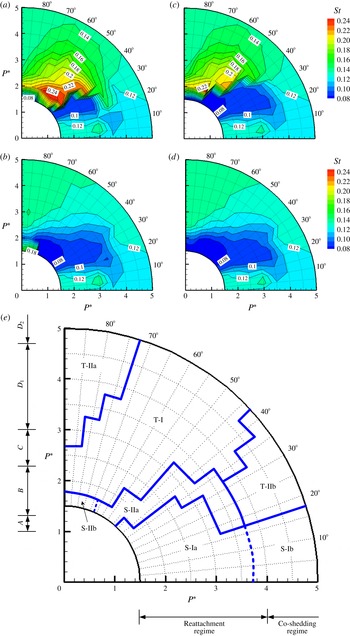
At
 $x^{\ast }=4$
,
 $St$
behind the upstream cylinder is 0.10–0.13 at
 ${\it\alpha}<20^{\circ }$
(figure 6
a), less than
 $St_{0}\,(=0.134)$
. This is because the downstream cylinder obstructs the wake of the upstream cylinder when
 $P^{\ast }\geqslant 4$
or directly interacts with the shear layer around the upstream cylinder when
 $P^{\ast }<4$
, widening the combined wake.
 $St$
is thus identical to that behind the downstream cylinder (figure 6
b). At
 $P^{\ast }<4$
, the outer shear layers of the two cylinders roll up, forming vortices at the same
 $St$
, and the cylinders behave like a single bluff body. On the other hand, at
 $P^{\ast }\geqslant 4$
a single
 $St$
is achieved due to vortex shedding from the downstream cylinder triggered by the arrival of the upstream-cylinder-generated vortices.
Isocontours of
 $St$
: (a)
 $x^{\ast }=4$
, upstream cylinder; (b) 4, downstream; (c) 10, upstream; (d) 10, downstream. The
 $\text{contour increment}=0.01$
.
 $Re=1.3\times 10^{4}$
. (e) Dependence of the flow regime on
 $P^{\ast }$
and
 ${\it\alpha}\,(Re=1.3\times 10^{4})$
. Alam et al.’s (Reference Alam, Zhou and Wang2011,
 $Re=4.7\times 10^{4}$
) data (
 $A$
,
 $B$
,
 $C$
,
 $D_{1}$
,
 $D_{2}$
) for the side-by-side arrangement and Sakamoto et al.’s (Reference Sakamoto, Haniu and Obata1987,
 $Re=2.76\times 10^{4}$
) data (reattachment and co-shedding regimes) for the tandem cylinders are also included.
 $A$
: single-body regime,
 $B$
: two-frequency regime,
 $C$
: transition regime,
 $D_{1}$
: antiphase-dominated two-street regime,
 $D_{2}$
: antiphase-inphase-mixed two-street regime.

For
 $1.5<P^{\ast }<3.0$
,
 $St$
drops to 0.07–0.08 and is identical from one street to another given
 ${\it\alpha}=25^{\circ }{-}40^{\circ }$
(figure 6
a,b). With a weak gap flow, vortex shedding from the free-stream sides of the two cylinders dominates the wake, leading to a single
 $St$
, which varies little with
 ${\it\alpha}$
and
 $P^{\ast }$
. With a further increase in
 ${\it\alpha}$
or
 $P^{\ast }$
, the formation of a narrow and a wide street leads to a higher
 $St$
behind the upstream cylinder (figure 6
a) than behind the downstream (figure 6
b). The former drops rapidly for larger
 ${\it\alpha}$
or
 $P^{\ast }$
, while the latter goes up, both reaching
 $St_{0}$
for
 ${\it\alpha}>70^{\circ }{-}85^{\circ }$
or
 $P^{\ast }>2.5$
. The highest
 $St\,({\approx}0.25)$
or
 $St/St_{0}\,(=1.87)$
associated with the upstream cylinder occurs at
 $P^{\ast }=2.0$
and
 ${\it\alpha}=55^{\circ }$
. So does the lowest
 $St\,({\approx}\,0.07)$
or
 $St/St_{0}\,(=0.54)$
in the wake of the downstream cylinder. This means that the downstream cylinder at this configuration can squeeze the upstream-cylinder wake most effectively, producing the largest difference in
 $St$
between the two streets. In the wake of two circular cylinders, Kiya et al. (Reference Kiya, Arie, Tamura and Mori1980,
 $Re=1.58\times 10^{4}$
) observed the highest
 $St=0.39$
or
 $St/St_{0}=1.95$
and lowest
 $St=0.11$
or
 $St/St_{0}=0.55$
behind the upstream and downstream cylinders, respectively, at
 ${\it\alpha}=35^{\circ }{-}45^{\circ }$
and
 $P^{\ast }\approx 1.8$
. The highest or lowest
 $St/St_{0}$
and corresponding
 $P^{\ast }$
are quite close for the two cases, though
 ${\it\alpha}$
is larger in the case of square cylinders. This is not unexpected in view of the fact that both flow separation angle and wake width are larger in the wake of square cylinders than in the wake of circular cylinders. A further increase in
 ${\it\alpha}$
or
 $P^{\ast }$
leads to a diminishing difference in
 $St$
between the streets until
 $St=St_{0}$
.
At
 $P^{\ast }\leqslant 1.5$
and
 ${\it\alpha}>70^{\circ }$
, the higher and lower
 $St$
correspond now to the downstream and upstream cylinders, respectively. As
 ${\it\alpha}$
increases, the higher
 $St$
drops, while the other remains almost unchanged.
At
 $x^{\ast }=10$
(figure 6
c,d), the dependence of
 $St$
on
 ${\it\alpha}$
and
 $P^{\ast }$
is overall similar to that at
 $x^{\ast }=4$
(figure 6
a,b). However, there are two differences. Firstly, the higher
 $St$
behind the upstream cylinder at
 $35^{\circ }<{\it\alpha}<65^{\circ }$
for
 $1.5<P^{\ast }<3.0$
and
 $20^{\circ }<{\it\alpha}<35^{\circ }$
for
 $3<P^{\ast }<4$
(figure 6
a) decreases at
 $x^{\ast }=10$
(figure 6
c). Secondly, the higher
 $St$
that occurs at
 ${\it\alpha}>70^{\circ }$
and
 $P^{\ast }\leqslant 1.5$
behind the downstream cylinder at
 $x^{\ast }=4$
(figure 6
b) transmutes to the lower at
 $x^{\ast }=10$
(figure 6
d),
 $St$
becoming identical in both streets. The observation suggests that the vortices of the higher
 $St$
in the narrow street, observed at
 $x^{\ast }\leqslant 4$
, vanish rapidly and are broken up or amalgamated with the vortices of the lower
 $St$
.
5 Flow classification
Flow classification is carried out based on rather exhaustive measurements, including the
 $St$
data extracted from
 $E_{u}$
of
 $u$
measured for a total of 152 geometric configurations at four downstream stations (
 $x^{\ast }=4$
, 7, 10 and 15) and eleven cross-stream positions (
 $y^{\ast }=0$
,
 $\pm 1$
,
 $\pm 2$
,
 $\pm 3$
,
 $\pm 4$
and
 $\pm 5$
) for each
 $x^{\ast }$
. Four distinct flow structures are identified, including two one-street modes (S-I and S-II) and two twin-street modes (T-I and T-II). Modes S-I, S-II and T-II are further divided into two submodes each. Their corresponding regions in the
 $(P^{\ast },{\it\alpha})$
plane are shown in figure 6(e). The thick solid and thick dashed lines divide different flow modes determined from flow visualization and
 $E_{u}$
or
 $St$
at
 $x^{\ast }=4$
–15
 $(Re=1.3\times 10^{4})$
. Flow classifications by Sakamoto et al. (Reference Sakamoto, Haniu and Obata1987) for
 ${\it\alpha}=0^{\circ }$
and Alam et al. (Reference Alam, Zhou and Wang2011) for
 ${\it\alpha}=90^{\circ }$
are also included. The border between different flow modes is identified with the midpoint between two adjacent measurement grid points where the flow structure changes from one mode to another. For example, T-IIb and S-Ib modes are identified at
 ${\it\alpha}=20^{\circ }\,(P^{\ast }\geqslant 4.0)$
and
 ${\it\alpha}=15^{\circ }\,(P^{\ast }\geqslant 4.0)$
, respectively, and the border is then determined at
 ${\it\alpha}=17.5^{\circ }$
(figure 6
e); by the same token, if S-Ia and S-Ib modes are detected at
 $P^{\ast }\leqslant 3.5$
and
 ${\geqslant}4.0\,({\it\alpha}\leqslant 15^{\circ })$
, respectively, the border is at
 $P^{\ast }=3.75$
. Thus, the uncertainty in determining the flow mode is 0.25 and
 $2.5^{\circ }$
for
 $P^{\ast }$
and
 ${\it\alpha}$
, respectively. The typical flow structure in each mode is discussed in detail below.
5.1 Mode S-I
Mode S-I is characterized by a single staggered vortex street with a single
 $St\,(=0.07{-}0.13)$
and is found at
 ${\it\alpha}<47.5^{\circ }{-}17.5^{\circ }$
depending on
 $P^{\ast }$
(figure 6). However, there are two types of vortex formation processes, resulting in very different vortex strengths. Thus, this mode is further divided into S-Ia and S-Ib.
Given
 $P^{\ast }<3.75$
and
 ${\it\alpha}=0^{\circ }{-}47.5^{\circ }$
, the two cylinders behave like one single body. The inner shear layer separated from the upstream cylinder reattaches on the downstream cylinder at smaller
 ${\it\alpha}$
or
 $P^{\ast }$
but goes through the gap at larger
 ${\it\alpha}$
or
 $P^{\ast }$
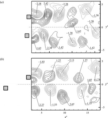
. The outer shear layers separate alternately from the free-stream sides of the cylinders, forming one staggered vortex street or Mode S-Ia. Figure 7(a) presents typical flow structures of PIV-captured instantaneous vorticity contours for mode S-Ia. The maximum vorticity is slightly lower than in a single square cylinder wake (e.g. Lyn et al.
Reference Lyn, Einav, Rodi and Park1995; Hu et al.
Reference Hu, Zhou and Dalton2006), but the vortex wavelength is longer because of the lower
 $St$
(figure 6). Note that both positive and negative vortices grow in strength downstream, at least up to
 $x^{\ast }=15$
. This is a quite typical snapshot. The observation is connected to the way the vortices are generated. Zhou & Yiu (Reference Zhou and Yiu2006) also noted in the wake of two tandem circular cylinders
 $(L^{\ast }=2.5)$
that the shear layer separated from the upstream cylinder reattached on the downstream side of the downstream cylinder, interrupting the development of the boundary layer and impairing the initial vortex strength. As a result, vortices grew in strength under the effect of mean shear all the way until at least
 $x^{\ast }=10$
.
Typical instantaneous PIV-measured vorticity
 ${\it\omega}_{z}^{\ast }$
contours: (a) S-Ia,
 $P^{\ast }=2.5$
,
 ${\it\alpha}=15^{\circ }$
and (b) S-Ib, 4.5,
 $5^{\circ }$
.
 $Re=1.3\times 10^{4}$
. The contour cutoff levels are
 $\pm 0.3$
and the increment is 0.2.

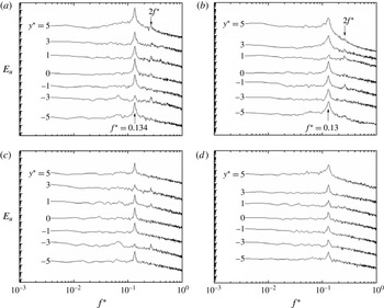
The
 $E_{u}$
for mode S-Ia displays a pronounced peak at
 $f^{\ast }=0.111$
(figure 8
a) at
 $y^{\ast }=0$
,
 $\pm 1$
,
 $\pm 3$
and
 $\pm 5$
. The predominant frequency does not change over
 $x^{\ast }=4{-}10$
. Furthermore, the characteristics of the power spectrum at
 $y^{\ast }>0$
are similar to those at
 $y^{\ast }<0$
, implying a single wake with two rows of vortices at
 $y^{\ast }>0$
and
 $y^{\ast }<0$
, respectively, consistent with PIV data (figure 7
a). Peaks at the second and even third harmonics of
 $St$
are discernible in
 $E_{u}$
up to
 $x^{\ast }=10$
(figure 8
c), especially near the wake centreline.
Typical
 $E_{u}$
of
 $u$
measured at (a,b)
 $x^{\ast }=4$
and (c,d)
 $x^{\ast }=10$
for mode S-Ia (a,c,
 $P^{\ast }=2.5$
,
 ${\it\alpha}=15^{\circ }$
) and mode S-Ib (b,d,
 $P^{\ast }=4.5$
,
 ${\it\alpha}=5^{\circ }$
).
 $Re=1.3\times 10^{4}$
.

Mode S-Ib occurs at
 $P^{\ast }>3.75$
and
 ${\it\alpha}<17.5^{\circ }$
(figure 6
e), featuring vortex shedding from both cylinders at the same
 $St$
(figure 6). At
 ${\it\alpha}=0^{\circ }$
, mode S-Ib corresponds to the co-shedding flow (e.g. Sakamoto & Haniu Reference Sakamoto and Haniu1988b
; Ljungkrona, Norberg & Sunden Reference Ljungkrona, Norberg and Sunden1991; Alam et al.
Reference Alam, Moriya, Takai and Sakamoto2002; Zhou & Yiu Reference Zhou and Yiu2006), and its
 ${\it\omega}_{z}^{\ast }$
-contours at
 $P^{\ast }=4.5$
and
 ${\it\alpha}=5^{\circ }$
are presented in figure 7(b). Similarly to mode S-Ia (figure 7
a), a staggered vortex street about the centreline is evident in mode S-Ib. However, the initial conditions of modes S-Ia and S-Ib are different. Mode S-Ia is characterized by a smaller
 $P^{\ast }$
. With the inner shear layer from the upstream cylinder reattaching on the downstream cylinder, the staggered vortices originate largely from alternate shedding from the free-stream sides of the cylinders. On the other hand, S-Ib is characterized by vortex impingement on the downstream cylinder and the staggered vortices behind the cylinders result from interactions between the upstream-cylinder-generated vortices and the upper or lower shear layer, depending on
 $P^{\ast }$
and
 ${\it\alpha}$
(figure 6
a–d), around the downstream cylinder. This impingement reduces substantially the vortex strength. For instance, the vortices in figure 7(b) are significantly smaller in both maximum vorticity and size than those in figure 7(a). Hu & Zhou (Reference Hu and Zhou2008) made a similar finding in the wake of two staggered circular cylinders. Furthermore, the upper-row vortices appear weaker than the lower (figure 7
b), as a result of interactions between impinging vortices and the upper shear layer. The PIV results are supported by
 $E_{u}$
(figure 8
b,d) measured at the same
 $P^{\ast }$
and
 ${\it\alpha}$
, which show a pronounced peak at
 $f^{\ast }=0.119$
in
 $E_{u}$
, indicating the occurrence of predominant vortices. However, this peak is considerably weaker than that in figure 8(a,c). This peak also decays more rapidly with increasing
 $x^{\ast }$
for S-Ib than for S-Ia. On another note, this peak is quite evident near the wake centreline for S-Ia but not so for S-Ib. This is because S-Ib consists of weaker and smaller vortices and a larger lateral separation between the two rows of vortices, which is obvious by comparing figure 7(a) with (b).
Note that S-Ia and S-Ib are separated by
 $P^{\ast }=3.75$
at
 ${\it\alpha}=0^{\circ }$
(figure 6
e), which is consistent with previous classifications for the wake of two tandem cylinders. Based on the measured force and
 $St$
at
 $Re=2.76{-}5.52\times 10^{4}\,({\it\alpha}=0^{\circ })$
, Sakamoto et al. (Reference Sakamoto, Haniu and Obata1987) and Sakamoto & Haniu (Reference Sakamoto and Haniu1988a
) reported
 $P_{cri}^{\ast }=4.0$
. The
 $P_{cri}^{\ast }$
was found to be 3.5–3.75 by Luo & Teng (Reference Luo and Teng1990) based on force measurement at
 $Re=5.67\times 10^{4}$
. It is worthwhile pointing out that the
 $P_{cri}^{\ast }$
is highly dependent on the free-stream turbulent intensity (Sakamoto & Haniu Reference Sakamoto and Haniu1988a
) and
 $Re$
as well as how
 $P^{\ast }$
is varied, i.e. progressively increasing or decreasing (Liu & Chen Reference Liu and Chen2002).
5.2 Mode S-II
Mode S-II occurs in general at large
 ${\it\alpha}\,({>}17.5^{\circ })$
and small
 $P^{\ast }\,({<}3.75)$
; the larger the
 ${\it\alpha}$
, the smaller the
 $P^{\ast }$
as long as the lateral separation between the cylinders is adequate for the formation of two counter-rotating vortices in the gap (figure 2
e). Now each cylinder generates one Kármán vortex street, one narrow with a higher
 $St$
and the other wide with a lower
 $St$
. Vigorous interactions take place between the two streets, resulting in one single vortex street of the low
 $St$
at
 $x^{\ast }>7$
(depending on
 $Re$
). The narrow street may occur behind the upstream or downstream cylinder (figure 2
e,f), referred to as S-IIa and S-IIb, respectively.
S-IIa occupies a much larger region than S-IIb (figure 6
e). In this region, the upstream cylinder generates vortices at a higher
 $St$
at
 $x^{\ast }<7$
(figure 6
a), but these vortices evolve into a lower
 $St$
at
 $x^{\ast }>7$
(figure 6
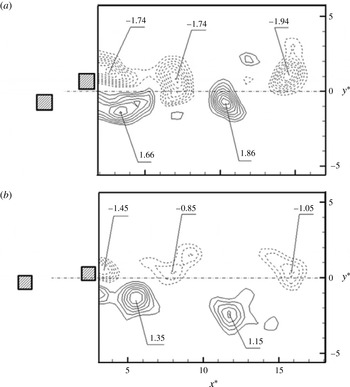
c). Based on the PIV data (figure 9
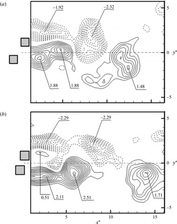
a), it is seen that the gap flow is dominated by positive vorticity (induced mainly by the lower side of the downstream cylinder) which can also be predicted from figure 2(e). One may recognize that the merging of two positive-signed vortices, one from the lower side of the upstream cylinder (maximum
 ${\it\omega}_{z}^{\ast }=1.88$
, lower one) and the other (maximum
 ${\it\omega}_{z}^{\ast }=1.88$
, upper one) from the gap, enlarges the size of the resultant vortex in the lower street, whose maximum
 ${\it\omega}_{z}^{\ast }$
drops to 1.48 at
 $x^{\ast }\approx 12$
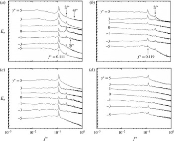
. Typical
 $E_{u}$
of
 $u$
at
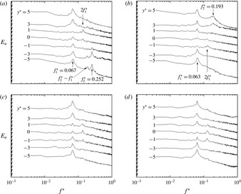
 $x^{\ast }=4$
and 10 for mode S-IIa are presented in figure 10(a,c) for a representative configuration of
 $P^{\ast }=2.0$
and
 ${\it\alpha}=60^{\circ }$
. At
 $y^{\ast }>0$
, only the peak at
 $f_{1}^{\ast }=0.067$
and/or its second harmonic is evident at either
 $x^{\ast }$
, suggesting the occurrence of the predominant vortices in the wide street behind the downstream cylinder. On the other hand, a peak at
 $f_{2}^{\ast }=0.252$
appears at
 $y^{\ast }<0$
for
 $x^{\ast }=4$
(figure 10
a) due to the presence of a downward-deflected narrow street behind the upstream cylinder. Interestingly, a minor peak occurs at
 $f_{2}^{\ast }$
–
 $f_{1}^{\ast }$
only for
 $y^{\ast }<0$
at
 $x^{\ast }=4$
, reflecting vigorous interactions in the narrow street. The peak at
 $f_{1}^{\ast }$
is more pronounced at
 $y^{\ast }>0$
than at
 $y^{\ast }<0$
, corroborating the observation from figure 9(a).
Typical instantaneous PIV-measured vorticity
 ${\it\omega}_{z}^{\ast }$
contours: (a) S-IIa,
 $P^{\ast }=2.0$
,
 ${\it\alpha}=60^{\circ }$
and (b) S-IIb, 1.5,
 $80^{\circ }$
.
 $Re=1.3\times 10^{4}$
. The contour cutoff levels are
 $\pm 0.3$
and the increment is 0.2.

Typical
 $E_{u}$
of
 $u$
measured at (a,b)
 $x^{\ast }=4$
and (c,d)
 $x^{\ast }=10$
for mode S-IIa (a,c,
 $P^{\ast }=2.0$
,
 ${\it\alpha}=60^{\circ }$
) and mode S-IIb (b,d,
 $P^{\ast }=1.5$
,
 ${\it\alpha}=80^{\circ }$
).
 $Re=1.3\times 10^{4}$
.

Mode S-IIb takes place at
 ${\it\alpha}>67.5^{\circ }$
and
 $P^{\ast }<1.75$
. In contrast to S-IIa, this mode is characterized by a gap flow deflected toward the downstream cylinder, forming a narrow and a wide street behind the downstream and upstream cylinders, respectively. The flow structure corresponding to mode S-IIb has been presented and discussed earlier (figure 2
f). Figure 9(b) presents the PIV-measured
 ${\it\omega}_{z}^{\ast }$
-contours at
 $P^{\ast }=1.5$
and
 ${\it\alpha}=80^{\circ }$
. The vorticity concentrations associated with the gap flow are discernible, echoing the change in the gap flow direction from the lower to the upper (figure 2
f). The presence of the positive vorticity, with a maximum of 0.51, behind the downstream cylinder bears the signature of the gap flow being biased upward. Typical
 $E_{u}$
(figure 10
b,d) at
 $P^{\ast }=1.5$
and
 ${\it\alpha}=80^{\circ }$
exhibits a pronounced peak at
 $f_{1}^{\ast }=0.063$
across the wake at
 $x^{\ast }=4$
and 10 and another broad peak at
 $f_{2}^{\ast }=0.193$
only at
 $x^{\ast }=4$
and
 $y^{\ast }>0$
(figure 10
b). Apparently, the peak at
 $f_{1}^{\ast }$
is more pronounced at
 $y^{\ast }<0$
than at
 $y^{\ast }>0$
. The observations are consistent with the flow visualization data (figure 2
f).
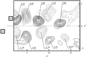
Typical instantaneous PIV-measured vorticity
 ${\it\omega}_{z}^{\ast }$
contours at
 $P^{\ast }=4.0$
,
 ${\it\alpha}=55^{\circ }$
; mode T-I.
 $Re=1.3\times 10^{4}$
.

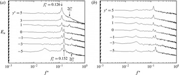
Typical
 $E_{u}$
of
 $u$
measured at (a)
 $x^{\ast }=4$
and (b)
 $x^{\ast }=10$
for mode T-I (
 $P^{\ast }=4.0$
,
 ${\it\alpha}=55^{\circ }$
).
 $Re=1.3\times 10^{4}$
.

5.3 Mode T-I
Mode T-I occurs at a larger
 $P^{\ast }$
or
 ${\it\alpha}\,(P^{\ast }>1.75,32.5^{\circ }<{\it\alpha}<90^{\circ })$
than S-II. A large
 $P^{\ast }$
or
 ${\it\alpha}$
implies a large momentum of the gap flow and also a large separation between the two counter-rotating gap vortices. Consequently, the narrow and wide streets do not merge downstream and, instead, retain their identities with high and low
 $St$
, respectively. With a variation in
 $P^{\ast }$
or
 ${\it\alpha}$
, the higher
 $St$
behind the upstream cylinder drops from 0.22 to 0.13, but the lower
 $St$
behind the downstream cylinder increases from 0.08 to 0.13 (figure 6). As illustrated in figure 11, the two vortex streets appear to be qualitatively the same. Actually, the upstream-cylinder-generated street is narrower than the downstream-cylinder-generated one. A smaller streamwise separation between the two consecutive vortices in the narrow street compared to that in the wide street suggests a higher
 $St$
. Both streets display staggered vortices, with an appreciably larger size and strength of vortices for the upper street. With a lower frequency, vortex shedding from the downstream cylinder may have more time, than that from the upstream cylinder, to accumulate vorticity (Zdravkovich Reference Zdravkovich1985), yielding the vortices of a larger size and strength and hence a wider street. Naturally, mode T-I is asymmetric about
 $y^{\ast }=0$
. The interactions between the two streets of different
 $St$
however accelerate the downstream decay of vortices (Sumner et al.
Reference Sumner, Price and Paidoussis2000; Zhou, Zhang & Yiu Reference Zhou, Zhang and Yiu2002; Alam & Zhou Reference Alam and Zhou2013). It will be shown later that two antiphased streets of an identical
 $St$
persist longer downstream. The two distinct predominant frequencies in the two streets are confirmed by
 $E_{u}$
(figure 12) at
 $P^{\ast }=4.0$
and
 ${\it\alpha}=55^{\circ }$
. Two pronounced peaks occur at
 $f_{1}^{\ast }=0.126$
and
 $f_{2}^{\ast }=0.152$
above and below the centreline, respectively, in the downstream- and upstream-cylinder-generated streets. The two frequencies are lower and higher than that (0.134) in an isolated square cylinder wake, respectively. Note that both peaks at
 $f_{1}^{\ast }$
and
 $f_{2}^{\ast }$
may occur over
 $y^{\ast }=-1{-}+1$
, that is, both predominant frequencies are detectable in the inner rows of the two streets, in contrast to the observation in S-IIb where the low
 $St$
occurs across the narrow street as well (figure 10). The peaks at
 $f_{1}^{\ast }$
and
 $f_{2}^{\ast }$
decay rather rapidly for larger
 $x^{\ast }$
, as a result from the interactions between the two streets of distinct frequencies as well as the mechanisms associated with an isolated cylinder wake. Landweber (Reference Landweber1942) analysed the stability of two streets based on a model of infinitely long rows of point vortices, similarly to the classical von Kármán analysis of a single vortex street (Zdravkovich Reference Zdravkovich1997). He came to the conclusion that, given two stable streets, the convection velocity must be the same for all vortices and the two streets must be either antiphased or inphased. As such, it may be inferred that if two streets differ in width, their phase shift will change and the flow structure will be unstable, accelerating the decaying rate.
5.4 Mode T-II
The difference in
 $St$
between the narrow and wide streets dwindles as
 $P^{\ast }$
increases (figure 4). For
 $P^{\ast }>2.75$
and
 ${\it\alpha}>72.5^{\circ }$
, this difference is no more than 1 %, comparable to the experimental uncertainty. Apparently, such a flow is different from T-I and is called T-II. Mode T-II occurs in two regions of the
 $P^{\ast }$
–
 ${\it\alpha}$
plane (figure 6
e), i.e. mode T-IIa at large
 ${\it\alpha}\,({>}72.5^{\circ })$
and
 $P^{\ast }>2.75$
and mode T-IIb at
 $17.5^{\circ }\leqslant {\it\alpha}<42.5^{\circ }$
and large
 $P^{\ast }\,({>}3.75)$
. In mode T-II, the predominant frequencies in both streets are identical to each other and almost the same as that (0.134) in an isolated cylinder wake. Vortices shed from the two cylinders are synchronized, either antiphased or inphased. T-IIa and T-IIb are distinguished from each other based on their different synchronization mechanisms and initial conditions.
Mode T-IIa resembles the flow structure behind two side-by-side cylinders (Alam et al.
Reference Alam, Zhou and Wang2011). The two cylinders generate individual streets of the same shedding frequency and a similar width. Typical instantaneous
 ${\it\omega}_{z}^{\ast }$
contours at
 $P^{\ast }=4.5$
and
 ${\it\alpha}=85^{\circ }$
are illustrated in figure 13(a). The wake consists of two Kármán vortex streets of the same width and frequency, which are either antiphased (figure 13
a) or inphased (not shown). The
 ${\it\omega}_{z}^{\ast }$
-contours indicate comparable vortex strengths between the two coupled streets, which are essentially the same as in an isolated square cylinder wake (Hu et al.
Reference Hu, Zhou and Dalton2006). The observations are further supported by
 $E_{u}$
(figure 14
a,c) measured at
 $P^{\ast }=4.5$
and
 ${\it\alpha}=85^{\circ }$
, which shows a pronounced peak at
 $St=0.134$
across the wake at both
 $x^{\ast }=4$
and 10. A comparison in
 $E_{u}$
between figures 12 and 14 indicates that T-IIa is more stable than T-I. The coupling between the streets is largely dictated by vortex shedding associated with the gap flow (Alam et al.
Reference Alam, Moriya and Sakamoto2003a
; Alam & Zhou Reference Alam and Zhou2013) and the antiphased shedding overwhelms the inphased. The inphased vortex shedding occurs occasionally based on the PIV data. Alam et al. (Reference Alam, Zhou and Wang2011) observed in the wake of two side-by-side square cylinders approximately 65 % of antiphased shedding at
 $P^{\ast }=3.0$
. This percentage dropped to 25 % at
 $P^{\ast }=5.0$
. On the other hand, the inphased shedding was 2 % and 14 % at
 $P^{\ast }=3.0$
and 5.0, respectively. Kamemoto (Reference Kamemoto1976,
 $Re=3\times 10^{4}$
) and Alam et al. (Reference Alam, Moriya and Sakamoto2003a
,
 $Re=5.5\times 10^{4}$
) showed in the wake of two side-by-side circular cylinders that vortices shed from the two cylinders were predominantly antiphased at
 $P^{\ast }=2.1{-}3.5$
but both antiphased and inphased at
 $P^{\ast }>3.5$
. Alam & Zhou (Reference Alam and Zhou2013) showed at
 $Re=300$
that the antiphased street persists for a longer
 $x^{\ast }$
than the inphased.
Typical instantaneous PIV-measured vorticity
 ${\it\omega}_{z}^{\ast }$
contours: (a) T-IIa,
 $P^{\ast }=4.5$
,
 ${\it\alpha}=85^{\circ }$
and (b) T-IIb, 5.0,
 $30^{\circ }$
.
 $Re=1.3\times 10^{4}$
. The contour cutoff levels are
 $\pm 0.3$
and the increment is 0.2.

Typical
 $E_{u}$
of
 $u$
measured at (a,b)
 $x^{\ast }=4$
and (c,d)
 $x^{\ast }=10$
for mode T-IIa (a,c,
 $P^{\ast }=4.5$
,
 ${\it\alpha}=85^{\circ }$
) and mode T-IIb (b,d,
 $P^{\ast }=5.0$
,
 ${\it\alpha}=30^{\circ }$
).
 $Re=1.3\times 10^{4}$
.

At mode T-IIb, two streets are generated and the gap vortex separated from the upstream cylinder continues to trigger the gap vortex shedding from the downstream cylinder, thus resulting in coupled vortex shedding, at the same
 $St$
, from both cylinders. This mechanism is different from mode T-IIa, where vortex shedding from one cylinder is either in phase or in antiphase with that from the other cylinder, which is essential for the two streets to be stable. As illustrated by the
 ${\it\omega}_{z}^{\ast }$
-contours (figure 13
b), the closely approached counter-rotating vortices in the two inner rows are appreciably weaker in strength than those in the outer rows, largely due to the cancelation of positive and negative
 ${\it\omega}_{z}^{\ast }$
in their interactions (Zhou et al.
Reference Zhou, Zhang and Yiu2002). Nevertheless, both streets, largely antiphased, persist far downstream, as the case of T-IIa; the pronounced peak at
 $St=0.13$
is evident in
 $E_{u}$
across the wake at both
 $x^{\ast }=7$
and 10 (figure 14
b,d).
A remark is due on the comparison between the present regimes and those in Alam et al. (Reference Alam, Zhou and Wang2011). Their regime
 $A\,(P^{\ast }<1.3)$
is a single Kármán vortex street of low frequency where vortices are separated only from the free-stream sides of the cylinders. Regime
 $B$
, consisting of a narrow and a wide street of distinct
 $St$
, corresponds to part
 $({\it\alpha}>80^{\circ })$
of S-IIb and part of T-I. Almost one half of their regime
 $C$
, where flow modes
 $B$
and
 $D$
occur intermittently, corresponds to mode T-I and the other half to T-IIa. Regime
 $D$
is included in T-IIa.
6 Initial conditions of the flow modes
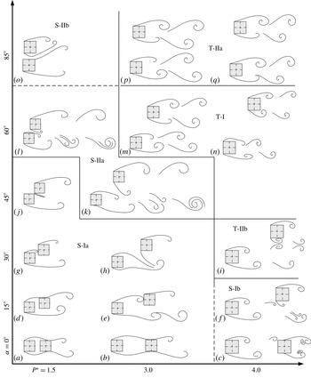
Each flow mode is associated with rather unique shear layer separations and interactions, which may be for simplicity referred to as the initial conditions. A total of 10 distinct initial conditions have been identified. Figure 15 provides an overview on the dependence of the flow structure mode on the initial conditions, schematically sketched, and also
 $P^{\ast }$
and
 ${\it\alpha}$
. The flow structure mode is characterized not only by a variation in
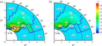
 $St$
, as discussed in § 5, but also by the ratio
 ${\it\gamma}$
of
 $St$
in the upstream-cylinder-generated vortex street to that behind the other cylinder. As a matter of fact, the dependence of
 ${\it\gamma}$
on
 $P^{\ast }$
and
 ${\it\alpha}$
(figure 16), measured at
 $x^{\ast }=4$
and 10, exhibits quite good correlation to the flow classification (cf. figure 6). For example,
 ${\it\gamma}>1$
at
 $x^{\ast }=4$
(figure 16
a) but
 ${\it\gamma}=1$
at
 $x^{\ast }=10$
(figure 16
b) for S-IIa, indicating the merging of two streets of distinct
 $St$
into one. On the other hand,
 ${\it\gamma}$
remains unchanged from
 $x^{\ast }=4$
to 10 for T-I (figure 16
a,b). Further discussion on individual flow modes is presented below.
Sketches of possible flow structures: mode S-Ia (a,b,d,e,g,h,j); S-Ib (c,f); S-IIa (k, l); S-IIb (o); T-I (n,m); T-IIa (p,q); T-IIb (i). Initial conditions (i): (a,b), (ii): (d), (iii): (e,g), (iv): (h,j), (v): (c), (vi): (f), (vii): (k,l), (viii): (o), (ix): (m,n) and (x): (p,q).

Isocontours of the ratio
 ${\it\gamma}$
of
 $St$
behind the upstream cylinder to that behind the downstream: (a)
 $x^{\ast }=4$
and (b) 10. The
 $\text{contour increment}=0.2$
.
 $Re=1.3\times 10^{4}$
.

Mode S-Ia. Being close enough, the two cylinders interact with each other largely via shear layers or the rather weak gap flow. Four distinct initial conditions are observed. (i) At
 $P^{\ast }<3.75$
and
 ${\it\alpha}=0^{\circ }$
, both shear layers separated from the upstream cylinder reattach on the side surface of and interact with the shear layers around the downstream cylinder (figure 15
a,b). Reattachment occurs near the trailing and leading corners of the surface at smaller (figure 15
a) and larger
 $P^{\ast }$
(figure 15
b), respectively. (ii) For
 ${\it\alpha}\geqslant 5^{\circ }$
only the upper shear layer reattaches (figure 15
d). The corresponding
 $St$
is 0.12–
 $0.13\lesssim St_{0}$
(figure 6) as reattachment slows down the shear layer velocity. A shift in the reattachment position from the trailing to leading corner causes a decrease in
 $St$
. (iii) For larger
 ${\it\alpha}$
or
 $P^{\ast }$
, the upper shear layer impinges on the front surface of the downstream cylinder (figure 15
e,g). Impingement near the lower leading corner (figure 15
g) corresponds to a smaller
 $St$
than that near the upper leading corner (figure 15
e). Since the shear layer impingement delays the process of vortex shedding from the downstream cylinder,
 $St=0.08{-}0.12$
(figure 6) is smaller than that associated with shear layer reattachment on the side surface. The shear layer impingement on the downstream cylinder not only delays but also weakens the vortex shedding from the downstream cylinder. The degree of weakening is dependent on the size of the second cylinder. For example, a small rod placed in the shear layer around a large cylinder may suppress vortex shedding from the large cylinder (Igarashi & Tsutsui Reference Igarashi and Tsutsui1989; Strykowski & Sreenivasan Reference Strykowski and Sreenivasan1990; Sakamoto, Tan & Haniu Reference Sakamoto, Tan and Haniu1991). Given an adequately large size, the downstream cylinder may suppress the shedding from the upstream cylinder, though acting as a bluff body shedding vortices in its wake. (iv) At larger
 ${\it\alpha}$
, the upper shear layer from the upstream cylinder and the lower shear layer from the downstream cylinder flow through the gap, acting as a base bleed (figure 15
h,j). This provides additional momentum in the near wake and prolongs the formation length of vortices separated from the free-stream or outer sides of the cylinders (Igarashi Reference Igarashi1978; Franssona, Koniecznyb & Alfredsson Reference Franssona, Koniecznyb and Alfredsson2004) Due to an increased effective bluff width,
 $St$
is only 0.07–0.8 albeit increased by the base bleed.
Mode S-Ib. As
 $P^{\ast }$
is increased at a small
 ${\it\alpha}$
, the shear layers separated from the upstream-cylinder roll up, forming vortices, before reaching the downstream cylinder (figure 15
c,f). Two distinct initial conditions are found. (v) The upstream-cylinder-generated vortices interact with the shear layers around the downstream cylinder or impinge on its front surface at
 ${\it\alpha}<10^{\circ }$
(figure 15
c). This interaction forces a coupling between the upstream-cylinder-generated vortices and vortex shedding from the downstream cylinder, producing the binary vortices behind the downstream cylinder as observed by Papaioannou et al. (Reference Papaioannou, Yue, Triantafyllou and Karniadakis2008). (vi) For
 ${\it\alpha}\geqslant 10^{\circ }$
, the vortices only in the upper row interact with vortex shedding from the downstream cylinder, forming two closely approaching counter-rotating vortices, which are enveloped by the vortex shed from the free-stream side of the upstream cylinder (figure 15
f). Again, the frequencies of vortex shedding from both cylinders are identical, with
 $St=0.11{-}0.12$
(figure 6). The presence of the downstream cylinder reduces the convective velocity of the vortices from the upstream cylinder, resulting in a smaller
 $St$
for the upstream-cylinder-generated vortices.
S-IIa. This mode occurs at intermediate
 ${\it\alpha}$
and small
 $P^{\ast }$
with an initial condition (vii). The gap gains adequate room so that both inner shear layers may squeeze through and roll up in a synchronized manner. Under the influence of the gap flow, the two counter-rotating vortices, characterized by low momentum, move together and swerve to the upstream cylinder (figure 15
k,l), producing one narrow and one wide street of high and small
 $St$
, respectively, in the immediate downstream vicinity of the cylinders. The two counter-rotating vortices interact vigorously with the vortex separated from the free-stream side of the upstream cylinder. The interaction between the three vortices may occur in two ways, that is, either both gap vortices are enveloped simultaneously by the other vortex (figure 15
l) or the nearer gap vortex is enveloped first and then the other gap vortex follows suit (figure 15
k). Obviously, the narrow street survives longer in the latter case. Another interaction is also observed in the wake of two circular cylinders, where only part of the gap vortex from the downstream cylinder and the other gap vortex are enveloped by the free-stream side vortex, termed as vortex pairing, splitting and enveloping by Sumner et al. (Reference Sumner, Price and Paidoussis2000). The three vortices merge into one, forming a wide asymmetrical wake at
 $x^{\ast }>7$
with the vortex separated from the free-stream side of the downstream cylinder. Therefore,
 ${\it\gamma}$
is 1.3–3.8 at
 $x^{\ast }=4$
but changes to 1.0 at
 $x^{\ast }=10$
(figure 16), with its maximum at
 $P^{\ast }=2.0$
and
 ${\it\alpha}=55^{\circ }$
.
Mode S-IIb. The initial condition (viii) is found for the first time at large
 ${\it\alpha}$
and small
 $P^{\ast }$
(figure 15
o). Due to the presence of a considerable gap passage, the shear layer separated from the downstream cylinder interacts with the shear layer around the upstream cylinder and is forced to swerve to the downstream cylinder. Furthermore, the upper shear layer around the upstream cylinder separates from the downstream corner. Thus, one wide and one narrow street are observed behind the upstream and downstream cylinders, respectively, as opposed to S-IIa. Yet, vigorous interactions between the gap and free-stream side vortices lead to the survival of only the wide street downstream. The
 ${\it\gamma}$
is 0.35–0.45 at
 $x^{\ast }=4$
but rises to 1.0 at
 $x^{\ast }=10$
(figure 16).
Mode T-I. As
 ${\it\alpha}$
or
 $P^{\ast }$
rises beyond its counterpart for S-II, the gap and free-stream side vortices cannot be merged with a large lateral separation between the two inner rows of vortices (figure 15
m,n). However, the presence of a downstream cylinder acts to produce a blockage, squeezing the street behind the upstream cylinder. As is well known, the wake of a single cylinder placed in a wind tunnel may experience a blockage effect if the separation between the cylinder and tunnel walls is not adequately large (Farrel & Blessmann Reference Farrel and Blessmann1983; Singka & Sinhamahapatra Reference Singka and Sinhamahapatra2010). This effect produces a narrower wake and hence larger
 $St$
(West & Apelt Reference West and Apelt1982). The gap flow and hence shear layers between the cylinders are slightly inclined toward the upstream cylinder. Such an initial condition (ix) produces a slightly narrower street behind the upstream cylinder than that behind the downstream cylinder. The two streets persist beyond
 $x^{\ast }=10$
with a difference in
 $St$
. The
 ${\it\gamma}$
is 3.3–1.1, depending on
 $P^{\ast }$
and
 ${\it\alpha}$
but not on
 $x^{\ast }$
(figure 16).
Mode T-IIa. As
 ${\it\alpha}$
exceeds
 $72.5^{\circ }$
, the two cylinders are approximately side-by-side arranged given
 $P^{\ast }>2.75$
, and the blockage effect of the downstream cylinder on the street behind the upstream cylinder is negligibly small. Under this initial condition (x), the shear layers around the two cylinders roll up, either inphased or antiphased, forming two streets of essentially the same width (figure 15
p,q) and
 ${\it\gamma}=1.0$
(figure 16).
Mode T-IIb. Given
 ${\it\alpha}=17.5^{\circ }{-}42.5^{\circ }$
and
 $P^{\ast }>3.75$
, the downstream cylinder is both laterally and longitudinally far enough from the upstream cylinder, producing again a negligibly small blockage effect. Initial condition (x) applies. T-IIb resembles T-IIa in terms of the nature of the streets and its
 ${\it\gamma}$
is 1.0 (figure 16). But
 $St$
is slightly smaller, 0.11–0.13, than
 $St_{0}$
or that
 $(=St_{0})$
for T-IIa (figure 6). There is a coupling between the inner vortices of the two streets, which triggers vortex shedding from the downstream cylinder, accounting for the same
 $St$
in the two streets (figure 15
i).
7 Conclusions
A systematic study has been conducted on the wake of two staggered square cylinders based on extensive measurements at
 $Re=1.3\times 10^{4}$
, using various techniques. The
 $P^{\ast }$
and
 ${\it\alpha}$
ranges examined are 1.5–5.0 and
 $0^{\circ }{-}90^{\circ }$
, respectively. Four distinct flow regimes, i.e. S-I, S-II, T-I and T-II, are identified based on the flow structure,
 $St$
and their downstream evolution over
 $x^{\ast }=4{-}15$
. The study of this highly complicated flow is then reduced to the understanding of flow in the four regimes.
Mode S-I occurs largely at
 ${\it\alpha}<17.5^{\circ }{-}45.7^{\circ }$
, depending on
 $P^{\ast }$
. This mode is characterized by only one Kámán vortex street of a single
 $St\,(=0.07{-}0.13<St_{0})$
and is further divided into S-Ia and S-Ib in view of a great disparity in the vortex strength and very different formation processes of gap vortices. S-Ia is associated with two closely separated cylinders (
 $P^{\ast }<3.75$
,
 ${\it\alpha}=0^{\circ }{-}47.5^{\circ }$
). The outer shear layers shed alternately from the two cylinders, forming a single vortex street behind the cylinders with
 ${\it\gamma}=1.0$
. Nevertheless, the inner shear layer separated from the upstream cylinder plays an important role in fluid dynamics. This layer may reattach on the side surface or impinge on the front surface of the downstream cylinder or go through the gap; the corresponding
 $St$
is 0.12–0.13, 0.08–0.12 and 0.07–0.08, respectively. The vortex strength is slightly lower than that in an isolated single cylinder wake. S-Ib occurs at large
 $P^{\ast }\,({>}3.75)$
and small
 ${\it\alpha}\,({<}17.5^{\circ })$
, where vortices, shed alternately from the two sides of the upstream cylinder, impinge on the downstream cylinder and act to trigger vortex shedding from the downstream cylinder at
 $St=0.11{-}0.12$
. The vortex impingement results in a great reduction in the vortex strength, compared with that of S-Ia.
Mode S-II is associated with large
 ${\it\alpha}\,({>}17.5^{\circ })$
and small
 $P^{\ast }\,({<}3.75)$
, where the lateral separation between the cylinders is adequately large, so that two counter-rotating vortices are generated in the shear layers through the gap and are deflected toward one of the cylinders, producing a narrow vortex street of higher
 $St$
and a wide street of smaller
 $St$
. The two vortex streets interact vigorously with each other and merge into one single vortex street of the low
 $St$
at
 $x^{\ast }>7$
. S-II is divided into S-IIa and S-IIb, depending on the mechanisms the gap flow is deflected. In S-IIa, the gap flow is deflected toward the upstream cylinder, squeezed by the downstream cylinder at a relatively large
 $P^{\ast }$
or directed by the gap flow passage with a short length at a relatively small
 $P^{\ast }$
. In S-IIb, the gap flow is swerved toward the downstream cylinder when the gap flow passage is relatively long and the gap flow is directed toward the downward cylinder due to the occurrence of the hit-and-bounce phenomenon. The
 ${\it\gamma}$
is 1.3–3.8 for S-IIa and 0.35–0.45 for S-IIb at
 $x^{\ast }<7$
but becomes 1.0 for both cases at
 $x^{\ast }>7$
.
Mode T-I comes to existence at
 $P^{\ast }>1.75$
and
 $32.5^{0}<{\it\alpha}<90^{\circ }$
. This mode is characterized by one narrow street of higher
 $St$
and one wide street of lower
 $St$
behind the upstream and downstream cylinder, respectively. However, unlike S-II, the two streets retain their identities, without merging into one, until at least
 $x^{\ast }=15$
presently examined. The wide street is associated with larger vortex strength than the narrow street.
 $St$
in the narrow street decreases from 0.22 to 0.13 as
 $P^{\ast }$
and/or
 ${\it\alpha}$
are increased, while that in the wide street increases from 0.08 to 0.13, resulting in
 ${\it\gamma}=3.3{-}1.1$
, which does not vary with
 $x^{\ast }$
.
Mode T-II is characterized by two streets of the same width, with
 ${\it\gamma}=1.0$
. T-II is divided into T-IIa and T-IIb. The former emerges at
 ${\it\alpha}>72.5^{\circ }$
and
 $P^{\ast }>2.75$
. The same
 $St\approx St_{0}\,(=0.134)$
results from coupled vortex shedding from the two cylinders, predominantly antiphased, though the inphased shedding is also observed. The latter arises at
 $17.5^{\circ }<{\it\alpha}<42.5^{\circ }$
and
 $P^{\ast }>3.75$
and appears the same as T-IIa, except with a slightly lower
 $St$
. The vortices separated from the inner side surface of the upstream cylinder are advected downstream, acting to trigger vortex shedding from the downstream cylinder, leading to the same
 $St$
in the two streets.
A total of ten initial conditions are identified, each characterized by a unique interaction between the four shear layers and two cylinders. Initial condition (i) is characterized by reattachment of both shear layers, separated from the upstream cylinder, on the side surface of the downstream cylinder; but only the upper shear layer reattachment takes place for initial condition (ii). The upper shear layer impinges upon the front surface of the downstream cylinder in initial condition (iii) but fails in condition (iv) where this shear layer makes its way through the gap, joining the lower shear layer from the downstream cylinder. While the upstream-cylinder-generated vortices interact with the shear layers around or impinge upon the front surface of the downstream cylinder in condition (v), only those of the upper row interact directly with vortex shedding from the downstream cylinder in condition (vi). Both inner shear layers veer to the upstream cylinder and form synchronized counter-rotating vortices, resulting in condition (vii), but swerve to the downstream cylinder in condition (viii). The deflection of both inner shear layers or gap flow is markedly reduced in condition (ix) and is even no longer biased in condition (x). Initial conditions (i) to (iv) result in Mode S-Ia, (v) and (vi) lead to mode S-Ib, while (vii), (viii) and (ix) account for modes S-IIa, S-IIb and T-I, respectively. However, initial condition (x) is responsible for modes T-IIa and T-IIb.
Acknowledgements
Authors wish to acknowledge support given to them from NSFC through grants 51421063 and 11302062, and from Scientific Research Fund of Shenzhen Government through grants KQCX2014052114430139, KQCX20130627094615415, KQCX2014052114423867 and JCYJ20120613145300404.