1 Introduction
Amorphic complexity was introduced in [Reference Fuhrmann and Gröger21–Reference Fuhrmann, Gröger, Jäger and Kwietniak23] as a complexity measure for topological dynamical systems
 $(\mathbb {X},G)$
, where
 $\mathbb {X}$
is a compact space with some metric d and G a locally compact,
 $\sigma $
-compact Abelian group acting on
 $\mathbb {X}$
by homeomorphisms. The intention was to provide a finer classification tool for the abundance of dynamical systems with vanishing entropy. Following [Reference Fuhrmann and Gröger21–Reference Fuhrmann, Gröger, Jäger and Kwietniak23], see also [Reference Bruin16, Reference Petersen32], for any
 $\delta> 0$
and
 $x,y \in \mathbb {X}$
, we define the set
 $$ \begin{align} \varDelta^{}_{\delta}(x,y) = \{t \in G : d(x+t,y+t) \geqslant \delta \} \end{align} $$
and use
 $D^{}_{\hspace {-0.5pt}\delta }(x,y)$
to denote the (upper) asymptotic density of the set
 $\varDelta ^{}_{\delta }(x,y)$
, measured with respect to some (arbitrary, but fixed) Følner sequence
 $\mathcal {F} = \{ {F}_n \}_{n\in \mathbb {N}}$
,
 $$ \begin{align} D^{}_{\hspace{-0.5pt}\delta}(x,y) = \operatorname{{\mathrm{dens}}} ( \varDelta^{}_{\delta}(x,y) ) = \limsup_{n \rightarrow \infty} \frac{|\varDelta^{}_{\delta}(x,y) \cap {F}_n|}{|{F}_n|}. \end{align} $$
Here,
 $| \cdot |$
denotes the Haar measure of G, sometimes also denoted by
 $\theta ^{}_{G}$
. Then, a set
 $S \subseteq \mathbb {X}$
is
 $(\delta ,\nu )$
-separated if, for all
 $x,y \in S$
with
 $x \ne y$
, we have
 $D^{}_{\hspace {-0.5pt}\delta }(x,y) \geqslant \nu $
. Denoting by
 $\mathrm {Sep\hspace {0.5pt}}(\mathbb {X},\delta ,\nu )$
the maximal cardinality of any
 $(\delta ,\nu )$
-separated subset of
 $\mathbb {X}$
, the (upper) amorphic complexity was defined as
 $$ \begin{align} \text{ac}(\mathbb{X},G) \mathrel{\mathop:}= \sup_{\delta>0} \limsup_{\nu {\scriptscriptstyle\searrow} 0} \frac{\log ( \mathrm{Sep\hspace{0.5pt}}(\mathbb{X},\delta,\nu))}{-\!\log(\nu)}. \end{align} $$
This is analogous to a box counting dimension if
 $\mathrm {Sep\hspace {0.5pt}} ( \mathbb {X}, \delta , \nu )$
is regarded as the maximum number of disjoint open balls of diameter
 $\nu $
that one can squeeze into
 $\mathbb {X}$
. Under reasonable assumptions on G, it turned out that
 $\mathrm {Sep\hspace {0.5pt}}(\mathbb {X},\delta ,\nu )$
, and hence
 $\text {ac}(\mathbb {X},G)$
, can only be finite if
 $(\mathbb {X},G)$
has vanishing topological entropy [Reference Fuhrmann, Gröger, Jäger and Kwietniak23].
In view of the general notions in dynamics, including the discussions in [Reference Bruin16, Reference Petersen32], we stress the following. Amorphic (or amorphous) systems are usually understood to have positive entropy, both in mathematics and in physics. In a sense, amorphic systems and systems for which amorphic complexity is meaningful (finite) are at opposite ends of the complexity spectrum. In fact, for the important case of a minimal dynamical system
 $(\mathbb {X},G)$
, the separation numbers
 $\mathrm {Sep\hspace {0.5pt}}(\mathbb {X},\delta ,\nu )$
are finite precisely when
 $(\mathbb {X},G)$
has topological pure-point spectrum, that is, if it is uniquely ergodic and has pure point dynamical spectrum with continuous eigenfunctions [Reference Fuhrmann, Gröger, Jäger and Kwietniak23]. Hence, systems with pure-point spectrum are in many respects much more like (aperiodic) crystals, not like amorphic systems. Calling a complexity measure that is meaningful only for such systems amorphic seems to be misleading. In view of its definition and the fact that this quantity has the flavour of a dimension, we therefore propose to call it orbit separation dimension (
 $\mathrm {OSD}$
) in the rest of this paper and denote it by
 $\mathrm {OSD}(\mathbb {X},G)$
.
The concept itself, however, is an interesting and powerful tool, which allows, both theoretically and practically, to analyse topological dynamical systems (TDS). In the context of symbolic dynamical systems, it has been studied for constant-length substitutions in [Reference Fuhrmann and Gröger21], while several classes of model sets were covered in [Reference Fuhrmann, Gröger, Jäger and Kwietniak23]. In this paper, we apply it to spaces
 $\mathbb {X}$
of self-similar aperiodic tilings of
 $\mathbb {R}\hspace {0.5pt}^d$
that are generated by a primitive inflation rule. Such inflation tilings constitute a rich class of interesting examples whose translation dynamical systems are automatically strictly ergodic and share other nice properties. We expect that some transfer will also be possible to systems of self-affine tilings, which are generally more complicated and will certainly need further investigations.
Due to the self-similarity, tools are available [Reference Solomyak37] to determine whether the spectrum of the translation action is pure-point—a necessary requirement for finite
 $\mathrm {OSD}$
. If that is the case, these systems are almost
 $1$
-to-
 $1$
extensions of their underlying maximal equicontinuous factor (MEF) and all their eigenfunctions can be chosen continuous [Reference Solomyak39] (for a discussion of the MEF in our context, see [Reference Barge and Kellendonk15]). In a similar way, the self-similarity can also be used to determine the
 $\mathrm {OSD}$
exactly in many cases, which provides an invariant under topological conjugation for distinguishing tiling spaces which are otherwise difficult to tell apart. The class of primitive inflation tilings is therefore an ideal playground to study and apply
 $\mathrm {OSD}$
, where it is both non-trivial and practically computable.
The remainder of this paper is organized as follows. Before we start with the main topic, §2 collects some facts and properties of mean equicontinuity and primitive inflation tilings. In §3, we then construct a transversal to the continuous group action. The reason is that this transversal already determines the
 $\mathrm {OSD}$
and can be constructed as the fixed point of a graph-directed iterated function system (GIFS). The latter then allows us to compute the
 $\mathrm {OSD}$
in terms of a discrepancy inflation in §4.
Before we illustrate, in §7, the concepts developed in this paper with an extensive collection of examples, we take a closer look at product tilings in §5, and briefly comment on the relation between
 $\mathrm {OSD}$
and the dimension of the window boundary of cut-and-project sets in §6. We end the paper with some concluding remarks in §8.
2 Preliminaries
Let us collect some results on mean equicontinuity of a dynamical system and its relation to
 $\mathrm {OSD}$
; see [Reference Fuhrmann and Gröger21, Reference Fuhrmann, Gröger, Jäger and Kwietniak23, Reference Fuhrmann, Gröger and Lenz24] for details. We do not deal with the most general case here, but constrain ourselves to G being Abelian, which simplifies things considerably. Also, in view of our tiling applications, we assume the dynamical system to be strictly ergodic.
So, we have a compact metric space
 $\mathbb {X}$
with metric d and a locally compact, second countable Abelian group G which acts continuously on
 $\mathbb {X}$
by homeomorphisms, thereby defining a TDS
 $(\mathbb {X},G)$
. We write the action of G additively. A Følner sequence
 ${\mathcal {F} = (F_n)_{n\in \mathbb {N}}}$
is a sequence of non-empty compact subsets
 $F_n$
of G such that, for all
 $g \in G$
,
 $$ \begin{align*} \lim_{n\to\infty} \frac{|(F_n+g)\triangle F_n|}{|F_n|} = 0 , \end{align*} $$
where
 $\triangle $
refers to the symmetric difference. Note that, for G Abelian, there is no need to distinguish between left and right Følner sequences. Given a Følner sequence
 $\mathcal {F}$
, we say that
 $(\mathbb {X},G)$
is (Besicovitch)
 $\mathcal {F}$
-mean equicontinuous if, for all
 $\varepsilon>0$
, there exists
 $\delta _\varepsilon>0$
such that
 $$ \begin{align} D^{}_{\hspace{-0.5pt}\mathcal{F}}(x,y) \mathrel{\mathop:}= \limsup_{n\rightarrow\infty} \frac{1}{|F_n|}\int_{F_n} d(x+t,y+t)\,{\mathrm{d}}\theta^{}_{G}(t) < \varepsilon \end{align} $$
for all
 $x,y\in \mathbb {X}$
with
 $d(x,y)<\delta _\varepsilon $
, where the integration is with respect to the Haar measure of G. Note that
 $D^{}_{\hspace {-0.5pt}\mathcal {F}}$
is not a metric, but a pseudometric on
 $\mathbb {X}$
.
There is also the notion of (Weyl) mean equicontinuity (or just mean equicontinuity), which is equicontinuity with respect to the pseudometric
 $D_{{}_{\mathrm {W}}} (x,y) \mathrel {\mathop :}= \sup _{\hspace {-0.5pt}\mathcal {F}}D^{}_{\hspace {-0.5pt}\mathcal {F}}(x,y)$
, where the supremum is taken over all Følner sequences, making
 $D_{{}_{\mathrm {W}}}$
manifestly independent of any Følner sequence. However, it turns out that, in the Abelian case, Weyl mean equicontinuity and Besicovitch
 $\mathcal {F}$
-mean equicontinuity for any Følner sequence
 $\mathcal {F}$
are actually equivalent; compare [Reference Fuhrmann, Gröger and Lenz24, Theorem 1.3]. With these notions, we can recall the following result from [Reference Fuhrmann and Gröger21, Reference Fuhrmann, Gröger, Jäger and Kwietniak23, Reference Fuhrmann, Gröger and Lenz24].
Theorem 2.1. Suppose
 $(\mathbb {X},G)$
is a minimal TDS with G Abelian and let
 $\mathcal {F}$
be any Følner sequence. Then, the following properties are equivalent.
-
•
 $(\mathbb {X},G)$
is Besicovitch
$\mathcal {F}$
-mean equicontinuous.
-
•
$(\mathbb {X},G)$
is Weyl mean equicontinuous. -
•
$(\mathbb {X},G)$
has a unique ergodic measure
$\mu $
and
$(\mathbb {X},G,\mu )$
has pure-point dynamical spectrum with continuous eigenfunctions. -
• The separation numbers
$\mathrm {Sep}(\mathbb {X},\delta ,\nu )$
are finite.


Recall that the
 $\mathrm {OSD}$
of mean equicontinuous, minimal dynamical systems does not depend on the choice of the Følner sequence [Reference Fuhrmann, Gröger, Jäger and Kwietniak23, Theorem 1.2]. Since we are only concerned with such systems throughout this work, the choice of
 $\mathcal {F}$
will be immaterial.
We also note that, for mean equicontinuous dynamical systems
 $(\mathbb {X},G)$
, the factor map to the MEF can be obtained by identifying points with vanishing distance in the pseudometric
 $D_{{}_{\mathrm {W}}}$
. More precisely, we consider the equivalence relation given by
 $$ \begin{align} x \sim y \Longleftrightarrow D_{{}_{\mathrm{W}}}(x,y) = 0, \end{align} $$
called the equicontinuous structure relation. The equivalence class corresponding to x is denoted by
 $[x]$
and
 $D_{{}_{\mathrm {W}}}$
naturally defines a metric on the quotient space
 $[\mathbb {X}] = \mathbb {X}/{\sim }$
via
 $D_{{}_{\mathrm {W}}}( [x], [y] ) \mathrel {\mathop :}= D_{{}_{\mathrm {W}}}(x,y)$
. It is easily checked that this is well defined. For every subset
 $S \subseteq \mathbb {X}$
, we also use the notation
 $$ \begin{align*} [S] = \{ [x] : x \in S \}. \end{align*} $$
Since the pseudometric
 $D_{{}_{\mathrm {W}}}$
is invariant under translations, the same holds for the corresponding equivalence relation. This shows that the group action
 $$ \begin{align*} [x] \longmapsto [x]+t \mathrel{\mathop:}= [x+t] \end{align*} $$
is well defined on the quotient space, thus turning
 $( [\mathbb {X}],G )$
into another TDS. By construction, the (quotient) map
 $$ \begin{align*} \pi \colon \mathbb{X} \xrightarrow{\quad} [\mathbb{X}], \quad x \mapsto [x] \end{align*} $$
intertwines (or semi-conjugates) the action of G on the two spaces. Since we assume that
 $(\mathbb {X},G)$
is mean equicontinuous, the action of
 $\pi $
is continuous and hence defines a factor map from one TDS onto another. In this situation, it is also known that
 $([\mathbb {X}],G)$
coincides with the MEF of
 $(\mathbb {X},G)$
; see [Reference Fuhrmann, Gröger and Lenz24, Proposition 3.13], as well as [Reference Aujogue, Barge, Kellendonk, Lenz, Kellendonk, Lenz and Savinien5, Reference Auslander6] for background.
As already indicated, our systems of interest are spaces of primitive inflation tilings and their translation dynamical systems. We will therefore confine ourselves to
 $G=\mathbb {R}\hspace {0.5pt}^d$
(or to some discrete subgroup thereof, such as
 $\mathbb {Z}\hspace {0.5pt}^d$
). In the remainder of this section, we give a brief description of the setup and the basic properties. For background, we refer to [Reference Baake and Grimm11].
A tiling is a covering of
 $\mathbb {R}\hspace {0.5pt}^d$
with tiles, which are compact sets each of which is the closure of its interior, and which are supposed to overlap at most on their boundaries. We only consider the case of regular tiles, that is, tiles with a boundary of Lebesgue measure
 $0$
. Tiles may also carry an extra label to distinguish tiles of different type, but having congruent support (or shape). We assume that, up to translation by elements of G, there are only finitely many tile types, called prototiles. We also require that tiles may be joined in finitely many ways only. To make this more precise, if
 $B_{r} (a)$
is the closed ball of radius r centred at a, we call the collection of all those tiles in a tiling x which intersect such a ball an r-patch, written as
 $x \sqcap B_{r} (a)$
. We require that, up to translation, the number of different r-patches is finite for any radius r. This property is called finite local complexity (FLC).
On the space of all tilings constructed from a given set of prototiles, we have a metric, known as the tiling metric
 $d(x^{}_1 , x^{}_2 )$
, which is defined as
 $$ \begin{align*} d (x^{}_1 ,x^{}_2) \mathrel{\mathop:}= \min \{ \widetilde{d}(x^{}_1 , x^{}_2), 2^{-1/2} \}, \end{align*} $$
where
 $$ \begin{align*} \widetilde{d}(x_1,x_2) = \inf \{ \varepsilon> 0 : &\text{ there exists } t^{}_1, t^{}_2 \in B_\varepsilon(0)\\& \text{ with } (x^{}_1 - t^{}_1) \sqcap B_{1/\varepsilon}(0) = (x^{}_2 - t^{}_2) \sqcap B_{1/\varepsilon}(0) \}. \end{align*} $$
In words, to be
 $\varepsilon $
-close, the tilings must exactly agree in a ball of radius
 $1/\varepsilon $
around the origin, possibly after some
 $\varepsilon $
-small rigid translations [Reference Solomyak37]. The cap at
 $2^{-1/2}$
is necessary for the triangle relation to hold [Reference Lee, Moody and Solomyak28]. The topology induced by the tiling metric is called the local topology; compare [Reference Baake and Grimm11]. The orbit closure of an FLC tiling in the local topology is compact. The group
 $\mathbb {R}\hspace {0.5pt}^d$
acts continuously on it by translation. We thereby obtain a topological tiling dynamical system
 $(\mathbb {X},\mathbb {R}\hspace {0.5pt}^d)$
, or TTDS for short. For the tilings we consider, these dynamical systems will be strictly ergodic, so that the tiling space can be constructed as the closure of the
 $\mathbb {R}\hspace {0.5pt}^d$
-orbit of any of its elements.
We further assume that our tiling space is invariant under a primitive inflation rule with a uniform scaling factor. In this procedure, a tile, patch of tiles or an entire tiling is scaled by a factor
 $\unicode{x3bb}>1$
(which necessarily is an algebraic integer; compare [Reference Baake and Grimm11, Theorem 2.4] and references given there) and the scaled tiles are then dissected in a unique way into tiles of the original size. Starting with a single tile, by iterated inflation, and combined with translations, one can then generate larger and larger patches, and then (in the limit) tilings of the entire space. An inflation procedure is called primitive if it eventually produces, from any starting tile, a patch containing tiles of all types simultaneously. Primitive inflation rules have the property that all tilings they can generate are locally indistinguishable (LI), and hence members of the same tiling space, with strictly ergodic translation dynamics.
The case just described, where a scaled tile is replaced by a patch of tiles having the same support as the scaled tile, is called a stone inflation [Reference Baake and Grimm11]. The condition of matching supports can actually be relaxed to some extent, as long as tiles in a tiling are replaced by patches which still cover the whole space without (interior) overlaps. Then, there exists a stone inflation tiling which is mutually locally derivable (MLD, compare [Reference Baake and Grimm11]), often even with a combinatorially isomorphic inflation. MLD induces a topological conjugacy of the dynamical systems, with a conjugating map that is uniformly local.
If a tiling space consists of aperiodic tilings, each tiling has a unique predecessor under inflation, a property which is known as recognizability or unique composition [Reference Solomyak38]; this is the situation of a local inflation deflation symmetry (LIDS) in [Reference Baake and Grimm11]. If, moreover, the spectrum of the translation action with respect to the unique invariant measure on the tiling space
 $\mathbb {X}$
is pure point, all eigenfunctions are known to have continuous representatives [Reference Solomyak39]. The MEF is thus non-trivial, and the factor map to the MEF is known to be one-to-one almost everywhere (with respect to the Haar measure on the MEF) and uniformly bounded-to-one everywhere; compare [Reference Barge and Kellendonk15].
In view of Theorem 2.1, we may restrict our attention to those tiling dynamical systems that have pure-point dynamical spectrum. That is, for the remainder of this work, we assume that
 $(\mathbb {X},G)$
is a pure-point tiling dynamical system, generated by a primitive inflation rule
 $\varrho $
. To avoid trivialities, we further assume
 $(\mathbb {X},G)$
to be non-periodic. (In the fully periodic case, the dynamics is equicontinuous, resulting in vanishing
 $\mathrm {OSD}$
. More generally, by a refined argument of this type, no periodic direction contributes to the
 $\mathrm {OSD}$
.) In this case,
 $\varrho $
defines a homeomorphism on
 $\mathbb {X}$
that induces a map on the MEF via
 $$ \begin{align*} \varrho \colon [\mathbb{X}] \xrightarrow{\quad} [\mathbb{X}], \quad [x] \mapsto [\varrho(x)]. \end{align*} $$
This is a well-defined homeomorphism on
 $[\mathbb {X}]$
, compare [Reference Aujogue, Barge, Kellendonk, Lenz, Kellendonk, Lenz and Savinien5], which is consistent with set notation in the sense that
 $$ \begin{align} \varrho ( [x] ) = \{ \varrho(y) : y \in [x] \}. \end{align} $$
This partly justifies the slight abuse of notation in choosing the same symbol
 $\varrho $
for the induced map on the MEF. Now, our calculations of the
 $\mathrm {OSD}$
will rely on the observation that it coincides with the upper box counting dimension of (a subspace of) the MEF, equipped with an appropriate metric, as we explain next.
3 The transversal
As a first step, we define a transversal
 $\mathbb {X}^{}_{0} \subset \mathbb {X}$
to the TTDS
 $(\mathbb {X},\mathbb {R}\hspace {0.5pt}^d)$
, with the property that the set of translations
 $\{t \in \mathbb {R}\hspace {0.5pt}^d : \text { there exists } x\in \mathbb {X}^{}_{0} \text { with } x+t \in \mathbb {X}^{}_{0}\}$
is uniformly discrete (and, in general, no longer forms a group). Such a transversal, also called discrete hull, had already been used by Kellendonk [Reference Kellendonk25]. As we shall see, the use of a transversal will simplify the computation of the separation numbers
 $\mathrm {Sep\hspace {0.5pt}}(\mathbb {X},\delta ,\nu )$
significantly.
Remark 3.1. In the case where G is discrete, such as
 $\hspace {0.5pt} G=\mathbb {Z}\hspace {0.5pt}^d$
, the construction of a transversal can actually be omitted and the reader can continue directly after the proof of Corollary 3.8, with
 $\mathbb {X}^{}_{0}=\mathbb {X}$
. Conversely, a discrete group
 $\mathbb {Z}\hspace {0.5pt}^d$
can also be extended to
 $\mathbb {R}\hspace {0.5pt}^d$
via a standard suspension (with constant roof function), without changing the
 $\mathrm {OSD}$
; see [Reference Fuhrmann, Gröger, Jäger and Kwietniak23]. A discrete group
 $\hspace {0.5pt} G=\mathbb {Z}\hspace {0.5pt}^d$
naturally occurs for (symbolic) constant-length substitutions (
 $d=1$
) or for constant-shape block substitutions; compare [Reference Fuhrmann and Gröger21]. Standard suspensions of such systems are naturally isomorphic to inflation tilings where all tiles are congruent to d-dimensional unit cubes, which are then distinguished only by their type label. There are further generalizations, as one can see from the half-hex inflation, but we do not go into further details.
To construct the transversal, we need to define so-called control points for all tiles, which are special reference points with some extra properties. The control point of a single tile
 $\tau $
is denoted by
 $\mathrm {cp} (\tau )$
. Now, if two tiles
 $\tau $
,
 $\tau '$
of the same type occur in the same tiling x, they are translates of each other,
 $\tau = \tau ' + t$
, and we request that their control points then satisfy
 $\mathrm {cp}(\tau ) = \mathrm {cp}(\tau ') + t$
. Such a translation t is called a (tile) return vector. The
 $\mathbb {Z}\hspace {0.5pt}$
-span R of all return vectors is called the module of return vectors. Finally, the module of eventual return vectors is defined as
 $R_{\mathrm {ev}} \mathrel {\mathop :}= \bigcup _{n \in \mathbb {N}_0} \unicode{x3bb} ^{-n}R$
, so that
 $\unicode{x3bb} R_{\mathrm {ev}} = R_{\mathrm {ev}}$
. Note that
 $R_{\mathrm {ev}} = R$
if and only if the algebraic integer
 $\unicode{x3bb} $
is a unit. By construction, control points of tiles of the same type are separated by a vector in
 $R_{\mathrm {ev}}$
, but for tiles of different types, this is not automatically the case and must be required as an extra property. Finally, we require that the control point of a tile inflated by
 $\unicode{x3bb} $
coincides with the control point of one of its constituent tiles. The next result shows that control points with the required properties can always be chosen. Further useful requirements will be discussed as we proceed.
Lemma 3.2. For the tiles in a primitive inflation tiling with inflation factor
 $\unicode{x3bb} $
, it is possible to choose control points with the following properties.
-
(1) For any two tiles in the tiling, the difference of their control points is contained in the module
$R_{\mathrm {ev}}$
of eventual return vectors. -
(2) The control point
$\unicode{x3bb} \mathrm {cp}(\tau )$
of an inflated tile
$\unicode{x3bb} \tau $
coincides with the control point of one of its constituent tiles. -
(3) Distinct tiles have distinct control points.


Sketch of proof.
We essentially follow Kenyon [Reference Kenyon26]. For each tile
 $\tau $
of type i, we choose a fixed tile in its inflated version and call it the successor
 $\mathrm {succ}(\tau )$
of
 $\tau $
. We want the control point of
 $\tau $
to coincide with the control point of
 $\mathrm {succ}(\tau )$
after inflation,
 $\mathrm {cp} (\unicode{x3bb} \tau ) = \mathrm {cp} (\mathrm {succ} (\tau ))$
. Since
 $\mathrm {cp} (\unicode{x3bb} \tau ) = \unicode{x3bb} \hspace {0.5pt} \mathrm {cp} (\tau )$
, we certainly have
 $\mathrm {cp}(\tau ) \in \unicode{x3bb} ^{-1}\operatorname {{\mathrm {supp}}}(\mathrm {succ}(\tau ))$
. Now, also
 $\mathrm {succ}(\tau )$
has a successor,
 $\mathrm {succ}(\mathrm {succ}(\tau ))=\mathrm {succ}^2(\tau )$
, so that
 $\mathrm {cp}(\tau )$
must be contained also in
 $\unicode{x3bb} ^{-2}\operatorname {{\mathrm {supp}}}(\mathrm {succ}^2(\tau ))$
. Iterating this, we get
 $$ \begin{align*} \mathrm{cp}(\tau) \in \bigcap_{n\in\mathbb{N}}\unicode{x3bb}^{-n}\operatorname{{\mathrm{supp}}} (\mathrm{succ}^n(\tau)). \end{align*} $$
The latter set is non-empty and consists of a single point so that we have fixed the control points of all tile types. By construction, they satisfy requirement (2).
To fulfil also the first requirement, we observe that, for a primitive inflation rule with finitely many prototiles, there exists a power n of the inflation and a tile type i such that the nth inflation of each tile type contains a tile of type i. Choosing such a tile as successor produces control points satisfying also requirement (1), first for the nth power of the inflation, but these control points can also be used for the original inflation.
Finally, to avoid control points on a boundary, we may choose a suitable successor in the interior of an inflated tile, with positive distance to the boundary of the latter. This shows that requirement (3) can also be satisfied, without interference with the previous steps.
Remark 3.3. In some situations, it is desirable to require further properties of the control points. For instance, in one dimension, it would be convenient to choose the left endpoints of the tiles as control points, which may be in conflict with requirement (1), for instance outside the case of height
 $1$
in constant-length substitutions. This problem can be cured by passing to a tiling which is MLD to the original one, for instance by using a suitable return word encoding.
Remark 3.4. An important further requirement is that the control point set should be MLD with the tiling. Indeed, we should think of control points as carrying an extra label, which identifies the type of the tile a control point represents. In this sense, the set of control points
 $\mathrm {cp}(x)$
of a tiling x is a subset of
 $\mathbb {R}\hspace {0.5pt}^d \times S$
, with S the set of tile types. Such a set of labelled control points is MLD with the tiling it is derived from. Often, the extra label is not necessary, for instance if the tile type can be determined from the local neighbourhood of other control points. Thus, to avoid overloaded notation, we usually silently drop the type label from a control point when it is not needed.
In the following, we always assume that suitable control points have been chosen.
Definition 3.1. Suppose that control points according to Lemma 3.2 have been chosen. Denoting by
 $\mathrm {cp}(x)$
the set of control points of all tiles in a tiling x, we define the transversal
 $\mathbb {X}^{}_{0}\subset \mathbb {X}$
as
 $\mathbb {X}^{}_{0} = \{x\in \mathbb {X} : 0 \in \mathrm {cp}(x)\}$
.
Corollary 3.5. By construction, the transversal
 $\mathbb {X}^{}_{0}$
has the following properties.
-
(1) The set
$\{ t \in \mathbb {R}\hspace {0.5pt}^d : \text { there exists } x \in \mathbb {X}^{}_{0} \text { with } t \in \mathrm {cp}(x) \}$
is uniformly discrete, with a minimal distance
$\rho>0$
between distinct points. -
(2) The inflation rule maps
$\mathbb {X}^{}_{0}$
into itself.



Proof. The set of control points
 $\mathrm {cp}(x)$
of a primitive inflation tiling
 $x\in \mathbb {X}^{}_{0}$
with pure-point spectrum is necessarily a Meyer set [Reference Lee27]. As such, its difference set,
 $\varLambda = \mathrm {cp}(x) - \mathrm {cp}(x)$
, which by the minimality of the dynamics is independent of x, is uniformly discrete and in fact a Meyer set itself. Hence, the difference
 $p-q$
of any two control points
 $p\in \mathrm {cp}(x)$
and
 $q\in \mathrm {cp}(y)$
,
 $x,y\in \mathbb {X}^{}_{0}$
, is an element of
 $\varLambda - \varLambda $
, so that
 $|p-q|$
is either
 $0$
or uniformly bounded away from
 $0$
by a positive constant
 $\rho $
.
By property (2) of Lemma 3.2, the inflation maps control points to control points, which means
 $\unicode{x3bb} \mathrm {cp}(x)\subset \mathrm {cp}(x)$
. The tilings in
 $\mathbb {X}^{}_{0}$
are those with a control point at
 $0$
, so that
 $\mathbb {X}^{}_{0}$
is mapped into itself.
We now define the separation number
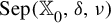 $\mathrm {Sep\hspace {0.5pt}}(\mathbb {X}^{}_{0},\delta ,\nu )$
as the maximal cardinality of any
 $(\delta ,\nu )$
-separated subset
 $S\subseteq \mathbb {X}^{}_{0}$
. Note that, since S is also a subset of
 $\mathbb {X}$
,
 $(\delta ,\nu )$
-separation is well defined also for any subset of
 $\mathbb {X}^{}_{0}$
. Clearly,
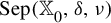 $\mathrm {Sep\hspace {0.5pt}}(\mathbb {X}^{}_{0},\delta ,\nu )$
is smaller than
 $\mathrm {Sep\hspace {0.5pt}}(\mathbb {X},\delta ,\nu )$
, but it is not much smaller, so that we can express the
 $\mathrm {OSD}$
in terms of
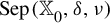 $\mathrm {Sep\hspace {0.5pt}}(\mathbb {X}^{}_{0},\delta ,\nu )$
.
However, before we do so, we note that, for
 $0<\delta '<\delta $
, we have
 $D^{}_{\hspace {-0.5pt}\delta '}(x,y)\geqslant D^{}_{\hspace {-0.5pt}\delta }(x,y)$
for any
 $x,y\in \mathbb {X}$
, and any
 $(\delta ,\nu )$
-separated set is also
 $(\delta ',\nu )$
-separated. Hence, in the definition of the
 $\mathrm {OSD}$
, we can restrict the supremum over
 $\delta $
to any interval
 $(0,\delta _0]$
with a conveniently chosen
 $\delta _0$
, without affecting the
 $\mathrm {OSD}$
.
Further, since
 $D^{}_{\hspace {-0.5pt}\delta }$
fails to be a pseudometric on
 $\mathbb {X}$
, we need to make use of the following property, which replaces the triangle relation.
Lemma 3.6. For
 $x,y,z\in \mathbb {X}$
and
 $\delta>0$
, we have
 $ D^{}_{2\delta }(x,z) \leqslant D^{}_{\hspace {-0.5pt}\delta }(x,y) + D^{}_{\hspace {-0.5pt}\delta }(y,z)$
.
Proof. By the triangle inequality for the metric d, we observe that
 $d(x+t,z+t)\geqslant 2\delta $
requires at least one of the relations
 $d(x+t,y+t)\geqslant \delta $
and
 $d(y+t,z+t)\geqslant \delta $
to hold. That is, if
 $t\in \varDelta ^{}_{2\delta }(x,z)$
, we need
 $t\in \varDelta ^{}_{\delta }(x,y)$
or
 $t\in \varDelta ^{}_{\delta }(y,z)$
. Hence,
 $$ \begin{align*} \varDelta^{}_{2\delta}(x,z) \subseteq \varDelta^{}_{\delta}(x,y) \cup \varDelta^{}_{\delta}(y,z). \end{align*} $$
Taking the upper density on both sides proves the claim.
Lemma 3.7. For any fixed
 $\delta $
with
 $0<\delta <\rho /2$
, with the
 $\rho $
from Corollary 3.5, there exists a constant
 $C_\delta $
such that, for all
 $\nu>0$
, one has
 $ \mathrm {Sep\hspace {0.5pt}}(\mathbb {X},2\delta ,\nu ) \leqslant C_\delta \mathrm {Sep\hspace {0.5pt}}(\mathbb {X}^{}_{0},\delta ,\nu ) $
.
Proof. For translations
 $t \in \mathbb {R}\hspace {0.5pt}^d$
with
 $|t|<\delta $
and any
 $x \in \mathbb {X}^{}_{0}$
, we have
 $d(x,x+t)<\delta $
. Then,
 $\varDelta ^{}_{\delta }(x,x+t)$
is the empty set and we have
 $D^{}_{\hspace {-0.5pt}\delta }(x,x+t) = 0$
. If we now compare
 $x^{}_1 + t^{}_1$
and
 $x^{}_2 + t^{}_2$
for
 $x^{}_i \in \mathbb {X}^{}_{0}$
and
 $t^{}_i \in \mathbb {R}\hspace {0.5pt}^d$
, Lemma 3.6 implies that
 $$ \begin{align*} D^{}_{2\delta}(x^{}_1 + t^{}_1 , x^{}_2 + t^{}_2 ) = D^{}_{2\delta}(x^{}_1 , x^{}_2 + t^{}_2 - t^{}_1 ) \leqslant D^{}_{\hspace{-0.5pt}\delta}(x^{}_1 , x^{}_2 ) + D^{}_{\hspace{-0.5pt}\delta}( x^{}_2 , x^{}_2 + t^{}_2 - t^{}_1 ). \end{align*} $$
If
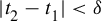 $|\hspace {0.5pt} t^{}_2 - t^{}_1 | < \delta $
, this reduces to
 $D^{}_{2\delta }(x^{}_1 + t^{}_1 , x^{}_2 + t^{}_2 ) \leqslant D^{}_{\hspace {-0.5pt}\delta }(x^{}_1 , x^{}_2 )$
. Hence,
 $x^{}_1 + t^{}_1$
and
 $x^{}_2 + t^{}_2$
can only be
 $(2\delta ,\nu )$
-separated if either
 $D^{}_{\hspace {-0.5pt}\delta }(x^{}_1 , x^{}_2 ) \geqslant \nu $
or
 $|t^{}_2 - t^{}_1| \geqslant \delta $
.
The set
 $\mathrm {cp}(x)$
of an FLC tiling x is a Delone set. There is a radius r such that the set of r-balls centred at control points covers
 $\mathbb {R}\hspace {0.5pt}^d$
, and due to the minimality of the dynamics, this radius r is the same for all
 $x\in \mathbb {X}^{}_{0}$
. Since the set
 $\{x+t : x\in \mathbb {X}^{}_{0}, t\in B_r (0)\}$
covers
 $\mathbb {X}$
completely, we see that the cardinality of any
 $(2\delta ,\nu )$
-separated set in
 $\mathbb {X}$
is bounded by
 $C_\delta \mathrm {Sep\hspace {0.5pt}}(\mathbb {X}^{}_{0},\delta ,\nu )$
, where
 $C_\delta $
is a constant of the order of
 $(r/\delta )^d$
, independent of
 $\nu $
.
The following result is an immediate consequence of Lemma 3.7.
Corollary 3.8.
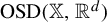 $\mathrm {OSD}(\mathbb {X},\mathbb {R}\hspace {0.5pt}^d)$
can be computed from the transversal
 $\mathbb {X}^{}_{0}$
as
 $$ \begin{align*} \mathrm{OSD}(\mathbb{X},\mathbb{R}\hspace{0.5pt}^d) = \sup_{\delta>0} \limsup_{\nu {\scriptscriptstyle\searrow} 0} \frac{\log ( \mathrm{Sep\hspace{0.5pt}}(\mathbb{X}^{}_{0},\delta,\nu))} {-\!\log(\nu)}. \end{align*} $$
This shows that we can work entirely with
 $\mathbb {X}^{}_{0}$
. It is worth noting that, on
 $\mathbb {X}^{}_{0}$
and for
 $\delta $
small enough,
 $D^{}_{\hspace {-0.5pt}\delta }$
is a pseudometric, which was not the case for
 $\mathbb {X}$
; compare Lemma 3.6. This is analogous to the discussion of symbolic dynamical systems in [Reference Fuhrmann and Gröger21, Lemma 6.2].
Lemma 3.9. For
 $\delta < \rho /2$
, where
 $\rho $
is the separation constant from Corollary 3.5,
 $D^{}_{\hspace {-0.5pt}\delta }$
is a pseudometric on
 $\mathbb {X}^{}_{0}$
.
Proof. Let
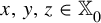 $x,y,z\in \mathbb {X}^{}_{0}$
. We show that, for distances below
 $\delta $
, the tiling metric d behaves like an ultra-metric on the simultaneous orbit of
 $x,y,z$
. More precisely, let
 $t\in \mathbb {R}\hspace {0.5pt}^d$
and assume
 $d(x-t,y-t)<\delta $
. Then, x and y agree on a ball of radius
 $1/\delta $
around t, after an at most
 $\delta $
-small rigid translation of one (or both) of the tilings. However, since x and y share a control point at the origin, all other control points either coincide or are at least a distance
 $\rho $
apart. Since
 $\delta < \rho /2$
, the tilings x and y must in fact agree exactly on the ball
 $B_{1/\delta }(t)$
.
By the same reasoning,
 $d(y-t,z-t)<\delta $
implies that y and z agree on
 $B_{1/\delta }(t)$
. Hence, the same holds for the pair
 $(x,z)$
, implying that
 $d(x-t,z-t)<\delta $
. Conversely, the inequality
 $d(x-t,z-t)\geqslant \delta $
now requires that one of
 $d(y-t,y-t)\geqslant \delta $
or
 ${d(y-t,z-t)\geqslant \delta }$
holds, which means that
 $$ \begin{align*} \varDelta^{}_{\delta}(x,z) \subseteq \varDelta^{}_{\delta}(x,y) \cup \varDelta^{}_{\delta}(y,z). \end{align*} $$
Taking the upper density on both sides gives
 $D^{}_{\hspace {-0.5pt}\delta }(x,z)\leqslant D^{}_{\hspace {-0.5pt}\delta }(x,y)+D^{}_{\hspace {-0.5pt}\delta }(y,z)$
.
In the same way, two tilings
 $x,y\in \mathbb {X}^{}_{0}$
can only be close in the tiling metric, for instance,
 $d(x,y)< \rho /2$
, if they exactly agree on some ball around the origin. This means that two tilings that are close must have some coincidences, that is, tiles which are shared by both. We introduce the following terminology.
Definition 3.2. For any two tilings
 $x,y\in \mathbb {X}^{}_{0}$
, we define the following two subsets of
 $\mathbb {R}\hspace {0.5pt}^d$
that, apart from a null set, are complements of each other.
-
(1) The coincidence set
$\mathrm {coin}(x,y)$
of x and y, which is the union of the supports of all tiles that do occur in both x and y. -
(2) The discrepancy set
$\mathrm {disc}(x,y)$
of x and y, which is the union of the supports of all tiles of x or y that do not occur in both tilings.


We have
 $\mathrm {coin} (x,y)=\overline {\mathbb {R}\hspace {0.5pt}^d\setminus \mathrm {disc}(x,y)}$
and
 $\mathrm {disc}(x,y)=\overline {\mathbb {R}\hspace {0.5pt}^d\setminus \mathrm {coin}(x,y)}$
. The two sets only intersect on their boundaries, which are null sets in our setting. With these concepts, we can now introduce another pseudometric on
 $\mathbb {X}^{}_{0}$
as follows.
Definition 3.3. For
 $x,y\in \mathbb {X}^{}_{0}$
and a fixed Følner sequence
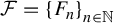 $\mathcal {F} = \{ F_n \}^{}_{n\in \mathbb {N}}$
, we set
 $$ \begin{align*} D(x,y) \mathrel{\mathop:}= \limsup_{n\rightarrow\infty} \frac{|\mathrm{disc}(x,y)\cap F_n|}{| F_n|}. \end{align*} $$
Note that D is indeed a pseudometric. It is obviously symmetric and positive semi-definite. Further, if a tile
 $\tau $
is not in
 $x \cap z$
, it cannot be both in
 $x \cap y$
and in
 $y \cap z$
. Hence, we get
 $\mathrm {disc}(x,z) \subseteq \mathrm {disc}(x,y) \cup \mathrm {disc}(y,z)$
and the triangle inequality follows.
Remark 3.10. As we already mentioned in the discussion following Theorem 2.1, the choice of the Følner sequence
 $\mathcal {F}$
is immaterial for the value of the
 $\mathrm {OSD}$
. It is worth pointing out that even the pseudometric D defined above does not depend on
 $\mathcal {F}$
for the systems at hand. Indeed, it was shown in [Reference Fuhrmann, Gröger and Lenz24, Theorem 1.2] that, for a mean equicontinuous, minimal system
 $(\mathbb {X},G)$
, the product system
 $(\mathbb {X} \hspace {0.5pt} {\hspace {0.5pt}\times \hspace {0.5pt}} \mathbb {X},G)$
is pointwise uniquely ergodic. Let
 $I(x,y)$
be the indicator function that takes the value
 $1$
if the pair
 $(x,y)$
has a discrepancy at the origin and
 $0$
otherwise. Then, we can write
 $D(x,y)$
as a Birkhoff average of I along the sequence
 $\mathcal {F}$
. Due to unique ergodicity of the orbit closure of
 $(x,y)$
, this average is independent of
 $\mathcal {F}$
. By the same reasoning, we see that the
 $\limsup $
in the definition of D can actually be replaced by a limit.
The pseudometric
 $D(x,y)$
is closely related to the pseudometric
 $D^{}_{\hspace {-0.5pt}\delta } (x,y)$
from equation (1.2).
Lemma 3.11. With respect to a fixed Følner sequence
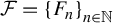 $\mathcal {F} = \{ F_n \}^{}_{n\in \mathbb {N}}$
, the pseudometrics
 $D(x,y)$
and
 $D^{}_{\hspace {-0.5pt}\delta } (x,y)$
, with
 $\delta \in (0, \rho /2)$
, are all Lipschitz equivalent.
Proof. Recall that two tilings
 $x,y\in \mathbb {X}^{}_{0}$
can be close in the tiling metric only if their coincidence set is non-trivial. As a consequence, the same also holds if they are close in any of the pseudometrics D and
 $D^{}_{\hspace {-0.5pt}\delta }$
. The set
 $\varDelta ^{}_{\delta }(x,y)$
then is the discrepancy set
 $\mathrm {disc}(x,y)$
, thickened by an extra margin of thickness
 $1/\delta $
,
 $$ \begin{align*} \mathrm{disc}(x,y) \subseteq \varDelta^{}_{\delta}(x,y) \subseteq \mathrm{disc}(x,y) + B_{1/\delta}(0), \end{align*} $$
where the
 $+$
denotes the Minkowski sum of sets. Hence, we have
 $D(x,y)\leqslant D^{}_{\hspace {-0.5pt}\delta }(x,y)$
for any
 $\delta> 0$
. However, since the tiles are compact, there exists a constant
 $C_\delta $
such that
 $|\!\operatorname{{\mathrm{supp}}}(\tau )+B_{1/\delta }(0)| \leqslant C_\delta |\operatorname {{\mathrm {supp}}}(\tau )|$
holds for any tile
 $\tau $
, so that we also have the inequality
 $D^{}_{\hspace {-0.5pt}\delta }(x,y) \leqslant C_\delta D(x,y)$
. The pseudometrics are thus all Lipschitz equivalent.
Lemma 3.12. For any Følner sequence
 $\mathcal {F} = \{ {F}_n \}_{n\in \mathbb {N}}$
and every
 $\delta \in (0, \rho /2)$
, the pseudometrics
 $D^{}_{\hspace {-0.5pt}\mathcal {F}}(x,y)$
and
 $D_{{}_{\mathrm {W}}}(x,y)$
induce the same topology on
 $\mathbb {X}^{}_{0}$
as
 $D^{}_{\hspace {-0.5pt}\delta }(x,y)$
.
Proof. Note first that
 $D_{{}_{\mathrm {W}}}$
and
 $D^{}_{\hspace {-0.5pt}\mathcal {F}}$
induce the same topology [Reference Fuhrmann, Gröger and Lenz24]; see also our discussion above. As
 $D_{{}_{\mathrm {W}}}$
is independent of the choice of
 $\mathcal {F}$
, the induced topology on
 $\mathbb {X}^{}_{0}$
does not depend on
 $\mathcal {F}$
either. Since
 , one easily gets
 $\delta D^{}_{\hspace {-0.5pt}\delta }(x,y) \leqslant D^{}_{\hspace {-0.5pt}\mathcal {F}}(x,y)$
. Conversely, suppose that
 $D^{}_{\hspace {-0.5pt}\delta }(x_n,x) \xrightarrow {n\rightarrow \infty } 0$
. Since the pseudometrics
 $D_\varepsilon $
are all equivalent, for any
 $\varepsilon>0$
, there exists some
 $n_\varepsilon \in \mathbb {N}$
such that
 $D_\varepsilon (x_n,x) < \varepsilon $
for
 $n>n_\varepsilon $
. Then, we get
 $$ \begin{align*} D^{}_{\hspace{-0.5pt}\mathcal{F}}(x_n,x) \leqslant D_\varepsilon(x_n,x) + \varepsilon (1 - D_\varepsilon(x_n,x)) \leqslant 2 \hspace{0.5pt} \varepsilon \end{align*} $$
for all
 $n>n_\varepsilon $
. Since
 $\varepsilon> 0$
was arbitrary, this shows that
 $D^{}_{\hspace {-0.5pt}\mathcal {F}}(x_n,x) \xrightarrow {n\rightarrow \infty } 0$
.
Recall now the equivalence relation in equation (2.2) induced by the pseudometric
 $D_{{}_{\mathrm {W}}}$
on
 $\mathbb {X}$
via
 $$ \begin{align*} x \sim y \Longleftrightarrow D_{{}_{\mathrm{W}}}(x,y) = 0. \end{align*} $$
When
 $x,y \in \mathbb {X}^{}_{0}$
, this is also equivalent to
 $D(x,y) = 0$
, by Lemma 3.12. Hence, D extends to a well-defined metric on
 $[\mathbb {X}^{}_{0}]$
, given by
 $D([x],[y]) = D(x,y)$
, whenever
 $x,y \in \mathbb {X}^{}_{0}$
. Note that since D and
 $D_{{}_{\mathrm {W}}}$
induce the same topology, the projection to the MEF remains a continuous map from
 $(\mathbb {X}^{}_{0},d)$
to
 $( [\mathbb {X}^{}_{0}] , D )$
.
Theorem 3.13.
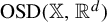 $\mathrm {OSD}(\mathbb {X},\mathbb {R}\hspace {0.5pt}^d)$
coincides with the upper box counting dimension of the metric space
 $( [\mathbb {X}^{}_{0}] , D )$
.
Proof. Let
 $\delta \in (0,\rho /2)$
and recall from Lemma 3.9 that
 $D^{}_{\hspace {-0.5pt}\delta }$
is a pseudometric on
 $\mathbb {X}^{}_{0}$
. Identifying points in
 $\mathbb {X}^{}_{0}$
with vanishing distance in the pseudometric
 $D^{}_{\hspace {-0.5pt}\delta }$
yields a quotient metric space
 $(\mathbb {X}^{\delta }_{0} , D^{}_{\hspace {-0.5pt}\delta })$
with
 $\mathbb {X}^{\delta }_{0}$
consisting of equivalence classes
 $[x]^{}_{\delta } \in \mathbb {X}^{}_{0}$
. Since
 $\nu $
-separated sets in this space are in one-to-one correspondence with
 $(\delta ,\nu )$
-separated sets in
 $\mathbb {X}^{}_{0}$
, we obtain that the upper box counting dimension of
 $(\mathbb {X}^{\delta }_{0} , D^{}_{\hspace {-0.5pt}\delta })$
can be written as
 $$ \begin{align} \limsup_{\nu {\scriptscriptstyle\searrow} 0} \frac{\log ( \mathrm{Sep\hspace{0.5pt}}(\mathbb{X}^{}_{0},\delta,\nu) )} {-\!\log(\nu)}. \end{align} $$
By Lemmas 3.11 and 3.12, the map
 $ \psi : \mathbb {X}^{\delta }_{0} \xrightarrow {\quad } [\mathbb {X}^{}_{0}]$
with
 $[x]^{}_{\delta } \mapsto [x] $
is well defined and bi-Lipshitz continuous. Hence, the upper box counting dimension of
 $([\mathbb {X}^{}_{0}],D)$
coincides with the corresponding dimension of
 $( \mathbb {X}^{\delta }_{0} , D^{}_{\hspace {-0.5pt}\delta } )$
given in equation (3.1). Up to taking a supremum over all
 $\delta \in (0,\rho /2)$
, this is precisely the expression for
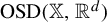 $\mathrm {OSD}(\mathbb {X},\mathbb {R}\hspace {0.5pt}^d)$
given in Corollary 3.8.
Let us now turn to the action of the inflation map on the transversal, which will provide a powerful tool for the computation of the
 $\mathrm {OSD}$
.
4 The iterated function system
In Corollary 3.5, we have seen that the inflation
 $\varrho $
maps the transversal
 $\mathbb {X}^{}_{0}$
into itself. As we shall see, this induces a map of
 $[\mathbb {X}^{}_{0}]$
into itself. Our plan is to show that an appropriate partition of
 $[\mathbb {X}^{}_{0}]$
is the fixed point of a graph-directed iterated function system. In [Reference Fuhrmann and Gröger21], a similar, but simpler construction was used for constant-length substitutions, which cannot be extended to the general tiling case.
We start by showing that the inflation indeed acts as a contraction on
 $[\mathbb {X}^{}_{0}]$
. We recall a result of Solomyak [Reference Solomyak37], who showed that the dynamical system
 $(\mathbb {X},\mathbb {R}\hspace {0.5pt}^d)$
has pure-point spectrum if and only if, for all
 $x \in \mathbb {X}$
and every return vector
 $t_{\mathrm {r}}$
, the asymptotic density of the discrepancy set
 $\mathrm {disc} ( \varrho ^{n}(x) , \varrho ^{n}(x+t_{\mathrm {r}} ))$
tends to zero as
 $n \to \infty $
, that is,
 $$ \begin{align} \lim_{n\to\infty} D ( \varrho^{n}(x), \varrho^{n}(x+t_{\mathrm{r}} ) ) = 0. \end{align} $$
Equation (4.1) can be verified via the overlap algorithm [Reference Solomyak37] or variants [Reference Akiyama, Gähler and Lee2, Reference Akiyama and Lee3, Reference Sirvent and Solomyak35] of it. An overlap in a pair of tilings x,
 $x+ t_{\mathrm {r}}$
consists of a pair of tiles, one from x and one from
 $x+ t_{\mathrm {r}}$
, such that their supports have an intersection with non-empty interior. Such an overlap is like a new kind of tile. Its support is the intersection of the supports of the two tiles and its type is a combination of the two tile types involved, together with the offset of the two tiles relative to the support of the overlap. Effectively, positioning x and
 $x+ t_{\mathrm {r}}$
on top of each other, this procedure dissects the resulting pattern into compact pieces, the overlaps.
Overlaps form equivalence classes under the translation action, thereby defining overlap types. We can define an induced inflation action on the overlaps, by inflating the two tiles of an overlap and then splitting the overlap of the two inflated tiles into tile overlaps. Solomyak has shown that, for FLC inflation tilings with an inflation factor that is a Pisot–Vijayaraghavan (PV) number, the total number of different overlap types remains bounded when r is varied and the inflation iterated. The resulting overlap inflation is denoted by
 $\varrho ^{}_{\mathrm {o}}$
and scales with the same inflation factor as
 $\varrho $
. It is no longer primitive, however.
In fact, there is a special subset of overlaps, the coincidence overlaps, which consist of pairs of tiles of the same type at the same position. These transform among themselves under inflation and form a primitive subsystem. The remaining overlaps are called discrepancy overlaps. The asymptotic density of the set covered by the discrepancy overlaps can shrink under inflation only if new coincidences are produced from discrepancy overlaps. We have the following result of Solomyak.
Theorem 4.1. [Reference Solomyak37]
The TTDS
 $(\mathbb {X},\mathbb {R}\hspace {0.5pt}^d)$
has pure-point spectrum if and only if every overlap eventually produces a coincidence overlap under the overlap inflation.
Remark 4.2. It may actually be advantageous to dissect the discrepancy region into different pieces, such as the balanced pair [Reference Sirvent and Solomyak35] discrepancies in the one-dimensional case. The advantage is that discrepancy overlaps can then be combined into natural groups, which always occur together.
Example 4.3. Let us illustrate discrepancies and overlaps with a simple example, the Fibonacci tiling [Reference Baake and Grimm11, Example 4.6]. It is generated by an inflation
 $$ \begin{align*} \varrho_{_{\mathrm{F}}} : \quad a \rightarrow ab, \quad b \rightarrow a, \end{align*} $$
where a and b are two intervals of length
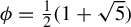 $\phi =\tfrac 12(1+\sqrt {5})$
and
 $1$
, respectively. The inflation factor is
 $\phi $
. We fist look at balanced pairs, which are (unordered) pairs of patches of tiles having the same support. A balanced pair is irreducible if the two patches have no inner vertices in common. Otherwise, it can be split into a sequence of irreducible ones at the shared inner vertices. Obviously, there are two balanced pairs which consist of a pair of equal tiles,
 $A=(a,a)$
and
 $B=(b,b)$
. These are called coincidences. If we superimpose two Fibonacci tilings in such a way that they share some of the tiles, but not all, we can decompose this bi-layer tiling into a sequence of irreducible balanced pairs. It is not difficult to see that only a small set of further balanced pairs occurs in this decomposition, namely
 $C=(ab,ba)$
and
 $D=(aab,baa)$
; compare [Reference Sirvent and Solomyak35].
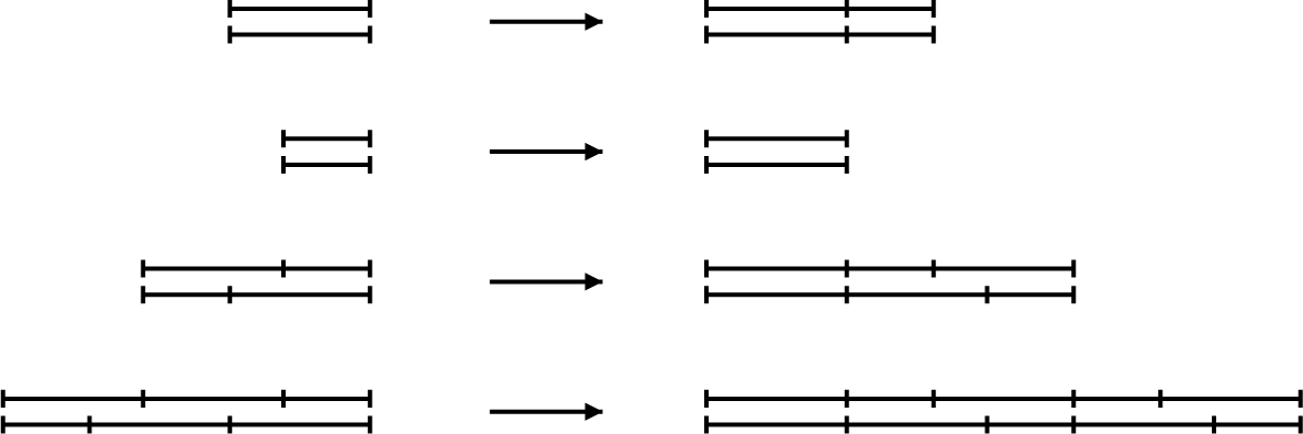
The original inflation
 $\varrho $
can be extended to balanced pairs, by inflating the two patches and then decomposing the result into irreducible balanced pairs; see Figure 1. We obtain
 $$ \begin{align*} A \rightarrow AB, \quad B \rightarrow A, \quad C \rightarrow AC, \quad D \rightarrow ACC. \end{align*} $$
We see that both discrepancies, C and D, produce a coincidence A under inflation, which proves that the Fibonacci TTDS has pure-point spectrum. Moreover, D is never produced by inflation and so the D terms are quickly eliminated under inflation and need not be considered further. Therefore, C is the only essential balanced pair discrepancy remaining.
Inflation of balanced pair overlaps A–D (from top to bottom).

Let us now decompose C into discrepancy overlaps in the above sense. The two patches in C have two interior vertices that are not shared. We cut C at those vertices into three pieces which are the three discrepancy overlaps,
 $C=C_1C_2C_3$
, as in Figure 1. Here,
 $C_1$
consists of a pair of an a tile and a b tile, which share their left vertices, resulting in an overlap region of length
 $1$
;
 $C_3$
is analogous, except that here the right vertices are shared;
 $C_2$
consists of a pair of a tiles, which are shifted by a distance
 $1$
with respect to each other, resulting in an overlap region of length
 $\phi -1$
. The coincidences A and B are also coincidence overlaps. Analogously to balanced pairs, we can extend the inflation to overlaps, giving
 $$ \begin{align*} C_1 \rightarrow A, \quad C_2 \rightarrow C_1, \quad C_3 \rightarrow C_2C_3. \end{align*} $$
We see that, after three iterations, every discrepancy overlap
 $C_i$
has produced at least one coincidence, which proves again the pure-point nature of the Fibonacci tiling spectrum.
Since we assume a system with topological pure-point spectrum, Theorem 4.1 implies that some fixed power of the overlap inflation produces a coincidence from every overlap. This can now be used to prove the following result.
Proposition 4.4. Assume that the TTDS
 $(\mathbb {X},\mathbb {R}\hspace {0.5pt}^d)$
has topological pure-point spectrum. Then, there exist numbers
 $n \in \mathbb {N}$
and
 $r^{}_{\hspace {-0.5pt}\mathrm {c}} \in (0, 1)$
, such that, for all
 $x,y \in \mathbb {X}^{}_{0}$
,
 $$ \begin{align*} D ( \varrho^n(x),\varrho^n(y)) \leqslant r^{}_{\hspace{-0.5pt}\mathrm{c}}D(x,y). \end{align*} $$
Proof. We first note that, by the construction of our control points, there exists a power
 $\varrho ^{k_1}$
of the inflation such that, for any
 $x,y\in \mathbb {X}^{}_{0}$
, the tilings
 $\varrho ^{k_1}(x)$
and
 $\varrho ^{k_1}(y)$
have some coincidences. Starting from such a pair, by Theorem 4.1, there exists a power
 $\varrho ^{k_2}$
that produces a coincidence from every overlap. Hence, there exists
 $r^{}_{\hspace {-0.5pt}\mathrm {c}} <1$
such that
 $$ \begin{align*} D ( \varrho^{k_1+k_2}(x),\varrho^{k_1+k_2}(y) ) \leqslant r^{}_{\hspace{-0.5pt}\mathrm{c}} \hspace{0.5pt} D ( \varrho^{k_1}(x),\varrho^{k_1}(y) ) \leqslant r^{}_{\hspace{-0.5pt}\mathrm{c}} \hspace{0.5pt} D(x,y). \end{align*} $$
Consequently,
 $\varrho ^{k_1+k_2}$
is a contraction on
 $\mathbb {X}^{}_{0}$
with contraction constant
 $r^{}_{\hspace {-0.5pt}\mathrm {c}}$
relative to the pseudometric D.
As all powers of
 $\varrho $
generate the same hull, we may assume
 $D(\varrho (x),\varrho (y)) \leqslant r^{}_{\hspace {-0.5pt}\mathrm {c}} \hspace {0.5pt} D(x,y)$
from now on. We are now ready to construct appropriately defined components of
 $[\mathbb {X}^{}_{0}]$
as the unique fixed point of a (graph-directed) iterated function system (GIFS). For this purpose, we partition
 $\mathbb {X}^{}_{0}$
into cylinder sets
 $\mathbb {X}_i$
. Labelling tile types with natural numbers
 $i \in \{ 1,2,\ldots , n_{\tau } \}$
, the cylinder
 $\mathbb {X}_i$
consists of all tilings in
 $\mathbb {X}^{}_{0}$
that have a tile of type i with its control point at the origin. Due to the recognizability property of aperiodic inflation tilings, the tile at the origin of any tiling in
 $\mathbb {X}_i$
is contained in a unique supertile, which must be positioned so that it has a tile of type i at the origin. Hence,
 $\mathbb {X}_i$
is a disjoint union of smaller cylinder sets,
 $$ \begin{align} \mathbb{X}_i = \bigcup_j\bigcup_k (\varrho(\mathbb{X}_j) - t_{ij;k} ) , \end{align} $$
where j runs over all supertile types which contain a tile of type i, and the
 $t_{ij;k}$
are the positions of such a tile within the supertile.
Applying the projection to the MEF on both sides of equation (4.2) (and using that
 $\varrho $
commutes with this factor map) yields a similar relation with
 $\mathbb {X}_i$
replaced by
 $[\mathbb {X}_i]$
for all i. In contrast to the approach of [Reference Fuhrmann and Gröger21], the unions will no longer be completely disjoint, as there may be fibres which are split over several cylinders. These overlaps will be small, however. Let us now translate equation (4.2) (with
 $\mathbb {X}_i$
replaced by
 $[\mathbb {X}_i]$
) into the language of a GIFS; see [Reference Edgar and Golds19].
Definition 4.1. We call
 $\{ \mathcal {G}, \{(X_i,d_i)\}_{i \in V}, \{f_e \}_{e \in E} \}$
a GIFS if
 $\mathcal {G}$
is a graph with vertex set V and edge set E, each
 $(X_i,d_i)$
is a compact metric space, and for each
 $e \in E_{ij}$
, the set of edges from i to j, the map
 $f_e: X_j \to X_i$
is a strict contraction. A tuple
 $\{Y_i \}_{i \in V}$
of compact sets
 $Y_i \subseteq X_i$
is called an invariant list of the GIFS if
 $ Y_i = \bigcup _{j \in V} \bigcup _{e \in E_{ij}} f_e(Y_j)$
for all
 $i \in V$
.
Here, we let V be the set of tile types and may choose
 $(X_i,d_i) = ( [\mathbb {X}_i], D )$
for the metric spaces. Note that each
 $[\mathbb {X}_i]$
is compact as the image of a compact set under a continuous map. There is an edge e for each occurrence of a tile of type i in a supertile of type j, indexed by k. If
 $t_{ij;k}$
is the corresponding position in the supertile, we set
 $f_e ( [x] ) \mathrel {\mathop :}= \varrho ( [x] ) - t_{ij;k}$
. Since the metric D is translation invariant, we conclude from Proposition 4.4 that the maps
 $f_e$
are indeed all strict contractions. With this notation, the projection of equation (4.2) to the MEF yields
 $$ \begin{align} [\mathbb{X}_i] = \bigcup_{j\in V}\bigcup_{e\in E_{ij}} f_e ( [\mathbb{X}_j] ). \end{align} $$
That is,
 $\{ [\mathbb {X}_i] \}_{i \in V}$
is an invariant list of this GIFS and the
 $\mathrm {OSD}$
is nothing but the (upper) box dimension of
 $[\mathbb {X}^{}_{0}] = \bigcup _{i \in V} [\mathbb {X}_i]$
relative to D. If
 $\mathcal {G}$
is strongly connected, which is the case for primitive inflation tilings, the invariant list is in fact unique. We note that the fractal dimension of the fixed point space
 $\{ [\mathbb {X}_i] \}_{i \in V}$
, relative to D, can be estimated from the graph
 $\mathcal {G}$
and the contraction rates of the maps
 $f_e$
. This is a classic result if each
 $f_e$
is a similarity on a Euclidean space. A version for more general contractions on metric spaces, involving upper and lower bounds on the contraction rates, can be found in [Reference Edgar and Golds19]. We recall it here for the sake of being self-contained. To obtain a lower bound, we require an appropriate separation condition.
Definition 4.2. We say that the GIFS
 $( \mathcal {G}, \{X_i \}^{}_{i \in V}, \{f_e \}^{}_{e \in E} )$
with invariant list
 $\{ Y_i \}^{}_{i \in V}$
satisfies the strong open set condition (SOSC) if there is a collection of open sets
 $\{U_i \}^{}_{i \in V}$
with the following properties.
-
(1) For all
$i,j \in V$
,
$e \in E_{ij}$
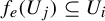
, we have
$f_e(U_j)\subseteq U_i$
. -
(2) For all
$i,j,j' \in V$
,
$e\in E_{ij}$
,
$e'\in E_{ij'}$
,
$e \ne e'$
, we have
$f_e(U_j) \cap f_{e'}(U_{j'}) = \varnothing $
. -
(3) For all
$i \in V$
, we have
$U_i \cap Y_i \ne \varnothing $
.







The following is a special case (uniform bounds on all contractions) of a slightly more general result in [Reference Edgar and Golds19]. To formulate the result, let M denote the incidence matrix of the graph
 $\mathcal {G}$
, with entries
 $M_{ij} = \operatorname {{\mathrm {card}}} ( E_{ij} )$
, and
 $\rho ^{}_{\mathrm {sp}}(M)$
the corresponding spectral radius.
Theorem 4.5. [Reference Edgar and Golds19]
Let
 $( \mathcal {G}, \{X_i \}^{}_{i \in V}, \{f_e \}^{}_{e \in E} )$
be a GIFS with invariant list
 $\{ Y_i \}^{}_{i \in V}$
and let
 $\mathcal {G}$
be strongly connected. Assume that the GIFS satisfies the SOSC and let
 $\dim $
denote Hausdorff dimension, lower box counting dimension or upper box counting dimension. If there are numbers
 $0 < r^{}_{\hspace {-0.5pt}\mathrm {c}} \leqslant r^{\hspace {0.5pt}\prime }_{\hspace {-0.5pt}\mathrm {c}} <1$
with
 $$ \begin{align*} r^{}_{\hspace{-0.5pt}\mathrm{c}} \hspace{0.5pt} d^{}_j(x,y) \leqslant d^{}_i ( f^{}_e(x) , f^{}_e (y) ) \leqslant r^{\hspace{0.5pt}\prime}_{\hspace{-0.5pt}\mathrm{c}} \hspace{0.5pt} d^{}_j(x,y) \end{align*} $$
for all
 $e \in E_{ij}$
,
 $i,j \in V$
and
 $x,y \in X_j$
, then, for all
 $i \in V$
, we have that
 $$ \begin{align*} \frac{\log (\rho^{}_{\mathrm{sp}}(M))} {-\! \log(r^{}_{\hspace{-0.5pt}\mathrm{c}})} \leqslant \dim ( Y^{}_i ) \leqslant \frac{\log (\rho^{}_{\mathrm{sp}}(M))} {-\! \log(r^{\hspace{0.5pt}\prime}_{\hspace{-0.5pt}\mathrm{c}})}. \end{align*} $$
In view of this result, we naturally strive to verify the SOSC for the GIFS at hand. For this purpose, we define sets
 $U_j = \{[x] \in [\mathbb {X}_j]: [x] \subset \mathbb {X}_j \}$
, consisting of fibres which are completely contained in a single cylinder. Since generic fibres contain a single element [Reference Aujogue, Barge, Kellendonk, Lenz, Kellendonk, Lenz and Savinien5], the sets
 $U_j$
are all non-empty. Let us point out that an equivalence class
 $[x] \in [\mathbb {X}_j]$
always intersects
 $\mathbb {X}_j$
, but may also contain points from
 $\mathbb {X}\setminus \mathbb {X}_j$
. However, since we are dealing with repetitive Meyer sets, it is known that there are only finitely many possible positions for the closest control point of type j to the origin in y if
 $y \sim x \in \mathbb {X}_j$
; compare [Reference Aujogue, Barge, Kellendonk, Lenz, Kellendonk, Lenz and Savinien5, Corollary 4.17]. In a slightly different formulation, this yields the following result.
Lemma 4.6. Given
 $(\mathbb {X},\mathbb {R}\hspace {0.5pt}^d)$
as above, there is a characteristic constant
 $\kappa> 0$
with the following property. If
 $y \sim x \in \mathbb {X}_j$
and
 $y \notin \mathbb {X}_j$
, then
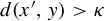 $d(x',y)> \kappa $
for all
 $x'\in \mathbb {X}_j$
.
This dichotomy is useful for the proof of the following observation.
Lemma 4.7. For each j, the set
 $U_j = \{ [x] \in [\mathbb {X}_j]: [x] \subseteq \mathbb {X}_j \}$
is open in
 $[\mathbb {X}_j]$
.
Proof. Assume the contrary. Then, there exists a point
 $[x]\in U_j$
such that every open neighbourhood of
 $[x]$
contains a point in
 $[\mathbb {X}_j] \setminus U_j$
. That is, we can find a sequence of points
 $[x_n] \in [\mathbb {X}_j] \setminus U_j$
such that
 $[x_n] \to [x]$
as
 $n \to \infty $
. By the definition of
 $U_j$
and
 $[\mathbb {X}_j]$
, every equivalence class
 $[x_n]$
has a representative
 $x_n \notin \mathbb {X}_j$
and a representative
 $x^{\hspace {0.5pt}\prime }_n \in \mathbb {X}_j$
with
 $x^{}_n \sim x^{\hspace {0.5pt}\prime }_n$
. By Lemma 4.6, the distance of
 $x_n$
to
 $\mathbb {X}_j$
is bounded away from zero. This shows that the limit point
 $x^{\hspace {0.5pt}\prime }$
of an arbitrary converging subsequence
 $(x_{n_j})$
is not contained in
 $\mathbb {X}_j$
. However, due to the continuity of the factor map,
 $$ \begin{align*}[x{\hspace{0.5pt}}'] = \Big[\kern-2pt\lim_{j \to \infty} x_{n_j} \kern-2pt\Big] = \lim_{j \to \infty} [x_{n_j}] = [x]. \end{align*} $$
Consequently, the fibre
 $[x] \in U_j$
contains an element
 $x{\hspace {0.5pt}}'$
in the complement of
 $\mathbb {X}_j$
, in contradiction to the definition of
 $U_j$
.
Proposition 4.8. Assume again that we have a non-periodic tiling dynamical system with pure-point spectrum, which is generated by a primitive inflation rule. Then, the corresponding GIFS satisfies the SOSC, with open sets
 $U_j$
as defined above.
Proof. Since
 $U_j \subseteq [\mathbb {X}_j]$
is non-empty, the third condition is immediate. Let
 $e \in E_{ij}$
and
 $[x] \in U_j$
. Then, all points in the equivalence class
 $f_e ( [x] )$
are contained in
 $f_e(\mathbb {X}_j)$
. Indeed, using equation (2.3) in the first step, we obtain
 $$ \begin{align*} f_e ( [x] ) = \{ f_e(x') : x'\in [x] \} \subseteq f_e (\mathbb{X}_j), \end{align*} $$
because
 $[x] \in U_j, \text{and hence } [x] \subseteq \mathbb {X}_j$
. Since
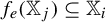 $f_e(\mathbb {X}_j) \subseteq \mathbb {X}_i$
, it follows that each element of the fibre
 $f_e ( [x] )$
is also contained in
 $\mathbb {X}_i$
, which shows that
 $f_e ( [x] ) \in U_i$
. That is,
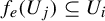 ${f_e(U_j) \subseteq U_i}$
, as required for the first condition. Finally, if
 $e \in E_{ij'}$
and
 $[x{\hspace {0.5pt}}'] \in U_{j'}$
, we see by identical arguments as before that the fibre
 $f_{e'} ( [x'] )$
is contained in
 $f_{e'}(\mathbb {X}_{j'})$
. By recognizability of the inflation, this set is disjoint from
 $f_e(\mathbb {X}_j)$
. Hence, the fibres
 $f_{e} ( [x] )$
and
 $f_{e'} ( [x{\hspace {0.5pt}}'] )$
have no point in common, that is,
 $f_{e} ( [x] ) \neq f_{e'} ( [x{\hspace {0.5pt}}'] )$
for all
 $[x] \in U_j$
and
 $[x{\hspace {0.5pt}}'] \in U_{j'}$
. This is precisely what is required for the second condition.
At this point, we have established that Theorem 4.5 can indeed be applied to the invariant list
 $\{ [\mathbb {X}_i] \}_{i \in V}$
. This gives bounds for the upper box counting dimension of
 $( [\mathbb {X}^{}_{0}], D )$
, where the latter coincides with the
 $\mathrm {OSD}$
by Theorem 3.13. The precise values of the bounds depend on estimates for the contraction rates of the maps
 $f_e$
, which are the same as the corresponding estimates for
 $\varrho $
. As passing to higher powers of
 $\varrho $
might yield better bounds, this motivates the following definition.
Definition 4.3. For each
 $n \in \mathbb {N}$
, let
 $r_n,R_n \geqslant 0$
be such that
 $$ \begin{align*} r_n D(x,y) \leqslant D ( \varrho^n(x), \varrho^n(y) ) \leqslant R_n D(x,y) \end{align*} $$
for all
 $x,y \in \mathbb {X}_i$
and
 $i \in V$
, and assume that
 $r_n$
is maximal (
 $R_n$
is minimal) with this property.
We are interested in the decay properties of these contraction bounds as
 $n \to \infty $
.
Lemma 4.9. The sequence
 $(R_n)^{}_{n \in \mathbb {N}}$
is sub-multiplicative, while the sequence
 $(r_n)^{}_{n \in \mathbb {N}}$
is super-multiplicative. In particular, the Lyapunov exponents

are well defined.
Proof. For
 $n,m \in \mathbb {N}$
, the estimate
 $D(\varrho ^{n+m}(x),\varrho ^{n+m}(y)) \leqslant R_n R_m D(x,y)$
follows from the definition. Since the same bound holds with
 $R_n R_m$
replaced by
 $R_{n+m}$
, and the latter is minimal with this property, we conclude that
 $R_{n+m} \leqslant R_n R_m$
. The estimate
 $r_{n+m} \geqslant r_n r_m$
follows analogously. The remaining statements are consequences of Fekete’s lemma.
Let us remark that, in the present setup, the incidence matrix of the GIFS coincides with the inflation matrix M of
 $\varrho $
, where
 $M_{ij}$
is the number of occurrences of a tile of type i in a supertile of type j. Since the inflation factor
 $\unicode{x3bb} $
means that volumes in
 $\mathbb {R}\hspace {0.5pt}^d$
scale with
 $\unicode{x3bb} ^d$
under the action of
 $\varrho $
, we get
 $\unicode{x3bb} ^d$
as the leading eigenvalue of M.
Theorem 4.10. For a self-similar and non-periodic TTDS
 $(\mathbb {X},\mathbb {R}\hspace {0.5pt}^d)$
with pure-point spectrum, generated by a primitive inflation
 $\varrho $
with inflation factor
 $\unicode{x3bb} $
, the
 $\mathrm {OSD}$
satisfies the bounds

where
 $\unicode{x3bb} _{\mathrm {L}}^{\mathrm \min }$
and
 $\unicode{x3bb} _{\mathrm {L}}^{\mathrm \max }$
are the minimal and maximal Lyapunov exponents, respectively.
Proof. By Theorem 3.13, the
 $\mathrm {OSD}$
is given by the upper box counting dimension of the metric space
 $( [\mathbb {X}^{}_{0}] , D )$
, and since
 $[\mathbb {X}^{}_{0}] = \bigcup _{i \in V} [\mathbb {X}_i]$
, this coincides with the maximal dimension of
 $[\mathbb {X}_i]$
, with
 $i \in V$
. The list
 $\{[\mathbb {X}_i]\}_{i \in V}$
is invariant under a (strongly connected) GIFS that satisfies the SOSC, due to Proposition 4.8. Hence, applying Theorem 4.5 to the GIFS induced by the inflation
 $\varrho ^n$
, we obtain
 $$ \begin{align} \frac{n \log (\rho^{}_{\mathrm{sp}}(M))}{-\!\log(r_n)} \leqslant \: \overline{\dim}^{}_B ( [\mathbb{X}_i] ) \leqslant \frac{n \log (\rho^{}_{\mathrm{sp}}(M))}{-\!\log(R_n)} \end{align} $$
for each
 $n \in \mathbb {N}$
and
 $i \in V$
, where
 $\overline {\dim }^{}_B$
denotes the upper box counting dimension. Since M is primitive with leading eigenvalue
 $\unicode{x3bb} ^d$
, we have
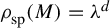 $\rho ^{}_{\mathrm {sp}}(M)=\unicode{x3bb} ^d$
. Performing the limit
 $n \to \infty $
on both bounds in equation (4.4) yields the assertion.
As discussed earlier in this section, the contraction rates needed for these bounds are governed by the overlap inflation
 $\varrho ^{}_{\mathrm {o}}$
, or more precisely, by the part of
 $\varrho ^{}_{\mathrm {o}}$
that acts on the discrepancy overlaps. Let us call this part the discrepancy inflation
 $\varrho ^{}_{\mathrm {dc}}$
and denote its inflation matrix by
 $M_{\mathrm {dc}}$
. The substitution
 $\varrho ^{}_{\mathrm {dc}}$
produces discrepancies from discrepancies, omitting any coincidences that would be produced by
 $\varrho ^{}_{\mathrm {o}}$
. Due to this omission, the leading eigenvalue
 $\unicode{x3bb} ^{}_{\mathrm {dc}} = \rho ^{}_{\mathrm {sp}}(M_{\mathrm {dc}})$
must be smaller than the leading eigenvalue
 $\unicode{x3bb} ^d$
of
 $\varrho ^{}_{\mathrm {o}}$
.
Let us now consider, for each discrepancy type i, the smallest set
 $S_i$
of overlap types that is invariant under
 $\varrho ^{}_{\mathrm {dc}}$
and includes i. Let
 $\unicode{x3bb} _i$
be the leading eigenvalue of
 $\varrho ^{}_{\mathrm {dc}}$
, confined to the invariant subset
 $S_i$
of discrepancy types. Given an overlap of type i, its geometric image grows with the inflation factor
 $\unicode{x3bb} ^d$
under the substitution
 $\varrho $
, whereas the total amount covered by overlaps scales (eventually) with
 $\unicode{x3bb} _i$
. This yields the following result.
Proposition 4.11. Under the general assumptions of Theorem 4.10, we have

Proof. For
 $j \in V$
and
 $x,y \in \mathbb {X}_j$
with
 $x \not \sim y$
, let
 $v = v(x,y)$
be a vector containing the relative frequencies of discrepancy types (normalized to
 $\| v \|^{}_1 = 1$
). Then, the ratio
 $D( \varrho ^n(x),\varrho ^n(y))/D(x,y)$
is given by
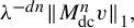 $ \unicode{x3bb} ^{-dn} \| M_{\mathrm {dc}}^{n} v \|^{}_1, $
up to a multiplicative constant that is independent of
 $n \in \mathbb {N}$
and the choices of
 $x,y$
(accounting for the varying volumes of different discrepancy types). Due to the non-negativity of both v and
 $M_{\mathrm {dc}}$
, we observe that
 $\| M_{\mathrm {dc}}^{n} v \|^{}_1$
can be written as a convex combination of the values
 $\| M_{\mathrm {dc}}^{n} e^{}_i \|^{}_1$
, where
 $e_i$
denotes the Euclidean unit vector corresponding to type i. In particular,
 $$ \begin{align*} \min_i \unicode{x3bb}^{-dn} \| M^n_{\mathrm{dc}} e^{}_i \|^{}_1 \leqslant \unicode{x3bb}^{-dn} \| M^n_{\mathrm{dc}} v \|^{}_1 \leqslant \max_i \unicode{x3bb}^{-dn} \| M^n_{\mathrm{dc}} e^{}_i \|^{}_1. \end{align*} $$
By definition, these bounds (up to a constant) also hold for
 $r_n$
and
 $R_n$
. Since
 $\unicode{x3bb} _i$
coincides with the growth rate of
 $\| M_{\mathrm {dc}}^n e^{}_i \|^{}_1$
, this implies

Given a discrepancy of type i, let
 $x \in \mathbb {X}^{}_{0}$
and t be such that i appears in the overlap decomposition of x and
 $x+t$
. This implies that there is a pattern P in x such that the intersection of P and
 $P+t$
contains an overlap of type i. Since x is repetitive, this pattern appears with positive frequency and we conclude that type i actually occurs with positive frequency in the pair
 $( x,x+t )$
. Choosing i such that
 $\unicode{x3bb} _i = \unicode{x3bb} _{\mathrm {dc}}$
is maximal, we obtain that there is in fact a pair
 $(x,x+t)$
such that
 $D(\varrho ^n(x),\varrho ^n(x+t))$
decays with the slowest possible contraction rate. That is, we have
 $\unicode{x3bb} _{\mathrm {L}}^{\max } = \log (\unicode{x3bb} _{\mathrm {dc}}) - d\hspace {0.5pt} \log (\unicode{x3bb} )$
.
Corollary 4.12. If
 $\varrho ^{}_{\mathrm {dc}}$
is primitive or if every invariant subsystem
 $S_i$
contains a leading eigenvalue
 $\unicode{x3bb} _{\mathrm {dc}}$
, then

and hence

Remark 4.13. We should emphasize again that there are two inflations involved, the inflation
 $\varrho $
acting on
 $[\mathbb {X}^{}_{0}]$
, and the discrepancy inflation
 $\varrho ^{}_{\mathrm {dc}}$
, which determines the contraction rates of
 $\varrho $
. To obtain these contraction rates, we only needed the combinatorial properties of
 $\varrho ^{}_{\mathrm {dc}}$
, but not a geometric realization. If the overlap algorithm is used to determine pure-pointedness, these combinatorial properties can be obtained as a byproduct.
Remark 4.14. There are examples where the balanced pair discrepancy inflation is primitive, whereas the overlap discrepancy inflation is not. Using the latter, one would have to show that the fast-shrinking discrepancies in an invariant subsystem
 $S_i$
always occur together with other slower-shrinking discrepancies.
5 Product tilings
The simplest way to obtain higher-dimensional tilings is to build direct products of lower-dimensional ones. Let us assume we have two dynamical systems
 $(\mathbb {X},\mathbb {R}^{d_{\mathbb {X}}})$
and
 $(\mathbb {Y},\mathbb {R}^{d_{\mathbb {Y}}})$
, each with well-defined
 $\mathrm {OSD}$
. We are then interested in the
 $\mathrm {OSD}$
of the product system
 $(\mathbb {X} \times \mathbb {Y}, \mathbb {R}^{d_{\mathbb {X}}+d_{\mathbb {Y}}})$
. We equip the product space
 $\mathbb {X} \times \mathbb {Y}$
with the sup metric of the individual metrics. In the case of tiling spaces, this is not the same as the natural tiling metric on
 $\mathbb {X} \times \mathbb {Y}$
as defined in §2, but is equivalent to it and thus does not affect the
 $\mathrm {OSD}$
. Also, we naturally compute the
 $\mathrm {OSD}$
with respect to the product of the two Følner sequences that are used for the individual dynamical systems. Product systems had already been considered in [Reference Fuhrmann, Gröger and Jäger22, Reference Fuhrmann, Gröger, Jäger and Kwietniak23], though with equal groups acting on the factors and with the diagonal action on the product. As we shall see, this difference is not essential for our purpose.
Let us first observe that the
 $\mathrm {OSD}$
can equivalently be defined with spanning instead of separation numbers, as already noted in [Reference Fuhrmann, Gröger, Jäger and Kwietniak23]. We specify the
 $(\delta ,\nu )$
-span of a set
 $S\subset \mathbb {X}$
as
 $$ \begin{align*} \{x\in\mathbb{X}: \text{ there exists } y \in S \text{ with } D^{}_{\hspace{-0.5pt}\delta}(x,y)\leqslant \nu \}, \end{align*} $$
and we say that S is
 $(\delta ,\nu )$
-spanning if its
 $(\delta ,\nu )$
-span is the entire space
 $\mathbb {X}$
. We then set the spanning number
 $\textrm {Span}(\mathbb {X},\delta ,\nu )$
to be the minimal cardinality of a
 $(\delta ,\nu )$
-spanning subset
 $S\subseteq \mathbb {X}$
. The following result was shown for
 $\mathbb {Z}\hspace {0.5pt}$
-actions in [Reference Fuhrmann, Gröger and Jäger22], but the proof carries over verbatim to the case of more general group actions; compare also the discussion in [Reference Fuhrmann, Gröger, Jäger and Kwietniak23].
Lemma 5.1. The separation numbers and spanning numbers satisfy the relations
 $$ \begin{align*} \mathrm{Span}\hspace{0.5pt}(\mathbb{X},\delta,\nu) \leqslant \mathrm{Sep\hspace{0.5pt}}(\mathbb{X},\delta,\nu) \leqslant \mathrm{Span}\hspace{0.5pt}(\mathbb{X}, \delta/2,\nu/2). \end{align*} $$
This lemma shows that the
 $\mathrm {OSD}$
is unchanged by replacing the separation numbers in its definition by the spanning numbers. Given two product tilings
 $x^{}_1 \hspace {-0.5pt}\times y^{}_1$
and
 $x^{}_2 \times y^{}_2$
, with
 $x^{}_i \in \mathbb {X}$
and
 $y^{}_i \in \mathbb {Y}$
, the definition of the sup metric implies that
 $$ \begin{align*} \varDelta^{}_{\delta} (x^{}_1 \times y^{}_1, x^{}_2 \times y^{}_2) = ( \varDelta^{}_{\delta} (x^{}_1, x^{}_2) \times \mathbb{R}\hspace{0.5pt}^{d_{\mathbb{Y}}}) \cup ( \mathbb{R}\hspace{0.5pt}^{d_{\mathbb{X}}}\hspace{-0.5pt} \times\hspace{-0.5pt} \varDelta^{}_{\delta} (y^{}_1 , y^{}_2) ). \end{align*} $$
Taking upper densities on both sides gives
 $$ \begin{align} \max \{ D^{}_{\hspace{-0.5pt}\delta} (x^{}_1 , x^{}_2), D^{}_{\hspace{-0.5pt}\delta} (y^{}_1 , y^{}_2) \} \leqslant D^{}_{\hspace{-0.5pt}\delta} ( x^{}_1 \hspace{-0.5pt} {\times\hspace{0.5pt}} y^{}_1, x^{}_2 {\hspace{0.5pt}\times\hspace{0.5pt}} y^{}_2 ) \leqslant D^{}_{\hspace{-0.5pt}\delta} (x^{}_1 , x^{}_2) + D^{}_{\hspace{-0.5pt}\delta} (y^{}_1 , y^{}_2 ). \end{align} $$
This leads to the following analogue of the product rules derived in [Reference Fuhrmann, Gröger and Jäger22, Proposition 1.3].
Theorem 5.2. Let
 $(\mathbb {X} {\hspace {0.5pt}\times } \mathbb {Y}, \mathbb {R}\hspace {0.5pt}^{d_{\mathbb {X}}+d_{\mathbb {Y}}})$
be a direct product dynamical system. Assume that both factors have a well-defined, finite
 $\mathrm {OSD}$
and that the limit in equation (1.3) of the
 $\mathrm {OSD}$
exists. Then, the
 $\mathrm {OSD}$
of the product system is
 $$ \begin{align*} \mathrm{OSD}( \mathbb{X} \hspace{0.5pt}{\hspace{0.5pt}\times}\hspace{0.5pt} \mathbb{Y}, \mathbb{R}\hspace{0.5pt}^{d_{\mathbb{X}}} {\times\hspace{0.5pt}} \mathbb{R}\hspace{0.5pt}^{d_{\mathbb{Y}}} ) = \mathrm{OSD}(\mathbb{X},\mathbb{R}\hspace{0.5pt}^{d_{\mathbb{X}}}) + \mathrm{OSD}( \mathbb{Y}, \mathbb{R}\hspace{0.5pt}^{d_{\mathbb{Y}}}). \end{align*} $$
Proof. We will construct suitable separated sets and spanning sets for
 $\mathbb {X} {\hspace {0.5pt}\times } \mathbb {Y}$
. Suppose
 $S^{}_1$
and
 $S^{}_2$
are
 $(\delta ,\nu )$
-separated subsets of
 $\mathbb {X}$
and
 $\mathbb {Y}$
, respectively. By equation (5.1), the product set
 $S^{}_1 {\times \hspace {0.5pt}} S^{}_2$
is then
 $(\delta ,\nu )$
-separated in
 $\mathbb {X} {\hspace {0.5pt}\times \hspace {0.5pt}} \mathbb {Y}$
, and hence
 $$ \begin{align*} \mathrm{Sep\hspace{0.5pt}}(\mathbb{X}{\hspace{0.5pt}\times}\hspace{0.5pt}\mathbb{Y},\delta,\nu) \geqslant \mathrm{Sep\hspace{0.5pt}}(\mathbb{X},\delta,\nu) \hspace{-0.5pt}\cdot \mathrm{Sep\hspace{0.5pt}}(\mathbb{Y},\delta,\nu). \end{align*} $$
Conversely, let
 $S^{\hspace {0.5pt}\prime }_1$
and
 $S^{\hspace {0.5pt}\prime }_2$
be
 $(\delta ,\nu /2)$
-spanning subsets of
 $\mathbb {X}$
and
 $\mathbb {Y}$
, respectively. By equation (5.1),
 $S^{\hspace {0.5pt}\prime }_1 {\hspace {0.5pt}\times \hspace {0.5pt}} S^{\hspace {0.5pt}\prime }_2$
then is
 $(\delta ,\nu )$
-spanning in
 $\mathbb {X} {\hspace {0.5pt}\times } \mathbb {Y}$
, and hence
 $$ \begin{align*} \mathrm{Span}\hspace{0.5pt}(\mathbb{X}{\hspace{0.5pt}\times}\mathbb{Y},\delta,\nu) \leqslant \mathrm{Span}\hspace{0.5pt}(\mathbb{X},\delta,\nu/2) \hspace{-0.5pt}\cdot \mathrm{Span}\hspace{0.5pt}(\mathbb{Y},\delta,\nu/2). \end{align*} $$
These two inequalities, together with Lemma 5.1, prove the claim.
Remark 5.3. In the context of tiling dynamical systems generated by a primitive inflation rule, the requirement about the existence of the limit in equation (1.3) can be replaced by the corresponding condition on the transversal. This can be translated to the requirement that the upper and lower box counting dimensions of
 $( [\mathbb {X}^{}_{0},D] )$
coincide. The upper and lower bounds established via the GIFS approach hold for both kinds of dimensions. Therefore, as soon as these bounds agree, the condition is satisfied. This applies in particular to the situation in Corollary 4.12, where a closed form expression for the
 $\mathrm {OSD}$
is available.
6 Window boundaries
It is well known that primitive inflation tilings with pure-point spectrum are also cut-and-project tilings, in the sense that the control point sets are regular model sets [Reference Baake and Grimm11]. In the case of inflation tilings, however, we have to distinguish between control points belonging to different tile types, each of which will have its own window,
 $W_i$
.
It had been observed [Reference Feng, Furukado, Ito and Wu20, Reference Sing34] that the boundaries of the windows
 $W_i$
for the different tile types form the fixed point of a boundary inflation
 $\varrho ^{}_{\mathrm {bd}}$
, a GIFS that is combinatorially isomorphic to the (transposed) discrepancy inflation
 $\varrho ^{}_{\mathrm {dc}}$
. If we denote, in slight abuse of notation, by
 $\overline {\dim }_B(\partial W)$
the maximum of the upper box dimensions
 $\overline {\dim }_B(\partial W_i)$
, we thus obtain, in analogy to equation (4.4), an upper bound
 $$ \begin{align} \overline{\dim}_B(\partial W) \leqslant \frac{\log (\rho^{}_{\mathrm{sp}}(M_{\mathrm{bd}}))} {-\!\log(r^{}_{\hspace{-0.5pt}\mathrm{c}})}, \end{align} $$
where
 $\rho ^{}_{\mathrm {sp}}(M_{\mathrm {bd}})=\unicode{x3bb} _{\mathrm {dc}}$
is the leading eigenvalue of the inflation matrix
 $M_{\mathrm {bd}}$
for the boundary inflation
 $\varrho ^{}_{\mathrm {bd}}$
and
 $r^{}_{\hspace {-0.5pt}\mathrm {c}}$
is the slowest contraction rate of the inflation in internal space.
Conversely, [Reference Fuhrmann, Gröger, Jäger and Kwietniak23, Theorem 1.4] gives an upper bound on the
 $\mathrm {OSD}$
in terms of
 $\overline {\dim }_B(\partial W)$
,
 $$ \begin{align} \mathrm{OSD}(\mathbb{X},\mathbb{R}\hspace{0.5pt}^d) \leqslant \frac{d^{}_{\mathrm{int}}} {d^{}_{\mathrm{int}} \hspace{-0.5pt} - \hspace{0.5pt} \overline{\dim}_B(\partial W)}, \end{align} $$
where
 $d^{}_{\mathrm {int}}$
is the upper box dimension of internal space. Assuming that the
 $\mathrm {OSD}$
exists, this can be converted into a lower bound
 $$ \begin{align} \overline{\dim}_B(\partial W) \geqslant d^{}_{\mathrm{int}} \cdot \frac{ \mathrm{OSD}(\mathbb{X},\mathbb{R}\hspace{0.5pt}^d) - 1 }{ \mathrm{OSD}(\mathbb{X},\mathbb{R}\hspace{0.5pt}^d)}. \end{align} $$
Below, we only consider the case of a Euclidean internal space, which occurs if the inflation factor
 $\unicode{x3bb} $
is a unit. Assume further that the contraction in internal space is isotropic, which is the case when
 $\unicode{x3bb} $
is quadratic (so
 $r^{}_{\hspace {-0.5pt}\mathrm {c}}=\unicode{x3bb} ^{-1}$
) or when
 $\unicode{x3bb} $
is ternary with a complex conjugate pair of Galois conjugates (hence,
 $r^{}_{\hspace {-0.5pt}\mathrm {c}}=\unicode{x3bb} ^{-\frac 12}$
). Then, the upper bound simplifies to

where the dimension
 $d^{}_{\mathrm {int}}$
of internal space is either d or
 $2d$
. With this and the lower bound in equation (6.3), one can show the following result.
Proposition 6.1. Assume that a primitive inflation tiling with pure-point spectrum has a Euclidean internal space with isotropic contraction under the inflation and that the discrepancy inflation
 $\varrho ^{}_{\mathrm {dc}}$
is primitive (or that every invariant subsystem has the same leading eigenvalue). Then, the Hausdorff dimension of the window boundary satisfies

where
 $d_{\mathrm {int}}$
is the dimension of internal space.
Proof. The upper bound on the window boundary dimension is given by equation (6.4). The corresponding lower bound follows by combining equation (6.3) with Corollary 4.12, which yields

Again using the expression for the
 $\mathrm {OSD}$
from Corollary 4.12, a straight-forward calculation yields the claimed relation between the
 $\mathrm {OSD}$
and the window boundary dimension.
Remark 6.2. Instead of using the lower bound in equation (6.3), we can also use the lower bound of an analogue of Theorem 4.10, provided we can replace the SOSC by some other sufficient separation condition satisfied by the boundary inflation. For the case at hand, the weak separation property (WSP) (see [Reference Das and Edgar18]) can be shown to hold and is particularly simple to check. In the context of a GIFS, its sufficiency was proved by Das and Edgar [Reference Das and Edgar18]. Note, however, that also the WSP crucially depends on the contraction of internal space being isotropic.
7 Examples
The main point of our above derivation is that, for the class of primitive inflation tilings with pure-point spectrum, one obtains a useful topological invariant that is also practically computable, as we now demonstrate with several examples.
7.1 One-dimensional tilings
In [Reference Feng, Furukado, Ito and Wu20], the window boundary dimensions had been determined for a considerable number of irreducible, unimodular Pisot (or PV) inflation tilings. For this purpose, the leading eigenvalue of the reduced boundary inflation matrix
 $M_{\mathrm {bd}}$
was determined. As this eigenvalue coincides with our
 $\unicode{x3bb} _{\mathrm {dc}}$
, these results can be used to compute also the
 $\mathrm {OSD}$
of these tilings. We have confirmed the results of [Reference Feng, Furukado, Ito and Wu20]. In particular, for each of these examples, the balanced pair discrepancy inflation turns out to be primitive, so that there is only one Lyapunov exponent and the formulae of Corollary 4.12 are immediately applicable. We review here some of those examples, together with further ones.
Example 7.1. We start by picking up again the Fibonacci tiling of Example 4.3. We have seen that, under inflation, each discrepancy C produces one copy of itself (plus a coincidence), so that the inflation matrix of the discrepancy inflation is a single number,
 $\unicode{x3bb} _{\mathrm {dc}}=1$
. Alternatively, we could consider the inflation matrix of the discrepancy overlap inflation, which reads
 $$ \begin{align*} M_{\mathrm{dc}} = \left( \begin{matrix} 0 & 1 & 0 \\ 0 & 0 & 1 \\ 0 & 0 & 1 \end{matrix} \right) \end{align*} $$
and has leading eigenvalue
 $\unicode{x3bb} _{\mathrm {dc}}=1$
. The
 $\mathrm {OSD}$
thus has the minimal possible value,
 $1$
, and the window boundary has dimension
 $0$
, as it must be for the boundary of an interval. Consistently, this is the same value as for the corresponding symbolic model, which (up to scale) defines a TDS that is topologically conjugate. Further, it is known that every Sturmian subshift has value
 $1$
for its
 $\mathrm {OSD}$
; compare [Reference Fuhrmann, Gröger and Jäger22, Proposition 1.4].
Example 7.2. The inflation rule from [Reference Feng, Furukado, Ito and Wu20, Example 4.1], which was also studied in [Reference Luck, Godrèche, Janner and Janssen30], is related to the square of the Fibonacci inflation, but with a reshuffled order of the tiles within the supertiles,
 $$ \begin{align*} \widetilde{\varrho} : \quad a \rightarrow aab, \quad b \rightarrow ba, \end{align*} $$
with inflation factor
 $\unicode{x3bb} =\phi ^2$
and the same tile lengths as for the Fibonacci inflation. The leading discrepancy eigenvalue was determined as
 $\unicode{x3bb} _{\mathrm {dc}}=1+\sqrt {2}$
in [Reference Feng, Furukado, Ito and Wu20], so that we get
 $$ \begin{align*} \begin{split} \mathrm{OSD}(\mathbb{X},\mathbb{R}\hspace{0.5pt}) & = \frac{2\log(\phi)} {2\log(\phi) - \log(1+\sqrt{2})} \approx 11.874{\hspace{0.5pt}\hspace{0.5pt}}434 \quad \text{and} \\[2mm] \overline{\dim}_B(\partial W) & = \frac{\log(1+\sqrt{2})}{2\log(\phi)} \approx 0.915{\hspace{0.5pt}\hspace{0.5pt}}785. \end{split} \end{align*} $$
This is already quite a high complexity, with a window boundary dimension close to the upper limit of
 $1$
.
For the above two examples, where the internal space is one-dimensional, the contraction in internal space is always isotropic, with a contraction rate
 $1/\unicode{x3bb} $
, due to
 $\unicode{x3bb} $
being a unit. In the ternary case, the internal space contraction is only isotropic if the two Galois conjugates of
 $\unicode{x3bb} $
form a complex conjugate pair. If
 $\unicode{x3bb} $
is a unit, the contraction rate then is
 $1/\sqrt {\unicode{x3bb} }$
. The following three inflation rules are of this kind.
Example 7.3. One of the simpler ternary unimodular Pisot inflations is the Rauzy or Tribonacci inflation from [Reference Feng, Furukado, Ito and Wu20, Example 4.2], see also [Reference Pytheas Fogg, Berthé, Ferenczi, Mauduit and Siegel33, §§7.4 and 7.5] or [Reference Baake and Grimm12],
 $$ \begin{align*} a \rightarrow ab, \quad b \rightarrow ac, \quad c \rightarrow a. \end{align*} $$
Here,
 $\unicode{x3bb} \approx 1.839{\hspace {0.5pt}\hspace {0.5pt}}287$
is the largest root of
 $x^3-x^2-x-1$
, whereas
 $\unicode{x3bb} _{\mathrm {dc}} \approx 1.395{\hspace {0.5pt}\hspace {0.5pt}}337$
is the largest root of
 $x^4-2x-1$
. Entering this into our formulae yields

Here, the window boundary dimension is small and the complexity low.
The order of the tiles within the supertiles can also be reshuffled for the Tribonacci inflation [Reference Feng, Furukado, Ito and Wu20, Example 4.3],
 $$ \begin{align*} a \rightarrow ab, \quad b \rightarrow ca, \quad c \rightarrow a. \end{align*} $$
Here, we still have
 $\unicode{x3bb} \approx 1.839{\hspace {0.5pt}\hspace {0.5pt}}287$
as the largest root of
 $x^3-x^2-x-1$
, but now,
 ${\unicode{x3bb} _{\mathrm {dc}} \approx 1.726{\hspace {0.5pt}\hspace {0.5pt}}29}$
is the largest root of
 $x^6-x^5-x^4-x^2+x-1$
. With these values, we obtain
 $$ \begin{align*} \mathrm{OSD}(\mathbb{X},\mathbb{R}\hspace{0.5pt}) \approx 9.611{\hspace{0.5pt}\hspace{0.5pt}}125 \quad \text{and} \quad \overline{\dim}_B(\partial W) \approx 1.791{\hspace{0.5pt}\hspace{0.5pt}}90. \end{align*} $$
The
 $\mathrm {OSD}$
and the window boundary dimension are considerably higher, which matches nicely with the significantly more complicated structure of the windows [Reference Baake and Grimm12, Reference Pytheas Fogg, Berthé, Ferenczi, Mauduit and Siegel33].
Example 7.4. While the reshuffled Tribonacci tiling already has a rather high complexity, there are simple inflation tilings with even higher complexity. Such an example is
 $$ \begin{align*} a \rightarrow bc, \quad b \rightarrow a, \quad c \rightarrow b, \end{align*} $$
whose inflation factor is the smallest PV number, also known as the plastic number; compare [Reference Baake and Grimm11]. It is the largest root of the polynomial
 $x^3-x-1$
, with numerical value
 $\unicode{x3bb} \approx 1.324{\hspace {0.5pt}\hspace {0.5pt}}72$
. The corresponding discrepancy inflation factor
 $\unicode{x3bb} _{\mathrm {dc}} \approx 1.314{\hspace {0.5pt}\hspace {0.5pt}}78$
is the largest root of the polynomial
 $x^{13}-x^{12}-x^{10}+x^9-2x^4+x^3-1$
. With these values, we get
 $$ \begin{align*} \mathrm{OSD}(\mathbb{X},\mathbb{R}\hspace{0.5pt}) \approx 37.335{\hspace{0.5pt}\hspace{0.5pt}}35 \quad \text{and} \quad \hspace{-0.5pt}\overline{\dim}_B(\partial W) \approx 1.946{\hspace{0.5pt}\hspace{0.5pt}}43. \end{align*} $$
Indeed, inspecting the windows, compare [Reference Baake and Grimm11], it is visually hardly plausible that they are even topologically regular, as they must, as a consequence of their dynamical origin from a window IFS.
Example 7.5. Next, we consider a ternary unimodular Pisot inflation with three distinct real (and positive) eigenvalues,
 $$ \begin{align*} a \rightarrow cab, \quad b \rightarrow ba, \quad c \rightarrow a. \end{align*} $$
Here,
 $\unicode{x3bb} \approx 2.246{\hspace {0.5pt}\hspace {0.5pt}}980$
is the largest root of
 $x^3-2x^2-x+1$
, whereas
 $\unicode{x3bb} _{\mathrm {dc}} \approx 1.801{\hspace {0.5pt}\hspace {0.5pt}}938$
is the largest root of
 $x^3-x^2-2x+1$
. Interestingly,
 $\unicode{x3bb} _{\mathrm {dc}}$
happens to be equal to the inverse of the smallest Galois conjugate of
 $\unicode{x3bb} $
. The inverse of the other Galois conjugate is given by
 $\unicode{x3bb} /\unicode{x3bb} _{\mathrm {dc}} \approx 1.246{\hspace {0.5pt}\hspace {0.5pt}}980$
. For the
 $\mathrm {OSD}$
, for which the different moduli of the Galois conjugates play no role, we now get
 $$ \begin{align*} \mathrm{OSD}(\mathbb{X},\mathbb{R}\hspace{0.5pt}) \approx 3.667{\hspace{0.5pt}\hspace{0.5pt}}86. \end{align*} $$
The upper bound on the window boundary dimension obtained from equation (6.1) is larger than
 $2$
and therefore not useful. However, a better bound adapted to the case of non-isotropic scaling is given in [Reference Feng, Furukado, Ito and Wu20]. Combining this with the lower bound from equation (6.2), we obtain the approximate bounds
 $$ \begin{align*} 1.454{\hspace{0.5pt}\hspace{0.5pt}}723 \leqslant \overline{\dim}_{B} (\partial W) \leqslant 1.625{\hspace{0.5pt}\hspace{0.5pt}}168, \end{align*} $$
which are reasonably sharp. In the case of non-isotropic scaling, there currently seem to be no good methods to determine the boundary dimension exactly.
Example 7.6. Finally, we consider a constant-length inflation rule, which is necessarily non-unimodular,
 $$ \begin{align*} a \rightarrow abab, \quad b \rightarrow caab, \quad c \rightarrow bcac. \end{align*} $$
It is rather easy to see that the discrepancy inflation matrix has the characteristic polynomial
 $x^3-3x^2-x+4$
, which is irreducible, with largest root
 $\unicode{x3bb} _{\mathrm {dc}}\approx 2.8608$
. The
 $\mathrm {OSD}$
thus becomes
 $\mathrm {OSD}(\mathbb {X},\mathbb {R}\hspace {0.5pt})\approx 4.1358$
.
7.2 Two-dimensional tilings
For standard cut-and-project tilings with a two-dimensional Euclidean internal space and polygonal windows, equation (6.2) gives
 $d^{}_{\mathrm {int}}$
as an upper bound on the
 $\mathrm {OSD}$
. For a Penrose tiling with minimal embedding [Reference Baake and Grimm11, Example 7.11 and Remark 7.8], this results in a maximal value of
 $2$
for the
 $\mathrm {OSD}$
. We have verified that this upper bound is indeed the exact value and we expect an analogous result to hold for other examples with polygonal windows (and analogously in higher dimensions), provided a minimal embedding is used; see [Reference Baake and Moody13] or [Reference Strungaru, Baake and Grimm40, §5.2] for methods to determine such an embedding from intrisic tiling data.
Another simple way to construct two-dimensional inflation tilings uses direct products of one-dimensional ones. These are covered by Theorem 5.2.
Example 7.7. Let us consider the direct product
 $\mathbb {X} \times \mathbb {Y}$
of the hulls of the squared Fibonacci inflation
 $\varrho _{_{\mathrm {F}}}^2$
from Example 7.1 and the reshuffled Fibonacci inflation
 $\widetilde {\varrho }$
from Example 7.2. The linear scaling factor then is
 $\unicode{x3bb} =\phi ^2$
in both directions. By Theorem 5.2, we obtain
 $$ \begin{align*} \mathrm{OSD}(\mathbb{X} {\hspace{0.5pt}\times\hspace{0.5pt}} \mathbb{Y},\mathbb{R}\hspace{0.5pt}^2) = \mathrm{OSD}(\mathbb{X},\mathbb{R}\hspace{0.5pt}) + \mathrm{OSD}(\mathbb{Y},\mathbb{R}\hspace{0.5pt}) \approx 12.874{\hspace{0.5pt}\hspace{0.5pt}}434 , \end{align*} $$
even though we have two different Lyapunov exponents, neither of which gives the above value. In fact, discrepancy overlaps can be of three kinds: coincidence
 $\times $
discrepancy, discrepancy
 $\times $
coincidence and discrepancy
 $\times $
discrepancy. The first two kinds transform among themselves, having their own Lyapunov exponents,
 $$ \begin{align*} \log\frac{\phi^2\cdot (1+\sqrt{2} )}{\phi^4} = \log(1+\sqrt{2}) - 2 \log(\phi) \quad\text{and}\quad \log\frac{1\cdot\phi^2}{\phi^4} = - 2 \log(\phi), \end{align*} $$
which are just the ones inherited from the two factors. Discrepancies of the third kind contribute to all three kinds, so that the larger of the two Lyapunov exponents above applies to them.
Since the window of a product tile is the product of the windows of the corresponding factor tiles,
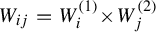 $W_{ij} = W_i^{(1)} {\times \hspace {0.5pt}} W_j^{(2)}$
, its boundary is given by
 $$ \begin{align*} \partial W^{}_{ij} = (\partial W_i^{(1)} {\times\hspace{0.5pt}} W_j^{(2)}) \cup ( W_i^{(1)} {\times\hspace{0.5pt}}\hspace{0.5pt} \partial W_j^{(2)} ) , \end{align*} $$
and consequently consists of subsets of different dimensions,
 $$ \begin{align*} d^{}_1 = \dim ( \partial W_i^{(1)}) + \dim ( W_j^{(2)} ) \quad \textrm{and} \quad d^{}_2 = \dim ( W_i^{(1)}) + \dim ( \partial W_j^{(2)} ). \end{align*} $$
This does hold for all product tile types, with the same dimensions. So, despite the unique value of the
 $\mathrm {OSD}$
, we have window boundary parts with two different dimensions.
Example 7.8. Our next example emerges from direct product variations of Fibonacci tilings [Reference Baake, Frank and Grimm8]. The ones with polygonal windows all represent topologically conjugate dynamical systems [Reference Baake, Gähler and Mazáč10], and so their
 $\mathrm {OSD}$
and window boundary dimensions are equal to those of the plain direct product of two Fibonacci tilings, namely
 $\mathrm {OSD}(\mathbb {X},\mathbb {R}\hspace {0.5pt}^2)=2$
and
 $\overline {\dim }_B(\partial W)=1$
. More interesting are the three types of systems with fractally bounded windows, which in [Reference Baake, Frank and Grimm8] were called castle, cross and island. For each type, the discrepancy inflation is primitive, with its leading eigenvalue being the largest root of the polynomials
 $$ \begin{align*} p(x) = \begin{cases} x^3-4x^2+5x-3, & \text{castle}, \\ x^9-2x^8-x^7+x^6+x^5-4x^4-2x^3-1, & \text{cross}, \\ x^5-2x^4-x^3+2x^2+x-4, & \text{island}. \end{cases} \end{align*} $$
Note that, for the second polynomial, there is a deviation from [Reference Baake, Frank and Grimm8], although the largest roots are very close numerically. This deviation still needs to be resolved. Numerically, the largest roots
 $\unicode{x3bb} _{\mathrm {dc}}$
of the polynomials are, approximately,
 $2.46557$
,
 $2.33157$
and
 $2.11978$
. For the
 $\mathrm {OSD}$
, we then get

Correspondingly, the dimensions of the window boundaries become

Thus, the
 $\mathrm {OSD}$
distinguishes these classes topologically, as stated in [Reference Baake, Frank and Grimm8] based on the window boundary dimensions.
Example 7.9. The Hat tiling [Reference Smith, Myers, Kaplan and Goodman-Strauss36] has recently attracted much attention due to its aperiodic monotile property, but it is interesting also for its
 $\mathrm {OSD}$
. We find two different Lyapunov exponents,

where
 $\phi $
is again the golden mean. These two Lyapunov exponents can also be seen in the window boundary, which has straight parts and fractal parts [Reference Baake, Gähler and Sadun7]. At first sight, this gives only upper and lower bounds on the
 $\mathrm {OSD}$
. However, the Hat tiling has a cousin, the Golden Hex Tiling (GHT) of [Reference Akiyama and Araki1], whose construction indicates that it is topologically conjugate to the Hat tiling. Indeed, we find the same two Lyapunov exponents also for the GHT. Here, the dynamical system of the GHT has a factor, which is obtained by replacing the two kinds of trapezoids by a parallelogram and a triangle each. This simplified GHT has only one Lyapunov exponent, the larger of the above two.
Since the
 $\mathrm {OSD}$
cannot increase under a factor map, the full GHT must have the same
 $\mathrm {OSD}$
as the simplified one, and if the Hat tiling is conjugate to the GHT, the same holds for the Hat tiling. As a result, we have
 $$ \begin{align*} \mathrm{OSD}( \mathbb{X}^{}_{\mathrm{Hat}}, \mathbb{R}\hspace{0.5pt}^2 ) = \frac{4\log(\phi)}{4\log(\phi) - \log (2+\sqrt{3} )} \approx 3.166{\hspace{0.5pt}\hspace{0.5pt}}443. \end{align*} $$
As shown in [Reference Baake, Gähler and Sadun7], the window boundaries consist of components with dimensions
 $$ \begin{align*} d^{}_1 = 1 \quad \textrm{or} \quad d^{}_2 = \frac{ \log(2+\sqrt{3} ) }{2\log(\phi)}, \end{align*} $$
which correspond to the two Lyapunov exponents of the Hat tiling. We see here that, despite the two different Lyapunov exponents, we can have a well-defined
 $\mathrm {OSD}$
, while the window boundary contains components of different dimensions; compare Example 7.7.
8 Concluding remarks
Barge and Diamond [Reference Barge and Diamond14] have encoded the proximality structure of one-dimensional inflation tilings with pure-point spectrum by the corresponding balanced pair discrepancy inflations,
 $\varrho ^{}_{\mathrm {dc}}$
. They have shown (under an additional no-cycle condition, which is believed to be only technical) that two tiling spaces are homeomorphic if and only if the tiling spaces generated by their respective
 $\varrho ^{}_{\mathrm {dc}}$
are homeomorphic. In [Reference Maloney and Rust31, Example 6.11], Maloney and Rust have used this to distinguish two tiling spaces which are hard to distinguish by any simpler means. Concretely, they have computed bounds on the cohomology ranks of the two spaces and could thereby tell them apart. Here,
 $\mathrm {OSD}$
encodes (in sufficiently nice situations) only the leading eigenvalue of
 $\varrho ^{}_{\mathrm {dc}}$
and is thus much simpler to compute. Nevertheless, it allows to distinguish these two spaces as well and therefore constitutes a powerful tool.
Above, we have assumed that our tilings are self-similar, with an inflation scaling
 $\unicode{x3bb} $
that is isotropic. This restriction is not essential, and, with minor adjustments, most of our results hold also in the self-affine case, where the inflation scaling is a general, strictly expanding linear map Q, whose expanding eigenvalues form a Pisot family [Reference Lee and Solomyak29]. Essentially, the volume scaling factor
 $\unicode{x3bb} ^d$
has to be replaced by
 $\lvert \det (Q) \rvert $
, as is also well known from the spectral analysis of such tilings [Reference Baake, Gähler and Mañibo9]. Some further complications might arise though, especially regarding the window boundary dimensions.
We have also assumed that our inflations are stone inflations, which means that the super-tiles are precisely dissected into copies of the original tiles, where we consider only the case where the supertiles are scaled copies of the prototiles. Solomyak’s overlap algorithm [Reference Solomyak37] also assumes this. This is more restrictive than necessary. It is enough if each tile is assigned to a unique supertile. The limiting shape of a supertile may then become fractal, which makes the overlap algorithm difficult to apply, because it may be hard to determine whether two fractal shapes do overlap. However, Akiyama and Lee [Reference Akiyama and Lee3] have developed a generalized overlap algorithm, which can cope with this situation, by considering almost overlaps. With this overlap algorithm, the
 $\mathrm {OSD}$
is straight-forward to compute.
Our approach described above can directly be applied only to self-similar (or to self-affine) tilings. Clark and Sadun [Reference Clark and Sadun17] have investigated how the spectral properties of such dynamical systems change under shape changes of the tiles. They showed that shape changes which are asymptotically negligible lead to dynamical systems that are topologically conjugate to the original one and hence do not change the
 $\mathrm {OSD}$
. Further, applying a global linear map to a tiling space is a relevant shape change, but it will also not affect the
 $\mathrm {OSD}$
. Other asymptotically non-negligible shape changes, however, will generically kill all (non-trivial) point spectra and hence change the
 $\mathrm {OSD}$
drastically (from a finite to an infinite value). Asymptotic negligibility is controlled by the cohomology class in
 $\check {H}^1(\mathbb {X},\mathbb {R}\hspace {0.5pt}^d)$
of a shape change [Reference Clark and Sadun17].
In a sense,
 $\mathrm {OSD}$
and Čech cohomology [Reference Anderson and Putnam4] of the underlying tiling space are complementary complexity measures. Both depend on the set of singular fibres over the MEF. The complexity of Čech cohomology comes from the multiplicity of the singular fibres, which is completely irrelevant for
 $\mathrm {OSD}$
, as all tilings in a fibre are identified. Rather,
 $\mathrm {OSD}$
depends on the geometry of the set of singular fibres. The two complexity measures therefore see different origins of complexity and complement each other.
In the case where we have a Lyapunov spectrum with several values, we may be able to say more than giving the rough bounds of Theorem 4.10, as we saw in Example 7.7. In other examples like the Hat tiling [Reference Baake, Gähler and Sadun7, Reference Smith, Myers, Kaplan and Goodman-Strauss36], the larger of two Lyapunov exponents seems to be the relevant one. In this area, better criteria are still needed.
Acknowledgements
It is our pleasure to thank Maik Gröger for illuminating discussions, and Henk Bruin, Natalie Frank and Karl Petersen for helpful comments. This work was supported by Deutsche Forschungsgemeinschaft (DFG, German Research Foundation), via TRR 358/1 2023–491392403 (M.B., F.G.) and Project 509427705 (P.G.).