







1. Introduction
The mixing of fluids with differing densities in response to acceleration belongs to a family of instabilities known as the Rayleigh–Taylor (RTI) and Richtmyer–Meshkov instabilities (RMI). These instabilities result from the deposition of baroclinic vorticity along an interface where the density gradient caused by the differing properties of the two fluids is mis-aligned with the pressure gradient caused by the acceleration of the fluids. The RTI (the case resulting from a finite, sustained acceleration) was first described by Rayleigh (Reference Rayleigh1882) and later extended by Taylor (Reference Taylor1950). The RMI (the case resulting from an impulsive acceleration, such as that caused by the passage of a shock wave) derives its name from the early analytical work of Richtmyer (Reference Richtmyer1960) and the later experimental verification by Meshkov (Reference Meshkov1972). The RMI is of importance in natural astrophysical phenomena, where it results in the mixing of accelerated stellar gases in planetary nebulae (Arnett et al. Reference Arnett, Bahcall, Kirshner and Woosley1989), as well as in furthering our understanding of fundamental flow physics. It has found limited technological application, but has been found relevant to the enhancement of the mixing of fuel and air in supersonic combustion ramjet engines (Yang, Kubota & Zukoski Reference Yang, Kubota and Zukoski1993). The RMI is also a major hindrance to the efforts of the ignition campaign at the National Ignition Facility, where many instabilities including the RMI result in the mixing of shell material into the hot core of the imploding capsule, which quenches the fusion through radiative cooling in a phenomenon known as the ‘mix cliff’ (Zhou Reference Zhou2017a,Reference Zhoub).
Many shock tube experiments (such as the early work by Meshkov) relied on thin membranes to separate the experimental gases. The use of membranes provides excellent control over the shape of the initial perturbation, while also ensuring excellent repeatability and a sharp interface between the experimental gases (Vetter & Sturtevant Reference Vetter and Sturtevant1995). The membrane is obliterated by the passage of the shock wave. However, the remaining fragments have a damping effect on the ensuing RMI due their high inertia. The fragments also inhibit the free mixing of the experimental gases. In order to circumvent this deleterious behaviour, most modern shock tube experiments have moved towards the formation of a membraneless interface, either using a counterflow configuration (Jones & Jacobs Reference Jones and Jacobs1997; Collins & Jacobs Reference Collins and Jacobs2002; Weber et al. Reference Weber, Haehn, Oakley, Rothamer and Bonazza2012; Reese et al. Reference Reese, Oakley, Navarro-Nunez, Rothamer, Weber and Bonazza2014; Mohaghar et al. Reference Mohaghar, Carter, Pathikonda and Ranjan2019) or using some form of gas curtain (Jacobs et al. Reference Jacobs, Jenkins, Klein and Benjamin1995; Balakumar et al. Reference Balakumar, Orlicz, Tomkins and Prestridge2008). Membraneless experiments also allow the use of modern laser based diagnostic techniques such as particle image velocimetry (PIV) and plane laser induced fluorescence (PLIF) which further enhances the analysis capabilities of experimental studies. Early experiments using membranes relied only on schlieren or shadowgraph imaging, which limited the capacity of these experiments to accurately measure the mixing layer width. Much of the early experimental work on membraneless experiments, such as the work of Jones, focused on creating a two-dimensional sinusoidal perturbation with one dominant mode. These excitations, achieved by horizontal oscillation of the tube, allowed for very precise and repeatable initial conditions, enabling time series to be assembled from a single image per experiment (a limitation of the visualization systems of the time).
More modern experiments focus on the creation of a broadband initial perturbation to better explore the late-time turbulent evolution of the RMI. One of the most important parameters in these types of experiments is the characterization of the scaling of the interface width, and the growth behaviour in the late-time self-similar regime. While the late-time growth behaviour for RMI driven flows is less well established than that corresponding to the RTI, there is a general consensus that a power law  $h(t) \propto t^\theta$ (where h is the interface thickness and t is time) appears to describe the growth of the mixing layer width for the case of the turbulent, self-similar instability. A wide variety of
 $\theta$ values have been reported and predicted in various simulations and models (Zhou Reference Zhou2017a,Reference Zhoub), yet there is relative paucity of experimental data which are suitable for extracting
 $\theta$ values. Of the experiments which have been carried out, a range of
 $\theta$ values have been found. The early experiments of Dimonte, Frerking & Schneider (Reference Dimonte, Frerking and Schneider1995) report
 $\theta \approx 0.6$, while later experiments (Dimonte & Schneider Reference Dimonte and Schneider1997, Reference Dimonte and Schneider2000) find much lower values around
 $\theta \approx 0.25\text {--}0.43$. The early experiments were performed on solid density materials using the Nova laser facility, and rely on the diagnostically challenging radiography method to produce their measurements, with the most recent experiments utilizing backlit photography and laser induced fluorescence. The experiments of Prasad et al. (Reference Prasad, Rasheed, Kumar and Sturtevant2000) report
 $\theta$ in the range
 $0.26\text {--}0.33$ from experiments performed in a large shock tube, however, these experiments are hampered by the combined use of schlieren imaging with a membrane to produce the initial perturbation, and the data are comprised of relatively few measurements, which increases the difficulty of fitting a power law to the data. The recent experiments of Weber et al. (Reference Weber, Haehn, Oakley, Rothamer and Bonazza2012, Reference Weber, Haehn, Oakley, Rothamer and Bonazza2014) measured
 $\theta$ in the range
 $0.43\text {--}0.58$ using the fluorescent signal from an acetone tracer on a shocked broadband interface generated by a turbulent cross-flow forcing technique. Finally, the experiments of Jacobs et al. (Reference Jacobs, Krivets, Tsiklashvili and Likhachev2013) measure
 $\theta$ in a shock tube most similar to the present experiment using Mie scattering and report
 $\theta$ in the range
 $0.3\text {--}0.4$.
In order for experiments to accurately capture the turbulent growth behaviour of the late-time self-similar RMI, a broad spectrum of modes must be imposed on the initial interface, with as little low mode content as possible. If the interface between the two gases is well defined (capable of being described by a single valued function), the initial growth of the mixing layer width can be described as a linear superposition of the modal content of the perturbation with each mode following  $\dot {h}=A V_0 \eta k$, where
 $A$ is the Atwood number,
 $V_0$ is the post-shock velocity,
 $\eta$ is the amplitude of the particular mode having wavenumber
 $k$. High frequency modes grow quickly and become saturated rapidly, retarding the growth of the mixing region. The presence of long wavelength, low wavenumber modes then dominates the growth of the interface for the duration of any practical experiment. The modal content of the initial perturbation has a strong impact on the growth of RMI, and can help to explain the large variation in the experimentally reported values of
 $\theta$. The simulations of Thornber et al. (Reference Thornber, Drikakis, Youngs and Williams2010) and Tritschler et al. (Reference Tritschler, Olson, Lele, Hickel, Hu and Adams2014) exemplify the effect of the initial condition bandwidth on the growth of the RMI. The two simulations were initialized in a very similar manner but with different modal content. The narrow band, short wavelength perturbations of Thornber's simulations produce a smaller
 $\theta$ value than the broader band, longer wavelength perturbations of Tritschler's simulations. The simulations of the
 $\theta$-Group (Thornber et al. Reference Thornber2017) use a narrowband initial perturbation similar to that of Thornber et al. (Reference Thornber, Drikakis, Youngs and Williams2010) with similar result. On the other hand, Gowardhan, Ristorcelli & Grinstein (Reference Gowardhan, Ristorcelli and Grinstein2011) employ initial perturbation spectra ranging from something similar to Thornber et al. (Reference Thornber, Drikakis, Youngs and Williams2010) to those with more broadband characteristics and find two different behaviours: one exhibiting near linear growth when initiated with a low-amplitude initial perturbation and another exhibiting power-law growth with
 $\theta \approx 0.5$ when simulations were initiated with a much higher-amplitude perturbation. In general, simulations initialized with narrowband perturbations tend to produce much smaller
 $\theta$ values than those reported in experiments, a fact which can likely be attributed to the short wavelength small bandwidth perturbations which are most often used when simulating the RMI.
Generating interfaces experimentally relies on non-repeatable and stochastic processes, such as the Faraday forcing in the experiments of Jacobs et al. (Reference Jacobs, Krivets, Tsiklashvili and Likhachev2013), and the experiments which utilize cross-flow jets such as Mohaghar et al. (Reference Mohaghar, Carter, Musci, Reilly, McFarland and Ranjan2017), Weber et al. (Reference Weber, Haehn, Oakley, Rothamer and Bonazza2012, Reference Weber, Haehn, Oakley, Rothamer and Bonazza2014) and Reese et al. (Reference Reese, Oakley, Navarro-Nunez, Rothamer, Weber and Bonazza2014). These types of perturbations present additional experimental challenges due to the uniqueness of each initialization or initial condition. This class of experiments benefits greatly from time resolved measurements, as the small differences in the initial forcing conditions can alter the development of the RMI, making ensembles of experiments less useful. Accurate estimation of  $\theta$ requires estimation of the curvature of the width of the growing perturbation, and the additional data points obtained in experiments with high time fidelity produces much more reliable results when obtaining
 $\theta$ values from individual experiments. One observation in the experiments of Jacobs et al. (Reference Jacobs, Krivets, Tsiklashvili and Likhachev2013) which was detected with the aid of high time fidelity was the observation of a bifurcation in the growth exponent. This difference in
 $\theta$ was conjectured to have been caused by the inversion of the perturbation during Faraday forcing resulting in experiments having large differences in initial amplitude. During these experiments the timing of the shock arrival was not controlled, resulting in shock interaction with the interface at a random phase of the forcing cycle and a consequent variation in the initial amplitudes.
There exist very few experimental studies performed with initial conditions suitable for comparison with simulations of the self-similar growth of RMI such as that by Thornber. In addition, there are even fewer that lack the deleterious effects of membranes used to form the initial perturbation. Thus, this work is meant to provide measurements that could be used for comparison with existing or future numerical studies. The experiments presented here seek to provide robust measurements of  $\theta$, and to characterize the results of the late-time growth through the observation of turbulent quantities such as the anisotropy of the mixing layer turbulence, the growth of turbulent length scales and the spectra of the turbulent kinetic energy. Another goal of this work is to investigate the effect of amplitude of the Faraday wave generated initial perturbation on the growth of the RMI. The sinusoidal forcing of the gas–gas interface results in the formation of waves which invert at half the forcing frequency, caused by the Rayleigh–Taylor unstable baroclinic torque deposited during the unstable acceleration during interface excitation. To investigate the effect of initial amplitude on the growth of the instability, the experiments are separated into two groups: high-amplitude experiments where the shock wave arrives near the maximum excursion of the perturbation, and low-amplitude experiments where the shock arrives near the inflection point. The experiments are quantified using planar PIV, which provides a quantitative two-dimensional velocity field at the centre plane of the shock tube. This diagnostic enables the measurement of the growth parameter
 $\theta$, as well as investigation of turbulent phenomena such as anisotropy and the evolution of turbulent length scales and the turbulent mixing transition.
The current work is presented in the following sections. Section 2 provides a description of the experimental apparatus and test facility, as well as a discussion of the experimental excitation and diagnostics. Section 3 analyses the results of the experiments, discussing the growth of the mixing layer, anisotropy, turbulent length scales, mixing transition and spectral quantities. Section 4 gives the discussion and conclusions of the study.
2. Experimental set-up
2.1. Apparatus description
The experiments were performed at the University of Arizona Fluid Instabilities Laboratory. Figure 1 shows a schematic representation of the shock tube used. The tube is 9 m long, and is comprised of three sections: a round, 3.7 m long wound fibreglass driver section, coupled to a square 4.1 m long fibre reinforced plastic driven section, and a 1.2 m long clear acrylic test section. The driven and test sections have a square inner cross-section of 8.9 cm, and are coupled to a 10.2 cm diameter wound fibreglass driver using fibre reinforced plastic flanges. The shock tube design is similar to the membraneless shock tube pioneered by Jones & Jacobs (Reference Jones and Jacobs1997) and Collins & Jacobs (Reference Collins and Jacobs2002), and reported most recently by Jacobs et al. (Reference Jacobs, Krivets, Tsiklashvili and Likhachev2013).
Schematic illustration of the shock tube showing the lengths of the main three sections of the apparatus, and the relative locations of the various components.

A membraneless interface is formed in a similar manner to Jones, using a counter-flow configuration where the light gas (air) flows into the driven section from an inlet approximately 1 m above the interface location, and the heavy sulphur hexafluoride (SF $_6$) gas flows in from a plenum located in the bottom of the tube. This gas combination results in an Atwood number (
 $A=(\rho _2-\rho _1)/(\rho _2+\rho _1)$ where
 $\rho _2$ and
 $\rho _1$ are the heavy and light gas densities, respectively) of 0.67. Both gases flow at a matched volumetric rate of 6 l min
 $^{-1}$ and are allowed to exit from a series of small holes drilled in the test section. This causes the formation of a stable, diffuse, stratified interface at the location of the holes. The driver section is pressurized to approximately 220 kPa and the
 $\sim$2
 $\mathrm {\mu }$m thick polypropylene diaphragm separating the driver and driven sections is ruptured using a solenoid driven firing mechanism, resulting in the formation of a Mach 1.17 shock wave travelling in the downward (
 $+x$) direction, where it interacts with the interface. The shock wave reflects from a configurable false wall in the bottom of the tube and interacts with the interface a second time (reshock) approximately 4.5 s after the initial shock interaction. The false wall is constructed from a stack of 25.4 mm thick Acrylonitrile Butadiene Styrene (ABS) plastic plates, which is installed in the bottom of the tube. The false wall allows the effective length of the test section to be shortened, adjusting the time of the reflected shock wave arrival.
2.2. Interface excitation
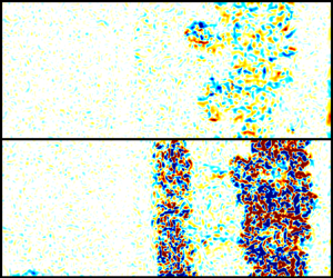
Perturbations are excited via vertical oscillation of the gas column at a frequency of approximately 24 Hz using a pair of voice coil drivers located near the bottom heavy gas plenum and at the top of the driven section. The vertical oscillation results in the formation of Faraday waves on the interface between the two gases. The Faraday forcing generates a broadband, three-dimensional perturbation. Faraday waves invert at double the period of the forcing frequency, and the initial amplitude for the experiments is controlled by rupturing the membrane at a precise time relative to the phase of the actuation signal. Two groups of experiments are presented – ‘high amplitude’ experiments where the amplitude of the initial perturbation is maximized, and ‘low amplitude’ experiments where the perturbation is near its inflection point. Example images of high and low-amplitude perturbations are shown in figure 2. Images of the perturbation just prior to shock wave arrival were processed to obtain a line representing the initial interface location. The images of the perturbation are first convolved with a Gaussian weighted 10 pixel square kernel to average the bright signal created by individual particles, and create a smoothed image where the two gases appear with different intensity levels. A Sobel filter is then used to detect gradients in the smoothed images, rendering the interface between the gases as a bright line. A threshold is then applied to the Sobel filtered image to create a binary image, from which a line that approximates the interface location can be traced. From this line, the initial amplitude and frequency content of the perturbation was determined. High amplitude experiments were found to have a root-mean-square (r.m.s.) amplitude  $\overline {h_{0h}} \approx 1.7 \pm 0.3$ mm with low amplitude experiments having an initial amplitude of
 $\overline {h_{0l}} \approx 0.8 \pm 0.3$ mm. Average spectra of the interface line for high and low-amplitude experiment initializations are shown in figure 3.
Example raw PIV images showing the initial perturbations just before shock arrival for (a) high-amplitude (EX02) and (b) low-amplitude (EX12) experiments.

Mean and envelope of spectral power for (a) high-amplitude and (b) low-amplitude experiments.

2.3. Diagnostics
The diagnostic technique employed in this study is PIV, which uses the motion of particles seeded in the flow to produce quantitative planar measurements of velocity. The particles were produced by evaporation of a mixture of glycerol and propylene glycol at a 50–50 ratio. The seeder consists of a small Buchner flask containing the seed fluid, with a length of wound FeCrAl (Kanthal) wire forming a heating element with an approximate resistance of 0.5 $\varOmega$. The seed fluid is wicked to the heating element using 3 mm silica rope, and the heater is powered at approximately 1.25 watts to produce an appropriate seeding level for PIV. The particles were sized in situ by measuring their response to shock acceleration and found to have an average size of
 $\sim$1.6
 $~\mathrm {\mu }$m.
The particles are illuminated using a Photonix DM-70 YLF laser, which is collimated and steered into the test section axially from the bottom. The beam is focused using a cylindrical lens with a long focal distance, with the beam waist coinciding with the measurement location. The beam is spread into a sheet using a concave cylindrical lens, and passes through a fused silica window located in the shock tube end wall. The thickness of the laser sheet throughout the measurement area is  $<$1 mm. Images are captured using three Photonix APX-RS high speed cameras fitted with 105 mm Nikon Micro-Nikkor f/2.8 AF lenses (resulting depth of field 2 cm). The cameras are operated in double-frame mode capturing image pairs at a rate of 2000 Hz with an imaging area of 1024 by 784 pixels, resulting in a particle image pixel pitch of 125
 $\mathrm {\mu }$m px
 $^{-1}$.
The particle images were processed using Lavision's DaVis software, employing an iterative, multi-pass algorithm with an adaptive window used in the final pass. The minimum window size of 16 by 16 pixels with 75 % overlap results in a final vector spacing of 500  $\mathrm {\mu }$m. The individual vector fields are then stitched together resulting in a final measurement field of 680 by 164 vectors covering 33.6 by 8.0 cm. Spurious vectors are detected and removed using the universal outlier detection described by Westerweel & Scarano (Reference Westerweel and Scarano2005). On average, 98 % of first-choice vectors were kept, with the rejected vectors being removed and replaced by alternate choices using the universal outlier detection algorithm. Combined r.m.s. error from the correlation statistics method (Wieneke Reference Wieneke2015) and peak locking is found to be
 $\sim$0.6 m s
 $^{-1}$. Due to the random nature of the error it does not significantly affect aggregate measures such as mean velocity fields, and only has a minor effect on measures such as turbulent kinetic energy (TKE) (which varies by
 $\pm$0.02 %).
2.4. Experimental runs
Sixteen total experiments were performed on a perturbed air/SF $_6$ interface (
 $A=0.67$) with a shock Mach number of
 $1.17\pm 0.002$. Nine experiments were conducted at high amplitude, with the remaining seven experiments being conducted with low-amplitude perturbations. After shock interaction, the interface grows undisturbed for
 $\sim$4.5 ms, whereupon the reflected shock wave returns and interacts with the interface a second time (reshock). After the second shock interaction, the interface is observed for another
 $\sim$2.5 ms until the arrival of a reflected expansion wave accelerates the interface, ending the pure Richtmyer–Meshkov (RM) growth phase. A montage showing the vorticity field of a full experimental run is shown in figure 4. The figure qualitatively shows the decay in vorticity with time, in addition to illustrating the dramatic increase in vorticity following reshock. Panel (a) shows the interface a short time after shock interaction (0.27 ms). The reflected shock wave is observable in frames (
 $j,k$), where the shock wave is noticeably thickened after interaction with the growing interface. The shock wave is observable in the PIV due to the differential acceleration particles which are relatively larger or smaller than their neighbours. Post-reshock, the increase in TKE is readily observable, along with a reduction in the average size of turbulent eddies.
A sequence of vorticity fields obtained from PIV processing of a typical experiment (high-amplitude experiment 2) at (a)  $t = 0.27$ ms, (b)
 $t = 0.77$ ms, (c)
 $t = 1.27$ ms, (d)
 $t = 1.77$ ms, (e)
 $t = 2.27$ ms, (f)
 $t = 2.77$ ms, (g)
 $t = 3.27$ ms, (h)
 $t = 3.77$ ms, (i)
 $t = 4.27$ ms, (j)
 $t = 4.77$ ms, (k)
 $t = 5.27$ ms, (l)
 $t = 5.77$ ms, (m)
 $t = 6.27$ ms, (n)
 $t = 6.77$ ms. Reshock occurs at
 $\sim$4.6 ms.

3. Data analysis and results
3.1. Mixing layer growth
The growth of the RMI has long been assumed (Alon et al. Reference Alon, Hecht, Mukamel and Shvarts1994) to follow a power-law behaviour of the form  $h\propto C(t-t_0)^\theta$. Experiments and simulations have observed a wide range of growth exponents
 $\theta$, from
 $\theta =0.18$ on the low end to as high as
 $\theta = 0.62$ (Zhou Reference Zhou2017a) depending on the parameters of the experiment or computation. Barenblatt (Reference Barenblatt1983) showed that for self-similar, Boussinesq (low Atwood number) flow with no dissipation (constant kinetic energy) that
 $\theta =2/3$. For dissipative flows, if the kinetic energy decays according to a power law TKE
 $=kt^{-q}$, Thornber et al. (Reference Thornber, Drikakis, Youngs and Williams2010) have shown that
 $\theta$ can be related to the kinetic energy decay exponent
 $q$ by the relation
 $\theta =(2-q)/3$.
 $\theta$ is important to estimate as it is generally accepted to be the most fundamental parameter describing self-similar RMI growth. It is typically not calculated following reshock particularly because most shock tube RMI experiments have very limited experimental time to observe the interface following reshock (a problem which is not well addressed in these experiments). However, it is our belief that the power-law growth expression should be appropriately applied there as well. Note that it is sometimes assumed that the value of
 $\theta$ should be universal for a fully turbulent self-similar RMI. Thus, there is no reason to expect reshock to be different from the singly shocked instability. We therefore think it important to make the best analysis possible following reshock.
Due to the sparse nature of the seeding for the PIV diagnostic, the turbulent mixing layer (and therefore its width) is not directly observable throughout the course of the experiment. Instead, we calculate  $\theta$ by measuring the spread of TKE, positing that the energetic turbulence of the mixing layer coincides with the location of the mixing region. An estimation of the turbulent kinetic energy is made here using the following definitions: TKX
 $=\sum _{xy} \frac {1}{2}(u-\bar {u})^2)$, TKY
 $=\sum _{xy} \frac {1}{2}(v-\bar {v})^2)$, TKE=TKX+TKY+TKZ where TKZ=TKY due to assumed homogeneity in the spanwise and out of plane directions. Fluctuating quantities are determined on a per-row basis, where the mean velocity of each row in the spanwise (
 $y$) direction is subtracted. Figure 5 shows the method of calculating width for a typical frame. Using the spanwise (
 $y$) mean of TKE, we calculate a threshold based on 5 % of the peak TKE in the spanwise mean, and use this to find the edges of the mixing region. The difference between these points is taken as the width (
 $h$). The centroid of the spanwise mean (calculated as
 ${\int x f(x) {\textrm {d}x}}/{\int f(x) {\textrm {d}x}}$ where
 $f(x)$ is the spanwise average of the TKE field) is also used as the centreline of the growing mixing layer.
A typical kinetic energy field from a single frame (a). The transverse mean of the kinetic energy field (b) with centroid and thresholded bounds used for calculating the width of mixing region.

Profiles of  $h$ vs time are shown in figure 6. The value of
 $\theta$ is found for each experiment individually using nonlinear least squares regression to the form
 $min(\varSigma ||F(x_i)-y_i||^2)$ where
 $F(x_i)$ is a nonlinear function (in this case
 $F(x_i)=h=Ct^\theta$) and
 $y_i$ are data, with bi-square weighting (a method which seeks to diminish the effect of outlier data by minimizing a weighted sum of squares, where the weight given to each data point depends on how far the point is from the fitted line). The quality of fitting was evaluated through 95 % confidence intervals of the fitted coefficients. These were obtained using the confidence interval functionality of MATLAB's curve fitting toolbox, which uses the inverse
 $R$ factor from QR decomposition of the Jacobian, the degrees of freedom for error and the r.m.s. error to estimate an interval. This analysis gives an estimation of the error in the computed value of
 $\theta$ due to sampling error (frame to frame variations in the width which arise when structures enter or leave the plane of measurement) and whether or not the growth of the interface truly exhibits power-law type behaviour. Confidence in fits to individual experiments is high following the incident shock for high- and low-amplitude experiments, with decreasing confidence in the reshocked results due to the limited number of unaccelerated samples post reshock (before the arrival of the reflected rarefaction wave). A 95 % confidence interval of the mean value of
 $\theta$ is computed (
 $CI = t^*({s}/{\sqrt {n}})$, where
 $t^*$ is Student's
 $t$ variable,
 $s$ is the standard deviation of the computed
 $\theta$ values and
 $n$ is the sample size) and are shown in table 1. These statistics give an indication of how much run to run variation exists in the experimental set, caused by inconsistency in the initial forcing, variation in shock speed and other environmental variables. Low-amplitude experiments are less consistent than high-amplitude experiments following the initial shock, likely due to the additional sensitivity in starting amplitude due to timing jitter (the perturbation is at its highest velocity near the inflection point, and small timing errors result in larger differences in the perturbation amplitude at shock arrival).
Interface width ( $h$) based on the full width of the kinetic energy vs time for (a) high-amplitude experiments and (b) low-amplitude experiments.

Statistics for fits of  $\theta$ to the spread of TKE width and TKE decay.

A plot of all experimental runs in logarithmic scale is shown in figures 7 and 8, along with a line representing the mean value of  $\theta$ from individual fits. When fitting to the ensemble (i.e. fitting all experiments simultaneously), the value of
 $\theta$ found is very similar to the averaged
 $\theta$ obtained when fitting the experiments individually. After the passage of the second shock wave, there is a brief period of time where the mixing layer compresses and inverts before it resumes its growth, which is readily observed in figure 6(a,b), and can also be observed by the departure from the fitted curve for the early time points in figures 7(b) and 8(b). This compression and inversion is observed much more clearly in high fidelity simulations such as in those of Thornber et al. (Reference Thornber, Drikakis, Youngs and Williams2011) and Tritschler et al. (Reference Tritschler, Olson, Lele, Hickel, Hu and Adams2014). In comparing measured
 $\theta$ values for the two sets of experiments the effect of the perturbation amplitude on the growth exponent after a single shock interaction appears to be small, with low amplitude experiments exhibiting
 $\theta \sim 0.06$ lower than the high-amplitude experiments, similar to the bifurcated results observed in the work of Jacobs et al. (Reference Jacobs, Krivets, Tsiklashvili and Likhachev2013) where the initial condition phase was uncontrolled. The
 $\theta$ values following reshock are much more pronounced between the low- and high-amplitude experiments, with high-amplitude experiments demonstrating a growth exponent of
 $\theta \approx 0.33$, compared to low-amplitude experiments which continue to grow with
 $\theta \approx 0.5$. A plausible explanation for this difference is that the low-amplitude experiments, being less turbulent at the time of reshock, may contain steeper density gradients during interaction with the second shock. This would result in more energetic shock interaction with the mixing layer, and enhanced growth following reshock. In order to quantify this effect, a non-dimensional time
 $\tau =k u'_{rms|c}t$ and a non-dimensional mixing layer width
 $kh$ were used, where
 $k$ is the wavenumber of the initial perturbation and
 $u'_{rms|c}$ is the streamwise root mean square centreline velocity. Figure 9(a) shows mixing layer width in these non-dimensional variables, and reveals that in addition to a slightly retarded growth rate, the low-amplitude experiments have grown significantly less than their counterparts at the arrival of reshock. This lack of development for low-amplitude experiments can explain the differences in the reshocked growth exponents. Figure 10 shows post-reshock measured
 $\theta$ values as a function of dimensionless time at reshock, which demonstrates how measured
 $\theta$ correlates with instability development prior to reshock. The negative slope of the regression line fit to the data indicates that smaller
 $\theta$ values correlate with greater pre-reshock development. When non-dimensionalizing the reshocked data in a similar fashion (figure 9b), the dimensionless coordinates make it clear that the low-amplitude reshock case agrees well with both incident shock cases, confirming that they have similar growth behaviour and thus yield similar
 $\theta$ values. On the other hand, the non-dimensionalized high-amplitude reshock data fall well below those of the other three cases, which is consistent with the lower
 $\theta$ value obtained for this case.
Logarithmic plots of h vs time for the high-amplitude experiments following the incident shock interaction (a) and following reshock (b). The dashed lines represent curve fits to the ensemble data. The growth exponents shown were computed from the mean of individual experimental runs. Also shown are the 95 % confidence intervals of the mean.

Logarithmic plots of h vs time for the low-amplitude experiments following the incident shock interaction (a) and following reshock (b). The dashed lines represent curve fits to the ensemble data. The growth exponents shown were computed from the mean of individual experimental runs. Also shown are the 95 % confidence intervals of the mean.

Growth of the mixing layer in dimensionless coordinates for high- and low-amplitude experiments following the initial shock (a), and with added points for reshock (b).

Post reshock  $\theta$ vs non-dimensional time in the frame just prior to reshock. High-amplitude experiments which exhibit a larger non-dimensional time (i.e. a more developed state) at reshock result in lower growth exponents following reshock. The negative slope of the regression (black dashed line), indicates that low post-reshock
 $\theta$ correlates with large non-dimensional time (a well-developed mixing region) before the arrival of reshock.

Barenblatt (Reference Barenblatt1983) showed that for a Boussinesq (i.e. small Atwood number), self-similar flow with constant kinetic energy that the product  $h\dot {h}^2$ is constant, and therefore the mixing layer width should grow according to
 $h=C(t-t_0)^{2/3}$. Thus, with no dissipation and
 $A \ll 1$,
 $\theta$ is expected to be
 $2/3$. Dissipation causes TKE to decay with time, and an increase in dissipation will produce a consequent reduction in the value of
 $\theta$. Recent work by Thornber et al. (Reference Thornber, Drikakis, Youngs and Williams2010) suggests that a relationship exists between the growth rate of the mixing layer width and the decay of kinetic energy. They have shown that the total fluctuating kinetic energy is proportional to the width of the mixing layer multiplied by the mean kinetic energy. Assuming that
 $h \propto t^\theta$ and that the mean kinetic energy is proportional to
 $\dot {h}^2$, they obtain TKE
 $(t)\propto t^{3\theta -2}$. Using this method to obtain estimates of
 $\theta$ is advantageous because it is an integral quantity, and is less likely to be influenced by the presence of large flow structures at the edges of the mixing layer (a common problem encountered when making edge based measurements of the width of the mixing region).
Plots of the decay of kinetic energy are shown in figures 11 and 12. TKE decay is not observed at early times, when the developing mixing layer has not yet generated a full range of scales. In order to avoid fitting to not fully developed measurements, points are only fitted for dimensionless time  $k\dot {h}t > 1$, after which time most experiments are observed to begin to decay.
 $\theta$ is obtained for each experimental run individually, with statistics on the mean
 $\theta$ value shown in table 1. Good agreement is observed between the TKE width measurements and TKE decay measurements for high-amplitude experiments following the interaction with the first shock, with both methods yielding
 $\theta \sim 0.51$. Agreement following reshock is less favourable, though the measurements do have overlapping confidence intervals. We obtain the expected
 $\theta \sim 2/3$ value for non-dissipative flows in low-amplitude pre-reshock measurements using the TKE decay method, yet calculate much lower values when measuring the width of the TKE region. The disagreement may be caused by a violation of some core assumption in Thornber's model, such as the requirement that the flow be self-similar. Thornber et al. (Reference Thornber, Drikakis, Youngs and Williams2010) found
 $\theta \sim 0.26$ after interaction with the initial shock, and
 $\theta \sim 0.28$ following a second shock interaction for simulations performed with a narrow-band initial perturbation. Tritschler et al. (Reference Tritschler, Olson, Lele, Hickel, Hu and Adams2014), using a broad-band perturbation with an added dominant wavelength that is more similar to the perturbation used in the experiments presented here, found
 $\theta \sim 0.58$ after the initial shock passage and
 $\theta \sim 0.29$ following reshock. Similarly, Gowardhan et al. (Reference Gowardhan, Ristorcelli and Grinstein2011) found
 $\theta \sim 0.5$ for their high-amplitude experiments with perturbations ranging from narrow to broadband.
Logarithmic plots of kinetic energy decay vs time for the high-amplitude experiments following initial shock interaction (a) and following reshock (b). Here,  $\theta$ is computed from the mean fit to individual experimental runs. Also shown is the 95 % confidence interval of the mean. Omitted data points with
 $k_0\dot {h}_0t<1$ are shown with red
 $x$.

Logarithmic plots of kinetic energy decay vs time for the low-amplitude experiments following initial shock interaction (a) and following reshock (b). Here,  $\theta$ is computed from the mean fit to individual experimental runs. Also shown is the 95 % confidence interval of the mean. Omitted data points with
 $k_0\dot {h}_0t<1$ are shown with red
 $x$.

3.2. Anisotropy
Persistent anisotropy is widely observed during late time RMI evolution in previous experiments and simulations. It is expected that the flow should be anisotropic during the early stages of development, as the bulk of the motion imparted by the passage of the shock wave is in the streamwise direction. As the flow transitions into the nonlinear turbulent phase, the anisotropy ratio (the ratio of fluctuating kinetic energy TKX/TKY) is frequently observed to asymptote to a constant value (Thornber et al. Reference Thornber, Drikakis, Youngs and Williams2010; Tritschler et al. Reference Tritschler, Olson, Lele, Hickel, Hu and Adams2014; Oggian et al. Reference Oggian, Drikakis, Youngs and Williams2015; Thornber et al. Reference Thornber2017). A constant value of the anisotropy ratio is expected for self-similar flows; self-similar decay suggesting that all three velocity components are decaying at the same rate. The anisotropy ratio is plotted for all experiments in figure 13, with a moving average filter illustrating the mean behaviour. High-amplitude experiments are observed to asymptote to an approximate value of  $\sim$1.88 approaching reshock, with a slight rise after reshock followed by a downward trend, indicating that the mixing region after the reshock is becoming more homogeneous. Low-amplitude experiments are not observed to asymptote during the span of the experiment, with the decreasing value indicating that the initially high streamwise energy is still being converted to cross-stream energy via mode coupling as the flow evolves. Thornber et al. (Reference Thornber, Drikakis, Youngs and Williams2010, Reference Thornber2017) noticed similar behaviour to the high-amplitude experiment set in his simulations, reaching an asymptotic value of
 $\sim$1.52 after the initial shock, with an increased value of
 $\sim$1.7 following reshock. This is somewhat counter-intuitive, as it is expected that the intensified turbulence following a second shock interaction would result in the mixing layer becoming more homogeneous rather than less.
Anisotropy ratio (TKX/TKY) for the high-amplitude (a) and low-amplitude (b) experiments. Constant anisotropy ratio, as observed in high-amplitude experiments before the arrival of reshock, is a necessary but not sufficient condition for self-similarity.

The spatial distribution of anisotropy in the mixing layer can also be investigated using the Reynolds anisotropy tensor, defined as  $b_{ij}={\overline {u_i u_j}}/{k} - {\delta _{ij}}/{3}$,
 $k={\overline {u_i u_i}}/{2}$. The diagonal components (
 $b_{11},b_{22}$) of the tensor represent energy in the primary flow directions
 $x$ and
 $y$ respectively, and are bounded between
 $-\frac {1}{3}$ and
 $\frac {2}{3}$ with a trace of zero. The symmetric off-diagonal components are bounded by
 $\pm \frac {1}{2}$ and are non-zero when shear is present in the flow. Spanwise (
 $y$) averaged profiles are ensemble averaged relative to their centreline coordinate
 $x_c$ and are shown in figure 14. These profiles show strong anisotropy in the centre of the mixing layer, decaying towards the edges immediately after first shock interaction for both the high and low-amplitude experiments. At the intermediate time (before reshock) the anisotropy becomes well distributed in high-amplitude experiments, while low-amplitude cases exhibit a larger amount of anisotropy overall. Also, the heavy gas side (positive coordinate in figure 14) in the low-amplitude experiments develops a slightly higher degree of anisotropy at the intermediate time. Similar asymmetry was observed in the numerical simulations of Tritschler et al. (Reference Tritschler, Olson, Lele, Hickel, Hu and Adams2014). Reshock brings the flow in both cases to a similar average level of anisotropy, though the asymmetry observed in the low-amplitude experiments is still faintly present in the reshocked flow. Mohaghar et al. (Reference Mohaghar, Carter, Musci, Reilly, McFarland and Ranjan2017, Reference Mohaghar, Carter, Pathikonda and Ranjan2019) observe similar levels and distribution of anisotropy in their inclined shock tube experiments.
Ensemble streamwise profiles of elements of the anisotropy tensor  $b_{ij}$. Profiles are averaged relative to the centreline of the mixing region (
 $x$–
 $x_c$), where the positive
 $x$-direction is towards the heavy gas side. The high (a,c,e) and low (b,d,f) amplitude profiles are shown at the earliest time following shock interaction (0.27 ms - a,b), the latest time before reshock (4.27 ms - c,d) and the latest time following reshock (6.77 ms - e,f).

The mean of the diagonal elements of the anisotropy tensor averaged in time and across the mixing layer are shown in figure 15. Anisotropy is initially high following shock interaction, with high-amplitude experiments exhibiting a slightly larger average anisotropy due to the larger interpenetration speeds of the growing layer at the earliest times. The high-amplitude experiments, which are driven harder by the shock interaction, quickly fall to the asymptotic value. Mode coupling occurs more quickly in these experiments, which are at a higher overall energy. Following reshock, both experiments are brought to similar levels of anisotropy.
Ensemble mean of the diagonal elements of the anisotropy tensor across the mixing layer vs non-dimensional time. Blue lines indicate high-amplitude experiments, and red lines indicate low-amplitude experiments. Anisotropy following the incident shock (a) falls more rapidly in the high-amplitude experiments than in the low-amplitude experiments. After the second shock interaction (b) both groups of experiments have achieved similar levels of isotropy.

3.3. Turbulent length scales, mixing transition and spectral quantities
Using the velocity fields obtained from the PIV diagnostic, it is possible to compute a variety of length scales that are pertinent to the turbulent energy cascade. Several of these can be measured directly, while others are derived from the outer-scale Reynolds number. The first of the measurable scales is the integral length scale (Pope Reference Pope2000), which describes the size of the largest coherent eddies present in the flow field. The spatial autocorrelation of the streamwise fluctuating velocity field is used, and averaged over the streamwise direction (streamwise averages indicated by  $\left \langle \ \right \rangle$). The autocorrelation function
 $f(r)$ is defined as
 \begin{equation} f(r) = \frac{\left\langle u'_i(x+r)u'_i(x)\right\rangle}{\left\langle u'^2_i \right\rangle}, \end{equation}
which is then integrated to its first zero crossing to define the integral length
 \begin{equation} L_i=\int_0^{f(r)=0} f(r)\,\textrm{d} r. \end{equation}
A second length scale obtained from  $f(r)$ is the Taylor microscale,
 $\lambda _T$, which is an intermediate scale that lacks a precise physical interpretation, but is often used to describe the length scale below which viscosity begins to significantly affect the flow. The Taylor microscale can be estimated using the curvature of the velocity autocorrelation function at
 $r=0$ (Champagne, Harris & Corrsin Reference Champagne, Harris and Corrsin1970; Pope Reference Pope2000),
 \begin{equation} \lambda_{Tc} = \left[ -\frac{1}{2} \frac{\textrm{d}^2f(0)}{\textrm{d} r^2} \right]^{{-}1/2}. \end{equation}
Here, the curvature is estimated by means of a parabolic fit to the central five points of the autocorrelation. This calculation is performed in both the streamwise and transverse directions, yielding longitudinal and transverse estimates of the Taylor microscale. The Taylor microscale can also be estimated using gradient based methods, by taking the quotient of the variance and the gradient of the fluctuating velocity field
 \begin{equation} \lambda_{Tg} = \left[ \frac{2 \left\langle \boldsymbol{u}'^2\right\rangle}{\left\langle \dfrac{\partial \boldsymbol{u}'^2}{\partial x}^2\right\rangle}\right]^{1/2}. \end{equation}
The longitudinal and transverse Taylor microscale is calculated using both methods, and a combined Taylor microscale is obtained by averaging the results from each method. Following Mohaghar et al. (Reference Mohaghar, Carter, Pathikonda and Ranjan2019), the longitudinal and transverse Taylor microscales are added in quadrature, and the combined measurement is obtained by averaging the results of the two methods. Figure 16 shows the ensemble-averaged time evolution of the integral length scale and the combined Taylor microscale measurements. Both groups of experiments exhibit similar growth of the integral length scale with time, consistent with the frequently observed inverse cascade of TKE. The Taylor microscale is large at early times, with a decreasing value with time as the large structures present immediately following the shock interaction break down.  $\lambda _T$ is observed to fall rapidly to an almost constant value following the first shock interaction in the high-amplitude experiments, while the breakdown happens much more gradually in the low-amplitude experiments. The rapid creation of small scales is attributed to the increased energy transfer from the shock wave to the interface in the case of a larger initial amplitude. The fact that
 $\lambda _T$ becomes nearly constant is perhaps an indication that a stationary state has been reached in the evolving turbulent mixing layer. The increasing trend in the integral length scale, coupled with the decreasing trend in the Taylor microscale is an indication that energy is being transferred in both the forward (larger wavenumber) and backward (smaller wavenumber) directions.
Ensemble-averaged integral length scale vs time (a), and Taylor microscale evolution vs time (b). Solid markers indicate measurements following reshock.

The transition from a laminar flow to a turbulent flow is a well-documented phenomenon which is generally understood to be a consequence of a flow's inability to remain stable as the damping effects of viscosity are reduced with increasing Reynolds number. Dimotakis (Reference Dimotakis2000) observed a second transition in a number of flows, known as the mixing transition, which occurs at a Reynolds number beyond that which is responsible for the laminar to turbulent transition. This mixing transition is characterized by an abrupt decrease in the size of the turbulent length scales present in the flow, with an accompanying increase in mixing. He identifies a characteristic Reynolds number across a wide variety of flows where this transition occurs. Rayleigh–Taylor and Richtmyer–Meshkov mixing are typically defined by the ’outer scale’ Reynolds number  $Re={h\dot {h}}/{\nu }$, which is the definition used here and by Dimotakis. Flows exceeding a threshold value undergo a rapid increase in small scale formation, enhanced mixing and the development of a fully turbulent inertial range.
To evaluate the mixing transition and inertial range formation, several new length scales are required. Specifically, if sufficient separation exists between the Liepmann–Taylor scale
 \begin{equation} \lambda_L \equiv 5 Re^{{-}1/2}h ,\end{equation}
and the inner-viscous scale
 \begin{equation} \lambda_\nu \equiv 50 Re^{{-}3/4}h \end{equation}
(Dimotakis Reference Dimotakis2000), the flow should have an established inertial range due to the decoupling of the large, energy containing scales and the small dissipative scales. Put another way, if the ratio of the Liepmann–Taylor scale to the inner-viscous scale is greater than unity, the flow should undergo mixing transition. This is equivalent to a Reynolds number in excess of  $10^4$ (Dimotakis Reference Dimotakis2000). Figure 17 shows measurements of the outer-scale Reynolds number for all of the experiments of the present study where it can be observed. Low-amplitude experiments are largely below the threshold required for mixing transition following the first shock interaction, while the high-amplitude experiments start and remain above
 $Re=10^4$. Both sets of experiments are elevated well above
 $10^4$ following reshock. For the low-amplitude experiments Reynolds number is observed to remain roughly constant in time, which is consistent with the observed growth parameter
 $\theta \approx 0.5$. For the high-amplitude experiments a slight decay can be observed consistent with
 $\theta \approx 0.33$.
Outer-scale Reynolds number vs time for high- and low-amplitude experiments. The constant value of the Reynolds number is consistent for a growth exponent of  $\theta \approx 0.5$. The dashed black line indicates the
 $Re=10^4$ threshold for mixing transition based on the criterion of Dimotakis (Reference Dimotakis2000).

Dimotakis’ criterion applied to the data of figure 17 indicates that the high amplitude experiments should exhibit a developed inertial range during the singly shocked period, and both sets of experiments should show evidence of an inertial range following reshock. However, Zhou, Robey & Buckingham (Reference Zhou, Robey and Buckingham2003) and Robey et al. (Reference Robey, Zhou, Buckingham, Keiter, Remington and Drake2003) propose that a transitional Reynolds number is a necessary but not sufficient condition for flow transition. They propose that flow drive time is an additional condition for transition in accelerated, unsteady flows and propose a new length scale, the outer-viscous scale,
 \begin{equation} \lambda_D \equiv C(\nu t)^{1/2}, \end{equation}
with  $C=5$ suggested for boundary layer type problems and appropriate for the developing RMI. This outer-viscous scale corresponds to the growth of a viscous shear layer which must develop between the interpenetrating fluids in order for mode coupling subsequent mixing transition. Their more strict criterion states that the inner-viscous scale
 $\lambda _\nu$ must be smaller than the least upper bound of the Liepmann–Taylor scale
 $\lambda _L$ and the outer-scale viscous shear layer scale
 $\lambda _D$ (
 $\lambda _\nu < min [ \lambda _L, \lambda _D ]$).
Figure 18 shows the time evolution of the three scales pertinent to mixing transition. In figure 18(a), the high-amplitude experiments exhibit  $\lambda _L$ that is larger than
 $\lambda _\nu$ (although this difference in the pre-reshock values appears small in this logarithmic plot), consistent with a
 $\text {Reynolds numbers} > 10^4$, while the low-amplitude experiments (b) show
 $\lambda _L$ smaller then
 $\lambda _\nu$ which is consistent with a Reynolds number below Dimotakis’ threshold as indicated in figure 17). Both experiments of figure 18 demonstrate that for almost all measured times the laminar viscous scale
 $\lambda _D$ is the smallest scale, indicating that the extended criterion for mixing transition has not been met. Furthermore, since the growth parameter
 $\theta \approx 0.5$ in these experiments the Reynolds number is approximately constant. Thus the derived Liepmann–Taylor scale and the inner-viscous scale (3.5), (3.6) both grow approximately as
 $h \sim t^{0.5}$ which is the same rate as that of the laminar viscous scale which also grows with the square root of time. This seemingly indicates that there is no future time where an experiment with
 $\theta \approx 0.5$ will transition. For RMI flows with
 $\theta < 0.5$, the laminar viscous scale
 $\lambda _D$ does not grow as fast as the inner-viscous scale
 $\lambda _\nu$, and will not tend towards transition for any length of experimental observation. Only for
 $\theta > 0.5$ does this theory predict a future time at which transition will occur, which is not a commonly observed
 $\theta$ in shock tube RMI experiments. This apparent contradiction may indicate that for RMI with
 $\theta < 0.5$ either the flow transitions immediately upon shock impact or it will not transition at all. A summary of all measured and derived length scales is shown in figure 19. The solid dashed line indicates the effective resolution of the PIV diagnostic.
Modified criterion for mixing transition for the high-amplitude (a), and low-amplitude (b) experiments;  $\lambda _\nu$ must be smaller than both
 $\lambda _L$ and
 $\lambda _D$ for mixing transition to occur.

Summary of length scales for the high-amplitude (a), and low-amplitude (b) experiments. Black markers indicate measured scales and red markers indicate scales derived from the outer-scale Reynolds number. The dashed black line indicates four times the Nyquist sampling criterion, which corresponds to the PIV window size and therefore the effective resolution of the diagnostic.

The TKE spectrum is useful to quantify the scales over which energy is distributed. The method used to calculate the spectra presented here is similar to that used by Latini, Schilling & Don (Reference Latini, Schilling and Don2007) and Mohaghar et al. (Reference Mohaghar, Carter, Musci, Reilly, McFarland and Ranjan2017), with the exception that in the present case the density field is unknown. In addition, a Hanning window is applied to the data to suppress high frequency ringing due to finite sample size. Ensemble-averaged TKE spectra are shown in figure 20. According to Dimotakis (Reference Dimotakis2000) and Zhou et al. (Reference Zhou, Robey and Buckingham2003), the inertial range should begin to form between the laminar viscous scale  $\lambda _D$ and the Liepmann–Taylor scale
 $\lambda _L$. While the vector resolution which is output by the PIV algorithm is small enough to capture these scales, the large vector density is derived from overlapping interrogation areas when correlating the particle motion (a common practice when calculating PIV). It is uncertain what the real effective resolution of the PIV method is, due to the adaptive window sizing during the final step of the calculation which allows for the size, aspect ratio and orientation of the window to change according to the gradients detected during earlier calculations/passes. The adaptive PIV algorithm used in the final pass can alter the nominally
 $16\times 16$ window into an
 $8\times 32$ pixel window, according to the steepness of the detected flow gradients. The true resolution of the diagnostic is at largest the size of the un-adapted window used during the calculation (nominally 16 pixels square,
 $\approx$1.98 mm). This would result in some unquantified attenuation in the measured energy for scales smaller than this. Figure 20 shows the turbulent kinetic energy spectra for the high- and low-amplitude experiments. The vertical black line in the image indicates undeformed size of the smallest PIV interrogation window (and therefore the lowest unattenuated resolution). Frequencies beyond this could potentially be attenuated artificially by the averaging operation inherent to PIV calculations.
Spectra of the TKE for the high-amplitude (a), and low-amplitude (b) experiments. The dashed black line indicates a  $k^{-5/3}$ scaling. The solid black line indicates the diagnostic window size.

Figure 20 once again demonstrates the difference in total kinetic energy between the two experimental sets, with the peak spectral energy for high-amplitude experiments containing approximately six times the energy of low-amplitude experiments following the first shock interaction. After reshock, both sets are elevated to roughly the same total energy, though the low-amplitude experiments continue to dissipate less quickly. The spectral energy of high-amplitude experiments is increased by approximately two decades after reshock, while low-amplitude experiments gain almost three decades. This may be caused by the lower mixing efficiency during the first phase of the low-amplitude experiments, resulting in sharper density gradients and therefore increased vorticity deposition during reshock. The character of the spectral slopes does not evolve drastically throughout the course of the experiment, with all scales losing energy at approximately the same rate (though it is again observed that low-amplitude experiments are dissipating much more slowly, even following reshock).
There are many computational and experimental observations of various spectral slopes for late time RMI flows, and it is still not entirely resolved whether the scaling for the late-time Richtmyer–Meshkov follows the classic Kolmogorov  $k^{-5/3}$, or some steeper slope such as the
 $k^{-3/2}$ proposed by Zhou (Reference Zhou2001). Recently, Thornber et al. (Reference Thornber, Drikakis, Youngs and Williams2011) observed that when the flow is still in early development following reshock, the slope is steeper than
 $-5/3$ (Thornber found
 $-2$ in the broadband case most similar to the experiments presented here), but may reach
 $-5/3$ or
 $-3/2$ at much later times. However, these inertial scalings are predicated on the notion that the turbulence is fully developed and has undergone mixing transition. This does not appear to be the case here, as evidenced by the continuous curvature of the spectra. Experiments conducted at a higher Mach number and with higher wavenumber perturbations would be needed to produce late-time RMI with inertial scalings.
4. Conclusion
Experiments on the turbulent RMI have been conducted to investigate the evolution of the instability when initialized with perturbations with small and large initial amplitudes, but similar wavenumbers. Time resolved particle image velocimetry captures full-field velocity measurements of the accelerated air/SF $_6$ interface for approximately 4.5 ms following an incident Mach 1.17 shock wave, and an additional 2.5 ms following the arrival of the reflected shock wave. These quantitative measurements illustrate a lasting effect of experimental initialization on the growing instability during the measurement period and persisting into the reshocked regime.
A growth exponent of  $\theta \approx 0.5$ is found for all cases except the high-amplitude reshocked regime (where
 $\theta \approx 0.33$). It is interesting to note that the
 $K\text{--}\epsilon$ model gives a value of
 $\theta$ equalling 1/3 as shown by Gauthier & Bonnet (Reference Gauthier and Bonnet1990). The
 $\theta \approx 0.5$ value obtained is at the large end of experimentally observed
 $\theta$ values. The amplitude of the initial perturbation is observed to only have a minor bearing on the measured value of
 $\theta$ following the incident shock wave when measured by edge based methods. Low-amplitude experiments evolve with lower turbulent kinetic energy and reach a smaller non-dimensional amplitude leading into reshock. This lower development results in decreased mixing of the flow at the latest times following the incident shock, and causes persistent differences during the reshocked observation period, including a larger linear growth rate and a larger growth exponent.
The method of Thornber et al. (Reference Thornber, Drikakis, Youngs and Williams2010) which relies on the decay of turbulent kinetic energy to determine the growth exponent, reliably reproduces  $\theta$ values from width measurements in the high-amplitude case when the mixing layer is most energetic. The low-amplitude experiments, which are in possible violation of some of the core assumptions required for Thornber's model, fail to reproduce similar
 $\theta$ values when compared to width measurements. It is possible that the lower turbulent kinetic energy in the growing mixing layer resulting from the low-amplitude initial perturbation does not result in the generation of strongly dissipative scales and consequently, the method of measuring
 $\theta$ from TKE decay predicts a value of 2/3. Interestingly, despite being elevated to roughly the same total energy as the high-amplitude experiments following a second shock interaction, the low-amplitude experiments exhibit roughly constant TKE in the reshocked regime. This is likely caused by the finite flow drive time required to generate dissipative scales (Zhou et al. Reference Zhou, Robey and Buckingham2003). Longer experimental observation time (which is not practical in a single-ended shock tube due to the arrival of a reflected expansion wave) may result in measurable dissipation after sufficient passage of time.
Anisotropy, which is widely observed in RM accelerated flows, quickly asymptotes to a constant value in high-amplitude experiments, which is an indication of potential self-similarity for this group of experiments. On the other hand, low-amplitude experiments exhibit a continued evolution of the anisotropy ratio, passing energy from the streamwise to spanwise directions, a demonstration that the flow has not yet achieved self-similarity. Following reshock, both experimental cases exhibit similar anisotropy. Low-amplitude experiments also exhibit asymmetry in the anisotropy ratio – with the heavy gas side of the mixing layer containing more anisotropy than the light gas side.
An analysis of the outer-scale Reynolds number indicates that high-amplitude experiments lie just above the threshold for turbulent mixing transition given by Dimotakis (Reference Dimotakis2000), while low-amplitude experiments remain largely below. Following reshock, both sets are driven to roughly the same Reynolds number, which is an order of magnitude above the proposed transition point. Further length scale analysis following the work of Zhou et al. (Reference Zhou, Robey and Buckingham2003) illustrates that for both initializations pre- and post-reshock, the flow has not transitioned. According to their theory, the growth parameter found in the present experiments ( $\theta \approx 0.5$) would not produce the possibility of a future transition, since the rate of growth of the laminar viscous scale matches that of the inner-viscous and Liepmann–Taylor scales. Measured kinetic energy spectra do not exhibit a constant turbulent scaling exponent over the measured range of scales, consistent with a lack of inertial range formation. The distribution of energy along the spectral curves does not change drastically during the course of the experiments, with dissipation affecting all resolved scales roughly equally. If there is any evolution of the spectra as the turbulent RMI develops, it is occurring below the resolution of the diagnostic.
Funding
This material is based upon work supported by the Department of Energy National Nuclear Security Administration under Award Number DE-NA0003903.
Declaration of interests
The authors report no conflict of interest.


 Open access

