2. Description of the problem

To begin with, it is necessary to clearly formulate the task which will be discussed later in this section, as well as the area of the considered parameters. This, as we shall see, removes a significant number of contentious issues.

First of all, we do not consider the general dispersion properties of electromagnetic waves but limit ourselves only to frequencies which fall in the observable radio frequency band 100 MHz–10 GHz. This is one of the main differences from the works of Rafat, Melrose & Mastrano (Reference Rafat, Melrose and Mastrano2019a) and Rafat et al. (Reference Rafat, Melrose and Mastrano2019b), who analysed the dispersion properties of subluminal waves for arbitrary Lorentz factor of the wave phase velocity $\gamma _{\phi }$. The authors showed that there is a sufficiently large range of values of $\gamma _{\phi }$, in which there is a good agreement with the results of Beskin et al. (Reference Beskin, Gurevich and Istomin1988). As will be shown later in this section, it is this region that corresponds to the observed radio frequencies.

Second, we consider the standard parameters of plasma in the vicinity of the neutron star, where the generation of radio emission is supposed to occur. Assuming that the magnetic field on the surface of a neutron star is $B_{0} = 10^{12}$ G, we find that $B = 10^{9}$–$10^{12}$ G for distances $r$ up to 10 neutron star radii $R$. For such a large magnetic field, the gyrofrequency $\omega _{B} = eB/m_{e}c$ is several orders of magnitude larger than the radio frequency $\omega$. For this reason, in what follows we neglect all the small terms $\sim \omega /\omega _{B}$. In other words, we consider the case of infinite external magnetic field $B \rightarrow \infty$. This implies that only the parallel component of the wave electric field can interact with particles.

Here, however, one important remark should be made. In a strong magnetic field, when for cold plasma the dielectric permittivity tensor $\varepsilon _{ij}$ has the form (see, e.g. Suvorov & Chugunov Reference Suvorov and Chugunov1975; Hardee & Rose Reference Hardee and Rose1978)

(2.1)\begin{align} \varepsilon_{ij} \!=\! \left[ \begin{array}{ccc} \displaystyle{1 \!+\! \dfrac{\omega_\textrm{pe}^2 \gamma {\tilde \omega}^2}{\omega^2(\omega_{B}^2 - \gamma^2{\tilde \omega}^2)}}, & \displaystyle{\textrm{i} \dfrac{\omega_\textrm{pe}^2\omega_{B}{\tilde \omega}}{\omega^2(\omega_{B}^2 - \gamma^2{\tilde \omega}^2)}}, & \displaystyle{\dfrac{\omega_\textrm{pe}^2\gamma k_{x} v {\tilde \omega}}{\omega^2(\omega_{B}^2 - \gamma^2{\tilde \omega}^2)}} \\ \displaystyle{-\textrm{i} \dfrac{\omega_\textrm{pe}^2\omega_{B}{\tilde \omega}}{\omega^2(\omega_{B}^2 - \gamma^2{\tilde \omega}^2)}}, & \quad \displaystyle{1 \!+\! \dfrac{\omega_\textrm{pe}^2 \gamma {\tilde \omega}^2}{\omega^2(\omega_{B}^2 - \gamma^2{\tilde \omega}^2)}}, & \quad \displaystyle{-\textrm{i} \dfrac{\omega_\textrm{pe}^2\omega_{B} k_{x} v} {\omega^2(\omega_{B}^2 - \gamma^2{\tilde \omega}^2)}} \\ \displaystyle{\dfrac{\omega_\textrm{pe}^2\gamma k_{x} v {\tilde \omega}}{\omega^2(\omega_{B}^2 - \gamma^2{\tilde \omega}^2)}}, & \displaystyle{\textrm{i} \dfrac{\omega_\textrm{pe}^2\omega_{B} k_{x} v} {\omega^2(\omega_{B}^2 - \gamma^2{\tilde \omega}^2)}}, & \displaystyle{1 - \dfrac{\omega_\textrm{pe}^2}{\gamma^3 {\tilde \omega}^2} + \dfrac{\omega_\textrm{pe}^2 \gamma k_{x}^2 v^2}{\omega^2(\omega_{B}^2 - \gamma^2{\tilde \omega}^2)}} \end{array} \right]\!,\end{align}

where ${\tilde \omega } = \omega - \boldsymbol {kv}$ and hydrodynamical velocity $\boldsymbol {v} \parallel \boldsymbol {B}$, the transition from quasi- longitudinal to quasi-transverse approximation occurs at small enough angles $\theta _{b}$ between the wavevector $\boldsymbol {k}$ and external magnetic field $\boldsymbol {B}$. Moreover, for $\theta _{b} \approx \theta _\textrm {cr} = \omega _\textrm {pe}/\omega _{B}$ (see, e.g. Zheleznyakov Reference Zheleznyakov1970) mode crossing takes place; therefore, additional thermal effects should be expected for such small angles.

However, within physical parameters under consideration, this intersection occurs at the angles $\theta _{b}$ much smaller than the opening angle of the radiation pattern of the emitting particles $\theta _\textrm {rad} \sim 1/\gamma$ ($\theta _\textrm {cr}/\theta _\textrm {rad} \ll 1$, see below). In addition, such a mode crossing takes place only under the condition $n = kc/\omega \approx 1$ (see, e.g. Rafat et al. Reference Rafat, Melrose and Mastrano2019a,Reference Rafat, Melrose and Mastranob). As will be shown below, these conditions are not realized in the region of radiation generation. Therefore, the approximation $B \rightarrow \infty$ used in this paper, when for cold flow the dielectric permittivity tensor $\varepsilon _{ij}$ reduces to

(2.2)\begin{equation} \varepsilon_{ij} = \left[ \begin{array}{ccc} {1}, & {0}, & {0} \\ {0}, & {1}, & {0} \\ {0}, & {0}, & \displaystyle{1 - \dfrac{\omega_\textrm{pe}^2}{\gamma^3 {\tilde \omega}^2} } \end{array} \right],\end{equation}

is adequate to analyse the propagation effects for $\theta _{b} > \theta _\textrm {rad}$.

Another consequence of this approximation is that we can restrict ourselves to a one-dimensional distribution function of particles $F(u)$ ($\int F(u)\,\textrm {d}u = 1$), where $u = \beta \gamma$ is the particle four-velocity, $\beta = v_{\parallel }/c$, and $\gamma = (1-\beta ^2)^{-1/2}$ ($v_{\parallel }$ is the velocity parallel to the magnetic field). As will be shown below, the waves under consideration either decay long before reaching the cyclotron resonance region, or pass through this region when their refractive indices do not differ from unity.

Further, the plasma number density can be determined as

(2.3)\begin{equation} N_{e} = \lambda N_\textrm{GJ} \approx 0.7 \times 10^{12} \left(\frac{P}{1\ \textrm{s}}\right)^{{-}1} \left(\frac{B_{0}}{10^{12}\ \textrm{G}}\right) \left(\frac{\lambda}{10^4}\right)\left(\frac{l}{10 R}\right)^{{-}3}\ \textrm{cm}^{{-}3}.\end{equation}

Here

(2.4)\begin{equation} N_\textrm{GJ} = \frac{\varOmega B}{2 {\rm \pi} c e},\end{equation}

is the Goldreich–Julian particle number density (the minimum value which is necessary to screen the longitudinal electric field),

(2.5)\begin{equation} \lambda = \frac{N_{e}}{N_\textrm{GJ}} \sim 10^{4},\end{equation}

is the pair production multiplicity (Daugherty & Harding Reference Daugherty and Harding1982; Gurevich & Istomin Reference Gurevich and Istomin1985; Arendt & Eilek Reference Arendt and Eilek2002; Medin & Lai Reference Medin and Lai2010; Timokhin Reference Timokhin2010; Timokhin & Harding Reference Timokhin and Harding2015), $\varOmega = 2 {\rm \pi} /P$ is the neutron star angular velocity, $R$ is the stellar radius and $l$ is the distance from the star centre. It should also be noted that we consider the areas located at distances $l$ much smaller than the so-called light cylinder $R_{L} = c/\varOmega$, where the magnetic field can be considered a dipole. Finally, the $\theta _\textrm {cr}/\theta _\textrm {rad}$ ratio discussed above ensuring the validity of our approximation $B \rightarrow \infty$, can be written in the form

(2.6)\begin{equation} \frac{\theta_\textrm{cr}}{\theta_\textrm{rad}} \approx 2 \times 10^{{-}4} \, \left(\frac{P}{1\ \textrm{s}}\right)^{{-}1/2} \left(\frac{B_{0}}{10^{12}\ \textrm{G}}\right)^{{-}1/2} \left(\frac{\lambda}{10^4}\right) \left(\frac{\gamma_{s}}{100}\right) \left(\frac{l}{10 R}\right)^{3/2}.\end{equation}

As we can see, at distances $l \sim 10$–$100 R$, the approximation we use is valid.

As was shown by Beskin et al. (Reference Beskin, Gurevich and Istomin1988), dispersion properties of normal modes in the pulsar magnetosphere significantly depend on the parameter

(2.7)\begin{align} A_{p} & = \frac{\omega_\textrm{pe}^2 \gamma_{s}}{\omega^2} \nonumber\\ & \approx 0.56 \times 10^{4} \left(\frac{P}{1 \ \textrm{s}}\right)^{{-}1} \left(\frac{B_{0}}{10^{12}\ \textrm{G}}\right) \left(\frac{\lambda}{10^4}\right) \left(\frac{\gamma_{s}}{100}\right) \left(\frac{\nu}{1 \ \textrm{GHz}}\right)^{{-}2} \left(\frac{l}{10 R}\right)^{{-}3}, \end{align}

where $\omega _\textrm {pe} = (4 {\rm \pi} e^2 N_{e}/m_{e})^{1/2}$ is the plasma frequency and $\gamma _{s} \sim 100$ is the bulk Lorentz factor of the outflowing plasma. Here, we highlight that we do not use parameter $A_{p}$ in exact formulae; we need it only for separating two asymptotic solutions. Therefore, our definition of this quantity is somewhat different from the definition given by Beskin et al. (Reference Beskin, Gurevich and Istomin1988): $A_{p} = \omega _\textrm {pe}^2\gamma _{q}/\omega ^2$, where $\gamma _{q} = \langle 1/\gamma ^3\rangle ^{-1/3}$ (for cold plasma, they naturally coincide).

For example, for $A_{p} \ll 1$ and for cold flow, the refractive index $n_{4}$ obtained from dispersion equation $\textrm {det}(n^2 \delta _{ij} - n_{i}n_{j} - \varepsilon _{ij}) = 0$ with dielectric tensor (2.2) for the ordinary O-mode ($\,j = 2$ in our notation for $A_{p} > 1$) in the limit $\theta _{b} \rightarrow 0$ looks like (see Beskin et al. Reference Beskin, Gurevich and Istomin1988, (2.17)Footnote ¹; Rafat et al. Reference Rafat, Melrose and Mastrano2019b, (6.17))

(2.8)\begin{equation} n_{4} \approx 1 - 2 \frac{\gamma_{s}\omega_\textrm{pe}^2}{ \omega^2} \theta_{b}^2.\end{equation}

On the other hand, for $A_{p} \gg 1$ we have $n_{4} > 1$ (see below). Indeed, for low number density $N_{e}$ (when $A_{p} \ll 1$), i.e. at large enough distances from a neutron star, plasma has little effect on the properties of the transverse waves, which makes us assume with great accuracy that the refractive indices for extraordinary (electric vector of the wave is perpendicular to the ($\boldsymbol {kB}$)-plane, $\,j = 1$) and ordinary (electric vector of the wave belongs to the ($\boldsymbol {kB}$)-plane, $j = 2$) modes $n_{1,2} \approx 1$. This implies that two orthogonal modes propagate rectilinearly in the pulsar magnetosphere.

On the other hand, the most non-trivial properties take place for $A_{p} \gg 1$, i.e. according to (2.7), just in the radio generation domain $r < 30$–$100 R$. Indeed, according to Beskin et al. (Reference Beskin, Gurevich and Istomin1988), the expressions for the dependence of the refractive indices on the angle $\theta _{b}$ for all four normal waves look like

(2.9)\begin{gather} n_1 = 1, \end{gather}

(2.10)\begin{gather}n_2 \approx 1 + \frac{\theta_{b}^2}{4} - \left(\left\langle \frac{\omega_\textrm{pe}^2}{\gamma^{3}\omega^2}\right\rangle + \frac{\theta_{b}^4}{16}\right)^{1/2}, \end{gather}

(2.11)\begin{gather}n_3 \approx 1 + \frac{\theta_{b}^2}{4} + \left(\left\langle \frac{\omega_\textrm{pe}^2}{\gamma^{3}\omega^2}\right\rangle + \frac{\theta_{b}^4}{16}\right)^{1/2}, \end{gather}

(2.12)\begin{gather}n_4 \approx 1 + \frac{\theta_{b}^2}{2}. \end{gather}

Here the brackets $\langle \cdots \rangle$ denote the averaging on the distribution function $F(u)$, i.e. $\langle \cdots \rangle = \int \cdots F(u)\,\textrm {d}u$. It should be noted that expression (2.12) for the wave $j = 4$ is approximate; the small additional term avoiding the singularity noted by Rafat et al. (Reference Rafat, Melrose and Mastrano2019b) will be found in § 5.

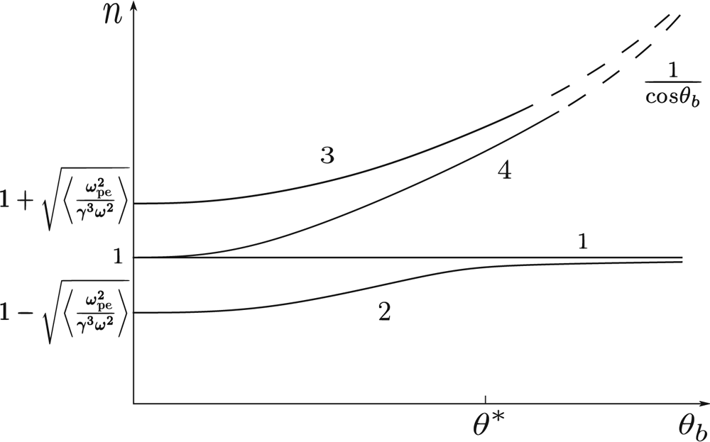
As shown in figure 1, for $A_{p} \gg 1$ the mode $j = 2$ during its propagation transforms from a longitudinal wave for $\theta _{b} \rightarrow 0$ (where $n_{2} < 1$) to a transverse ordinary mode with $n_{2} \approx 1$ for larger angles. We emphasize once again that everywhere below, due to small distances from the neutron star $l \ll R_{L}$ in the analysis of dispersion relations, the angles $\theta _{b}$ , etc. will be assumed to be small.

Figure 1.

Normal modes for $A_{p} \gg 1$ and $a_{p} \ll 1$ with the refractive indices $n \approx 1$ propagating from the neutron star surface as a function of the angle $\theta _{b}$ between the wavevector $\boldsymbol {k}$ and the external magnetic field $\boldsymbol {B}$ (Beskin et al. Reference Beskin, Gurevich and Istomin1988). Waves $j = 1$ (extraordinary X-mode) and $j = 2$ (ordinary O-mode) can escape the pulsar magnetosphere. Subluminal modes $j = 3, 4$ decay at large angles $\theta _{b}$ and cannot escape the pulsar magnetosphere.

Figure 1 shows that the mixing of longitudinal and transverse waves takes place at $\theta _{b} \sim \theta ^{\ast }$, where

(2.13)\begin{equation} \theta^{{\ast}} = \left\langle \frac{\omega_\textrm{pe}^2}{\gamma^{3}\omega^2} \right\rangle^{1/4}.\end{equation}

If for small angles $\theta _{b} < \theta ^{\ast }$, we deal with two transverse modes $n_{1} \approx n_{4} \approx 1$ and with two branches of plasma wave $n_{2,3} \approx 1 \pm a_{p}^{1/2}$, then at large angles $\theta _{b} > \theta ^{\ast }$ we have two transverse modes with $n_{1} \approx n_{2} \approx 1$ and two Alfvén modes with $n_{3} \approx n_{4} \approx 1/\cos \theta _{b}$ propagating along magnetic field lines. As was already noted, these waves are to decay. It should be noted that for cold outflow where $\langle 1/\gamma ^3\rangle \approx \gamma _{s}^{-3}$ we have

(2.14)\begin{equation} A_{p} \approx (\theta^{{\ast}} \gamma_{s})^{4}.\end{equation}

This evaluation is very useful. In particular, rewriting condition $\theta ^{\ast } \gamma _{s} \gg 1$ in the form $\theta ^{\ast } \gg \gamma _{s}^{-1}$, we come to another important conclusion that in the domain where $A_{p} \gg 1$ radiation is generated at the angles $\theta _{b} \ll \theta ^{\ast }$.

As we see, another key parameter of our problem is

(2.15)\begin{align} a_{p} & = \left\langle \frac{\omega_\textrm{pe}^2}{\gamma^{3}\omega^2}\right\rangle\nonumber\\ & \approx 0.56 \times 10^{{-}4} \left(\frac{P}{1 \ \textrm{s}}\right)^{{-}1} \left(\frac{B_{0}}{10^{12}\ \textrm{G}}\right) \left(\frac{\lambda}{10^4}\right) \left(\frac{\gamma_{s}}{100}\right)^{{-}3} \left(\frac{\nu}{1 \ \textrm{GHz}}\right)^{{-}2} \left(\frac{l}{10 R}\right)^{{-}3}. \end{align}

In particular, the mode $j = 2$ cannot propagate outward for $a_{p} > 1$, i.e. for small enough frequencies $\omega$. But for $a_{p} \ll 1$ (and, as was already stressed, only for $A_{p} \gg 1$ in the radiation point), it is this wave that escapes the pulsar magnetosphere and is observed as an ordinary O-mode (see figure 1). For this reason, we consider its properties in detail in § 3.

Once again, we emphasize that the above expressions (2.9)–(2.12) for the refractive indices, $n_{1, 2, 3, 4}$ were obtained under definite restrictions. In addition to condition $A_{p} \gg 1$, it was also assumed that the thermal spread over longitudinal momentum $p = m_{e}cu$ is sufficiently small, so that the averaging over the distribution function $F(u)$ does not cover resonant condition $\omega - k_{\parallel }v_{\parallel } = 0$, i.e.

(2.16)\begin{equation} 1 - n\beta\cos\theta_{b} = 0.\end{equation}

This last circumstance was, in fact, a stumbling block. Indeed, the exact dispersion equation for an infinite magnetic field, but now for arbitrary energy distribution $F(u)$, looks like (Beskin et al. Reference Beskin, Gurevich and Istomin1988; Rafat et al. Reference Rafat, Melrose and Mastrano2019b)

(2.17)\begin{equation} (1-n^2) \left(1-n^2 + (1 - n^2 \cos^2\theta_{b}) \frac{\omega_\textrm{pe}^2}{\omega^2 n \cos\theta_{b}} \int\frac{1}{(1 - n\beta\cos\theta_{b})}\frac{\textrm{d}F}{\textrm{d}u}\,\textrm{d}u\right) = 0.\end{equation}

On the other hand, expressions (2.9)–(2.12) for the refractive indices correspond to the cold plasma approximation, when we can take velocity $v$ out of the integration sign. But in reality, the distribution function of secondary particles $F(u)$ is wide enough (Daugherty & Harding Reference Daugherty and Harding1982; Gurevich & Istomin Reference Gurevich and Istomin1985; Arendt & Eilek Reference Arendt and Eilek2002; Medin & Lai Reference Medin and Lai2010; Timokhin Reference Timokhin2010; Timokhin & Harding Reference Timokhin and Harding2015). Therefore, correction for the superluminal mode $j = 2$ and, all the more, a possibility of the damping for subluminal modes $j = 3, 4$ requires a separate detailed consideration (Rafat et al. Reference Rafat, Melrose and Mastrano2019a,Reference Rafat, Melrose and Mastranob). However, we recall that the damping of subluminal modes itself, which at large angles propagate along the magnetic field and, therefore, cannot leave a neutron star magnetosphere, has never been questioned (Beskin et al. Reference Beskin, Gurevich and Istomin1988).

Obviously, for a quantitative study of thermal effects we must specify the distribution function $F(u)$. As was shown by Arendt & Eilek (Reference Arendt and Eilek2002), the distribution of secondary particles in the plasma rest frame with good accuracy can be approximated by the Jüttner distribution

(2.18)\begin{equation} F^{\prime}(u^{\prime}) = \frac{\exp(-\rho \gamma^{\prime})}{2K_{1}(\rho)},\end{equation}

with parameter $\rho = m_{e} c^2/T \approx 1$. Here $K_{1}$ is the Macdonald function of order one. This implies relativistic temperature $T \approx m_{e}c^2$. Accordingly, in the laboratory (neutron star) reference frame we have

(2.19)\begin{equation} F(u) = \frac{\exp[-\rho \gamma_{s}\gamma(1 - \beta\beta_{s})]}{2K_{1}(\rho)}\gamma_{s}(1 - \beta\beta_{s}).\end{equation}

Note that, in contrast to Rafat et al. (Reference Rafat, Melrose and Mastrano2019b), we consider normalization $\int F(u)\,\textrm {d}u = 1$. However, below we consider a wider class of distribution functions $F(u)$, since the distribution function (2.19) does not always adequately describe the distribution of secondary particles outflowing from the magnetosphere of a neutron star.

Thus, the goal of our study is to clarify how the thermal effects affect the propagation properties of radio waves in the pulsar magnetosphere. Therefore, in contrast to the works of Rafat et al. (Reference Rafat, Melrose and Mastrano2019a) and Rafat et al. (Reference Rafat, Melrose and Mastrano2019b), our main task is to analyse the dependence of their refractive indices $n$ on the angle $\theta _{b}$. It is clear that in the infinite magnetic field approximation (2.17) considered here, the extraordinary X-mode $j = 1$ remains unchanged. Indeed, as the electric vector of this wave is perpendicular to the external magnetic field, this mode cannot interact with plasma particles. As a result, we have $n_{1} = 1$, i.e. this mode propagates rectilinearly in the pulsar magnetosphere. For this reason, we discuss only three other modes.

3. Superluminal O-mode

At first, let us consider the O-mode $j = 2$; remember that here we consider the case $A_{p} \gg 1$. As shown in figure 1, for this wave $n_{2} < 1$, i.e. it is a superluminal mode. Using the standard Lorentz transformation to the plasma rest frame

(3.1)\begin{equation} n^{\prime}\cos\theta_{b}^{\prime} = \frac{n\cos\theta_{b} - \beta_{s}}{1 - n\beta_{s}\cos\theta_{b}}, \end{equation}

we obtain for $\gamma _{s} \gg 1$, $A_{p} \gg 1$, and $\theta _{b} = 0$,

(3.2)\begin{equation} n_{2}^{\prime} \approx{-}1 + \frac{1}{(1-n_{2})\gamma_{s}^2} \approx{-}1 + A_{p}^{{-}1/2}.\end{equation}

As $\omega ^{\prime } = \gamma _{s}\omega (1 - n_{2}\beta ) > 0$, one can conclude that for $\theta _{b} = 0$ in the plasma rest frame the O-mode $j = 2$ corresponds to superluminal branch of a plasma wave propagating to the star surface.

On the other hand, as for the superluminal O-mode, the denominator in (2.17) is positive for all particle four-velocities $u$, one can obtain using integrating by parts,

(3.3)\begin{equation} 1 - n_{2}^2 - (1 - n_{2}^2 \cos^2\theta_{b}) \frac{\omega_\textrm{pe}^2}{\omega^2 } \left\langle \frac{1}{\gamma^3(1 - n_{2}\beta\cos\theta_{b})^2}\right\rangle = 0.\end{equation}

For cold plasma (and for $|n - 1| \gg |\beta - 1|$, which is just true for $A_{p} \gg 1$) one can put $\beta = 1$, and we return to (2.10). On the other hand, for a wide enough distribution function, i.e. for parameter $\rho \sim 1$ incoming into the Jüttner distribution function (2.18), the value of $\beta$ under the integral sign cannot be considered constant, and therefore a more detailed study is required.

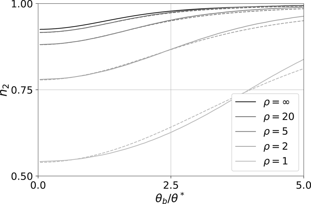
Figure 2 shows how the refractive index $n_{2}$ depends on the angle $\theta _{b}$ for $A_{p} \gg 1$ for different parameters $\rho$ (solid lines). The dashed lines correspond to the simplified expression (2.10) used by Beskin et al. (Reference Beskin, Gurevich and Istomin1988), where during the integration on $\textrm {d}u$ in (2.17) the condition $\beta = 1$ was assumed.

Figure 2.

Dependence of refractive index $n_{2}$ on the angle $\theta _{b}$ for different parameters $\rho = m_{e} c^2/T$ for $\gamma _{s} = 100$, $\lambda = 10^{4}$, $P = 1$ s, $B = 10^{11}$ G and $\nu = 1$ GHz ($A_{p} \sim 10^{6}$). The solid lines correspond to numerical solution of (3.3) and the dashed lines correspond to analytical expression (2.10) for different parameters $\rho$.

As we see, for $\rho \sim 1$ the difference in the refractive index from unity is already three to four times larger than that for cold plasma. It should be also emphasized that even for hot enough plasma (i.e. for $\rho \sim 1$) the simplified evaluation (2.10) reproduces a good enough dependence of the refractive index $n_{2}$ on angle $\theta _{b}$. Note that in this figure, the angle $\theta _{b}$ is expressed in terms of $\theta ^{\ast }$, which is different for different frequencies $\omega$.

Remember that it is the wave $j = 2$ that escapes from the pulsar magnetosphere as the ordinary O-mode (Barnard & Arons Reference Barnard and Arons1986; Beskin & Philippov Reference Beskin and Philippov2012). In this case, the difference in the refractive index from unity leads to a deviation of the wave from the magnetic axis. As a result, the mean profile formed by the O-mode turns out to be wider than for the extraordinary X-mode $j = 1$.

To obtain the width of the directivity pattern $W_{r}$, we must now determine the propagation path of the O-mode. As was shown by Beskin et al. (Reference Beskin, Gurevich and Istomin1988), for small angles $\theta _{\perp } = k_{\perp }/k \ll 1$ and $\alpha = (3/2)r_{\perp }/l \ll 1$ where $\alpha$ is the angle between the magnetic field and the magnetic axis, and $r_{\perp }$ and $k_{\perp }$ are the components of the vectors perpendicular to the magnetic axis, in dipole magnetic field the equations of geometric optics $\textrm {d}\boldsymbol {r}/\textrm {d} t = \partial \omega /\partial \boldsymbol {k}$, $\textrm {d}\boldsymbol {k}/\textrm {d} t = -\partial \omega /\partial \boldsymbol {r}$ are reduced to the following system:

(3.4)\begin{gather} \frac{\textrm{d}r_{{\perp}}}{\textrm{d} l} = \frac{\theta_{{\perp}}}{n} - \frac{1}{n^2} \frac{\partial n}{\partial \theta_{b}}, \end{gather}

(3.5)\begin{gather}\frac{\textrm{d}\theta_{{\perp}}}{\textrm{d} l} = \frac{3}{2} \frac{1}{n^2 l} \frac{\partial n}{\partial \theta_{b}}. \end{gather}

Here $l$ is the distance from the star centre, and we use relations $\theta _{b} = \alpha - \theta _{\perp }$ and $\textrm {d}l/\textrm {d}t = c$.

Differentiating now the second bracket in the dispersion equation (2.17) with respect to $\theta _{b}$, we obtain for the derivative $\partial n_{2}/\partial \theta _{b}$,

(3.6)\begin{equation} \frac{\partial n_{2}}{\partial \theta_{b}} = \theta_{b}\frac{A}{1 + A}, \end{equation}

where

(3.7)\begin{equation} A = 4\frac{\omega_\textrm{pe}^2}{\omega^2} \left\langle \frac{u(2u^2\xi-1)}{(2u^2\xi+1)^3}\right\rangle \end{equation}

and $\xi = 1 - n_{2} - \theta _{b}^2/2$ is to be the root of the dispersion equation

(3.8)\begin{equation} \xi - \frac{\theta_{b}^2}{2} = 4\frac{\omega_\textrm{pe}^2}{\omega^2} \left\langle \frac{u\xi}{(2u^2\xi+1)^2}\right\rangle . \end{equation}

As was already mentioned, we present all the expressions in the limit of $\theta _{b} \ll 1$ and $|n - 1| \ll 1$.

In the limit $u^2\xi \gg 1$ we reduce to ‘hydrodynamical’ relations

(3.9)\begin{gather} \frac{\textrm{d}r_{{\perp}}}{\textrm{d} l} = \theta_{{\perp}} + \frac{(\alpha - \theta_{{\perp}})}{2} \left[1-\frac{(\alpha - \theta_{{\perp}})^2}{[16 a_{p}(l) +(\alpha - \theta_{{\perp}})^4]^{1/2}} \right], \end{gather}

(3.10)\begin{gather}\frac{\textrm{d}\theta_{{\perp}}}{\textrm{d} l} = \frac{3}{4} \frac{(\alpha - \theta_{{\perp}})}{l} \left[1-\frac{(\alpha - \theta_{{\perp}})^2}{[16 a_{p}(l) +(\alpha - \theta_{{\perp}})^4]^{1/2}} \right], \end{gather}

obtained by Beskin et al. (Reference Beskin, Gurevich and Istomin1988). Here $a_{p}$ is given by relation (2.15) and $n_{2}$ is to be found as a solution of (3.3). Note that during integration it is necessary to take into account the dependence of $a_{p} = \langle \omega _\textrm {pe}^2/(\gamma ^3\omega ^2)\rangle$ via $\omega _\textrm {pe}$ on $l$ (figure 2 shows the dependence of the refractive index $n_{2}$ on the angle $\theta _{b}$ at a given point, not along the beam propagation). As a result, integrating the system of (3.4) and (3.5), we obtain for the width of the directivity pattern

(3.11)\begin{equation} W_{r} = 2 \theta_{{\perp}}(\infty).\end{equation}

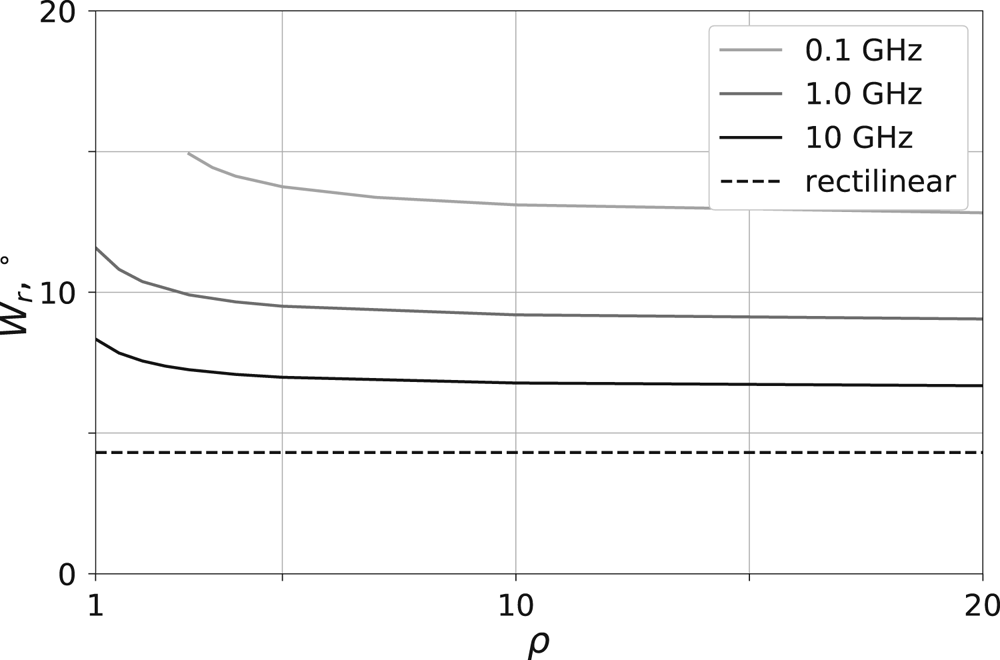
The dependence of the width of the directivity pattern $W_{r}$ (3.11) on parameter $\rho$ is shown in figure 3 for the same parameters as in figure 2; we start at the point $l= 3 R$, where $\theta _{\perp } = \alpha$ (radiation along the magnetic field line). The dashed line corresponds to rectilinear propagation when $W_{r} = 2 \, \alpha (3 R)$. As we see, thermal effects do not significantly affect the width of the directivity pattern.

Figure 3.

Dependence of the width of the directivity pattern $W_{r}$ (3.11) (in degrees) on parameter $\rho = m_{e} c^2/T$ for $\gamma _{s} = 100$, $\lambda = 10^{4}$, $P = 1$ s, magnetic field on the star surface $B_{0} = 10^{12}$ G and for starting point $l=3 R$. The dashed line corresponds to rectilinear propagation.

A detailed study of the effects of the refraction of an ordinary wave on the formation of mean profiles of radio pulsars will be carried out in a separate work. At the same time, it should be emphasized that the starting radius $l = 3 R$ used in this work was selected taking into account the observational data. Indeed, according to the statistical analysis performed by Rankin (Reference Rankin1990) and Maciesiak, Gil & Melikidze (Reference Maciesiak, Gil and Melikidze2012), the intrinsic pulse width $W_{r}$ for the core component (just corresponding to X-mode in our classification) is equal to $W_{r} = W_{0}/P^{1/2}$, where $W_{0} = 2^{\circ }$–$3^{\circ }$. Assuming that this value corresponds to the opening magnetic field lines $3 (\varOmega l/c)^{1/2}$ at the distance $l$, we obtain for the height of the radio emission $l \sim 3$ stellar radius. As for the cases when the observed pulse width turns out to be larger than these values (see, for example, Mitra Reference Mitra2017), this, as is well known, can be associated either with non-orthogonality (when the observable pulse width $W_\textrm {obs} = W_{r}/\sin \chi$) or with the fact that the average profile is determined by the O-mode $j = 2$. We can note that under the condition $\rho \gg 1$, the dependence of the window width $W_{r}$ on the frequency $\nu$ shown in figure 2 with good accuracy satisfies the dependence

(3.12)\begin{equation} W_{r} \approx 8^{{\circ}} \left(\frac{\nu}{1 \ \textrm{GHz}}\right)^{{-}0.14} \left(\frac{P}{1 \ \textrm{s}}\right)^{{-}0.43} \left(\frac{B_{0}}{10^{12}\ \textrm{G}}\right)^{0.07} \left(\frac{\gamma_{s}}{100}\right)^{{-}0.11} \left(\frac{\lambda}{10^{4}}\right)^{0.07} \left(\frac{l}{3 R}\right)^{0.15}, \end{equation}

predicted by Beskin et al. (Reference Beskin, Gurevich and Istomin1988) for an O-mode for $P = 1$ s, $\lambda = 10^4$ and $l = 3 R$. For more realistic temperatures $\rho \sim 1$, the pulse width is to be even larger.

In conclusion, we note that, according to relation (2.7), for frequencies $\nu = \omega /2{\rm \pi} \sim 1$ GHz in the region of radio emission generation $l < 100 R$ ($A_{p} > 1$), the refractive index $n_{2}$ (2.10) differs significantly from unity. On the other hand, as was shown by Rafat et al. (Reference Rafat, Melrose and Mastrano2019a), mode crossing occurs only if the refractive index $n$ is close to unity (in the plasma rest frame $|n^2-1| \sim \omega _\textrm {pe}^2/\omega _{B}^2$). Hence, such an intersection of modes is possible only in an insignificant range of heights $l \sim 100 R$ ($A_{p} \sim 1)$, when in the hydrodynamic limit one should use the more accurate expression

(3.13)\begin{equation} n_{2} \approx 1 + \frac{1}{2\gamma_{s}^2} - \left(\frac{\omega_\textrm{pe}^2}{\gamma_{s}^3\omega^2}\right)^{1/2} , \end{equation}

giving the possibility of fulfilling the condition $n_{2} \approx 1$. On the other hand, at the distances $l \sim 10 R$ such crossing takes place for frequencies $\nu > 100$ GHz only.

Thus, for frequencies $\nu \sim 1$ GHz the mode crossing cannot take place for the O-mode in the generation region. As far as the heights $l \sim 100 R$, the O-mode passes this region at much higher angles $\theta _{b} \gg \theta _\textrm {cr}$. Therefore, for the O-mode $j = 2$ emitted in the region $l \ll 100 R$ the influence of thermal effects in the region of mode crossing can be neglected.

4. Subluminal plasma-Alfvén mode

Now, let us consider mixing plasma-Alfvén mode $j = 3$ ($n_{3} > 1$, see figure 1); again, we consider the case $A_{p} \gg 1$. For this mode for $\theta _{b} = 0$ we have

(4.1)\begin{equation} n_{3}^{\prime} \approx{-}1 + \frac{1}{(1-n_{3})\gamma_{s}^2} \approx{-}1 - A_{p}^{{-}1/2} \end{equation}

and $\omega ^{\prime } = \gamma _{s}\omega (1 - n_{2}\beta ) < 0$. Thus, for $\theta _{b} = 0$ in the plasma rest frame this mode corresponds to the subluminal branch of a plasma wave also propagating to the star's surface. On the other hand, for large enough angles $\theta _{b}$ in the laboratory frame, (2.11) gives $n_{3} \approx 1 + \theta _{b}^2/2 \approx 1/\cos \theta _{b}$. This dispersion equation corresponds to an Alfvén mode propagating along the magnetic field line.

It is clear that the main difference between the subluminal ($\,j = 3$) and the superluminal ($\,j = 2$) wave is that it becomes possible to perform the Cherenkov resonance condition (2.16). In this case, since we consider the problem of wave propagation in a curved external magnetic field when the angle $\theta _{b}$ changes along the propagation path, the resonance condition is to be fulfilled even for cold plasma. That is why in figure 1 it is the angle $\theta _{b}$ that is chosen as the main parameter.

However, for cold plasma, the resonance condition (2.16) occurs for the angles $\theta _{b}$ larger than the angle $\theta ^{\ast }$. This result can be obtained immediately if we write down the resonance condition in the form $(n - 1) - 1/2\gamma ^2 - \theta _{b}^2/2 = 0$. For $n_{3} > 1 + (\omega _\textrm {pe}^2/\gamma ^3\omega ^2)^{1/2}$ and for $A_{p } \gg 1$ we just obtain $\theta _\textrm {res} > \theta ^{\ast }$. Therefore, we can conclude that for cold plasma, the damping of the plasma-Alfvén mode occurs only for large enough angles $\theta _{b}$ (as shown in figure 1).

On the other hand, for a fairly wide distribution function $F(u)$, i.e. for $\rho > 1$, there are particles which are in resonance with the wave even for $\theta _{b} = 0$. For ultrarelativistic plasma ($\gamma _{s} \gg 1$) and for small angles $\theta _{b} \ll \theta ^{\ast }$, the resonance condition can be written in the form $\gamma _\textrm {res} \approx 1/\theta ^{\ast }$. As a result, using relation (2.14), we obtain for the exponent $a(\gamma _\textrm {res}) = \rho \gamma _{s} \gamma _\textrm {res} (1 - \beta _{s} \beta _\textrm {res})$ in the Jüttner distribution $F(u) \propto \exp (-a)$ for resonance particles:

(4.2)\begin{equation} a(\gamma_\textrm{res}) \approx \rho \gamma_{s}\theta^{{\ast}} \sim \rho A_{p}^{1/4}. \end{equation}

Thus, for $A_{p} \gg 1$ the damping of the plasma-Alfvén mode for $\theta _{b} = 0$ is to be weak even for $\rho \sim 1$.

To determine the attenuation of the wave $j = 3$ for an arbitrary temperature, it is convenient to find the solution of the dispersion equation (2.17) in the form

(4.3)\begin{equation} n_{3}\cos\theta_{b} = 1 + x_{3}.\end{equation}

Then for small angles $\theta _{b} \ll 1$, relativistic energies ($\beta \approx 1 - 1/(2u^2)$) and for $x_{3} \ll 1$, we obtain

(4.4)\begin{equation} x_{3}\left(x_{3} + \frac{\theta_{b}^2}{2}\right) = I_{3}(x_{3}),\end{equation}

where

(4.5)\begin{equation} I_{3}(x_{3}) = \frac{\omega_\textrm{pe}^2}{\omega^2(1+x_{3})} \left[ \left.{\int\kern-10pt} \frac{2u^2 x_{3}^2}{(2u^2 x_{3} - 1)} \frac{\textrm{d}F}{\textrm{d}u} \, \textrm{d}u + \mathrm{i}{\rm \pi} \frac{x_{3}^{1/2}}{2\sqrt{2}} \frac{\textrm{d}F}{\textrm{d}u}\right|_{u = (2x_{3})^{{-}1/2}}\right]. \end{equation}

Here, as usual, for small imaginary part $\textrm {Im}\, n$ in comparison with its real part, the real part of the integral ${\int\kern-10pt}$ is to be taken in the sense of the principal value.

Besides, for small angles $\theta _{b} \ll \theta ^{\ast }$, when according to (2.11) $n_{3} \approx 1 + a_{p}^{1/2}$, our definition (4.3) gives $x_{3} \approx a_{p}^{1/2}$. This evaluation can be easily obtained from condition $x_{3} \approx I_{3}^{1/2}$ resulting from (4.4), if we neglect the second term in (4.5) and use the limit $x_{3} u^2 \gg 1$. The last relation results from evaluation $x_{3} u^2 \sim a_{p}^{1/2}\gamma _{s}^2 \sim A_{p}^{1/2}$. In particular, this implies that the resonant particles correspond to the low-energy part of the distribution function ($\gamma _\textrm {res} \ll \gamma _{s}$). As a result, expanding the denominator in (4.5) by a small parameter $1/(2 u^2 x_{3})$, we obtain that $I_{3} = J_{3}$, where

(4.6)\begin{equation} J_{3}(x_{3}) = \frac{\omega_\textrm{pe}^2}{\omega^2(1+x_{3})} {\int\kern-10pt} x_{3} \left(1+\frac{1}{2 u^2 x_{3}}\right) \frac{\textrm{d}F}{\textrm{d}u} \, \textrm{d}u \approx \left\langle \frac{\omega_\textrm{pe}^2}{\gamma^3 \omega^2}\right\rangle ,\end{equation}

as the first integration term vanishes due to the identity $\int (\textrm {d}F/\textrm {d}u) \, \textrm {d}u = 0$.

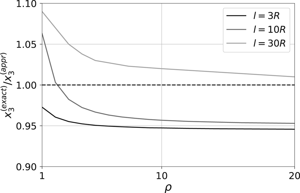
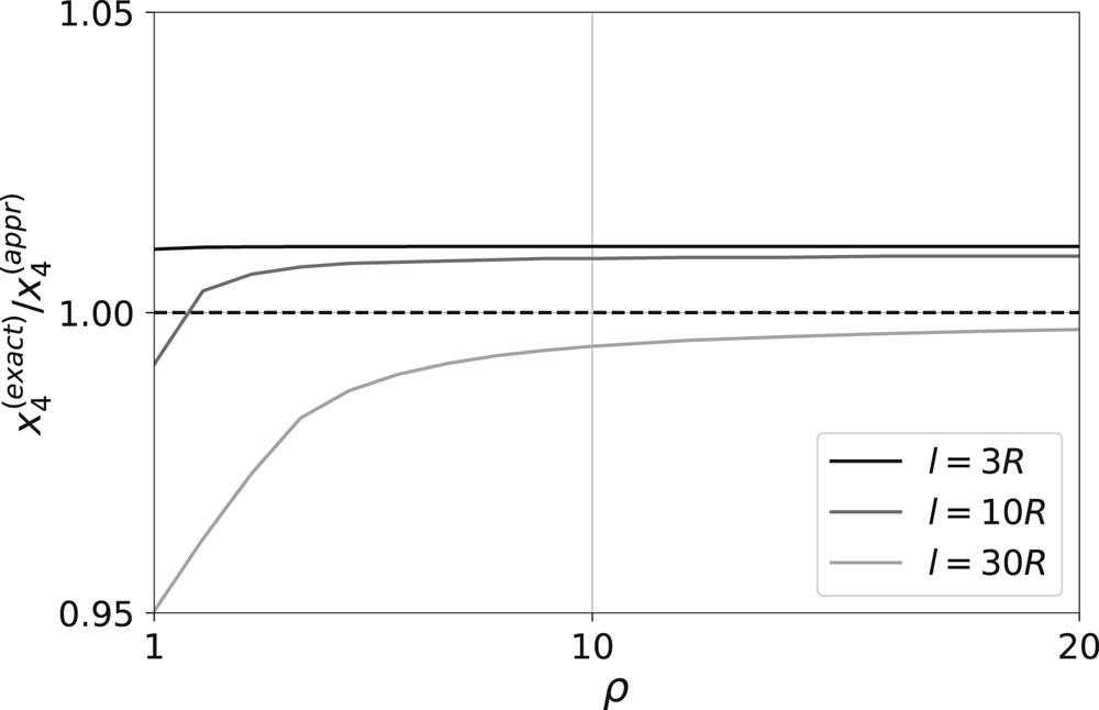
Here it is interesting to check the accuracy of the approximation under consideration. For this, in figure 4 we show a comparison of the ratios of the values $x_{3}$ obtained from relations (4.4) and (4.6) and from exact dispersion equation (2.17) for $\theta _{b} = 0$, $\lambda = 10^4$ and $\nu = 1$ GHz. As we see, a good enough agreement does exist for different starting points $l$.

Figure 4.

Comparison of the ratio of values $x_{3}^{(\textrm {exact})}/x_{3}^{(\textrm {appr})}$ obtained from relations (4.4) and (4.6) and from exact dispersion equation (2.17) for different starting points.

We also note that there are no contradictions with the results presented by Rafat et al. (Reference Rafat, Melrose and Mastrano2019b), since the range of parameters we are considering (precisely due to condition $A_{p} > 1$) corresponds to the values $0 < \textrm {log}_{10}\gamma _{\phi }^{\prime } < 2$ (for $\gamma _{s} = 100$) where, according to their figure 11, the results actually match each other. Wherein, the accuracy of the approximation becomes worse as $A_{p} \rightarrow 1$ ($\gamma _{\phi }^{\prime } \rightarrow \gamma _{s}$).

Further, one can see that the leading (real) term in $I_{3}$ actually does not depend on $x$. Therefore, for weak damping, the imaginary part of $n_{3} \approx 1 + x_{3} + \theta _{b}^2/2$ is completely determined by the second term,

(4.7)\begin{equation} \textrm{Im} \, n_{3} = \left.\frac{\rm \pi}{2\sqrt{2}} \frac{\omega_\textrm{pe}^2}{\omega^2} \frac{[(16 J_{3} + \theta_{b}^4)^{1/2} - \theta_{b}^2]^{1/2}}{(16 J_{3} + \theta_{b}^4)^{1/2}} \frac{\textrm{d}F}{\textrm{d}u}\right|_{u = (2x_{3})^{{-}1/2}},\end{equation}

since the resonance condition is achieved in the low-energy region, where $\textrm {d}F/\textrm {d} u > 0$. Nevertheless, $\textrm {Im}\, n_{3} > 0$, which corresponds to the attenuation of the wave $j = 3$. This is due to the fact that the wave frequency is negative in the plasma rest reference frame (see appendix A for more detail).

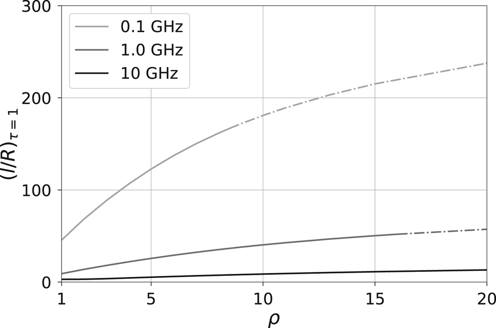
Figure 5 shows the levels $l = r_{d}$ at which the optical depth, for the mode $j = 3$,

(4.8)\begin{equation} \tau = \frac{\omega}{c} \int_{l=r_{0}}^{l=r_{d}} \textrm{Im} \, n_{3}\,\textrm{d}l,\end{equation}

becomes equal to unity. Integration was carried out using general relations (3.4)–(3.5) resulting in (Beskin et al. Reference Beskin, Gurevich and Istomin1988)

(4.9)\begin{gather} \frac{\textrm{d}r_{{\perp}}}{\textrm{d} l} = \theta_{{\perp}} + \frac{(\alpha - \theta_{{\perp}})}{2} \left[1 + \frac{(\alpha - \theta_{{\perp}})^2}{[16 a_{p}(l) +(\alpha - \theta_{{\perp}})^4]^{1/2}} \right], \end{gather}

(4.10)\begin{gather}\frac{\textrm{d}\theta_{{\perp}}}{\textrm{d} l} = \frac{3}{4} \frac{(\alpha - \theta_{{\perp}})}{l} \left[1 + \frac{(\alpha - \theta_{{\perp}})^2}{[16 a_{p}(l) +(\alpha - \theta_{{\perp}})^4]^{1/2}} \right]. \end{gather}

As in all the previous figures, we set the radiation radius to $r_{0} = 3 R$. The solid lines correspond to the ratio $\theta _{b}/\theta ^{\ast } < 1$ at the level $\tau = 1$, and the dashed-dotted lines correspond to the ratio $\theta _{b}/\theta ^{\ast } > 1$.

Figure 5.

Levels $l = r_{d}$ at which the optical depth $\tau$ (4.8) for mode $j = 3$ becomes equal to one for the same parameters as in figure 3. The solid lines correspond to the ratio $\theta _{b}/\theta ^{\ast } < 1$ at the level $\tau = 1$ and the dashed-dotted lines correspond to the ratio $\theta _{b}/\theta ^{\ast } > 1$.

As we can see, even for $\rho = 1$ the wave damps at the heights significantly higher than the radiation level. Therefore, there is no doubt in the very existence of this wave. On the other hand, for $\rho \sim 1$ the damping occurs at the angles $\theta _{b}$ even smaller than local $\theta ^{\ast }(l)$, so that the inclusion of thermal effects into consideration leads to the fact that this wave attenuates at much smaller distances from a neutron star in comparison with the case of cold plasma.

5. Subluminal Alfvén mode

Finally, let us consider the Alfvén mode $j = 4$. For $\theta _{b} = 0$ it corresponds to the transverse ordinary O-mode ($n_{4} = 1$), but for large enough $\theta _{b}$ (and again for $A_{p} \gg 1$) we obtain $n_{4} \approx 1/\cos \theta _{b}$, i.e. this mode also propagates along the magnetic field line. Unlike the mode $j = 3$, for the mode $j = 4$ the resonance condition cannot be satisfied for $\theta _{b} = 0$. However, it becomes possible for $\theta _{b} > 0$, the resonant particles having the energies much larger than the average energy of outflowing plasma ($\gamma _\textrm {res} \gg \gamma _{s}$).

Due to (2.12), for this mode it is also convenient to find the solution of the dispersion equation (2.17) in the form

(5.1)\begin{equation} n_{4}\cos\theta_{b} = 1 + x_{4}.\end{equation}

Then for small angles $\theta _{b} \ll 1$ and relativistic energies ($\beta \approx 1 - 1/(2u^2)$), we obtain

(5.2)\begin{equation} x_{4} = \frac{\theta_{b}^2/2}{I_{4}(x_{4}) - 1},\end{equation}

where

(5.3)\begin{equation} I_{4}(x_{4}) ={-} \frac{\omega_\textrm{pe}^2}{\omega^2} \left[ \left.{\int\kern-10pt} \frac{2u^2}{1 - 2 u^2 x_{4}} \frac{\textrm{d}F}{\textrm{d}u} \, \textrm{d}u - \mathrm{i} {\rm \pi} \frac{x_{4}^{{-}3/2}}{2\sqrt{2}} \frac{\textrm{d}F}{\textrm{d}u}\right|_{u = (2x_{4})^{{-}1/2}}\right]. \end{equation}

Here, in contrast to (4.5), for the Alfvén mode $j = 4$ we have $x_{4}u^2 \ll 1$. Indeed, neglecting $2 u^2 x_{4}$ in the denominator and the second term in (5.3), we obtain for small angles $\theta _{b}$

(5.4)\begin{equation} x_{4} = \frac{\theta_{b}^2/2}{J_{4} - 1},\end{equation}

where

(5.5)\begin{equation} J_{4} = 4 \frac{\omega_\textrm{pe}^2\langle u\rangle }{\omega^2} \approx 4 A_{p}. \end{equation}

As a result, we obtain $x_{4}u^2 \sim \gamma _{s}^2\theta _{b}^2/A_{p}$, so that up to the angles $\theta _{b} \sim \theta ^{\ast }$ we have $x_{4}u^2 < A_{p}^{-1/2}$ due to (2.14).

Figure 6 shows a comparison of the ratios of the values $x_{4}$ obtained from relations (5.4) and from exact dispersion equation (2.17) for $\theta _{b} = 0.02$, $\lambda = 10^4$ and $\nu = 1$ GHz. As we see, a good agreement exists for different starting points $l$ for Alfvén wave $j = 4$ as well. In particular, such a good agreement also shows that the corresponding root of the dispersion equation is far enough from the value $n = 1/\cos \theta _{b}$. Thus, the contradiction with the paper by Rafat et al. (Reference Rafat, Melrose and Mastrano2019b) is removed, where it was pointed out that the approach under consideration is not applicable for $n \approx 1/ \cos \theta _{b}$.

Figure 6.

Comparison of the ratio of values $x_{4}^{(\textrm {exact})}/x_{4}^{(\textrm {appr})}$ obtained from relations (5.4)–(5.5) and from exact dispersion equation (2.17) for different starting points.

Further, as $I_{4}(0) \approx 4 A_{p}$, we can conclude that for $A_{p} \gg 1$ the disturbance $x_{4}$ to expression $n_{4}$ (2.12) is indeed small, with resonant particles being absent for $\theta _{b} = 0$. Certainly, as previously mentioned, this expression can only be used if the second term in brackets in (5.3) is much smaller than the first term. As was already highlighted, this implies that for this mode the resonant particles correspond to the high-energy part of the distribution function.

Finally, we see that the leading (real) term in $J_{4}$ again does not depend on our variable $x_{4}$. Therefore, for weak damping, the imaginary part of $n_{4} \approx 1 + x_{4} + \theta _{b}^2/2$ is completely determined by the second term

(5.6)\begin{equation} \textrm{Im} \, n_{4} ={-}\frac{\rm \pi}{8} \left. \frac{J_{4}^{1/2}}{\langle u\rangle \theta_{b}} \frac{\textrm{d}F}{\textrm{d}u}\right|_{u = (2x_{4})^{{-}1/2}}.\end{equation}

Here we neglect the terms of the order of $A_{p}^{-1/2}$. Since now the resonance condition is achieved in the high-energy region, where $\textrm {d}F/\textrm {d} u < 0$, we again have $\textrm {Im}\, n_{4} > 0$ corresponding to attenuation of the wave $j = 4$.

Note that, in reality, the relation (5.2) has no singularity. Indeed, expanding $I_{4}$ as

(5.7)\begin{equation} I_{4}(x_{4}) ={-} \frac{\omega_\textrm{pe}^2}{\omega^2} {\int\kern-10pt} 2u^2(1 + 2 u^2 x_{4}) \frac{\textrm{d}F}{\textrm{d}u} \ \textrm{d}u \approx 4 \frac{\omega_\textrm{pe}^2\langle u\rangle }{\omega^2} + 16 \frac{\omega_\textrm{pe}^2\langle u^3\rangle }{\omega^2}x_{4} + \cdots \end{equation}

and assuming that $\omega _\textrm {pe}^2\langle u^3\rangle /\omega ^2 \approx J_{4}\gamma _{s}^2$ we obtain

(5.8)\begin{equation} x_{4} \approx \frac{-(J_{4} - 1) \pm [(J_{4} - 1)^2 + 8\,J_{4}\gamma_{s}^2\theta_{b}^2]^{1/2}}{8\,J_{4}\gamma_{s}^2}, \end{equation}

where the ‘plus’ sign corresponds to $J_{4} > 1$, and the ‘minus’ sign to $J_{4} < 1$. As a result, $n_{4}(\theta _{b})$ always remains larger than unity if $J_{4} > 1$ and vice versa. Thus, during the propagation the wave $j = 4$ never achieves the singularity $x_{4} = 0$ (i.e. $n_{4} \cos \theta _{b} = 0$), noted by Rafat et al. (Reference Rafat, Melrose and Mastrano2019b). On the other hand, for $A_{p} \ll 1$ ($I_{4} \ll 1$) expression (5.2) results in

(5.9)\begin{equation} n_{4} \approx 1 - 2\frac{\omega_\textrm{pe}^2\langle u\rangle }{\omega^2} \theta_{b}^2,\end{equation}

which is in agreement with Beskin et al. (Reference Beskin, Gurevich and Istomin1988) and Rafat et al. (Reference Rafat, Melrose and Mastrano2019b).

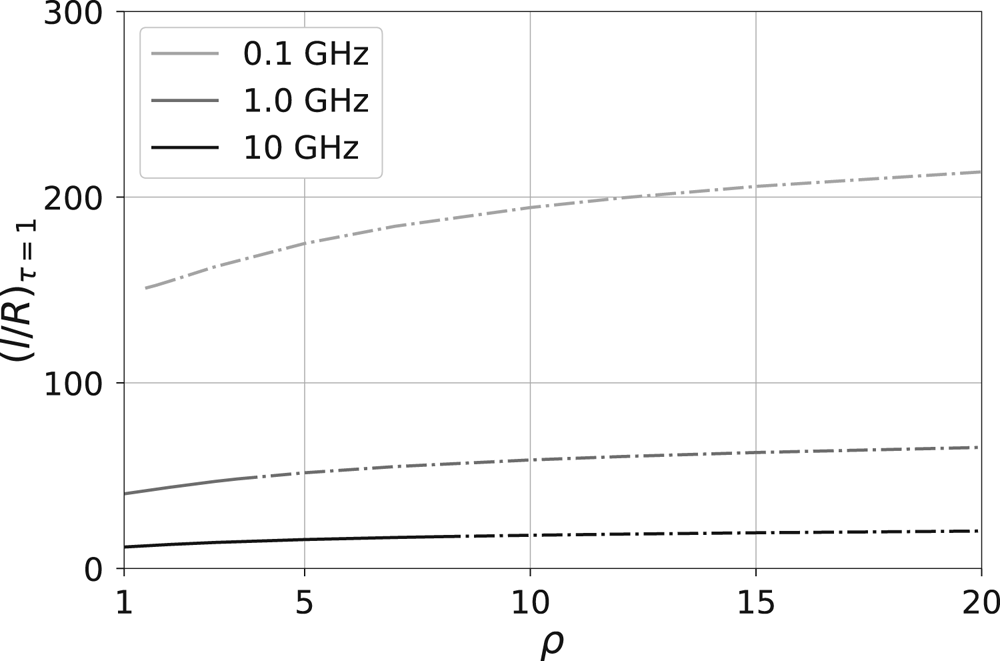
Figure 7 shows the levels $l = r_{d}$ at which the optical depth $\tau$ becomes equal to unity for the mode $j = 4$. Integration was carried out using general relations (3.4)–(3.5) resulting in

(5.10)\begin{gather} \frac{\textrm{d}r_{{\perp}}}{\textrm{d} l} = \alpha, \end{gather}

(5.11)\begin{gather}\frac{\textrm{d}\theta_{{\perp}}}{\textrm{d} l} = \frac{3}{2} \frac{\theta_{b}}{l}. \end{gather}

Figure 7.

Same as in figure 5 for the Alfvén mode $j = 4$.

As previously mentioned, we set the radiation radius to $r_{0} = 3 R$. The solid lines correspond to the ratio $\theta _{b}/\theta ^{\ast } < 1$ at the level $\tau = 1$ and the dashed-dotted lines correspond to the ratio $\theta _{b}/\theta ^{\ast } > 1$. As we see, thermal effects for the Alfvén wave $j = 4$, in general, are the same as for the wave $j = 3$. Again, even for $\rho = 1$ the wave damps at the heights significantly higher than the radiation level. On the other hand, for $\rho \sim 1$ the damping can occur at angles $\theta _{b}$ even smaller than local transition angle $\theta ^{\ast }(l)$. The characteristic values for concentration $N_{e}$ turn out to be four orders of magnitude lower than those for ordinary pulsars. As can be seen from relations (2.7) and (2.15), the values of $A_{p}$ and $a_{p}$ should be smaller in the same proportion.

6. Alternative distribution function

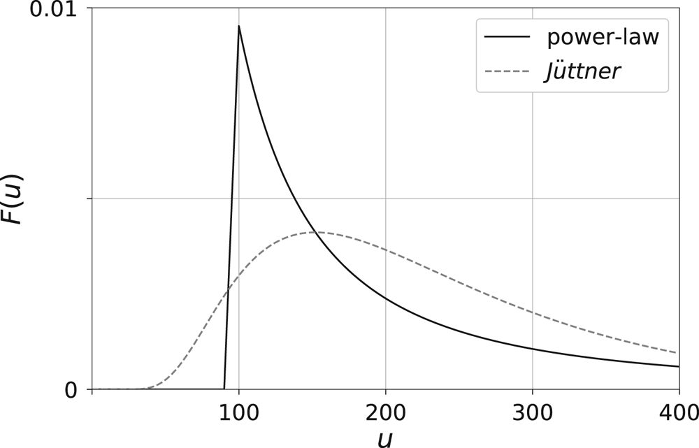
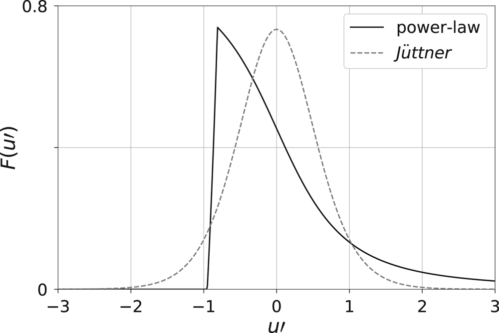
As was already stated, the Jüttner distribution function (2.19) may not accurately describe the real distribution function of particles flowing along open magnetic field lines in the pulsar magnetosphere. Here we rely on the results obtained under the analysis of processes of secondary electron–positron plasma generation in the polar magnetosphere of radio pulsars obtained by Gurevich & Istomin (Reference Gurevich and Istomin1985). For this reason, we consider another particle distribution function in the laboratory frame (see figures 8 and 9):

(6.1)\begin{equation} F(u) = \left\{ \begin{array}{@{}ll} 0, & u < u_0-\varDelta, \\ \dfrac{u-u_0+\varDelta}{\varDelta(u_0+\varDelta/2)}, & u_0-\varDelta < u < u_0, \\ \dfrac{u_0^2}{(u_0+\varDelta/2)} u^{{-}2}, & u > u_0. \end{array} \right. \end{equation}

Accordingly, the derivative of the distribution function over $u$ is

(6.2)\begin{equation} \frac{\textrm{d}F(u)}{\textrm{d}u} = \left\{ \begin{array}{@{}ll} 0, & u < u_0-\varDelta, \\ \dfrac{1}{\varDelta(u_0+\varDelta/2)}, & u_0-\varDelta < u < u_0, \\ -\dfrac{2u_0^2}{(u_0+\varDelta/2)} u^{{-}3}, & u>u_0. \end{array} \right. \end{equation}

In addition, we will discuss in more detail the dispersion properties of the waves propagating in the pulsar magnetosphere, and we will not limit ourselves to small angles $\theta _{b} \ll 1$.

Figure 8.

Particle distribution function $F(u)$ (6.1) in the laboratory frame, $u_0=100, \varDelta =10$. The dashed curve represents the Jüttner function with $\rho =4$ in the frame moving with the Lorentz factor $\gamma _s=210$.

Figure 9.

Particle distribution function $F(u')$ (6.1) in the rest frame, where the mean velocity is equal to zero. The Lorentz factor of motion of this frame is $\gamma _s = 210$. The dashed line shows the Jüttner function (2.18) with $\rho =4$.

First, let us make some remarks regarding the choice of an alternative distribution function $F(u)$ (6.1). It is clear that the particle distribution function in the magnetosphere in the laboratory frame is a streaming function, i.e. there are no particles with negative momentum $u$. In addition, the cascade production of electrons and positrons from high to low energies ends even at rather high momenta, $u \simeq 10^{2}$. Therefore, the particle distribution function is zero for $u < u_0$.

However, in order to exclude the possible influence of the infinite derivative $\textrm {d}F/\textrm {d}u$ in the region $u \simeq u_0$, we made the transition from $F = 0$ to $F \propto u^{- 2}$ for $u > u_0$ smooth, introducing the transition region $u_{0} - \varDelta < u < u_{0}$, where the derivative is finite. Bearing in mind that the distribution function is continuous at $u = u_0$ and the condition $\int F(u)\,\textrm {d}u = 1$, we obtain the representation of $F(u)$ in the form (6.1).

It should be noted that this distribution function in the rest system, where $\langle v \rangle = \int F^{\prime }(u^{\prime }) u^{\prime } [1 + (u^{\prime })^2]^{-1/2} \textrm {d}u^{\prime } = 0$, is not symmetric with respect to $u = 0$ (see figure 9). And although the maximum values of this function and the Jüttner function (2.18) with the parameter $\rho = 4$ match each other, and therefore the widths of the functions coincide, the general form of the functions is quite different. A particular difference is that the derivative $\textrm {d}F^{\prime }(u^{\prime })/\textrm {d}u^{\prime }$ is negative for $u^{\prime } < 0$. For the Jüttner distribution function this is not so. Negative values of the derivative $\textrm {d}F^{\prime }(u^{\prime })/\textrm {d}u^{\prime }(u^{\prime } < 0)$ could lead to instability in the rest system, although, as we will see below, the distribution function (6.1) is stable in the laboratory coordinate system and leads to damping of the ‘Alfvén’ waves. This suggests that we deal with convective stability/instability, which depends on the frame (Landau & Lifshits Reference Landau and Lifshits1981).

Further, remember that the power-law dependence of the distribution function $F(u)$ (6.1) on the momentum $u$ in the form $F(u) \propto u^{-2}$ for $u > u_0$ follows from numerical calculations of cascade generation of electron–positron plasma in the polar region of the pulsar magnetosphere first performed by Daugherty & Harding (Reference Daugherty and Harding1982) and subsequently confirmed by Gurevich & Istomin (Reference Gurevich and Istomin1985). The characteristic value of $u$ is $u_0 \simeq 10^2$, and $\varDelta \ll u_0$. The value of $\varDelta$ defines the region of arising of the distribution function from zero to its maximum value at $u = u_0$. Finally, it is necessary to stress that the Lorentz boost transformation to the plasma rest frame ($\langle v\rangle = 0$) corresponds to $\gamma _{s} \approx 2 u_{0}$ (see figure 9).

Since in the laboratory reference frame $u \gg 1$, we can put $\beta = 1 - 1/(2u^{2})$. As a result, dispersion equation (2.17) can be rewritten as

(6.3)\begin{equation} 1-n^2+\frac{1+n\cos\theta_b}{n\cos\theta_b}\frac{\omega_\textrm{pe}^2}{\omega^2}\int\left[ 1 + \frac{n\cos\theta_b}{2u^2(1-n\cos\theta_b)}\right]^{{-}1}\frac{\textrm{d}F}{\textrm{d}u} \,\textrm{d}u = 0. \end{equation}

If

(6.4)\begin{equation} |n\cos\theta_{b}-1| > \frac{n\cos\theta_{b}}{2(u_0 - \varDelta)^2}, \end{equation}

(which is possible for $A_{p} \gg 1$), the denominator in the integrand does not turn to zero (there is no resonance), and we can go from integration over the derivative of the distribution function to integration over the distribution function itself,

(6.5)\begin{align} \int \left[ 1 + \frac{n\cos\theta_b}{2u^2(1-n\cos\theta_b)}\right]^{{-}1}\frac{\textrm{d}F}{\textrm{d}u} \,\textrm{d}u ={-} \left\langle \frac{n\cos\theta_b}{u^3(1-n\cos\theta_b)} \left[ 1 + \frac{n\cos\theta_b}{2u^2(1-n\cos\theta_b)}\right]^{{-}2}\right\rangle .\end{align}

Neglecting now the small term in brackets in the second equality of the (6.5), which is proportional to $u^{-2}$, we obtain for the dispersion equation

(6.6)\begin{equation} 1-n^2-\frac{1+n\cos\theta_{b}}{1-n\cos\theta_{b}} a_{p}^{\prime} = 0, \end{equation}

where now $a_{p}^{\prime } = \langle \omega _\textrm {pe}^2/(u^3\omega ^2)\rangle \approx a_{p}$. For the distribution function $F(u)$ (6.1), we obtain for $\varDelta \ll u_{0}$

(6.7)\begin{equation} a_{p}^{\prime} = \frac{1}{4} \frac{\omega_\textrm{pe}^2}{u_{0}^{3}\omega^2}. \end{equation}

Thus, for $u \gg 1$ dispersion equation (6.3) is reduced to a cubic equation

(6.8)\begin{equation} n^3 - \frac{1}{\cos\theta_{b}} n^2 - (1+a_{p}^{\prime})n + \frac{1-a_{p}^{\prime}}{\cos\theta_{b}} = 0, \end{equation}

describing three electromagnetic modes propagating in the magnetosphere. Solving the cubic equation, we have

(6.9)\begin{gather} n_2 ={-}\frac{(1-\sqrt{3}\,\mathrm{i})}{6}XZ^{{-}1/3}-\frac{(1+\sqrt{3}\, \mathrm{i})}{6}Z^{1/3}+\frac{1}{3\cos\theta_{b}}, \end{gather}

(6.10)\begin{gather}n_3 = \frac{1}{3}(XZ^{{-}1/3}+Z^{1/3})+\frac{1}{3\cos\theta_{b}}, \end{gather}

(6.11)\begin{gather}n_5 ={-}\frac{(1+\sqrt{3}\,\mathrm{i})}{6}XZ^{{-}1/3}-\frac{(1-\sqrt{3}\, \mathrm{i})}{6}Z^{1/3}+\frac{1}{3\cos\theta_{b}}, \end{gather}

where

(6.12)\begin{gather} X = 3(1 + a_{p}^{\prime})+\cos^{{-}2}\theta_{b}, \end{gather}

(6.13)\begin{gather}Y = \cos^{{-}3}\theta_{b} + 9(2a_{p}^{\prime}-1)\cos^{{-}1}\theta_{b}, \end{gather}

(6.14)\begin{gather}Z = (Y^2-X^{3})^{1/2}+Y. \end{gather}

Two roots, $n_2$ and $n_3$, which were already obtained above, correspond to waves which propagate in the positive direction ($n > 0$), and one extra mode $j = 5$, which propagates in the negative direction ($n < 0$).

For small values of the angle $\theta _{b}$ and the parameter $a_{p}^{\prime }$ ($\theta _{b} \ll 1, a_{p}^{\prime } \ll 1$), dispersion equation (6.8) can be solved by substituting $n = 1 + \delta n$, where $\delta n \ll 1$. The solution is $\delta n = \theta _{b}^2/4 \pm (\theta _{b}^4/16 + a_{p}^{\prime })^{1/2}$, which just corresponds to the modes $j = 2,3$ (2.10) and (2.11). However, we skip the third root of (6.8), which corresponds to the substitution $n = -1 + \delta n$, where $\delta n = a_{p}^{\prime }\theta _{b}^2/8$. This is the mode $j = 5$. Previously, this mode was not taken into account, since only the waves propagating along the plasma flow were considered. It is clear that the waves propagating inwards, $n < 0$, must have a refractive index different from that of the waves propagating outwards. The wave $j = 5$ can be excited by a reverse current flowing in the polar region of the pulsar magnetosphere.

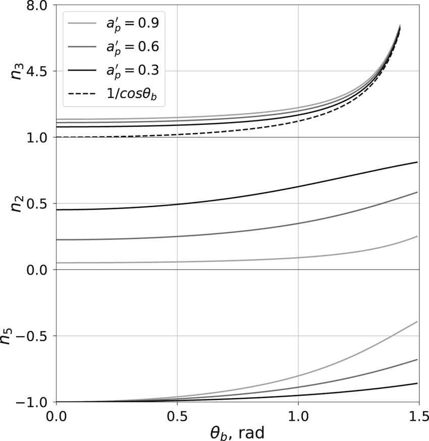
The dependencies of $n_2$, $n_3$ and $n_5$ on the angle $\theta _{b}$ are presented in figure 10. As was already shown, for $\theta _{b} = 0$ ($\cos \theta _{b} = 1$) we have $n_{2,3} = 1 \pm (a_{p}^{\prime })^{1/2}$. But for $\theta _{b} = {\rm \pi} /2$, ($\cos \theta _{b} = 0$) we obtain $n_2 = (1-a_{p}^{\prime })^{1/2}$ and $n_3 \to 1/\cos \theta$, the superluminal mode $j = 2$ transforming into a purely transverse wave. As for the wave $j = 5$, which was not mentioned earlier, it is a wave propagating in the negative direction in the laboratory reference frame, and is purely transverse: $n_{5} = -1$ at $\theta _{b} = 0$ and $n_{5} = - (1 - a_{p}^{\prime })^{1/2}$ at $\theta _{b} = {\rm \pi} /2$. This mode occurs as a result of Lorentz transformation of the frequency and wavevector of a wave propagating in a positive direction in a rest frame into a laboratory frame.

Figure 10.

Refractive indices $n$ for modes $j = 2, 3, 5$. The parameter $a_{p}^{\prime } = \langle \omega_{\rm pe}^2/(u^{3}\omega ^2)\rangle$. The dashed line corresponds to $n=1/\cos \theta _{b}$.

Returning now to the question of wave attenuation, we note that for $\varDelta \ll u_{0}$ the attenuation of the plasma-Alfvén wave $j = 3$, as for cold plasma, begins only at angles $\theta _{b} > \theta ^{\ast }$. As for the attenuation of the Alfvén mode $j = 4$ ($n\cos \theta \simeq 1$), for this mode the second term in brackets in (6.3) cannot be neglected. As a result, the integral becomes equal to

(6.15)\begin{equation} \int\left[ 1 + \frac{n\cos\theta_b}{2u^2(1-n\cos\theta_b)}\right]^{{-}1}\frac{\textrm{d}F}{\textrm{d}u} \,\textrm{d}u = \int\frac{u^2}{u^2-u_r^2-\mathrm{i}0}\frac{\textrm{d}F}{\textrm{d}u} \, \textrm{d}u. \end{equation}

Here the quantity $u_r$ is the resonant momentum

(6.16)\begin{equation} u_r^2 = \frac{n\cos\theta_{b}}{2(n\cos\theta_{b}-1)}, \end{equation}

and we added a small imaginary part in the denominator to take into account the Landau bypass rule for the pole $(\omega \to \omega + \mathrm {i} 0)$, i.e. for the refractive index $n \to n-\mathrm {i}0$. Thus, the dispersion equation takes the form

(6.17)\begin{equation} 1 - n^2 + \frac{\omega_\textrm{pe}^2}{\omega^2}\frac{1+n\cos\theta_{b}}{n\cos\theta_{b}}\left[{\int\kern-10pt} \left.\frac{u^2}{u^2-u_r^2}\frac{\textrm{d}F}{\textrm{d}u} \, \textrm{d}u +\mathrm{i}\frac{{\rm \pi} u_r}{2}\frac{\textrm{d}F}{\textrm{d}u}\right|_{u=u_r}\right] = 0. \end{equation}

Substituting now the derivative $\textrm {d}F/\textrm {d}u$ from (6.2) and, again, introducing the notation

(6.18)\begin{equation} x = n\cos\theta_{b} - 1, \end{equation}

we obtain

(6.19)\begin{equation} \tan^2\theta_{b} +\frac{2x}{\cos^2\theta_{b}} - \frac{4\omega_\textrm{pe}^2u_{0}}{\omega^2}\left[\log\left(1-\frac{1}{2xu_{0}^2}\right) - \mathrm{i}{\rm \pi}\right]x = 0. \end{equation}

It should be borne in mind that the value $x$ in the argument of the logarithm is a complex quantity. Therefore, the logarithm is complex also, and it does not contain a module in its argument.

As a result, one can see that for not very small angles $\theta _{b} > u_0^{-2} \simeq 10^{-4}$ and the condition $u_0^2 \, a_{p}^{\prime } \gg 1$ we obtain

(6.20)\begin{equation} x = \mathrm{i}\frac{\tan^2\theta_{b}}{4{\rm \pi}}\frac{\omega^2}{u_{0}\omega_\textrm{pe}^2}. \end{equation}

Thus, the imaginary part of the refractive index of the Alfvén mode is

(6.21)\begin{equation} \textrm{Im} (n_4 \cos\theta_{b}) = \frac{\tan^2\theta_{b}}{4{\rm \pi}} \frac{\omega^2}{u_0\omega_\textrm{pe}^2}\simeq \frac{\tan^2\theta_{b}}{2{\rm \pi}}A_{p}^{{-}1}, \end{equation}

which corresponds to the attenuation of the wave during its propagation in the magnetosphere.

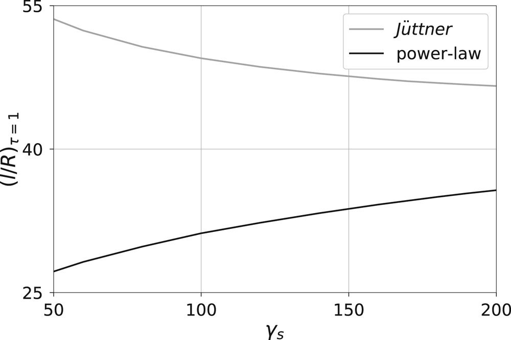
Figure 11 shows how the levels $l = r_{d}$ at which the optical depth $\tau = 1$ (4.8) depend on parameter $\gamma _{s}$ for both Jüttner ($\rho = 4$, $\gamma _{s}$) and power-law ($u_0 = \gamma _{s}/2$) distribution functions. As we see, these levels do not differ so drastically. This is due to the fact that in both cases the attenuation is determined by resonant particles whose energy is not much higher than the average particle energy.

Figure 11.

Comparison of levels $l = r_{d}$ at which the optical depth $\tau = 1$ (4.8) depending on parameter $\gamma _{s}$ for both Jüttner ($\rho = 4$, $\gamma _{s}$) and power-law ($u_0 = \gamma _{s}/2$) distribution functions for the Alfvén mode $j = 4$.

Thus, in general, the properties of four normal waves depend weakly on the particle distribution function. On the other hand, we considered it necessary to stress here that in a magnetized, relativistic streaming plasma of the radio pulsar magnetosphere in the laboratory frame, i.e. in the frame associated with a neutron star, there are six modes depending on the polarization of the wave and the direction of their propagation. For $A_{p} \gg 1$ they are two transverse electromagnetic modes with the wave electric field polarization directed orthogonal to magnetic field with the refractive index ($n_1 = \pm 1$), two electromagnetic waves with polarization directed in the plane of the magnetic field and the wavevector (Alfvén wave with refractive index $n_{4}$, and the fifth mode with $n_5 < 0$) and two plasma waves with longitudinal polarization (along the magnetic field) at $\theta _{b} = 0$ and turning into transverse wave at $\theta _{b} = 90^{\circ }$ for $n_2$ and to Alfvén wave for $n_3$.

It should be also noted that for a symmetric distribution function $F(u)$ with respect to the zero momentum, $u = 0$, $F(u) = F(-u)$, in the plasma rest frame, the dispersion equation (2.17) can be presented in the form

(6.22)\begin{equation} 1-n^2+2\frac{(1-n^2\cos^2\theta_b))\omega^2_p}{\omega^2}\int_0^\infty\frac{\beta {\textrm{d}F/\textrm{d}u}}{1-n^2\beta^2\cos^2\theta_b}\textrm{d}u=0, \end{equation}

from which one can see that it has two roots of $n^2$, which means that there are, as it were, two modes of oscillations. Adding the mode $n_1^2 = 1$, the total number of modes is three. However, this is not so because $n = \pm (n^2)^{1/2}$, and the number of modes is six. The degeneracy is removed for the streaming distribution function, $F(u) \neq F(-u)$. Thus, the consideration of eigenmodes in the laboratory coordinate frame gives the same picture as the consideration in the rest frame.