Nomenclature
-
 $\mathrm{A}_{1e}$
-
effective flow area just upstream of shock train (m2)
- d
-
ray transverse displacement (m)
-
f
$_{d}$
-
focal length of decollimating lens (m)
- h
-
duct half height (m)
-
h
$_{th}$
-
throat half height (m)
- Hue
-
hue (deg)
- K
-
Gladstone-Dale constant (m3/kg)
- L
-
spanwise width (m)
- M
-
Mach number
-
M
$_{1\infty}$
-
freestream Mach number just upstream of shock train
- n
-
power law index
- p
-
wall pressure (Pa)
-
p
$_{os}$
-
stagnation pressure in plenum chamber (Pa)
-
p
$_{1}$
-
static pressure just upstream of shock train (Pa)
-
p
$_{b}$
-
back pressure (Pa)
- Re/m
-
unit Reynolds number (m-1)
-
T
$_{b}$
-
ambient temperature (K)
-
u
$_{1}$
-
streamwise velocity inside boundary layer (m/s)
-
u
$_{1\infty}$
-
streamwise freestream just upstream of shock train (m/s)
- x
-
spanwise distance (m)
- y
-
vertical distance (m)
- z
-
streamwise distance from test section inlet (m)
-
z
$_{0}$
-
fixed streamwise location (m)
-
z
$_{1}$
-
streamwise location just upstream of shock train (m)


Greek symbol
-
$\gamma$
-
specific heat ratio
-
$\delta_{1}$
-
boundary layer thickness just upstream of shock train (m)
-
$\delta_{1}^{*}$
-
displacement thickness just upstream of shock train (m)
-
$\epsilon$
-
deflection angle of light ray (rad)
-
$\eta$
-
normal distance from duct wall (m)
-
$\theta_{1}$
-
momentum thickness just upstream of shock train (m)
-
$\rho$
-
density (kg/m3)
-
$\rho_{os}$
-
stagnation density in plenum chamber (kg/m3)
-
$\rho_{1}$
-
density inside boundary layer just upstream of shock train (kg/m3)
-
$\rho_{1\infty}$
-
freestream density just upstream of shock train (kg/m3)
-
$\rho_{b}$
-
ambient density (kg/m3)


1.0 Introduction
Over the past few decades, the development of dual-mode scramjet engines for realising next-generation propulsion systems has been consistently investigated. A dual-mode scramjet engine provides a practical solution to supersonic flight by operating over a wide range of Mach numbers. In the ramjet mode, the incoming air is compressed through a series of shock waves (i.e. precombustion shocks) in the isolater before entering the combustion chamber. This process is critical to determine overall engine performance, and thus numerous studies of the isolator shock train have been carried out in the context of design optimisation of scramjet engines [Reference Gnani, Zare-Behtash and Kontis1]. In fact, such a repeated shock structure appears in a variety of flow-devices such as supersonic wind tunnels, supersonic ejectors, and supersonic inlets of aircraft engines [Reference Matsuo, Miyazato and Kim2]. Furthermore, these repeated shock structures have been called in many different ways in the literature including terms such as “multiple shocks”, “shock system”, and a series of shocks. As used herein, we refer to the shock structures in this study as a “shock train” [Reference Matsuo, Miyazato and Kim2]. A shock train is usually followed by a mixing region, in which the static pressure recovery takes place if the duct length is sufficient. The whole interaction region including both the shock train and the mixing region is called a “pseudo-shock”. However, it is often seen that the technical terms, shock train and pseudo-shock, have been used in a confusing manner.
The previous studies [Reference Gnani, Zare-Behtash and Kontis1, Reference Matsuo, Miyazato and Kim2] show that a shock train occurs as a result of the interaction of a normal shock with a boundary layer developing along the wall surface in a confined duct. In almost all the previous experimental investigations, shock trains have been studied primarily by the wall pressure measurements coupled with the schlieren or shadowgraph visualisations. A primary characteristic of a shock train is determined by the pressure rise due to the shock train, the distance between the successive shocks in a shock train, the number of the shocks constituting a shock train, and the longitudinal length of a shock train. These factors are significantly influenced by three main parameters just upstream of the shock train. The first is the freestream Mach number (
 $M_{1\infty}$
). The second is the Reynolds number based upon the boundary layer characteristic length (e.g. the boundary layer thickness,
 $\delta_{1}$
, or the boundary layer momentum thickness,
 $\theta_{1}$
). The third is the blockage ratio or the boundary layer relative thickness or the flow confinement parameter, which can be defined as the ratio
 $\delta_{1}/h$
of the boundary layer thickness
 $\delta_{1}$
to the duct half height, h, for a two-dimensional duct or a circular duct radius [Reference Carroll and Dutton3]. In addition, it is well-known that shock waves inside a shock train oscillate across these time-mean positions and induce strong pressure fluctuations, leading to vibration of the fluid machines or significant noise emitting into the surrounding air [Reference Gnani, Zare-Behtash and Kontis1, Reference Matsuo, Miyazato and Kim2]. Recently, understanding of the behaviour of an unsteady shock train is of great need in the context of the design of scramjet engines since a higher engine thrust can be achieved when a shock train is confined inside the isolator of the scramjet engine [Reference Xiong, Fan, Wang and Tao4–Reference Hou, Chang, Xie, Wang, Wu and Bao6]. Furthermore, shock train oscillations have a significant effect on the unstart problem.
The high-speed schlieren [Reference Xiong, Fan, Wang and Tao4, Reference Hou, Chang, Xie, Wang, Wu and Bao6, Reference Gawehn, Gülhan, Al-Hasan and Schnerr7] and high-speed shadowgraphy [Reference Grzona and Olivier8] were previously used to investigate the shock train oscillations. However, the focus of those studies was on the vibration of the shock itself, and thus the unsteady flow field around shocks can not be measured at the same time. The Laser-Doppler-Velocimeter (LDV) [Reference Carroll and Dutton3, Reference Sugiyama, Arai, Abe, Takahashi and Takayama9] and the stereo particle image velocimetry [Reference Hunt and Gamba5] are also promising approaches to investigate the internal structures of a shock train. However, the laser-based velocimetry shows that the seed particles do not seem to follow the sudden change in the velocity fields just behind the shock [Reference Koike, Suzuki, Kitamura, Hirota, Takita, Masuya and Matsumoto10, Reference Wernet11]. Conventional schlieren techniques [Reference Settles12, Reference Settles and Hargather13] have been limited to use only for qualitative visualisation of the flow fields inside a shock train since it requires a cumbersome process to extract the two-dimensional density field from schlieren images. For validation purpose of the computational scheme, these experimentally measured schlieren images are often compared with the simulated ones [Reference Sun, Sugiyama, Mizobata and Fukuda14–Reference Gnani, Zare-Behtash, White and Kontis18]. Due to difficulty of obtaining the quantitative information of the flow fields inside the shock train, it is often seen that the measured wall pressure distribution is used for validation of the computational methodology [Reference Morgan, Duraisamy and Lele16, Reference Gnani, Zare-Behtash, White and Kontis18–Reference Gnani, Zare-Behtash, White and Kontis20]. It is worth mentioning that although a good agreement between the measured and simulated wall pressure distributions or schlieren images can be achieved, the computed scalar quantities or vector fields inside the shock train could be still inaccurate. Despite of significant progress made in the experimental apparatuses, the flow measuring techniques, and the computational methods, the detailed structures inside a shock train still remain elusive.
Recently, with the development of the improved digital image processing and computational capability, several schlieren-based quantitative flow visualisations have been developed such as the background oriented schlieren (BOS) [Reference Nicolas, Donjat, Léon, Le Besnerais, Champagnat and Micheli21], the rainbow schlieren deflectometry (RSD) [Reference Takano, Kamikihara, Ono, Nakao, Yamamoto and Miyazato22–Reference Mariani, Lim, Zang, Vevek, New and Cui25], and the calibrated schlieren [Reference Nazari, Ishino, Ishiko, Ito, Kondo, Yamada, Motohiro, Miyazato and Nakao26]. However, most of these techniques for obtaining the density fields of shock-dominated flows have been limited to supersonic free jets. Therefore, the goal of this paper is twofold. First, a novel technique is developed for obtaining the two-dimensional density field with the shock-wave/boundary-layer interaction (SWBLI) using the rainbow schlieren deflectometry because of simple, easy to use, and relatively inexpensive in which a rainbow filter with fine colour gradations only is utilised instead of using a knife edge in a conventional schlieren system [Reference Settles12, Reference Settles and Hargather13]. Furthermore, the rainbow schlieren makes it feasible to perform a quantitative evaluation of certain refractive index fields such as shock-dominated and turbulent flows by relatively simple calculations. Second goal is to apply the proposed technique for a shock train in a confined duct. This configuration is particularly interesting since a normal shock in any fluid device with high-pressure gases tends to interact with a boundary-layer and to form a shock train in most cases. The quantitative information of the detailed structures of the flow fields inside a shock train is valuable for validating a variety of numerical simulation codes in this community. Note that there is no access to an analytical model which can quantitatively predict the quasi-periodic wavy features from successive shocks inside a shock train. In almost all previous studies, any quantitative information about the flow fields inside the shock train were not provided, and only the flow properties just downstream of a pseudo-shock were calculated for known incoming flow parameters such as the freestream Mach number, flow confinement parameter, and Reynolds number just upstream of the shock train [Reference Matsuo, Miyazato and Kim2]. The present study focuses on the instantaneous structure of the density field including a shock train and the following mixing region (i.e. pseudo-shock).
2.0 Experimental setup
2.1 Experimental apparatus
The experiments were performed at the intermittent blowdown compressed-air facility of the High-Speed Gasdynamics Laboratory at the University of Kitakyushu. A schematic diagram of the experimental apparatus with the rainbow schlieren system is shown in Fig. 1. Ambient air is pressured by the compressor up to 1 MPa, and then stored in the high-pressure reservoir consisting of two storage tanks with a total capacity of 2m3 after being filtered and dried. The supply line from the reservoir can be connected to the plenum chamber through the coupling as shown in Fig. 1. The high-pressure dry air from the reservoir is stagnated in the plenum chamber and then discharged into the atmosphere through the Laval nozzle and the test section. The plenum pressure is controlled and maintained constant during the testing with the valve.
Schematic drawing of experimental apparatus with rainbow schlieren optical system.

Figure 2 shows a schematic of the Laval nozzle that is designed for Mach number = 1.5. The heights at the throat and exit are 4.24 and 5mm, respectively, and a constant spanwise width of L = 13mm over the full length from the nozzle inlet to exit. The shape of the Laval nozzle was generated by the method of characteristics [Reference Crown27] to provide uniform and parallel flow at the nozzle exit. The test section is directly connected to the exit of the Laval nozzle and consists of a constant-area straight duct with a height of 2h = 5mm and a width of L = 13mm. There are 40 static pressure measuring locations with a tap of 0.5mm in diameter along the centre line of the upper wall at an equal interval of 1mm over the range from z = 0mm to z = 39mm. Each static pressure tap is connected to the digital pressure sensor (Yokogawa Model MT220) with uncertainty of 50Pa through a polyvinyl chloride tube with an inner diameter of 0.7mm and a length of 500mm. The region enclosed by the red dashed line in Fig. 2 indicates the range of an optical window for flow visualisation by the rainbow schlieren deflectometry. The operating pressure ratio of plenum pressure
 $p_{os}$
to back pressure
 $p_{b}$
(= 102.8kPa
 $\pm\;0.5$
kPa) was held constant at 1.8 within an accuracy of
 $\pm\;0.1 \%$
to produce a shock train in the test section where the room temperature
 $T_{b}$
was 293.7K
 $\pm\;0.1 \textrm{K}$
.
Laval nozzle and test section. All dimensions are in mm.

2.2 Rainbow schlieren optical system
As shown in Fig. 1, the rainbow schlieren system is composed of rail-mounted optical components including the continuous 250W metal halide light source (Sigmakoki IMH-250) connected to the spatial filter with a 3mm
 $\times \;50\mu \mathrm{m}$
rectangular slit through a
 $\;50\mu \mathrm{m}$
diameter optical fiber, the collimating and decollimating lenses with 50mm diameter and 500 mm focal length, the rainbow filter, and the digital camera (Nikon D7100, effective pixels 24.1 million). Rainbow schlieren pictures were taken with an exposure time of 1/8,000s and ISO 640. Takeshita et al. [Reference Takeshita, Nakao and Miyazato28] experimentally observed that a shock train with an incoming Mach number of 1.44 oscillates around its time-mean position with a dominant frequency of around 10Hz. Therefore, the exposure time of the present rainbow schlieren system should be short enough to freeze a shock train.
Figure 3 shows a schematic drawing of the part of the present rainbow schlieren system. In the rainbow schlieren system, when a collimated light ray is deflected through the test area, a colour image of the area revealing the ray deflections is formed on the recording medium of the digital camera. The schlieren image of the test area is then digitised to acquire a direct quantification of the light deflections using the calibration curve of the rainbow filter. The image of the rainbow filter used in the present experiments is shown in Fig. 4. In the previous preliminary experiment with the rainbow filter of 1.4mm wide [Reference Takeshita, Takano, Ono, Nakao and Miyazato29, Reference Matsuyama, Nakao, Ono, Miyazato and Kashitani30], it was found that the deflection angle of light ray after passing through the region with a strong density gradient inside a shock train exceeds the upper limit of the rainbow filter. Therefore, a new rainbow filter with a 2.5mm wide strip and continuous hue variation from Hue = 0 to 350 deg was fabricated in the present study.
Rainbow schlieren optical system.

Image of rainbow filter.

Two sets of rainbow schlieren pictures were taken. In the first set, the rainbow filter was arranged in such a manner that the hue changes perpendicular to the z direction (called the vertical cutoff setting, herein). The vertical cutoff setting is design to render the streamwise density gradients. While for the second set, the rainbow filter was arranged in such a manner that the hue changes parallel to the z direction (called the horizontal cutoff setting, herein). The horizontal cutoff setting should render transverse density gradients. The characteristics of the rainbow filter were performed by automatically traversing the filter in intervals of 20
 $\mu \mathrm{m}$
 $\pm\;1\mu \mathrm{m}$
at the schlieren cutoff plane (i.e. the location of the focal point of the decollimating lens) before starting experiments.
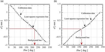
The calibration curves of the rainbow filter for the vertical cutoff setting and the horizontal cutoff setting are shown in Figs 5(a) and (b). The open symbols express the experimental data with precision error bars. The solid line indicates a least squares regression of the experimental data. The background hue in the rainbow filter for the present experiment corresponds to the location shown as the red arrow in each plot. The calibration of the rainbow filter in the present study was performed by traversing the filter at the schlieren cutoff plane. Settles and Hargather [Reference Settles and Hargather13] proposed the different type of the filter calibration by placing a calibration object with a known refractive index variation in the location of the schlieren object. Thus, it is feasible to perform a direct conversion from image pixel intensity to the corresponding refractive index gradient value. For instance, Mariani et al. [Reference Mariani, Zang, Lim, Vevek, New and Cui24, Reference Mariani, Lim, Zang, Vevek, New and Cui25] implemented a filter calibration using a single weak focal-length lens as the calibration object. The more detailed explanation about how to design, generate, and calibrate a rainbow filter can be found elsewhere [Reference Agrawal and Wanstall31].
Calibration curves of rainbow filters of (a) vertical and (b) horizontal cutoff settings.

3.0 Reconstruction of density fields
Light rays coming from the decollimating lens after travelling the test section without air flows passes through a fixed location of the background hue on the rainbow filter. As shown in Fig. 3, if air flows with density gradients (e.g. shock trains) are present in the test section, some parts of the light rays are deflected from the original optical paths while traveling the test section. Carroll and Dutton [Reference Carroll and Dutton3] investigated the effects of the flow confinement parametre
 $\delta_{1}/h$
on the characteristic of a shock train by varying
 $\delta_{1}/h$
= 0.08 to 0.49 at two freestream Mach number conditions (
 $M_{1\infty}$
= 1.6 and 2.45). Under the condition of
 $M_{1\infty}$
= 1.6 and
 $\delta_{1}/h$
= 0.40, the surface oil flow visualisations on the duct upper as well as lower walls indicates two-dimensional flow structures in the whole flow field of the shock train except for the small corner regions beneath the foot of the first shock. Atkin and Squire [Reference Atkin and Squire32] have studied the shock-wave/boundary-layer interaction over a range of freestream
 $M_{1\infty}$
= 1.3 to 1.5 and found that static pressure distributions measured along the tunnel span downstream of a shock shows essentially two-dimensional flows over the middle 88 % of the tunnel width. Additionally, the flow structures in the downstream of a shock with
 $M_{1\infty}$
= 1.5 maintains the two dimensionality across the tunnel span except for a small region near the side walls. From these observations, it is assumed that the flow properties in the spanwise direction (x direction) remain constant so that the effects of the side wall boundary layers are negligible.
The deflection angle
 $\varepsilon$
of a light ray just after passing through the test section is given by the following relation based on the geometrical optics as:
 \begin{equation} \varepsilon(z, y)=\frac{d(z, y)}{f_{d}}, \end{equation}
where y is the vertical distance from the duct centreline, z is the streamwise distance from the test section inlet,
 $f_d$
is the focal length of the decollimating lens and d(z, y) is the ray transverse displacement from the location of the background hue. Here, the direction of the displacement is identical to that of the hue variation on the rainbow filter.
For a rainbow schlieren picture obtained by the vertical cutoff setting, the density gradient in the flow direction (z axis) at the duct centreline (y = 0) after passing through the test section with a width of L (= 13mm) is given by:
 \begin{equation} \frac{\partial \rho(z, 0)}{\partial z}=\frac{\varepsilon(z, 0)}{K L}, \end{equation}
where
 $K\left(=2.26 \times 10^{-4} \mathrm{\;m}^{3}/ \mathrm{\;kg}\right)$
is the Gladstone-Dale constant. Note that the Gladstone-Dale constant has a weak dependence on the wavelength of light [Reference Agrawal and Wanstall31], the same value can be used. Similarly, for a rainbow schlieren picture obtained by the horizontal cutoff setting, the density gradient in the vertical direction (y axis) for a fixed
 $z = z_0$
is given by
 \begin{equation} \frac{\partial \rho\left(z_{0}, y\right)}{\partial y}=\frac{\varepsilon\left(z_{0}, y\right)}{K L}, \end{equation}
Integration of (2) with respect to z yields the density distribution in the z direction along the duct centreline:
 \begin{equation} \rho(z, 0)=\frac{1}{K L} \int_{0}^{z} \varepsilon(z, 0) d z+\rho(z_1,0), \end{equation}
where
 $\rho(z_1,0)$
corresponds to the density just upstream (
 $z = z_1$
) of the shock train, and it can be estimated from the isentropic relation between the plenum pressure and the wall pressure at the location where the shock train is produced.
Integration of (3) with respect to y leads to
 \begin{equation} \rho\left(z_{0}, y\right)=\frac{1}{K L} \int_{0}^{y} \varepsilon\left(z_{0}, y\right) d y+\rho\left(z_{0}, 0\right). \end{equation}
Given
 $z = z_0$
, combining (4) and (5) reconstructs the one-dimensional density profile,
 $\rho(z_0,y)$
. This process is repeated by changing the streamwise locations (
 $z_0$
) in order to calculate the two-dimensional density field (i.e.
 $\rho(z,y)$
) of the whole interaction region including the shock train.
4.0 Flow properties just upstream of shock train
Previous studies [Reference Matsuo, Miyazato and Kim2, Reference Om and Childs33–Reference Yamane, Oshima, Nakamura, Ishii and Park35] show that the structures of a shock train are significantly affected by the undisturbed flow properties such as the freestream Mach number (
 $M_{1 \infty}$
), boundary layer properties, Reynolds number, etc. However, there is not much information available in the literature as to how to experimentally obtain these primary parameters. A brief explanation how to calculate these quantities is provided below. First, the adiabatic flow is assumed through all the flow fields including a shock train. This implies that the total temperature should remain constant throughout the whole flow field. The freestream Mach number(
 $M_{1 \infty}$
) just upstream of the shock train can be determined based on the isentropic flow assumption at the outer edge of boundary layers from the plenum chamber to the location just upstream of the shock train. Assuming that there is zero pressure gradient across the boundary layers and using the measured wall pressure
 $p_{1}/p_{os}$
normalised by the plenum pressure
 $p_{os}$
, one can calculate
 $M_{1 \infty}$
as follows:
 \begin{equation}M_{1 \infty}=\sqrt{\frac{2}{\gamma-1}\left[\left(\frac{p_{o s}}{p_{1}}\right)^{\frac{\gamma-1}{\gamma}}-1\right].}\end{equation}
In order to simplify the problem, it is assumed that the effect of the boundary layer at the nozzle throat is negligible, and that the displacement thickness (
 $\delta_1^{*}$
) of the boundary layer just upstream of the shock train is the same at the upper, lower, and side walls. If
 $A_{1e}$
is the effective flow area just upstream of the shock train and
 $2h_{th}L$
(
 $h_{th}$
is the half height of the throat) is the cross-sectional area of the throat, the continuity equation between the locations of the throat and just upstream of the shock train leads to
 \begin{equation}A_{1 e}=\frac{2 h_{t h} L}{M_{1 \infty}}\left[\frac{(\gamma-1) M_{1 \infty}^{2}+2}{\gamma+1}\right]^{\frac{\gamma+1}{2(\gamma-1)}}.\end{equation}
The difference between the duct geometrical area (2hL) and the effective flow area (
 $A_{1e}$
) is given by
 \begin{equation}2 h L-A_{1 e}=\left(L-2 \delta_{1}^{*}\right)\left(2 h-2 \delta_{1}^{*}\right).\end{equation}
Substitution of (7) into (8) leads to
 \begin{equation}\frac{\delta_{1}^{*}}{h}=\frac{1+\displaystyle\frac{L}{2 h}-\displaystyle\sqrt{\left(1+\frac{L}{2 h}\right)^{2}-\frac{2 L h_{t h}}{M_{1 \infty} h^{2}}\left[\frac{(\gamma-1) M_{1 \infty}^{2}+2}{\gamma+1}\right]^{\frac{\gamma+1}{2(\gamma-1)}}}}{2}.\end{equation}
For a boundary layer of compressible flow over a flat-plate, the ratio between the displacement thickness and the boundary layer thickness
 $\delta_{1}^{*}/\delta_{1}$
is defined by:
 \begin{equation} \frac{\delta_{1}^{*}}{\delta_{1}} \equiv \int_{0}^{1}\left(1-\frac{\rho_{1} u_{1}}{\rho_{1 \infty} u_{1 \infty}}\right) d \left(\frac{\eta}{\delta_{1}}\right), \end{equation}
where
 $\eta$
denotes the normal distance from the duct wall,
 $\rho_{1 \infty}$
is the freestream density, and
 $u_{1} = u_{1}(\eta)$
and
 $u_{1 \infty}$
are the streamwise velocities inside the boundary layer and at the outer edge of the boundary layer, respectively.
The density inside the boundary layer normalised by the freestream density can be derived based on the assumptions of the constant total temperature and static pressure across the boundary layer with the equation of state for the perfect gas as follows [Reference Tuchker36]:
 \begin{equation} \frac{\rho_{1}}{\rho_{1 \infty}}=\frac{1}{1+\displaystyle\frac{\gamma-1}{2} M_{1 \infty}^{2}\left[1-\left(\frac{u_{1}}{u_{1 \infty}}\right)^{2}\right]}. \end{equation}
The one-nth power velocity profile is assumed inside the boundary layer by
 \begin{equation} \frac{u_{1}}{u_{1 \infty}}=\left(\frac{\eta}{\delta_{1}}\right)^{1 / n}, \end{equation}
with
 $u_{1} = u_{1 \infty}$
for
 $\delta_{1} \leq \eta \leq h$
Although the power law index, n, generally depends on the Reynolds number [Reference Gerhart, Gross and Hochstein37], a value of n = 7 is specified in the present study. In the case of n = 7, substitution of (11) and (12) into (10) leads to
 \begin{equation}\frac{\delta_{1}^{*}}{\delta_{1}}=1-7(D-1)\left[\frac{D^{3}}{2} \ln \left(\frac{D}{D-1}\right)-\frac{D^{2}}{2}-\frac{D}{4}-\frac{1}{6}\right],\end{equation}
with
 $\displaystyle D \equiv 1+\frac{2}{(\gamma-1) M_{1 \infty}^{2}}$
[Reference Matsuyama, Nakao, Ono, Miyazato and Kashitani30]. Note that (10) and (11) can be also used for laminar boundary layer if the velocity profiles of the laminar boundary layers are assumed in (12).
5.0 Results and discussion
5.1 Flow visualisation
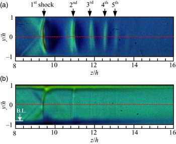
A typical rainbow schlieren picture of a shock train is presented in Fig. 6 for the case with the plenum pressure
 $p_{os}$
is 185.0kPa, the back pressure
 $p_{b}$
=102.8kPa, and the atmospheric temperature
 $T_{b}$
is 293.7K. The flow direction is from left to right. The abscissa and ordinate denote the normalised streamwise distance from the test section inlet (the exit of the Laval nozzle) and the normalised vertical distance from the duct centreline, respectively. The red dashed line in Fig. 6 shows the duct centreline (
 $y/h$
= 0). The freestream Mach number
 $M_{1 \infty}$
is 1.42, the flow confinement parameter (the boundary layer relative thickness)
 $\delta_{1}/h$
is 0.175, the unit Reynolds number
 $Re/m$
is
 $2.99 \times 10^{7}\mathrm{\;m}^{-1}$
just upstream of the shock train. These quantities characterising a shock train were calculated using the method described in Section 4 with the measured wall pressure in Subsection 5.2.
Schlieren pictures with rainbow filter of (a) vertical and (b) horizontal cutoff settings. Boundary layer thickness shown in (b) is estimated from transverse density profile.

Figure 6(a) was taken with a rainbow filter of the vertical cutoff setting to visualise the density variation in the flow direction (z direction). The overall structures of the shock train are clearly captured in this picture. The shock train consists of about five shocks as indicated in Fig. 6(a) by the down-pointing arrows. The shock train is nearly symmetrical with respect to the duct centreline. The first shock is bifurcated into a leading oblique shock and a rear oblique shock. As a result, there is a small normal part of the shock front near the duct centreline. The shocks following the first shock (i.e. the secondary shocks) are almost normal to the duct centreline. Figure 6(b) was taken with a rainbow filter with the horizontal cutoff setting to visualise the density variation in the vertical direction (y direction). The streamwise variation of the outer edge of the boundary layer can be clearly observed in this picture. The boundary layer thickness rapidly increases across the first shock and then decreases until it starts increasing again due to the effect of the second shock. This process repeats over the successive shocks. Consequently, there are unique feature of bumps of the boundary layer outer edge formed at each shock in the shock train.
5.2 Wall pressure distribution
The streamwise wall pressure distribution along the centreline of the duct top wall is shown with the open symbols in Fig. 7. At each measuring location, 100 data points were collected for 0.1s at the sampling rate of 1kHz and then time averaged. Similar measurements were repeated five times in order to obtain the ensemble average.
Streamwise wall pressure distribution.

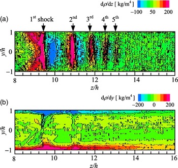
Two-dimensional shock train structure represented with (a) steamwise density gradient and (b) transverse density gradient.

In the plots, the symbol size represents the estimated experimental uncertainty. The abscissa is the normalised streamwise distance,
 $z/h$
, from the duct inlet (i.e. the exit of the Laval nozzle), and the ordinate is the ratio of the wall static pressure p to the plenum pressure
 $p_{os}$
. The theoretical static pressure jump, which is calculated using the Rankin-Hugoniot relation for
 $M_{1 \infty}$
= 1.42, is shown as a reference (the blue vertical arrow). The arrow on the right vertical axis shows a value of the back pressure normalised by the plenum pressure (
 $p_{b}/p_{os}$
= 0.556). In the wall pressure profile, the arrows indicate the locations of each shock in the shock train. Note that these locations were obtained from the streamwise distribution of the density gradient on the centreline of the duct as shown in Fig. 9. It is observed that these locations are consistent with the ones from the schlieren image of Fig. 6(a).
In the upstream region between the duct inlet and the first shock of the shock train, the wall pressure gradually increases due to the effect of the wall friction under the supersonic flows through a constant-area channel [Reference Shapiro38]. The wavy distribution is due to the Mach waves originated from the nozzle exit. There is a sudden increase in the wall pressure by the presence of the first shock. Note that there is no kink point at the position of the first shock as characterised by the shock-induced boundary layer separation [Reference Seddon39]. It means that no boundary layer separation occurs at the foot of the first shock. In the wall static pressure distribution after the first shock, no distinctive changes can be observed. The theoretical pressure ratio based on the Rankine-Hugoniot relation is 0.67 for
 $M_{1 \infty}$
= 1.42 while the measured value at the location of the fifth shock of the shock train is about 0.52. The wall pressure keep raising toward the duct exit until it reaches the back pressure. The pressure recovery caused by the shock train is about 78% of the theoretical value of a single normal shock for the same incoming Mach number. The lower pressure recovery obtained in the experiment might be attributed to the effective area reduction due to the boundary layer growth starting at the start of the interaction [Reference Matsuo, Miyazato and Kim40].
5.3 Density gradient fields
The schlieren pictures of a shock train taken using the vertical and horizontal cutoff settings of the rainbow filter can be utilised in order to obtain the streamwise and transverse density gradient fields. Figure 8(a) shows the streamwise density gradient field inside the shock train. With this cutoff setting, the distinct features of the five shocks are captured in detail. It is important that this method is able to clearly clarify the range and shape of compression and expansion regions across each shock in the shock train in the two-dimensional manner. As shown in Fig. 8(b), the flow features within the boundary layer associated with the interaction between shock-waves and the boundary-layer can be recognised by a large variation of the transverse density gradient field. The boundary layer exhibits a sharp rise followed by a sudden decrease beneath each shock of the shock train.
The streamwise distribution of the density gradient of the shock train along the duct centreline is illustrated in Fig. 9. A red open symbol indicates the exact location of each shock inside the shock train where the density gradient reaches the local maximum value. As seen in Fig. 9, the density gradient becomes negative in the expansion region between shocks, and the local minima in the density gradient distribution are shown as the blue open symbols. The streamwise density gradient distribution has a positive maximum value at the location of the first shock (at
 $z/h\sim$
9.2) and a negative minimum value behind the shock (at
 $z/h\sim$
10). The positive and negative peak values significantly decrease in the downstream region where the strength of shock and expansion waves become weaker toward the downstream direction. The shock train is defined as a series of genuine shocks followed by the mixing region when the duct is long enough [Reference Matsuo, Miyazato and Kim2]. It is important to know the exact end location of a shock train not only for the engineering and academic perspectives, but also for a better understanding of the feature of the shock train since a majority of the static pressure rise over the pseudo-shock region occurs in the shock train region [Reference Matsuo, Miyazato and Kim2, Reference Sullins and McLafferty41]. Although a shock train can be easily captured by optical observations such as schlieren or shadowgraph pictures, it is still difficult to quantitatively determine the end of the shock train using such conventional pictures. This is due to the fact that the region where shocks are visibly present is influenced by the contrast of the pictures, which depends strongly on the setting of a knife-edge in the schlieren system and so on.
Streamwise denstiy gradient profile along duct centreline.

Recently, Hunt and Gamba [Reference Hunt and Gamba5] have devised a method to find the end of a shock train from the measured wall pressure profiles. However, considering that shocks are present in the core flow away from the wall surface, it could therefore be possible that the wall pressures tend to be smeared out due to the dissipative nature of the boundary layer [Reference Gnani, Zare-Behtash and Kontis1, Reference Weiss, Grzona and Olivier42]. The current methodology avoids this issues since it can directly resolve the two-dimensional feature of the shock train, and as a result, the end of the shock train can be determined with a higher accuracy (for instance, the end of the shock train is estimated
 $z/h$
= 13.2 from Fig. 9).
5.4 Flow topology of shock train
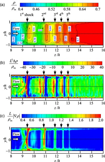
The two-dimensional density field of the shock train can be acquired by the numerical integration of the streamwise and transverse density gradient fields of the shock train. The resulting contour plot of the density field of the shock train is depicted in Fig. 10(a). The colour map over a range from
 $\rho/ \rho_{os}$
= 0.4 to 0.7 at intervals of 0.02 is provided at the top of the figure. Here,
 $\rho_{os}$
is the stagnation density in the plenum chamber. The spatial resolution of the contour is around 13
 $\mu \mathrm{m}$
. The downward arrows show the streamwise positions of shocks inside the shock train along the duct centreline, where a step density gradient is observed. This contour plot gives good qualitative and quantitative illustrations for the various critical features of the shock train. For instance, it is observed that the density contour is nearly symmetric about the duct centreline. There are several distinct regions such as upstream of the shock train, between successive downstream shocks, the mixing region downstream of the shock train, and the interaction zone near the wall surface. The density contour just upstream of the shock train is uniform outside the boundary layer with a thickness of
 $\delta_{1}/h$
= 0.175. The density profiles begin to be affected just upstream of the leading shock of the first shock. The interval between contours gradually decreases as the shock strength get weakens toward the end of the shock train. The narrowest interval (i.e. the steepest density gradient) is seen at the position of the first shock. This is consistent with the observation of Fig. 9.
Various quantitative flow visualisation for density field of shock train (a) density contour plot (b) shadowgraphy (c) bright-field schlieren.

Other quantitative visual representations can be easily extracted from the density field of Fig. 10(a). For instance, Fig. 10(b) is the shadowgraphy capturing the second spatial derivative of density, which is proportional to the Laplacian of the density. This type of technique is suitable for investigating the flow fields with strong density gradients, but not the ones with mild gradients [Reference Settles12]. Thus, shock waves can be captured well, but not expansion waves. Another drawback of using the conventional shadowgraphy is that it provides only qualitative features unlike one as shown in Fig. 10(a). In Fig. 10(b), each shock of the shock train appears as a red line followed by a blue line. The streamwise spatial evolution of the boundary layer thickness can be clearly seen as the red regions in the vicinity of the wall. Note that the image of a shock wave taken by the conventional shadowgraph system always appears as a dark line followed by a light line [Reference Liepmann and Roshko43], which shows only the general shape of the density profile through a shock wave. The bright field schlieren shown in Fig. 10(c) or the circular cut-off schlieren [Reference Settles and Hargather13] exhibits the magnitude of the density gradient vector, and it indicates the degree of compression and expansion in every directions. The bright-field schlieren highlights the shape and strength of the shock wave as well as the streamwise variation of the boundary layer thickness. It also quantitatively displays the degree of the strength of the expansion waves between the first and second shocks or between the second and third shocks.
The streamwise density distributions in the shock train are indicated in Fig. 11. The red line is the density profile along the duct centreline, while the blue line is the density profile inside the boundary layer (
 $y/h = - 0.96$
). In addition, the statistical error for the centreline density profile is depicted as the green solid line, where the error was obtained from ten experiments under the same pressure ratio (
 $p_{os}/p_{b} = 1.8$
) and normalised by
 $\rho_{os}$
. The error contains the precision error [Reference Coleman and Steele44] only, but not the bias error since it is negligibly small when compared to the precision errors. The precision error is also affected significantly by density fluctuations caused by the unsteady behaviour of the shock train [Reference Takeshita, Nakao and Miyazato28]. The red line shows that a successive sudden increase in the density is due to the presence of the successive shocks constituting the shock train. Although the density profiles gradually increase at both vertical locations, the variation of density fluctuations due to the presence of shocks is much larger along the centreline than the one inside the boundary layer. It should be noted that the density profile at the
 $y/h = -0.96$
captures the leading and rear shocks constituting the first-shock, which appears as the two broadband peaks near the first-shock. The gradual density variations are due to the weak oblique shocks. Therefore, the leading shock is not strong enough to separate the boundary layer, and the wall pressure distribution of Fig. 7 does not show a kink point near the first shock.
Streamwise density profiles at duct centrelne and inside boundary layer.

The precision error gradually increases till the location just upstream of the first shock and then abruptly increases and decreases across the first shock. The streamwise locations of the local maxima in the error profile coincide with the location of each shock in the shock train and of the maximum negative pressure gradient inside the expansion region between the successive shocks, respectively. In the downstream region of the shock train (after the fifth shock of the shock train), the error remains almost constant. Matuo et al. [Reference Matsuo, Mochizuki, Miyazato and Gohya45] experimentally investigated the oscillatory characteristics in the central region of a shock train by a static-pressure measuring system (it is called the through-tube). It was found that the distribution of the root-mean square (standard deviation) of the static pressure oscillations along the duct axis changes in a wavy form and that the peak locations agree with the time-mean positions of each shock forming the shock train. Furthermore, the maximum peak occurs at the position of the first-shock, and the following peaks gradually decrease toward the following shocks. A similar trend can be seen in the profile of the precision error shown in Fig. 11 except for the other peaks caused by the expansion waves between the successive shocks. It is challenging to capture the oscillation of the expansion waves between the successive shock by the through-tube system, since the flow fields are subject to the effect of the interaction of the shock with the unstable boundary-layer developing along the outer surface of the through-tube [Reference Grzona and Olivier8].
Transverse density profiles at three different axial locations, just ahead (
 $z/h$
= 8) and behind (
 $z/h$
= 9.6) the first shock and at the end (
 $z/h$
= 13.2) of the shock train, are shown in Fig. 12. The boundary layer relative thickness on the profile of
 $z/h$
= 8 can be determined based on the transverse density profile. The black horizontal short bar indicates the boundary layer relative thickness predicted by the method described in Section 4. The predicted value designates a location of 99 % of the freestream density. Despite the simple analytical method, it can accurately capture the boundary layer thickness. At
 $z/h$
= 9.6 (behind the first shock), the profile shows the much thicker boundary layer, which is consistent with the observation of the schlieren pictures with rainbow filter (see Fig. 6(b)). Note that this rapid increases in the boundary layer thickness might not be due to the separation bubble underneath the first shock. In the previous study by Om and Childs [Reference Om and Childs33], it was shown that both the skin-friction measurement and the alcohol technique indicate no boundary-layer separation for a shock train for the condition,
 $M_{1 \infty}$
=1.49 and
 $\delta_{1}/h$
= 0.198. In addition, Yamane et al. [Reference Yamane, Oshima, Nakamura, Ishii and Park35] performed the numeral simulation of a shock train in the similar condition (
 $M_{1 \infty}$
=1.7 and
 $\delta_{1}/h$
= 0.4) and observed only a small separation bubble near the first shock. When
 $M_{1 \infty}$
is lower than around 1.8 (the upper limit of Mach number for
 $\lambda $
- type shock train), the effect of the increased Mach number on the boundary layer is to reduce the size of the separation region, or to delay the separation [Reference Carroll and Dutton3, Reference Morgan, Duraisamy and Lele16, Reference Om and Childs33, Reference Yamane, Oshima, Nakamura, Ishii and Park35, Reference Carroll, Lopez-Fernandez and Dutton46]. Although it is hard to determine from the density profile whether or not there is a separation bubble, the separation should not happen under the present experimental condition. The transverse Mach number profiles at the two axial locations (at the start and end of the shock train), which are estimated by the density profile (Fig. 12) and the wall pressure profile (Fig. 7), are shown in Fig. 13. Note that the static pressures just ahead and behind the shock train is assumed to be constant across the duct cross-section [Reference Matsuo, Miyazato and Kim2]. It can be observed from Fig. 13 that the boundary layer relative thickness is around 0.4 at the end of the shock train, and that the Mach numbers are still supersonic. In addition, the freestream Mach number just upstream of the shock train is 1.42, agreeing with the value predicted from the wall static pressure within an accuracy of around 1%.
Transverse density profiles at selected locations inside shock train.

Transverse Mach number profiles at start and end of shock train.

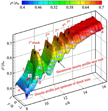
For a better understanding of the flow topology of the intricate structure of the density field inside the shock train, the bird’s eye view representation of the density field is shown in Fig. 14. It can be clearly seen that weak shocks or compression waves are formed at a zone between Points a and b just upstream of the first shock. Also, it is observed that the shock surface spanning from Points c to d is a concave, which is responsible for the incoming weak shocks. From this figure, one can also quantitatively see both the lateral density variation (e.g. the red dashed line between Points e and f) from the wall surface to the freestream region, and streamwise evolution (e.g. the blue dashed line between Points g and h) of the density inside the boundary layer beneath a shock train. To the best of our knowledge, there is not much this kind of the detailed and multi-dimensional quantitative measurement data in the literature. The newly developed rainbow schlieren deflectometry system is proved to be a very effective tool capable of obtaining the fine structure of the shock train and of providing a useful validation data for numerical studies in this community.
Bird’s eye view of density field of shock train.

The advantageous feature of the current rainbow schlieren technique is to perform density measurements in a microscale flows by changing the parts of the optical system such as a small source aperture, a decollimating lens with longer focal lengths, and a rainbow filter with finer colour gradations. More detailed descriptions of the rainbow schlieren technique and its applications can be found in Agrawal and Wanstall [Reference Agrawal and Wanstall31].
6.0 Concluding remarks
A new full two-dimensional field of view measurement technique using the rainbow schlieren deflectometry, which can quantitatively capture the density field of shock-wave/boundary-layer interaction in a confined duct, was proposed and applied for the first time to a shock train in a constant-area straight duct. The operating conditions are as follows: the freestream Mach number
 $M_{1\infty}$
was 1.42, the unit Reynolds number
 $Re/m$
was
 $2.99 \times 10^{7} \mathrm{\;m}^{-1}$
and the boundary layer relative thickness (i.e. the flow confinement parameter)
 $\delta_{1}/h$
was 0.175. The novel feature of the proposed method is to introduce the vertical and horizontal cutoff settings for the rainbow filters and to utilise the corresponding filter calibration curves simultaneously, which enable us to capture the complex features of the density gradient inside a shock train in detail.
The density field of the shock train was measured with a spatial resolution of around 13
 $\mu \mathrm{m}$
. Using only wall pressure distributions, it is unfeasible to estimate the exact locations of the shocks in a shock train only. However, the shock locations, where the density gradients reach local maxima, could be precisely determined from the measured streamwise density gradient inside the shock train. It was also able to ascertain the exact end location of a shock train. With the help of the high spatial resolution, the detailed flow topology of the density field inside the shock train including the shock-boundary layer interaction was able to be quantitatively revealed. The density field acquired from the present analysis makes it possible to create other quantitative visual representations including the shadowgraphy and the bright-field schlieren, which quantitatively clarify the shape and strength of each shock constituting the shock train, the degree of the strength of the expansion waves between consecutive shocks, and the streamwise evolution of the boundary layer thickness.
This type of detailed and quantitative measurements are desirable for the validation of numerical simulation codes and to propose a new analytical flow model that can theoretically predict the quasi-periodic wavy structure inside a shock train. The proposed technique can be easily extended for unsteady density measurements. An extension of the rainbow schlieren deflectometry for the time-dependent density field with an oscillating shock train will be a part of our future work.
Acknowledgements
The authors would like to gratefully acknowledge the assistance of graduate students Hirofumi TAKANO, Atsushi MATSUYAMA, and Takato INADOMI of the University of Kitakyushu for their invaluable support to the experimental work and exceptional skills in the fabrication of the facility.