1 Introduction
Cross-Lingual Word Sense Disambiguation aims to determine the most suitable translation for a given word from a source language to a target one. This is a particular case of the word sense disambiguation (WSD) problem that has received so much attention in the Natural Language Processing (NLP) community (Ide and Veronis Reference Ide and Veronis1998). CLWSD tries to deal with some of the difficulties of WSD, such as the scarcity of sense inventories and sense tagged corpora, by taking advantage of the shared meaning between parallel texts. Parallel corpora are considered the source of knowledge to perform the disambiguation in this work. These corpora are good resources not only for performing CLWSD, but for NLP in general (Resnik Reference Resnik2004), since parallel translations share hidden meaning that can be useful for extracting knowledge about a language, from another language richer in resources.
WSD has been frequently treated as a supervised learning problem (Màrquez et al. Reference Màrquez, Exsudero and Rigau2006; Mihalcea Reference Mihalcea2006), based on techniques that depend on scarce and expensive resources such as semantically tagged corpora or lexical databases like WordNet (Fellbaum Reference Fellbaum1998). Unsupervised techniques, in contrast, do not require those kinds of resources, and are commonly known as Word Sense Induction (WSI) techniques. Their objective is to induce the different senses of a specific word in a given text by selecting groups of words related to a particular sense of the word. This relation is usually based on the co-occurrence of those words with the target word, in the different contexts in which the target word can be found in the text.
This work uses co-occurrence graphs for solving CLWSD tasks. We will present a new unsupervised technique for building the graphs and we will test its robustness by applying it to many different languages. This new system, called CO-Graph, applies a new graph-based technique (Martinez-Romo et al. Reference Martinez-Romo, Araujo, Holthoefer, Arenas, Capitán and Cuesta2011), which selects as graph nodes the words in the corpus that ‘significantly’ co-occur in the same documents. In this way, our co-occurrence window is the whole document, what helps to improve the coverage of the system, while the precision is maintained by excluding those words whose co-occurrence rate is below the threshold defined by a null model of distribution of words among the set of documents. This graph-based technique relies on the hypothesis that a text document presents a coherent content, and hence, as a basic assumption, most of the words that can be found in the document tend to share related senses. Logically, this is not always true for all the words, so the objective is to link only those pairs of words sharing a common meaning. This is achieved by considering that two words are actually related if they frequently co-occur in the same documents. By applying these assumptions, we obtain a co-occurrence graph.
The disambiguation requires another resource that proposes a set of possible translations for the system to choose the most suitable ones. This resource will be a bilingual dictionary between those languages that take part in the disambiguation. This dictionary will also be built in an automatic, unsupervised way. Also, there exist many algorithms and techniques that can be used for combining the information offered by a bilingual dictionary and a co-occurrence graph. Some of those algorithms will be analysed, and the final results of the system will be compared to baselines and other unsupervised systems that deal with the same problem, for proving the effectiveness and robustness of our system.
The rest of the paper is organised as follows: Section 2 describes different approaches to WSD and more concretely to CLWSD, and defines the problem to be solved. Sections 3–6 describe the proposed system, detailing the different steps involved in the disambiguation process. Section 7 shows the evaluation frame and criteria, and illustrates the different experimental results obtained by the system and their comparison to other systems. Finally, conclusions and future lines of work are gathered in Section 8.
2 Background
2.1 Previous work
Parallel corpora have been previously used as a source of information to perform WSD. One of the first analyses of their potentiality for disambiguation was presented in Resnik and Yarowsky (Reference Resnik and Yarowsky1999), in which an evaluation frame and an approach for measuring the distance between senses were proposed. Diab and Resnik (Reference Diab and Resnik2002) proposed a method for automatically tagging senses in big parallel corpora, based on the use of sense inventories for each of the languages in the corpus. A supervised model that uses multilingual features for training a classifier was presented in Banea and Mihalcea (Reference Banea and Mihalcea2011). These features are extracted by translating the context of the ambiguous words to different languages. In Kazakov and Shahid (Reference Kazakov and Shahid2010), multilingual parallel corpora were used for building WordNet-like synsets from English to other languages, in order to obtain a specific type of alignment that results in a multilingual database. Synsets are merged depending on whether their edit distance is sufficiently small. The resource generated in this work is then used in Kazakov and Shahid (Reference Kazakov and Shahid2013) for performing word and phrase sense disambiguation and analysing the reduction of lexical ambiguity of English words. The works presented in Apidianaki (Reference Apidianaki2008, Reference Apidianaki2009) also make use of parallel corpora for inducing senses in an unsupervised way and creating semantic clusters for performing CLWSD. In general, it is important to consider that the diversity and number of different languages present in parallel corpora will determine the accuracy of WSD and CLWSD (Ion and Tufis Reference Ion and Tufis2004).
Some other works make use of other multilingual resources for performing WSD and CLWSD: Fernandez-Ordonez, Mihalcea and Hassan (Reference Fernandez-Ordonez, Mihalcea and Hassan2012) proposed an unsupervised approach that uses a dictionary with definitions of the different senses of ambiguous words as the only available information. This technique applies a variant of Lesk’s algorithm for identifying the combination of senses that maximise the overlapping between their definitions, given a sequence of words. Wikipedia is also a widely used resource for this kind of tasks. A word-sense disambiguated corpus was created in Reese et al. (Reference Reese, Boleda, Cuadros, Padr, Rigau, Calzolari, Choukri, Maegaard, Mariani, Odijk, Piperidis and Tapias2010) from the resources available in Wikipedia, for three different languages (Catalan, Spanish and English). In Dandala, Mihalcea and Bunescu (Reference Dandala, Mihalcea and Bunescu2013), two different approaches for extracting multilingual features were described, one of them using a machine translation system, and the other obtaining those features from the interlingual links of Wikipedia. Those multilingual approaches obtain a substantial error reduction with respect to a monolingual approach.
As we stated above, disambiguation is a crucial step for many NLP processes, machine translation (MT) being one of them. Many works in this field make use of WSD and CLWSD in their systems. In Vickrey et al. (Reference Vickrey, Biewald, Teyssier and Koller2005), some algorithms were presented for creating an initial system that solves the word translation problem (finding correct translations for words or phrases in a target language), and then this system was used to improve performance in machine translation tasks. The system is also based on parallel corpora. The integration of a WSD system inside a machine translation system was also performed in Chan, Ng and Chiang (Reference Chan, Ng and Chiang2007), improving the overall performance of the MT system on a specific task (NIST machine translation evaluation test set of 2002 and 2003).
In general, many techniques have been addressed for solving WSD and CLWSD, graph-based systems being one of the most successful approaches, as we can observe in the systems that participated in the 2010 and 2013 SemEval competitions. Some of these algorithms, such as PageRank (Brin and Page Reference Brin and Page1998), have been widely used in the literature (Agirre and Soroa Reference Agirre and Soroa2009; Mihalcea Reference Mihalcea2005; Navigli and Lapata Reference Navigli and Lapata2010). Regarding CLWSD, some recent proposals are represented by the systems participating in task 3 of the SemEval 2010 competition (Lefever and Hoste Reference Lefever and Hoste2010a) and task 10 of the SemEval 2013 competition (Lefever and Hoste Reference Lefever and Hoste2013). In these tasks, the Europarl parallel corpus (Koehn Reference Koehn2005) was proposed as the main knowledge source. In the 2010 task, two systems used supervised approaches: UvT-WSD (van Gompel Reference Van Gompel2010), applying the K-NN algorithm, and FCC (Vilariño et al. Reference Vilariño, Balderas, Pinto, Rodríguez and León2010), using a naive Bayes classifier. Those supervised proposals obtained the best results for the task. However, the results of our system will be compared to those obtained by the unsupervised systems participating in the tasks: in 2010, T3-COLEUR (Guo and Diab Reference Guo and Diab2010), based on probability tables extracted from the Europarl corpus, was the system that obtained the best results among the unsupervised approaches that took part in the competition. UHD (Silberer and Ponzetto Reference Silberer and Ponzetto2010) also builds a co-occurrence graph based on the aligned contexts of the target word. However, the main differences with our work rely on the fact that in the UHD system, graphs from different languages are merged by specific links, and the minimum spanning tree is extracted from the final graph to perform the disambiguation. The ParaSense system (Lefever, Hoste and De Cock Reference Lefever, Hoste and Cock2011) is a supervised, memory-based algorithm that builds different classifiers using both local context features and binary bag-of-words features. It was tested over the SemEval 2010 test dataset, although the system did not participate in the competition. Some unsupervised techniques have been developed and tested over the 2010 test dataset, such as the multilingual system described in Navigli and Ponzetto (Reference Navigli and Ponzetto2012). This system exploits a different multilingual knowledge base called BabelNet (Navigli and Ponzetto Reference Navigli and Ponzetto2010), for performing WSD and CLWSD, obtaining very competitive results.
In 2013, new systems participated in task 10 of the SemEval competition. Again, the systems that obtained the best results were based on supervised techniques. One of them is WSD2 (van Gompel and van den Bosch Reference Van Gompel and van den Bosch2013) which is the new version of the UvT-WSD system that also obtained good results in 2010, and is also based on a classifier that uses the K-NN algorithm. The HLDTI system (Rudnick, Liu and Gasser Reference Rudnick, Liu and Gasser2013) uses maximum entropy classifiers, trained on local context features, to perform the disambiguation. LIMSI (Apidianaki Reference Apidianaki2013) addresses the problem by using vectors of features extracted from the corpus. Although it is an unsupervised approach, for the French language, it uses knowledge from an external resource, the JRC-Acquis corpus (Steinberger et al. Reference Steinberger, Pouliquen, Widiger, Ignat, Erjavec and Tufi2006). Other unsupervised system is XLING (Tan and Bond Reference Tan and Bond2013), which generates topic models from the source corpus using latent dirichlet allocation (LDA) (Blei, Ng and Jordan Reference Blei, Ng and Jordan2003). The main hypothesis is that the different senses of a target word will be classified into different topics by the LDA algorithm. Finally, the NRC-SMT system (Carpuat Reference Carpuat2013) uses a statistical machine translation approach, extracting knowledge only from the Europarl corpus in its first run, and adding information from news data in a second run of the system.
2.2 Problem definition
Our main objective is to find the most suitable translations for a given word in a given context, from a source language to a target one. The context is represented by a sentence in which the target word can be found.
For example, in the sentence ‘But coach experts say it hasn’t been proved that belts are safer’, with English as the source language, the word ‘coach’ is the target word, while the rest of the words in the sentence represent the context. Taking, for instance, German as target language, the target word should be translated as ‘Bus’, ‘Reisebus’, ‘Omnibus’, ‘Linienbus’ or ‘Busunternehmen’. CLWSD aims to select the most appropriate of those translations.
This problem has been addressed in two different editions of the SemEval competition: task 3 of SemEval 2010 and task 10 of SemEval 2013. Hence, we will use the test datasets proposed in those competitions for evaluating our system. In the CLWSD problem, some source of information is used to extract the knowledge about the domain. The knowledge base in this work is represented by the Europarl corpus, which will be described later.
3 System description
The system presented in this work consists of two main modules, each of them representing a phase in the disambiguation process: the first module transforms the base of knowledge, represented by a parallel corpus, in data structures that can be used by the disambiguation system. The second step of the process is the disambiguation itself. We automatically extract bilingual dictionaries from the base corpus. Our system selects the most suitable translations among those provided by the dictionary for a target word in its context. The selection is done according to the information which arises from a co-occurrence graph. In this section, we describe the approach followed to construct the bilingual dictionaries and the co-occurrence graph, as well as the different techniques that have been tested to identify sets of highly related nodes in the graph, which can be viewed as words related to a particular sense.
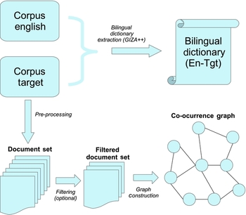
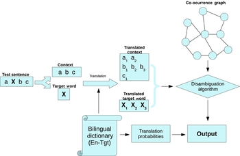
Figures 1 and 2 illustrate the complete system. Figure 1 shows the construction of two data structures used in our system: the bilingual dictionary and the co-occurrence graph. The bilingual dictionary is obtained from the original parallel corpus, both in the source language (always English) and in the target language (Spanish, French, Italian, German or Dutch). The corpus written in the target language is also taken as base for building the co-occurrence graph, after a pre-processing step and an optional filtering process. In Figure 2 we can observe how, given a test sentence, all the algorithms that we have explored for performing the final step in the disambiguation process, make use of the bilingual dictionary and the co-occurrence graph for providing an initial set of translations for the target word. This set is then combined with the translation probabilities extracted directly from the bilingual dictionary for generating the final output of the task. Each of the disambiguation algorithms, as well as the process of combining the initial output with the translation probabilities, will be explained later in this paper.
Construction of the bilingual dictionary and the co-occurrence graph.

Disambiguation process. Each of the analysed disambiguation algorithms makes use of the bilingual dictionary and the co-occurrence graph as sources of information for disambiguating each target word in each test sentence. ‘Tgt’ stands for ‘target’.

4 Bilingual dictionary extraction
We need to obtain bilingual dictionaries for all the proposed target languages, with English as the source language, in an automatic way. For this purpose, we use GIZA++ (Och and Ney Reference Och and Ney2003), an automatic tool that allows us to align at word level two parallel corpus, originally aligned at sentence level. The input of the GIZA++ tool consists of two files, each one of them representing a whole corpus written in a specific language. In these files raw text must be introduced, represented by one word per line, without XML tags or any other marks apart from the text to be aligned. We apply this tool over the sentence-aligned Europarl corpus of a pair of languages, and use the intersection of both translation directions. This way, we obtain bilingual dictionaries from English to German (En-De), from English to Spanish (En-Es), from English to French (En-Fr), from English to Italian (En-It), and from English to Dutch (En-Nl). It is important to remark that the GIZA++ tool provides information about the probability of occurrence of each translation of a target word. These translation probabilities, as we briefly explained in Section 3 and Figure 2, will be used as a prior probability for the translations provided by the bilingual dictionary. Specifically, this information given by GIZA++ will be combined with the initial output of the CO-Graph system for generating the final output for every test instance.
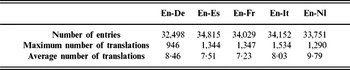
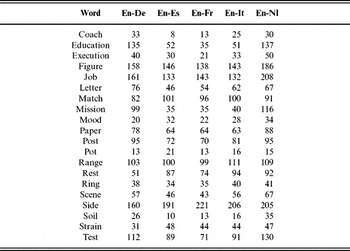
Tables 1 and 2 show some statistics extracted from the bilingual dictionaries obtained with the GIZA++ tool. Table 1 contains the number of entries of each dictionary, the maximum number of translations of a single entry, as well as the average number of translations per entry that can be found. Table 2 shows the number of translations provided by each of the bilingual dictionaries, for each target word in the test dataset of the SemEval 2010 and SemEval 2013 competitions.
Statistics from the bilingual dictionaries obtained through the GIZA++ tool, from English to German (column En-De), Spanish (column En-Es), French (column En-Fr), Italian (column En-It) and Dutch (column En-Nl)

Number of translations of the words in the test dataset, for each bilingual dictionary obtained through the GIZA++ tool

As we can observe in the tables, although the average number of translations per word is quite low, there exist words in the dictionaries that present a very large number of potential translations. In general, most of the target words in the test dataset present many translations, due to the automatic nature of the GIZA++ tool. We can then prune the dictionary and only consider those translations with highest probability. Some tests have shown that a pruning value of ten translations per word provides the best results. Hence, our system will have to select the most suitable translations for a given word in a given context, among a set of ten translations.
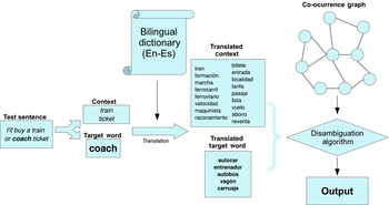
Figure 3 illustrates a specific example of the disambiguation process. In this case, we want to disambiguate the word ‘coach’ in a specific sentence, from English to Spanish. As we can observe, words surrounding the target words are considered as context. The bilingual dictionary provides the possible translations of the target word, as well as the translations of the words in the context. This information, together with the knowledge embedded in the co-occurrence graph, will allow us to perform the disambiguation, using one of the algorithms that will be explained later on.
Example of the disambiguation process of a sentence containing the target word ‘coach’, with Spanish as target language.

5 Knowledge representation
5.1 Corpus pre-processing
Although the Europarl parallel multilingual corpus, extracted from the proceedings of the European Parliament and taken as knowledge base for the task, is presented in many languages, only those proposed in the evaluation tasks are taken into account, namely English, Spanish, French, Italian, German and Dutch.
We split the initial corpus, divided in documents and XML-tagged, by detecting the interventions of different members of the Parliament. Each intervention, labelled with the ‘speaker’ tag, will become a document to be used later on by our algorithm. In this way, we intend to fulfil our hypothesis that the words appearing in the same document are likely to be related to the general sense of the document.
The words inside the documents need to be lemmatised and tagged according to their part-of-speech (POS) tag. The lemmatisation and POS tagging is automatically performed through the use of the TreeTagger tool (Schmid Reference Schmid1994).
5.2 Document filtering
We have considered two different ways of building the co-occurrence graph from the documents extracted from the original corpus. The first approach takes into account all the documents for building the graph, hence the same graph will be used for disambiguating any word from the test dataset. This approach will be denoted as ‘Complete graph approach’ along the rest of the paper. The second approach is based on the belief that more specific graphs will provide better results when performing the disambiguation. For this purpose, we build a specific graph for each of the target words appearing in the test dataset, by removing, from the original document set, those documents that do not contain any of the possible translations of the target word. Hence, we will obtain as many graphs as target words exist in the test dataset, and we will use, for each sentence, the graph that corresponds to the target word, for disambiguating it. This second approach will be denoted as ‘Word-based graph approach’ along the rest of the paper.
5.3 Co-occurrence graph construction
From the tagged documents in the target language, we are now able to build the co-occurrence graph that will allow us to perform the disambiguation. As we consider in our initial hypothesis, the appearance of a word in a document is likely to be related to the general sense of the document (intervention of a member), but not necessarily. Hence, in order to check if the co-occurrence of two words in the same document is statistically significant, a null model is defined, that represents what is considered pure chance. In this null model, words are randomly and independently distributed among a set of documents, and the probability of two words co-occurring by pure chance is calculated. If a co-occurrence can be easily (with high probability) generated by the null model, then it is not considered to be statistically significant. More specifically, a p-value p is calculated for the co-occurrence of two words inside the null model. If p ≪ 1 (lies below a given threshold next to 0), then the appearance of the two words in a document is significant (their meaning is probably related).
We consider two words w 1 and w 2 appearing in n 1 and n 2 number of documents respectively. In order to calculate in how many ways those two words could co-occur in exactly k documents, we can divide the complete set of documents in four different types of them: k documents containing both words at the same time, n 1 − k documents containing only word w 1, n 2 − k documents containing only word w 2, and N − n 1 − n 2 + k documents containing neither w 1 nor w 2, given that N is the total number of documents in the set. Thus, the number of possible combinations of co-occurrence is given by the multinomial coefficient:
 \begin{equation}
\binom{N}{k,n_1-k,n_2-k}=\binom{N}{k}\binom{N-k}{n_1-k}\binom{N-n_1}{n_2-k} .
\end{equation}
Then, given two words randomly and independently distributed among N documents, and appearing in n 1 and n 2 documents respectively, the probability of those words co-occurring in exactly k documents is given by:
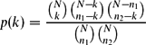 \begin{equation}
p(k)={\binom{N}{k}\binom{N-k}{n_1-k}\binom{N-n_1}{n_2-k}\over {\binom{N}{n_1}\binom{N}{n_2}}}
\end{equation}
if max {0, n 1 + n 2 − N} ⩽ k ⩽ min {n 1, n 2}, and zero otherwise.
Equation (2) can be rewritten in order to get an equivalent expression that is computationally easier to deal with. For this purpose, we introduce the notation (a)b ≡ a(a − 1). . .(a − b + 1), for any a ⩾ b, and without loss of generality, we assume that the first word, w 1, is the most frequent one, that is, n 1 ⩾ n 2 ⩾ k. Then:
 \begin{equation}
p(k) =\frac{(n_1)_k(n_2)_k(N-n_1)_{n_2-k}}{(N)_{n_2}(k)_k} = \frac{(n_1)_k(n_2)_k(N-n_1)_{n_2-k}}{(N)_{n_2-k}(N-n_2+k)_k(k)_k}
\end{equation}
where in the second form, the identity (a)b = (a)c(a − c)b − c, valid for a ⩾ b ⩾ c. Finally, Equation (3) can be rewritten as:
 \begin{equation}
p(k) =\, \prod _{j=0}^{n_2-k-1}\left(1-\frac{n_1}{N-j}\right) \times \prod _{j=0}^{k-1}\frac{(n_1-j)(n_2-j)}{(N-n_2+k-j)(k-j)}.
\end{equation}
This allows us to define the following a p-value p for the co-occurrence of two words:
 \begin{equation}
p=\sum _{k\ge r}p(k)
\end{equation}
where r is the number of documents in the corpus where both words have actually been found together. Now, if p ≪ 1, the co-occurrence of these particular two words is statistically significant, and then their meaning is likely to be related. Moreover, we can quantify this significance by taking the median (corresponding to p = 1/2) as a reference, and hence, a link will be established between both words inside the graph, its weight being ℓ = −log (2p), that is, a measurement of the deviation of r from the median.
6 Target word disambiguation
The construction of the co-occurrence graph gives us a structured representation of the knowledge inside the corpus. We now need to select from the graph those nodes closely related that can be considered to be related to the same sense. Although there exist many possible implementations of this step, in this work we will study three different techniques for determining the most suitable translations for a given word in a given context: Community detection, PageRank algorithm and Dijkstra’s algorithm.
6.1 Community detection and community graph
A community is a sub-graph whose nodes present some kind of structural or dynamic affinity. In this technique, we assume that words belonging to the same community share a common sense, different from those represented by other communities. There exist many different community extraction algorithms. In this work, we use two algorithms, and compare their results:
• Walktrap: The Walktrap algorithm (Pons and Latapy Reference Pons and Latapy2005) is based on the fact that a random walker that jumps between nodes inside the graph, will get more easily trapped in those sub-graphs that are densely connected. These sub-graphs would then become the communities.
• Chinese whispers: The Chinese whispers algorithm (Biemann Reference Biemann2006) is a simple yet efficient technique that assigns each vertex to a community in a bottom-up fashion. In the first step, the algorithm assigns a distinct class to each vertex. Then, the nodes are iteratively assigned to the class that contains the strongest neighbours of the analysed node (those with highest weights in edges linked to the current node).
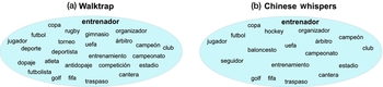
Figure 4 shows an example of the differences between communities when using both algorithms. We have selected the word ‘entrenador’ in Spanish, which is a translation of the word ‘coach’, referred to a person that trains an athlete or team. As we hypothesised, words in the communities tend to be related to this particular sense of the word ‘coach’, such as ‘futbol’ (‘football’ or ‘soccer’), ‘golf’, ‘rugby’, ‘entrenamiento’ (‘training session’), ‘arbitro’ (‘referee’), ‘jugador’ (‘player’), ‘estadio’ (‘stadium’), ‘campeonato’ (‘championship’). As we can observe, both algorithms generate a similar community, although the one provided by the Chinese whispers algorithm is smaller.
Communities containing the word ‘entrenador’ as translation of ‘coach’ in Spanish: (a) Walktrap algorithm; (b) Chinese whispers algorithm.

With the communities obtained by the algorithm, we build a new graph, called community graph (CG). In this graph, each community is represented by a node, and an edge will be added linking communities (nodes) C 1 and C 2 if and only if any word x ∈ C 1 is linked in the co-occurrence graph to any word y ∈ C 2.
Context surrounding the target word is the only additional information that can be used to perform the disambiguation. In this case the co-occurrence graph has been built using only nouns, thus can eliminate all the remaining words (adjectives, verbs, . . .) from the context.
The next step is to identify, inside the community graph CG, those communities that contain at least one of the translations, either from words of the context or from the target word. As a result, we obtain two sets of communities: set MT includes communities that contain at least one translation from the target word, and set MC is composed by communities containing at least one translation from any word of the context. Through the community graph we can calculate the distances between any community MiC ∈ MC and any community MjT ∈ MT. Since a translation of a target word can belong to the same community that a translation of a context word (MiC = MT j), the distance in that case would be 1, which is the minimum distance we consider. In any other case, we will add the number of links in the shortest path between MiC and MjT. Hence, if the path between MiC and MjT contains one link, the distance between them, for our purposes, would be 2, if the path contains 2 links, the distance would be 3, and so on.
Our hypothesis for this algorithm is that the translation of the target word that is nearer (in average) to the translations of the context words, is more likely to be the most suitable translation for that target word in that context. Hence, we establish a formula for ranking the potential translations of the target word, based on two factors: the score of a translation is inversely proportional to the distance between the community to which it belongs and any community containing context translations, in order to give greater emphasis to first-order co-occurrences (Schütze Reference Schütze1998), but directly proportional to the number of context translations inside the community. Thus, the weight or score of a translation of the target word, wt, will be given by:
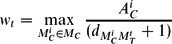 \begin{equation}
w_t = \max _{M_C^i \in M_C}{{A_C^i} \over (d_{{M_C^i}{M_T^t}} + 1)}
\end{equation}
where AiC is the number of context translations inside MiC, and d MiCMtT is the distance (number of steps) between MiC and MtT, that is, the community in which translation t is located. By ranking the scores of all the possible translations for the target word given by the dictionary, the system can propose the most suitable ones as a solution.
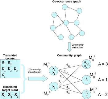
Figure 5 illustrates the algorithm based on communities and contains an example of its behaviour, as explained above. In the example, links between nodes of the community graph do not necessarily represent paths containing one only link, but any possible value of d i, j. Hence, in that example word X 1 will have a weight  $w_1=\max {({3 \over d_{1,1}+1}, {1 \over d_{1,2}+1}, {2 \over d_{1,3}+1})}$. Word X 2 will have the same weight, w 2 = w 1, since X 1 and X 2 belong to the same community. Finally, word X 3 will have a weight
 $w_1=\max {({3 \over d_{2,1}+1}, {1 \over d_{2,2}+1}, {2 \over d_{2,3}+1})}$.
Diagram and example of the community-based algorithm. The community graph is extracted from the co-occurrence graph, and used to compute the distances between words from the context and the target word.

6.2 PageRank algorithm
The PageRank algorithm (Brin and Page Reference Brin and Page1998) is used over a graph for ranking the importance of each of its nodes. This algorithm has been widely used in the last years for performing WSD (Mihalcea Reference Mihalcea2005; Agirre and Soroa Reference Agirre and Soroa2009; Navigli and Lapata Reference Navigli and Lapata2010). The PageRank calculation for the whole graph can be performed through the following formula:
 \begin{equation}
P = dMP + (1-d)v
\end{equation}
P is a vector with the PageRank values for each node, d is a constant called ‘damping factor’ and usually set to 0.85, M is the matrix representing the outdegrees of the nodes, and v is a N × 1 stochastic vector, being N the number of nodes in the graph. By means of v, the probability of randomly jumping into a node of the graph can be distributed among the nodes of the graph in different ways. In this work, we will explore two approaches for applying the PageRank algorithm:
• Basic PageRank: All the members of vector v will have the same value,
 $v_i={1\over N}$. Therefore, in this approach the context of the sentence in which the target word appears is not taken into account.
• PageRank with Priors: In this case, the vector v will be used for giving more importance to those words surrounding the target word in a specific context, in a similar way to that explained in (Agirre, Lopez de Lacalle and Soroa Reference Agirre, Lopez de Lacalle and Soroa2014). If there are C words in the translated context of a specific sentence, the values of members of vector v will be
$v_i={1\over C}$ if node i represents the translation of a word of the context, and 0 otherwise.


Once that we have calculated the PageRank (either basic or with Priors) of our co-occurrence graph, we can determine the most suitable translations of a target word by simply selecting those translations with higher values of PageRank.
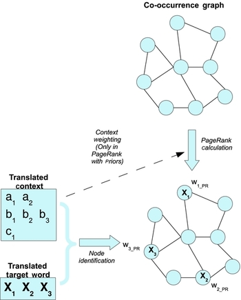
Figure 6 shows the behaviour of the PageRank algorithm for disambiguation. The translations of the target word are sought inside the graph, and their weights will correspond to those assigned by PageRank, w 1 = w 1_PR, w 2 = w 2_PR and w 3 = w 3_PR.
Diagram and example of the PageRank algorithm. The translation of the context is used only if we are performing the ‘PageRank with Priors’ approach.

6.3 Dijkstra’s algorithm
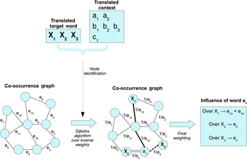
The shortest path from node i to node j of a graph can be calculated through Dijkstra’s algorithm (Dijkstra Reference Dijkstra1959), which uses weights of the links for selecting a path. Through this algorithm, we can calculate the shortest distance between the translation of a word of the context, and a translation of a target word, and use this information for ranking those translations. Since weights in the graph represent the importance of a link between two words, we will assign, for each link, the inverse of its original weight for obtaining the minimum distances.
For assigning a value to the influence that a context word has in the selection of a particular translation of the target word, we retrieve the original weights (representing the importance of a link between two words) of the links in the graph and sum all the values of the edges involved in the shortest path. Then, this final sum is divided by the number of edges in the path. Hence, for each translation of each context word, tc, and each translation of the target word, tw, we obtain a value related to the shortest path between those words in the original graph. Then, the score of each possible translation of the target word will be the highest weight that is assigned in this step, this is, the highest influence given by a context word. By ranking these values, we can determine the most suitable translations for the target word given a specific context.
Figure 7 shows the different steps of the technique based on Dijkstra’s algorithm, and an example of its behaviour. Dijkstra’s algorithm is applied to the co-occurrence graph. Following the above description of the algorithm, if we represent the influence of a translation of a context word, tc, over a translation of the target word, tw, in terms of a function I(tc, tw), we obtain that  $I(a_1, X_1) = {{e_{10} + e_{13}}\over 2}$, I(a 1, X 2) = e 5 and I(a 1, X 3) = e 4. Hence, considering the translations of context words shown in the example of the figure, the weight of any translation of the target word Xn will be wn = max (I(a 1, Xn), I(a 2, Xn), I(b 1, Xn), I(b 2, Xn), I(b 3, Xn), I(c 1, Xn)).
Diagram and example of the technique based on Dijkstra’s algorithm. The weights of the edges in the co-occurrence graph are inverted for computing the shortest path algorithm. The different lines in the edges after applying Dijkstra’s algorithm represent the shortest paths from a 1 to X 1 (continuous line), X 2 (double line) and X 3 (dashed line) respectively.

6.4 Output of the system
GIZA++ provides very valuable information about the translations, and it has a different nature than the weights our system assigns to each potential translation. This information is also obtained in an automatic, unsupervised way. This suggests combining the weights obtained by our system, through any of the disambiguation algorithms, with the most probable translations of a target word. Accordingly, we will assign a final score to each of the ten potential translations provided by the dictionary. This final score will be extracted by multiplying the score obtained by the CO-Graph system, and the probability of translation given by GIZA++. This is, we consider T = (t 1, t 2, . . ., tn) to be the complete set of potential translations provided by GIZA++ for a given target word, where n < =10. Each translation ti has an associated probability pi. After applying the disambiguation process, the CO-Graph system assigns a weight wi to each of the potential translations. The final score of each translation si will be given by si = piwi. In the following experiments we will illustrate the results obtained by applying this combination of the weights of the system and the probabilities of translation. Besides, we will also show results obtained by only using the CO-Graph system, without using this prior probability or backoff given by GIZA++.
7 Evaluation
7.1 Evaluation criteria
The evaluation setting followed in our experiments is based on the one proposed in task 3 of SemEval 2010 and task 10 of SemEval 2013 competitions. The disambiguation is performed taking English as the source language, and five different languages as target languages, namely Spanish, French, Italian, Dutch and German. Systems participating in the tasks are asked to propose the most suitable translations for each test sentence in as many languages as possible. Evaluation is carried out, in both tasks, over a test dataset with 20 different words and 50 sentences for each of them, and results are compared against a manually built gold standard containing the most suitable translations for each target word in each sentence.
The gold standard is built from the Europarl corpus. For this purpose, a word-level alignment was performed and manually evaluated for all the sentences of the corpus containing target words, for every pair of languages containing English as the source language. After that, a manual clustering by meaning was carried out, for every target word. The output of this process was a sense inventory, used for annotating the datasets for the tasks (Lefever and Hoste Reference Lefever and Hoste2010b).
Annotators of the gold standard used the clustered sense inventory for selecting the most appropriate translations of each target word. The translations are weighted depending on how many annotators selected each of them. Example 7.1 shows the gold standard provided by the annotators for a given sentence in which we can find the target word ‘ coach’.
(8) SENTENCE 2: A branch line train took us to Aubagne, where a coach picked us up for the journey up to the camp.
coach.n.nl 2 :: bus 3; autobus 3; toerbus 1; touring car 1;
coach.n.fr 2 :: bus 3; autobus 3; car 3;
coach.n.de 2 :: Bus 3; Omnibus 2; Reisebus 2; Linienbus 1; Reisebus 1;
coach.n.it 2 :: autobus 3; pullman 2; corriera 2; autocarro 1; pulmino 1;
coach.n.es 2 :: autocar 3; autobus 3; diligencia 1;
Two different evaluation schemes are proposed:
• Best evaluation: The first evaluation scheme asks the systems to propose any number of translations for each target word in each context, but the final score is divided by the number of translations. Hence, the scoring process penalises the systems proposing too many translations. In our case, we consider only those translations (up to two), among the ten potential translations provided by the bilingual dictionary, whose normalised weight (between 0 and 1), is higher than 0.3 (30% of the total weight). If there are no translations that fulfil this condition, only the translation with the highest weight is proposed, except if there exists a tie. In that case, the two translations with the highest weights are considered.
• Out-Of-Five evaluation: This ‘more relaxed’ scheme expects an output of up to five different translations for each target word in each context, without penalising the system according to the number of translations. Hence, given that the dictionary constrains the number of translations of each word to ten, our system will have to select, in any of the proposed disambiguation algorithms, five of those potential translations as a solution for each test instance.
The evaluation measure considered in these tasks is F-measure. Due to the nature of the guessings proposed by our system, the values of precision and recall (and hence the value of F-measure) are always the same. Then, we will refer only to the F-measure value for illustrating the results achieved by our system, and for comparing them with other systems participating in the SemEval competitions.
7.2 Experimental results
The co-occurrence graph is built using only nouns as nodes, since nouns are considered the most informative elements in the sentences. When the graph is constructed, a threshold for the p-value p has to be set, in order to indicate the highest value of p for which the number of co-occurrences of two words is considered to be statistically significant and therefore a link is created between them. As this threshold decreases, the graph becomes more restrictive, and hence the number of edges also decreases. In this work, we have used the trial dataset provided in the SemEval 2010 competition for analysing the influence of the threshold in an exhaustive way. Then, based on those results we will select a specific threshold for performing the experiments in all the languages and all the tested algorithms, on the 2010 and 2013 test datasets.
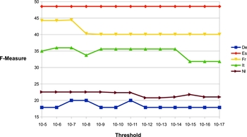
Figure 8 shows the evolution of the behaviour of the system as we decrease the threshold for building the graph, from p = 10−5 to p = 10−17.
Evolution of the F-measure achieved in a single experiment, as the threshold decreases (graph becomes more restrictive). Results for the PageRank algorithm in the ‘Complete graph approach’ using the trial dataset of the 2010 SemEval competition.

As we can observe in the figure, for all the languages best results are achieved with values of the threshold between p = 10−5 and p = 10−11, while smaller thresholds lead to a decrease of the performance of the algorithm. Within this smaller range of thresholds, the F-measure values are quite similar. This can be observed in most of the experiments conducted in this work, hence selecting any value of the threshold in that range would provide similar results. Specifically, we have selected a threshold value of p = 10−6 for all the experiments in this section, given any language or algorithm. This way, we want to test the robustness of our system under the same conditions that the systems participating in the SemEval competitions.
7.2.1 Baseline: most frequent sense
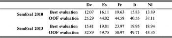
As we stated above, GIZA++ not only generates a dictionary from a language to another in an automatic way, but it also provides the probability of each translation of each word. Hence, the use of GIZA++ for creating the bilingual dictionaries allows us to generate a baseline to which compare our system: the most probable translations (most frequent sense or MFS). As we are considering two different evaluation schemes, we will provide the most probable translation for the ‘Best Evaluation’ scheme, and the five most probable translations for the ‘Out-Of-Five Evaluation’ scheme. Table 3 illustrates the results offered by a MFS approach applied to the 2010 and 2013 SemEval test datasets. Both evaluation schemes (‘Best’ and ‘Out-Of-Five’) are shown in the table.
MFS Baseline. Results (F-measure in %) obtained by a MFS approach for the best and out-of-five (OOF) evaluation schemes in the SemEval 2010 and SemEval 2013 competitions

As expected, the results for the ‘Best’ evaluation scheme are always lower than those for the more relaxed ‘Out-Of-Five’ scheme. In general, Spanish, French and Italian obtain better results than Dutch and German, and this trend will be repeated along all the experiments performed with our system, and also along the results offered by different systems participating in the competitions. The fact that Dutch and German are languages for which disambiguation is a more difficult task, can be caused by the higher number of translations, in general, that they present for each target word, as we observed in Table 2. It is important to state that this baseline based on most frequent senses is usually hard to overcome by systems participating in CLWSD tasks. Actually, the baselines proposed by the organisers of the 2010 and 2013 competitions, which were also based on a MFS approach, were not surpassed by many of the participating systems, even supervised ones. Moreover, when the baselines were outperformed, the differences were small. This fact will be shown in the following sections containing results from the best systems participating in the competitions.
7.2.2 Word-based graphs versus complete graphs
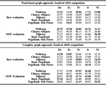
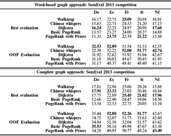
In this section, we present the results obtained by our system, using the approaches briefly described in Section 5.2, this is, word-based graphs and complete graphs, and we compare both techniques. Table 4 shows the results for the word-based graph and complete graph approaches in the SemEval 2010 test dataset, and Table 5 shows the results obtained by both approaches in the SemEval 2013 test dataset. All the algorithms described in Section 6 are tested and compared. Results shown correspond to the F-measure value.
Results (F-measure in %) obtained by the word-based graph and complete graph approaches of the CO-Graph system for the best and out-of-five (OOF) evaluation schemes in the SemEval 2010 competition. Results for the five different disambiguation algorithms are presented, for the five languages involved in the task. Bold highlights the algorithm that reach the best results for each approach, language and evaluation scheme

Results (F-measure in %) obtained by the word-based graph and complete graph approaches of the CO-Graph system for the best and out-of-five (OOF) evaluation schemes in the SemEval 2013 competition. Results for the five different disambiguation algorithms are presented, for the five languages involved in the task. Bold highlights the algorithm that reach the best results for each approach, language and evaluation scheme

Regarding the different disambiguation algorithms, as we can observe in the tables, in general the techniques based on the Walktrap algorithm and on Dijkstra’s algorithm show the best results, both for the ‘Best’ and the ‘Out-Of-Five’ evaluation schemes. There are some cases in which the other community-based algorithm, Chinese whispers, slightly outperforms those results. However, in those cases, the improvement with respect to the second best result is really small. Also, the PageRank with Priors algorithm, and the Basic PageRank algorithm obtain the best result for some of the experiments. In these cases, the improvement is also not significant. Hence, we can assume that the algorithms based on distances and paths between translations of words from the context and potential translations of the target word (community-based and Dijkstra) perform better than those based only on the outdegree of the nodes and random jumps (PageRank). The community-based algorithms take into account the weights of the links in the co-occurrence graph for extracting the communities, while Dijkstra’s algorithm considers them (their inverse) for obtaining the shortest path between two nodes. Therefore, an accurate weighting of the connections of the nodes in the graph is important for obtaining good results.
The comparison between the word-based graph and the complete graph approaches shows a general trend in which the results obtained by the complete graph approach are better than those provided by the word-based graph approach, although most of the improvements are small. This can be due to the greater completeness of the general graph used for disambiguation, that takes into account not only information about the target word, but about the structure of the corpus in a more generalistic way. Specifically, in German, Spanish and French this improvement is clear. Accordingly, and considering that a unique graph for disambiguating all the target words is better in terms of efficiency, we will select the complete graph approach and the technique based on Dijkstra’s algorithm for the rest of the evaluation, and for the comparison with other state-of-the-art systems.
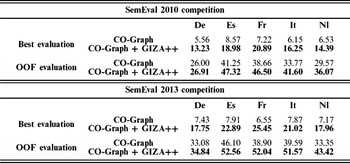
Once that we have selected a particular threshold value and a particular technique for building the graphs and performing the disambiguation, we want to compare its results with those obtained by the same technique (Dijkstra’s algorithm with complete graphs and a threshold value of 10−6), but without the combination with the translation probabilities given by GIZA++. We examine the performance of the CO-Graph system alone, and determine if the combination proposed in Section 6.4 improves the original results. Table 6 shows this comparison.
Comparison of results (F-measure in %) for the selected configuration of the system (threshold value p = 10−6, Dijkstra’s algorithm, complete graph approach), between the CO-Graph system alone and the CO-Graph system combined with the prior translation probabilities given by GIZA++, for the 2010 and 2013 test datasets, in both the ‘Best’ and ‘Out-Of-Five’ evaluation schemes. Bold highlights the technique that reaches the best results

The table clearly shows that the original CO-Graph system is substantially improved by combining its output with the translation probabilities given by GIZA++. Specifically, results for the ‘Best’ evaluation scheme present the highest improvements. This suggests the importance of the backoff provided by the most frequent sense of a given target word for selecting only the most suitable translations. In the ‘Out-Of-Five’ scheme, important improvements are also achieved in most of the languages. This confirms our hypothesis about the benefits derived from the use of the prior translation probabilities given by the bilingual dictionaries, suggested in Section 6.4. Nevertheless, the results obtained by CO-Graph alone are still competitive, specifically in some cases of the ‘Out-Of-Five’ evaluation. The system that combines the CO-Graph weights and the translation probabilities will be used along the rest of the paper for performing comparisons with other state-of-the-art systems.
7.3 Comparative
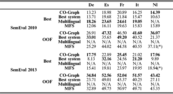
In this section, we compare (Table 7) our system with the best unsupervised systems participating in the SemEval 2010 and 2013 competitions, briefly described in Section 2.1. The MFS baseline proposed in Section 7.2.1 is also included in the table for comparison. Also, the multilingual system described in Navigli and Ponzetto (Reference Navigli and Ponzetto2012) is compared separately, since it did not participate in the competitions, and only proposes results for the ‘Best’ evaluation scheme of the SemEval 2010 test dataset.
Comparative of the results (F-measure in %) obtained by the CO-Graph system, the unsupervised systems obtaining the best results, and the MFS approach, for the SemEval 2010 and SemEval 2013 competitions, in the five proposed languages. Bold highlights the best system (CO-Graph, best unsupervised or multilingual approach), and asterisk (*) indicates the cases in which the CO-Graph system has not been able to overcome the MFS approach
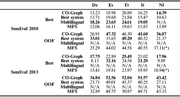
The table shows that the CO-Graph system overcomes the best unsupervised systems that participated in the SemEval competitions in most of the cases (13 out of 20). The multilingual system, although it did not participate in the competitions, outperforms our system and the best unsupervised systems in all the cases for which it proposes results (‘Best’ scheme for German, Spanish, French and Italian). However, although unsupervised, this system uses external resources such as BabelNet (Navigli and Ponzetto Reference Navigli and Ponzetto2010) and WordNet (Fellbaum Reference Fellbaum1998) for performing the disambiguation, while our system only makes use of a parallel corpus for extracting the knowledge. In general, our system performs better for the ‘Out-Of-Five’ evaluation scheme, compared to the ‘Best’ evaluation, and also for the 2013 test dataset, compared to the 2010 dataset. In the 2013 edition, all the unsupervised systems are surpassed in the ‘Out-Of-Five’ scheme, and only one of them, called NRC-SMT (Carpuat Reference Carpuat2013), clearly overcomes our system in the ‘Best’ scheme, for the Spanish language. This system is focused on the Spanish language only, so its coverage of the problem is lower than ours. In the Italian language, a system, called LIMSI (Apidianaki Reference Apidianaki2013) obtains slightly better results than ours, but the difference is so small (an improvement of 0.18%), that it can be considered as a tie. The system that overcomes ours in the ‘Out-Of-Five’ scheme of the 2010 dataset (German and French) is called T3-COLEUR (Guo and Diab Reference Guo and Diab2010). Although it is an unsupervised system, it takes additional information from some external resources, since WordNet synsets are used to augment the translation correspondences and yield more translation variability.
Our system is able to overcome the MFS approach in most of the cases. Only in two of the 20 cases the MFS approach presents better results, but the differences are really small (around 1%).
7.4 Example of disambiguation
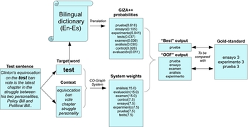
In this section, we present two examples of the disambiguation process for a given word in a given context (test sentence). Since the creation of the co-occurrence graph cannot be illustrated in an example due to its size, only the disambiguation step is shown, after the generation of the co-occurrence graph. The technique illustrated in these examples is the community-based algorithm, and the language is Spanish. Both evaluation schemes are presented and the results offered by the CO-Graph system can be compared to the gold standard for the same test sentences. Figures 9 and 10 show the disambiguation in Spanish of the target word ‘ test ’ and ‘ strain ’, respectively, each of them inside a test sentence.
Example of disambiguation. The target word is ‘ test ’ and the final language is Spanish.

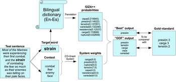
Example of disambiguation. The target word is ‘ strain ’ and the final language is Spanish.

The target word and the context are separated from the original sentence, and introduced as an input to the CO-Graph system. The system uses the bilingual dictionary and the co-occurrence graph, as well as the community-based technique, for extracting the weights for disambiguation. At the same time, the translation probabilities are obtained from the bilingual dictionary. The final scores are obtained and ranked according to the scoring process stated in Section 6.4. Hence, we obtain the final translations for the ‘Best’ and ‘Out-Of-Five’ evaluation schemes. This will be compared against the gold standard for evaluating the disambiguation.
In the first example, we observe that the CO-Graph system assigns two different values (15.0 and 7.5) to the possible translations before using the translation probabilities given by GIZA++. According to those values, the words in the gold standard are not among those with highest weights. However, those words in the gold standard happen to be among the most probable translations of the GIZA++ dictionary, and when the combination between both values is performed, the correct translations (‘ensayo’, ‘experimento’ and ‘prueba’), appear in the final output of the system. Hence, the solution given for this particular case is successful, although it represents an example of the case in which most of the useful information comes from the translation probabilities given by GIZA++.
In the second example, we can also observe a case in which a successful solution is achieved. In this case, the CO-Graph system alone is able to propose most of the correct translations for the target word in the test sentence. Words ‘presion’ and ‘carga’, present in the gold standard, obtain the highest weights from the CO-Graph system alone. The translation with highest probability according to GIZA++ (‘cepa’) is not among those contained in the gold standard. This word has a small weight in the CO-Graph system ranking, and hence when the combination of weights is performed to obtain the final output, this word does not get a high value in the final ranking. Accordingly, a possible decrease of the performance, that could be caused by given too much importance to that word, is avoided thanks to the weights given by the CO-Graph system alone. Apart from this, the effect of the translation probabilities can be seen for the word ‘tension’, which obtains a slightly smaller CO-Graph weight, and thanks to the translation probability given by GIZA++ is proposed to be the second most probable translation in the final solution.
8 Conclusions and future work
In this work, we have presented an approach to perform CLWSD, based on the construction of a co-occurrence graph containing the knowledge of a corpus. We have shown the validity of the new unsupervised graph-based technique, which uses the whole document as a coherent piece of information, while other works consider windows of a specific size for building the context and calculating the co-occurrences. The results obtained support our hypothesis about the effectiveness of the approach. Results also shown that algorithms based on the weights of the links in the co-occurrence graph (community-based techniques and Dijkstra’s algorithm) performs slightly better on average that the other proposed techniques. The community-based techniques use the weights of the links in the co-occurrence graph for extracting the communities, and the technique based on Dijkstra’s algorithm takes those same weights into account for finding the shortest paths between nodes. The results indicate that the weights assigned to the links in the co-occurrence graph construction process are useful for determining the influence of surrounding words on the target word. However, the differences between those algorithms and the algorithms based on the relative importance of each node in the graph (PageRank, in its different variants), are not very large.
We have shown the relevance of considering the probabilities of occurrence of the different translations taken into account for a target word, through the combination of weights proposed by the system and the values of these translation probabilities. The conclusion that can be drawn from this fact is that information regarding the possible translations of the target words (which can be obtained in an automatic, unsupervised way), is a key knowledge for systems performing CLWSD, and hence a bilingual dictionary offering this kind of information is very important for building competitive systems.
The results also show that our system is among the best unsupervised systems that participated in those competitions, overcoming all of those systems for some languages, and obtaining the second best results for some others. In general, we can observe that the results of the ‘Out-Of-Five’ evaluation scheme are better than those achieved using the ‘Best’ evaluation scheme. In fact, our system overcomes all the participating unsupervised systems in the SemEval 2013 competition, for the ‘Out-Of-Five’ evaluation scheme. The difference of performance for the two evaluation schemes may be due to the fact that the ‘Best’ evaluation requires more pronounced differences among the weights. This could be achieved by increasing the influence of the context. One could also expect larger differences between the results of the basic PageRank and the PageRank with Priors, which takes the context into account, than those obtained in our experiments. Regarding those facts and suggestions, more work needs to be done in refining the algorithms used for selecting the most suitable translations proposed by the dictionary, increasing the influence of words of the context.
It is also important to indicate that those unsupervised systems that overcome our results make use of some additional external resources, or are focused only on one language, as we stated above, while our system only use the proposed corpus for extracting knowledge, and provides good results for all the languages proposed in the tasks. Hence, we can conclude that the performance of the system is better than that presented by other unsupervised systems using the same resources. Our system also presents a remarkable robustness and coverage of the problem.
Regarding the considered languages, the best results are obtained for Spanish, French and Italian, while the lowest ones correspond to German, which has been proved to be a more difficult task to solve in both competitions for all the participating systems. The combination of the output of the system and the most probable translations provided by the dictionary overcomes the results obtained by the baseline (MFS approach) in most of the cases. As it can be seen in the results of the 2010 and 2013 competitions (even for supervised systems), the fact of outperforming the MFS approach is not a small achievement, as this kind of baselines are usually hard to overcome in CLWSD tasks. In general, we can point out the robustness achieved by our system, with respect to parameters (such as the p-value) and languages.
Future lines of work rely on using weights in the co-occurrence graph not only for Dijkstra’s algorithm or for building the communities in the community-based technique, but also for PageRank. This can provide some additional information that improves the results. Considering translations containing more than one word (multi-word translations) is a necessary step for next versions of the algorithm. Specifically, an analysis of the gold standards used for evaluation indicates that in average, 3.26% of the expected translations are composed by more than one word. This value varies depending on the language (0.10% for German, 4.22% for Spanish, 1.75% for French, 8.50% for Italian and 2.36% for Dutch), so the potential improvement that can be achieved by incorporating these multi-word translations will also vary. Another line of work is to test our system on different datasets and sources of knowledge. Also, we want to analyse the influence of including other types of words such as adjectives or verbs in the co-occurrence graphs. Finally, scenarios where domain exists change across documents, and even tasks in which parallel corpora are not available as a source of information should be studied, in order to perform a deeper analysis of the performance of the CO-Graph system alone, without considering translation probabilities.
Acknowledgements
This work has been partially supported by the Spanish Ministry of Science and Innovation within the project EXTRECM (TIN2013-46616-C2-2-R), and the Universidad Nacional de Educación a Distancia (UNED) (2013-025-UNED-PROY).