1 Introduction and objectives
This study examines the turbulent boundary layer affected by sweep – that is, by misalignment between the pressure gradient and the free-stream velocity vector. The result is a three-dimensional boundary layer (3DBL), which is characterized by mean velocities and vorticities that change direction as well as magnitude with distance from the surface. The pressure-driven Ekman layer is a prototype, for the horizontally homogeneous case. Here we consider the non-homogeneous, spatially developing, incompressible turbulent 3DBL over an idealized (flat, smooth)
 $35^{\circ }$
infinite swept wing. The spatial development is due to a prolonged adverse (APG) then favourable (FPG) pressure gradient in the ‘chordwise’ direction (normal to the leading edge), applied to a two-dimensional (2-D) mean state with non-zero spanwise (parallel to the leading edge) mean velocity. Note that this use of ‘spanwise’ and ‘chordwise’ is not uniform aeronautical terminology, since these sometimes indicate directions respectively normal and parallel to the direction of flight (cf. Bradshaw & Pontikos Reference Bradshaw and Pontikos1985); the direction of flight itself will be referred to here as ‘streamwise’.
This paper has many references to the ‘collateral’ boundary layer. Following Driver & Johnston (Reference Driver and Johnson1990), we use this term to describe a 2-D boundary layer – such as the initial/inflow 2-D state just mentioned – whose non-zero spanwise component of mean velocity is solely an artefact of the orientation of the coordinate system.
Direct numerical simulation (DNS) is used to create a computational counterpart of the infinite-swept-wing experiments of Bradshaw & Pontikos (Reference Bradshaw and Pontikos1985) and especially, since it also involves separation, of van den Berg et al. (Reference van den Berg, Elsenaar, Lindhout and Wesseling1975). This study continues and generalizes our work on unswept turbulent separation bubbles, presented in Coleman, Rumsey & Spalart (Reference Coleman, Rumsey and Spalart2018, henceforth denoted CRS18). Interest in this flow is motivated by the importance of, and modelling challenge posed by, turbulent smooth-body separation (Slotnick et al.
Reference Slotnick, Khodadoust, Alanso, Darmofal, Gropp, Lurie and Mavriplis2014), coupled with the observation that pressure-induced separation of a turbulent 3DBL, where an APG causes reversal of the surface shear stress in a direction not aligned with the free-stream velocity, is quite common. The aim is to determine how this type of separation compares to that of the unswept counterpart, in particular how similar the mean-velocity field of the unswept flow is to the chordwise-component field of the swept version. In other words, is the projection of the swept flow onto the (chordwise–wall-normal) plane in which the gradients act identical, or close, to a two-dimensional turbulent flow with the same boundary conditions? This naturally leads to the question of the validity of the ‘Independence Principle’ (IP) for turbulent infinite-swept-wing boundary layers. Recall that for the laminar layer the IP is exactly satisfied, since the chordwise component is independent of the spanwise velocity component, as a consequence of the zero derivatives in the spanwise direction (Prandtl Reference Prandtl1945; White Reference White1991; McLean Reference McLean2013). For the turbulent case, we interpret the IP as requiring the mean chordwise and vertical components
 $(\bar{u},\bar{v})$
be unaffected by the mean spanwise component
 $\bar{w}$
. In particular, for given chordwise boundary conditions, the
 $(\bar{u},\bar{v})$
solutions for finite and zero
 $\bar{w}$
are equivalent. Consequently, the above question regarding the characteristics of the chordwise projection and the question of the validity of the IP are the same. (See Wygnanski, Tewes & Tauber (Reference Wygnanski, Tewes and Tauber2014) for an alternative interpretation of the IP, which focuses on the behaviour of the vector sum instead of the individual
 $\bar{u},\bar{w}$
components.)
That turbulence can invalidate the IP is revealed by consideration of the standard 2-D ZPG collateral layer over the infinite swept wing. We assume that the mean flow all the way across the boundary layer is in the direction of the flow outside the boundary layer, and obeys the standard log law. The failure of the IP for this flow is evidenced by the deviation from the logarithmic law for the chordwise component, written in terms of its wall-friction velocity
 $u_{\unicode[STIX]{x1D70F}_{x}}=\sqrt{\unicode[STIX]{x1D70F}_{w_{x}}/\unicode[STIX]{x1D70C}}$
: because the chordwise wall stress is
 $\unicode[STIX]{x1D70F}_{w_{x}}=\unicode[STIX]{x1D70F}_{w_{tot}}\cos \unicode[STIX]{x1D70E}$
, where
 $\unicode[STIX]{x1D70F}_{w_{tot}}$
is the total wall shear stress, and
 $\unicode[STIX]{x1D70E}$
the sweep angle, the effective von Kármán constant for the chordwise velocity is
 $\unicode[STIX]{x1D705}_{x}=\unicode[STIX]{x1D705}/\sqrt{\cos \unicode[STIX]{x1D70E}}$
, while the additive constant is
 $A_{x}=A\sqrt{\cos \unicode[STIX]{x1D70E}}-\ln (\cos \unicode[STIX]{x1D70E})/2\unicode[STIX]{x1D705}_{x}$
, where
 $\unicode[STIX]{x1D705}$
and
 $A$
are the standard 2-D/ZPG values. (This follows from the
 $x$
-component log law,
 $\bar{u}/u_{\unicode[STIX]{x1D70F}_{x}}=(1/\unicode[STIX]{x1D705}_{x})\ln (yu_{\unicode[STIX]{x1D70F}_{x}}/\unicode[STIX]{x1D708})+A_{x}$
, which for the collateral flow can be written
 $\bar{q}\sqrt{\cos \unicode[STIX]{x1D70E}}/u_{\unicode[STIX]{x1D70F}}=(1/\unicode[STIX]{x1D705}_{x})\ln (yu_{\unicode[STIX]{x1D70F}}/\unicode[STIX]{x1D708})+(1/\unicode[STIX]{x1D705}_{x})\ln \sqrt{\cos \unicode[STIX]{x1D70E}}+A_{x}$
, where
 $\bar{q}^{2}=\bar{u}^{2}+\bar{w}^{2}$
.) Physically, the increased value of
 $\unicode[STIX]{x1D705}_{x}$
reflects the higher intensity of the turbulence, itself driven by the larger shear rates of the total flow, compared with
 $\unicode[STIX]{x2202}\bar{u}/\unicode[STIX]{x2202}y$
(cf. p. 158 of Schubauer & Tchen Reference Schubauer, Tchen and Lin1959). Since the log-law deviation is a function of the sweep angle, the chordwise velocity
 $\bar{u}(x,y)$
is not set solely by its free-stream boundary condition
 $U_{\infty }=Q_{\infty }\cos \unicode[STIX]{x1D70E}$
, where
 $Q_{\infty }$
is the free-stream velocity magnitude, and is thus not independent of the spanwise flow
 $\bar{w}(x,y)$
. This behaviour, which in itself implies the failure of the IP in the ZPG layer, will be fully confirmed by the DNS results (§ 3.1).
Because the fully turbulent swept-wing flow studied here will contain ZPG regions, we do not expect the IP to be valid at all locations. On the other hand, since it will also include a strong APG, which exceeds the turbulent-stress gradients and eventually leads to mean separation (chordwise flow reversal), the flow may be characterized by zones in which the IP is a useful approximation (since the IP also applies to inviscid flow, not just laminar flow). This, in fact, will turn out to be the case.
A practical question is whether the presence of sweep increases, decreases, or has no effect upon the accuracy of separation predictions given by Reynolds-averaged Navier–Stokes (RANS) models. Since the breakdown of the IP for the collateral ZPG case will presumably not be overtaxing, and since for a swept-wing boundary layer the magnitude of the total wall shear stress at the separation line is finite, one might anticipate the presence of sweep will ease the modelling challenge relative to prediction of purely 2-D separation, for which the friction velocity is zero. Evidence will be presented below that in general this is not true.
The strategy is to apply almost the same boundary conditions to the chordwise flow as were imposed in CRS18, merely adding a spanwise component to the free-stream velocity. The difference is a slight adjustment of the incoming boundary-layer thickness, so that its extrapolation from the ZPG region to the centre of the pressure gradient is the same. This approach was also used for the 2-D flows in CRS18, in order to match a meaningful quantity between cases at different Reynolds numbers, for instance. Since the IP is not valid in the ZPG region, the growth rates of the unswept and the chordwise component of the swept boundary layers are not identical.
The article proceeds as follows. In § 2, the characteristics of the flow and its DNS are described. The results are shown in § 3, revealing, first the conditions at the upstream/ZPG reference station and how these illustrate the failure of the IP in ZPG layers (§ 3.1). Section 3.2 quantifies the effect of the APG/FPG on the skin friction (§ 3.2.1) and thicknesses (§ 3.2.2), the balance between the mean-pressure- and Reynolds-stress gradients in the RANS equation (§ 3.2.3), and the mean-velocity profiles (§ 3.2.4). A summary of the results and their implications is given in § 4.
2 Approach
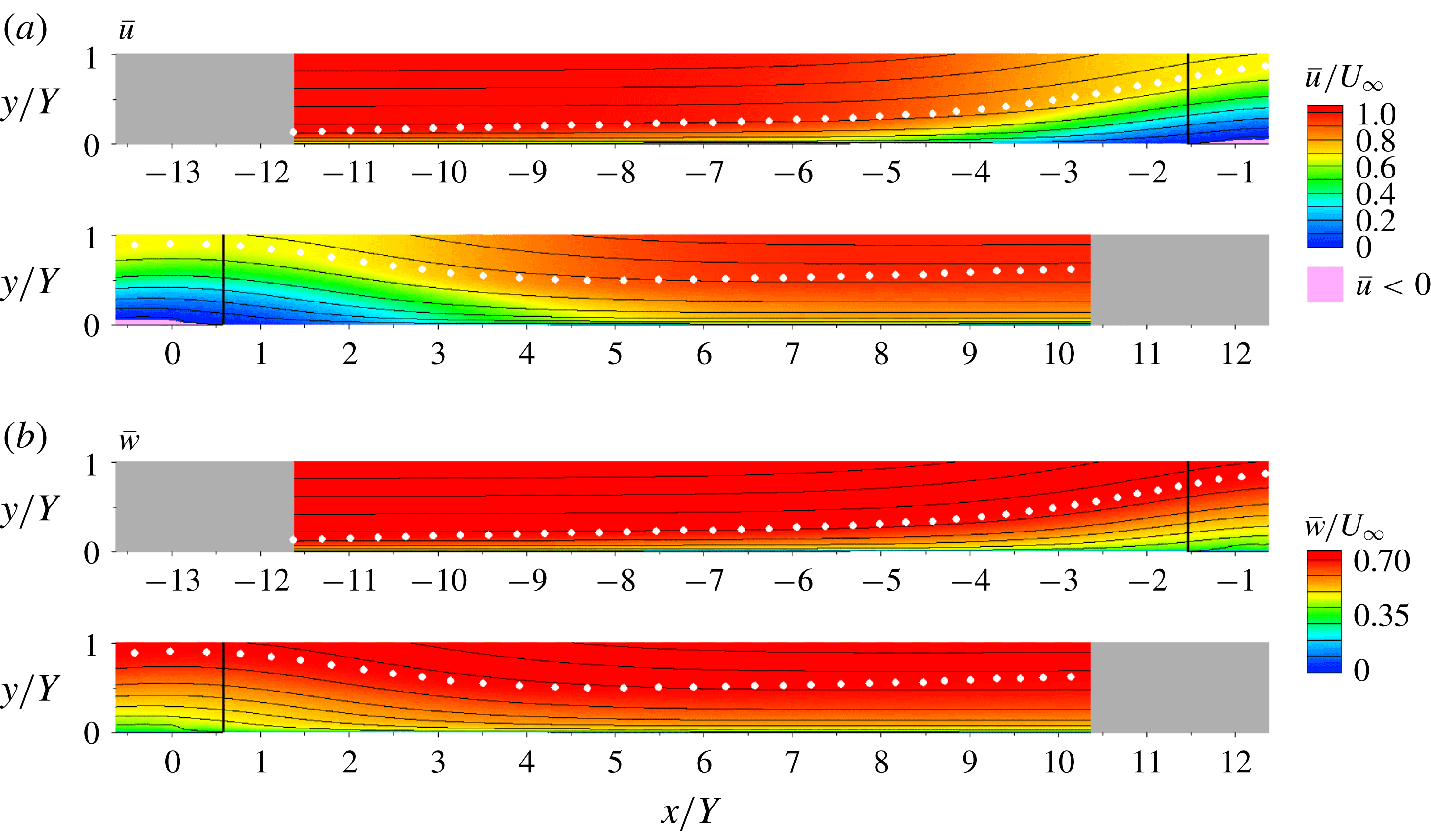
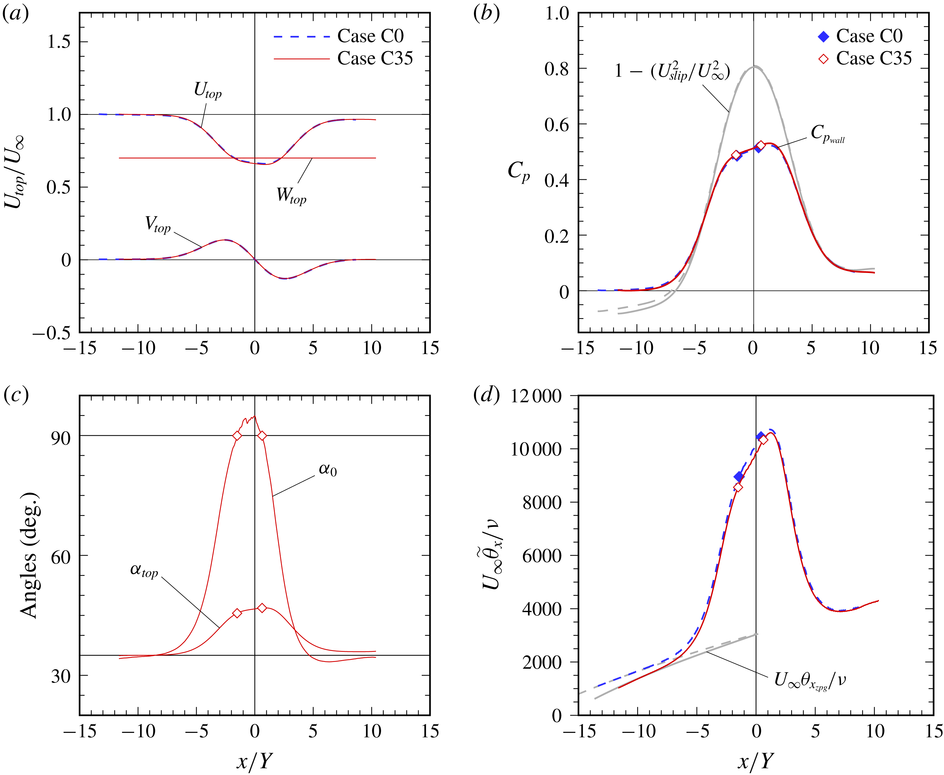
Figure 1 provides an overview of the new flow (Case C35), and figure 2 a comparison with its unswept counterpart (Case C0). Figure 2(d) is particularly important.
2.1 Flow definition, numerical strategy
The equation set and numerical strategy are identical to those used in CRS18. The approach involves pseudospectral DNS of a fully turbulent incompressible ZPG boundary layer over a flat no-slip surface, subjected to first APG then FPG conditions (figure 1). The chordwise (
 $x$
-direction) pressure gradients are induced by a chordwise transpiration profile
 $V_{top}(x)$
through a parallel plane offset a fixed distance
 $Y$
from the no-slip surface. The strength and duration of the pressure gradients are set by the maximum velocity
 $V_{max}$
and length scale
 $\unicode[STIX]{x1D70D}$
of the transpiration profile,
 $$\begin{eqnarray}V_{top}(x)=-\sqrt{2}V_{max}\left[\frac{x}{\unicode[STIX]{x1D70D}}\right]\exp \left(\frac{1}{2}-\left[\frac{x}{\unicode[STIX]{x1D70D}}\right]^{2}\right)+\unicode[STIX]{x1D711}_{top},\end{eqnarray}$$
with
 $x=0$
defined as the location at which
 $V_{top}$
changes from suction to blowing (figure 2
a). The last term in (2.1),
 $\unicode[STIX]{x1D711}_{top}$
, is the magnitude of a (small) constant ‘bleed’ velocity, adjusted to offset the blockage in the nominally ZPG regions, and thereby produce
 $\text{d}P/\text{d}x\approx 0$
along the wall there.
Mean streamlines and contours of (a) chordwise
 $\bar{u}$
and (b) spanwise
 $\bar{w}$
velocity in chordwise–wall-normal plane for Case C35. Shaded/grey regions are fringe zones. Solid vertical lines indicate stations at which mean chordwise wall stress is zero. White symbols denote edge of boundary layer defined by mean spanwise vorticity (CRS18).

Case parameters. Sweep angle
 $\unicode[STIX]{x1D70E}=\arctan (W_{\infty }/U_{\infty })$
. Chordwise component of upstream/reference velocity magnitude is
 $U_{\infty }$
, such that the total/streamwise magnitude is
 $Q_{\infty }=$
 $U_{\infty }/\cos \unicode[STIX]{x1D70E}=(U_{\infty }^{2}+W_{\infty }^{2})^{1/2}$
, where
 $W_{\infty }$
is the spanwise component.

Chordwise variation of (a) velocity components at
 $y=Y$
, (b) mean wall pressure,
 $C_{p_{wall}}=(\bar{p}_{wall}-P_{\infty })/{\textstyle \frac{1}{2}}\unicode[STIX]{x1D70C}U_{\infty }^{2}$
, (c) angles of surface shear
 $\unicode[STIX]{x1D6FC}_{0}=\arctan (\unicode[STIX]{x1D70F}_{w_{z}}/\unicode[STIX]{x1D70F}_{w_{x}})$
and velocity at
 $y=Y$
,
 $\unicode[STIX]{x1D6FC}_{top}=\arctan (W_{top}/U_{top})$
and (d) chordwise momentum-thickness Reynolds number: symbols,
 $\unicode[STIX]{x1D70F}_{w_{x}}=0$
locations; shaded/grey curves, (in b) blockage-free wall pressure variation associated with slip velocity
 $U_{slip}$
induced by
 $V_{top}$
(see CRS18) and (in d) virtual Reynolds-number variation given by ZPG thickness
 $\unicode[STIX]{x1D703}_{x_{zpg}}$
from Coles (Reference Coles1962) (see figure 3
b and its legend). Chordwise momentum thickness
 $\widetilde{\unicode[STIX]{x1D703}}_{x}$
is defined in terms of mean spanwise vorticity (equation (3.4) of CRS18).

We compute a single new case, denoted C35, which is a
 $\unicode[STIX]{x1D70E}=35^{\circ }$
infinite-swept-wing version of Case C of CRS18, in the sense that the transpiration profile – and thus the pressure-gradient variation – of the latter is applied along the chordwise direction of the swept flow, with the same chordwise Reynolds number
 $U_{\infty }Y/\unicode[STIX]{x1D708}$
. We shall henceforth refer to Case C, the highest-Reynolds-number flow presented in CRS18, as ‘Case C0’, as a reminder of its unswept state. As was true for Case C0, the transpiration parameters in table 1 yield an APG/FPG variation that creates a small separation ‘bubble’ (strip), with mean detachment/reattachment lines parallel to the leading edge (see figures 4
b and 6, below). While this bubble differs from some found elsewhere, in that its reattachment is controlled by an imposed FPG, rather than by a spreading shear layer (e.g. Greenblatt et al.
Reference Greenblatt, Paschal, Yao, Harris, Schaeffler and Washburn2006), the process by which it forms, especially in the ZPG/APG regions leading up to separation, is typical of many applications.
Figure 2 compares Cases C0 and C35. They have identical
 $U_{top}$
and
 $V_{top}$
, with finite
 $W_{top}$
distinguishing C35 (figure 2
a). Figure 2(b) shows the wall pressure (including the blockage-free variation). Figure 2(c) illustrates the change along the chordwise axis of the directions of the local wall shear and top-wall velocity for Case C35.
Figure 2(d) presents the chordwise momentum-thickness Reynolds numbers. In order to make the comparison between the swept and unswept flows as meaningful as possible (when, for example, examining the validity of the Independence Principle), Case C35 is defined such that the momentum-thickness Reynolds number of its mean chordwise velocity component in the upstream ZPG region and that of the mean streamwise component in the same region of Case C0, ‘aim at the same target’. This is done by adjusting the
 $x=0$
location of the Case C35 transpiration profile such that the chordwise ZPG layer’s virtual thickness at
 $x=0$
,
 $\unicode[STIX]{x1D703}_{x_{0}}$
(defined as the thickness that would exist were the APG not applied), is close to the
 $\unicode[STIX]{x1D703}_{x_{0}}$
of Case C0. The matching is based on the behaviour observed in the Coles (Reference Coles1962) experiments, using the
 $C_{f}=C_{f}(R_{\unicode[STIX]{x1D703}})$
interpolant shown in figure 3(
 $b$
), and the ZPG von Kármán momentum integral equation (MIE). The result is
 $U_{\infty }\unicode[STIX]{x1D703}_{x_{0}}/\unicode[STIX]{x1D708}\approx 3000$
for both the
 $\unicode[STIX]{x1D70E}=0$
and
 $35^{\circ }$
cases (see table 1 and shaded/grey curves in figure 2
d). At the ZPG reference stations (see § 3.1), the streamwise Reynolds number has changed from
 $U_{\infty }\unicode[STIX]{x1D703}/\unicode[STIX]{x1D708}=1744$
for Case C0 to 1681 for Case C35. The fact that these differ by more than the corresponding values of
 $U_{\infty }\unicode[STIX]{x1D703}_{x_{0}}/\unicode[STIX]{x1D708}$
do (3057 versus 3031), is an indication of the behaviour described in the Introduction, that the IP must fail in the ZPG region of a fully turbulent collateral layer.
Numerical parameters. Origin of chordwise coordinate
 $x$
, and thus locations of inflow
 $x_{in}$
and outflow
 $x_{out}$
stations, is defined by location of sign change of transpiration profile
 $V_{top}(x)$
, with
 $x_{out}-x_{in}=\unicode[STIX]{x1D6EC}_{x}$
, where
 $\unicode[STIX]{x1D6EC}_{x}$
is the streamwise period of the domain (see figure 2
a and main text); spanwise period is
 $\unicode[STIX]{x1D6EC}_{z}$
. Dealiasing is enforced by defining the number of quadrature/collocation points,
 $N_{x}$
,
 $N_{y}$
and
 $N_{z}$
, such that they are related to the number of streamwise, wall-normal and spanwise Galerkin spectral expansion coefficients, respectively, by
 $M_{x}=2N_{x}/3$
,
 $M_{y}=(2N_{y}-9)/3$
and
 $M_{z}=2N_{z}/3$
. Spatial resolution is quantified in terms of the quadrature grid, such that
 $\unicode[STIX]{x0394}x=\unicode[STIX]{x1D6EC}_{x}/N_{x}$
and
 $\unicode[STIX]{x0394}z=\unicode[STIX]{x1D6EC}_{z}/N_{z}$
; the distance
 $y_{10}$
is that of the tenth wall-normal quadrature point from the bottom of the domain (with
 $y_{1}=0$
). Wall units, e.g.
 $\unicode[STIX]{x0394}x^{+}=\unicode[STIX]{x0394}xu_{\unicode[STIX]{x1D70F}}/\unicode[STIX]{x1D708}$
and
 $y_{10}^{+}=y_{10}u_{\unicode[STIX]{x1D70F}}/\unicode[STIX]{x1D708}$
, are based on maximum skin friction within the domain, downstream of the fringe zone.

Readers primarily interested in physical results may wish to skip the next section, and move directly to § 3.
2.2 Further computational details
The numerical parameters are summarized in table 2. The differences for Cases C0 and C35 in the inflow and outflow coordinates,
 $x_{in}$
and
 $x_{out}$
, are the result of altering the
 $x=0$
transpiration location, as described above. The chordwise
 $\unicode[STIX]{x1D6EC}_{x}$
and spanwise
 $\unicode[STIX]{x1D6EC}_{z}$
domain sizes are the same for the two cases; the statements in CRS18 (§ 2.2) regarding the suitability of
 $\unicode[STIX]{x1D6EC}_{x}$
and
 $\unicode[STIX]{x1D6EC}_{z}$
for Case C0 also apply to Case C35. (The spanwise size of the instantaneous turbulence structures in the
 $y/Y=0.2$
plane for a swept version of Case A are comparable to those shown in figure 1(c) of CRS18. The half-domain wall-stress visualizations shown in figure 4(b,c) below also support the adequacy of
 $\unicode[STIX]{x1D6EC}_{z}$
.) The number of wall-normal
 $N_{y}$
and spanwise
 $N_{z}$
quadrature/collocation points used for the two flows is also the same. The chordwise resolution for C35, on the other hand, was increased from
 $N_{x}=7680$
to 15 360. These choices are sufficient to capture the smallest, near-wall structures in the swept, collateral ZPG layer upstream of separation (i.e. where
 $u_{\unicode[STIX]{x1D70F}}$
is the largest, and the near-wall streaks are oriented at
 $35^{\circ }$
to the
 $x$
-axis; compare the left-hand-side subplots in figures 4
a and 4
b). The wall-normal resolution for Case C35 is such that the tenth collocation point
 $y_{10}$
is at most
 $5.7\unicode[STIX]{x1D708}/u_{\unicode[STIX]{x1D70F}}$
; this is fully adequate (cf. Spalart, Coleman & Johnstone Reference Spalart, Coleman and Johnstone2009). The maximum chordwise spacing over the domain is
 $\unicode[STIX]{x0394}x^{+}=7.7$
, which is comparable to the spanwise resolution,
 $\unicode[STIX]{x0394}z^{+}=7.1$
. To provide the identical along- and across-streak resolution used for Case C0 (i.e. 12.3 and 6, respectively) for Case C35 would require
 $\unicode[STIX]{x0394}x^{+}=6.2$
and
 $\unicode[STIX]{x0394}z^{+}=5.5$
. (This can be shown by considering the maximum
 $x$
and
 $z$
wavenumbers in the two domains.) As these are not significantly different from the actual spacings, we conclude the Case C35 resolution is sufficient in the attached regions. That the resolution is also adequate for the near-wall structures near the separation zone is strongly suggested by the subplots in figure 4(b); note that the minimum tick-mark spacing corresponds to approximately six collocation points in the chordwise and spanwise directions. As in CRS18, the most serious challenge to the resolution is provided by the shear layer above the separation bubble, where the ratio of the wall-normal grid spacing
 $\unicode[STIX]{x0394}y$
to the local Kolmogorov length
 $\unicode[STIX]{x1D702}$
is the largest. Even so,
 $\unicode[STIX]{x0394}y/\unicode[STIX]{x1D702}$
does not exceed ten here, and is thus marginally acceptable for spectral discretizations (Moin & Mahesh Reference Moin and Mahesh1998). The chordwise
 $\unicode[STIX]{x0394}x/\unicode[STIX]{x1D702}$
and spanwise
 $\unicode[STIX]{x0394}z/\unicode[STIX]{x1D702}$
ratios are largest (both of order 5) at the wall in the collateral/ZPG region.
The chordwise (inflow/outflow) boundary conditions are applied using the ‘fringe method’ introduced by Spalart & Watmuff (Reference Spalart and Watmuff1993), which involves adding forcing terms to the governing equations that are only active in the regions indicated by the shaded/grey zones in figure 1. This allows the chordwise-periodic spectral method to accommodate the
 $x$
-wise variation of the mean flow. The fringe parameters used here are identical to those specified in appendix A of CRS18 (i.e.
 $x_{1}/Y=1.0$
,
 $V_{2}/U_{\infty }=1.5$
,
 $\unicode[STIX]{x1D6F6}=2.0$
,
 $y_{\unicode[STIX]{x1D6FD}}/Y=0.16$
), except for
 $y_{\unicode[STIX]{x1D6FC}}/Y$
, which was decreased from 0.518 to 0.455. The spectral algorithm imposes periodic boundary conditions in the spanwise infinite sweep direction
 $z$
. The Galerkin basis functions are Jacobi polynomials in
 $\unicode[STIX]{x1D701}\in [0,1]$
, mapped to the
 $y\in [0,\infty ]$
domain via
 $\unicode[STIX]{x1D701}=\exp (-y/y_{0})$
, where
 $y_{0}$
is the mapping length scale (Spalart, Moser & Rogers Reference Spalart, Moser and Rogers1991); for both Cases C0 and C35,
 $y_{0}=0.343Y$
.
The new boundary condition on the spanwise velocity is enforced by adding
 $(1-\exp (-y/y_{0}))W_{\infty }$
to the spanwise component of the computational variable
 $\boldsymbol{U}_{1}$
(see Spalart et al. (Reference Spalart, Moser and Rogers1991) and Spalart & Coleman (Reference Spalart and Coleman1997)), where
 $W_{\infty }$
is the constant spanwise velocity above the layer. The mean vorticity and mean viscous terms are altered as in Coleman, Ferziger & Spalart (Reference Coleman, Ferziger and Spalart1990). The corresponding change to the finite-domain version of the top-wall boundary condition (equivalent to the
 $y\rightarrow \infty$
form used here) is the replacement of
 $\unicode[STIX]{x2202}w/\unicode[STIX]{x2202}y=0$
with
 $w=W_{\infty }$
in (2.2c) of CRS18. The ability of the code to represent collateral conditions in the ZPG zones (§ 3.1), and to capture the mean hodograph evolution (figure 10), imply the modifications involving the spanwise velocity were implemented correctly.
Statistics were gathered by averaging over
 $z$
and time, involving 78 full
 $x$
–
 $y$
fields over periods of 33.5 and
 $54Y/U_{\infty }$
, respectively, for Cases C0 and C35, corresponding to 1.3 and 2.1 domain-flow-through times
 $\unicode[STIX]{x1D6EC}_{x}/U_{\infty }$
. (The results in figure 5 are from a subset of the full sample.) Some quantities were also locally averaged in
 $x$
, with a filter width as large as
 $0.1Y$
. The momentum balances associated with the resulting statistics are very good, comparable, in both the
 $x$
and
 $z$
directions, to the
 $x$
balance shown in appendix C of CRS18; see also inset plot in figure 7(b). The
 $z$
- and
 $t$
-averaged data are available from the turbulence modelling resource (TMR) website, https://turbmodels.larc.nasa.gov.
Computations were run on the NASA Advanced Supercomputing (NAS) Division’s Pleiades system, a distributed-memory SGI ICE cluster, on from 1024 to 4096 cores. A total of approximately 512 000 CPU-core hours were utilized during the statistics-gathering phase of the Case C35 computations.
3 Results
3.1 ZPG reference state and the IP
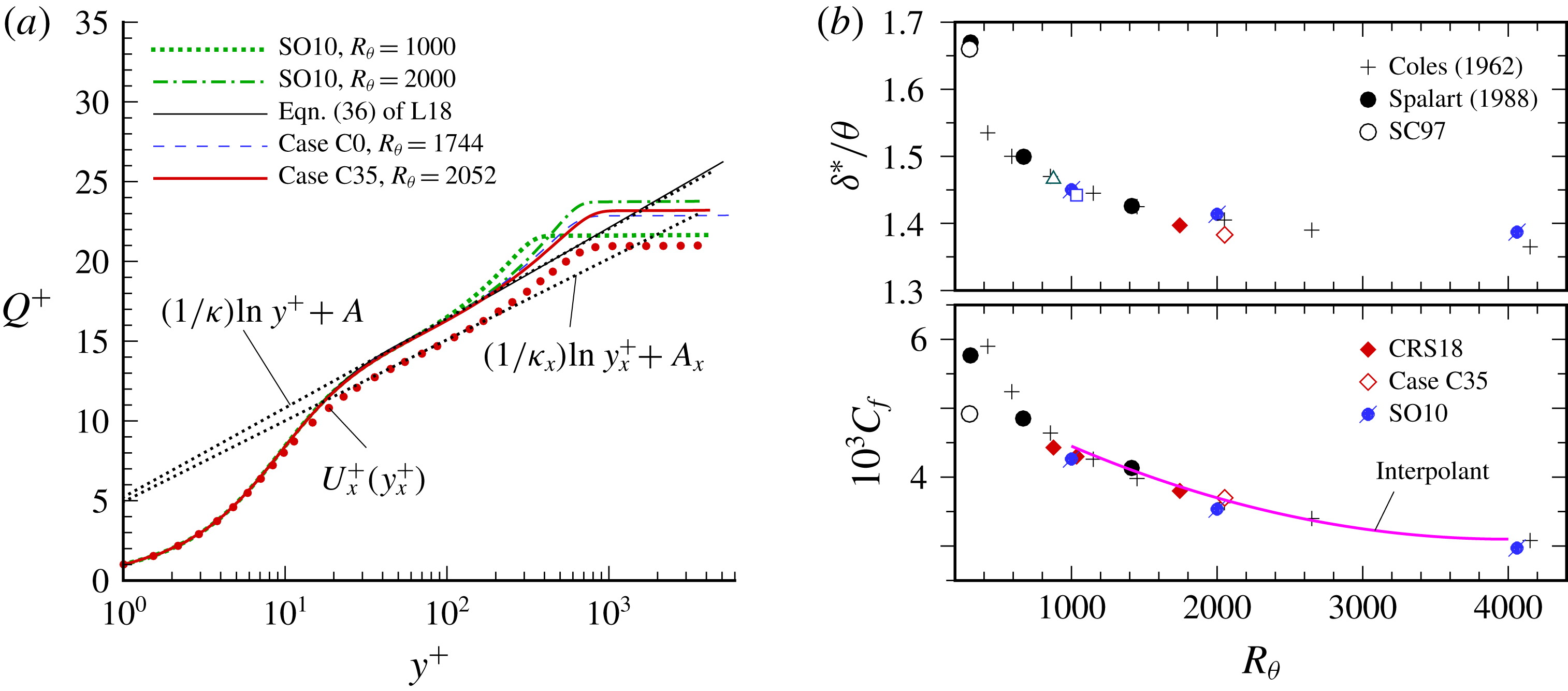
(a) Mean-velocity profiles at ZPG reference stations, and ZPG turbulent boundary layer DNS of Schlatter & Örlü (Reference Schlatter and Örlü2010) (SO10): ● (red),
 $U_{x}^{+}$
versus
 $y_{x}^{+}$
for Case C35, where
 $U_{x}^{+}=\bar{u}/u_{\unicode[STIX]{x1D70F}_{x}}$
,
 $y_{x}^{+}=yu_{\unicode[STIX]{x1D70F}_{x}}/\unicode[STIX]{x1D708}$
and
 $u_{\unicode[STIX]{x1D70F}_{x}}^{2}=\unicode[STIX]{x1D708}(\unicode[STIX]{x2202}\bar{u}/\unicode[STIX]{x2202}y)_{w}$
;
 $\cdots \cdots$
, logarithmic profiles in terms of standard von Kármán and additive constants,
 $\unicode[STIX]{x1D705}$
and
 $A$
, and
 $\unicode[STIX]{x1D705}_{x}$
and
 $A_{x}$
for the chordwise component of a collateral layer, with
 $\unicode[STIX]{x1D705}_{x}=\unicode[STIX]{x1D705}/\sqrt{\cos \unicode[STIX]{x1D70E}}$
,
 $A_{x}=A\sqrt{\cos \unicode[STIX]{x1D70E}}-\ln (\cos \unicode[STIX]{x1D70E})/2\unicode[STIX]{x1D705}_{x}$
, using
 $\unicode[STIX]{x1D705}=0.41$
,
 $A=5.2$
; —— (grey), equation (36) of Luchini (Reference Luchini2018) (L18). (b) Shape factor and skin friction: —— (magenta), interpolant of Coles data:
 $C_{f}=a+bR_{\unicode[STIX]{x1D703}}+cR_{\unicode[STIX]{x1D703}}^{2}$
, with
 $(a,b,c)=(0.0055,-1.2\times 10^{-6},1.5\times 10^{-10})$
, where
 $C_{f}=\unicode[STIX]{x1D70F}_{w}/{\textstyle \frac{1}{2}}\unicode[STIX]{x1D70C}Q_{\infty }^{2}$
.

A high priority was to specify standard ZPG conditions upstream of the APG. This is an essential feature for DNS (or experimental) data that are to be used to isolate PG effects and to serve as a benchmark for RANS-model testing, or that of other turbulence-resolving approaches for that matter. That this objective was met can be inferred from figure 3. The ZPG reference station was chosen as
 $x/Y=-9.5$
and
 $-8.5$
respectively for Cases C0 and C35. Recall that for Case C35 the (collateral) 2-D ZPG layer is directed at
 $35^{\circ }$
away from the
 $x$
-axis (see the solid black lines in figure 10). The mean-velocity profiles, the displacement/momentum-thickness shape factor, and the skin friction are all characteristic of constant free-stream velocity boundary layers at their respective Reynolds numbers (
 $R_{\unicode[STIX]{x1D703}}=Q_{\infty }\unicode[STIX]{x1D703}/\unicode[STIX]{x1D708}=1744$
for C0, 2052 for C35; the corresponding friction velocities are
 $u_{\unicode[STIX]{x1D70F}}/U_{\infty }=u_{\unicode[STIX]{x1D70F}}/Q_{\infty }=0.0436$
for C0, and
 $u_{\unicode[STIX]{x1D70F}}/U_{\infty }=0.0525$
,
 $u_{\unicode[STIX]{x1D70F}}/Q_{\infty }=0.0430$
for C35). The logarithmic-law scaling of the mean velocity in figure 3(a) is in good agreement with independent DNS datasets and Luchini’s high-Reynolds-number asymptote. In addition, the skewness statistics of the instantaneous surface stress of the ZPG states of Cases C0 and C35 are also close to each other (see the dotted and chain-dotted probability density functions in figure 5
b). The
 $R_{\unicode[STIX]{x1D703}}$
dependence of
 $\unicode[STIX]{x1D6FF}^{\ast }/\unicode[STIX]{x1D703}$
and
 $C_{f}$
(lower figure 3
b) for both cases is consistent with previous DNS (Spalart Reference Spalart1988; Schlatter & Örlü Reference Schlatter and Örlü2010), and the Coles (Reference Coles1962) data for ZPG boundary layers. The Case C35 turbulence kinetic energy (TKE) profile and individual budget terms (not shown), also agree well with Schlatter & Örlü’s (Reference Schlatter and Örlü2010) ZPG DNS at
 $R_{\unicode[STIX]{x1D703}}=2000$
(as it did for Case C0; see figure 6 of CRS18), although the correspondence for the Case C35 outer-layer TKE profile is not quite as good as it is for Case C0. This agreement, for various quantities, underlines the success of the fringe-zone inflow/outflow treatment, in allowing a spatially developing flow to be faithfully represented in a periodic domain, and the sufficient length of development toward a universal ZPG state defined solely by
 $R_{\unicode[STIX]{x1D703}}$
.
The solid line in figure 3(b) is a curve fit of the
 $C_{f}$
versus
 $R_{\unicode[STIX]{x1D703}}$
relationship found in the Coles results. As mentioned above, this was used to estimate the chordwise variation of the chordwise momentum thickness of the virtual (chordwise) ZPG boundary layer into the APG region – and thus set the origin (i.e. location of the APG-to-FPG transition) for the transpiration profile
 $V_{top}(x)$
. Consequently, the chordwise momentum thickness at
 $x=0$
,
 $\unicode[STIX]{x1D703}_{x_{0}}$
, for Case C35 is close to
 $\unicode[STIX]{x1D703}_{x_{0}}(=\unicode[STIX]{x1D703}_{_{0}})$
for Case C0; see figure 2(a,d).
We conclude this section by pointing to the red symbols in figure 3(a), which illustrate the chordwise component of the Case C35 mean velocity, scaled in terms of the chordwise component of the surface shear stress,
 $U_{x}^{+}=\bar{u}/u_{\unicode[STIX]{x1D70F}_{x}}$
versus
 $y_{x}^{+}=yu_{\unicode[STIX]{x1D70F}_{x}}/\unicode[STIX]{x1D708}$
. The deviation of
 $U_{x}^{+}\!(y_{x}^{+})$
from the standard logarithmic profile exhibited by the full 2-D profile magnitude (solid red curve; cf. upper dotted reference line), and its good agreement with the logarithmic reference that uses the modified, sweep-dependent, chordwise constants
 $\unicode[STIX]{x1D705}_{x}$
and
 $A_{x}$
(lower dotted reference line), confirms the breakdown of the IP for the fully turbulent ZPG layer, as described in the Introduction. The question of the IP’s validity in the APG and FPG regions will be addressed below.
3.2 Chordwise development of the flow
3.2.1 Skin friction
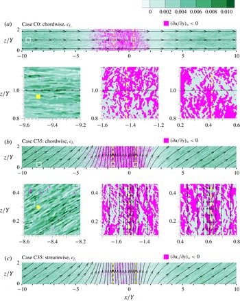
Visualizations of instantaneous (a,b) chordwise
 $c_{f_{x}}$
and (c) streamwise
 $c_{f_{s}}$
components of wall shear stress for (a) Case C0 and (b,c) Case C35, where
 $c_{f_{x}}=\unicode[STIX]{x1D708}(\unicode[STIX]{x2202}u/\unicode[STIX]{x2202}y)_{w}/{\textstyle \frac{1}{2}}U_{\infty }^{2}$
and
 $c_{f_{s}}=\unicode[STIX]{x1D708}(\unicode[STIX]{x2202}u_{s}/\unicode[STIX]{x2202}y)_{w}/{\textstyle \frac{1}{2}}Q_{\infty }^{2}$
, with
 $u_{s}=u\cos \unicode[STIX]{x1D70E}+w\sin \unicode[STIX]{x1D70E}$
and
 $\tan \unicode[STIX]{x1D70E}=W_{\infty }/U_{\infty }=0.7$
. Dashed lines,
 $\unicode[STIX]{x1D70F}_{w_{x}}=0$
locations; solid curves/arrows, mean limiting surface streamlines. The three subplots in each of (a) and (b) are from subregions indicated by white squares in plot above; tick-mark spacing in subplots corresponds to
 $2.95\unicode[STIX]{x0394}x$
and
 $6.4\unicode[STIX]{x0394}z$
for (a) Case C0 and
 $5.9\unicode[STIX]{x0394}x$
and
 $6.4\unicode[STIX]{x0394}z$
for (b) Case C35. Filled yellow symbol in left-hand side subplots is 100 local wall units square. The
 $-10\leqslant x/Y\leqslant 10$
,
 $0\leqslant z/Y\leqslant 2$
subdomain shown is 77 % and 50 % respectively of the full
 $(\unicode[STIX]{x1D6EC}_{x},\unicode[STIX]{x1D6EC}_{z})=(26Y,4Y)$
domain.

Visualizations of the instantaneous surface stress are presented in figure 4, for Cases C0 and C35. The magenta contours indicate regions of local flow reversal, with respect to either the chordwise (
 $x$
) direction (in a and b) or the one aligned with
 $\boldsymbol{Q}_{\infty }=U_{\infty }\hat{\boldsymbol{e}}_{x}+W_{\infty }\hat{\boldsymbol{e}}_{z}$
(in c). The dashed lines mark the locations of zero mean total (Case C0) or chordwise (C35) surface stress. The solid curves/arrows in figure 4(b,c), which trace the mean surface streamlines defined by the total stress, reveal the characteristic swept-wing pattern of surface streamline convergence into the separation line (White Reference White1991; McLean Reference McLean2013), and divergence out of the reattachment line. The instantaneous chordwise-reversal contours for the swept and unswept cases are similar in terms of their chordwise size, leading to mean separation bubbles of nearly the same location and extent (see subplots in figure 4
a,b); the
 $c_{f_{x}}\leqslant 0$
contours are longer in the spanwise direction for Case C35, as befits a flow whose near-wall structures are affected by non-zero spanwise shear
 $\unicode[STIX]{x2202}\bar{w}/\unicode[STIX]{x2202}y$
at the wall. Elsewhere, the elongated/streaky structures beneath the ZPG regions up- and downstream of their respective separation zones have, despite their different orientations, similar spacings and aspect ratios, consistent with the agreement of the total mean-velocity profiles at the ZPG reference stations (figure 3
a). (The solid yellow square in the left-hand subplots in figure 4(a,b) correspond to 100 local wall units.)
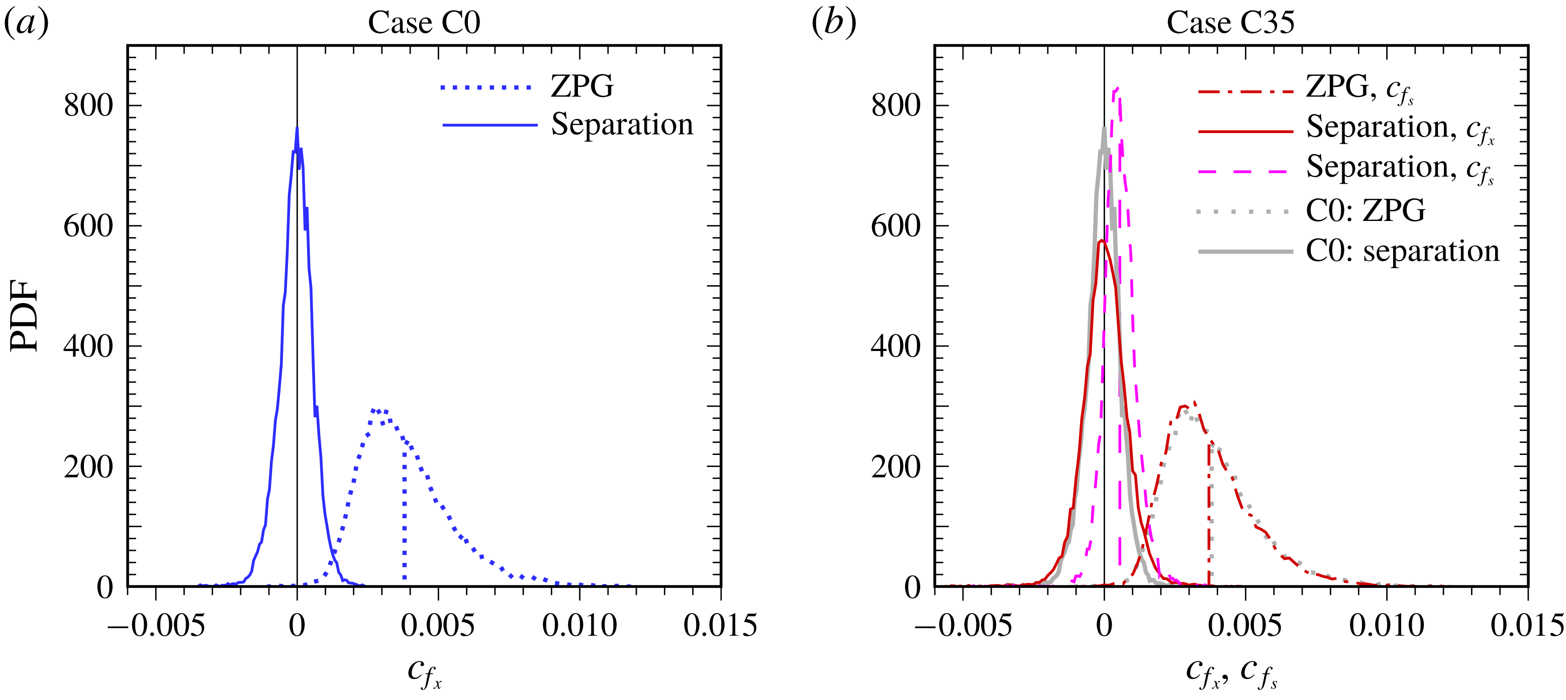
Probability density function
 $\text{PDF}$
of instantaneous chordwise
 $c_{f_{x}}$
and streamwise
 $c_{f_{s}}$
surface shear stress. (a) Case C0:
 $\cdots \cdots$
,
 $x/Y=-9.5$
(ZPG reference station); —— (blue),
 $x/Y=-1.43$
(mean separation location). (b) Case C35: — ⋅ — (red),
 $c_{f_{s}}$
at
 $x/Y=-8.5$
(ZPG reference); —— (red),
 $c_{f_{x}}$
at
 $x/Y=-1.51$
(
 $\unicode[STIX]{x1D70F}_{w_{x}}=0$
); - - - - (red),
 $c_{f_{s}}$
at
 $x/Y=-1.51$
; shaded/grey curves in (b) are Case C0 results from (a). Vertical lines indicate mean values.

The probability density functions (PDFs) of the instantaneous surface stress corresponding to figure 4 are shown in figure 5. The PDFs from the ZPG regions are nearly coincident for Cases C0 and C35, which emphasizes the standard ZPG behaviour upstream of the APG in both flows; note the close agreement between the dotted and chain-dotted curves in figure 5(b) (the chordwise
 $c_{f_{x}}$
and streamwise
 $c_{f_{s}}$
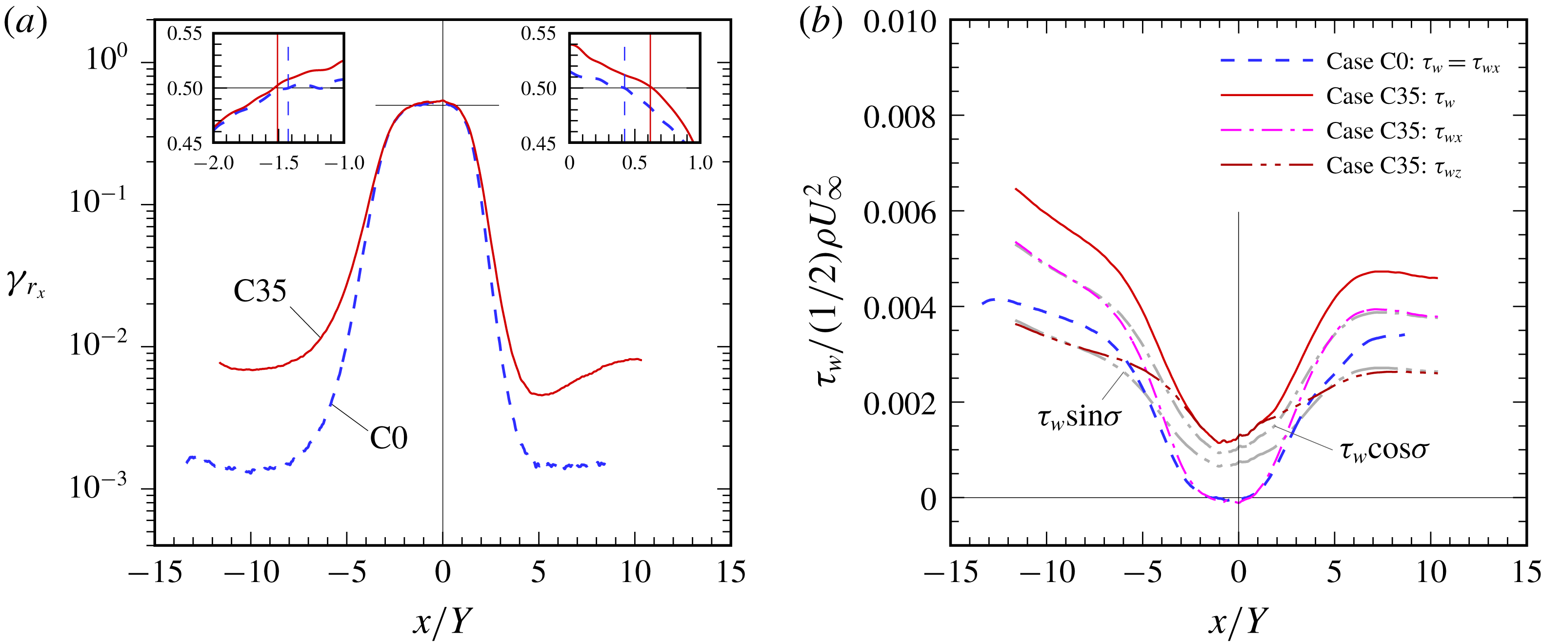
components are compared to account for the swept/collateral condition of Case C35). Both PDFs are skewed towards larger-magnitude positive events, as is typical of attached wall layers (Kim, Moin & Moser Reference Kim, Moin and Moser1987). Nearer the separation bubble, the chordwise-component PDFs for both flows becomes more Gaussian, such that at mean separation the skewness is essentially zero, with Case C35 having a slightly wider distribution. (The somewhat non-Gaussian character for Case C35 of the streamwise component at separation (red-dashed curve) reflects the non-zero spanwise surface stress.) This is consistent with the close agreement between the locations of the 50 % chordwise reversal (
 $\unicode[STIX]{x1D6FE}_{r_{x}}=0.5$
) stations and those of the zero mean chordwise stress (
 $C_{f_{x}}=0$
), at both separation and reattachment, for both
 $\unicode[STIX]{x1D70E}=0$
and
 $35^{\circ }$
(figure 6
a inset plots). The rare but non-zero incidents of flow reversal well upstream of the APG indicated in figure 6(a) are typical of all but the lowest Reynolds numbers (and not, in the ZPG regions, an indication of impending separation); these become increasingly common with increasing
 $Re$
(Spalart Reference Spalart1988; cf. figure 7b of CRS18). The higher
 $\unicode[STIX]{x1D6FE}_{r_{x}}$
values for Case C35 in the ZPG region are a consequence of only examining the
 $x$
-wise component of the instantaneous wall shear (contrast figures 4
b and 4
c).
Chordwise variation of (a) fraction of reversed chordwise wall shear
 $\unicode[STIX]{x1D6FE}_{r_{x}}$
and (b) skin friction. Horizontal lines in (a) denote
 $\unicode[STIX]{x1D6FE}_{r_{x}}=0.50$
threshold; vertical lines in inset plots indicate
 $\unicode[STIX]{x1D70F}_{w_{x}}=0$
locations. Shaded/grey curves in (b),
 $\unicode[STIX]{x1D70F}_{w}\cos \unicode[STIX]{x1D70E}$
and
 $\unicode[STIX]{x1D70F}_{w}\sin \unicode[STIX]{x1D70E}$
for Case C35.

An unambiguous answer to the question regarding the validity of the IP for turbulent separated boundary layers over swept wings can be inferred from figure 6(b). The complete success of the IP would be expressed by agreement of the total
 $C_{f}=\unicode[STIX]{x1D70F}_{w}/{\textstyle \frac{1}{2}}\unicode[STIX]{x1D70C}U_{\infty }^{2}$
variation for Case C0 (dashed blue curve) with that of the chordwise component
 $\unicode[STIX]{x1D70F}_{w_{x}}/{\textstyle \frac{1}{2}}\unicode[STIX]{x1D70C}U_{\infty }^{2}$
for Case C35 (chain-single-dotted magenta). The shaded/grey curves trace the variation of the chordwise and spanwise components of the total Case C35 stress. The regions where these respectively agree with
 $\unicode[STIX]{x1D70F}_{w_{x}}$
and
 $\unicode[STIX]{x1D70F}_{w_{z}}$
correspond to the collateral zones (cf. figure 10
c,d).
As asserted in the Introduction, and demonstrated in figures 2(d) and especially 3(a), the IP does not hold in the reoriented-2-D (collateral) ZPG zones upstream and downstream of the separation bubble. However, as the pressure gradient becomes stronger, and the relative importance of the turbulence stress fades (see § 3.2.3), the IP becomes increasingly valid: the projection of the total flow onto the chordwise–wall-normal plane approaches the unswept flow, and the corresponding skin-friction trajectories converge, to the point that the locations of mean separation and reattachment for the two flows are quite close:
 $x/Y=-1.43$
and 0.42 for Case C0,
 $x/Y=-1.51$
and 0.62 for Case C35. (The bubble is taller for the swept flow, with the maximum mean height of the dividing streamline equal to
 $0.095Y$
, compared to 0.053 for Case C0.) Based on figure 6(b), we conclude
 $-3\leqslant x/Y\leqslant 3$
is approximately the zone for which the IP is valid. This success has much to do with the decision to give the two flows the same thickness precisely at the location of the separation bubble, and the same pressure gradient; this provided the IP the best chance to succeed, possibly because the flow is stimulated so strongly that inviscid vorticity transport dominates its response (figure 9
b,c).
Regarding the question of the difficulty of RANS predictions of swept separation, relative to the unswept variety, figure 6(b) provides a mixed message. One feature not captured by any of the RANS models applied to Case C0 in CRS18 is not present for Case C35 – namely the delayed recovery downstream of reattachment, where for the unswept case
 $C_{f}$
grows roughly linearly between
 $x/Y\approx 3$
and 6. For the swept layer, this region (which bridges the passage from FPG to collateral conditions) is characterized by more-rapid growth of the chordwise skin friction, yielding behaviour qualitatively similar to that given by the RANS models applied to the unswept flow (see figure 15 of CRS18). The mean three-dimensionality is thus responsible for making this part of the flow more tractable for RANS approaches. Nevertheless, the core difficulty for RANS models resides in the mounting adverse pressure gradient, after leaving the ZPG region (which the models were tuned for), and before the pressure gradients become overwhelming. This difficulty remains regardless of the absence or presence of sweep. The importance of the pressure gradient is addressed in § 3.2.3, after we consider the effect of sweep upon the thickness variations of the swept and unswept layers.
3.2.2 Thicknesses
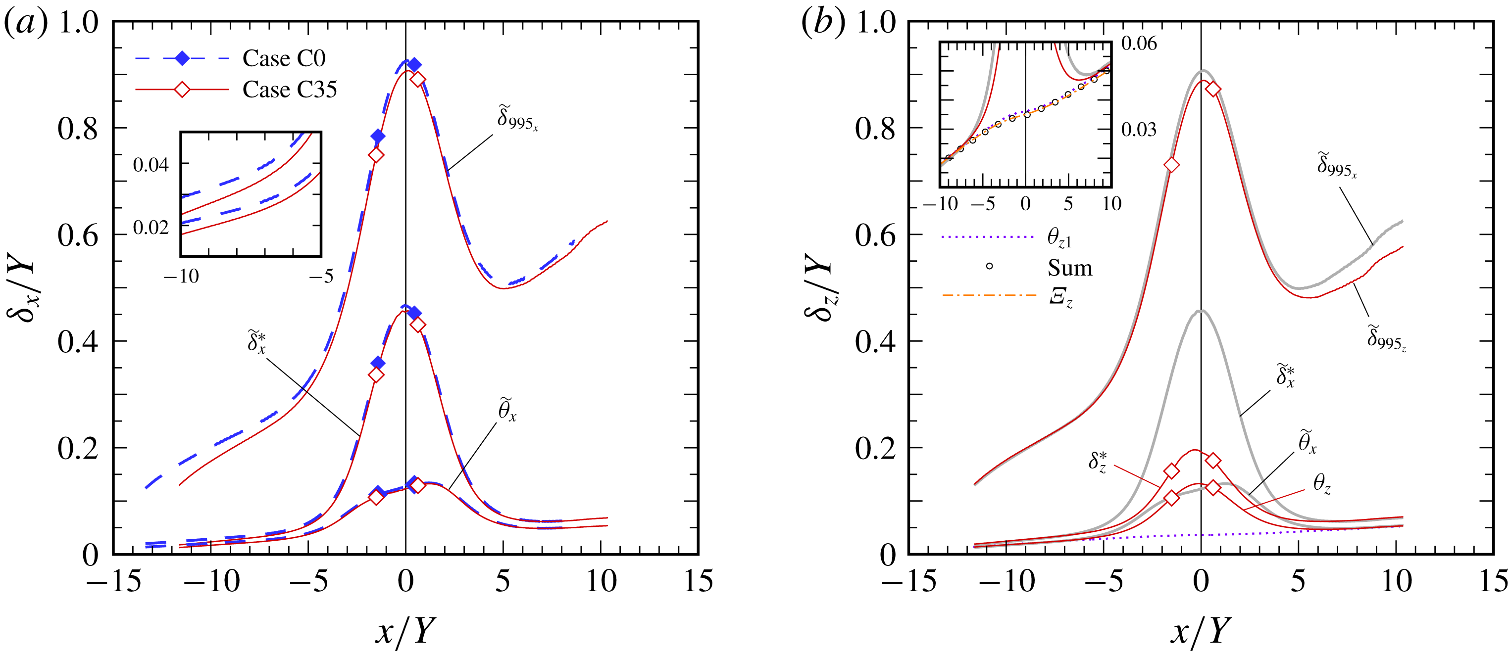
Chordwise variation of (a) chordwise thicknesses for Cases C0 and C35, and (b) spanwise thicknesses for Case C35: diamond symbols,
 $\unicode[STIX]{x1D70F}_{w_{x}}=0$
locations; —— (shaded/grey, in b), chordwise thicknesses for Case C35. Inset plot in (a) shows expanded view of
 $\widetilde{\unicode[STIX]{x1D6FF}_{x}}^{\ast }$
and
 $\widetilde{\unicode[STIX]{x1D703}}_{x}$
upstream of separation. Inset plot in (b) shows terms in integrated spanwise momentum balance for Case C35:
 $\unicode[STIX]{x1D703}_{z1}=\int _{0}^{Y}\bar{u}(W_{\infty }-\bar{w})\,\text{d}y/U_{\infty }W_{\infty }$
,
 $\unicode[STIX]{x1D6EF}_{z}=\int _{x}\unicode[STIX]{x1D70F}_{w_{z}}\,\text{d}x/\unicode[STIX]{x1D70C}U_{\infty }W_{\infty }$
, and sum
 $\unicode[STIX]{x1D703}_{z1}+\unicode[STIX]{x1D703}_{z2}$
, where
 $\unicode[STIX]{x1D703}_{z2}=-\int _{0}^{Y}\overline{u^{\prime }w^{\prime }}\,\text{d}y/U_{\infty }W_{\infty }$
. The chordwise thicknesses
 $\widetilde{\unicode[STIX]{x1D6FF}}_{995_{x}}$
,
 $\widetilde{\unicode[STIX]{x1D6FF}_{x}}^{\ast }$
and
 $\widetilde{\unicode[STIX]{x1D703}}_{x}$
are spanwise-vorticity-based measures defined by equations (3.2)–(3.4) of CRS18; the spanwise thicknesses
 $\unicode[STIX]{x1D6FF}_{995_{z}}$
,
 $\unicode[STIX]{x1D6FF}_{z}^{\ast }$
and
 $\unicode[STIX]{x1D703}_{z}$
are given by standard definitions based on mean spanwise velocity
 $\bar{w}(x,y)$
.

In § 2, we pointed to the difference between the momentum-thickness development in the ZPG regions of the swept and unswept flows (cf. figure 2
d), and stressed how those differences imply failure of the IP there. Recall that Case C35 was designed so that its and Case C0’s chordwise momentum thickness agree at
 $x=0$
, such that deviations of
 $\widetilde{\unicode[STIX]{x1D703}}_{x}$
between the two flows signal a breakdown of the IP. This breakdown is reinforced by figure 7(a), which, in addition to the chordwise momentum thickness
 $\widetilde{\unicode[STIX]{x1D703}}_{x}$
, shows the boundary-layer thickness based on mean spanwise vorticity
 $\widetilde{\unicode[STIX]{x1D6FF}}_{995_{x}}$
and the chordwise displacement thickness
 $\widetilde{\unicode[STIX]{x1D6FF}}_{x}^{\ast }$
. (These generalized, spanwise-vorticity-based measures, denoted by an over-tilde, are used to avoid ambiguities introduced by the non-zero wall-normal gradients of mean velocity in the free stream of non-ZPG boundary layers; see Spalart & Watmuff (Reference Spalart and Watmuff1993) and CRS18.) Under ZPG conditions the Case C0 quantities are consistently larger than those for Case C35. (This is as predicted by the ZPG MIE,
 $\text{d}\unicode[STIX]{x1D703}_{x}/\text{d}x\sim C_{f_{x}}$
, since larger and smaller
 $\unicode[STIX]{x1D703}_{x}$
respectively correspond to smaller and larger
 $\text{d}\unicode[STIX]{x1D703}/\text{d}x$
; cf. figure 6
b.) The success of the IP implied by the skin friction in the region bracketing the separation bubble is manifest here by the coalescence of the Case C0 and C35 variations of (all three versions of) the chordwise thicknesses. (The symbols in figure 7
a indicate the beginning and end of the bubble.)
The standard, velocity-based thicknesses for the spanwise component are presented in figure 7(b) for Case C35; vorticity-based thicknesses would be the same. The shaded curves in this figure are the chordwise counterparts, included for reference. Note the agreement in the ZPG/collateral regions upstream of the bubble between the chordwise and spanwise measures – each of
 $\widetilde{\unicode[STIX]{x1D6FF}}_{995_{x}}$
and
 $\unicode[STIX]{x1D6FF}_{995_{z}}$
,
 $\widetilde{\unicode[STIX]{x1D6FF}}_{995_{x}}^{\ast }$
and
 $\unicode[STIX]{x1D6FF}_{995_{z}}^{\ast }$
, and
 $\widetilde{\unicode[STIX]{x1D703}}_{x}$
and
 $\unicode[STIX]{x1D703}_{z}$
. This is because the APG has yet to cause the direction of the mean velocity to vary with
 $y$
, and the generalized, vorticity-based definitions reduce to the standard, velocity-based ones (since the spanwise component
 $\bar{w}(y)$
is a constant fraction of the total
 $\bar{u}_{s}(y)$
over the entire boundary-layer depth). The rate of growth of
 $\unicode[STIX]{x1D6FF}_{z}^{\ast }$
and
 $\unicode[STIX]{x1D703}_{z}$
(both of which are defined by the velocity component aligned with the direction of no pressure gradient) is significantly larger than that associated with a ZPG layer. It is an indication of the three-dimensionality introduced by the chordwise APG. It is also a consequence of the spanwise component depending upon the chordwise velocity field (which is also true for laminar infinite-swept-wing boundary layers) and, at least indirectly, the turbulent stresses. The evolution of the mean-velocity profiles, and the coupling between chordwise and spanwise components, is considered in § 3.2.4.
The state of the spanwise momentum balance is indicated by the good agreement of the sum of the two non-zero terms and the integrated spanwise skin friction shown in the figure 7(b) inset plot (see legend for definitions). The Reynolds-stress term
 $\unicode[STIX]{x1D703}_{z2}$
is negligible except within the non-zero PG regions. But even there it makes only a slight contribution. The station at which
 $\widetilde{\unicode[STIX]{x1D703}}_{x}$
,
 $\unicode[STIX]{x1D703}_{z}$
, and the primary momentum-balance thickness
 $\unicode[STIX]{x1D703}_{z1}$
diverge is the location downstream of which the APG significantly affects the swept flow. This location,
 $x/Y\approx -6$
, is close to that beyond which the displacement-thickness term in the
 $x$
-wise balance is significant for Case C0 (see figure 17
 $a$
of CRS18).
3.2.3 Reynolds stress
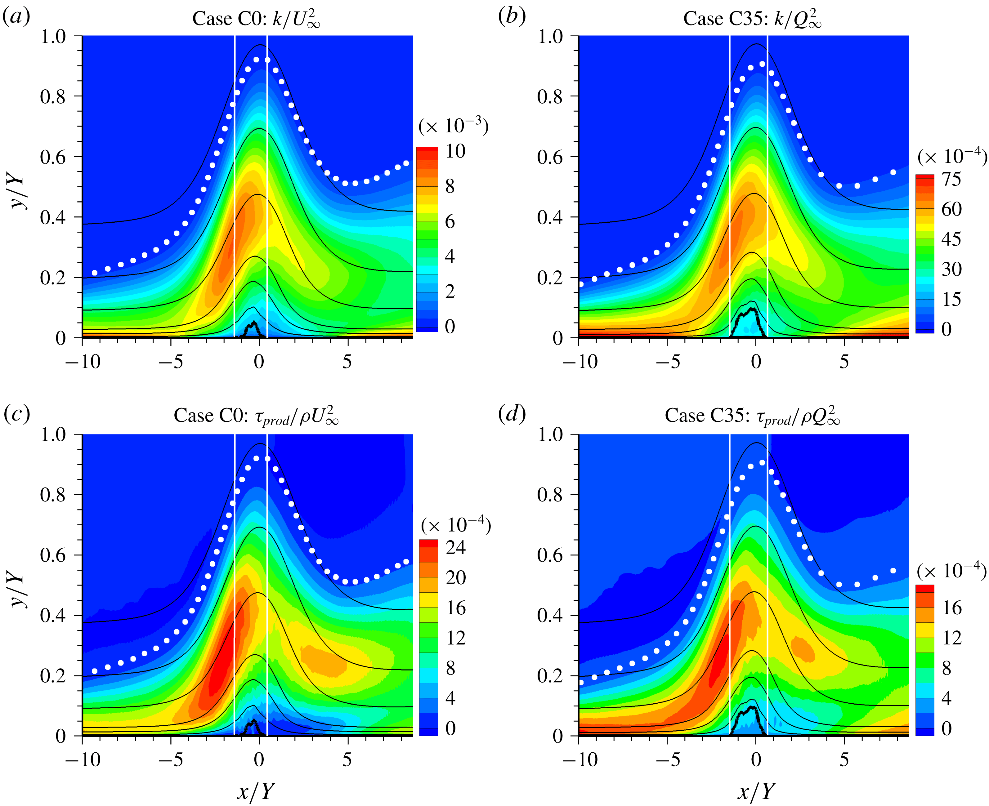
Contours of (a,b) TKE
 $\mathit{k}$
and (c,d) productive shear stress
 $\unicode[STIX]{x1D70F}_{prod}$
for (a,c) Case C0 and (b,d) Case C35. Black curves are mean streamlines; thicker solid curve is the mean dividing streamline of the separation bubble. Solid white vertical lines indicate mean separation and reattachment stations. White symbols denote 99.5 %-boundary-layer thickness
 $\widetilde{\unicode[STIX]{x1D6FF}}_{995}$
.

The TKE fields from Cases C0 and C35 are shown in figure 8. Also shown is the ‘productive stress’ defined by the rates of TKE production and mean strain,
 $\unicode[STIX]{x1D70F}_{prod}=\unicode[STIX]{x1D70C}{\mathcal{P}}_{k}/\sqrt{2S_{ij}S_{ij}}$
(CRS18). (Note the expanded vertical scale, and the different
 $\mathit{k}$
and
 $\unicode[STIX]{x1D70F}_{prod}$
normalizations used for the two cases.) The qualitative agreement for both quantities is striking, especially above the separation zone. Both flows possess a local outer-layer maximum either at (for
 $\mathit{k}$
) or just upstream of (for
 $\unicode[STIX]{x1D70F}_{prod}$
) the separation station. The differences that do exist (in values of the local maxima, and in magnitudes within the bubble) are explored in Coleman, Rumsey & Spalart (Reference Coleman, Rumsey and Spalart2019).
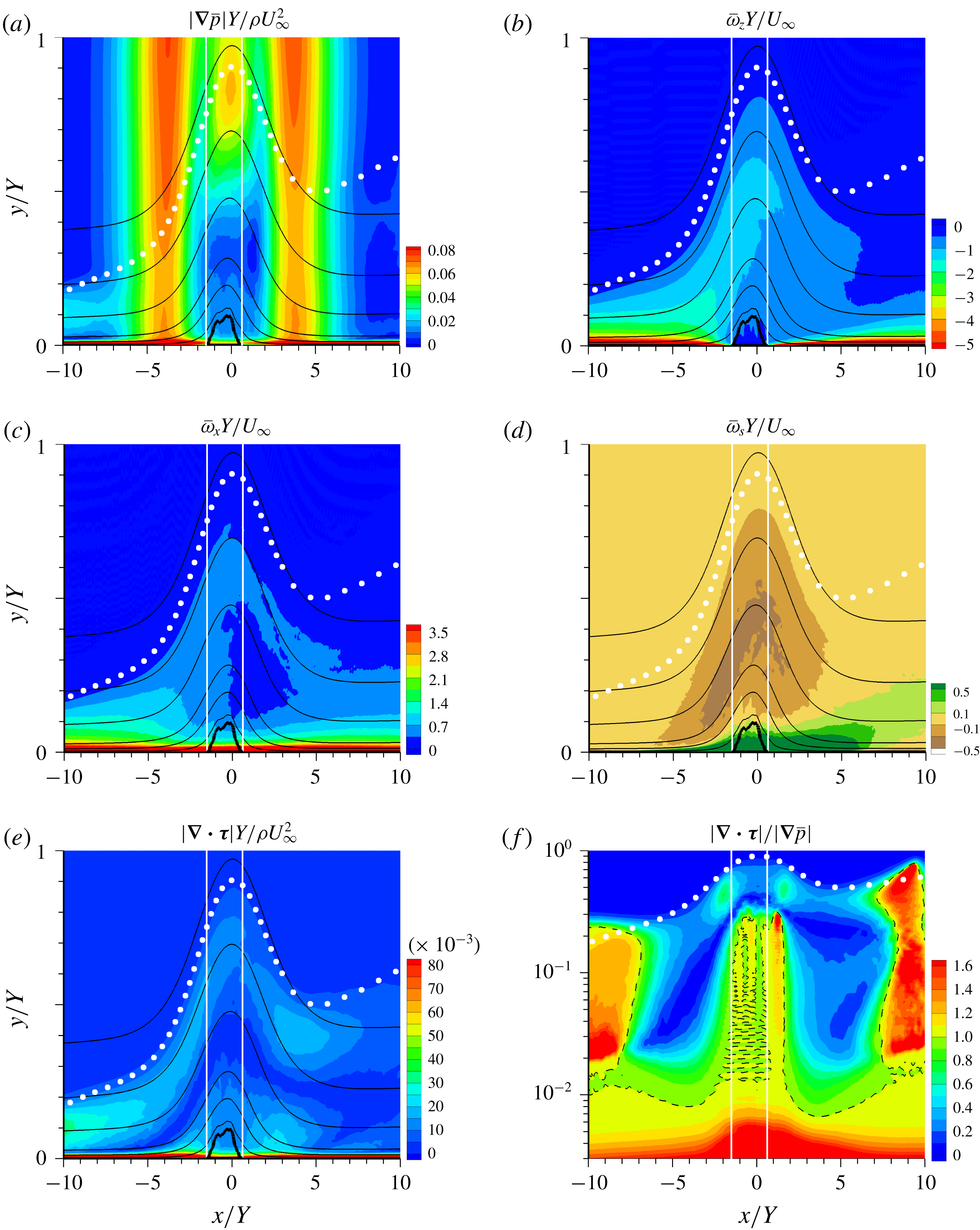
Case C35 contours of mean (a) pressure-gradient magnitude
 $|\unicode[STIX]{x1D735}\bar{p}|$
, (b) spanwise vorticity
 $\overline{\unicode[STIX]{x1D714}}_{z}$
, (c) chordwise vorticity
 $\overline{\unicode[STIX]{x1D714}}_{x}$
, (d) streamwise vorticity
 $\overline{\unicode[STIX]{x1D714}}_{s}$
, (e) Reynolds-stress-gradient magnitude
 $|\unicode[STIX]{x1D735}\boldsymbol{\cdot }\unicode[STIX]{x1D749}|$
and (f)
 $|\unicode[STIX]{x1D735}\boldsymbol{\cdot }\unicode[STIX]{x1D749}|/|\unicode[STIX]{x1D735}\bar{p}|$
ratio. Other symbols as in figure 8. Dark broken lines in (f) are
 $|\unicode[STIX]{x1D735}\boldsymbol{\cdot }\unicode[STIX]{x1D749}|=|\unicode[STIX]{x1D735}\bar{p}|$
contours. Norms of mean-pressure gradient and stress divergence respectively given by
 $|\unicode[STIX]{x1D735}\bar{p}|=[(\unicode[STIX]{x2202}\bar{p}/\unicode[STIX]{x2202}x_{i})(\unicode[STIX]{x2202}\bar{p}/\unicode[STIX]{x2202}x_{i})]^{1/2}$
, and
 $|\unicode[STIX]{x1D735}\boldsymbol{\cdot }\unicode[STIX]{x1D749}|=\unicode[STIX]{x1D70C}[(\unicode[STIX]{x2202}\overline{u_{i}^{\prime }u_{j}^{\prime }}/\unicode[STIX]{x2202}x_{j})(\unicode[STIX]{x2202}\overline{u_{i}^{\prime }u_{k}^{\prime }}/\unicode[STIX]{x2202}x_{k})]^{1/2}$
.

The similar behaviour for Cases C0 and C35 of the turbulence intensity and transport (production) efficiency exhibited in figure 8, near and above the separation, is compatible with the success of the IP in this region. However, the local maxima of
 $\mathit{k}$
and
 $\unicode[STIX]{x1D70F}_{prod}$
there potentially call into question our earlier proposal that success of the IP is correlated with negligible Reynolds stresses. However, even where it is most energetic, the turbulence does not fully control the evolution of the mean velocity in the non-ZPG regions. As the layer approaches separation, the APG becomes increasingly important in the RANS momentum equation, relative to the Reynolds-stress term. This can be seen from figure 9. Shown are
 $x$
–
 $y$
contours of the magnitude of the mean-pressure gradient
 $|\unicode[STIX]{x1D735}\bar{p}|$
, the mean spanwise
 $\overline{\unicode[STIX]{x1D714}}_{z}$
, chordwise
 $\overline{\unicode[STIX]{x1D714}}_{x}$
and streamwise
 $\overline{\unicode[STIX]{x1D714}}_{s}$
vorticity, as well as the Reynolds-stress divergence
 $|\unicode[STIX]{x1D735}\boldsymbol{\cdot }\unicode[STIX]{x1D749}|$
(see figure 9 legend for definition), and the ratio of the Reynolds-stress divergence to the pressure gradient
 $|\unicode[STIX]{x1D735}\boldsymbol{\cdot }\unicode[STIX]{x1D749}|/|\unicode[STIX]{x1D735}\bar{p}|$
.
First examining the inflow region, the large very-near-wall, wall-normal gradient of
 $|\unicode[STIX]{x1D735}\bar{p}|$
(figure 9
a) correlates well with the corresponding near-wall maximum of
 $|\unicode[STIX]{x1D735}\boldsymbol{\cdot }\unicode[STIX]{x1D749}|$
in figure 9(e), which is due to the wall-normal gradient of
 $\overline{v^{\prime }v^{\prime }}$
(White Reference White1991). In the outer layer, which is of most interest, the close correspondence between the mean streamlines and mean spanwise and chordwise vorticity contours points to a prominent role for inviscid transport in the APG region upstream of separation (figure 9
b,c). (The scales for the
 $\overline{\unicode[STIX]{x1D714}}_{x}$
and
 $\overline{\unicode[STIX]{x1D714}}_{z}$
contours have been adjusted so that the collateral state yields the same colours/contours. Note the non-zero spanwise near-wall shear across the separation zone in the
 $\overline{\unicode[STIX]{x1D714}}_{x}$
contours.) The growth of the streamwise vorticity
 $\overline{\unicode[STIX]{x1D714}}_{s}$
(i.e. the horizontal component parallel to
 $\boldsymbol{Q}_{\infty }$
) seen in figure 9(d) is the result of the well-known ‘inviscid skewing’ mechanism (Bradshaw Reference Bradshaw1987), which re-directs the cross-stream component
 $\overline{\unicode[STIX]{x1D714}}_{n}$
(normal to
 $\boldsymbol{Q}_{\infty }$
) in the
 $x$
–
 $z$
plane (see § 3.2.4, figure 10
a,b).
Figures 9(e) and especially 9(f) reveal the attenuation with
 $x$
of the Reynolds-stress divergence under the influence of the APG. The region in which the pressure gradient controls the mean-velocity evolution reaches quite close to the wall, and unexpectedly far upstream. (The broken curves in figure 9(f) trace the
 $|\unicode[STIX]{x1D735}\boldsymbol{\cdot }\unicode[STIX]{x1D749}|/|\unicode[STIX]{x1D735}\bar{p}|=1$
contours. Note the logarithmic wall-normal axis, used to clarify the near-wall behaviour.) This observation quantifies the above claim regarding the fading influence with
 $x$
of the turbulence, compared to the inviscid/pressure-gradient term, in the region where the IP becomes a better approximation.
We now turn to the output of the pressure-gradient/Reynold-stress imbalance, and examine the evolution of the mean-velocity profiles.
3.2.4 Mean velocity
Mean velocity for (a,c,e)
 $x<0$
and (b,d,f)
 $x>0$
for Case C35. (a,b) Component normal to
 $\boldsymbol{Q}_{\infty }$
,
 $\bar{u}_{n}=\bar{w}\cos \unicode[STIX]{x1D70E}-\bar{u}\sin \unicode[STIX]{x1D70E}$
: ▫,
 $y=\widetilde{\unicode[STIX]{x1D6FF}}_{995_{x}}$
. (c,d) Hodograph of chordwise and spanwise components. (e,f) Johnston (‘triangular’) plot (Bradshaw Reference Bradshaw1987), in components parallel
 $U_{\Vert }$
and orthogonal
 $U_{\bot }$
to local edge velocity
 $\boldsymbol{U}_{e}=\bar{u}_{e}\hat{\boldsymbol{e}}_{x}+\bar{w}_{e}\hat{\boldsymbol{e}}_{z}$
, where
 $\bar{u}_{e}(x)=\bar{u}(x,y=\widetilde{\unicode[STIX]{x1D6FF}}_{995_{x}})$
and
 $\bar{w}_{e}(x)=\bar{w}(x,y=\widetilde{\unicode[STIX]{x1D6FF}}_{995_{x}})$
. Shaded/grey curves/symbols, (in b,d,f)
 $x/Y=-8.5$
, and (in e) SWH prediction at
 $x/Y=-5$
,
 $-3$
and
 $-1.5$
. SWH prediction is
 $U_{\bot }=(1-U_{\Vert }/U_{e})\tan (2\unicode[STIX]{x1D703}_{SWH})$
, where
 $U_{e}=|\boldsymbol{U}_{e}|$
and
 $\unicode[STIX]{x1D703}_{SWH}=\unicode[STIX]{x1D70E}-\arctan (\bar{w}_{e}/\bar{u}_{e})$
(Bradshaw Reference Bradshaw1987).

The response of the swept ZPG boundary layer to the chordwise pressure gradient is illustrated in figure 10, in terms of the mean velocity. The left-hand side plots show the gradual departure, beginning from collateral conditions at
 $x/Y=-8.5$
(straight-line hodograph), up to the point of separation (solid magenta symbols). The right-hand-side plots reveal the FPG-to-ZPG recovery towards another collateral state, beginning from the mean reattachment station (solid green symbols). The open symbols in (a,b) mark the edge of the chordwise boundary layer,
 $y=\widetilde{\unicode[STIX]{x1D6FF}}_{995_{x}}$
. The introduction of mean three-dimensionality corresponds to growth of the velocity component (
 $\bar{u}_{n}$
) normal the plane containing the 2-D-ZPG velocity field (figure 10
a). Since the three-dimensionality is pressure driven, the cross-stream velocity profile has gradients
 $\unicode[STIX]{x2202}\bar{u}_{n}/\unicode[STIX]{x2202}y$
of opposite sign, above and below an off-the-wall maximum in
 $\bar{u}_{n}(y)$
. This leads to the triangular hodographs found in figure 10(c–f), which are characteristic of swept-wing 3DBLs (Gruschwitz Reference Gruschwitz1935; Johnston Reference Johnston1960). The primary source of the outer-layer gradient
 $\unicode[STIX]{x2202}\bar{u}_{n}/\unicode[STIX]{x2202}y$
is the inviscid-skewing mechanism mentioned earlier. (This mechanism is not present in shear-driven 3DBLs, such as those created by impulsive spanwise wall motion or in a plane channel by a sudden spanwise pressure gradient, since the resulting wall-normal gradient of spanwise velocity is of one sign.) The inviscid skewing mechanism assumes the wall-normal component of mean vorticity is zero in the outer layer (such that
 $\unicode[STIX]{x2202}\bar{u}_{s}/\unicode[STIX]{x2202}n=\unicode[STIX]{x2202}\bar{u}_{n}/\unicode[STIX]{x2202}s$
, where
 $s$
and
 $n$
are the streamwise and cross-stream coordinates), causing the horizontal mean vorticity and mean velocity to rotate about the
 $y$
axis through equal angles in opposite directions. This is consistent with the growth in
 $x$
of mean vorticity aligned with
 $\boldsymbol{Q}_{\infty }$
,
 $\overline{\unicode[STIX]{x1D714}}_{s}\approx \unicode[STIX]{x2202}\bar{u}_{n}/\unicode[STIX]{x2202}y$
, observed in the APG region of figure 9(d). Under these conditions, the outer-layer velocity closely satisfies the Squire–Winter–Hawthorne (SWH) relation (given in figure 10 legend). The good agreement between the DNS and the shaded linear curves/symbols in figure 10(e) demonstrates the excellent validity of the SWH relation for the region of APG-induced skewing. However, the practical impact of the outer-layer
 $\unicode[STIX]{x2202}\bar{u}_{n}/\unicode[STIX]{x2202}y$
, for example on the energetics and structure of the turbulence, appears to be rather limited. This is perhaps not surprising. Since inviscid skewing introduces ‘new’
 $\unicode[STIX]{x2202}\bar{u}_{n}/\unicode[STIX]{x2202}y$
that is actually ‘old’
 $\unicode[STIX]{x2202}\bar{u}_{s}/\unicode[STIX]{x2202}y$
, which goes to zero as
 $y\rightarrow \widetilde{\unicode[STIX]{x1D6FF}}_{995_{x}}$
, the cross-stream gradients in the outer layer will tend to be relatively weak compared to those nearer the wall. Further evidence of the minor role played by mean three dimensionality in the outer layer, compared to the impact of the APG, is provided in Coleman et al. (Reference Coleman, Rumsey and Spalart2019).
Profiles of magnitude
 $\bar{q}=(\bar{u}^{2}+\bar{w}^{2})^{1/2}$
and direction
 $\unicode[STIX]{x1D6FC}=\arctan (\bar{w}/\bar{u})$
for (a)
 $x<0$
and (b)
 $x>0$
for Case C35. Mean-velocity magnitudes and wall-normal distances are given in terms of wall units based on total wall stress, with
 $Q^{+}=\bar{q}/u_{\unicode[STIX]{x1D70F}}$
and
 $y^{+}=yu_{\unicode[STIX]{x1D70F}}/\unicode[STIX]{x1D708}$
, where
 $\unicode[STIX]{x1D70C}u_{\unicode[STIX]{x1D70F}}^{2}=\unicode[STIX]{x1D70F}_{w_{x}}^{2}+\unicode[STIX]{x1D70F}_{w_{z}}^{2}$
. Open symbols denote
 $\bar{w}/u_{\unicode[STIX]{x1D70F}_{z}}$
versus
 $yu_{\unicode[STIX]{x1D70F}_{z}}/\unicode[STIX]{x1D708}$
, where
 $\unicode[STIX]{x1D70C}u_{\unicode[STIX]{x1D70F}_{z}}^{2}=\unicode[STIX]{x1D70F}_{w_{z}}$
, at
 $\unicode[STIX]{x1D70F}_{w_{x}}\approx 0$
stations. Solid shaded/grey curves are from equation (16) of Luchini (Reference Luchini2018). Velocity profiles have been shifted five units in vertical scale above the one upstream, plotted below it. Horizontal mean-velocity direction given relative to surface shear angle
 $\unicode[STIX]{x1D6FC}_{0}=\arctan (\unicode[STIX]{x1D70F}_{w_{z}}/\unicode[STIX]{x1D70F}_{w_{x}})$
.

The profiles of magnitude (in wall units) and direction of the mean velocity in the
 $x$
–
 $z$
plane corresponding to the stations in figure 10 are shown in figure 11. Here we find an unexpected result, namely the lack of significant variation of the magnitude profiles
 $Q^{+}$
, scaled in terms of wall units based on the total shear stress. Each of the
 $Q^{+}$
profiles is similar to the high-Reynolds-number interpolant of Luchini (Reference Luchini2018) (solid shaded curves). This similarity occurs over the entire flow, through each of the ZPG-APG-FPG-ZPG regimes – oblivious to regions where the IP is and is not a reasonable approximation, including some with sizeable skewing away from the wall-stress direction – even at separation and reattachment. The closed and open symbols in figure 11 respectively represent the total and spanwise components at the
 $\unicode[STIX]{x1D70F}_{w_{x}}=0$
stations; while these must agree near the wall, they also match through the bulk of the inertial sublayer, to heights where the difference in the directions of mean velocity and surface shear approaches
 $20^{\circ }$
.
Mean-velocity profiles at (no symbols) separation and (symbols) reattachment in Stratford scaling for Cases C0 and C35:
 $\cdots \cdots$
, Stratford square-root law
 $U^{-}=B\sqrt{y^{-}}+C$
, with
 $(B,C)=(2.5,-2.2)$
(from Coleman et al.
Reference Coleman, Pirozzoli, Quadrio and Spalart2017), where
 $U^{-}=U/u_{p}$
,
 $y^{-}=yu_{p}/\unicode[STIX]{x1D708}$
and
 $u_{p}^{3}=\unicode[STIX]{x1D708}\,\text{d}(\bar{p}_{wall}/\unicode[STIX]{x1D70C})/\text{d}x$
.

Another view of the
 $\unicode[STIX]{x1D70F}_{w_{x}}=0$
profiles is given in figure 12, where the chordwise components are presented in the Stratford (Reference Stratford1959) scaling,
 $U^{-}$
versus
 $y^{-}$
(see legend for definitions). Although the Case C35 profiles at separation and reattachment tend to agree with each other, especially nearer the wall, they do not demonstrate the universal
 $\sqrt{y^{-}}$
behaviour observed for the
 $\unicode[STIX]{x1D70F}_{w_{x}}=0$
profiles from Case C0 (and from the other two unswept DNS considered earlier; see figure 10b of CRS18). The universal behaviour is shown by the dotted curve in figure 12, whose coefficients (
 $(B,C)=(2.5,-2.2)$
) derive from another series of DNS, of Couette–Poiseuille (CP) flow with zero mean skin friction on one wall (Coleman et al.
Reference Coleman, Pirozzoli, Quadrio and Spalart2017). One of the more surprising and noteworthy findings of CRS18 was that the same Stratford profile observed for parallel-flow turbulence driven by a constant pressure gradient above an extensive region of zero skin friction is also found at the separation and reattachment stations (only), in a spatially developing boundary layer with variable pressure gradients. The failure of universal Stratford similarity at the
 $\unicode[STIX]{x1D70F}_{w_{x}}=0$
locations is a formal violation of the IP, presumably due to the finite spanwise shear and turbulence stress, which prevents
 $u_{p}$
from being the only relevant velocity scale. However, in light of the collapse of the separation and reattachment profiles, and their order-of-magnitude agreement with the square-root law, this violation is most likely of little practical importance. Moreover, the amount of deviation from the universal profile by the chordwise Case C35 components is consistent with deviations induced by quite small, residual levels of skin friction found during the Coleman et al. (Reference Coleman, Pirozzoli, Quadrio and Spalart2017) CP DNS study. The previous and present DNS thus suggest that while it is well established, the universality of the Stratford scaling will likely not appear unless the assumptions upon which it is based are satisfied to a high level of accuracy.
4 Summary and closing comments
The subject has been DNS of a spatially developing turbulent boundary layer over a
 $35^{\circ }$
infinite swept surface under conditions leading to a small separation bubble. This case was designed to complement our earlier DNS of a turbulent separation bubble in an unswept flow. To isolate the effects of sweep, the chordwise component of the swept case is subjected to the same streamwise transpiration distribution as before. For both flows, care was taken to establish a fully developed ZPG state well upstream of the bubble; to facilitate the comparison, these ZPG layers were defined such that their chordwise (swept case) or streamwise (unswept) momentum thicknesses that would have ensued if the pressure gradient were not applied are the same at a common downstream station. If the Independence Principle (IP) were to be valid, this strategy would produce a flow whose projection onto the chordwise–wall-normal plane would be identical to the streamwise–wall-normal field of the unswept version. That the chordwise-projected and unswept fields differ over extensive regions demonstrates that the IP is in general not valid for swept turbulent boundary layers. In particular, the Kármán constant was altered by the cosine of the sweep angle, much as predicted by simply considering the log law in a collateral flow. We do, however, find that in the vicinity of the separation bubble, where the inviscid/pressure terms are more important than the turbulence-stress gradients, the IP is a fair approximation.
The manner in which the introduction of mean three-dimensionality affects the two-dimensional layer has been quantified. While the outer-layer inviscid skewing induced by the turning of the flow due to the misaligned pressure gradient is observed, and well predicted by the Squire–Winter–Hawthorne relationship in the outer layer (Bradshaw Reference Bradshaw1987), in the inner layer the magnitude of the mean velocity in local wall units is not far from the ZPG log law, even above the bubble, despite significant twisting of the mean-velocity vector. The mean three-dimensionality and outer-layer inviscid skewing have only a slight effect upon the structure of the turbulence (measured by the relationship of the components of the Reynolds-stress tensor and the efficiency of the turbulence energy transfer) compared with that of the adverse pressure gradient, which is active in both the present skewed and earlier unskewed layers. This is shown elsewhere, in Coleman et al. (Reference Coleman, Rumsey and Spalart2019). The Case C35 database, including thicknesses, skin friction, and mean-velocity and Reynolds-stress fields (available from https://turbmodels.larc.nasa.gov) is offered as a benchmark for other DNS, large-eddy simulation (LES) and RANS studies, and to guide turbulence theory and RANS modelling.
The ‘hybrid’ behaviour of the present swept flow, which merges a separated layer dominated by pressure/inertial effects (and as a consequence tends towards satisfying the IP) with a collateral turbulent ZPG layer up- and downstream of it (where the IP is clearly violated), represents a stiff turbulence-modelling challenge. In fact, contrary to our earlier supposition – that the presence of finite skin friction across the 3-D separation would ease the modelling burden – the challenge is comparable to that of the unswept case. Although swept-wing predictions of quantities such as the total skin friction should benefit from including a spanwise component that does not change sign (which presumably will in general be captured reasonably well), critical features such as the location of chordwise separation and its effect on the chordwise pressure distribution will remain elusive. This has been verified by applying multiple RANS models (using the code and approach described in CRS18) to the
 $35^{\circ }$
infinite-sweep geometry with Case C35 boundary conditions. For example, the chordwise component of skin-friction predictions (not shown here) given by the one-equation SA closure (Spalart & Allmaras Reference Spalart and Allmaras1994) and a recent Reynolds-stress transport (RST) scheme (Eisfeld, Rumsey & Togiti Reference Eisfeld, Rumsey and Togiti2016) are similar to the total
 $C_{f}$
predictions given by the same models applied to the unswept Case C0 flow in CRS18. In particular, both SA and RST yield mean separation locations – and
 $C_{f_{x}}$
variations upstream of it – that are quite close to each other, and slightly earlier than the DNS separation station (cf. figure 15 of CRS18). Furthermore, although their
 $C_{f_{x}}$
variations have the same shape as the DNS downstream of reattachment (recall the absence of the delayed recovery for Case C35, observed in figure 6
b), the RST scheme still reattaches and recovers towards ZPG conditions sooner than SA and especially sooner than the DNS. These observations point to the value of further RANS-model development applied to the APG-induced separation of unswept flat-plate boundary layers, over a range of conditions. The prediction of separation is viewed as a central issue by the Aerospace industry and NASA (Slotnick et al.
Reference Slotnick, Khodadoust, Alanso, Darmofal, Gropp, Lurie and Mavriplis2014).
In CRS18, it was suggested the Stratford mean-velocity scaling might be a worthwhile RANS development benchmark: a ‘perfect’ model would match it just like it matches the log law. In this study, the benefits are not so obvious. On one hand, the Stratford scaling appears to be rather fragile, in that either fairly low values of spanwise shear above the separation region (as found here) or residual (chordwise) skin friction (as found in the Couette–Poiseuille DNS of Coleman et al. (Reference Coleman, Pirozzoli, Quadrio and Spalart2017) drive the flow away from square-root behaviour, or disturb the universality of its constants. Unlike for the streamwise component of the unswept flow (CRS18), the chordwise component of the 3-D velocity profile at separation and reattachment is not accurately represented by the universal square-root idealization. On the other hand, the Case C35 spanwise shear above the bubble does not lead to chordwise velocity profiles that are vastly different from the Stratford idealization, which may imply that constraining a RANS model to satisfy the Stratford profile for the purely 2-D
 $C_{f}=0$
state might lead to improvements under more general conditions.
The present study is being extended by a new DNS of unswept separation, similar to Case C0 but with transpiration of one sign, such that there is no FPG downstream of the bubble (cf. Wu, Meneveau & Mittal Reference Wu, Meneveau and Mittal2019).
As of now we have no proposals to modify the RANS models to better agree with either the C0 or the C35 flow. Improving models in one area without sacrificing their useful performance in other areas is a very slow process. The dataset could also be a basis to test LES approaches, especially with wall modelling; the Reynolds number, although moderate, appears sufficiently high for this.
Acknowledgements
This research was sponsored by the NASA Transformational Tools and Technologies (TTT) Project of the Transformative Aeronautics Concepts Program under the Aeronautics Research Mission Directorate. Computations were performed on resources provided by the NASA Advanced Supercomputing (NAS) Division. Dr M. Strelets made useful comments.