


1. Introduction
Insurance enables policyholders to transfer part of their losses to insurers in exchange for a premium, with insurers covering the transferred losses. Insurers price insurance contracts with premiums that reflect the underlying risk, following a consistent premium principle. While greater insurance coverage reduces the policyholder’s risk exposure, it also leads to a higher premium. Therefore, determining the optimal amount of insurance typically involves a trade-off for both parties. An insurance contract is finalized when the policyholder agrees to its terms. Since the work of Borch (Reference Borch1960) and Arrow (Reference Arrow1963), numerous papers in the literature have studied related topics. For instance, Cui et al. (Reference Cui, Yang and Wu2013), Assa (Reference Assa2015), Zhuang et al. (Reference Zhuang, Weng, Tan and Assa2016), and Cheung et al. (Reference Cheung, Chong and Lo2019) study preferences represented by minimizing a distortion risk measure, such as value-at-risk (VaR) and tail value-at-risk (TVaR). Wang et al. (Reference Wang, Young and Panjer1997) explore the properties of distortion risk measures in insurance, highlighting the ability to capture policyholders’ risk preferences and insurers’ pricing strategies.
This paper studies the insurance problem when the policyholder incorporates prevention efforts to influence the loss distribution. Specifically, we analyze the equilibrium between the policyholder and multiple insurers in an effort-dependent loss prevention setting, where insurers cannot observe the policyholder’s actual effort level directly.
Traditionally, the policyholder’s loss is modeled as a fixed random variable, with contracts designed to optimize risk sharing under a given premium principle. However, in many cases, the policyholder can seek to affect the loss amount through prevention actions (Dionne et al., Reference Dionne, Doherty and Fombaron2000; Doherty and Smetters, Reference Doherty and Smetters2005; Rees and Wambach, Reference Rees and Wambach2008). These actions, collectively referred to as prevention efforts, introduce complexity because effort influences the loss distribution while remaining unobservable to the insurer. To address this, insurers must design contracts so that the premium is based on a “standard" level of effort that, in equilibrium, the policyholder is induced to choose.
The framework developed in this paper considers a setting in which the policyholder’s effort modifies the loss distribution, with higher effort levels reducing the probability of large losses. Insurers compete under full competition and have no monopoly power in the market; they earn zero risk-adjusted profit in equilibrium. The policyholder, on the other hand, seeks to minimize an objective function based on a risk measure by choosing insurance coverage and adjusting the effort level. Effort incurs a cost modeled as a strictly convex function, reflecting the increasing marginal costs associated with higher effort levels. Meanwhile, all insurers set the premium based on a common belief (benchmark) about effort; realized effort is not observable. The equilibrium of this interaction is characterized by a premium corresponding to a benchmark effort level chosen by the insurers. Such a benchmark effort level coincides with the actual effort of the policyholder, and the policyholder selects the effort that minimizes the risk measure given losses, insurance coverage, and cost of effort.
1.1. Relevance of research
This study contributes to the literature on insurance optimization by incorporating prevention efforts. Recently, Bensalem et al. (Reference Bensalem, Hernández Santibáñez and Kazi-Tani2020) study an equilibrium model in a Stackelberg setup, where the insurer (seller) sets prices through loading factors, and the policyholder (buyer) selects the optimal level of observable prevention effort to minimize the risk measure. Other developments focus on optimal (re)insurance strategies, considering scenarios involving either low or high risks, with probabilities of occurrence assigned to each scenario. Additionally, in economics, related topics are often studied using the principle of utility maximization (Akerlof, Reference Akerlof1970; Doherty and Schlesinger, Reference Doherty and Schlesinger1990; Winter, Reference Winter and Dionne2000; Doherty and Smetters, Reference Doherty and Smetters2005; Ligon and Thistle, Reference Ligon and Thistle2005). This paper expands on these studies by analyzing loss distributions that depend on prevention efforts. Prevention efforts are a critical yet underexplored aspect of risk management, as they influence both the severity and frequency of losses (Ehrlich and Becker, Reference Ehrlich and Becker1972; Rees and Wambach, Reference Rees and Wambach2008). By explicitly modeling prevention efforts, this paper captures a more realistic framework where the policyholder can take actions to mitigate risks but faces cost–benefit trade-offs at the same time.
From a practical perspective, this paper highlights challenges faced by insurers in designing contracts under asymmetric information. Insurers cannot directly observe the policyholder’s effort level and operate under full competition. This aligns with real-world scenarios in which policyholders may not truthfully disclose information to an insurer, leading to potential inefficiencies in risk sharing. Understanding how prevention efforts influence equilibrium provides insights into designing contracts that align incentives, minimize moral hazard, and achieve optimal outcomes for both parties.
1.2. Literature review
Insurance contract optimization is a central topic in risk management. Traditional frameworks often assume fixed loss distributions, where insurance contracts are designed to optimize the policyholder’s expected utility of terminal wealth under a given premium principle. However, more recent studies have incorporated various factors, such as prevention efforts, moral hazard, and asymmetric information, to better reflect real-world complexities (Gauchon et al., Reference Gauchon, Loisel, Rullière and Trufin2020; Bensalem et al., Reference Bensalem, Hernández Santibáñez and Kazi-Tani2020; Boonen and Zhang, Reference Boonen and Zhang2022).
Asymmetric information significantly impacts the design of insurance contracts. Although prevention efforts help reduce risk, they are typically unobservable to the insurer. This lack of transparency forces insurers to design contracts that induce optimal policyholder behavior. Doherty and Schlesinger (Reference Doherty and Schlesinger1990) and Ligon and Thistle (Reference Ligon and Thistle2005) show that unobservable actions by the policyholder can lead to inefficiencies in risk sharing between the two parties. From the perspective of the policyholder, Bensalem et al. (Reference Bensalem, Hernández Santibáñez and Kazi-Tani2023) study prevention efforts in an insurance model in continuous time, where the objective is to maximize the expected utility of terminal wealth. Moreover, Cheung et al. (Reference Cheung, Chong and Lo2019) and Boonen and Zhang (Reference Boonen and Zhang2022) examine the role of a monopolistic insurer by selecting indemnity functions and premium principles under asymmetric information about the policyholder’s risk preferences. They design the contract to minimize the distortion caused by asymmetric information. Gauchon et al. (Reference Gauchon, Loisel, Rullière and Trufin2020) and (Reference Gauchon, Loisel, Rulliere and Trufin2021) study prevention in insurance in a classical risk model. Their focus is on the prevention strategies that are organized and paid for by the insurer, where the insurance contracts are treated as given. In a general risk-sharing context with n peers, moral hazard and prevention efforts are studied by Von Bieberstein et al. (Reference Von Bieberstein, Feess, Fernando, Kerzenmacher and Schiller2019).
1.3. Main contributions
Although significant progress has been made in understanding prevention efforts and asymmetric information in insurance contract design, several gaps remain. As mentioned, many current studies assume either static or predetermined loss distributions; consequently, the literature on settings in which the policyholder can directly affect the loss distribution through effort remains limited. Furthermore, the equilibrium interaction between policyholders and insurers in the presence of prevention efforts has been relatively unexplored in the context of distortion risk measures, particularly when effort is unobservable to the insurer.
This paper extends the work of Bensalem et al. (Reference Bensalem, Hernández Santibáñez and Kazi-Tani2020), Seog and Hong (Reference Seog and Hong2024), and Li et al. (Reference Li, Wang and Zhang2026) by explicitly modeling prevention efforts as a key factor that affects loss distributions. Bensalem et al. (Reference Bensalem, Hernández Santibáñez and Kazi-Tani2020) focus on how prevention efforts affect self-insurance and self-protection and the decision to buy proportional insurance with observable effort and also discuss the interaction between insurance buyers and sellers. Seog and Hong (Reference Seog and Hong2024) study moral hazard problems with prevention efforts for binary loss distributions in a utility-based setting. Moreover, Li et al. (Reference Li, Wang and Zhang2026) study self-protection with fully observable prevention efforts using distortion risk measures and analyze optimal proportional insurance decisions under convex premium principles. In addition to those papers, our paper makes the following distinct contributions:
-
1. General indemnity and novel modeling of efforts: This study does not restrict indemnities to proportional forms. Proportional indemnities imply that the policyholder and insurer share losses in a fixed proportion. While this simplifies the analysis, it does not fully capture the complexity of real-world insurance contracts. Instead, we allow for general indemnity structures, in which the indemnity is modeled by a function, which provides more flexibility. By allowing for general indemnities, this paper provides a more realistic analysis of contracts and enables the determination of optimal equilibria without the constraints of proportional indemnity structures. In addition, the prevention effort dynamically modifies the survival function of the loss distribution, where higher effort reduces the probability of large realizations of the risk. In this setup, a cost–benefit trade-off is reflected in the determination of the policyholder’s optimal effort level.
-
2. Equilibrium concept with effort matching: A novel contribution of this paper is the introduction of an equilibrium concept in which the insurers’ effort expectations align with the policyholder’s actual effort. This alignment ensures that insurers can design contracts to induce the policyholder to select an optimal effort level via a consistency (fixed-point) condition between the insurers’ pricing benchmark and the policyholder’s best response. The paper provides sufficient conditions for the existence of this equilibrium and analyzes premium pricing, effort levels, and risk sharing within this framework.
-
3. Asymmetric information: Under asymmetric information, insurers cannot observe the policyholder’s effort level directly. This study demonstrates how premiums can serve as a mechanism to induce optimal behavior from the policyholder and ensure efficient risk sharing under incomplete information about effort levels. In addition, the paper provides a detailed analysis of how parameters (i.e., loading factors, effort expectations, and cost functions) affect equilibrium effort levels. For specific cases, such as exponential loss distributions, we derive explicit solutions and use comparative statics to offer practical insights for contract design.
-
4. Symmetric information and moral hazard: While the focus is on asymmetric information, this paper also considers symmetric information, where insurers directly observe the policyholder’s effort level. Under symmetric information, insurers design contracts without anticipating a strategic response in the effort level. Instead, the insurer takes the actual effort as given and prices accordingly. The symmetric case enables a comparison between symmetric and asymmetric information solutions, highlighting how asymmetric information introduces moral hazard and inefficiencies in effort decisions. Specifically, our results indicate how insurers should adjust the insurance contract to mitigate inefficiencies.
By addressing the above features, this paper provides a comprehensive and realistic analysis of insurance contracts. It can lead to an effective risk-sharing arrangement, as it provides a framework that models prevention efforts, generalizes indemnity structures, and establishes equilibrium conditions.
1.4. Structure of the paper
Section 2 discusses the problem formulation and assumptions used in this paper. Sections 3 and 4 study the cases in which the policyholder’s distortion risk measures are VaR and TVaR, respectively. Section 5 shows results under a general strictly concave distortion function. The sections above assume that prevention effort is unobservable to insurers. Section 6 studies the setting under symmetric information about prevention efforts, showing that the policyholder’s objective value is generally strictly better under symmetric information. Auxiliary derivations are provided in the Appendix.
2. Problem formulation
We study a market in which a potential policyholder faces a nonnegative random loss X. We assume that all random variables are defined on a fixed atomless probability space
 $(\Omega, \mathcal{F}, \mathbb{P})$
. Let
 $\mu$
be the Lebesgue measure on
 $\mathbb{R}_+\;:\!=\; [0, \infty)$
. Let
 $\mathbb{R}_{++}\;:\!=\; (0, \infty)$
, and let
 $\mathbf{1}_A(s)$
denote the indicator function such that
 $\mathbf{1}_A(s) = 1$
for
 $s \in A$
and
 $\mathbf{1}_A(s) = 0$
for
 $s \notin A$
. The cumulative distribution function and survival function of a random variable X are denoted by F and S, respectively. The quantile of X at level
 $p \in [0, 1]$
is the generalized inverse
 $F^{-1}(p) \;:\!=\; \inf\{x \in \mathbb{R}_+ \mid F(x) \geq p\}$
.
2.1. Loss distributions and survival functions
The policyholder seeks to transfer some of the risk to multiple insurers. Assume that the policyholder can choose an effort level
 $e \in [0, 1]$
and incurs a cost c(e). Both the policyholder and insurers know how the loss distribution depends on effort. However, the effort level selected by the policyholder is unobservable to insurers. Both parties know the mapping
 $e\to X_e$
and hence
 $S_e$
, but insurers cannot condition the premium on the realized value of e. This assumption creates a classical moral hazard scenario: insurers must form beliefs about the policyholder’s effort when pricing the contract, and the premium cannot be determined based on the realized effort. In addition, greater effort reduces the likelihood of large losses by shifting the loss distribution. Let
 $X_e$
denote the loss under effort level e. We take two loss distributions as primitives:
 \[ \begin{cases} X_0, \quad\text{the loss under no effort ($e=0$), with survival function $S_0(z)=\mathbb{P}(X_0\gt z)$,}\quad z\geq0.\\[5pt] X_1, \quad\text{the loss under full effort ($e=1$), with survival function $S_1(z)=\mathbb{P}(X_1\gt z)$,}\quad z\geq0. \end{cases}\]
Here,
 $S_0$
corresponds to the loss distribution under no effort (worst case), and
 $S_1$
corresponds to the loss distribution under full effort (best case). We assume
 $S_0(z)\geq S_1(z)$
for all
 $z\geq0$
. If the corresponding distributions admit densities, we denote them by
 $f_0$
and
 $f_1$
, respectively.
For any effort level
 $e\in[0,1]$
, we model the survival function of
 $X_e$
as a convex combination of
 $S_0$
and
 $S_1$
:
 \[ S_e(z) = eS_1(z) + (1 - e)S_0(z), \quad\text{ for all } z\geq0.\]
Let
 $M=\sup\{z\in\mathbb{R}_+|S_0(z)\gt0\}$
, which may be infinite. Thus, the support of
 $X_e$
is contained in [0, M) if
 $M\lt\infty$
, and in
 $[0,\infty)$
otherwise. For fixed e,
 $S_e(z)$
is nonincreasing in z; for fixed z,
 $S_e(z)$
is nonincreasing in e. To simplify the analysis, we make an additional assumption about the survival functions
 $S_0$
and
 $S_1$
.
Assumption 2.1. The survival functions
 $S_0(z)$
and
 $S_1(z)$
satisfy
 \[S_0(0)=S_1(0)\;:\!=\; 1-p_0,\]
where
 $p_0\in[0,1)$
and are twice continuously differentiable on
 $\mathbb{R}_{++}$
. The corresponding densities
 $f_0$
and
 $f_1$
are positive on (0, M).
Under Assumption 2.1, it holds that
 $p_0=\mathbb{P}(X_e=0)$
. Our model assumes that
 $p_0$
is exogenous and remains unchanged regardless of effort. In other words, the effort level will only affect the distribution when a loss occurs. The survival function is discontinuous at 0 when
 $p_0\neq0$
. This reflects real-world applications in catastrophe insurance, where prevention efforts cannot influence the probability of a loss but can mitigate the magnitude of the loss if a catastrophe occurs (e.g., earthquake damage in home insurance). This implies that our focus is on self-insurance and not self-protection. Moreover, Assumption 2.1 guarantees that for
 $z\in(0,M)$
and
 $e\in[0,1]$
, the value
 $\partial S_e(z)/\partial z$
always exists and is continuous. Additionally, we allow for a discrete event with positive probability, but only at
 $X_e=0$
. Note that differentiability of the survival function on
 $\mathbb{R}_{++}$
implies that the loss variable has a continuous distribution on (0, M), with a possible atom at 0.
2.2. Indemnity and marginal indemnity functions
The admissible set of indemnity functions is defined as follows:
 \[ \mathcal{I} = \{I\;:\;\mathbb{R}_+\to\mathbb{R}_+\mid I(0)=0,0\leq I(x)-I(y)\leq x-y, 0\leq y\leq x\}.\]
For any
 $I\in\mathcal{I}$
, both I(x) and
 $x-I(x)$
are nondecreasing. The set
 $\mathcal I$
consists of indemnities that satisfy the so-called no-sabotage condition. For more detailed discussions, we refer to Huberman et al. (Reference Huberman, Mayers and Smith1983) and Denuit and Vermandele (Reference Denuit and Vermandele1998).
The functions in
 $\mathcal I$
are 1-Lipschitz, and thus absolutely continuous. Therefore, there exists a Lebesgue-measurable function
 $h\;:\;\mathbb{R}_+ \to [0,1]$
such that:
 \begin{equation} I(x)=\int_0^x h(z)\, dz, \quad x \in \mathbb{R}_+,\end{equation}
where h is called the marginal indemnity function of I (Assa, Reference Assa2015).
2.3. Distortion risk measure
A distortion function
 $g\;:\;[0,1] \to [0,1]$
is a nondecreasing, left-continuous function such that
 $g(0)=0$
and
 $g(1)=1$
. The set of all distortion functions is denoted by
 $\mathcal{G}_d$
, and the subset of distortion functions that are concave on [0, 1] is denoted by
 $\mathcal{G}_{cv}$
. Note that
 $\mathcal{G}_{cv} \subset \mathcal{G}_d$
.
Definition 2.1. A distortion risk measure
 $\rho_g$
of a random variable Z with distortion function
 $g \in \mathcal{G}_d$
is defined as:
 \begin{equation*} \rho_g(Z) = \int_0^{\infty}g(\mathbb{P}(Z\gt t))\,dt + \int^0_{-\infty}[g(\mathbb{P}(Z\gt t))-1]\,dt, \end{equation*}
provided that the integrals exist.
A distortion risk measure
 $\rho_g$
is convex if
 $g \in \mathcal{G}_{cv}$
. Convex distortion risk measures preserve second-order stochastic dominance (Wang et al., Reference Wang, Young and Panjer1997) and imply aversion to mean-preserving spreads (Yaari, Reference Yaari1987). An example of a nonconvex distortion risk measure is VaR.
Definition 2.2. The VaR of a nonnegative random variable Z at confidence level
 $\alpha \in (0,1)$
is defined as:
 \[ VaR_{\alpha}(Z)\;:\!=\;\inf\{z \in \mathbb{R}_+\;:\; \mathbb{P}(Z\leq z) \geq \alpha\}=F^{-1}_Z(\alpha), \]
where
 $F^{-1}_Z$
is the quantile function of random variable Z. The VaR is a distortion risk measure with distortion function
 $g(t)=\mathbf{1}_{(1-\alpha,1]}(t)$
.
Next, we define TVaR, a convex distortion risk measure.
Definition 2.3. The TVaR of a nonnegative random variable Z at a confidence level
 $\alpha\in(0,1)$
is defined as:
 \begin{equation*} TVaR_{\alpha}(Z)\;:\!=\;\frac{1}{1-\alpha}\int_{\alpha}^1 VaR_{\gamma}(Z)\,d\gamma. \end{equation*}
TVaR is a distortion risk measure with distortion function
 $g(t)=\min\left\{1,\frac{t}{1-\alpha}\right\}$
.
2.4. Competitive insurers and indifference pricing
We treat all insurers in the insurance market as fully competitive. There is a large pool of insurers, each of negligible size, so that none of them can influence the price. The policyholder may purchase coverage from multiple insurers. As a result, insurers are effectively price takers: they can only decide whether to offer contracts to the policyholder, who is always free to switch to other insurers in the market. In equilibrium, active insurers must charge a common premium that yields zero risk-adjusted profit. This is the standard zero-profit condition in a traditional fully competitive insurance market setup (Rothschild and Stiglitz, Reference Rothschild and Stiglitz1978).
All insurers are assumed to have identical objective functions. Each insurer evaluates losses using the same comonotonic additiveFootnote
1
distortion risk measure
 $\rho_{g_i}$
with distortion function
 $g_i\in\mathcal G_d$
, and faces the same administrative costs. Insurers understand the mapping
 $e\to X_e$
(and thus
 $e\to S_e$
) but cannot observe the actual effort chosen by the policyholder. They form a common pricing benchmark
 $e^*\in[0,1]$
and price as if losses follow
 $X_{e^*}$
. Given
 $e^*$
, for any quoted premium
 $\tilde\Pi\geq 0$
, an insurer that offers indemnity I evaluates
 \begin{equation}\rho_{g_i}(\!-\!W+I(X_{e^*})-\tilde\Pi+C(I(X_{e^*}))).\end{equation}
where
 $W\in\mathbb{R}$
is initial wealth and
 $C(I(X_{e^*}))=\theta\rho_{g_i}(I(X_{e^*}))$
for
 $\theta\geq0$
. Here, C represents the administrative cost that is assumed to be proportional to the risk measure of the indemnity (Boonen and Zhang, Reference Boonen and Zhang2022).Footnote
2
Under full competition, equilibrium premiums are characterized by the indifference condition, taking into account the policyholder’s optimal decision regarding the effort and indemnity function (which we will discuss in Section 2.5). The objective function in (2) is common knowledge to both insurers and the policyholder. In particular,
 $g_i$
is not a decision variable of the insurer in our model, as it describes the insurer’s given risk preferences.
Because the policyholder’s realized effort is unobservable, insurers cannot condition premiums on realized effort and must therefore price contracts based on a belief about effort, denoted by
 $e^*\in[0,1]$
. This is standard in hidden-action (moral-hazard) models of insurance and contracting, where pricing and contract terms depend on beliefs, and equilibrium requires those beliefs to be consistent with the agent’s optimal response (Holmstrom, Reference Holmstrom1979; Shavell, Reference Shavell1979; Arnott and Stiglitz, Reference Arnott and Stiglitz1988). Accordingly, we focus on a belief-consistent equilibrium: given premiums computed at
 $e^*$
, the policyholder chooses effort e optimally, and in equilibrium beliefs are correct, i.e.,
 $e^*=e$
.
If all insurers have the same beliefs
 $e^*$
, then full competition yields indifference pricing (Aase, Reference Aase1993; Carmona, Reference Carmona2008). That is, the premium is determined by the solution to
 \begin{equation} \rho_{g_i}(\!-\!W+I(X_{e^*})-\tilde\Pi+C(I(X_{e^*})))=\rho_{g_i}(\!-\!W).\end{equation}
By translation invariance of
 $\rho_{g_i}$
,Footnote
3
this yields
 \begin{align}\nonumber \tilde \Pi&=\Pi_{g_i}(I(X_{e^*}))\;:\!=\; (1+\theta)\rho_{g_i}(I(X_{e^*}))=(1+\theta)\int_0^{M}g_i(\mathbb{P}(I(X_{e^*})\gt z))\, dz\\[5pt] &=(1+\theta)\int_0^{M}g_i(S_{e^*}(z))h(z)\, dz, \end{align}
where h is the marginal indemnity function of I (see (1)), and the second equation is derived from Cheung and Lo (Reference Cheung and Lo2017).
For any fixed indemnity, the policyholder purchases from the insurer(s) quoting the lowest premium; insurers quoting a strictly higher premium receive zero demand. In the next proposition, we show that in equilibrium all insurers are indeed indifferent between selling or not selling insurance.
Proposition 2.1. Suppose the policyholder chooses the lowest available premium for any given coverage. If all other insurers quote
 $\Pi_{g_i}(I(X_{e^*}))$
and the policyholder’s best response satisfies
 $e=e^*$
, then matching
 $\Pi_{g_i}(I(X_{e^*}))$
is an optimal response for any insurer, and at this premium the insurer’s risk measure equals
 $-W$
.
Proof. Let
 $e^*$
be the benchmark effort and suppose the policyholder’s best response is
 $e=e^*$
. Fix indemnity I. Consider a deviating insurer that quotes
 $\tilde \Pi$
, while all other insurers quote
 $\Pi_{g_i}(I(X_{e^*}))$
. Given that
 $C(I(X_{e^*}))=\theta\cdot\rho_{g_i}(I(X_{e^*}))$
and by the translation invariance property of the distortion risk measure
 $\rho_{g_i}$
, for this specific insurer charging
 $\tilde \Pi$
, we have
 \begin{equation} \rho_{g_i}(\!-\!W+I(X_{e^*})-\tilde \Pi+C(I(X_{e^*}))) = \rho_{g_i}(\!-\!W) + (1+\theta)\rho_{g_i}(I(X_{e^*})) - \tilde \Pi. \end{equation}
We now compare three cases for
 $\tilde \Pi$
:
-
•
 $\tilde\Pi = \Pi_{g_i}(I(X_{e^*}))$
. Substituting the expression into (5) gives: Thus, at the premium
\[ \rho_{g_i}(\!-\!W+I(X_{e^*})-\tilde\Pi+C(I(X_{e^*})))= -W+(1+\theta)\rho_{g_i}(I(X_{e^*}))-(1+\theta)\rho_{g_i}(I(X_{e^*}))= -W. \]
$\Pi_{g_i}(I(X_{e^*}))$
, the insurer’s risk measure equals
$-W$
, which is exactly the value of not selling any insurance (the terminal loss position
$-W$
). This is the indifference pricing condition, where the insurer is indifferent between participating and not participating in the insurance market.
-
•
$\tilde\Pi \lt \Pi_{g_i}(I(X_{e^*}))$
. Here, the insurer offers a strictly lower premium than other insurers. Under full competition, the policyholder strictly prefers this contract, so the deviator attracts the corresponding business. Also, from (5), we have: and thus
\[ (1+\theta)\rho_{g_i}(I(X_{e^*})) - \tilde\Pi \gt 0, \]
Therefore, any premium lower than the competitive premium leads to a higher value of the risk measure than
\[ \rho_{g_i}(\!-\!W + I(X_{e^*}) - \tilde\Pi + C(I(X_{e^*}))) \gt -W. \]
$-W$
. In other words, the insurer is strictly worse off than if it had either not sold any insurance or matched the indifference premium. A rational insurer will therefore not choose a premium
$\tilde\Pi$
below
$\Pi_{g_i}(I(X_{e^*}))$
.
-
•
$\tilde\Pi \gt \Pi_{g_i}(I(X_{e^*}))$
. Here, the policyholder prefers the contract offered by other insurers because the premium is strictly lower. The insurer sells no insurance, and its final position remains at
$-W$
. This is the same risk measure as if it had charged
$\Pi_{g_i}(I(X_{e^*}))$
and sold the contract. Thus, choosing a premium
$\tilde\Pi \gt \Pi_{g_i}(I(X_{e^*}))$
does not yield a better outcome than matching the competitive premium and, under the usual convention that insurers are willing to transact when indifferent, such a deviation is weakly dominated by
$\tilde\Pi = \Pi_{g_i}(I(X_{e^*}))$
.


Therefore, given all other insurers price at
 $\Pi_{g_i}(I(X_{e^*}))$
, it is optimal for a new insurer to choose the same premium
 $\Pi_{g_i}(I(X_{e^*}))$
. At this premium, the insurer’s risk measure equals
 $-W$
, and it is indifferent between selling and not selling. This completes the proof.
Proposition 2.1 characterizes indifference pricing in a fully competitive market with hidden effort, under a belief-consistent equilibrium where the pricing benchmark equals the policyholder’s optimal effort. At a belief-consistent equilibrium (
 $e=e^*$
), all insurers quote
 $\Pi_{g_i}(I(X_e))$
. It shows that, taking all other insurers’ behavior as given, the best response for a specific insurer is to quote exactly this premium,
 $\Pi_{g_i}(I(X_e))$
, under which the risk measure becomes
 $-W$
. It is equal to the value of not selling any insurance, so it earns zero risk-adjusted profit and is indifferent between participating and not participating in the market. By comonotonic additivity of
 $\Pi_{g_i}$
, the insurers can be collectively represented by a single representative insurer, using the same premium principle
 $\Pi_{g_i}(I(X_e))$
(see Boonen et al., Reference Boonen, Tan and Zhuang2016). Boonen et al. (Reference Boonen, Tan and Zhuang2016) show that the aggregate indemnity assigned to the representative insurer can be allocated among the insurers in any comonotonic way. In the remainder of this paper, we focus only on this single representative insurer.
2.5. Policyholder’s objective function and the optimization problem
Assume that the policyholder is endowed with a distortion function
 $g_p\in\mathcal{G}_{d}$
. The optimization problem for the policyholder is given as follows:
 \begin{equation} \inf_{I\in\mathcal I,\, e\in[0,1]}\rho_{g_p}(X_e-I(X_e)+\Pi_{g_i}(I(X_{e^*})))+c(e),\end{equation}
where
 $g_i\in\mathcal{G}_d$
,
 $\theta\geq0$
are common knowledge to the policyholder,
 $I\in\mathcal{I}$
, and
 $\Pi_{g_i}$
, the general premium principle as in Cheung and Lo (Reference Cheung and Lo2017) mentioned in Section 2.4, is disclosed to the policyholder. In addition,
 $e^*\in[0,1]$
, determined by the insurer, is also known to the policyholder, and
 $c(e) = \gamma\cdot c_0(e)$
for
 $\gamma\gt0$
is a cost function.
Zero effort is assumed to be costless:
 $c_0(0)=0$
, and the marginal cost of effort at zero effort is also assumed to be zero:
 $c_0'(0)=0$
, meaning that small increases in effort around zero effort have minimal cost. Moreover, as effort approaches its maximum (
 $e\to1$
), the marginal cost of additional effort increases rapidly, reflecting the scarcity or higher cost of resources needed to further increase effort. This is consistent with the diminishing returns intuition in economics, together with the effect of effort on the loss distribution, since when the effort is already high, further loss reduction is achieved only at higher cost. This circumstance discourages the policyholder from opting for
 $e=1$
. Specifically, we assume that the function
 $c_0$
satisfies the following properties:
 \begin{equation} c_0(0)=0,\quad \lim_{e\rightarrow 1}c_0(e)=\infty, \quad c_0'(0)=0, \quad c_0'(e)\geq0, \text{ and } c_0''(e)\gt0, \quad\text{ for all }e\in[0,1).\end{equation}
The structure
 $c(e) = \gamma c_0(e)$
is common in previous literature, where effort costs are captured by a given function and multiplied by a scalar (Chen, Reference Chen2005; Zhang and Xu, Reference Zhang and Xu2017; Macho-Stadler and Pérez-Castrillo, Reference Macho-Stadler and Pérez-Castrillo2021). We want the function
 $c_0$
to determine the shape of the cost function (in particular, nondecreasing and strictly convex), while the parameter
 $\gamma$
scales the cost of effort.
In addition, economically speaking,
 $\gamma$
can be interpreted as a measure of the policyholder’s cost of effort and as a parameter controlling the marginal cost of effort, as a larger
 $\gamma$
indicates each additional unit of effort is more costly. The separation between
 $c_0$
and
 $\gamma$
allows us to keep the properties of the cost function, while adjusting the intensity of the effort cost via a single parameter.
Since the cost function c(e) is independent of the indemnity function I, (6) can be written as:
 \begin{equation} \inf_{e\in[0,1]}\left\{c(e)+\inf_{I\in\mathcal I}\rho_{g_p}(X_e-I(X_e)+\Pi_{g_i}(I(X_{e^*})))\right\}.\end{equation}
By comonotonic additivity of
 $\rho_{g_p}$
, we can write the second part of the optimization problem in (8) as:
 \begin{align} \inf_{I\in\mathcal I}\rho_{g_p}(X_e-I(X_e)+\Pi_{g_i}(I(X_{e^*})))&=\inf_{I\in\mathcal I}\{\rho_{g_p}(X_e)-\rho_{g_p}(I(X_e))+\Pi_{g_i}(I(X_{e^*}))\} \nonumber\\[5pt] &=\rho_{g_p}(X_e)-\sup_{I\in\mathcal I}\{\rho_{g_p}(I(X_e))-\Pi_{g_i}(I(X_{e^*}))\}.\end{align}
As shown by Assa (Reference Assa2015) and Zhuang et al. (Reference Zhuang, Weng, Tan and Assa2016), it holds that:
 \[ \begin{cases} \rho_{g_p}(I(X_e)) = \int_0^M g_p(S_e(z))\cdot h(z)\,dz,\\[5pt] \Pi_{g_i}(I(X_{e^*})) = \int_0^M(1+\theta)g_i(S_{e^*}(z))\cdot h(z)\,dz. \end{cases}\]
Therefore, by writing out each term, the objective function in (8) can be written as:
 \begin{equation} V_I(e;\;e^*)\;:\!=\;\int_0^{M}g_p(S_e(z))\, dz-\int_0^{M}[g_p(S_e(z))-(1+\theta)g_i(S_{e^*}(z))]\cdot h(z)\, dz+c(e),\end{equation}
where
 $V_I$
depends on e and I. It also depends on
 $e^*$
, but it is controlled by the insurer rather than the policyholder. We assume that
 $V_I(e;\;e^*)$
is finite for any
 $e\in[0,1)$
and
 $I\in\mathcal{I}$
, which is guaranteed by:
 \[ \left\{\begin{aligned} \int_0^{M}g_p(S_{0}(z))\, dz\lt\infty,\\[5pt] \int_0^{M}g_i(S_{0}(z))\, dz\lt\infty. \end{aligned}\right.\]
We first study the optimal marginal indemnity function, defined as
 $h_e(\!\cdot\!)$
for each
 $e\in[0,1)$
, which follows directly from standard arguments using a marginal indemnity function reformulation (Assa, Reference Assa2015; Zhuang et al., Reference Zhuang, Weng, Tan and Assa2016).
Lemma 2.1. Given
 $e\in[0,1]$
, the optimal indemnity function solving (9) is expressed as
 $I_e(x)=\int_0^x h_e(z)dz$
, where
 \begin{equation} h_e(z)\;:\!=\;\left\{\begin{aligned} 0,\quad\text{ if } &g_p(S_e(z))\lt(1+\theta)g_i(S_{e^*}(z)),\\[5pt] \zeta_e(z),\quad\text{ if } &g_p(S_e(z))=(1+\theta)g_i(S_{e^*}(z)),\\[5pt] 1,\quad\text{ if } &g_p(S_e(z))\gt(1+\theta)g_i(S_{e^*}(z)). \end{aligned}\right. \end{equation}
Here,
 $\zeta_e(z)$
is any Lebesgue-measurable function taking values in [0, 1].
Clearly,
 $h_e(z)$
depends on the effort level e. Thus,
 $h_e(z)$
can be treated as a function of both e and z. As in Cheung et al. (Reference Cheung, Chong and Lo2019) and Boonen and Zhang (Reference Boonen and Zhang2021, Reference Boonen and Zhang2022), we adopt the tie-breaking rule that if the policyholder is indifferent between purchasing or not purchasing insurance, they choose to purchase it. This assumption is commonly used in the literature to ensure a well-defined equilibrium. So, by setting
 $\zeta_e(z)\equiv 1$
,
 $h_e(z)$
simplifies to:
 \begin{equation} h_e(z)=\left\{\begin{aligned} 0,\quad \text{ if }&g_p(S_e(z))\lt(1+\theta)g_i(S_{e^*}(z)),\\[5pt] 1,\quad \text{ if }&g_p(S_e(z))\geq(1+\theta)g_i(S_{e^*}(z)). \end{aligned}\right.\end{equation}
Then, by plugging in the optimal indemnity function in terms of its corresponding marginal indemnity
 $h_e$
, we may rewrite (6) into:
 \begin{equation} \inf_{e\in[0,1]} V(e;\;e^*),\end{equation}
where
 \begin{equation} V(e;\;e^*)\;:\!=\; \int_0^{M}g_p(S_e(z))\, dz-\int_0^{M}[g_p(S_e(z))-(1+\theta)g_i(S_{e^*}(z))]\cdot h_e(z)\, dz+c(e).\end{equation}
Therefore,
 $V=V_{I_e}$
.
Lemma 2.2. If
 $h_e(\!\cdot\!)=0$
for all
 $e\in[0,1]$
, the infimum of
 $V(e;\;e^*)$
cannot be reached at
 $e=1$
.
Proof. If
 $h_e(\!\cdot\!)\equiv 0$
, then
 \[V(e;\;e^*)=\int_0^M g_p(S_e(z))\,dz + c(e).\]
By assumption,
 $\int_0^M g_p(S_e(z))\,dz$
is finite for all
 $e\in[0,1)$
. Also, by (7),
 \[\lim_{e\to 1} c(e)=\infty.\]
Hence,
 \[\lim_{e\to 1} V(e;\;e^*)=\infty.\]
Therefore, the infimum cannot be attained at
 $e=1$
.
In our setting, the effort level e has domain [0, 1], where
 $e=1$
represents full effort. We focus on [0,1) for two reasons. First, by letting the marginal cost c
′(e) become arbitrarily large as
 $e\to1$
, we prevent the policyholder from selecting the effort level
 $e=1$
, thereby excluding the economically implausible case in which increasing effort further would require an infinite marginal cost. This ensures that no optimal
 $e^*$
is exactly 1. Second, since the domain of e, given by [0,1), can be viewed as a continuous, one-to-one mapping from the conventional domain
 $[0,\infty)$
(e.g., Ehrlich and Becker, Reference Ehrlich and Becker1972; Li et al., Reference Li, Wang and Zhang2026), allowing
 $e\geq1$
could invalidate such a mapping. Therefore, requiring
 $e^*\lt1$
is consistent with the model setup.
2.6. Equilibrium
Given hidden effort, insurers cannot condition premiums on realized effort. Let
 $e^*$
denote the effort level used for pricing. We consider a belief-consistent equilibrium defined by
 \begin{equation} e^*\in \arg\min_{e\in[0,1)} V(e;\;e^*).\end{equation}
That is, when premiums are computed using
 $e^*$
, the policyholder’s optimal effort equals
 $e^*$
.
In equilibrium, insurers price insurance as if the policyholder exerts effort
 $e^*$
, and the policyholder optimally chooses the same effort level, with no incentive to choose a different effort level. Each insurer operates in a fully competitive market and is indifferent between selling or not selling insurance in equilibrium. This follows from Proposition 2.1, which shows that when pricing with the correct effort level e and using the premium principle
 $\Pi_{g_i}(I(X_e)) = (1+\theta)\rho_{g_i}(I(X_e))$
, the insurer’s terminal position has a risk measure equal to
 $-W$
, i.e., the same value as not selling insurance. This result holds when the insurer is endowed with the distortion risk measure
 $\rho_{g_i}$
and faces transaction/administrative costs given by
 $\theta\cdot\rho_{g_i}(I(X_e))$
, which are common knowledge to the policyholder.
Definition 2.4. An equilibrium
 $e^*$
is considered trivial if, at this effort level, the policyholder does not purchase any insurance. Otherwise, the equilibrium
 $e^*$
is classified as nontrivial.
In other words, the equilibrium
 $e^*$
is trivial if
 $h_e(z) = 0$
for all
 $z\in[0,M)$
when the effort level is
 $e=e^*$
. Otherwise, the policyholder buys at least some insurance, in which case we consider the equilibrium
 $e^*$
to be nontrivial.
In insurance practice, VaR and TVaR are widely used risk measures. However, their mathematical properties require different considerations. VaR uses a discontinuous distortion function, which takes only binary values when applied to a loss distribution. TVaR, on the other hand, provides a smoother risk assessment by averaging losses beyond the threshold, but its distortion function is not differentiable due to its piecewise-linear shape. These distinctions are important when analyzing equilibrium conditions and may offer insights into the broader class of convex distortion risk measures. The following definition gives names to several standard insurance contract types.
Definition 2.5.
-
1. A stop-loss policy with deductible d has indemnity
\[ I(x) = \max\{x-d, 0 \}; \]
-
2. A limited policy with limit L has indemnity
\[ I(x) = \min\{x,L\}; \]
-
3. A limited stop-loss policy with deductible d and limit L has indemnity
\[ I(x) = \min\{\max\{x-d, 0 \},L\}. \]


3. Solution when the policyholder has a VaR risk measure
In this section, we study the problem where the policyholder is endowed with a VaR risk measure, which has the following distortion function:
 \begin{equation} g_p(S_e(z))=\mathbf{1}_{(1-\alpha,1]}(S_e(z)),\quad z\in [0,M),\end{equation}
where
 $\alpha$
is the confidence level for the VaR risk measure. Then, the marginal indemnity function can be rewritten as:
 \begin{equation} h_e(z)=\left\{\begin{aligned} 0,&\quad\text{ if }\mathbf{1}_{(1-\alpha,1]}(S_e(z))\lt(1+\theta)g_i(S_{e^*}(z)),\\[5pt] 1,&\quad\text{ if }\mathbf{1}_{(1-\alpha,1]}(S_e(z))\geq(1+\theta)g_i(S_{e^*}(z)). \end{aligned}\right.\end{equation}
Let z(e) be given by
 \begin{equation} z(e) = \inf\{z\in\mathbb{R}_+\;:\; S_e(z)\leq 1-\alpha\}.\end{equation}
The threshold z(e) is important because, since
 $S_e(z)$
is nonincreasing, the policyholder will not purchase insurance for any
 $z \gt z(e)$
.
Lemma 3.1. Under Assumption 2.1, for any
 $\alpha\in(0,1)$
,
 $z(e) = S_e^{-1}(1-\alpha)$
is finite, nonincreasing, and right-continuous for all
 $e\in[0,1]$
.
Proof. Assumption 2.1 implies that, for each e,
 $S_e$
is continuous and strictly decreasing on
 $z\in(0,M)$
, with
 $S_e(0)=1-p_0$
and
 $\lim_{z\to M} S_e(z) = 0$
. Therefore, its inverse
 $S_e^{-1}(t)\;:\!=\;\inf\{z\geq0\;:\;S_e(z)\leq t\}$
is well defined and finite at
 $t=1-\alpha$
, and it is right-continuous. In particular, if
 $\alpha\leq p_0$
, then
 $z(e)=0$
, otherwise z(e) is uniquely determined. Moreover,
 $S_e(z)$
is nonincreasing and affine in e for each fixed z, so the mapping
 $e\to z(e)=S_e^{-1}(1-\alpha)$
is nonincreasing and right-continuous in e as well. This concludes the proof.
Next, assume that
 $p_0\geq\alpha$
. In this case, for any
 $z\gt0$
, we have
 $S_e(z)\leq 1-\alpha$
, which implies
 $g_p(S_e(z)) = 0$
for all
 $z\gt0$
and all
 $e\in[0,1]$
given a VaR distortion function. Then, the policyholder has no incentive to purchase any insurance, and so we impose the following assumption to avoid this trivial case:
Assumption 3.1. The probability mass at
 $X_e=0$
, denoted by
 $p_0$
, must be strictly less than
 $\alpha$
.
Proposition 3.1. Let Assumptions 2.1 and 3.1 hold. Then, the function z is continuously differentiable.
Proof. By Assumption 2.1,
 $S_0(z)$
and
 $S_1(z)$
are two continuously differentiable functions, and therefore,
 $S_e(z)=eS_1(z)+(1-e)S_0(z)$
is partially differentiable with respect to both e and z within its domain. Under Assumption 3.1,
 $z(e)\neq0$
as
 $\mathbb{P}(X_e=0) = p_0 \lt \alpha$
. As a result, z(e) can be written as:
 \begin{equation} z(e)=\min\left\{z\in\mathbb{R}_+\;:\;S_e(z)=1-\alpha\right\},\quad\text{for all }e\in[0,1]. \end{equation}
To compute the derivative of z(e) with respect to e, we differentiate both sides of the condition
 $S_e(z(e))=1-\alpha$
with respect to e. The expression for z
′(e) is:
 \begin{equation} z'(e)=\frac{S_1(z(e))-S_0(z(e))}{ef_1(z(e))+(1-e)f_0(z(e))}\leq0,\quad\text{for all }e\in[0,1]. \end{equation}
Under Assumption 2.1,
 $f_0(z) \gt 0$
and
 $f_1(z) \gt 0$
for
 $z\in(0, M)$
or
 $z\in (0, \infty)$
, so the denominator
 $ef_1(z(e)) + (1-e)f_0(z(e))$
is strictly positive. Hence, z
′(e) is well defined.
Furthermore, since
 $S_0(z)$
and
 $S_1(z)$
are continuously differentiable,
 $f_0(z)$
and
 $f_1(z)$
are continuous, which ensures that z
′(e) is also continuous. Thus, z(e) is differentiable and z
′(e) is continuous for
 $e\in[0,1]$
under the conditions given.
The continuity of z(e) prevents the loss function from exhibiting abrupt jumps or sharp bends, aligning with the realistic scenario in which effort levels gradually decrease marginal losses in a smooth manner.
Notice that under Assumption 2.1,
 $f_0$
and
 $f_1$
are positive on (0, M),
 $S_e(z)$
is strictly decreasing in
 $z\in(0,M)$
. Therefore, we can rewrite z(e) as the quantile function of
 $S_e(z)$
, which is given by
 \begin{equation} z(e)\;:\!=\; S^{-1}_e(1-\alpha),\end{equation}
where
 $S^{-1}_e(\!\cdot\!)$
is the quantile function corresponding to the survival function
 $S_e(z)$
.
The optimization problem without insurance is formulated as follows:
 \begin{equation} \inf_{e \in [0,1)} V_0(e) = \inf_{e \in [0,1)} \int_0^M g_p(S_e(z))\,dz + c(e),\end{equation}
where
 $V_0$
defines the total self-protection cost of the policyholder regarding different e. When
 $g_p(S_e(z))=\mathbf{1}_{(1-\alpha,1]}(S_e(z))$
,
 $V_0$
can be rewritten as:
 \begin{equation} V_0(e) = z(e) + c(e).\end{equation}
Let
 $\hat{e}$
be any
 $e\in[0,1)$
at which the first-order condition holds for
 $V_0$
, i.e.,
 $V_0'(\hat{e})=0$
. With this notation, we now show that such an
 $\hat{e}$
exists under the VaR risk measure.
Lemma 3.2 (Existence of a Minimum for
 $V_0(e)$
under the VaR Risk Measure). Let Assumptions 2.1 and 3.1 hold, and define
 \[ \mathcal{E}=\{e\in[0,1)\;:\;V_0'(e)=0\}. \]
Then,
 $\mathcal{E}$
is nonempty. Furthermore, if
 $V_0$
is convex on [0, 1), then
 $\mathcal{E}$
is a closed interval [a, b] with
 $0\leq a \leq b\lt1$
. Moreover, if
 $V_0$
is strictly convex on [0, 1), then
 $a=b$
.
Proof. Under Assumptions 2.1 and 3.1, and by Proposition 3.1, z(e) is finite on
 $e\in[0,1)$
, and its derivative z
′(e) is continuous with
 $z'(e)\leq0$
. Since
 $V_0'$
is continuous on [0, 1), and
 \[ V_0'(0)=z'(0)\leq0,\qquad \lim_{e\to1^-} V_0'(e) = \infty, \]
the Intermediate Value Theorem implies that there exists some
 $\hat{e}\in[0,1)$
such that
 $V_0'(\hat e)=0$
. Therefore,
 $\mathcal{E}\neq\emptyset$
.
In addition, under the convexity assumption of
 $V_0$
,
 $V_0'$
is nondecreasing in e, and thus
 $V_0'$
is a continuously nondecreasing function. Given that
 $\mathcal{E}$
is not empty as proven, it must be a closed interval, i.e.,
 $\mathcal{E}=[a,b]$
with
 $0\leq a\leq b\lt1$
, and the continuity of
 $V_0'$
ensures
 $V_0'(a) = V_0'(b) =0$
. Moreover, if
 $V_0$
is strictly convex, then
 $V_0'$
is strictly increasing. As a result,
 $V_0'(e) = 0$
can have at most one solution, and thus
 $\mathcal{E}$
is a singleton with
 $a=b$
.
Note that a nonempty
 $\mathcal{E}$
means that there exists at least one
 $\hat{e}\in[0,1)$
such that
 $V_0'(\hat{e})=0$
.
Recall that
 \[ z'(e)=\frac{S_1(z(e))-S_0(z(e))}{ef_1(z(e))+(1-e)f_0(z(e))}.\]
Define:
 \[ \begin{cases} N(e) = S_1(z(e)) - S_0(z(e)),\\[5pt] D(e) = ef_1(z(e))+(1-e)f_0(z(e)). \end{cases}\]
In addition, define the derivative of
 $f_1$
and
 $f_0$
to be
 $f_1'$
and
 $f_0'$
. Under Assumption 2.1, they are continuous, then:
 \[ \begin{cases} N'(e) = z'(e)(f_0(z(e)) - f_1(z(e))),\\[5pt] D'(e) = f_1(z(e)) - f_0(z(e)) + z'(e)(ef_1'(z(e)) + (1-e)f_0'(z(e))), \end{cases}\]
and z ′′(e) can be written in the implicit form:
 \[ z''(e) = \frac{N'(e)D(e) - N(e)D'(e)}{D^2(e)}.\]
Since
 $z(e)\in(0,M)$
for all
 $e \in [0,1]$
, it follows that D(e) is continuous and strictly positive on [0, 1], so in particular
 $D(e)\neq 0$
and
 $1/D(e)^2$
is bounded. Moreover, Proposition 3.1 shows that z
′(e) is finite and continuous on [0, 1]. Together with the continuity of
 $f'_0$
and
 $f'_1$
, it implies that N(e), D(e), N
′(e) and D
′(e) are all continuous and bounded on the compact interval [0, 1]. Thus, z
′′(e) is finite and bounded on [0, 1].
Also, recall the assumption that
 $c''_0(e) \gt 0$
for any
 $e\in[0,1)$
. Therefore, the ratio:
 \[ \frac{z''(e)}{c_0''(e)}\]
is finite for every
 $e\in[0,1)$
. As a result, we can define the threshold
 \[ \underline{\gamma}_{VaR} = \sup_{e\in[0,1)}\left\{-\frac{z''(e)}{c_0''(e)}\right\}.\]
Next, consider the second derivative of
 $V_0(e)$
:
 \[ V_0''(e)=z''(e)+\gamma\cdot c_0''(e) = c_0''(e)\left(\gamma + \frac{z''(e)}{c_0''(e)}\right).\]
By the definition of
 $\underline{\gamma}_{VaR}$
:
 \[ \gamma+\frac{z''(e)}{c_0''(e)}\geq\gamma - \underline{\gamma}_{VaR},\]
so for any
 $\gamma \gt \underline{\gamma}_{VaR}$
, we obtain
 \[ V_0''(e)\geq c_0''(e)\cdot(\gamma - \underline{\gamma}_{VaR})\gt0,\quad\text{for all } e\in[0,1).\]
Thus,
 $V_0$
is strictly convex on [0,1) whenever
 $\gamma \gt \underline{\gamma}_{VaR}$
. This motivates the following assumption.
Assumption 3.2 (VaR-
 $\gamma$
condition). The threshold
 $\underline{\gamma}_{VaR}$
is finite, and
 $\gamma \gt \underline{\gamma}_{VaR}$
.
Assumption 3.2 is technical. It guarantees strict convexity of
 $V_0(e)=z(e)+\gamma c_0(e)$
and thus, by Lemma 3.2, the existence and uniqueness of an interior minimizer
 $\hat e$
. Imposing such a condition on the agent’s objective is standard in relevant literature. For instance, Holmstrom and Milgrom (Reference Holmstrom and Milgrom1991) assume a concave gross payoff and a convex effort cost, so that the net payoff is strictly concave, while Zhang (Reference Zhang2024) assume that the effort cost is strictly convex and twice continuously differentiable to ensure that the agent’s utility is strictly concave. The condition
 $\gamma \gt \underline{\gamma}_{VaR}$
plays the same role here, as it makes the policyholder’s self-protection problem well-behaved.
At the same time, the restriction on
 $\gamma$
also has a natural economic interpretation. If
 $\gamma$
is small, the policyholder will treat effort as almost costless over a wide range of e. In that case, the marginal benefit of effort from reducing the loss could dominate the marginal cost of effort. This would result in multiple discontinuous local minima or corner solutions with unrealistically high effort. This is against the usual law of diminishing returns, as in practice, once the policyholder already exerts a high effort, further reductions in loss should become increasingly more expensive.
Under Assumption 3.2, we guarantee the existence and uniqueness of
 $\hat{e}$
. The derivative of
 $V_0(e)$
is
 \[ V_0'(e) = z'(e) + \gamma\cdot c_0'(e),\quad e\in[0,1).\]
In general, no finite value of
 $\gamma$
can satisfy the condition
 $\gamma\geq\sup_{e\in(0,1)}\left\{\frac{-z'(e)}{c_0'(e)}\right\}$
when
 $z'(0)\neq0$
, since
 $c_0'(e)\to0$
when
 $e\to 0$
. However, in the special case where
 $z'(0)=0$
, we have
 \[ V_0'(0) = z'(0) + \gamma\cdot c_0'(0) = 0,\]
given that
 $V_0'$
is nondecreasing in e, it holds that
 $\hat{e}=0$
.
Note that the trivial equilibrium is characterized by setting the marginal indemnity equal to
 $h_e(z)\equiv0$
for all
 $z\in(0,M)$
, indicating no insurance is purchased. Moreover, both
 $V_0$
and
 $\hat{e}$
are derived in the absence of insurers in the market. If the cost of exerting additional prevention effort is too high (
 $\gamma$
is large even for a small amount of loss), the policyholder would rather exert no effort at all.
Theorem 3.1. Let Assumptions 2.1, 3.1, and 3.2 hold. Assume
 $g_i$
is continuous on [0, 1]. Then, the solution to (15), where
 $g_p$
is given by (16), is as follows:
-
1.
$(1+\theta)g_i(S_{\hat{e}}(z(0)))\gt1$
: the trivial equilibrium holds, in which the equilibrium is reached at
$e^*=\hat{e}$
, where
$\hat{e}$
minimizes
$V_0(e)$
under self-protection (see Lemma 3.2). -
2.
$(1+\theta)g_i(S_{\hat{e}}(z(0)))\leq 1$
: no equilibrium effort can exceed
$\hat e$
, that is, where
\[ \mathcal{E}^{eq}\subseteq[0,\hat e], \]
$\mathcal{E}^{eq}$
is the set collecting all possible equilibrium
$e^*$
. Moreover, if for each fixed
$e^*\in[0,1]$
the function
$e\to V(e;\;e^*)$
is strictly convex on [0, 1), then
$\mathcal{E}^{eq}\neq\emptyset$
and is a singleton.


Proof. Recall that:
 \[ V(e;\;e^*)\;:\!=\;\int_0^{M}\mathbf{1}_{(1-\alpha,1]}(S_e(z))\, dz-\int_0^{M}[\mathbf{1}_{(1-\alpha,1]}(S_e(z))-(1+\theta)g_i(S_{e^*}(z))]\cdot h_e(z)\, dz+c(e), \]
which can be rewritten as:
 \begin{equation} V(e;\;e^*)=\left\{\begin{aligned} &z^*+\int_{z^*}^{z(e)}(1+\theta)g_i(S_{e^*}(z))\, dz+c(e),&\quad\text{ if } z^*\lt z(e),\\[5pt] &z(e)+c(e),&\quad\text{ if } z^*\geq z(e).\\[5pt] \end{aligned}\right. \end{equation}
Here,
 $z^*$
satisfies
 \begin{equation} z^* = \left\{\begin{array}{ll} 0,\quad&\text{ if }\{z\in\mathbb{R}_+\;:\;(1+\theta)g_i(S_{e^*}(z))\leq1\}=\emptyset,\\[5pt] \inf\{z\in\mathbb{R}_+\;:\;(1+\theta)g_i(S_{e^*}(z))\leq1\},\quad &\text{ otherwise}.\\[5pt] \end{array}\right. \end{equation}
Since
 $S_e(z(e))=eS_1(z(e))+(1-e)S_0(z(e))=1-\alpha$
for any e chosen, we can express z
′(e) in terms of a differential equation:
 \begin{equation} z'(e)=\frac{S_1(z(e))-S_0(z(e))}{ef_1(z(e))+(1-e)f_0(z(e))}\leq0,\quad\text{for all }e\in[0,1), \end{equation}
where
 $f_0$
and
 $f_1$
are density functions for
 $X_0$
and
 $X_1$
, respectively. By taking the first derivative of
 $V(e;\;e^*)$
with respect to the first component, we have
 \[ \frac{\partial V(e;\;e^*)}{\partial e}\;:\!=\; V'(e;\;e^*)=\min\left\{1,(1+\theta)g_i(S_{e^*}(z(e)))\right\}z'(e)+c'(e),\quad\text{for all }e\in[0,1). \]
By assumption,
 $V'(e;\;e^*)$
is continuous in
 $e\in[0,1)$
. Next, we proceed with the two cases mentioned above:
-
1.
$(1+\theta)g_i(S_{\hat{e}}(z(0)))\gt1$
: it implies that the insurer will choose
$e^*=\hat{e}$
as the benchmark effort level for pricing. Then, it holds that:
\[ (1+\theta)g_i(S_{\hat{e}}(z))\gt\mathbf{1}_{(1-\alpha,1]}(S_{\hat{e}}(z)). \]
Therefore,
$\min\left\{1,(1+\theta)g_i(S_{\hat{e}}(z(e)))\right\}=1$
for all
$z\in[0,M)$
, indicating that the policyholder buys no insurance under the benchmark
$e^*=\hat{e}$
. This yields a trivial equilibrium in which
$\hat{e}$
minimizes
$V(e;\;e^*)$
under no insurance. -
2.
$(1+\theta)g_i(S_{\hat{e}}(z(0)))\leq1$
: Now assume that
$e^*$
is an arbitrary equilibrium effort level. From (15), we know that
$e^*$
is a minimizer of
$V(\cdot;\; e^*)$
on [0, 1). Recall that Since by Proposition 3.1,
\[ V'(e;\;e^*)=\min\left\{1,(1+\theta)g_i(S_{e^*}(z(e)))\right\}z'(e)+c'(e),\quad\text{for all }e\in[0,1), \]
$z'(e)\leq0$
, we obtain that (27)
\begin{equation} V'(e;\;e^*) = \min\{1, (1+\theta)g_i(S_{e^*}(z(e)))\}z'(e) + c'(e) \geq z'(e) + c'(e) = V_0'(e),\quad\text{for all }e\in[0,1). \end{equation}
Suppose, for contradiction, that
$e^*\gt\hat e$
. Since
$V_0$
is strictly convex with unique minimizer
$\hat e$
under Assumption 3.2, we have
$V_0'(e)\geq 0$
for all
$e\geq \hat e$
, with strict inequality for
$e\gt\hat e$
. In particular, Using (27), it follows that
\[ V_0'(\hat e) = 0,\qquad V_0'(e)\gt0 \quad\text{for all }e\gt\hat e. \]
(28)which implies that
\begin{equation} V'(e;\;e^*) \geq V_0'(e) \gt 0,\quad\text{for all }e\in(\hat e,1). \end{equation}
$V(e;\;e^*)$
increases strictly in
$(\hat e,1)$
. Therefore, In particular,
\[ V(e;\;e^*) \gt V(\hat e;\;e^*),\quad\text{for all }e\in(\hat e,1). \]
which contradicts the fact that
\[ V(e^*;\;e^*) \gt V(\hat{e};\;e^*), \]
$e^*\in\arg\min_{e\in[0,1)}V(e;\;e^*)$
. Indeed, since
$\hat{e}\in[0,1)$
, we must have at any minimizer
\[ V(e^*;\;e^*)\leq V(\hat e;\;e^*), \]
$e^*$
. Therefore, we have
$\mathcal{E}^{eq}\subseteq[0,\hat e]$
.
Assume now in addition that, for each fixed
$e^*\in[0,1)$
, the function
$e\mapsto V(e;\;e^*)$
is strictly convex on [0, 1). Then, for each
$e^*$
, there exists a unique minimizer Hence, q is well-defined. By Berge’s Maximum Theorem, q is continuous.
\[ q(e^*)\;:\!=\; \arg\min_{e\in[0,\hat e]}V(e;\;e^*).\]
We next show that q is nonincreasing. For each fixed
$e\in[0,1)$
, the mapping
$e^*\mapsto V'(e;\;e^*)$
is nondecreasing. Also,
$S_{e^*}(z)$
is nonincreasing in
$e^*$
. Since
$g_i$
is nondecreasing,
$(1+\theta)g_i(S_{e^*}(z(e)))$
is nonincreasing in
$e^*$
, and so is
$\min\{1,(1+\theta)g_i(S_{e^*}(z(e)))\}$
. As
$z'(e)\le0$
, we have Next, let
\[ V'(e;\;e_1^*)\leq V'(e;\;e_2^*)\quad\text{for all }e\in[0,1),\ e_2^*\geq e_1^*.\]
$e_1=q(e_1^*)$
be the policyholder’s best response to the insurer’s benchmark
$e_1^*$
. Suppose that we have another benchmark
$e_2^*\geq e_1^*$
, and under the new benchmark
$e_2^*$
, the policyholder’s best response is given by
$e_2=q(e_2^*)$
. Next, assume that
$e_2=q(e_2^*) \gt e_1=q(e_1^*)$
. Since
$e\mapsto V(e;\;e_1^*)$
is strictly convex and minimized at
$e_1$
, we have By the monotonicity of V ′ in
\[ V'(e_2;\;e_1^*)\gt0.\]
$e^*$
established above, This contradicts that
\[ V'(e_2;\;e_2^*)\geq V'(e_2;\;e_1^*)\gt0.\]
$e_2=q(e_2^*)$
, because for a strictly convex function
$e\mapsto V(e;\;e_2^*)$
, a positive derivative at
$e_2$
implies the minimizer must be strictly smaller than
$e_2$
. Hence, the best response under
$e_2^*$
cannot exceed that under
$e_1^*$
, i.e., and thus q is nonincreasing on [0, 1).
\[ q(e_2^*)\leq q(e_1^*)\quad\text{whenever }e_2^*\geq e_1^*,\]
From (27), for all
$e\in[0,1)$
and all
$e^*\in[0,1]$
, we get Since
\[ V'(e;\;e^*)\geq V_0'(e).\]
$V_0$
is strictly convex with the unique minimizer
$\hat e$
, we have
$V_0'(e)\gt0$
for all
$e\gt\hat e$
. Therefore, which implies
\[ V'(e;\;e^*)\gt0,\quad \text{ for all }e\gt\hat e,\ \text{and for all }e^*\in[0,1],\]
In particular, restricting q to
\[ q(e^*)\in[0,\hat e],\quad\text{ for all }e^*\in[0,1].\]
$[0,\hat e]$
, we obtain a continuous self-map By Brouwer’s fixed-point theorem, there exists
\[ q\;:\;[0,\hat e]\to[0,\hat e].\]
$e^\dagger\in[0,\hat e]$
such that Hence,
\[ q(e^\dagger)=e^\dagger.\]
$\mathcal E^{eq}\neq\emptyset$
.
To prove uniqueness, suppose
$e_1\lt e_2$
are two fixed points:
$e_1=q(e_1)$
and
$e_2=q(e_2)$
. Since q is nonincreasing, we get a contradiction. Therefore, the fixed point is unique and
\[e_1=q(e_1)\geq q(e_2)=e_2,\]
$\mathcal E^{eq}$
is a singleton.


Theorem 3.1 implies that, under the VaR risk measure, when
 $\theta$
is sufficiently large (Case 1), the policyholder does not buy insurance, as the high loading factor makes coverage more expensive than self-protection. When
 $\theta$
is moderate (Case 2), insurance becomes useful. The policyholder can transfer some of the loss to the insurer and reduce the effort level to lower the cost of effort, resulting in a lower objective value compared to the no insurance scenario. Moreover, any equilibrium effort cannot exceed
 $\hat{e}$
, and insurance may induce the policyholder to exert less effort than in the no-insurance case, which is a classic moral hazard scenario.
The next two examples provide numerical illustrations under exponential survival functions.
Example 3.1 (Exponential survival functions). Suppose
 $S_1(z)=\exp\{-2z\}$
,
 $S_0(z)=\exp\{-z\}$
,
 $c_0(e)=\frac{e^2}{1-e}$
,
 $p_0=0$
,
 $\alpha=0.95$
,
 $\theta=0.5$
,
 $\gamma=1$
,
 $M=\infty$
. Moreover, assume that
 $g_i(t)=t$
for simplicity. Given Theorem 3.1, z(e) is the solution to:
 \[ S_e(z)=e\cdot \exp\{-2z\}+(1-e)\cdot \exp\{-z\}=1-\alpha, \]
and
 $z^*$
, defined in (25), is the solution to:
 \[ (1+\theta)S_{e^*}(z)=(1+\theta)\left[e^*\cdot \exp\{-2z\}+(1-e^*)\cdot \exp\{-z\}\right]=1. \]
Then, z(e) is given by
 \[ z(e)=\begin{cases} \ln\!\left(\dfrac{2e}{e-1+\sqrt{e^2+2(1-2\alpha)e+1}}\right), &\quad\text{ if } e\in(0,1],\\[9pt] \ln\!\left(\dfrac{1}{1-\alpha}\right), &\quad \text{ if }e=0. \end{cases} \]
Since
 $(1+\theta)\lt\frac{1}{1-\alpha}$
, the optimization problem of the policyholder is given by
 \[ \inf_{e\in[0,e_{z^*}]}V(e;\;e^*)=z^*+\int_{z^*}^{z(e)}(1+\theta)S_{e^*}(z)\, dz+\frac{\gamma e^2}{1-e}, \]
where
 \[ e_{z^*}\;:\!=\; \sup\left\{e\in[0,1]\,:\,S_e(z^*)\geq1-\alpha\right\}. \]
Also,
 \begin{align} V'(e;\;e^*)&=(1+\theta)S_{e^*}(z(e))z'(e)+\frac{\gamma(2e-e^2)}{(1-e)^2},\quad\text{ for all }e\in[0,e_{z^*}]. \end{align}
Now consider the case
 $e\in(0,e_{z^*}]$
. Since
 \[ z'(e)=\frac{-\sqrt{e^2+2(1-2\alpha)e+1}+(1-2\alpha)e+1}{e\sqrt{e^2+2(1-2\alpha)e+1}\cdot(e-1+\sqrt{e^2+2(1-2\alpha)e+1})}. \]
This can be further simplified as
 \[ z'(e) = \frac{\sqrt{\Delta}-e-1}{2e\sqrt{\Delta}} = \frac{1}{2e} - \frac{1}{2\sqrt{\Delta}}-\frac{1}{2e\sqrt{\Delta}}, \]
where
 $\Delta = e^2+2(1-2\alpha)e+1$
. Also,
 $c_0''(e) = \frac{2}{(1-e)^3}$
. Therefore,
 \[ -\frac{z''(e)}{c_0''(e)} = \frac{(1-e)^3\cdot(\Delta^{3/2}-e^3-(3-2\alpha)e^2-3(1-2\alpha)e-1)}{4e^2\Delta^{3/2}}, \]
and it can be verified that
 \[ \underline{\gamma}_{VaR} = \sup_{e\in[0,1)}\left\{-\frac{z''(e)}{c_0''(e)}\right\} = \lim_{e\to0^+}-\frac{z''(e)}{c_0''(e)} = 0.40375. \]
Since
 $\gamma = 1 \gt \underline{\gamma}_{VaR}$
, we verify that
 $\gamma$
satisfies Assumption 3.2 and
 $V_0$
is strictly convex. As a result,
 $V'(e;\;e^*)$
can be further expressed as:
 \begin{align*} V'(e;\;e^*)&=(1+\theta)\left[e^*\left(\frac{e-1+\sqrt{\Delta}}{2e}\right)^2+(1-e^*)\left(\frac{e-1+\sqrt{\Delta}}{2e}\right)\right]\\[5pt] &\quad \cdot\left[\frac{1}{2e} - \frac{1}{2\sqrt{\Delta}}-\frac{1}{2e\sqrt{\Delta}}\right] +\frac{\gamma(2e-e^2)}{(1-e)^2},\quad\text{for all } e\in (0,e_{z^*}], \end{align*}
where
 $\Delta = e^2+2(1-2\alpha)e+1$
. By substituting
 $\theta=0.5$
,
 $\alpha=0.95$
,
 $\gamma=1$
, and setting
 $V'(e^*;\;e^*)=0$
, the interior solution exists and is uniquely given by
 \[ \left\{\begin{aligned} e^*&=0.0348,\\[5pt] V(e^*;\;e^*)&=1.3086. \end{aligned}\right. \]
Finally, we can verify
 $V(0;\; 0.0348)\geq V(0.0348;\; 0.0348)$
. A graphical illustration is shown in Figure 1.
The effort e that minimizes
 $V(e;\;e^*)$
for different
 $e^*$
(Example 3.1). The equilibrium is its intersection with the diagonal line
 $e=e^*$
.

Example 3.2 (General solution for exponential survival functions). Consider now
 $S_1(z)=\exp\{-\lambda z\}$
with
 $\lambda\gt1$
,
 $S_0(z)=\exp\{-z\}$
,
 $c_0(e)=\frac{e^2}{1-e}$
, and
 $\alpha=0.95$
,
 $\theta=0.5$
,
 $\gamma=1$
, as specified in Example 3.1. The parameter
 $\lambda$
introduces a modification to
 $S_1(z)$
, while
 $S_0(z)$
remains unchanged. The solutions to z(e) and
 $z^*$
cannot be obtained in closed form; however, we can visualize the solutions corresponding to different values of
 $\lambda$
in Figure 2.
Figure 2 shows how the equilibrium effort level
 $e^*$
changes as
 $\lambda$
increases. Higher values of
 $\lambda$
lead to an increase in
 $e^*$
, indicating that the policyholder is incentivized to exert more effort as those effort levels now become more effective in reducing risk. However, when
 $\lambda$
becomes sufficiently large, the net benefits of further increasing the effort diminish. At this point, the marginal costs in the cost function outweigh the marginal benefits, resulting in a stabilization of
 $e^*$
when
 $\lambda$
continues to increase.
Equilibrium
 $e^*$
under different
 $\lambda$
(Example 3.2).

The results from Examples 3.1 and 3.2 demonstrate the sensitivity of equilibrium effort levels
 $e^*$
to changes in the survival functions’ parameters. The analytical framework developed here provides a robust means of evaluating risk-sharing arrangements under different conditions, particularly when dealing with exponential survival functions.
4. Solution when the policyholder has a TVaR risk measure
We study another special case in which the policyholder uses TVaR as the distortion function:
 \begin{equation} g_p(S_e(z))=\min\left\{1,\frac{S_e(z)}{1-\alpha}\right\},\quad z\in[0,M).\end{equation}
The marginal indemnity function can be written as:
 \begin{equation} h_e(z) = \left\{\begin{aligned} 0,& \quad\text{ if } \min \left\{1,\frac{S_e(z)}{1-\alpha}\right\}\lt(1+\theta)g_i(S_{e^*}(z)),\\[5pt] 1,& \quad\text{ if } \min \left\{1,\frac{S_e(z)}{1-\alpha}\right\}\geq(1+\theta)g_i(S_{e^*}(z)). \end{aligned}\right.\end{equation}
Now, consider the case where
 $p_0\geq\alpha$
. In this case, for
 $z\gt0$
,
 $S_e(z)\lt1-\alpha$
, indicating that
 $g_p(S_e(z)) = \min\left\{1,\frac{S_e(z)}{1-\alpha}\right\}=\frac{S_e(z)}{1-\alpha} \text{ for } z\in(0,\infty)$
. This represents a special case in which
 $g_p$
is a differentiable and concave distortion function, which will be discussed in Section 5. In the following discussion, we assume
 $p_0 \lt \alpha$
(Assumption 3.1).
Under no insurance, the optimization problem is given by
 \[ \inf_{e\in[0,1)} V_0(e),\]
where:
 \begin{equation} V_0(e)=z(e)+\int_{z(e)}^{M}\frac{S_e(z)}{1-\alpha}\, dz+c(e).\end{equation}
Here, z(e) is defined in (18).
Lemma 4.1 (Existence of a minimum for
 $V_0(e)$
under the TVaR risk measure). Let Assumptions 2.1 and 3.1 hold, then there exists at least one
 $\hat{e} \in [0,1)$
such that
 $V_0'(\hat{e}) = 0$
, where
 $V_0'(e)$
is given by
 \begin{equation} V_0'(e) = \int_{z(e)}^M \frac{S_1(z)-S_0(z)}{1-\alpha}\,dz + c'(e),\quad e\in [0,1). \end{equation}
Furthermore, if
 $V_0$
is convex, then there exists a, b such that
 $a \leq b$
,
 $\mathcal{E} = [a, b]$
, and
 $V_0'(\hat{e}) = 0$
if and only if
 $\hat e\in\mathcal{E}$
.
Proof. Recall that
 \[ V_0(e)=z(e)+\int_{z(e)}^{M}\frac{S_e(z)}{1-\alpha}\, dz+c(e), \]
and
 $V_0'(e)$
can be written as:
 \[ V_0'(e) = z'(e) - \frac{S_e(z(e))}{1-\alpha}\cdot z'(e) + \int_{z(e)}^M \frac{S_1(z)-S_0(z)}{1-\alpha}\,dz + c'(e). \]
Under Assumption 2.1,
 $S_e(z)$
is continuous in both e and z, and thus
 $S_e(z(e))=1-\alpha$
. As a result,
 $V_0'(e)$
can be further written as:
 \[ V_0'(e) = \int_{z(e)}^M \frac{S_1(z)-S_0(z)}{1-\alpha}\,dz + c'(e),\quad e\in [0,1). \]
Under Assumption 2.1,
 $S_1(z)\leq S_0(z)$
, which indicates:
 \[ V_0'(0) = \int_{z(0)}^M \frac{S_1(z)-S_0(z)}{1-\alpha}\,dz\leq0, \]
as
 $c'(0)=0$
. Also, both
 $\int_{z(e)}^M S_0(z)\,dz$
and
 $\int_{z(e)}^M S_1(z)\,dz$
are finite for
 $e\in[0,1]$
, and thus
 \[ \lim_{e\to1^-} V_0'(e) = \infty. \]
By the Intermediate Value Theorem, there exists at least one
 $\hat{e}\in[0,1)$
such that
 $V_0'(\hat{e})=0$
. Next, suppose
 $V_0$
is convex. Then,
 $V_0'$
is nondecreasing in e, and
 $V_0'$
is a continuously nondecreasing function. Recall the definition for
 $\mathcal{E}$
:
 \[ \mathcal{E}=\{e\in[0,1)\;:\;V_0'(e)=0\}. \]
Under the convexity assumption of
 $V_0$
,
 $V_0'$
is a continuously nondecreasing function. Since we show that
 $\mathcal{E}$
is nonempty, it must be a closed interval, i.e.,
 $\mathcal{E}=[a,b]$
with
 $0\leq a\leq b\lt1$
, and the continuity of
 $V_0'$
ensures
 $V_0'(a) = V_0'(b) =0$
. Also, for any
 $\hat{e}$
,
 $V_0'(\hat{e})=0$
. By the definition of
 $\mathcal{E}$
,
 $\hat{e}$
can only lie within the range [a, b], which concludes the proof.
Similar to the formulation of Assumption 3.2, we can also express the second derivative of
 $V_0(e)$
as:
 \[ V_0''(e) = -z'(e)\cdot\frac{S_1(z(e))-S_0(z(e))}{1-\alpha} + \gamma\cdot c_0''(e),\quad e\in[0,1).\]
Define the threshold
 $\underline{\gamma}_{TVaR}$
as:
 \[ \underline{\gamma}_{TVaR} = \sup_{e\in[0,1)}\left\{\frac{z'(e)\cdot(S_1(z(e))-S_0(z(e)))}{(1-\alpha)\cdot c_0''(e)}\right\}.\]
Using the same reasoning as in Section 3, under Assumption 2.1, the numerator and denominator in this ratio are finite, continuous in e, and
 $c_0''(e)\gt0$
. Next, we can rewrite
 $V_0''(e)$
as:
 \[ V_0''(e) = c_0''(e)\left(\gamma - \frac{z'(e)\cdot(S_1(z(e))-S_0(z(e)))}{(1-\alpha)\cdot c_0''(e)}\right).\]
By the definition of
 $\underline{\gamma}_{TVaR}$
:
 \[ \gamma - \frac{z'(e)\cdot(S_1(z(e))-S_0(z(e)))}{(1-\alpha)\cdot c_0''(e)}\geq \gamma - \underline{\gamma}_{TVaR},\]
so for any
 $\gamma \gt \underline{\gamma}_{TVaR}$
, we obtain
 \[ V_0''(e)\geq c_0''(e)\cdot(\gamma - \underline{\gamma}_{TVaR})\gt0,\quad\text{for all } e\in[0,1).\]
Thus,
 $V_0$
is strictly convex on [0, 1) whenever
 $\gamma \gt \underline{\gamma}_{TVaR}$
. This motivates the following assumption.
Assumption 4.1 (TVaR-
 $\gamma$
condition). The threshold
 $\underline{\gamma}_{TVaR}$
is finite, and
 $\gamma \gt \underline{\gamma}_{TVaR}$
.
Assumption 4.1 plays the same role as Assumption 3.2. By imposing conditions on
 $\gamma$
, we ensure that
 $V_0(e)$
is strictly convex and that the first-order condition
 $V_0'(e)=0$
can be used as in Lemma 4.1. The economic interpretation is identical: a large
 $\gamma$
corresponds to rapidly increasing marginal effort costs, ruling out cheap high effort and enforcing a clear trade-off between risk reduction and effort cost.
4.1. Insurer adopting a linear distortion risk measure
The following theorem specifies the equilibrium when the insurer is risk neutral, i.e., when the insurer has a linear distortion function
 $g_i(t) = t$
.
Theorem 4.1. Let
 $g_i(t) = t$
, and Assumptions 2.1, 3.1, and 4.1 hold. The solution to (15), where
 $g_p$
is given in (30), is as follows:
-
1.
$1+\theta \gt \frac{1}{1-\alpha}$
: No insurance is sold for any equilibrium
$e^*\in[0,1)$
. The equilibrium, if it exists, is trivial and equal to
$e^*=\hat{e}$
. -
2.
$1+\theta \leq\frac{1}{1-\alpha}$
: If a nontrivial equilibrium exists, it must satisfy
$e^*=0$
.


Proof. Next, we study two cases separately.
-
1.
$1+\theta\gt\frac{1}{1-\alpha}$
. Then,
$h_e(z)=0$
under any equilibrium condition
$e=e^*$
, as: Therefore, at equilibrium, the policyholder will always choose not to buy any insurance at all, and to match the effort level chosen, the insurer will set
\[ (1+\theta)S_{e^*}(z)\gt\frac{S_{e^*}(z)}{1-\alpha}\geq\min\left\{1,\frac{S_{e^*}(z)}{1-\alpha}\right\}. \]
$ e = \hat{e}$
, which is a trivial equilibrium.
-
2.
$1+\theta \leq\frac{1}{1-\alpha}$
. This condition implies because
\[(1+\theta)S_{e^*}(z(e^*))=(1+\theta)(1-\alpha)\leq 1,\]
$S_{e^*}(z(e^*))=1-\alpha$
. Hence, the set is nonempty. For
\[\{z\in\mathbb{R}_+\;:\;(1+\theta)S_{e^*}(z)\leq 1\}\]
$z^*\;:\!=\;\inf\{z\;:\;(1+\theta)S_{e^*}(z)\leq 1\}$
, we get
$z^*\leq z(e^*)$
. From this and the fact that z(e) is decreasing (Lemma 3.1), it follows that
$z^*\leq z(e)$
for
$e\in[0,e^*]$
. When the policyholder chooses e smaller than
$e^*$
, the optimal marginal indemnity
$h_e(z)$
is given by (34)which does not depend on e.
\begin{equation} h_e(z)=\left\{\begin{aligned} 0,&\quad\text{ if } z\in[0,z^*),\\[5pt] 1,&\quad\text{ if } z\in[z^*,\infty), \end{aligned}\right. \end{equation}
Under such a marginal indemnity function and since
$z^*\leq z(e)$
, the policyholder minimizes: (35)for
\begin{equation} V(e;\;e^*)=z^*+\int_{z^*}^{M}(1+\theta)S_{e^*}(z)\, dz+c(e), \end{equation}
$e\in[0,e^*]$
. (35) depends only on the policyholder’s effort e via the cost function c(e), which is strictly increasing with respect to the effort level. Therefore, for any benchmark effort
\[ V(0;\;e^*) \lt V(e^*;\;e^*). \]
$e^*\gt0$
, the policyholder has a strictly better deviation to
$e=0$
given the contract priced at
$e^*$
. Thus, the equilibrium condition (15) cannot be satisfied at any
$e^*\gt0$
. As a result, if an equilibrium exists in this case, it must satisfy
$e^* = 0$
.


This concludes the proof.
In the risk-neutral case where
 $g_i(t) = t$
, when
 $1+\theta\leq\frac{1}{1-\alpha}$
, it can be observed that at the equilibrium
 $e=e^*$
, the insurer’s distortion function becomes smaller than the tail of the policyholder’s distortion function, specifically
 $\frac{S_e(z)}{1-\alpha}$
. Consequently, the policyholder always has an incentive to reduce their effort further to a lower level, since doing so does not affect the loss amount for z larger than z(e), given that the insurer will cover the remaining portion of the loss, priced using the current effort
 $e^*$
. Thus, the lowest effort level the policyholder can choose is
 $e=0$
. To maintain equilibrium, the insurer must also set
 $ e^* = 0 $
to align with the policyholder’s effort. An illustration of this argument is provided in Figure 3.
Illustration of the policyholder’s incentive to reduce effort in the tail. Corresponding to Case 2 in the proof of Theorem 4.1.

However, this nontrivial equilibrium is not attainable if
 $1+\theta\gt\frac{1}{1-\alpha}$
. In that case, the premium corresponding to
 $e^*=0$
is too expensive for the policyholder, and the policyholder does not purchase insurance. In that case, the policyholder will retain the original effort level
 $\hat{e}$
, and thus only the trivial equilibrium can occur. The next two examples show the equilibrium structure using the same framework as in Section 3.
Example 4.1 (Continued Example 3.1). Suppose
 $S_1(z)=\exp\{-2z\}$
,
 $S_0(z)=\exp\{-z\}$
,
 $c_0(e)=\frac{e^2}{1-e}$
, and
 $p_0=0$
,
 $\alpha=0.95$
,
 $\theta=0.5$
,
 $\gamma=1$
,
 $M=\infty$
,
 $g_i(t)=t$
for simplicity. Moreover, to have a nontrivial equilibrium, it must hold that
 $1+\theta\leq\frac{1}{1-\alpha}$
. To verify this, we first solve for
 $z_2$
, which is the solution to
 $(1+\theta)S_0(z)=\frac{S_e(z)}{1-\alpha}$
:
 \[ z_2 = \ln\!\left(\frac{e}{e+\theta-\alpha-\theta\alpha}\right)=\ln\!\left(\frac{e}{e-0.925}\right), \]
whenever it exists. Therefore,
 $z_2$
may exist when
 $e\in(0.925,1]$
.
Also, z(e), which is the solution to
 $S_e(z)=1-\alpha$
, can be written as
 \[ z(e)= \begin{cases} \ln\!\left(\dfrac{2e}{e-1+\sqrt{e^2-1.8e+1}}\right), &\quad\text{ if } e \in (0,1],\\[9pt] \ln\!\left(\dfrac{1}{0.05}\right), &\quad\text{ if } e=0. \end{cases} \]
Since
 $z'(e) = \frac{\sqrt{\Delta}-e-1}{2e\sqrt{\Delta}}$
, where
 $\Delta = e^2+2(1-2\alpha)e+1$
, we have
 \[ \frac{z'(e)\cdot(S_1(z(e))-S_0(z(e)))}{(1-\alpha)\cdot c_0''(e)}=\frac{(1-e)^3(e+1-\sqrt{\Delta})^2(e-1+\sqrt{\Delta})}{16(1-\alpha)e^3\sqrt{\Delta}}, \]
and it can be verified that
 \[ \underline{\gamma}_{TVaR} = \sup_{e\in[0,1)}\left\{\frac{z'(e)\cdot(S_1(z(e))-S_0(z(e)))}{(1-\alpha)\cdot c_0''(e)}\right\} = \lim_{e\to0^+} \frac{z'(e)\cdot(S_1(z(e))-S_0(z(e)))}{(1-\alpha)\cdot c_0''(e)}=0.45125. \]
Since
 $\gamma = 1 \gt \underline{\gamma}_{TVaR}$
, we verify that
 $\gamma$
satisfies Assumption 4.1 and
 $V_0$
is strictly convex. Next, when comparing
 $z_2$
with z(e), we find
 \[ \exp\{-z_2\}-\exp\{-z(e)\}=\frac{e-0.85-\sqrt{e^2+2(1-2\alpha)e+1}}{2e}\lt0 \]
 \[ \Longleftrightarrow\quad z_2 \gt z(e),\quad\text{ for } e\in(0.925,1]. \]
Therefore, there is exactly one point
 $z_2$
for
 $e\in(0.925,1]$
, and
 \[ h_e(z)=\left\{\begin{aligned} 0, &\quad\text{ if } z \in (0,z^*)\cup (z_2,\infty), \\[5pt] 1, &\quad\text{ if } z \in [z^*,z_2], \end{aligned}\right. \]
where
 $z^*$
is the solution for
 $(1+\theta)S_0(z)=1$
, which is given by
 \[ z^*=\ln\!(1.5)=0.4055\lt\frac{\ln\!\left(\frac{1}{0.05}\right)}{2}=1.4979. \]
As a result, when the insurer chooses
 $e^*=0$
, the policyholder’s objective function when choosing
 $e\in[0,1)$
is given by
 \begin{equation} V(e;\;0)=\left\{\begin{aligned} &z^*+1.5\int_{z^*}^{z_2}S_0(z)\, dz+\int_{z_2}^{\infty}\frac{S_{e}(z)}{0.05}\, dz+c(e),&\quad \text{ if }e\in(0.925,1), \\[5pt] &z^*+1.5\int_{z^*}^{\infty}S_0(z)\, dz+c(e), &\quad \text{ if } e\in[0,0.925]. \end{aligned}\right. \end{equation}
By substituting
 $c(e)=\frac{e^2}{1-e}$
, the policyholder’s objective function is given by
 \begin{equation} \left\{\begin{aligned} V(0;\;0)&=1.4055,\\[5pt] \lim_{e\to0.925^+}V(e;\;0)&\gt V(0;\;0). \end{aligned}\right. \end{equation}
As a result, the equilibrium is achieved at
 $e^*=0$
.
Comparing Examples 3.1 (VaR) and 4.1 (TVaR), we obtain
 $e^* \gt 0$
under VaR but
 $e^* = 0$
under TVaR. This may appear counterintuitive because TVaR is usually regarded as a more conservative risk measure than VaR. The key difference here is how the contract is designed and the insurer’s pricing rule. Under VaR, the equilibrium contract features both a deductible
 $z^*$
and a policy limit that depends on the policyholder’s effort. Since an increasing effort e reduces the tail risk beyond z(e) and, because the insurer prices the premium according to the actual loss distribution, it also reduces the premium. Thus, even though VaR itself ignores the severity of losses beyond the quantile
 $1-\alpha$
, the combination of partial tail coverage and effort-dependent pricing gives the policyholder an incentive to choose a strictly positive effort level.
Under TVaR in Example 4.1, with
 $g_i(t)=t$
and the chosen parameter
 $\theta$
, the equilibrium contract instead provides (after the deductible
 $z^*$
) full coverage of the tail loss when
 $e=e^*$
. Once this full tail insurance is in place, marginal reductions in tail losses from higher effort mainly benefit the insurer rather than the policyholder. In other words, the tail is always insured, and the marginal benefit of effort on the insured tail becomes negligible. This generates a moral hazard effect: the policyholder optimally chooses
 $e=0$
, even though this corresponds to the highest risk exposure and thus the highest premium. However, after subtracting the effort cost c(e), the policyholder can indeed minimize their objective function value.
Such a phenomenon is specific to the specification
 $g_i(t)=t$
and to the relatively small value of
 $\theta$
used in the example (see Figure 4). For other insurer distortion functions (e.g., strictly concave
 $g_i$
) or for larger safety loadings
 $\theta$
, in the next subsection, we show that the equilibrium effort under TVaR can be strictly positive and does not necessarily exhibit the same pattern.
The policyholder’s optimal effort level for different
 $\theta$
when
 $e^*=0$
(Example 4.2).

Example 4.2 (Continued Example 4.1 with arbitrary
 $\theta$
). According to Theorem 4.1, if
 $1+\theta\gt\frac{1}{1-\alpha}$
, the policyholder typically opts not to purchase insurance. Under the conditions specified in Theorem 4.1,
 $\hat{e}$
satisfies:
 \begin{equation} \int_{z(\hat{e})}^M \frac{S_1(z)-S_0(z)}{1-\alpha}\,dz + \gamma\cdot\frac{2\hat{e} - \hat{e}^2}{(1-\hat{e})^2} = 0. \end{equation}
Consequently, we restrict attention to
 $\theta\in\left(0,\frac{\alpha}{1-\alpha}\right]$
when seeking a nontrivial equilibrium. Define
 $z_2$
as the solution to:
 \[ (1+\theta)S_0(z)=\frac{S_e(z)}{1-\alpha}, \]
and thus
 \begin{equation} z_2 = \ln\!\left(\frac{e}{e+\theta-\alpha-\theta\alpha}\right),\quad \text{ for }e\in(\theta\alpha+\alpha-\theta,1). \end{equation}
Also,
 \begin{equation} z(e) = \ln\!\left(\frac{2e}{e-1+\sqrt{e^2+2(1-2\alpha)e+1}}\right). \end{equation}
By comparing
 $z_2$
and z(e), we have two cases:
-
1. if
$0\lt\theta\leq\frac{1}{\sqrt{1-\alpha}}-1$
, then
$z_2\geq z(e)$
for
$ e\in(\theta\alpha+\alpha-\theta,1)$
; -
2. if
$\frac{1}{\sqrt{1-\alpha}}-1\lt\theta\lt\frac{1}{1-\alpha}-1$
, then
\[ \begin{cases} z_2\geq z(e),&\quad\text{ if } e\in\left(\theta\alpha+\alpha-\theta,\dfrac{(1+\theta)(\theta\alpha+\alpha-\theta)}{\theta}\right],\\[9pt] z_2 \lt z(e),&\quad\text{ if } e\in\left(\dfrac{(1+\theta)(\theta\alpha+\alpha-\theta)}{\theta},1\right). \end{cases} \]


For
 $e\in[0,\theta\alpha+\alpha-\theta]$
,
 $z_2$
does not exist. As a result, we may write
 $V(e;\;0)$
in terms of different levels of
 $\theta$
:
-
1.
$0\lt\theta\leq\frac{1}{\sqrt{1-\alpha}}-1$
:
\[ V(e;\;0)= \begin{cases} z^*+\int_{z^*}^{\infty}(1+\theta)S_0(z)\, dz+c(e), &\quad \text{ if }e\in[0,\theta\alpha+\alpha-\theta],\\[5pt] z^*+\int_{z^*}^{z_2}(1+\theta)S_0(z)\, dz+\int_{z_2}^{\infty}\dfrac{S_{e}(z)}{1-\alpha}\, dz+c(e),&\quad\text{ if } e\in(\theta\alpha+\alpha-\theta,1). \end{cases} \]
-
2.
$\frac{1}{\sqrt{1-\alpha}}-1\lt\theta\leq\frac{1}{1-\alpha}-1$
:
\begin{align*} &V(e;\;0)=\nonumber \\& \!\! \begin{cases} z^*+\int_{z^*}^{\infty}(1+\theta)S_0(z)\, dz+c(e), &\quad\!\!\text{if } e\in[0,\theta\alpha+\alpha-\theta],\\[5pt] z^*+\int_{z^*}^{z_2}(1+\theta)S_0(z)\, dz+\int_{z_2}^{\infty}\dfrac{S_{e}(z)}{1-\alpha}\, dz+c(e),&\quad\!\!\text{if } e\in\!\left(\!\theta\alpha+\alpha-\theta,\dfrac{(1+\theta)(\theta\alpha+\alpha-\theta)}{\theta}\!\right]\!, \\[5pt] z(e)+\int_{z(e)}^{\infty}\dfrac{S_{e}(z)}{1-\alpha}\, dz+c(e),&\quad\!\!\text{if }e\in\!\left(\dfrac{(1+\theta)(\theta\alpha+\alpha-\theta)}{\theta},1\right). \end{cases} \end{align*}


-
• Case 1: By substituting
$z^*$
, c(e), and comparing
$V(0;\;0)$
with
$\lim_{e\to(\theta\alpha+\alpha-\theta)^+}V(e;\;0)$
:
\begin{align*} V(0;\;0)&=\ln\!(1+\theta)+1\lt\ln\!(1+\theta)+c(\alpha^2+(1-\alpha)^{1.5})\lt\ln\!(1+\theta)\\&\quad +c(0.91368)\lt\lim_{e\to(\theta\alpha+\alpha-\theta)^+}V(e;\;0). \end{align*}
Therefore, if
$0\lt\theta\leq\frac{1}{\sqrt{1-\alpha}}-1$
, the equilibrium
$e=e^*=0$
is always obtained. -
• Case 2: The first derivative of
$V(e;\;0)$
can be rewritten as: Substituting
\[ V'(e;\;0)=\left\{\begin{aligned} &\frac{1}{1-\alpha}\int_{\max\{z(e),z_2\}}^\infty (S_1(z)-S_0(z))dz+c'(e),&\quad \textit{if }e\in(\theta\alpha+\alpha-\theta,1),\\[5pt] &c'(e),&\quad\textit{if } e\in[0,\theta\alpha+\alpha-\theta]. \end{aligned}\right. \]
$\alpha=0.95$
and
$\gamma=1$
leads to the solution given in Figure 4. We find that if
$\theta$
is smaller than approximately 15, the equilibrium is given by
$e^*=0$
.


4.2. Insurer adopting a strictly concave distortion function
In this section, we assume that insurers use a strictly concave distortion function, which corresponds to a convex risk measure. The next theorem characterizes the equilibrium contract structure, assuming that an equilibrium exists.
Theorem 4.2. Let
 $g_i(t)$
be a strictly concave distortion function,
 $g_p$
as given in (30), and suppose Assumptions 2.1, 3.1, and 4.1 hold. Assume that there exists an equilibrium solution
 $e^*$
to (15). Then, the following holds:
-
1.
$(1+\theta)g_i(1-\alpha) \gt 1$
: the policyholder chooses not to purchase any insurance. In this case, the equilibrium is trivial and is given by
$e^* = \hat{e}$
. -
2.
$(1+\theta)g_i(1-\alpha)\leq1$
: then, for
$g_i'(0+\!)\;:\!=\;\lim_{t\downarrow0}g_i'(t)\in[0,\infty]$
,-
(a)
$(1+\theta)g_i'(0+\!) \lt \frac{1}{1-\alpha}$
and
$(1+\theta)g_i(1-p_0)\leq1$
: the policyholder purchases full insurance at equilibrium. -
(b)
$(1+\theta)g_i'(0+\!) \lt \frac{1}{1-\alpha}$
and
$(1+\theta)g_i(1-p_0)\gt1$
: the policyholder purchases a stop-loss contract at equilibrium. -
(c)
$(1+\theta)g_i'(0+\!) \gt \frac{1}{1-\alpha}$
and
$(1+\theta)g_i(1-p_0)\gt1$
: the policyholder purchases a limited stop-loss contract at equilibrium. -
(d)
$(1+\theta)g_i'(0+\!) \gt \frac{1}{1-\alpha}$
and
$(1+\theta)g_i(1-p_0)\leq1$
: the policyholder purchases a contract with policy limit at equilibrium.
-


Proof. We first analyze the structure of any equilibrium
 $e^*$
. At
 $e = e^*$
, the policyholder and insurer use the same underlying loss distribution. Therefore, the equilibrium problem can be reduced to analyzing where the two distortion functions intersect, which is given as:
 \[ \min\left\{1,\frac{t}{1-\alpha}\right\} = (1+\theta)g_i(t), \]
which is written in terms of
 $t=S_{e^*}(z)$
. By the continuity and strict concavity of
 $g_i(t)$
, and because these functions are evaluated over
 $t\in[0,1]$
, it is natural to distinguish cases according to the value at the threshold
 $S_{e^*}(z(e^*))=1-\alpha$
, where
 $g_p$
switches from linear growth to the plateau at 1.
-
1.
$(1+\theta)g_i(1-\alpha) \gt 1$
: For
$t \lt S_{e^*}(z(e))$
, we have
\[ (1+\theta)g_i(t) \gt \frac{(1+\theta)g_i(S_{e^*}(z(e)))}{1-\alpha}\cdot t \gt\frac{t}{1-\alpha}. \]
As a result, for all
$t\in(0,1)$
so the insurer’s distortion is everywhere above the policyholder’s. Economically, insurance is always priced too high; thus, the policyholder chooses not to purchase any coverage. This yields a trivial equilibrium with no insurance and
\[ \min\!\left\{1,\frac{t}{1-\alpha}\right\} \lt (1+\theta)g_i(t), \]
$e^* = \hat{e}$
.
-
2.
$(1+\theta)g_i(1-\alpha)\leq1$
. Under the assumption that
$p_0 \lt \alpha$
in Assumption 3.1, it is sufficient to compare the local behavior near
$t=0$
and the endpoint behavior near
$t=1$
. We consider the following sub-cases:-
(a)
$(1+\theta)g_i'(0+\!) \lt \frac{1}{1-\alpha}$
and
$(1+\theta)g_i(1-p_0)\leq1$
: Since
$g_i$
is nondecreasing and concave, these conditions imply In other words, for all relevant probability levels, the insurer’s distortion lies nowhere above the policyholder’s distortion. Therefore, insurance is never overpriced relative to the policyholder’s distortion function, and the policyholder chooses full coverage at equilibrium.
\[ (1+\theta)g_i(t)\leq \min\left\{1,\frac{t}{1-\alpha}\right\}, \quad\text{ for all }t\in[0,1-p_0]. \]
-
(b)
$(1+\theta)g_i'(0+\!) \lt \frac{1}{1-\alpha}$
and
$(1+\theta)g_i(1-p_0)\gt1$
: Since
$g_i$
is concave and
$\min\left\{1,\frac{t}{1-\alpha}\right\}=\frac{t}{1-\alpha}$
is linear for
$t\in[0,1-\alpha]$
, it holds that
\[ (1+\theta)g_i(t)\lt\frac{t}{1-\alpha}, \quad\text{for all }t\in\left(0,1-\alpha\right). \]
On the other hand, by continuity and the condition
$(1+\theta)g_i(1-p_0) \gt 1$
, the insurer’s distortion eventually exceeds the policyholder’s distortion as t approaches
$1-p_0$
. Since
$g_i$
is nondecreasing and concave, there exists a unique
$t_1\in(1-\alpha,1-p_0)$
such that with
\[ (1+\theta)g_i(t_1) = 1, \]
\[ \begin{cases} (1+\theta)g_i(t) \lt 1, \quad\text{ for all } t\lt t_1,\\[5pt] (1+\theta)g_i(t) \gt 1, \quad\text{ for all } t\gt t_1. \end{cases} \]
When considering
$X_e$
instead, the policyholder finds insurance attractive only above a certain level
$z^*$
satisfying
$(1+\theta)g_i(S_e(z^*)) = 1$
. This leads to an optimal stop-loss contract with deductible
$z^*$
. -
(c)
$(1+\theta)g_i'(0+\!) \gt \frac{1}{1-\alpha}$
and
$(1+\theta)g_i(1-p_0)\gt1$
: In this case, at
$t\to0^+$
, we have and by assumption
\[ (1+\theta)g_i(t) - \frac{t}{1-\alpha} \gt 0, \]
\[ \begin{cases} (1+\theta)g_i(S_{e^*}(z(e^*))) - 1 \lt 0,\\[5pt] (1+\theta)g_i(1-p_0) - 1 \gt 0. \end{cases} \]
By the Intermediate Value Theorem, the above inequalities imply that there are at least two intersection points between
$(1+\theta)g_i(t)$
and
$\min\left\{1,\frac{t}{1-\alpha}\right\}$
: at least one in
$t\in(0,1-\alpha)$
, where the policyholder’s distortion changes slope, and another one in
$t\in(S_{e^*}(z(e^*)), 1)$
. For
$t\in(0,1-\alpha)$
, the intersection point solves
$(1+\theta)g_i(t)-\frac{t}{1-\alpha}=0$
. The left-hand side is strictly concave, and thus there is exactly one intersection. For
$t\in(1-\alpha, 1)$
, the intersection point solves
$(1+\theta)g_i(t)-1=0$
. The left-hand side is strictly concave, and thus there is again exactly one intersection. Between these two intersection points, insurance is comparatively cheap, while outside this region it is overpriced. Thus, within this region, the policyholder purchases insurance – namely, a limited stop-loss contract. -
(d)
$(1+\theta)g_i'(0+\!) \gt \frac{1}{1-\alpha}$
and
$(1+\theta)g_i(1-p_0)\leq1$
: Similar to Case 2c, the policyholder will purchase a limited stop-loss policy, but now the deductible becomes zero as
$(1+\theta)g_i(1-p_0)\leq1$
. As a result, the contract becomes a policy with only a policy limit.
-


Theorem 4.2 is stated under the assumption that an equilibrium
 $e^*$
exists. Our analysis characterizes the possible equilibrium insurance structures (no insurance, full insurance, or a stop-loss contract) under this assumption, but we do not address here the existence or uniqueness of such an equilibrium. A natural direction for future research is to derive general conditions that guarantee existence and uniqueness of the equilibrium. The next example shows the equilibrium effort level when the insurer uses a strictly concave distortion function
 $g_i$
.
Example 4.3 (Continued Example 4.1). Suppose
 $S_1(z)=\exp\{-2z\}$
,
 $S_0(z)=\exp\{-z\}$
,
 $c_0(e)=\frac{e^2}{1-e}$
, and
 $p_0=0$
,
 $\alpha=0.95$
,
 $\theta=0.5$
,
 $\gamma=1$
,
 $M=\infty$
, but now let
 $g_i(t)=\sqrt{t}$
. By Theorem 4.2,
 \[ (1+\theta)g_i(1-\alpha)=1.5\sqrt{0.05}=0.335\lt1. \]
Thus, some insurance is purchased. Moreover,
 $g_i'(t)=\frac{1}{2\sqrt{t}}$
, so
 $g_i'(0+\!)=\infty$
, and therefore
 \[ (1+\theta)g_i'(0+\!)\gt\frac{1}{1-\alpha}=20. \]
In addition, since
 $(1+\theta)g_i(1-p_0)=1.5\gt1$
, Case 2c in Theorem 4.2 applies. We therefore consider the intersections between
 $(1+\theta)g_i(S_e(z))$
and
 $\min\left\{1,\frac{S_e(z)}{1-\alpha}\right\}$
. The intersection points
 $z_1(e^*)\lt z_2(e^*)$
satisfy
 \[ 1.5\sqrt{S_{e^*}(z)} = \min\{1,\,20S_{e^*}(z)\}, \]
which is equivalent to
 \[ S_{e^*}(z_1)=\frac49,\qquad S_{e^*}(z_2)=\frac9{1600}. \]
Also, by considering the extreme case when the insurer chooses
 $e^*=1$
and the policyholder chooses
 $e=0$
:
 \[ -\ln\!\left(\frac49\right)=0.811\lt-\frac12\ln\!(0.05)=1.498, \]
and therefore the ordering of the relevant switching regions is the same as that in Case 2c, and the policyholder’s objective can be written as
 \begin{equation} V(e;\;e^*)=z_1(e^*)+\int_{z_1(e^*)}^{z_2(e;\;e^*)}1.5\sqrt{S_{e^*}(z)}\,dz+\int_{z_2(e;\;e^*)}^{\infty}\frac{S_e(z)}{1-\alpha}\,dz+\frac{e^2}{1-e}, \end{equation}
where
 $z_2(e;\;e^*)$
is determined by solving
 $1.5\sqrt{S_{e^*}(z)}=20S_e(z)$
for z. We next show that
 $e^*\neq 0$
. If
 $e^*=0$
, then
 $S_{e^*}(z)=S_0(z)=\exp\{-z\}$
, so (41) becomes
 \[ V(e;\;0)=z_1(0)+\int_{z_1(0)}^{z_2(e;\;0)}1.5\exp\{-0.5z\}\,dz+20\int_{z_2(e;\;0)}^{\infty}S_e(z)\,dz+\frac{e^2}{1-e}, \]
Differentiating with respect to e yields
 \[ V'(e;\;0)=20\int_{z_2(e;\;0)}^{\infty}(S_1(z)-S_0(z))\,dz+\frac{2e-e^2}{(1-e)^2}. \]
At
 $e=0$
,
 $z_2(0;\;0)=-2\ln\!(0.075)=5.181$
, and therefore
 \[ V'(0;\;0)=20\int_{z_2(0;\;0)}^{\infty}\left(\exp\{-2z\}-\exp\{-z\}\right)\,dz=-0.1122\lt0. \]
Thus,
 $e^*=0$
cannot be an equilibrium. Finally, solving
 $V'(e^*;\;e^*)=0$
for
 $e^*\in(0,1)$
, we have
 \[ \begin{cases} e^*=0.0545,\\[5pt] V(e^*;\;e^*)=1.295. \end{cases} \]
Examples 3.1, 4.1, and 4.3 have the same loss distributions and cost parameters, differing only in the risk measure and the distortion functions:
-
• Example 3.1 (
$g_p\to\text{VaR}$
,
$g_i(t)=t$
):
$e^*=0.0348$
. -
• Example 4.1 (
$g_p\to\text{TVaR}$
,
$g_i(t)=t$
):
$e^*=0$
. -
• Example 4.3 (
$g_p\to\text{TVaR}$
,
$g_i(t)=\sqrt{t}$
):
$e^*=0.0545 \gt 0$
.


Holding
 $g_i(t)=t$
, replacing the policyholder’s risk measure from VaR to TVaR reduces the equilibrium effort from
 $e^*=0.0348$
to
 $e^*=0$
. In Example 4.1, the tail of TVaR weakens the policyholder’s incentive to reduce losses, since at equilibrium the tail loss is always borne by the insurer, so zero effort becomes an equilibrium. In contrast, when the risk measure remains TVaR but the insurer’s distortion changes from
 $g_i(t)=t$
to the concave function
 $g_i(t)=\sqrt{t}$
, the equilibrium shifts from
 $e^*=0$
to
 $e^*=0.0545$
. This is because
 $\sqrt{t}\gt t$
for
 $t\in(0,1)$
, so tail losses receive a larger weight when the premium is calculated. As a result, tail insurance becomes less attractive, and the policyholder retains more tail losses. Therefore, the equilibrium effort increases to
 $e^*=0.0545$
.
5. Solution when the policyholder has a convex risk measure
This section studies a more general setting, in which the policyholder is endowed with a strictly concave distortion function
 $g_p\in\mathcal{G}_{cv}$
.
Assumption 5.1. Assume
 $g_p\in\mathcal{G}_{cv}$
,
 $g_i\in\mathcal{G}_d$
; moreover,
 $g_p$
is twice differentiable and
 $g_i$
is continuously differentiable.
Theorem 5.1 (Existence of a minimum for
 $V_0(e)$
under a convex risk measure). Under Assumptions 2.1 and 5.1, where
 $g_p\in\mathcal{G}_{cv}$
,
 $g_i\in\mathcal{G}_d$
, the optimization problem under no insurance is given by
 \[ \inf_{e\in[0,1)}V_0(e), \]
where
 \begin{equation} V_0(e)=\int_0^{M}g_p(S_e(z))\, dz+c(e). \end{equation}
There exists at least one point
 $\hat{e}\in[0,1)$
such that
 $V_0'(\hat{e}) = 0$
, and any global minimum is attained among such stationary points.
Proof. From Lemma 2.2, the minimum of
 $V_0(e)$
can never be reached when
 $e=1$
. Thus, we only consider the behavior of the derivative
 $V_0'(e)$
on the interval [0, 1).
-
1. Behavior as
$e\to0$
: Given
\[ \lim_{e\to0}V_0'(e)=\int_0^{M}g_p'(S_0(z))(S_1(z)-S_0(z))\, dz + \lim_{e \to 0} c'(e). \]
$\lim_{e\to0}c'(e)=0$
,
$S_1(z)\leq S_0(z)$
, and
$g_p'(t)\geq0$
for any
$t\in[0,1]$
, it follows that Thus,
\[ \int_0^{M}g_p'(S_0(z))(S_1(z)-S_0(z))\, dz\leq0. \]
$\lim_{e\to0}V_0'(e)\leq0$
.
-
2. Behavior as
$e\to1$
: Given
\[ \lim_{e\to1}V_0'(e)=\int_0^{M}g_p'(S_1(z))(S_1(z)-S_0(z))\, dz+\lim_{e\to1}c'(e). \]
$\lim_{e \to 1} c'(e) = \infty$
, we have:
\[ \lim_{e\to1}V_0'(e)=\infty. \]
-
3. Existence of stationary points and minimizers: Since
$V_0'$
is continuous on [0, 1),
$\lim_{e\to 0^+}V_0'(e)\leq 0$
, and
$\lim_{e\to 1^-}V_0'(e)=\infty$
, the Intermediate Value Theorem implies that there exists at least one
$\hat e\in[0,1)$
such that
$V_0'(\hat e)=0$
. Moreover,
$V_0$
is continuous on [0, 1), and
$\lim_{e\to1^-}V_0(e)=\infty$
(because
$c(e)\to\infty$
). Hence,
$V_0$
attains a global minimum on [0, 1). Any interior minimizer must satisfy the first-order condition
$V_0'(e)=0$
; if multiple stationary points exist, the global minimizer is obtained by comparing
$V_0$
across those stationary points.


Thus, there exists at least one point
 $\hat{e}\in[0,1)$
such that
 $V_0'(\hat{e}) = 0$
, and the global minimum is attained among such stationary points.
Under Assumption 5.1, let
 $z_j(e)$
,
 $j = 1,\ldots,n$
,
 $n \geq 1$
, denote solutions to the equation
 \[ g_p(S_e(z)) = (1+\theta)g_i(S_{e^*}(z)).\]
Additionally, at each
 $z_j(e)$
, there exists a sufficiently small
 $\epsilon \gt 0$
such that for any
 $s\in(0,\epsilon)$
, at least one of the following conditions holds:
 \begin{align*} &(1+\theta)g_i(S_{e^*}(z_j(e) + s)) \gt g_p(S_e(z_j(e) + s))\\[5pt] \text{or}\quad &(1+\theta)g_i(S_{e^*}(z_j(e) - s)) \gt g_p(S_e(z_j(e) - s)).\end{align*}
If no solution exists, set
 $ z_1(e) = M $
and
 $n = 1$
, which corresponds to the case where the policyholder selects either no insurance or full insurance. The value function
 $V(e;\;e^*)$
is then defined in a piecewise manner based on the alternating roles of
 $g_p(S_e(z))$
and
 $(1+\theta)g_i(S_{e^*}(z))$
over the intervals
 $[z_j(e),z_{j+1}(e))$
.
The value function
 $V(e;\;e^*)$
is defined as:
-
1.
$g_p(1-p_0) \geq (1+\theta)g_i(1-p_0)$
:If
$\lim_{z\to M}g_p(S_e(z)) \geq \lim_{z\to M}(1+\theta)g_i(S_{e^*}(z))$
, Otherwise,
\begin{align*} V(e;\;e^*) &= \int_{0}^{z_1(e)}(1+\theta)g_i(S_{e^*}(z))\, dz + \int_{z_1(e)}^{z_2(e)}g_p(S_e(z))\, dz \\[5pt] &\quad + \int_{z_2(e)}^{z_3(e)}(1+\theta)g_i(S_{e^*}(z))\, dz + \dots + \int_{z_n(e)}^{M}(1+\theta)g_i(S_{e^*}(z))\, dz + c(e). \end{align*}
\begin{align*} V(e;\;e^*) &= \int_{0}^{z_1(e)}(1+\theta)g_i(S_{e^*}(z))\, dz + \int_{z_1(e)}^{z_2(e)}g_p(S_e(z))\, dz \\[5pt] &\quad + \int_{z_2(e)}^{z_3(e)}(1+\theta)g_i(S_{e^*}(z))\, dz + \dots + \int_{z_n(e)}^{M}g_p(S_e(z))\, dz + c(e). \end{align*}
-
2.
$g_p(1-p_0) \lt (1+\theta)g_i(1-p_0)$
:If
$\lim_{z\to M}g_p(S_e(z)) \geq \lim_{z\to M}(1+\theta)g_i(S_{e^*}(z))$
, Otherwise,
\begin{align*} V(e;\;e^*) &= \int_{0}^{z_1(e)}g_p(S_e(z))\, dz + \int_{z_1(e)}^{z_2(e)}(1+\theta)g_i(S_{e^*}(z))\, dz \\[5pt] &\quad + \int_{z_2(e)}^{z_3(e)}g_p(S_e(z))\, dz + \dots + \int_{z_n(e)}^{M}(1+\theta)g_i(S_{e^*}(z))\, dz + c(e). \end{align*}
\begin{align*} V(e;\;e^*) &= \int_{0}^{z_1(e)}g_p(S_e(z))\, dz + \int_{z_1(e)}^{z_2(e)}(1+\theta)g_i(S_{e^*}(z))\, dz \\[5pt] &\quad + \int_{z_2(e)}^{z_3(e)}g_p(S_e(z))\, dz + \dots + \int_{z_n(e)}^{M}g_p(S_e(z))\, dz + c(e). \end{align*}


Additionally, define
 $z_0(e) \;:\!=\; 0$
and
 $z_{n+1}(e) \;:\!=\; M$
. Then, the expression for
 $V'(e;\;e^*)$
is given by
-
1.
$g_p(1-p_0) \geq (1+\theta)g_i(1-p_0)$
: (43)
\begin{equation} V'(e;\;e^*) = \sum_{1 \leq j \leq n, j \text{ is odd}} \int_{z_j(e)}^{z_{j+1}(e)}g_p'(S_e(z))(S_1(z)-S_0(z))\, dz + c'(e). \end{equation}
-
2.
$g_p(1-p_0) \lt (1+\theta)g_i(1-p_0)$
: (44)
\begin{equation} V'(e;\;e^*) = \sum_{0 \leq j \leq n, j \text{ is even}} \int_{z_j(e)}^{z_{j+1}(e)}g_p'(S_e(z))(S_1(z)-S_0(z))\, dz + c'(e). \end{equation}


For a more detailed discussion, we refer to Appendix A.
Remark 5.1. The piecewise integration approach demonstrates the interaction between
 $g_p(S_e(z))$
and
 $(1+\theta)g_i(S_{e^*}(z))$
by integrating between pairs of their intersection points. It indicates that the result is not limited only to specific forms of
 $g_p$
and
 $g_i$
, but can also be extended to distortion functions
 $g_p$
and
 $g_i$
that satisfy the necessary conditions, such as differentiability and monotonicity. By finding
 $V'(e;\;e^*)=0$
, the policyholder can determine the optimal effort level e, and the insurer can select the equilibrium
 $e^*$
by matching the policyholder’s effort level.
We next provide sufficient conditions under which the equilibrium exists and is unique.
Theorem 5.2. Under Assumptions 2.1 and 5.1, suppose that for each
 $e^*\in[0,1]$
,
 $V(e;\;e^*)$
is strictly convex in e on [0, 1), then there exists a unique equilibrium
 $e^*\in[0,1]$
such that
 $e^* = q(e^*)$
, where
 $q(e^*)$
is the best response function of the policyholder for given
 $e^*$
.
Proof. Since
 $V(e;\;e^*)$
is strictly convex, under Assumption 2.1, it holds that
 $V'(e;\;e^*)$
exists and is strictly increasing in e. Therefore,
 $\min_{e\in[0,1)} V(e;\;e^*)$
has a unique solution, which we denote by
 $q(e^*)$
. By the assumptions,
 $q\;:\;[0,1]\to[0,1]$
is continuous and maps the compact convex set [0, 1] into itself. In addition, we can show that
 $q(\!\cdot\!)$
is a nonincreasing function. The insurer seeks an equilibrium
 $e^*$
such that
 \[ e^* = q(e^*). \]
Similar to Theorem 3.1, as
 $q(\!\cdot\!)$
is nonincreasing, we can show the uniqueness of such an equilibrium
 $e^*$
, which completes the proof.
Example 5.1 (Square-root distortion function). Suppose
 $S_1(z)=\exp\{-2z\}$
,
 $S_0(z)=\exp\{-z\}$
,
 $c_0(e)=\frac{e^2}{1-e}$
, and
 $p_0=0$
,
 $M=\infty$
. When
 $g_p(t)=\sqrt{t}$
,
 $g_i(t)=t$
,
 $V(e;\;e^*)$
can be written as follows:
 \begin{equation} V(e;\;e^*)=\int_0^{\infty}\sqrt{S_e(z)}\, dz - \int_0^{\infty}[\sqrt{S_e(z)}-(1+\theta)S_{e^*}(z)]h_e(z)\, dz+c(e). \end{equation}
Furthermore, suppose survival functions are two exponential functions, then
 $\sqrt{S_e(z)} = (1+\theta)S_{e^*}(z)$
has at most one intersection point. If
 $\theta$
is chosen so that the equation above has exactly one solution,
 $V'(e;\;e^*)$
can be rewritten as:
 \[ V'(e;\;e^*)=\int_0^{z_1(e)} \frac{1}{2\sqrt{S_e(z)}}(S_1(z)-S_0(z))\, dz+c'(e). \]
By selecting
 $\theta=0.5, \gamma=1$
, we can draw the best-response curve shown in Figure 5, and the equilibrium is given by
 $e^*=0.0886$
.
Optimal effort level e selected by the policyholder under different
 $e^*$
(Example 5.1).

6. Comparison with symmetric information about effort
In this section, we study the case with symmetric information, in which the insurer has full knowledge of the policyholder’s effort level. Unlike the previous sections, where the policyholder’s decision directly affects the insurer’s choice, now the insurer can observe the policyholder’s effort, and the zero-profit premium is based on it. Therefore, the insurer can accurately price the premium based on the actual effort level, using the survival function corresponding to the effort chosen by the policyholder. This is reflected in the policyholder’s new objective function,
 $\hat V(e)$
, defined as:
 \begin{equation} \hat V(e) = \int_0^{M}g_p(S_e(z))\, dz - \int_0^{M}[g_p(S_e(z)) - (1 + \theta)g_i(S_{e}(z))]h_e(z)\, dz + c(e),\end{equation}
which differs from V because the premium now depends on e rather than on
 $e^*$
.
Here, the insurer’s risk preference
 $g_i$
is still taken as given, and now we focus on the policyholder’s optimal effort choice taking into account that the premium now depends on
 $e\in[0,1)$
. We do not consider a separate optimization for the insurer, and therefore, the outcome should not be interpreted as an equilibrium. Instead, we interpret it as the optimal effort for the policyholder under symmetric information.
We define the policyholder’s optimal effort under symmetric information about effort to be
 $e^{**}$
, which is given by
 \[ e^{**} \in \arg\min_{e \in [0,1)} \hat V(e).\]
Next, we study moral hazard by comparing the policyholder’s objective function under symmetric and asymmetric information about effort. To do so, we compare the objective functions V and
 $\hat V$
, assuming the same pricing rule and cost function in both scenarios.
Definition 6.1 (Weak/Strong dominance of symmetric information about effort). Symmetric information about effort is said to weakly dominate asymmetric information about effort if the policyholder’s optimal objective value under symmetric information about effort levels is not larger than the equilibrium objective value under asymmetric information:
 \[ \hat{V}(e^{**}) \leq V(e^*;\;e^*), \]
where
 $e^{**}$
is the policyholder’s optimal effort under symmetric information about effort, and
 $e^*$
is the equilibrium effort under asymmetric information about effort.
Moreover, symmetric information about effort is said to strongly dominate asymmetric information about effort if the above inequality is strict.
The concepts of weak and strong dominance allow us to compare the outcomes for the policyholder under symmetric and asymmetric information settings. Weak dominance means symmetric information yields an outcome no worse than asymmetric information; strong dominance means that it yields a strictly better outcome. The following theorem establishes the weak dominance of symmetric information.
Theorem 6.1. For any
 $g_p,g_i\in\mathcal{G}_{d}$
, the policyholder’s optimal objective value under symmetric information about effort weakly dominates that under asymmetric information about effort.
Proof. Consider the equilibrium effort level under asymmetric information about effort, denoted by
 $e^*$
, which minimizes the policyholder’s objective function in that setting. If the policyholder selects the same effort level
 $e^*$
under symmetric information about effort, by the definition of
 $\hat{V}$
, it is identical to
 $V(e^*;\;e^*)$
, and it follows that:
 \[ \hat{V}(e^*)=V(e^*;\;e^*). \]
In other words, the policyholder can always choose
 $e^*$
under symmetric information about effort to ensure the objective value is at most equal to the objective value under asymmetric information about effort. This confirms that symmetric information about the effort weakly dominates the asymmetric case.
As previously defined,
 $z_j(e)$
,
 $j = 1,\ldots,n$
,
 $n \geq 1$
, are solutions to the equation:
 \[ g_p(S_e(z)) = (1+\theta)g_i(S_{e}(z)).\]
Additionally, at each
 $z_j(e)$
, without loss of generality, there exists a sufficiently small but positive
 $\epsilon \gt 0$
, such that for any
 $s\in(0,\epsilon)$
, at least one of the following conditions holds:
 \begin{align*} &(1+\theta)g_i(S_{e}(z_j(e) + s)) \gt g_p(S_e(z_j(e) + s))\\[5pt] \text{or}\quad &(1+\theta)g_i(S_{e}(z_j(e) - s)) \gt g_p(S_e(z_j(e) - s)).\end{align*}
If no solution exists, set
 $ z_1(e) = M $
and
 $n = 1$
.
Assumption 6.1. If
 $g_p(1-p_0) \leq (1+\theta)g_i(1-p_0)$
, then
 \[\limsup_{\substack{t\downarrow 0\\[5pt] g_i(t)\gt0}}\frac{g_p(t)}{(1+\theta)g_i(t)} \gt 1.\]
Assumption 6.1 restricts the relative tail behavior of the policyholder’s and insurer’s distortion functions. If insurance is not strictly attractive near zero loss, the assumption requires that the policyholder’s distortion eventually dominate the insurer’s distortion in the far tail. Economically, this means that some sufficiently large losses must be worth insuring.
Proposition 6.1. Suppose Assumptions 2.1 and 6.1 hold, and
 $g_p$
,
 $g_i$
are two continuous distortion functions. Then,
 $I(x)\gt0$
for some
 $x\in(0,M)$
.
Proof. Let
 $K(t) = g_p(t) - (1+\theta)g_i(t)$
for
 $t\in(0,1)$
. By continuity of
 $g_p$
and
 $g_i$
, K(t) is continuous on (0, 1). Consider two cases below:
-
1.
$K(1-p_0)\gt0$
. By continuity of K, there exists
$\eta\gt0$
such that
$K(t)\gt0$
for all
$t\in(1-p_0-\eta,\,1-p_0]$
. By continuity and strict monotonicity of
$S_e$
, there exists
$x_\eta\gt0$
with
$S_e(z)\in(1-p_0-\eta,\,1-p_0]$
for
$z\in(0,x_\eta)$
. Hence,
$D_e(z)=K(S_e(z))\gt0$
on
$(0,x_\eta)$
, so
$h_e(z)=1$
a.e. on
$(0,x_\eta)$
. Therefore,
\[ I(x_\eta)=\int_0^{x_\eta}h_e(z)\,dz = x_\eta\gt0. \]
-
2.
$K(1-p_0)\leq0$
. By Assumption 6.1, there exist
$\varepsilon\gt0$
and a sequence
$t_n\downarrow0$
such that hence
\[ \frac{g_p(t_n)}{(1+\theta)g_i(t_n)} \gt 1+\varepsilon, \]
$K(t_n)\gt0$
for all n. Fix one such
$t=t_n$
. Since
$S_e$
is continuous and onto
$(0,1-p_0]$
, there exists
$z_t\in(0,M)$
with
$S_e(z_t)=t$
. Then,
$D_e(z_t)=K(t)\gt0$
. By continuity of
$D_e$
, there exists
$\delta\gt0$
such that
$D_e(z)\gt0$
on
$(z_t-\delta,z_t+\delta)\cap(0,M)$
. So
$h_e(z)=1$
a.e. on that interval, which has positive Lebesgue measure. Choose
$x=z_t$
, then
\[ I(x)=\int_0^x h_e(z)\,dz\gt0. \]


Hence, in both cases, we proved that
 $I(x)\gt0$
for some
 $x\in (0,M)$
.
Theorem 6.2. Suppose that Assumptions 2.1 and 6.1 hold, that
 $g_i$
is differentiable and strictly increasing, and that the policyholder uses VaR, TVaR, or a strictly concave distortion function. Furthermore, assume that
 $S_1(z)\lt S_0(z)$
for all
 $z\in(0,M)$
,
 $\mu(\{z\in(0,M)\;:\;h_{e^*}(z)=1\})\gt0$
, and
 $p_0\lt \alpha$
under the VaR risk measure, where
 $\alpha$
denotes the confidence level for VaR. Then, symmetric information about effort strongly dominates asymmetric information about effort for the policyholder under VaR, TVaR, and convex distortion risk measures.
Proof.
-
1. VaR risk measure: Under VaR and
$p_0\lt\alpha$
, we have
$1-p_0\gt1-\alpha$
, and hence
$g_p(1-p_0)=1$
. Moreover, for all sufficiently small
$t\gt0$
,
$t\lt1-\alpha$
, so
$g_p(t)=0$
. Therefore, Assumption 6.1 then implies that the antecedent in that assumption cannot hold. So,
\[ \limsup_{t\downarrow0}\frac{g_p(t)}{(1+\theta)g_i(t)}=0.\]
$g_p(1-p_0)\gt(1+\theta)g_i(1-p_0)$
, or equivalently,
$(1+\theta)g_i(1-p_0)\lt1$
.
Let
Under VaR, the symmetric-information objective is
\[ z_\theta(e)=\inf\{z\in\mathbb{R}_+\;:\;(1+\theta)g_i(S_e(z))\leq 1\}.\]
Differentiating by Leibniz’ rule gives
\[ \hat V(e)= z_\theta(e)+\int_{z_\theta(e)}^{z(e)}(1+\theta)g_i(S_e(z))\,dz + c(e).\]
since
\[ \hat V'(e)=(1+\theta)g_i(1-\alpha)\,z'(e)+\int_{z_\theta(e)}^{z(e)}(1+\theta)g_i'(S_e(z))(S_1(z)-S_0(z))\,dz+c'(e),\]
$(1+\theta)g_i(S_e(z_\theta(e)))=1$
and
$S_e(z(e))=1-\alpha$
.
Let
$e^*$
be the asymmetric-information equilibrium. Then, hence
\[ V'(e^*;\;e^*)=(1+\theta)g_i(1-\alpha)\,z'(e^*)+c'(e^*)=0,\]
Substituting into
\[ c'(e^*)=-(1+\theta)g_i(1-\alpha)\,z'(e^*).\]
$\hat V'(e^*)$
:
\[ \hat V'(e^*)=\int_{z_\theta(e^*)}^{z(e^*)}(1+\theta)g_i'(S_{e^*}(z))(S_1(z)-S_0(z))\,dz.\]
If
$S_1(z)\lt S_0(z)$
for all
$z\in(0,M)$
, then
$\int_{z_\theta(e^*)}^{z(e^*)}(1+\theta)g_i'(S_{e^*}(z))(S_1(z) - S_0(z)) \, dz\leq0$
. The equality holds only when
$z_\theta(e^*) = z(e^*)$
, which implies
$(1+\theta)g_i(1-\alpha) = 1$
. Since
$(1+\theta)g_i(1-p_0)\lt1$
and
$g_i$
is strictly increasing, this implies
$p_0\gt\alpha$
, which is a violation. Thus, under the conditions
$S_1(z) \lt S_0(z)$
for all
$z\in(0, M)$
and
$p_0\lt\alpha$
, it follows that
$\hat V'(e^*) \lt 0$
. Since
$\hat V'$
is continuous and
$\hat V'(e^*)\lt0$
, there exists
$\varepsilon\in(0,1-e^*)$
such that Therefore,
\[\hat V'(e)\lt0,\qquad \text{ for all } e\in[e^*,\,e^*+\varepsilon].\]
Hence,
\[\hat V(e^*+\varepsilon)-\hat V(e^*)=\int_{e^*}^{e^*+\varepsilon}\hat V'(u)\,du\lt0.\]
so symmetric information about effort strongly dominates asymmetric information for the policyholder.
\[\hat V(e^*+\varepsilon)\lt\hat V(e^*)=V(e^*;\;e^*),\]
-
2. TVaR risk measure and convex distortion risk measures:
Let
By assumption,
\[ A^*\;:\!=\;\{z\in(0,M)\;:\;h_{e^*}(z)=1\},\qquad B^*\;:\!=\;(0,M)\setminus A^*.\]
$\mu(A^*)\gt0$
.
At
$e=e^*$
, the derivative of asymmetric-information objective function (from (43) to (44), rewritten by sets) is where
\[ V'(e^*;\;e^*)=\int_{B^*} g_p'(S_{e^*}(z))\,(S_1(z)-S_0(z))\,dz + c'(e^*),\]
$g_p'$
exists almost everywhere on [0, 1]. The first-order condition is
$V'(e^*;\;e^*)=0$
.
Under symmetric information, the insured part also depends on e, thus
Therefore,
\[ \hat V'(e^*)=\int_{B^*} g_p'(S_{e^*}(z))\,(S_1(z)-S_0(z))\,dz + \int_{A^*}(1+\theta)g_i'(S_{e^*}(z))\,(S_1(z)-S_0(z))\,dz + c'(e^*).\]
Since
\[ \hat V'(e^*)-V'(e^*;\;e^*)=\int_{A^*}(1+\theta)g_i'(S_{e^*}(z))\,(S_1(z)-S_0(z))\,dz.\]
$g_i'(S_{e^*}(z))\gt0$
and
$S_1(z)\lt S_0(z)$
for all
$z\in(0,M)$
, the integral is strictly negative. Therefore, Since
\[ \hat V'(e^*)\lt V'(e^*;\;e^*)=0.\]
$\hat V'$
is continuous, there exists
$\varepsilon\in(0,1-e^*)$
such that so symmetric information about effort strongly dominates asymmetric information for the policyholder.
\[\hat V(e^*+\varepsilon)\lt\hat V(e^*)=V(e^*;\;e^*),\]


Example 6.1. Assume
 $S_1(z)=\exp\{-2z\}$
,
 $S_0(z)=\exp\{-z\}$
,
 $p_0 = 0$
,
 $\alpha = 0.95$
,
 $c_0(e)=\frac{e^2}{1-e}$
,
 $\theta = 0.5$
,
 $\gamma = 1$
, and
 $M=\infty$
. Also, assume that
 $g_i(t) = t$
for simplicity and consider the following three choices for the policyholder’s distortion function
 $g_p$
:
 \[ g_p(t) = \mathbf{1}_{(1-\alpha,1]}(t) \quad\text{(VaR)}, \qquad g_p(t) = \min\!\left\{1,\frac{t}{1-\alpha}\right\} \quad\text{(TVaR)}, \qquad g_p(t) = \sqrt{t} \quad\text{(strictly concave)}. \]
For each of these risk measures, we compute the optimal effort e and the corresponding objective value under both asymmetric and symmetric information about the policyholder’s effort.
Table 1 summarizes the resulting optimal effort levels and objective values. In all three cases, the objective function value (
 $V(e;\;e^*)$
or
 $\hat{V}(e)$
) under symmetric information is strictly smaller than that under asymmetric information, illustrating that symmetric information about effort level strictly improves welfare in this setting.
Summary of optimal effort and objective value under asymmetric and symmetric information for different policyholder distortion functions
 $g_p$
.

Table 1. Long description
A table comparing optimal effort and objective values for different distortion functions under asymmetric and symmetric information. The table has four rows and three columns. The columns are labeled ‘Distortion function g_p(t)’, ‘Case’, ‘Optimal effort e’, and ‘Objective value’. The rows are labeled with different distortion functions and cases. Row 1: Distortion function I_{[1-α,1]}(t) (VaR), Case Asymmetric, Optimal effort 0.0348, Objective value 1.3086. Row 2: Distortion function I_{[1-α,1]}(t) (VaR), Case Symmetric, Optimal effort 0.2294, Objective value 1.2439. Row 3: Distortion function min{1, t/(1−α)} (TVaR), Case Asymmetric, Optimal effort 0, Objective value 1.4055. Row 4: Distortion function min{1, t/(1−α)} (TVaR), Case Symmetric, Optimal effort 0.2304, Objective value 1.3182. Row 5: Distortion function sqrt(t) (strictly concave), Case Asymmetric, Optimal effort 0.0886, Objective value 1.2876. Row 6: Distortion function sqrt(t) (strictly concave), Case Symmetric, Optimal effort 0.2198, Objective value 1.2567.
7. Conclusion
This paper develops a novel equilibrium model for optimal insurance contract design, incorporating the policyholder’s prevention effort and the minimization of a risk measure under asymmetric information. By accounting for the policyholder’s effort, the model bridges the gap between efficient risk sharing and effort alignment. The key innovation of the paper is to demonstrate how the insurer’s premium, based on a benchmark effort level, reflects the policyholder’s actual effort through equilibrium dynamics. This alignment of incentives benefits both parties. The results are illustrated in specific cases, such as exponential loss distributions combined with linear distortion functions, and they provide practical insights for contract design.
Furthermore, the study highlights several important findings. Aligning the insurer’s premium with the policyholder’s effort helps reduce inefficiencies caused by moral hazard, incentivizing the policyholder to exert more effort. The insurer can incentivize effort, enabling both parties to achieve better alignment and greater overall efficiency in risk sharing. By extending the analysis to the case of symmetric information, the findings underscore how information asymmetry can lead to suboptimal equilibria. Future research could refine this framework further by exploring alternative risk measures or developing more sophisticated equilibrium concepts to enhance the real-world applicability.
Acknowledgements
The authors thank the editor and three anonymous reviewers for their valuable feedback and comments.
Appendix A. Proof of
$\boldsymbol{V}'(\boldsymbol{e};\;\boldsymbol{e}^{\boldsymbol{*}})$
in (43) and (44)

We assume
 $n=3$
for clarity, the argument extends to
 $n\gt3$
in a straightforward manner.
-
1.
$g_p(1-p_0) \geq (1+\theta)g_i(1-p_0)$
: Since
\begin{align*} V'(e;\;e^*)&= (1+\theta)g_i(S_{e^*}(z_1(e)))z_1'(e)+ \int_{z_{1}(e)}^{z_{2}(e)}g_p'(S_e(z))(S_1(z)-S_0(z))\, dz-g_p(S_e(z_1(e)))z_1'(e)\\[5pt] &\quad +g_p(S_e(z_2(e)))z_2'(e)-(1+\theta)g_i(S_{e^*}(z_2(e)))z_2'(e)+(1+\theta)g_i(S_{e^*}(z_3(e)))z_3'(e)\\[5pt] &\quad +\int_{z_{3}(e)}^{M}g_p'(S_e(z))(S_1(z)-S_0(z))\, dz - g_p(S_e(z_3(e)))z_3'(e) + c'(e). \end{align*}
$g_p(S_e(z_j(e)))=(1+\theta)g_i(S_{e^*}(z_j(e)))$
for any
$z_j(e)$
, we can simplify
$V'(e;\;e^*)$
to: Extending this logic to
\[ V'(e;\;e^*)=\int_{z_{1}(e)}^{z_{2}(e)}g_p'(S_e(z))(S_1(z)-S_0(z))\, dz + \int_{z_{3}(e)}^{M}g_p'(S_e(z))(S_1(z)-S_0(z))\, dz + c'(e). \]
$n\gt3$
, we get:
\[ V'(e;\;e^*) = \sum_{1\leq j \leq n, j \text{ is odd}} \int_{z_j(e)}^{z_{j+1}(e)}g_p'(S_e(z))(S_1(z)-S_0(z))\, dz + c'(e). \]
-
2.
$g_p(1-p_0) \lt (1+\theta)g_i(1-p_0)$
: Since
\begin{align*} V'(e;\;e^*)&=\int_{0}^{z_{1}(e)}g_p'(S_e(z))(S_1(z)-S_0(z))\, dz+g_p(S_e(z_1(e)))z_1'(e) - (1+\theta)g_i(S_{e^*}(z_1(e)))z_1'(e)\\[5pt] &\quad +(1+\theta)g_i(S_{e^*}(z_2(e)))z_2'(e)+\int_{z_{2}(e)}^{z_{3}(e)}g_p'(S_e(z))(S_1(z)-S_0(z))\, dz\\[5pt] &\quad - g_p(S_e(z_2(e)))z_2'(e) + g_p(S_e(z_3(e)))z_3'(e) - (1+\theta)g_i(S_{e^*}(z_3(e)))z_3'(e) + c'(e). \end{align*}
$g_p(S_e(z_j(e)))=(1+\theta)g_i(S_{e^*}(z_j(e)))$
for any
$z_j(e)$
, we can simplify
$V'(e;\;e^*)$
to: Extending this logic to
\[ V'(e;\;e^*)=\int_{0}^{z_{1}(e)}g_p'(S_e(z))(S_1(z)-S_0(z))\, dz + \int_{z_{2}(e)}^{z_{3}(e)}g_p'(S_e(z))(S_1(z)-S_0(z))\, dz + c'(e). \]
$n\gt3$
and defining
$z_0(e) = 0$
, we get:
\[ V'(e;\;e^*) = \sum_{0\leq j \leq n, j \text{ is even}} \int_{z_j(e)}^{z_{j+1}(e)}g_p'(S_e(z))(S_1(z)-S_0(z))\, dz + c'(e). \]


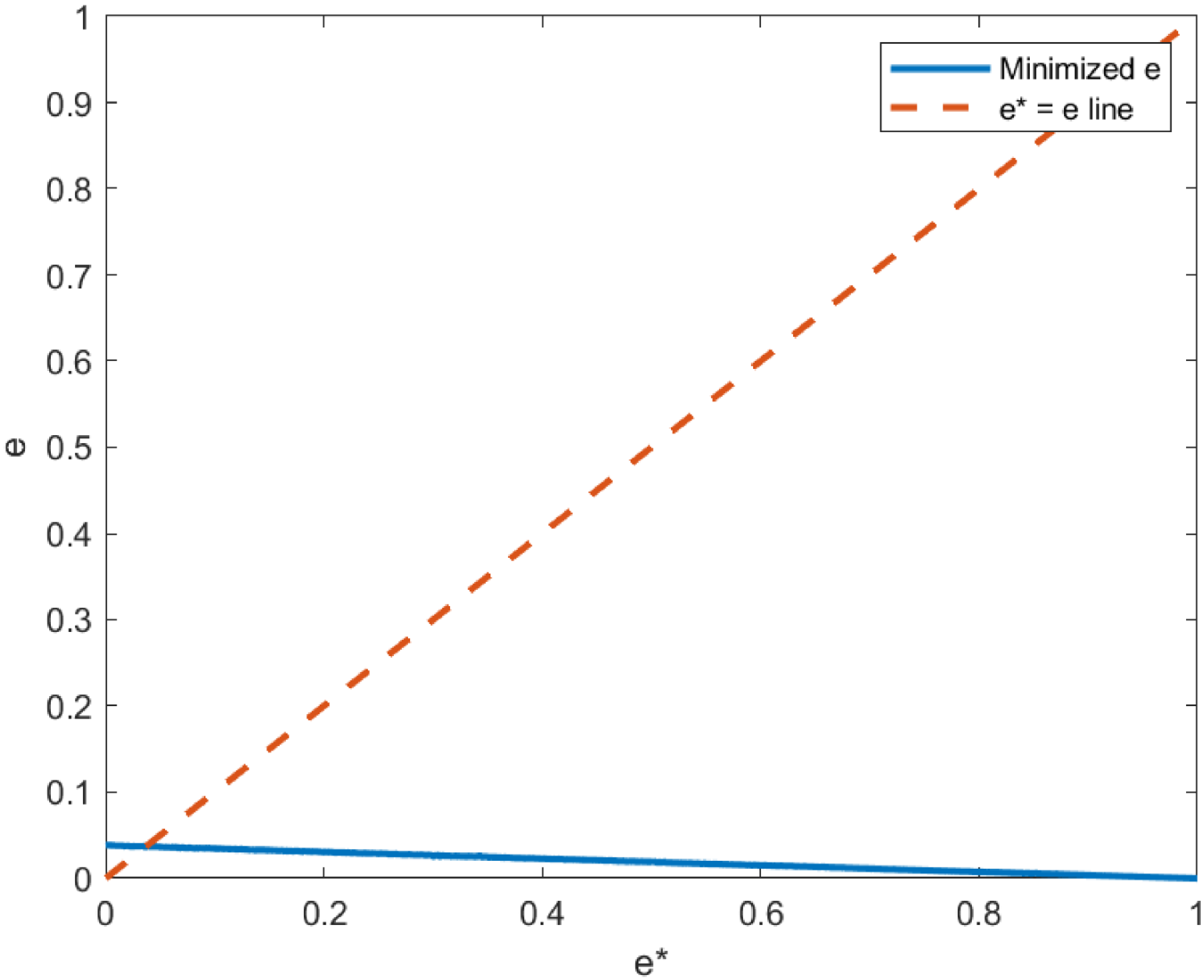
 V(e;e∗)
 e∗
 e=e∗
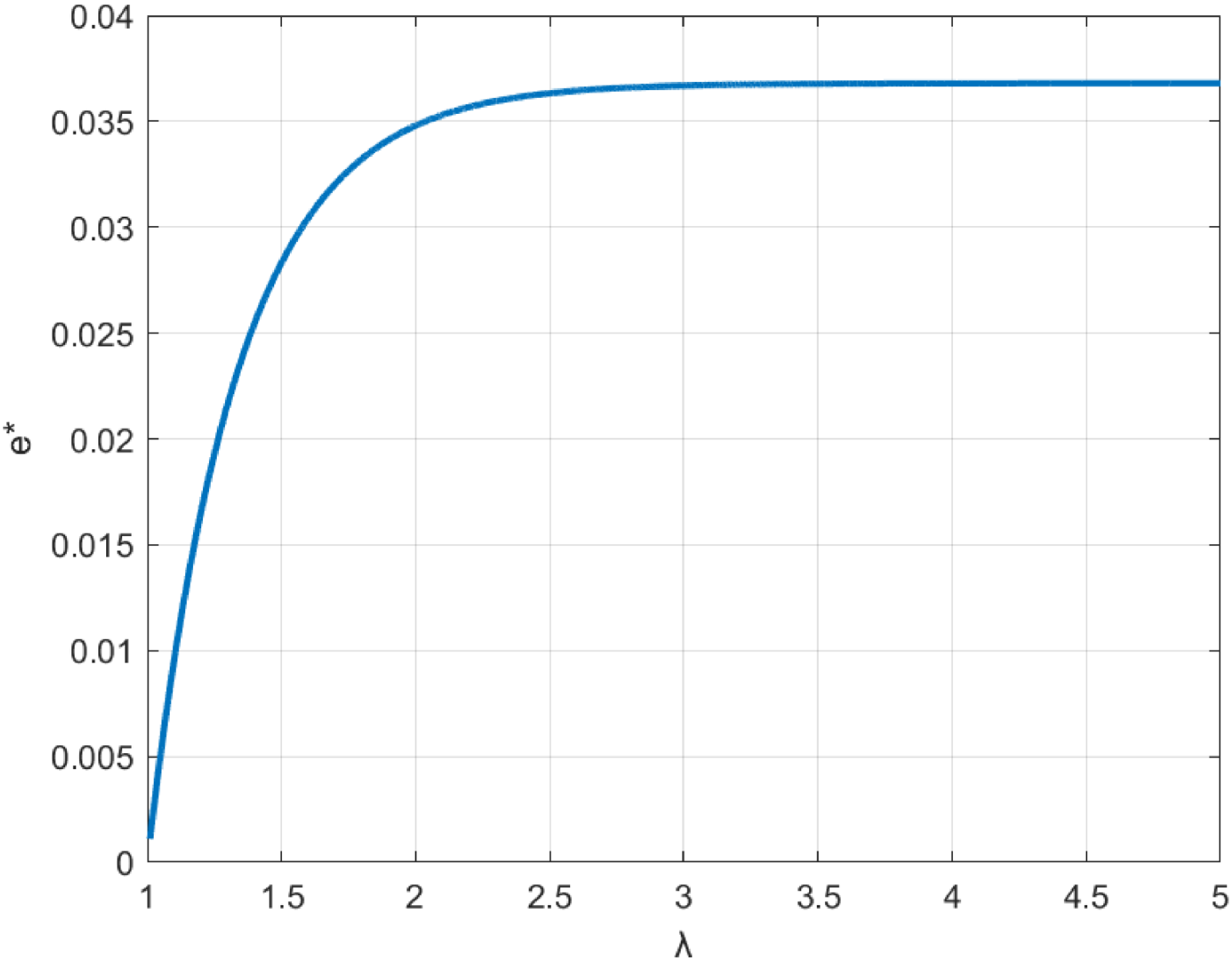
 e∗
 λ
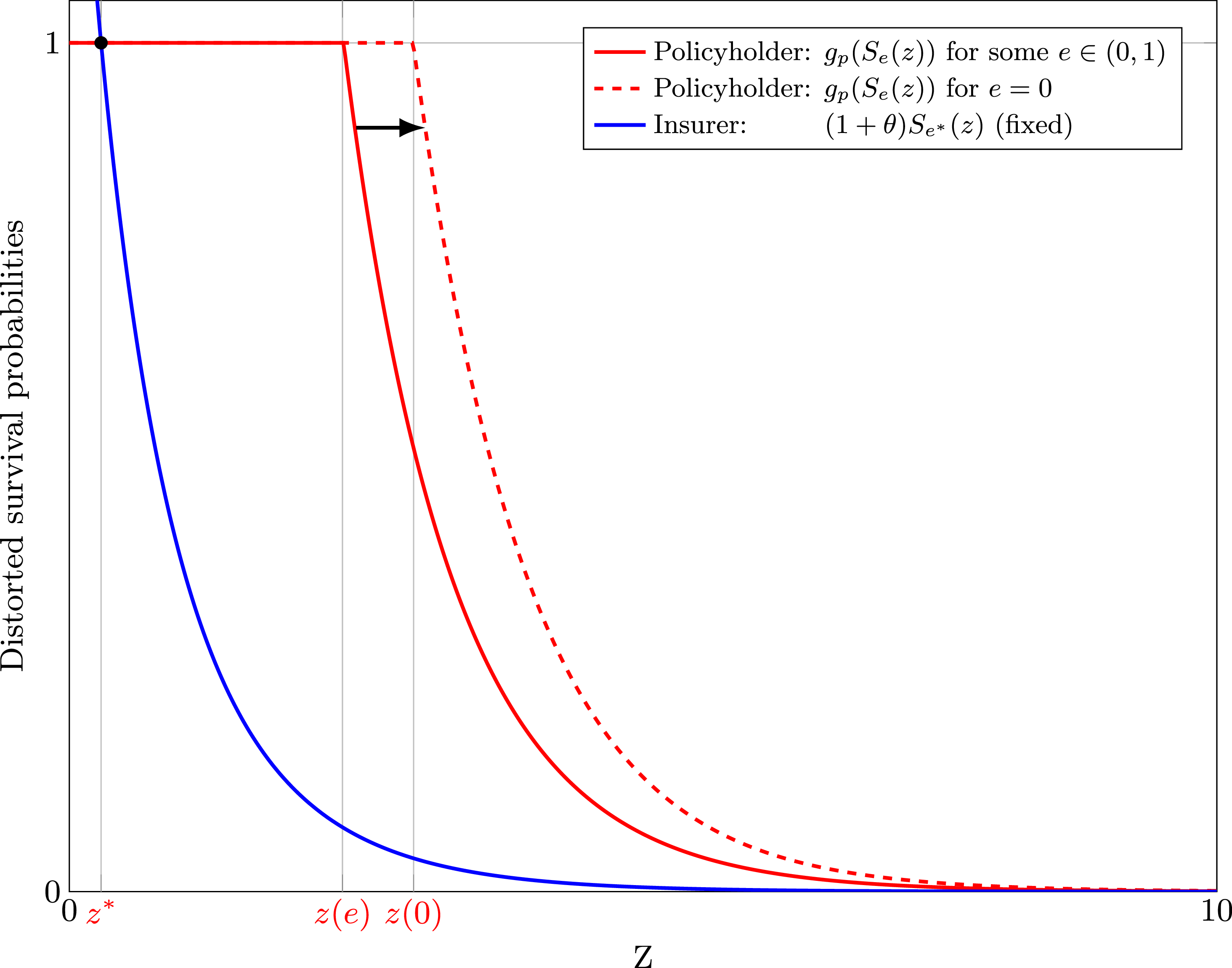
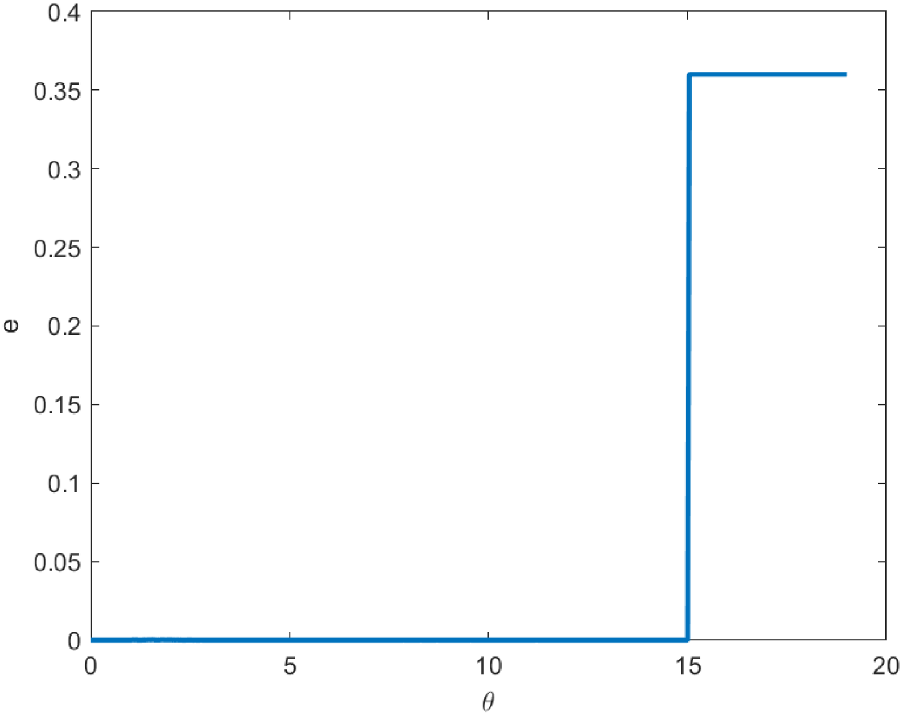
 θ
 e∗=0
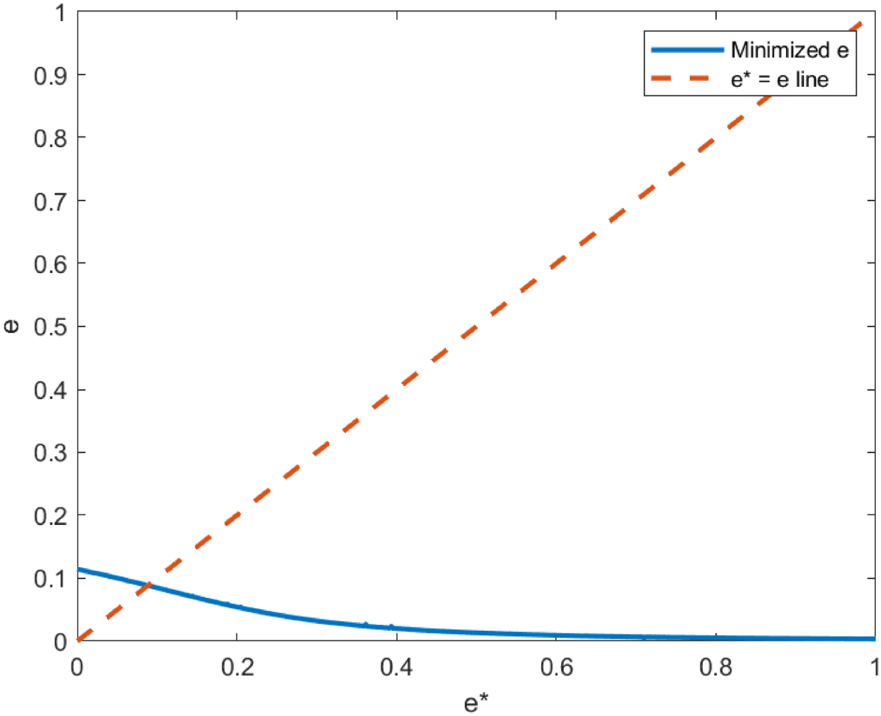
 e∗
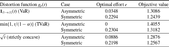
 gp

 Open access

