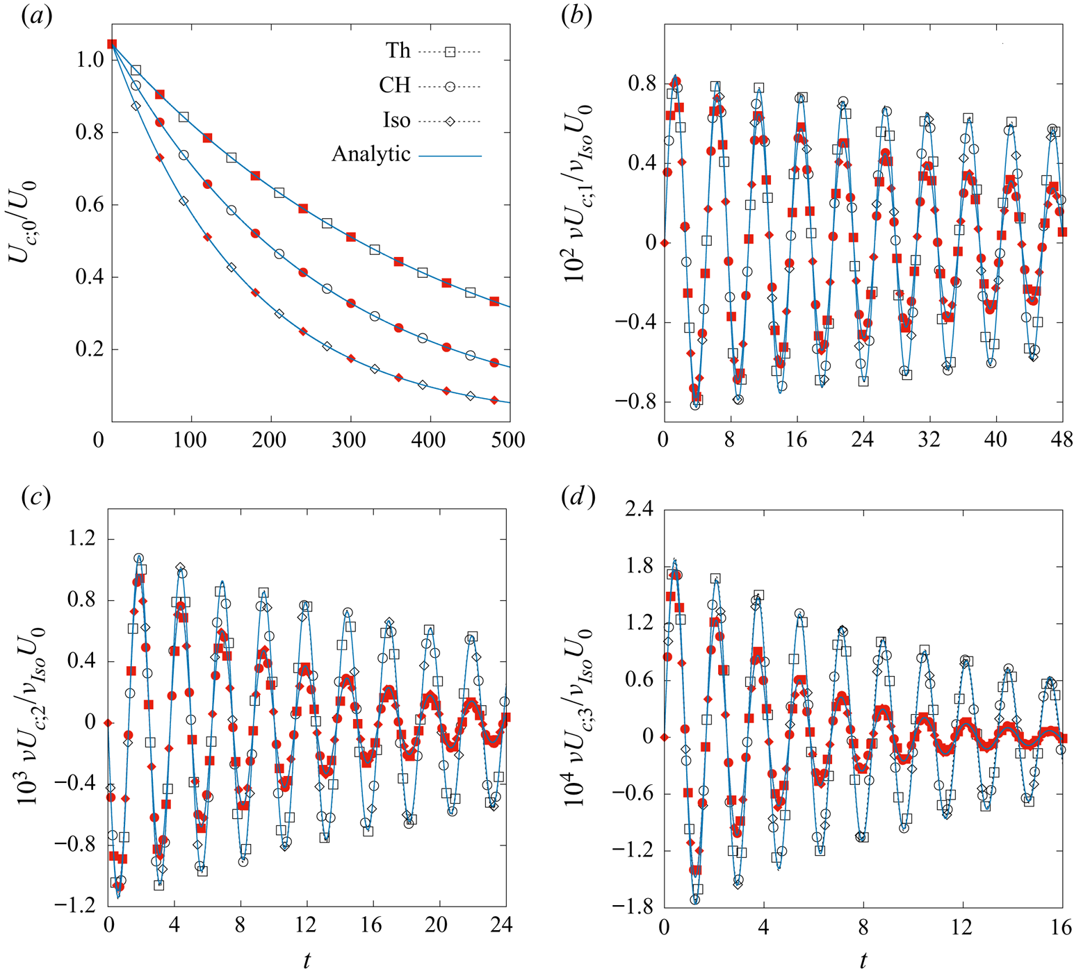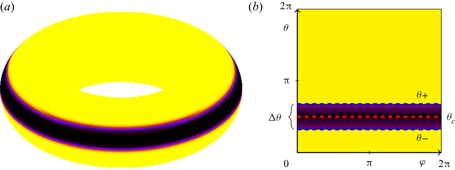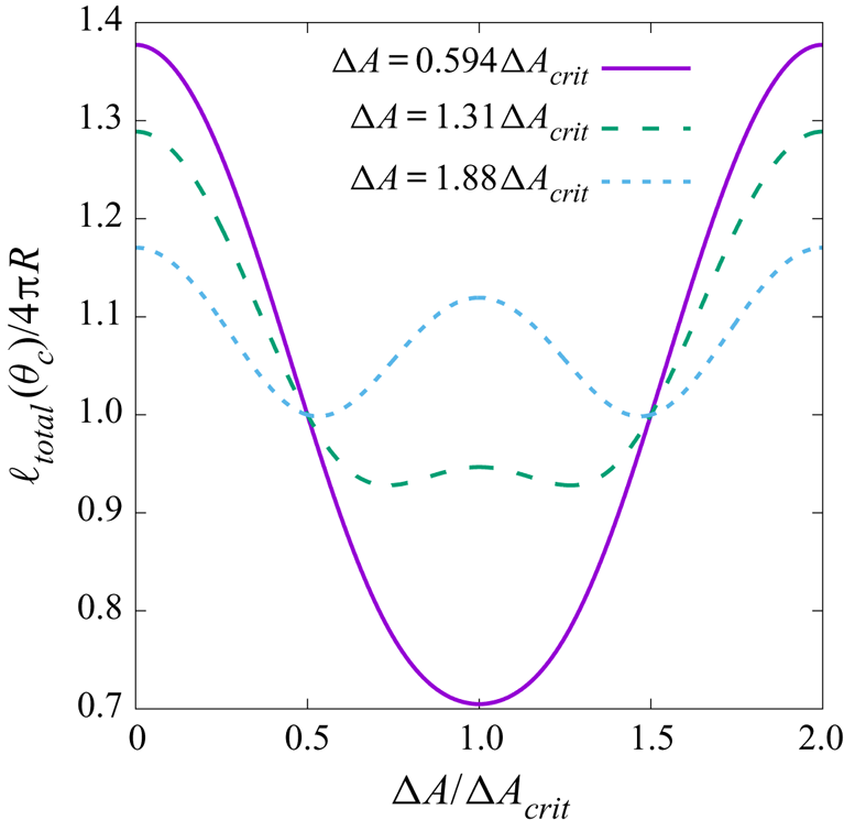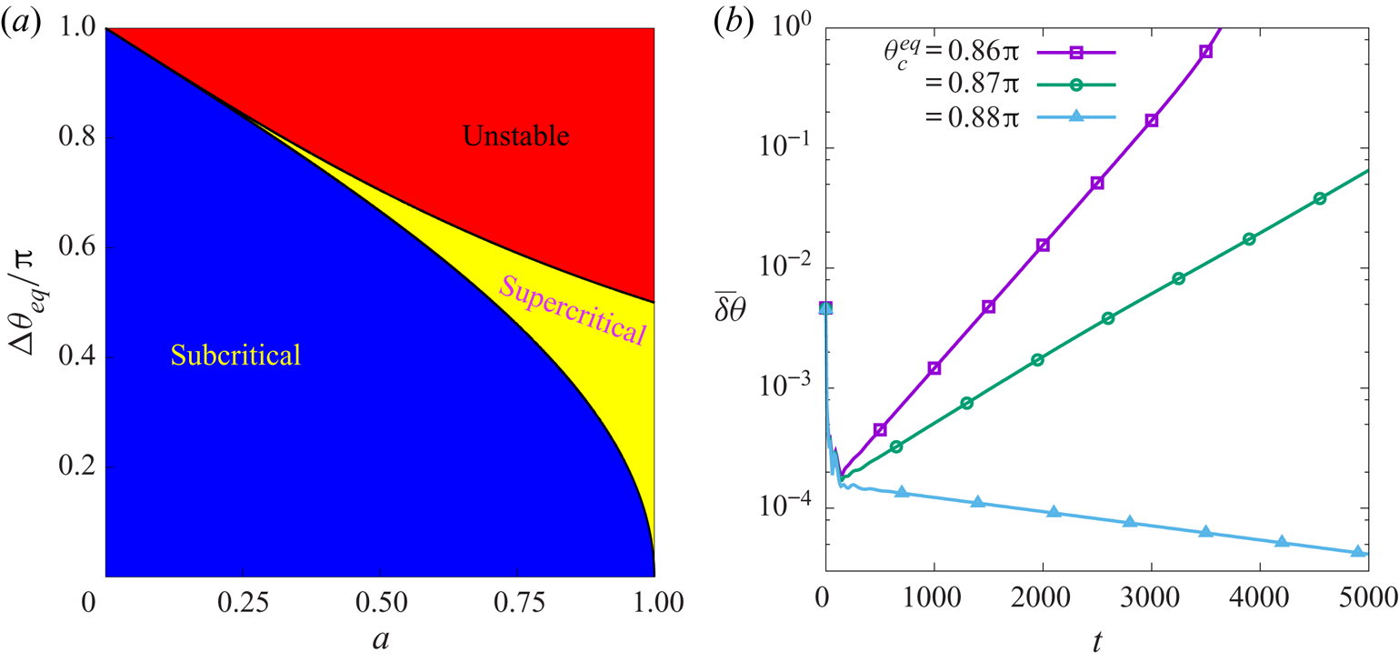


1. Introduction
In recent years there has been a growing interest in studying and understanding hydrodynamic flows on curved surfaces, supported by increasing evidence for their relevance in a wide range of problems in nature and engineering. Examples include phenomena in materials science, such as the motion of electrons in graphene (Giordanelli, Mendoza & Herrmann Reference Giordanelli, Mendoza and Herrmann2018), interface rheology in foams (Cox, Weaire & Glazier Reference Cox, Weaire and Glazier2004) and the dynamics of confined active matter (Keber et al. Reference Keber, Loiseau, Sanchez, DeCamp, Giomi, Bowick, Marchetti, Dogic and Bausch2014; Janssen, Kaiser & Löwen Reference Janssen, Kaiser and Löwen2017; Henkes, Marchetti & Sknepnek Reference Henkes, Marchetti and Sknepnek2018; Pearce et al. Reference Pearce, Ellis, Fernandez-Nieves and Giomi2019); in biophysics, such as flows on curved biomembranes (Arroyo & Desimone Reference Arroyo and Desimone2009; Henle & Levine Reference Henle and Levine2010; Al-Izzi, Sens & Turner Reference Al-Izzi, Sens and Turner2018; Fonda et al. Reference Fonda, Rinaldin, Kraft and Giomi2018) or fluid deformable surfaces (Torres-Sánchez, Millán & Arroyo Reference Torres-Sánchez, Millán and Arroyo2019; Voigt Reference Voigt2019); in fusion technology, such as plasma motion under toroidal confinement (Boozer Reference Boozer2005); and in geophysics, such as zonal flows on planets and the Sun (Sasaki, Takehiro & Yamada Reference Sasaki, Takehiro and Yamada2015).
In this work, we consider a series of axisymmetric flows on the torus geometry (i.e. flows which are homogeneous with respect to the azimuthal torus coordinate) for which analytic solutions can be derived. The torus is chosen as it represents one of the simplest geometries with non-uniform curvature. On the one hand, these flows allow us to identify novel flow phenomena arising from the presence of non-uniform curvature, which are absent on planar geometries. Importantly, our analytical calculations allow us to identify the key ingredients for observing these phenomena. On the other hand, this work can provide several non-trivial benchmark problems suitable for developing computational methods for flows on curved surfaces. To date, a number of numerical approaches have been developed to solve the fluid equations of motion on curved manifolds, including using finite-element (Dziuk & Elliott Reference Dziuk and Elliott2007, Reference Dziuk and Elliott2013), level set (Bertalmío et al. Reference Bertalmío, Cheng, Osher and Sapiro2001), phase-field (Rätz & Voigt Reference Rätz and Voigt2006), closest point (Macdonald & Ruuth Reference Macdonald and Ruuth2010) and lattice Boltzmann (Ambruş et al. Reference Ambruş, Busuioc, Wagner, Paillusson and Kusumaatmaja2019) methods. Recently, interest has been shown also for fluid systems on evolving curved manifolds both for incompressible (Koba, Liu & Giga Reference Koba, Liu and Giga2017; Nitschke, Reuther & Voigt Reference Nitschke, Reuther and Voigt2019) and compressible (Koba Reference Koba2018) fluids. However, despite the availability of these various methods, to date there is still a lack of systematic comparisons to assess and compare their accuracy and robustness. Here, we directly compare all the analytical derivations against numerical simulations obtained using a finite-difference Navier–Stokes solver.
In total we discuss five problems with increasing complexity. First, we start with the propagation of sound waves for a perfect fluid on a torus. Then, we consider viscous damping. We study shear wave damping, where the fluid velocity is in the azimuthal direction of the torus, as well as the damping of longitudinal waves, where the fluid velocity is in the poloidal direction. These three problems have been regularly studied for the planar geometry, and they are popular benchmark case studies for Navier–Stokes solvers (Sofonea & Sekerka Reference Sofonea and Sekerka2003; Rembiasz et al. Reference Rembiasz, Obergaulinger, Cerdá-Durán, Aloy and Müller2017; Sofonea et al. Reference Sofonea, Biciuşcă, Busuioc, Ambruş, Gonnella and Lamura2018; Busuioc et al. Reference Busuioc, Ambruş, Biciuşcă and Sofonea2020). Here, for their torus equivalent, we analyse the flows by deriving their distinct discrete spectrum of eigenfrequencies and corresponding basis functions. We carry out these studies for isothermal and thermal single-component fluids, as well as for multicomponent fluids described by the Cahn–Hilliard equation. Interestingly, we find that the degeneracy between odd and even modes is broken, which can be observed both in the oscillation frequencies and decay rates of those modes. Due to the non-uniform curvature, we will also show that Galilean invariance and flow periodicity, as commonly observed in the planar geometry, can be lost.
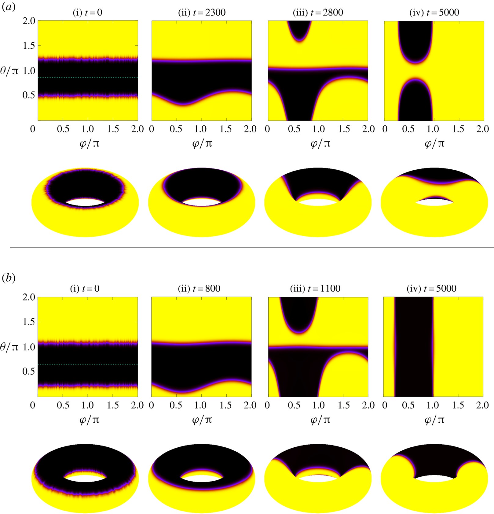
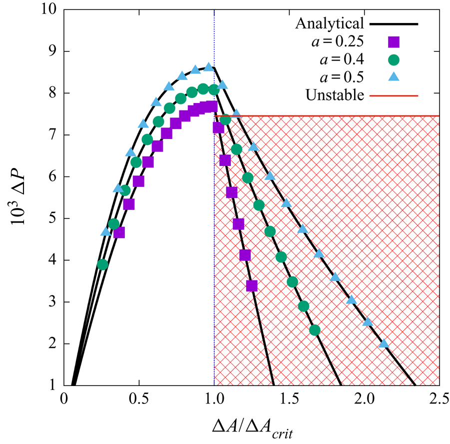
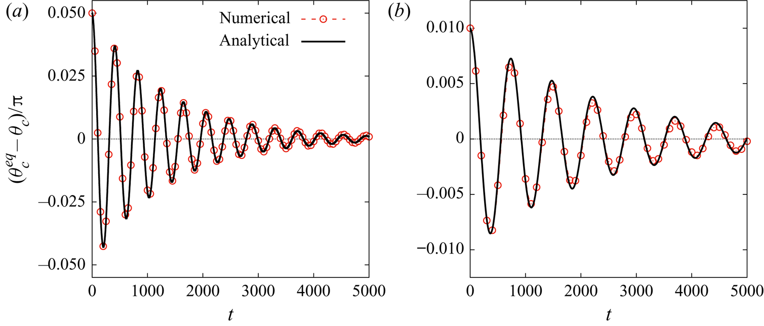
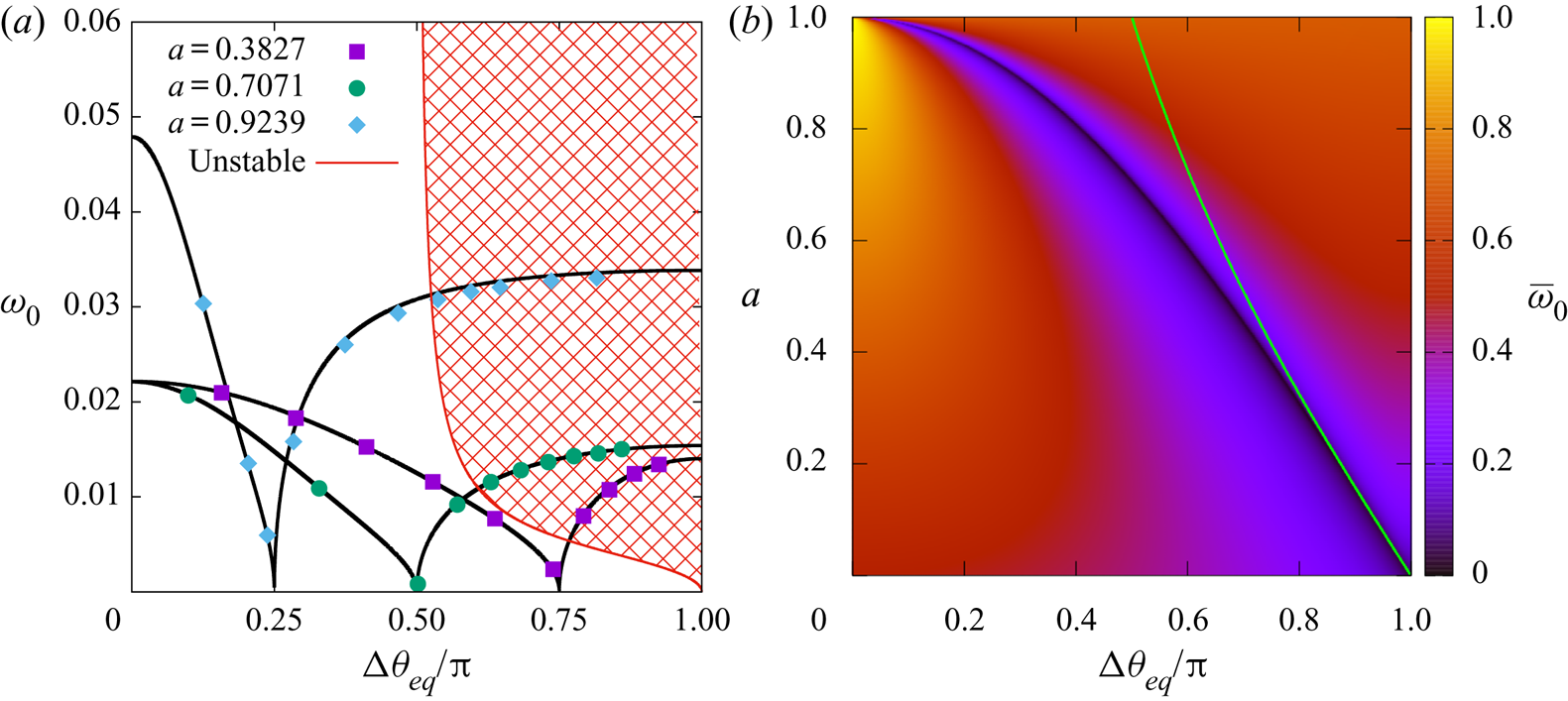
Next, we focus on an axisymmetric fluid stripe embedded on a torus. Focussing on the static configurations, the spatial symmetry is broken in the poloidal direction and we find a second-order phase transition in the location of the minimum energy configurations depending on the area of the fluid stripes. We further derive the equivalent of a Laplace pressure on a torus geometry, where additional terms are present due to the underlying curved metric. As a consequence of the phase transition, the Laplace pressure of a fluid stripe in equilibrium has a complex dependence on its area. For completeness, we also discuss other configurations, available when the axisymmetry restriction is lifted, which may have lower energy compared to the stripe configuration under certain conditions. Furthermore, we derive the regime of stability of the stripe configurations under small azimuthal perturbations. We then study the relaxation dynamics of the fluid stripes. When the Cahn–Hilliard equation is coupled with hydrodynamics, we find an underdamped oscillatory motion for the stripe dynamics. We derive the oscillation frequency and the exponential decay rate. The case in the absence of hydrodynamics, where the stripes simply relax exponentially to their equilibrium position, is discussed in § SM:2.4 of the supplementary material available at https://doi.org/10.1017/jfm.2020.440.
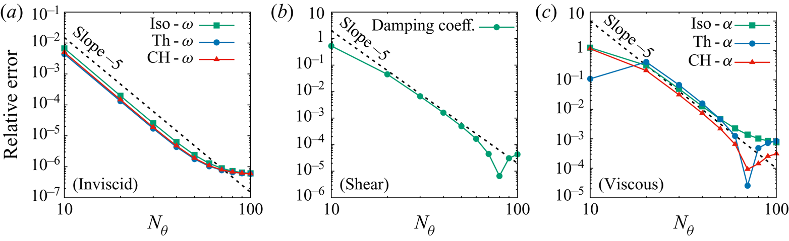
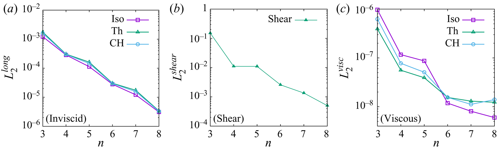
The paper is structured as follows. Section 2 describes the hydrodynamic equations for flows on general curved surfaces, which are then specialised to the case of axisymmetric flows on the torus geometry. The five axisymmetric flow problems are introduced and presented in §§ 3–7. Taken together, our series of axisymmetric flows cover single- and multi-component flows, static and dynamic aspects, instabilities under small perturbations, perfect and viscous fluids, isothermal and thermal cases and motion in the azimuthal and poloidal directions of the torus. A summary of the work and concluding remarks are finally presented in § 8. The paper also includes two appendices. Appendix A presents a convergence order analysis of the solver employed in this paper with respect to the first three benchmark tests, discussed in §§ 3–5. Appendix B discusses the perturbative procedure that we use to obtain the mode solutions necessary for the spatial part of the linearised hydrodynamic equations, which are employed in the main text.
The supplementary material (SM) contains three sections. Section SM:1 provides details on the implementation of our numerical scheme. Section SM:2 contains mathematical complements for the analysis of the Cahn–Hilliard model on the torus geometry. Finally, § SM:3 applies the procedure described in appendix B to derive expansions of the mode functions and related quantities up to ninth order with respect to the torus aspect ratio,  $0 < a = r / R < 1$. These expansions are available for download as gnuplot files (funcs-inv.gpl and funcs-shear.gpl) and Mathematica notebooks (funcs_inv.nb and funcs_shear.nb) in the supplementary material. In addition, two animations of the development of the instability of fluid stripes due to azimuthal perturbations, discussed in § 6.2, are also provided in the supplementary material.
2. Hydrodynamics on curved surfaces
Over the past decades, there have been several attempts to formulate the hydrodynamic equations on curved surfaces (Serrin Reference Serrin, Flügge and Truesdell1959; Marsden & Hughes Reference Marsden and Hughes1994; Taylor Reference Taylor2011). In this paper, we take the strategy of first writing the fluid equations with respect to curvilinear coordinates in covariant form. Employing the orthonormal vielbein vector field  $\{\boldsymbol {e}_{\hat {\alpha }}, \alpha = 1, 2, 3\}$, we then take the first two vectors,
 $\boldsymbol {e}_{{\hat {\imath }}}$ (
 $i = 1, 2$) to be tangent to the manifold and enforce that no dynamics occurs along the third vector,
 $\boldsymbol {e}_{\hat {3}}$. This approach allows the fundamental conservation equations for mass, momentum and energy for fluids on a curved surface to be written in covariant form as follows:
 \begin{gather} \frac{\textrm{D}\rho}{\textrm{D}t} + \rho \nabla_{\hat{\imath}} u^{\hat{\imath}} = 0, \end{gather}
 \begin{gather}\rho \frac{\textrm{D}u^{\hat{\imath}}}{\textrm{D}t} + \nabla_{{\hat{\jmath}}} \boldsymbol{\mathsf{T}}^{{\hat{\imath}}{\hat{\jmath}}} = \rho f^{\hat{\imath}}, \end{gather}
 \begin{gather}\rho \frac{\textrm{D}e}{\textrm{D}t} + \boldsymbol{\mathsf{T}}^{{\hat{\imath}}{\hat{\jmath}}} \nabla_{\hat{\imath}} u_{\hat{\jmath}} = - \nabla_{\hat{\imath}} q^{\hat{\imath}}, \end{gather}
where  $1 \le i,j \le 2$ cover the tensor components along the directions which are tangent to the surface. In the above,
 $\rho$ is the fluid mass density,
 $\boldsymbol {u} = u^{\hat {\imath }} \boldsymbol {e}_{\hat {\imath }}$ is the fluid velocity,
 $\nabla _{\hat {\imath }}$ is the covariant derivative,
 $\textrm {D}/\textrm {D}t = \partial _t + u^{\hat {\jmath }} \nabla _{\hat {\jmath }}$ is the material (convective) derivative,
 $\boldsymbol{\mathsf{T}}^{{\hat {\imath }}{\hat {\jmath }}}$ is the pressure tensor,
 $f^{\hat {\imath }}$ is the external force per unit mass (which we neglect for the remainder of this paper),
 $e = c_v T$ is the internal energy per unit mass,
 $c_v$ is the specific heat capacity,
 $T$ is the fluid temperature and
 $q^{\hat {\imath }}$ is the heat flux. The set of relations (2.1a)–(2.1c) are compatible with those derived from kinetic theory in curvilinear coordinates (Busuioc & Ambruş Reference Busuioc and Ambruş2019) or on curved manifolds (Ambruş et al. Reference Ambruş, Busuioc, Wagner, Paillusson and Kusumaatmaja2019). Furthermore, the computation of the divergence of the stress tensor in a covariant way ensures the compatibility with the approaches currently taken in the literature (Arroyo & Desimone Reference Arroyo and Desimone2009; Taylor Reference Taylor2011; Nitschke, Reuther & Voigt Reference Nitschke, Reuther, Voigt, Bothe and Reusken2017; Gross & Atzberger Reference Gross and Atzberger2018).
The hydrodynamic equations, (2.1), are not closed unless the pressure tensor  $\boldsymbol{\mathsf{T}}^{{\hat {\imath }}{\hat {\jmath }}}$ and heat flux
 $q^{{\hat {\imath }}}$ are known. The specific models employed in this paper for these quantities are discussed below in §§ 2.1 and 2.2, respectively. After briefly introducing the relevant differential operators in § 2.3, we explicitly write the equations of motion for axisymmetric flows on the torus geometry in § 2.4.
2.1. Models for the pressure tensor
We restrict our analysis to the case of Newtonian fluids, for which the pressure tensor can be decomposed as
 \begin{equation} \boldsymbol{\mathsf{T}}^{{\hat{\imath}}{\hat{\jmath}}} = {\textit{P}}_{b} \delta^{{\hat{\imath}}{\hat{\jmath}}}+ \boldsymbol{\mathsf{P}}_{\kappa}^{{\hat{\imath}}{\hat{\jmath}}} - \tau^{{\hat{\imath}}{\hat{\jmath}}}. \end{equation}
The dissipative part 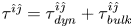 $\tau ^{{\hat {\imath }}{\hat {\jmath }}} = \tau ^{{\hat {\imath }}{\hat {\jmath }}}_{\mathit {dyn}} + \tau ^{{\hat {\imath }}{\hat {\jmath }}}_{\mathit {bulk}}$ of the pressure tensor for a two-dimensional Newtonian fluid reads
 \begin{equation}\tau^{{\hat{\imath}}{\hat{\jmath}}}_{\mathit{dyn}} = \eta\left(\nabla^{\hat{\imath}} u^{\hat{\jmath}} + \nabla^{\hat{\jmath}} u^{\hat{\imath}} - \delta^{{\hat{\imath}}{\hat{\jmath}}} \nabla_{\hat{k}} u^{\hat{k}}\right), \quad \tau^{{\hat{\imath}}{\hat{\jmath}}}_{\mathit{bulk}} = \eta_v \delta^{{\hat{\imath}}{\hat{\jmath}}} \nabla_{\hat{k}} u^{\hat{k}}, \end{equation}
where  $\eta$ and
 $\eta _v$ are the dynamic and bulk (volumetric) viscosity coefficients, respectively. For the applications considered in this work, the dependence of the transport coefficients on the flow properties is not important. Hence, we adopt the usual model in which the kinematic viscosities
 $\nu$ and
 $\nu _v$ are constant, such that
 $\eta$ and
 $\eta _v$ are computed using
 \begin{equation}\eta = \nu \rho,\quad \eta_v = \nu_v \rho. \end{equation}
For the first two terms in (2.2),  $P_{b}$ is the isotropic bulk pressure and
 $\boldsymbol{\mathsf{P}}_{\kappa }^{{\hat {\imath }}{\hat {\jmath }}}$ is responsible for the surface tension, which is relevant in the case of multicomponent systems. For ideal single-component fluids, the bulk pressure is the ideal gas pressure and the surface tension part vanishes
 \begin{equation} P_{b} = P_{i} = \frac{\rho k_B T}{m}, \quad \boldsymbol{\mathsf{P}}^{{\hat{\imath}}{\hat{\jmath}}}_{\kappa} = 0, \end{equation}
where  $m$ is the average particle mass. In this paper, we always use units such that
 $m=1$.
For multicomponent flows, we consider a binary mixture of fluids  ${\mathcal {A}}$ and
 ${\mathcal {B}}$, characterised by an order parameter
 $\phi$, such that
 $\phi = 1$ corresponds to a bulk
 ${\mathcal {A}}$ fluid and
 $\phi = -1$ to a bulk
 ${\mathcal {B}}$ fluid. The coexistence of these two bulk fluids can be realised by using a simple form for the Helmholtz free energy
 $\Psi$
 \begin{equation} \Psi = \int_V \textrm{d} V(\psi_{b} + \psi_{g}), \end{equation}
where the bulk  $\psi _{b}$ and the gradient
 $\psi _{g}$ free energy densities are (Briant & Yeomans Reference Briant and Yeomans2004; Krüger et al. Reference Krüger, Kusumaatmaja, Kuzmin, Shardt, Silva and Viggen2017)
 \begin{equation}\psi_{b} = \frac{A}{4} (1-\phi^2)^2, \quad \psi_{g} = \frac{\kappa}{2} (\nabla \phi)^2. \end{equation}
Here,  $A$ and
 $\kappa$ are free parameters, which are related to the interface width
 $\xi$ and surface tension
 $\sigma$ through
 \begin{equation}\xi = \sqrt{\frac{\kappa}{A}}, \quad \sigma = \sqrt{\frac{8 \kappa A}{9}}. \end{equation}
For simplicity, we consider the case when  $A$ and
 $\kappa$ have constant values throughout the fluid. The chemical potential can be derived by taking the functional derivative of the free energy with respect to the order parameter, giving
 \begin{equation} \mu = \frac{\delta \Psi}{\delta \phi} = \mu_{b} + \mu_{g}, \quad \mu_{b} = -A\phi(1- \phi^2), \quad \mu_{g} = - \kappa {\rm \Delta} \phi. \end{equation}
The additional contributions to the pressure tensor arising from this free energy model can be found by imposing
 \begin{equation} \nabla_{\hat{\jmath}} [P_{CH} \delta^{{\hat{\imath}}{\hat{\jmath}}} + \boldsymbol{\mathsf{P}}_{{CH}; \kappa}^{{\hat{\imath}}{\hat{\jmath}}}] = \phi \nabla^{\hat{\imath}} \mu, \end{equation}
which leads to
 \begin{equation} \left.\begin{array}{c@{}} P_{b} = P_{i} + P_{CH} = \dfrac{\rho k_B T}{m} -A \left(\dfrac{\phi^2}{2} - \dfrac{3\phi^4}{4}\right), \\ \boldsymbol{\mathsf{P}}^{{\hat{\imath}}{\hat{\jmath}}}_{\kappa} = \boldsymbol{\mathsf{P}}^{{\hat{\imath}}{\hat{\jmath}}}_{{CH}; \kappa} = \kappa \nabla^{\hat{\imath}} \phi \nabla^{\hat{\jmath}} \phi - \kappa \delta^{{\hat{\imath}}{\hat{\jmath}}} \left[ \phi {\rm \Delta} \phi +\dfrac{1}{2} (\nabla \phi)^2\right]. \end{array}\right\} \end{equation}
For multicomponent flows, in addition to the hydrodynamic equations in (2.1), another equation of motion is needed to capture the evolution of the order parameter  $\phi$. Here, it is governed by the Cahn–Hilliard equation
 \begin{equation} \frac{{\rm D}\phi}{{\rm D}t} + \phi \nabla_{\hat{\imath}} u^{\hat{\imath}} = \nabla_{\hat{\imath}} (M \nabla^{\hat{\imath}} \mu), \end{equation}
where  $M$ is the mobility parameter,
 ${\rm D}/{\rm D}t = \partial _t + u^{\hat {\imath }} \nabla _{\hat {\imath }}$ is the material derivative and the fluid velocity
 $\boldsymbol {u}$ is a solution of the hydrodynamic equations (2.1). For simplicity, we assume that
 $M$ takes a constant value throughout the fluid.
2.2. Model for the heat flux
We consider fluids for which the heat flux is given via Fourier's law
 \begin{equation} q^{{\hat{\imath}}} = - k \nabla^{\hat{\imath}} T. \end{equation}
The heat conductivity  $k$ is related to the dynamic viscosity through the Prandtl number
 $Pr$
 \begin{equation} Pr = c_p \frac{\eta}{k} =c_v \frac{\gamma \eta}{k}, \end{equation}
where  $c_p$ is the specific heat at constant pressure and
 $\gamma$ is the adiabatic index. For definiteness, we assume that
 $Pr$ is a constant number in this work.
When considering isothermal flows, the temperature is assumed to remain constant and the heat flux vanishes
 \begin{equation} T = T_{\mathit{Iso}} = \textrm{const}, \quad q^{\hat{\imath}}_{\mathit{Iso}} = 0. \end{equation}
In this case, the energy equation is no longer taken into consideration.
2.3. Differential operators on the torus geometry
In this subsection we provide a brief introduction to the differential geometry approach we have used to analyse the fluid flows. For concreteness, we consider the parametrisation of a torus of outer radius  $R$ and inner radius
 $r$ using the coordinates
 $q^i \in \{\varphi , \theta \}$ (
 $i$ represents a coordinate index) as follows:
 \begin{equation} \left.\begin{array}{c@{}} x = (R + r \cos \theta) \cos \varphi,\\ y = (R + r \cos \theta) \sin \varphi,\\ z = r \sin \theta. \end{array}\right\} \end{equation}
Here,  $\varphi$ and
 $\theta$ are the azimuthal and the poloidal angles, respectively, and the system is periodic with respect to both angles with period of
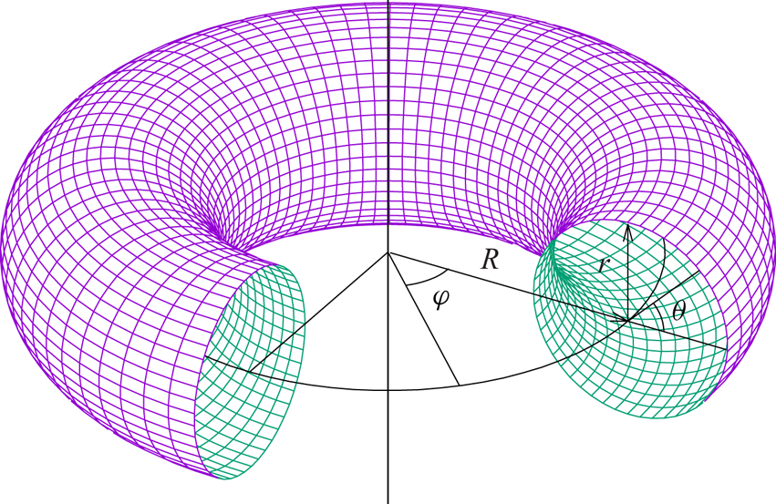
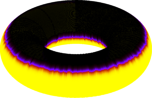
 $2{\rm \pi}$. Figure 1 depicts the coordinates and the equidistant spatial discretisation in
 $\varphi$ and
 $\theta$.
Spatial discretisation of the torus geometry.

The line element on the torus can be written with respect to  $\theta$ and
 $\varphi$ as follows:
 \begin{equation} \textrm{d}s^2 = (R + r \cos\theta)^2 \,\textrm{d}\varphi^2 + r^2 \,\textrm{d}\theta^2. \end{equation}
The metric tensor associated with the above line element has the following non-vanishing components:
 \begin{equation} \boldsymbol{\mathsf{g}}_{\varphi\varphi} = (R + r \cos\theta)^2, \quad \boldsymbol{\mathsf{g}}_{\theta\theta} = r^2. \end{equation}
Similar to the approach taken by other authors (Nitschke, Voigt & Wensch Reference Olver, Lozier, Boisvert and ClarkReference Nitschke, Voigt and Wensch2012; Reuther & Voigt Reference Reuther and Voigt2018), it is convenient to introduce the vielbein vector frame  $\{\boldsymbol {e}_{{\hat {\varphi }}}, \boldsymbol {e}_{{\hat {\theta }}}\}$, where
 $\boldsymbol {e}_{\hat {\imath }} = e_{\hat {\imath }}^i \boldsymbol {\partial }_i$ is the notation for a vector tangent to the surface. The components
 $e_{\hat {\imath }}^i$ satisfy
 \begin{equation} \boldsymbol{\mathsf{g}}_{ij} e^i_{\hat{\imath}} e^{\, j}_{\hat{\jmath}} = \delta_{{\hat{\imath}}{\hat{\jmath}}}. \end{equation}
The natural choice for the vielbein on the torus geometry is
 \begin{equation} \boldsymbol{e}_{\hat{\varphi}} = \frac{\boldsymbol{\partial}_\varphi}{R(1 +a \cos\theta)}, \quad \boldsymbol{e}_{\hat{\theta}} = \frac{\boldsymbol{\partial}_\theta}{r}, \end{equation}
where the following notation was introduced for future convenience:
 \begin{equation} a = \frac{r}{R}. \end{equation}
The corresponding vielbein co-frame, comprised of the one-forms  $\boldsymbol {\omega }^{\hat {\imath }} = \omega ^{{\hat {\imath }}}_i \boldsymbol {dq}^i$, is given by
 \begin{equation} \boldsymbol{\omega}^{\hat{\varphi}} = R(1 + a\cos\theta) \boldsymbol{d\varphi}, \quad \boldsymbol{\omega}^{\hat{\theta}} = r \boldsymbol{d\theta}, \end{equation}
such that
 \begin{equation} \omega^{\hat{\imath}}_i e_{{\hat{\jmath}}}^i = \delta^{{\hat{\imath}}}{}_{\hat{\jmath}}, \quad \delta_{{\hat{\imath}}{\hat{\jmath}}} \omega^{\hat{\imath}}_i \omega^{\hat{\jmath}}_j = g_{ij}. \end{equation}
The algebraic rules to compute the terms appearing in (2.1) are described below. The gradient 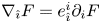 $\nabla _{\hat {\imath }} F = e_{\hat {\imath }}^i \partial _i F$ of a scalar function
 $F$ has the following components:
 \begin{equation} \nabla_{\hat{\varphi}} F = \frac{\partial_\varphi F}{R(1 + a\cos\theta)}, \quad \nabla_{\hat{\theta}} F = \frac{1}{r} \partial_\theta F. \end{equation}
For a vector field  $A^{\hat {\imath }}$, the covariant derivative is
 \begin{equation} \nabla_{\hat{\jmath}} A^{\hat{\imath}} = e_{\hat{\jmath}}^{\, j} \partial_j A^{{\hat{\imath}}} + \Gamma^{\hat{\imath}}{}_{{\hat{k}}{\hat{\jmath}}} A^{\hat{k}}, \end{equation}
and when the vector index is lowered, it becomes
 \begin{equation} \nabla_{\hat{\jmath}} A_{\hat{\imath}} = e_{\hat{\jmath}}^{\,j} \partial_j A_{\hat{\imath}} - \Gamma^{\hat{k}}{}_{{\hat{\imath}}{\hat{\jmath}}} A_{\hat{k}}. \end{equation}
For the computation of the covariant derivatives, the connection coefficients 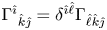 $\Gamma ^{\hat {\imath }}{}_{{\hat {k}}{\hat {\jmath }}} = \delta ^{{\hat {\imath }}{\hat {\ell }}} \Gamma _{{\hat {\ell }}{\hat {k}}{\hat {\jmath }}}$ are defined as
 \begin{equation} \Gamma_{{\hat{\ell}}{\hat{k}}{\hat{\jmath}}} = \tfrac{1}{2}(c_{{\hat{\ell}}{\hat{k}}{\hat{\jmath}}} + c_{{\hat{\ell}}{\hat{\jmath}}{\hat{k}}} - c_{{\hat{k}}{\hat{\jmath}}{\hat{\ell}}}), \end{equation}
with the Cartan coefficients 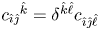 $c_{{\hat {\imath }}{\hat {\jmath }}}{}^{{\hat {k}}} = \delta ^{{\hat {k}}{\hat {\ell }}} c_{{\hat {\imath }}{\hat {\jmath }}{\hat {\ell }}}$ to be computed from the commutator of the vectors of the vielbein field
 \begin{equation} [\boldsymbol{e}_{{\hat{\imath}}}, \boldsymbol{e}_{{\hat{\jmath}}}] = c_{{\hat{\imath}}{\hat{\jmath}}}{}^{{\hat{k}}} \boldsymbol{e}_{\hat{k}}, \end{equation}
where the components of the commutator are  $([\boldsymbol {e}_{{\hat {\imath }}}, \boldsymbol {e}_{{\hat {\jmath }}}])^d = e_{\hat {\imath }}^k \partial _k e_{\hat {\jmath }}^d - e_{\hat {\jmath }}^k \partial _k e_{\hat {\imath }}^d$. We can also invert the above relation to get
 \begin{equation} c_{{\hat{\imath}}{\hat{\jmath}}}{}^{{\hat{k}}} = \langle [\boldsymbol{e}_{{\hat{\imath}}}, \boldsymbol{e}_{{\hat{\jmath}}}], \boldsymbol{\omega}^{{\hat{k}}}\rangle = (e_{\hat{\imath}}^d e_{\hat{\jmath}}^k - e_{\hat{\jmath}}^d e_{\hat{\imath}}^k) \partial_k \omega_d^{{\hat{k}}}, \end{equation}
where 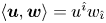 $\langle \boldsymbol {u}, \boldsymbol {w}\rangle = u^{\hat {\imath }} w_{\hat {\imath }}$ is the inner product between a vector field
 $\boldsymbol {u} = u^{\hat {\imath }} \boldsymbol {e}_{\hat {\imath }}$ and a one-form
 $\boldsymbol {w} = w_{\hat {\imath }} \boldsymbol {\omega }^{\hat {\imath }}$.
Let us now apply these definitions for the case of a torus. The commutator of the vielbein vectors  $\boldsymbol {e}_{\hat {\theta }}$ and
 $\boldsymbol {e}_{\hat {\varphi }}$ is
 \begin{equation} [\boldsymbol{e}_{\hat{\theta}}, \boldsymbol{e}_{\hat{\varphi}}] = -[\boldsymbol{e}_{\hat{\varphi}}, \boldsymbol{e}_{\hat{\theta}}] = \frac{\sin\theta}{R(1 + a\cos\theta)} \boldsymbol{e}_{\hat{\varphi}}. \end{equation}
Substituting these relations into the definition of the Cartan coefficients, we find that the only non-vanishing Cartan coefficients are
 \begin{equation} c_{{\hat{\theta}}{\hat{\varphi}}}{}^{{\hat{\varphi}}} = -c_{{\hat{\varphi}}{\hat{\theta}}}{}^{{\hat{\varphi}}} = \frac{\sin\theta}{R(1 + a\cos\theta)}, \end{equation}
and the ensuing connection coefficients read
 \begin{equation} \Gamma_{{\hat{\theta}}{\hat{\varphi}}{\hat{\varphi}}} = -\Gamma_{{\hat{\varphi}}{\hat{\theta}}{\hat{\varphi}}} = \frac{\sin\theta}{R(1 + a\cos\theta)}.\end{equation}
Another important operator is the divergence of a vector field, where the following relation applies:
 \begin{equation} \nabla_{\hat{\imath}} A^{\hat{\imath}} = \frac{1}{\sqrt{g}} \partial_i (\sqrt{g} e_{\hat{\imath}}^i A^{{\hat{\imath}}}) = \frac{\partial_\varphi A^{{\hat{\varphi}}}}{R(1 + a \cos\theta)} + \frac{\partial_\theta[A^{{\hat{\theta}}}(1 + a \cos\theta)]} {r(1 + a \cos\theta)}. \end{equation}
For the special case where  $A^{\hat {\imath }} = \nabla ^{\hat {\imath }} F$ is the gradient of a scalar function, the following relation may be employed:
 \begin{equation} {\rm \Delta} F = \nabla_{\hat{\imath}} \nabla^{\hat{\imath}} F = \frac{1}{\sqrt{g}} \partial_i (\sqrt{g} g^{ij} \partial_j F) = \frac{\partial_\varphi^2 A}{R^2 (1 + a \cos\theta)^2} + \frac{\partial_\theta[(1 + a \cos\theta) \partial_\theta F]} {r^2(1 + a \cos\theta)}.\end{equation}
Finally, the action of the covariant derivative on a tensor with two indices can be computed using
 \begin{equation} \nabla_{\hat{\imath}} \boldsymbol{\mathsf{M}}^{{\hat{\jmath}}{\hat{k}}} = e_{\hat{\imath}}^i \partial_i \boldsymbol{\mathsf{M}}^{{\hat{\jmath}}{\hat{k}}} + \Gamma^{{\hat{\jmath}}}{}_{{\hat{\ell}}{\hat{\imath}}} \boldsymbol{\mathsf{M}}^{{\hat{\ell}}{\hat{k}}} + \Gamma^{{\hat{k}}}{}_{{\hat{\ell}}{\hat{\imath}}} \boldsymbol{\mathsf{M}}^{{\hat{\jmath}}{\hat{\ell}}}. \end{equation}
2.4. Equations of motion for axisymmetric flows on the torus geometry
In this paper, we focus on axisymmetric flows, for which all fluid quantities are independent of the  $\varphi$ angular coordinate. In this case, the continuity equation (2.1a) becomes
 \begin{equation} \frac{\partial \rho}{\partial t} + \frac{\partial_\theta [\rho u^{\hat{\theta}}(1 + a \cos\theta)]} {r(1 + a \cos\theta)} = 0.\end{equation}
To derive the Cauchy equation (2.1b), let us first consider the viscous contributions to the pressure tensor. Taking the covariant derivatives in (2.3), the following expressions are obtained for the components of  $\tau _{\mathit {dyn}}^{{\hat {\imath }}{\hat {\jmath }}}$:
 \begin{equation} \left.\begin{array}{c@{}} \tau^{{\hat{\theta}}{\hat{\theta}}}_{\mathit{dyn}} = -\tau_{\mathit{dyn}}^{{\hat{\varphi}}{\hat{\varphi}}} = \dfrac{\eta}{r} (1 + a \cos\theta) \dfrac{\partial}{\partial\theta} \left( \dfrac{u^{{\hat{\theta}}}}{1 + a \cos\theta}\right), \\ \tau_{\mathit{dyn}}^{{\hat{\theta}}{\hat{\varphi}}} = \tau_{\mathit{dyn}}^{{\hat{\varphi}}{\hat{\theta}}} = \dfrac{\eta}{r} (1 + a \cos\theta) \dfrac{\partial}{\partial\theta} \left( \dfrac{u^{{\hat{\varphi}}}}{1 + a \cos\theta}\right), \end{array}\right \} \end{equation}
while the volumetric parts are
 \begin{equation} \tau^{{\hat{\theta}}{\hat{\theta}}}_{\mathit{bulk}} = \tau^{{\hat{\varphi}}{\hat{\varphi}}}_{\mathit{bulk}} = \eta_v \nabla_{\hat{k}} u^{\hat{k}} = \frac{\eta_v}{r(1 + a \cos\theta)} \frac{\partial}{\partial \theta} [u^{\hat{\theta}} (1 +a \cos\theta)], \end{equation}
with 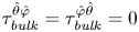 $\tau ^{{\hat {\theta }}{\hat {\varphi }}}_{\mathit {bulk}} = \tau ^{{\hat {\varphi }}{\hat {\theta }}}_{\mathit {bulk}} = 0$. The divergence of
 $\tau ^{{\hat {\imath }}{\hat {\jmath }}}$ is then
 \begin{equation}
\left.\begin{array}{c} \nabla_{\hat{j}} \tau^{{\hat{\theta}}{\hat{\jmath}}} = \dfrac{\partial_\theta\{\eta (1 + a\cos\theta)^3 \partial_\theta[u^{\hat{\theta}}/(1 + a\cos\theta)]\}} {r^2(1 + a \cos\theta)^2}\\
\quad + \dfrac{1}{r^2} \dfrac{\partial}{\partial \theta} \dfrac{\eta_v \partial_\theta [u^{\hat{\theta}}(1 + a \cos\theta)]} {1 + a \cos\theta},\\
\nabla_{\hat{j}} \tau^{{\hat{\varphi}}{\hat{\jmath}}} = \dfrac{\partial_\theta\{\eta (1 + a\cos\theta)^3 \partial_\theta[u^{\hat{\varphi}}/(1 + a\cos\theta)]\}} {r^2(1 + a \cos\theta)^2}. \end{array}\right\} \end{equation}
For the non-dissipative contributions to the pressure tensor, the divergence  $\nabla _{\hat {\jmath }} \boldsymbol{\mathsf{P}}^{{\hat {\imath }}{\hat {\jmath }}}_{\kappa }$ of the term involving surface tension can be evaluated using
 \begin{equation} \nabla_{\hat{\jmath}} \boldsymbol{\mathsf{P}}^{{\hat{\imath}}{\hat{\jmath}}}_{\kappa} = -\phi \kappa \nabla^{{\hat{\imath}}} {\rm \Delta} \phi. \end{equation}
Thus, the  ${\hat {\varphi }}$ component of the Cauchy equation reads as
 \begin{equation} \rho \left\{\frac{\partial u^{\hat{\varphi}}}{\partial t} + u^{\hat{\theta}} \frac{\partial_\theta[u^{\hat{\varphi}}(1 + a \cos\theta)]}{r(1 + a\cos\theta)} \right\} = \frac{\partial_\theta\{\eta (1 + a\cos\theta)^3 \partial_\theta[u^{\hat{\varphi}}/(1 + a\cos\theta)]\}} {r^2(1 + a \cos\theta)^2}, \end{equation}
while the  ${\hat {\theta }}$ component can be written as
 \begin{align} &\rho\left[\frac{\partial u^{\hat{\theta}}}{\partial t} + \frac{u^{\hat{\theta}}}{r} \frac{\partial u^{\hat{\theta}}}{\partial \theta} + \frac{(u^{\hat{\varphi}})^2 \sin\theta}{R(1 + a \cos\theta)}\right] + \frac{1}{r} \frac{\partial P_{b}}{\partial \theta} = \frac{\phi \kappa}{r^3} \frac{\partial}{\partial \theta} \left\{\frac{\partial_\theta[(1 + a \cos\theta)\partial_\theta \phi]} {1 + a \cos\theta}\right\} \nonumber\\ &\quad + \frac{\partial_\theta\{\eta (1 + a\cos\theta)^3 \partial_\theta[u^{\hat{\theta}}/(1 + a\cos\theta)]\}} {r^2(1 + a \cos\theta)^2} + \frac{1}{r^2} \frac{\partial}{\partial \theta}\left\{ \eta_v \frac{\partial_\theta [u^{\hat{\theta}}(1 + a \cos\theta)]} {1 + a \cos\theta}\right\}. \end{align}
To derive the energy equation (2.1c), the following contraction is useful:
 \begin{align} \tau^{{\hat{\imath}}{\hat{\jmath}}} \nabla_{\hat{\imath}} u_{\hat{\jmath}} &= \frac{1}{2 \eta} \tau_{\mathit{dyn}}^{{\hat{\imath}}{\hat{\jmath}}} \tau^\textrm{dyn}_{{\hat{\imath}}{\hat{\jmath}}} + \frac{1}{2\eta_v} \tau_{\mathit{bulk}}^{{\hat{\imath}}{\hat{\jmath}}} \tau^\textrm{bulk}_{{\hat{\imath}}{\hat{\jmath}}} \nonumber\\ &= \frac{1}{\eta} \left[(\tau^{{\hat{\theta}}{\hat{\theta}}}_{\mathit{dyn}})^2 + (\tau_{\mathit{dyn}}^{{\hat{\varphi}}{\hat{\theta}}})^2\right] + \frac{1}{\eta_v} (\tau_{\mathit{bulk}}^{{\hat{\theta}}{\hat{\theta}}})^2, \end{align}
where the properties 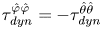 $\tau _{\mathit {dyn}}^{{\hat {\varphi }}{\hat {\varphi }}} = -\tau _{\mathit {dyn}}^{{\hat {\theta }}{\hat {\theta }}}$ and
 $\tau ^{{\hat {\theta }}{\hat {\theta }}}_{\mathit {bulk}} = \tau ^{{\hat {\varphi }}{\hat {\varphi }}}_{\mathit {bulk}}$ have been used. Thus, the energy equation can be written as
 \begin{align} &\rho \left(\frac{\partial e}{\partial t} + \frac{u^{\hat{\theta}}}{r} \frac{\partial e}{\partial \theta}\right) + \frac{P_{b}\partial_\theta[u^{\hat{\theta}}(1 + a \cos\theta)]} {r(1 + a \cos\theta)} \nonumber\\ &\quad = \frac{1}{r^2} \frac{\partial_\theta[(1 + a \cos\theta) k \partial_\theta T]} {1 + a\cos\theta} + \frac{1}{\eta} \left[(\tau^{{\hat{\theta}}{\hat{\theta}}}_{\mathit{dyn}})^2 + (\tau_{\mathit{dyn}}^{{\hat{\varphi}}{\hat{\theta}}})^2\right] + \frac{1}{\eta_v} (\tau_{\mathit{bulk}}^{{\hat{\theta}}{\hat{\theta}}})^2. \end{align}
Finally, on the torus, the Cahn–Hilliard equation, (2.12), reduces to
 \begin{equation} \frac{\partial \phi}{\partial t} + \frac{\partial_\theta[\phi u^{\hat{\theta}}(1 + a \cos\theta)]} {r(1 + a \cos\theta)} = \frac{M}{r^2} \frac{\partial_\theta[(1 + a\cos\theta)\partial_\theta \mu]} {1 + a \cos\theta}, \end{equation}
where the chemical potential is computed using
 \begin{equation} \mu = -A \phi(1- \phi^2) - \frac{\kappa}{r^2} \frac{\partial_\theta[(1 + a\cos\theta)\partial_\theta \phi]} {1 + a \cos\theta}.\end{equation}
3. Sound speed for perfect fluids
The first problem we study in this work is sound wave propagation for perfect fluids on the torus geometry. In fluids, sound waves provide the basic mechanism of information propagation. Many interesting phenomena involving the properties of sound wave propagation form the object of focus in acoustics. In addition, due to their fundamental importance, sound wave propagation should be considered as a first benchmark for any hydrodynamics solver. For perfect fluids, we neglect dissipative effects, such that the dynamic viscosity  $\eta$ and the heat conductivity
 $k$ can be taken to be zero. For simplicity, we will also set the surface tension parameter
 $\kappa$ and the mobility
 $M$ in the Cahn–Hilliard equation to zero.
Focussing on sound wave propagation along the poloidal ( $\theta$) direction of the torus, we will show that the sound waves exhibit a discrete spectrum of harmonics. The eigenfrequencies corresponding to these harmonics can be related to those of the standard Fourier harmonics for periodic domains, but, surprisingly, the eigenfrequencies corresponding to odd and even modes have different values, unlike for a planar geometry (Rieutord Reference Rieutord2015; Busuioc et al. Reference Busuioc, Ambruş, Biciuşcă and Sofonea2020). The eigenfunctions describing the spatial dependence also generalise from the usual harmonic sine and cosine basis to more complex odd and even functions. We determine the eigenfunctions using a perturbative approach, starting with the harmonic functions at zeroth order.
This section is structured as follows. The general solution for the propagation of longitudinal waves is presented in § 3.1. Then, two benchmark problems are proposed in §§ 3.2 and 3.3.
3.1. General solution
Let us consider small perturbations around a stationary, background state at density  $\rho _0$, internal energy
 $e_0$ and order parameter
 $\phi _0$, having bulk pressure
 $P_0 \equiv P_{b}(\rho _0, e_0, \phi _0)$
 \begin{equation} \rho = \rho_0(1 + \delta \rho), \quad e = e_0(1 + \delta e), \quad P_{b} = P_0(1 + \delta P), \quad \phi = \phi_0 + \delta \phi. \end{equation}
The perturbations in the pressure  $\delta P$ can be expressed as
 \begin{equation} \delta P = \frac{\rho_0 P_{\rho,0}}{P_0} \delta \rho + \frac{e_0 P_{e,0}}{P_0} \delta e + \frac{P_{\phi,0}}{P_0} \delta \phi, \end{equation}
where for brevity the following notation is introduced:
 \begin{equation} P_\rho = \frac{\partial P_{b}}{\partial \rho}, \quad P_e = \frac{\partial P_{b}}{\partial e}, \quad P_\phi = \frac{\partial P_{b}}{\partial \phi}. \end{equation}
The subscripts  $0$ in (3.2) indicate that the derivatives of the pressure are computed for the background state.
Assuming that the velocity components  $u^{\hat {\theta }}$ and
 $u^{\hat {\varphi }}$ are small, and neglecting all second-order terms of the perturbations introduced, the continuity (2.36), Cauchy (2.41) energy (2.43) and Cahn–Hilliard (2.44) equations reduce to
 \begin{equation} \left.\begin{array}{c@{}} \dfrac{\partial \delta \rho}{\partial t} + \dfrac{\partial_\theta {\mathcal{U}}}{r(1 + a \cos\theta)} = 0, \\ \dfrac{\partial {\mathcal{U}}}{\partial t} + \dfrac{P_0(1 + a \cos\theta)}{\rho_0 r} \dfrac{\partial \delta P}{\partial \theta} = 0, \\ \dfrac{\partial \delta \phi}{\partial t} + \dfrac{\phi_0 \partial_\theta \mathcal{U}}{r(1+ a \cos\theta)} = 0, \end{array}\right\} \end{equation}
while  $\partial _t u^{\hat {\varphi }} = 0$. Note that, in the above, we introduced the following notation:
 \begin{equation} {\mathcal{U}} = u^{\hat{\theta}} (1 + a \cos\theta). \end{equation}
Taking the time derivative of the second relation in (3.4) and replacing  $\delta P$ with (3.2) gives
 \begin{equation} \frac{\partial^2 {\mathcal{U}}}{\partial t^2} - \frac{c_{s,0}^2}{r^2} (1 + a \cos\theta) \frac{\partial}{\partial \theta} \left(\frac{1}{1 + a \cos\theta}\frac{\partial {\mathcal{U}}}{\partial \theta}\right) = 0. \end{equation}
Equation (3.6) represents the generalisation of the sound wave equation for axisymmetric flows on the torus geometry. We can recognise  $c_{s,0}$ as the sound speed corresponding to the background fluid parameters. In general,
 $c_s^2$ can be computed using
 \begin{equation} c_s^2 = P_\rho + \frac{P_{b}}{\rho^2} P_e + \frac{\phi}{\rho} P_\phi. \end{equation}
For the ideal gas,  $P_{b} = \rho k_B T / m$ and
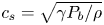 $c_s = \sqrt {\gamma P_{b} / \rho }$, where
 $\gamma = 1 + k_B / m c_v$ is the adiabatic index (e.g.
 $\gamma = 2$ for a monoatomic ideal gas with
 $2$ translational degrees of freedom). The isothermal regime can be recovered by setting
 $c_v \rightarrow \infty$ and
 $\gamma \rightarrow 1$. For the isothermal ideal fluid, we recover
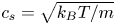 $c_s = \sqrt {k_B T / m}$.
Equation (3.6) can be solved using the method of separation of variables with the following ansatz:
 \begin{equation} {\mathcal{U}}(t, \theta) \rightarrow {\mathcal{U}}_n(t, \theta) = U_n(t) \Psi_n(\theta). \end{equation}
The index  $n$ reflects the fact that there are more than one possible solutions, corresponding to a discrete set of eigenvalues
 $\lambda _n$. The temporal function corresponds to simple harmonic oscillations of the form
 \begin{equation} \ddot{U}_n = - \lambda_n^2 \frac{c_{s,0}^2}{r^2} U_n. \end{equation}
The angular functions satisfy the differential equation
 \begin{equation} (1 + a \cos\theta) \frac{\textrm{d}}{\textrm{d}\theta}\left( \frac{1}{1 + a \cos\theta} \frac{\textrm{d}\Psi_n}{\textrm{d}\theta}\right) + \lambda_n^2 \Psi_n = 0.\end{equation}
The functions  $\Psi _n$ are twice differentiable periodic solutions with a discrete set of eigenvalues
 $\lambda _n$. Equation (3.10) has even and odd solutions, which we denote by
 $f_n(\theta )$ and
 $g_n(\theta )$. It can be shown that these functions are orthogonal with respect to the inner product, which is defined below for two functions
 $\psi (\theta )$ and
 $\chi (\theta )$
 \begin{equation} \langle \psi, \chi \rangle = \int_{0}^{2{\rm \pi}} \frac{\textrm{d}\theta}{2{\rm \pi}} \frac{\psi(\theta) \chi(\theta)}{1 + a \cos\theta}. \end{equation}
We seek solutions of unit norm, such that
 \begin{equation} \langle f_n, f_{n'}\rangle = \delta_{n,n'}, \quad \langle g_n, g_{n'} \rangle = \delta_{n,n'}, \quad \langle f_n, g_{n'}\rangle = 0. \end{equation}
The zeroth mode solution, corresponding to  $n = 0$ and
 $\lambda _0 = 0$, is straightforward to identify. The solution is a constant. Exploiting the condition of unit norm, we can use the following integral
 \begin{equation} \frac{1}{2{\rm \pi}} \int_{0}^{2{\rm \pi}} \frac{\textrm{d}\theta}{1 + a \cos\theta} = \frac{1}{\sqrt{1 - a^2}} \end{equation}
to obtain that
 \begin{equation} f_0(\theta) = (1 - a^2)^{1/4}. \end{equation}
There is no antisymmetric solution corresponding to  $n = 0$ and
 $\lambda _0 = 0$.
We will now discuss the subsequent values of  $\lambda _{c;n}$ and
 $\lambda _{s;n}$, the eigenvalues of the even (
 $\, f_n$) and odd (
 $g_n$) solutions. More specifically, the pairs
 $(\, f_n, \lambda _{c;n})$ and
 $(g_n, \lambda _{s;n})$ satisfy (3.10):
 \begin{equation} \left.\begin{array}{c@{}} \displaystyle (1 + a \cos\theta) \dfrac{\textrm{d}}{\textrm{d}\theta}\left( \dfrac{1}{1 + a \cos\theta} \dfrac{\textrm{d}f_n}{\textrm{d}\theta}\right) + \lambda_{c;n}^2 \, f_n = 0,\quad f_n(\theta) = f_n(2{\rm \pi} - \theta), \\[12pt] \displaystyle (1 + a \cos\theta) \dfrac{\textrm{d}}{\textrm{d}\theta}\left( \dfrac{1}{1 + a \cos\theta} \dfrac{\textrm{d}g_n}{\textrm{d}\theta}\right) + \lambda_{s;n}^2 g_n = 0,\quad g_n(\theta) = -g_n(2{\rm \pi} - \theta). \end{array}\right\} \end{equation}
We index the solutions incrementally such that  $f_{n+1}$ has an eigenvalue
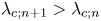 $\lambda _{c;n+1} > \lambda _{c;n}$, and similarly for the odd solutions.
Equation (3.10) can be solved analytically in the limit case  $a = 0$ (corresponding to an infinitely wide torus,
 $R \rightarrow \infty$). In this case, when
 $n > 0$, (3.10) yields the usual (normalised) harmonic basis encountered on a system with periodic coordinate
 $\theta$
 \begin{equation} f_n = \sqrt{2}\cos n\theta, \quad g_n = \sqrt{2}\sin n\theta. \end{equation}
Here,  $\lambda _{c;n} = \lambda _{s;n} = n$. For
 $n = 0$, (3.14) reduces to
 $f_0(\theta ) = 1$.
Another limit where the analytical solution is available is when  $a = 1$. In this case, the eigenfrequency spectrum is derived in SM:3.13 and SM:3.17 and is reproduced below, for convenience
 \begin{equation}\lambda_{c;n}^2 = n^2 - \frac{1}{4},\quad \lambda_{s;n}^2 = n(n+1). \end{equation}
The derivation and explicit form of the eigenfunctions for  $a=1$ are given in § SM:3.2.1 of the supplementary material.
For intermediate values of  $a$ (i.e. for
 $0 < a < 1$) and
 $\lambda _n^2 > 0$, there is no known analytic solution of (3.10). However, given that
 $a < 1$, it is reasonable to seek for the solutions in a perturbative manner. Starting from the
 $a = 0$ solution in (3.16), for a given value of
 $n$, we expect that the perturbation procedure will bring in harmonics corresponding to
 $n \pm 1$,
 $n \pm 2$, and so forth. The eigenvalues
 $\lambda _{c;n}$ and
 $\lambda _{s;n}$ travel along a continuous path from
 $\lambda _{c;n} = n$ to
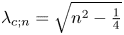 $\lambda _{c;n} = \sqrt {n^2 - \frac {1}{4}}$, and from
 $\lambda _{s;n} = n$ to
 $\lambda _{s;n} = \sqrt {n(n+1)}$, respectively, as
 $a$ goes from
 $0$ to
 $1$. The perturbative procedure is discussed in appendix B and the results for
 $1 \le n \le 4$ are given up to
 $O(a^9)$ in SM:3.3 of the supplementary material.
In general, the eigenvalues  $\lambda _{c;n}$ and
 $\lambda _{s;n}$ for the even and odd modes of the same order
 $n$ are not equal. As discussed in appendix B, the difference between
 $\lambda _{c;n}$ and
 $\lambda _{s;n}$ appears via terms of order
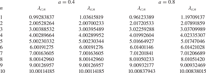
 $O(a^{2n})$. Table 1 shows the values of
 $\lambda _{c;n}$ and
 $\lambda _{s;n}$ obtained using high precision numerical integration for the cases
 $a = 0.4$ and
 $a = 0.8$. It can be seen that the difference between
 $\lambda _{c;n}$ and
 $\lambda _{s;n}$ decreases as
 $n$ is increased and
 $a$ is kept fixed, or as
 $n$ is kept fixed and
 $a$ is decreased. This is in contrast to the flat geometry, where the eigenvalues for the even and odd modes of the same order
 $n$ are always identical.


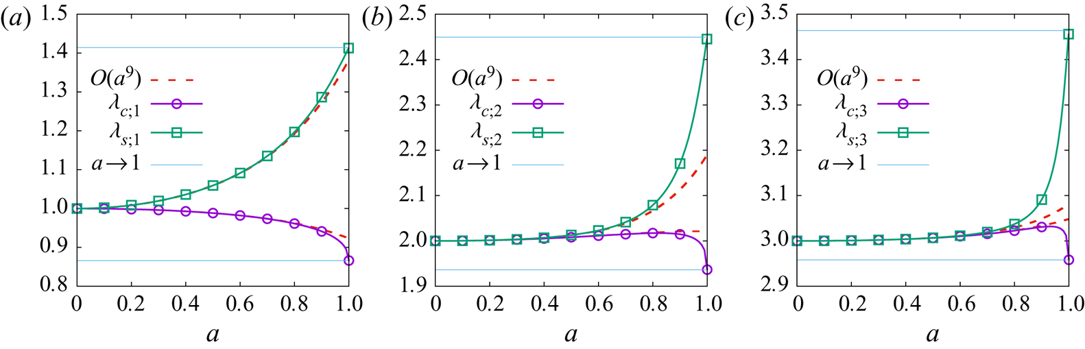
The dependence of  $\lambda _{c;n}$ and
 $\lambda _{s;n}$ on
 $a$ is revealed in figures 2(a)–2(c) for
 $n = 1$,
 $2$ and
 $3$. It can be seen that, as
 $a \rightarrow 1$,
 $\lambda _{c;n}$ also has a strong variation with
 $a$. However, overall the variation of
 $\lambda _{c;n}$ with
 $a$ is significantly milder than that of
 $\lambda _{s;n}$. For comparison, the dotted lines corresponding to the perturbative approximations up to
 $O(a^9)$, and the limits
 $\lim _{a\rightarrow 1} \lambda _{c;n} = \sqrt {n^2 - \frac {1}{4}}$ and
 $\lim _{a\rightarrow 1} \lambda _{s;n} = \sqrt {n(n+1)}$ are also shown.
The dependence of  $\lambda _{c;n}$ and
 $\lambda _{s;n}$ on
 $a$ for
 $n = 1$ (a),
 $2$ (b) and
 $3$ (c), respectively. The solid lines with symbols represent the numerically evaluated values of the eigenfrequencies, while the dotted lines show the perturbative approximations with terms up to
 $O(a^9)$. The horizontal lines show the
 $a = 1$ limits given in (3.17).

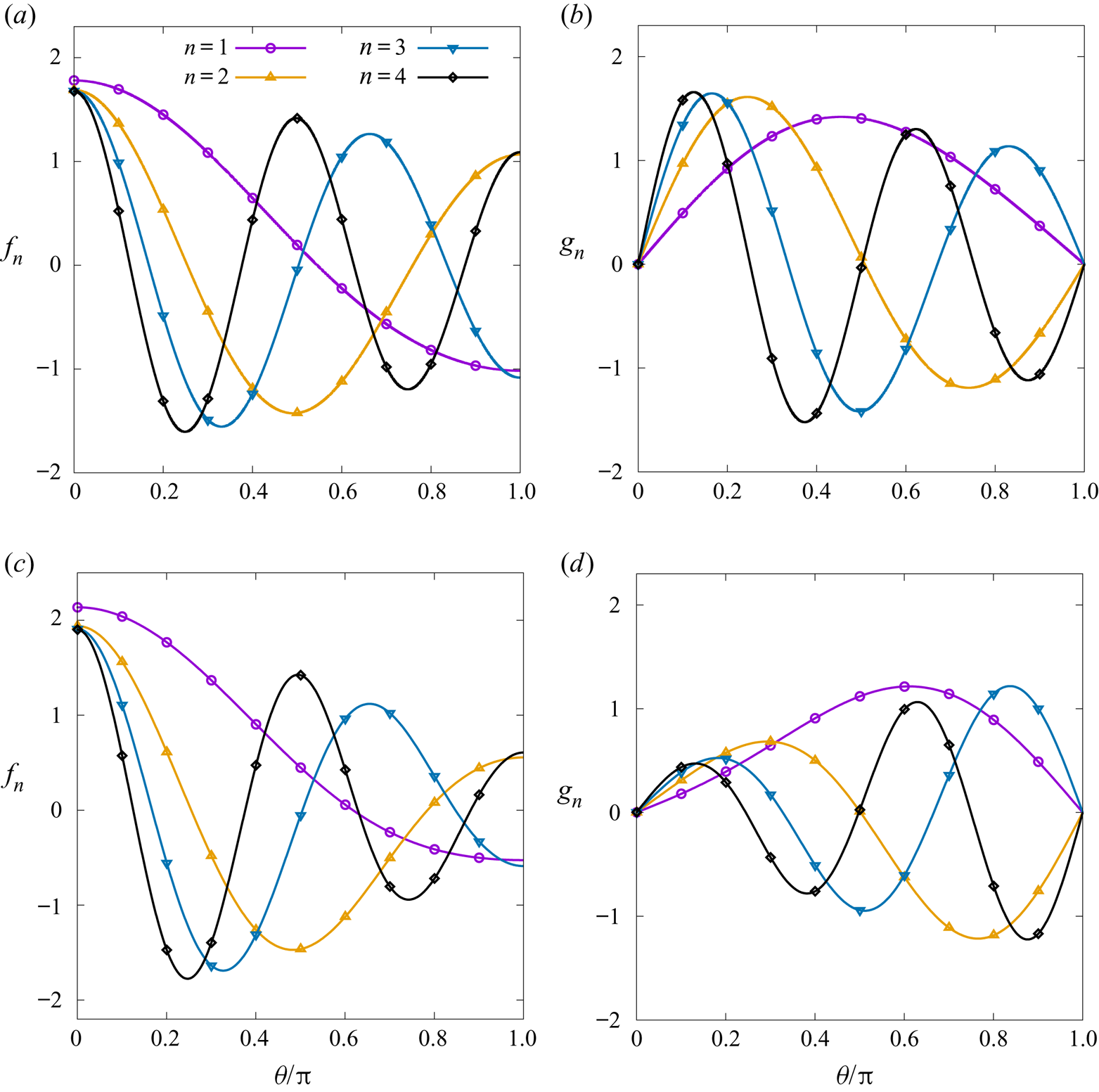
Figures 3(a) and 3(b) show the even and odd eigenfunctions  $f_n$ and
 $g_n$ corresponding to
 $1 \le n \le 4$ over the half-domain
 $0 \le \theta \le {\rm \pi}$ with
 $a = 0.4$. Similarly, figures 3(c) and 3(d) show
 $f_n$ and
 $g_n$ when
 $a = 0.8$. It can be seen that the amplitudes for the even harmonics
 $f_n$ become weaker towards
 $\theta = {\rm \pi}$ as
 $a$ is increased, while the amplitudes of the odd harmonics
 $g_n$ become weaker towards
 $\theta =0$.


Assuming that the functions  $\{\, f_n, g_n\}$ form a complete set, the fluid velocity can in general be written as
 \begin{equation} u^{\hat{\theta}}(t,\theta) = \frac{1}{1 + a \cos\theta} \sum_{n = 0}^\infty \left[U_{c;n}(t) f_n(\theta) + U_{s;n}(t) g_n(\theta)\right]. \end{equation}
Such an expansion is consistent when the inner product, (3.11), is dual to the following completeness relation:
 \begin{equation} \sum_{n = 0}^\infty [\, f_n(\theta) f_n(\theta') + g_n(\theta) g_n(\theta')] = 2{\rm \pi} (1 + a \cos\theta) \delta(\theta - \theta'). \end{equation}
Solving (3.9), it can be seen that the even and odd solutions for the temporal function (for  $n > 0$) correspond to simple harmonic oscillations
 \begin{equation} U_{c;n}(t) = U_{c;n;0} \cos\left( \omega_{c;n} t + \vartheta_{c;n}\right), \quad U_{s;n}(t) = U_{s;n;0} \sin\left( \omega_{s;n} t + \vartheta_{s;n}\right), \end{equation}
where  $\omega _{c;n} = \lambda _{c;n} c_s / r$ and
 $\omega _{s;n} = \lambda _{s;n} c_s / r$. The coefficients
 $U_{c;n;0}$ and
 $U_{s;n;0}$ and the phases
 $\vartheta _{c;n}$ and
 $\vartheta _{s;n}$ can be determined from the initial conditions
 \begin{equation} u^{\hat{\theta}}(0,\theta) = u^{\hat{\theta}}_0(\theta), \quad \dot{u}^{\hat{\theta}}(0, \theta) = -\frac{P_0}{\rho_0 r} \partial_\theta \delta P_0(\theta), \end{equation}
where  $u^{\hat {\theta }}_0(\theta )$ represents the initial velocity profile, while
 $\delta P_0(\theta ) = \delta P(0,\theta ) = (P_{\mathrm {b}}(0,\theta ) - P_0)/P_0$ represents the initial pressure fluctuations. Projecting the above equations onto
 $f_n$ and
 $g_n$ yields
 \begin{equation} \left.\begin{array}{c@{}}
\displaystyle\begin{pmatrix} U_{c;n;0} \cos \vartheta_{c;n} \\
U_{s;n;0} \sin \vartheta_{s;n} \end{pmatrix} =
\int_{0}^{2{\rm \pi}} \dfrac{\textrm{d}\theta}{2{\rm \pi}}
\begin{pmatrix} f_n \\ g_n \end{pmatrix}
u^{\hat{\theta}}_0(\theta), \\[12pt] \displaystyle
\begin{pmatrix} U_{c;n;0} \sin \vartheta_{c;n} \\
-U_{s;n;0} \cos \vartheta_{s;n} \end{pmatrix} =
\dfrac{P_0}{\rho_0 c_s} \int_{0}^{2{\rm \pi}}
\dfrac{\textrm{d}\theta}{2{\rm \pi}} \begin{pmatrix} f_n /
\lambda_{c;n} \\ g_n / \lambda_{s;n} \end{pmatrix}
\dfrac{\partial \delta P_0}{\partial \theta},
\end{array}\right\} \end{equation}
where the last equation applies only for  $n > 0$. It is worth noting that the
 $n = 0$ term, corresponding to the incompressible flow profile
 \begin{equation} \frac{U_{c;0} \, f_0(\theta)}{1 + a \cos\theta},\end{equation}
is time-independent and its amplitude,  $U_{c;0}$, is preserved at all times. Thus, numerical methods developed for hydrodynamics on curved surfaces should ensure the preservation of the above profile. In the Cartesian geometry, the incompressible flow profile along a single axis is a constant background velocity, which should be preserved due to the Galilean invariance of the theory.
For the rest of this work, we employ expansions of up to  $a^9$ of the eigenfunctions, eigenvalues and all related quantities. These expansions are given in SM:3.3 of the supplementary material. Although some expansions converge faster than the others, for consistency reasons, we choose to employ the same order of expansion for all quantities involved.
3.2. First benchmark: constant initial flow
We now formulate a simple numerical experiment that can be used to benchmark the capabilities of numerical methods to capture sound wave propagation on curved geometries. The simplest configuration giving rise to sound wave propagation corresponds to
 \begin{equation} u^{\hat{\theta}}_0(\theta) = U_0, \quad \delta P_0(\theta) = 0, \end{equation}
with  $U_0$ a constant. Since the initial velocity profile is symmetric and the initial pressure is constant,
 $\vartheta _{c;n} = 0$ and
 $U_{s;n;0} = 0$. To calculate the coefficients of the even modes, we take advantage of the projections introduced in (3.22). The fluid velocity can then be written as
 \begin{equation} \left.\begin{array}{c@{}}
\displaystyle u^{{\hat{\theta}}}(t, \theta) = \dfrac{1}{1 +
a \cos\theta} \left[U_0 \sqrt{1 - a^2} + \sum_{n =
1}^\infty U_{c;n}(t) f_n(\theta) \right],\\
\displaystyle U_{c;n}(t) = U_0 I_{c;0;n}
\cos\left(\dfrac{c_{s,0} \lambda_{c;n}}{r}t\right),
\end{array}\right\}
\end{equation}
where the eigenvalues  $\lambda _{c;n}$ are given up to ninth order with respect to
 $a$ in SM:3.3, and the integrals
 $I_{*;m; n}$ are defined as
 \begin{equation} I_{c; m; n} = \int_0^{2{\rm \pi}} \frac{\textrm{d}\theta}{2{\rm \pi}} \frac{f_n(\theta)}{(1 + a \cos\theta)^m}, \quad I_{s; m; n} = \int_0^{2{\rm \pi}} \frac{\textrm{d}\theta}{2{\rm \pi}} \frac{g_n(\theta) \sin\theta}{(1 + a \cos\theta)^m}. \end{equation}
In this section, we only need the case with  $m = 0$, for which
 $I_{c;0;0} = (1-a^2)^{1/4}$, while the first integrals (
 $1\leq n\leq 4$) are given up to ninth order with respect to
 $a$ in SM:3.3 of the supplementary material. The integrals
 $I_{s;0;n}$ of the odd functions will be employed later, in § 3.3.
In order to perform numerical simulations, we consider a non-dimensionalisation of physical quantities with respect to the background fluid parameters, such that  $\rho _0 = T_0 = P_0 = 1$. Focussing on the torus with
 $a = r/ R = 0.4$, we take the reference length scale such that
 $R = 2$. Setting the reference velocity naturally to
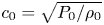 $c_0 = \sqrt {P_0 / \rho _0}$, we initialise the velocity by setting
 $u^{\hat {\theta }}_0(\theta ) = U_0 = 10^{-5}$ in (3.24). Using the aforementioned reference velocity, the non-dimensional sound speed is
 $c_{s,0} = 1$ for the isothermal case and
 $c_{s,0} = \sqrt {2}$ for the thermal case when the adiabatic index is
 $\gamma = 2$. In addition, we also consider an isothermal multicomponent fluid for which the sound speed is given by
 \begin{equation} c_{s,0}^2 = \frac{k_B T_0}{m} - \frac{A \phi_0^2}{\rho_0}(1 - 3 \phi_0^2). \end{equation}
We choose  $A = 1$; and consider values of
 $\phi _0 = 1$ and
 $\phi _0 = 0.8$, which are outside the spinodal region,
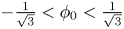 $-\frac {1}{\sqrt {3}} < \phi _0 < \frac {1}{\sqrt {3}}$. The resulting sound speeds are summarised in table 2.
Sound speed and angular frequencies  $\omega _n = c_{s,0} \lambda _{c;n} / r$ for the first three harmonics of the oscillatory motion on the torus with
 $a = 0.4$, considered in figure 4.

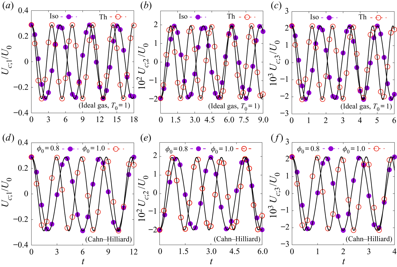
For the four cases above with differing sound speeds, the system is evolved between  $0 \le t \le 18$ on a grid with
 $N_\theta = 320$ equidistant nodes and a time step
 $\delta t = 5 \times 10^{-4}$. The velocity profile is projected onto the basis functions
 $f_1$,
 $f_2$ and
 $f_3$, as given in SM:3.3a, SM:3.3b and SM:3.3c of the supplementary material, respectively. The simulation results are shown using dashed lines and symbols in figure 4. For comparison, the corresponding analytical solutions in (3.25) are shown in solid lines in figure 4. The angular frequencies,
 $\omega _n = c_{s,0} \lambda _{c;n} / r$, for the first three harmonics are reported for convenience in table 2. The agreement between the analytical and numerical results is excellent. It is also worth noting that the angular frequencies on the torus differ from those for the flat geometry, and the deviations become more significant with increasing
 $a$.
Comparison between the numerical results (symbols) and analytical predictions (solid lines) for the evolution of  $U_{c;n}(t)/U_0$, as given in (3.25). The first row (a–c) is for isothermal (Iso) and thermal (Th) ideal fluids, while the second row (d–f) is for Cahn–Hilliard multicomponent fluid. The integrals
 $I_{c;0;n}$ given in SM:3.3 have the values of
 $I_{c;0;1} \simeq 0.288$ (a,d);
 $I_{c;0;2} \simeq -0.0195$ (b,e); and
 $I_{c;0;3} \simeq 0.00216$ (c, f).

3.3. Second benchmark test: even and odd initial conditions
The purpose of the second test is to highlight the difference in the period corresponding to the propagation of even and odd perturbations. As highlighted in figure 2, the difference in the frequencies for the even and odd modes increases as  $a$ is increased. For this reason, in this example we consider
 $a = 0.8$. According to table 1, the ratio
 $\lambda _{s;1} / \lambda _{c;1} \simeq 1.25$, therefore the
 $n = 1$ odd mode should exhibit
 $5$ periods for every
 $4$ periods of the
 $n = 1$ even mode.
We consider two initial conditions, corresponding to even and odd initial velocity profiles
 \begin{equation} u^{\hat{\theta}}_{0;\mathit{even}}(\theta) = U_0 \cos\theta, \quad u^{\hat{\theta}}_{0;\mathit{odd}}(\theta) = U_0 \sin\theta, \end{equation}
where  $U_0$ is the (constant) initial amplitude. As before, the initial pressure perturbation is assumed to vanish, i.e.
 $\delta P_{0;\mathit {even}}(\theta ) = \delta P_{0;\mathit {odd}}(\theta ) = 0$. According to (3.22), this implies that the offset angles can be taken as
 $\vartheta _{c;n} = 0$ and
 $\vartheta _{s;n} = {\rm \pi}/ 2$. Furthermore, since
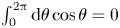 $\int _0^{2{\rm \pi} } \textrm {d}\theta \cos \theta = 0$, the coefficient
 $U_{c;n;0}^{\mathit {even}}$ of the zeroth mode (corresponding to
 $n = 0$) vanishes. This allows the velocity to be expanded in the two cases as follows:
 \begin{equation} \left.\begin{array}{c@{}} \displaystyle u^{\hat{\theta}}_{\mathit{even}}(t, \theta) = \sum_{n = 1}^\infty \dfrac{U_{c;n;0}^{\mathit{even}} \,f_n(\theta)}{1 + a \cos\theta} \cos(\omega_{c;n;0} t),\\[12pt] \displaystyle u^{\hat{\theta}}_{\mathit{odd}}(t, \theta) = \sum_{n = 1}^\infty \dfrac{U_{s;n;0}^{\mathit{odd}} g_n(\theta)}{1 + a \cos\theta} \cos(\omega_{s;n;0} t), \end{array}\right\} \end{equation}
where  $U_{s;n;0}^{\mathit {even}} = U_{c;n;0}^{\mathit {odd}} = 0$, while
 \begin{equation} \left.\begin{array}{c@{}} \displaystyle U^{\mathit{even}}_{c;n;0} = U_0 \int_0^{2{\rm \pi}} \dfrac{\textrm{d}\theta}{2{\rm \pi}} f_n(\theta) \cos\theta = U_0 \dfrac{\lambda_{c;n}^2}{a(2-\lambda_{c;n}^2)} I_{c;0,n},\\[12pt] \displaystyle U^{\mathit{odd}}_{s;n;0} = U_0 \int_0^{2{\rm \pi}} \dfrac{\textrm{d}\theta}{2{\rm \pi}} g_n(\theta) \sin\theta = U_0 I_{s;0;n}, \end{array}\right\} \end{equation}
where the first relation follows from noting that  $\cos \theta = a^{-1}(1 + a \cos \theta ) - a^{-1}$, while the integral
 $I_{c;-1;n}$ can be expressed in terms of
 $I_{c;0;n}$ by multiplying the first line of (3.15) with
 $(1 + a \cos \theta )/2{\rm \pi}$ and integrating with respect to
 $\theta$
 \begin{equation} I_{c;-1;n} = \int_0^{2{\rm \pi}} \frac{\textrm{d}\theta}{2{\rm \pi}} (1 + a \cos\theta) f_n(\theta) = \frac{2}{2-\lambda_{c;n}^2} I_{c;0;n}. \end{equation}
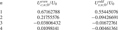
As can be seen from table 3, at  $a = 0.8$, the coefficient of the
 $n = 1$ mode is dominant. For the even initial conditions, the amplitude of the
 $n = 2$ mode is almost a third of the amplitude of the
 $n = 1$ mode, thus it can be expected that a modulation due to this mode will show up in the solution. This is less important for the odd initial conditions, since
 $U^{\mathit {odd}}_{s;2;0}$ is almost
 $6$ times smaller in magnitude than
 $U^{\mathit {odd}}_{s;1;0}$.
Values of the normalised amplitudes  $U^{\mathit {even}}_{c;n;0}/U_0$ and
 $U^{\mathit {odd}}_{s;n;0}/U_0$ defined in (3.30) for
 $a = 0.8$ and
 $1 \le n \le 4$.

We now consider an ideal perfect thermal fluid with  $\gamma = 2$ and employ the non-dimensionalisation according to which
 $\rho _0 = T_0 = P_0 = 1$,
 $R = 2$ (
 $r = 1.6$ such that
 $a = 0.8$), and
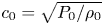 $c_0 = \sqrt {P_0 / \rho _0}$. The constant in (3.28) is set to
 $U_0 = 10^{-5}$. In this case, the angular frequency for the first even mode is
 $\omega _{c;1} = c_{s;0} \lambda _{c;1} / r \simeq 0.85$ and the time required for
 $4$ periods for this mode is
 $8{\rm \pi} / \omega _{c;1} \simeq 29.58$. The angular frequency for the first odd mode is
 $\omega _{s;1} = c_{s;0} \lambda _{s;1} / r \simeq 1.06$ and the time required for
 $5$ periods for this mode is
 $10{\rm \pi} / \omega _{s;1} \simeq 29.69$. We thus perform simulations covering the time domain
 $0 \le t \le 30$, using
 $N_{\theta } = 320$ nodes distributed equidistantly along the
 $\theta$ direction and a time step
 $\delta t = 10^{-3}$. The velocity configuration is saved every
 $100$ time steps, yielding a total of
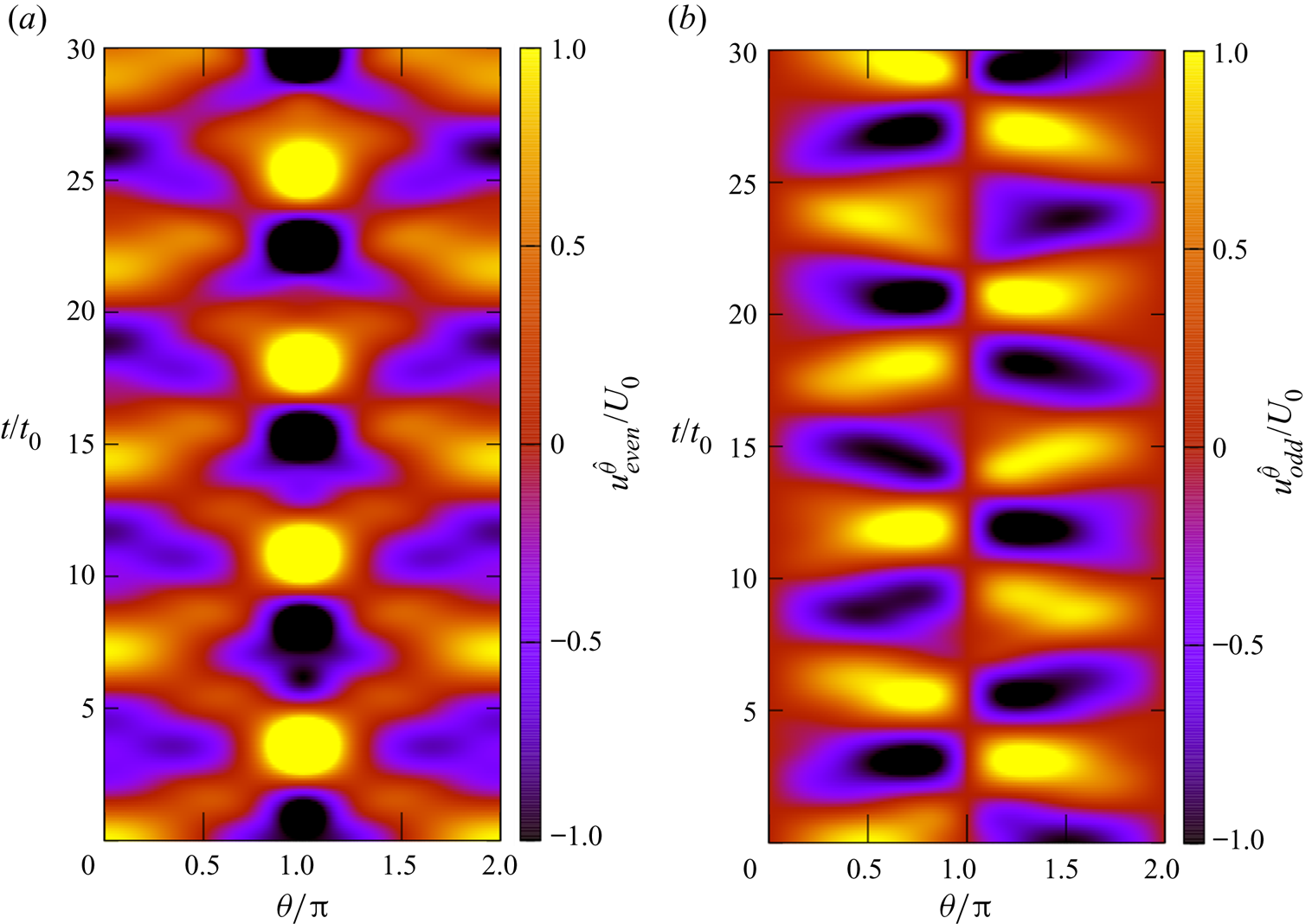
 $300$ snapshots, which are arranged in time lapses, as shown in figures 5(a) and 5(b). The ratio
 $u^{\hat {\theta }}/U_0$ is represented using a colour map, which is truncated to the values
 $[-1,1]$ for better visibility. It can be seen that the number of (quasi-)periods for the even and odd initial conditions are
 $4$ and
 $5$, as predicted based on the values of
 $\lambda _{c;1}$ and
 $\lambda _{s;1}$, respectively.
Time evolution of  $u^{\hat {\theta }}_{\mathit {even}} / U_0$ (a) and
 $u^{\hat {\theta }}_{\mathit {odd}} / U_0$ (b), defined in (3.29) on the torus with
 $a = 0.8$. The horizontal axis represents the angular coordinate along the poloidal direction, normalised with respect to
 ${\rm \pi}$. The vertical axis shows the time coordinate
 $t$, normalised with respect to
 $t_0 = R / 2 c_0$, where
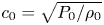 $c_0 = \sqrt {P_0 /\rho _0}$ is the reference speed. The colour map represents the value of
 $u^{\hat {\theta }}/U_0$ and is truncated to the interval
 $[-1,1]$.

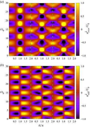
Finally, we discuss the emergence of the apparent periodicity breakdown observed in figures 5(a) and 5(b) for the even and odd initial conditions considered in this section. Figure 6 shows the analytic solutions for  $u^{\hat {\theta }}_{\mathit {even}}$ (a) and
 $u^{\hat {\theta }}_{\mathit {odd}}$ (b) derived in (3.29), truncated at
 $n = 1$ (left),
 $2$ (middle) and
 $3$ (right). We note that the amplitude of the zeroth-order harmonic vanishes when the initial state is prepared according to (3.28). The resulting configurations for different truncations are separated using dashed vertical green lines. It can be seen that the first-order harmonic exhibits the fundamental periodicity observed also in figure 5. Adding the second harmonic produces a visible disturbance since the amplitude ratios
 $U_{c;2;0} / U_{c;1;0} \simeq 0.324$ and
 $U_{s;2;0} / U_{s;1;0} \simeq -0.170$ are non-negligible. Because the ratios
 $\omega _{c;2} / \omega _{c;1} \simeq 2.099$ and
 $\omega _{s;2} / \omega _{s;1} \simeq 1.737$ are irrational numbers, the resulting configurations become pseudo-periodic. This is different from the flat geometry case where the ratios are integers, thereby conserving the periodicity of the solution. The addition of the third-order harmonic has a significantly milder effect, since the ratios
 $U_{c;3;0} / U_{c;1;0} \simeq -0.057$ and
 $U_{s;3;0} / U_{s;1;0} \simeq -0.030$ are small. Therefore, the middle configuration presented in figure 6 already provides a reasonable approximation of the configurations observed in figure 5.
Analytic solutions for 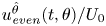 $u^{\hat {\theta }}_{\mathit {even}}(t,\theta ) / U_0$ (a) and
 $u^{\hat {\theta }}_{\mathit {odd}}(t,\theta ) / U_0$ (b), reconstituted via (3.29) using the harmonics up to
 $n = 1$ (left of each panel),
 $2$ (middle of each panel) and
 $3$ (right of each panel).

4. Viscous fluid: shear wave damping
In this section, we address the equivalent on the torus of a standard benchmark problem for viscous flow solvers. On the flat geometry, the shear wave set-up typically consists of a system which is homogeneous in two directions, say the  $y$ and
 $z$ axes. However, the fluid velocity in one of the directions, say the
 $y$ component, varies with respect to the
 $x$ axis. Due to this dependence, layers which are adjacent with respect to the
 $x$ direction travel at different velocities along the
 $y$ direction. Due to friction, the velocity difference between two such adjacent layers experiences a damping which is controlled by the kinematic viscosity of the fluid and is induced via the viscous part of the stress tensor. In the present case of the torus geometry, we consider that the poloidal component
 $u^{\hat {\theta }}$ of the fluid velocity vanishes, while its azimuthal component
 $u^{\hat {\varphi }}$ varies in magnitude as a function of the poloidal angle
 $\theta$.
This section is structured as follows. In § 4.1, the general solution for the shear wave damping problem on the torus is obtained. Sections 4.2 and 4.3 discuss two benchmark problems proposed in this context.
4.1. General solution
For the torus geometry, we consider the axisymmetric flow of an ideal, single-component fluid with vanishing poloidal velocity ( $u^{\hat {\theta }} = 0$). In this case, the linearised limit of the
 $\varphi$ component of the Cauchy equation (2.41a) reads
 \begin{equation} \partial_t u^{\hat{\varphi}} = \frac{\nu}{r^2(1 + a \cos\theta)^2} \frac{\partial}{\partial \theta} \left[ (1 + a \cos\theta)^3 \frac{\partial}{\partial \theta} \left( \frac{u^{\hat{\varphi}}}{1 + a\cos\theta}\right)\right], \end{equation}
with  $\rho \simeq \rho _0 = \textrm {const}$ and
 $P \simeq P_0 = \textrm {const}$. In the above,
 $\nu$ represents the kinematic viscosity, which we assume to be constant. The above equation can be solved using separation of variables by letting
 \begin{equation} u^{\hat{\varphi}}(t, \theta) \rightarrow u_n^{\hat{\varphi}}(t, \theta) = V_n(t) \Lambda_n(\theta) (1 + a \cos\theta). \end{equation}
Under this separation, the time-dependent amplitude satisfies the equation
 \begin{equation} \partial_t V_n(t) = -\frac{\nu \chi_n^2}{r^2} V_n(t) \Rightarrow V_n(t) = V_{n,0} \,\textrm{e}^{-\nu \chi_n^2 t / r^2}, \end{equation}
where  $\chi _n^2$ is a constant. The spatial component in (4.2),
 $\Lambda _n(\theta )$, satisfies
 \begin{equation} \frac{1}{(1 + a \cos\theta)^3} \frac{\partial}{\partial \theta} \left[ (1 + a \cos\theta)^3 \frac{\partial \Lambda_n}{\partial \theta} \right] + \chi_n^2 \Lambda_n = 0.\end{equation}
Similar to the problem discussed in the previous section, the above equation admits even and odd solutions, which we denote via  $F_n(\theta )$ and
 $G_n(\theta )$, respectively. The index
 $n$ labels the discrete eigenmodes of (4.4). We label the eigenvalues
 $\chi _{c;n}$ and
 $\chi _{s;n}$ for the even and odd modes, such that
 \begin{equation} \left.\begin{array}{c@{}}
\displaystyle \dfrac{1}{(1 + a \cos\theta)^3}
\dfrac{\partial}{\partial \theta} \left[ (1 + a
\cos\theta)^3 \dfrac{\partial F_n}{\partial \theta} \right]
+ \chi_{c;n}^2 F_n = 0,\\ \displaystyle \dfrac{1}{(1
+ a \cos\theta)^3} \dfrac{\partial}{\partial \theta} \left[
(1 + a \cos\theta)^3 \dfrac{\partial G_n}{\partial \theta}
\right] + \chi_{s;n}^2 G_n = 0.
\end{array}\right\} \end{equation}
It can be shown that the modes corresponding to different indices  $n$ and
 $n'$ are orthogonal. We choose the overall normalisation constants by imposing unit norm with respect to the inner product,
 $\langle F_n, F_{n'}\rangle = \langle G_n, G_{n'} \rangle = \delta _{n,n'}$. For two arbitrary functions
 $\Psi$ and
 $\Phi$, the inner product is defined as
 \begin{equation} \langle \Psi, \Phi \rangle = \frac{1}{2{\rm \pi}} \int_0^{2{\rm \pi}} \textrm{d}\theta (1 + a \cos\theta)^3 \Psi(\theta) \Phi(\theta).\end{equation}
The solution of (4.4) corresponding to  $n = 0$ and
 $\chi = 0$ is even, being given by
 \begin{equation} F_0 = \left[1 + \frac{3a^2}{2} \right]^{-1/2}. \end{equation}
When  $a = 0$, the eigenvalues are
 $\chi _{c;n}^2 = \chi _{s;n}^2 = n^2$, while the eigenmodes are given through
 \begin{equation} F_n(\theta) = \sqrt{2} \cos(n\theta), \quad G_n(\theta) = \sqrt{2} \sin(n\theta), \end{equation}
as was the case in § 3. When  $a = 1$, the eigenvalues are derived in SM:3.20 and are reproduced below, for convenience
 \begin{equation} \chi_{c;n} = \sqrt{n(n + 3)}, \quad \chi_{s;n} = \sqrt{(n + \tfrac{5}{2})(n - \tfrac{1}{2})}. \end{equation}
The eigenfunctions and the detailed procedure used to obtain them are given in § SM:3.2.2 of the supplementary material.
When  $0 < a < 1$, the eigenmodes can be obtained as power series with respect to
 $a$, as detailed in appendix B. The eigenfunctions
 $F_n$ and
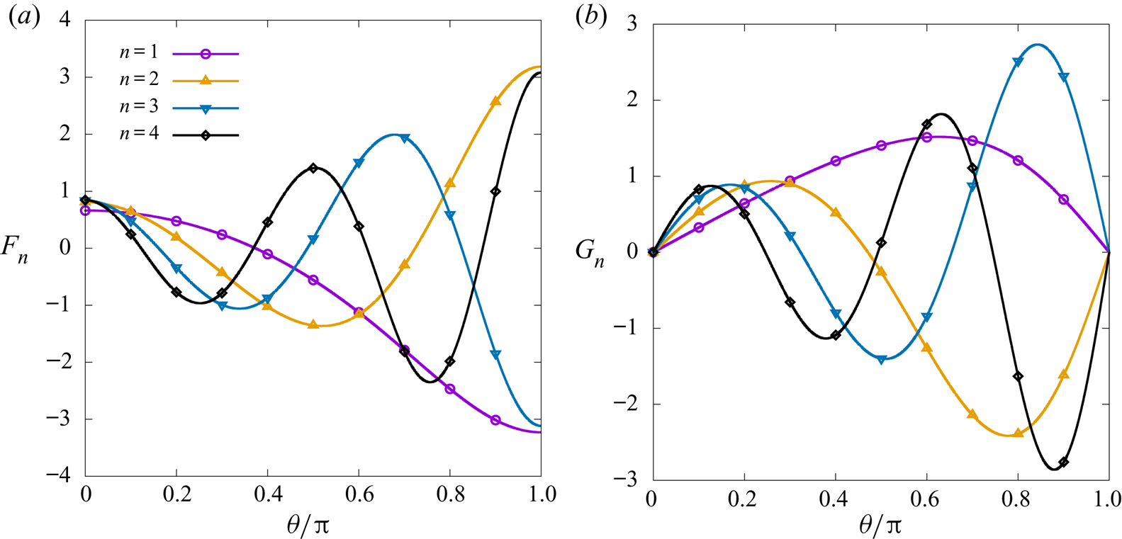
 $G_n$ are depicted graphically in figure 7 for
 $a = 0.4$ and
 $1 \le n \le 4$. The eigenvalues
 $\chi _n^2$ can be obtained following the same perturbative procedure as described in the previous section. As in the inviscid case, the difference between the eigenvalues corresponding to the
 $n$th odd and even modes appear at
 $O(a^{2n})$, as further discussed in appendix B. The dependence of
 $\chi _{*;n}$ (
 $* \in \{c,s\}$,
 $1 \le n \le 3$) on
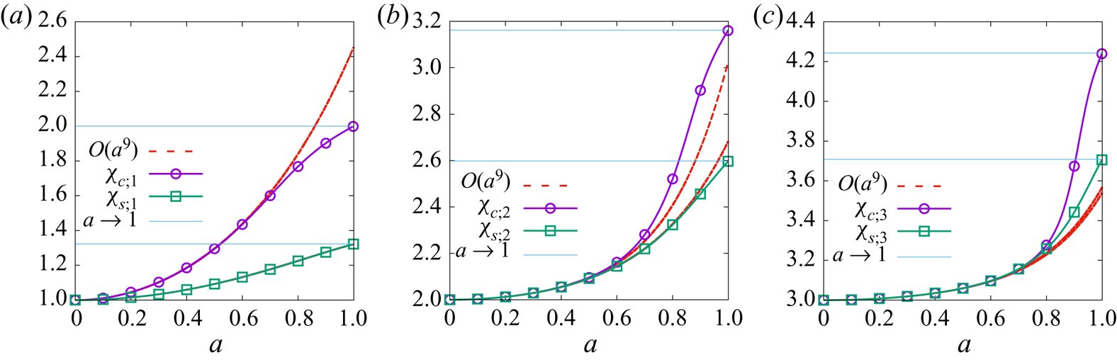
 $a$ is shown in figure 8, obtained using high precision numerical integration. It can be seen that all eigenvalues exhibit a monotonic increase with respect to
 $a$ and the eigenvalues
 $\chi _{c;n}$ corresponding to the even modes become significantly larger than those corresponding to the odd modes as
 $a \rightarrow 1$, as indicated in (4.9). The dotted lines correspond to the perturbative approximations up to
 $O(a^9)$. This behaviour is contrary to that of the eigenvalues seen in the inviscid case, shown in figure 2. In the inviscid case, the eigenvalues corresponding to the odd modes,
 $\lambda _{s;n}$, are generally larger than those corresponding to the even modes. Moreover,
 $\lambda _{c;n}$ has a non-monotonic behaviour, increasing with
 $a$ at small
 $a$ (for
 $n > 1$) and decreasing as
 $a \rightarrow 1$.
The even and odd eigenfunctions  $F_n$ (a) and
 $G_n$ (b) of (4.5), summarised in SM:3.4, with
 $a = 0.4$ for
 $n = 1$,
 $2$,
 $3$ and
 $4$. The eigenvalues corresponding to
 $n = 1$,
 $2$,
 $3$ and
 $4$ are
 $\chi _{c;n} \simeq 1.185$,
 $2.055$,
 $3.035$ and
 $4.026$ for the even modes, and
 $\chi _{s;n} \simeq 1.060$,
 $2.054$,
 $3.035$ and
 $4.026$ for the odd modes.

The dependence of  $\chi _{c;n}$ and
 $\chi _{s;n}$ on
 $a$ for (a)
 $n = 1$, (b)
 $n = 2$ and (c)
 $n = 3$. The dotted lines show the perturbative approximations in SM:3.4 with terms up to
 $O(a^9)$.

Combining the solutions for the time and angular dependences, the general solution can be written as
 \begin{equation} \left.\begin{array}{c@{}} \displaystyle u^{\hat{\varphi}}(t, \theta) = (1 + a \cos\theta) \sum_{n = 0}^\infty \left[ V_{c;n}(t) F_n(\theta) + V_{s;n}(t) G_n(\theta)\right], \\[12pt] \displaystyle V_{c;n}(t) = V_{c;n;0} \,\textrm{e}^{-\nu \chi_{c;n}^2 t/r^2}, \quad V_{s;n}(t) = V_{s;n;0}\,\textrm{e}^{-\nu \chi_{s;n}^2 t/r^2}. \end{array}\right\} \end{equation}
The amplitudes  $V_{c;n;0}$ and
 $V_{s;n;0}$ can be computed by integrating over the velocity profile at initial time,
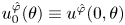 $u^{\hat {\varphi }}_0(\theta ) \equiv u^{\hat {\varphi }}(0, \theta )$
 \begin{equation} \begin{pmatrix} V_{c;n;0} \\ V_{s;n;0} \end{pmatrix} = \int_0^{2{\rm \pi}} \frac{\textrm{d}\theta}{2{\rm \pi}} (1 + a \cos\theta)^2 u^{\hat{\varphi}}_0(\theta) \begin{pmatrix} F_n(\theta) \\ G_n(\theta) \end{pmatrix}. \end{equation}
4.2. First benchmark: constant initial flow
To verify the analytical theory developed in this section and to allow comparisons against our numerical solutions, we consider a specific example where the fluid on the torus has an initially constant velocity profile
 \begin{equation} u^{{\hat{\varphi}}}_0(\theta) = V_0. \end{equation}
In this case, it can be seen that the odd coefficients  $V_{s;n;0}$ vanish, while the even coefficients can be computed as follows:
 \begin{align} V_{c;n;0} &= V_0 \int_0^{2{\rm \pi}} \frac{\textrm{d}\theta}{2{\rm \pi}} (1 + a \cos\theta)^2 F_n(\theta)\nonumber\\ &= V_0 \left[ \frac{6}{(2 + \chi_{c;n}^2)^2} - \frac{1 - a^2}{2 + \chi_{c;n}^2}\right] {\mathcal{I}}_{c;n}. \end{align}
The second line in (4.13) is obtained by multiplying the first line in (4.5) with  $(1 + a \cos \theta )^2/2{\rm \pi}$ and integrating with respect to
 $\theta$. For convenience, we also introduced
 \begin{equation} {\mathcal{I}}_{c;n} = \int_0^{2{\rm \pi}} \frac{\textrm{d}\theta}{2{\rm \pi}} F_n(\theta), \quad {\mathcal{I}}_{s;n} = \int_0^{2{\rm \pi}} \frac{\textrm{d}\theta}{2{\rm \pi}} \sin\theta G_n(\theta). \end{equation}
The result for  $n = 0$ is exact:
 ${\mathcal {I}}_{c;0} = (1 + 3a^2 / 2)^{-1/2}$ and
 $V_{c;0;0} = V_0 (1+a^2/2)/ \sqrt {1 + 3a^2/2}$. For
 $1\leq n \leq 4$, the power series approximations of the
 ${\mathcal {I}}_{c;n}$ integrals can be found in SM:3.4 of the supplementary material.
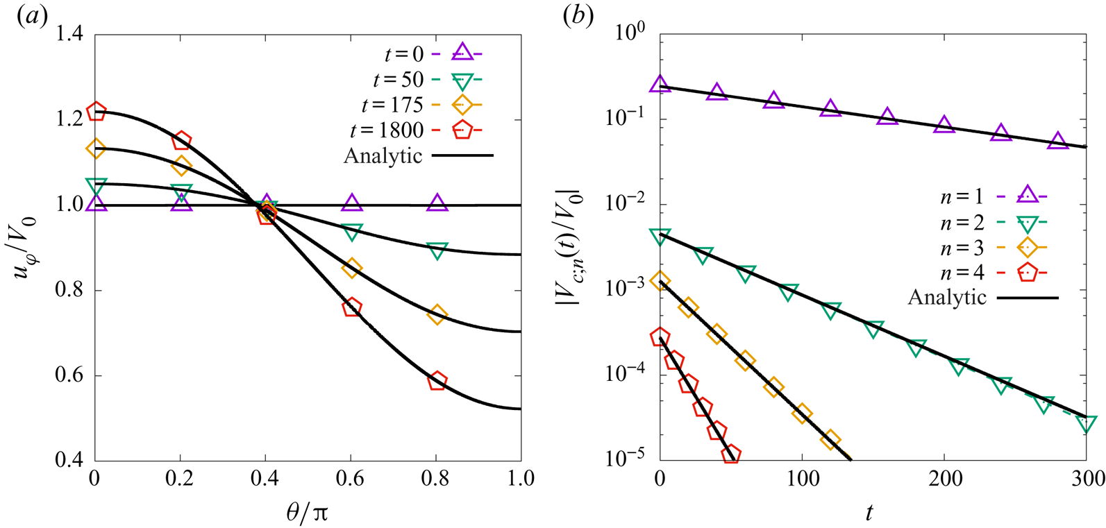
Figure 9(a) shows the numerical solution (dotted lines and points) and the analytic results obtained above (solid lines) for the fluid velocity in the azimuthal direction at four different values of the time coordinate. The agreement is excellent. We used an ideal, isothermal fluid with initial constant density  $\rho _0 = 1$ and constant temperature
 $T_0 = 1$, on a grid with
 $N_\theta = 320$ equidistant points and a time step of
 $\delta t = 5 \times 10^{-3}$. The reference speed is taken as
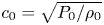 $c_0 = \sqrt {P_0 / \rho _0}$, where
 $P_0 = \rho _0 k_B T_0 / m$ is the reference pressure and
 $m$ is the particle mass. The kinematic viscosity is taken to be
 $\nu = 2.5 \times 10^{-3}$ with respect to the reference value
 $\nu _0 = c_0 L_0$, where
 $L_0 = R / 2$ is the reference length. With this convention, the non-dimensional torus parameters are
 $R = 2$ and
 $r = 0.8$, while the initial velocity amplitude in (4.12) is
 $V_0 = 10^{-5}$. Since the damping in (4.3) depends only on the fluid viscosity, the same results can be obtained when considering the thermal or the Cahn–Hilliard non-ideal fluids.
(a) Time evolution of the ratio  $u^{\hat {\varphi }}/V_0$ of the azimuthal velocity
 $u^{\hat {\varphi }}$ initialised according to (4.12), where
 $V_0$ is the initial amplitude. (b) Time evolution of the amplitudes
 $V_{c;n}(t)$ (
 $1 \le n \le 4$). The numerical results are shown with dotted lines and points, while the analytic prediction is summing only the terms with
 $0 \le n \le 4$ in (4.10). The torus radii ratio is
 $a = 0.4$.

The amplitudes of the harmonics are extracted from the numerical solution by means of the orthogonality relation, (4.6), using the expansions of  $F_n(\theta )$ given in SM:3.4 of the supplementary material. The analytic solution is that in (4.10), with
 $V_{s;n;0} = 0$ and
 $V_{c;n;0}$ given in (4.13). The eigenvalues
 $\chi _{c;n}$ controlling the damping of the amplitude
 $V_{c;n}(t)$, as well as the integrals
 ${\mathcal {I}}_{c;n}$ (
 $1 \le n \le 4$) required to compute the initial amplitudes
 $V_{c;n;0}$ via (4.13), are constructed using the mode expansions also found in SM:3.4 of the supplementary material.
4.3. Second benchmark test: even and odd harmonics
In this second benchmark test, we aim to highlight the difference between the rates of decay for the even and odd harmonics corresponding to the same order  $n$. To this end, we consider initial conditions which are neither even nor odd, defined as a combination of harmonic functions
 \begin{equation} u^{\hat{\varphi}}_0(\theta) = \frac{V_0}{(1+a \cos\theta)^2 \sqrt{2}} (\cos\theta + \sin\theta), \end{equation}
where the overall 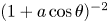 $(1 + a \cos \theta )^{-2}$ was added to inhibit the development of the
 $n = 0$ harmonic. The initial amplitudes for the modes
 $V_{c;n}(t)$ and
 $V_{s;n}(t)$ are
 \begin{equation} V_{c;n;0} = -\frac{V_0 \chi_{c;n}^2}{a\sqrt{2} (2+\chi_{c;n}^2)} {\mathcal{I}}_{c;n}, \quad V_{s;n;0} = \frac{V_0}{\sqrt{2}} {\mathcal{I}}_{s;n}, \end{equation}
where the notation  ${\mathcal {I}}_{*;n}$ (
 $* \in \{c,s\}$) was introduced in (4.14). The amplitudes
 $V_{c;n}(t)$ and
 $V_{s;n}(t)$ undergo exponential damping with their respective damping coefficients,
 $\nu \chi _{c;n}^2 / r^2$ and
 $\nu \chi _{s;n}^2 / r^2$, respectively. The general solution can be written as
 \begin{align} u^{\hat{\varphi}}(t,\theta) &= \frac{V_0}{\sqrt{2}}(1+a \cos\theta) \sum_{n = 1}^\infty \left[-\frac{\chi_{c;n}^2}{a(2+\chi_{c;n}^2)} {\mathcal{I}}_{c;n} \,\textrm{e}^{-\nu \chi_{c;n}^2 t / r^2} F_n(\theta) \right.\nonumber\\ &\qquad \qquad\qquad\qquad\qquad\left.\vphantom{\frac{\chi_{c;n}^2}{a(2+\chi_{c;n}^2)}}+ {\mathcal{I}}_{s;n} \,\textrm{e}^{-\nu \chi_{s;n}^2 t / r^2} G_n(\theta)\right]. \end{align}
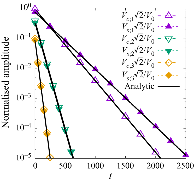
Figure 10 shows the time dependence of the amplitudes  $V_{c;n}(t)$ (dashed lines and empty symbols) and
 $V_{s;n}(t)$ (dotted lines and filled symbols) for
 $n = 1$ (purple upper triangles),
 $2$ (green lower triangles) and
 $3$ (orange rhombi). As expected from figure 8,
 $V_{c;1}(t)$ decays at a faster rate than
 $V_{s;1}(t)$. However, at
 $a = 0.4$, the eigenvalues
 $\chi _{c;n}$ and
 $\chi _{s;n}$ have roughly the same values when
 $n \ge 2$. Therefore, the decay rates of
 $V_{c;2}(t)$ and
 $V_{c;3}(t)$ are very similar to those of
 $V_{s;2}(t)$ and
 $V_{s;3}(t)$, respectively. In this benchmark test, the fluid and simulation parameters are the same as those employed in § 4.2.
Time evolution of the amplitudes  $V_{c;n}(t)$ (dashed lines and empty symbols) and
 $V_{s;n}(t)$ (dotted lines and filled symbols) for
 $n = 1$ (upper purple triangles),
 $2$ (lower green triangles) and
 $3$ (orange rhombi) on the torus with
 $a = 0.4$. The analytic prediction, (4.17), is shown with solid lines.

5. Viscous fluid: sound wave damping
In the previous sections, we considered the propagation of sound waves in the perfect fluid and the equivalent of shear wave damping in a viscous fluid. This section presents an analysis of the damping of longitudinal waves propagating along the poloidal direction through a viscous fluid. For simplicity, we assume that the fluid velocity along the azimuthal direction vanishes.
This section is structured as follows. The general solution for the damping of longitudinal waves propagating along the poloidal direction is presented in § 5.1. Then, a benchmark test is proposed in § 5.2.
5.1. General solution
The starting point of the analysis in this section is the Cauchy equation in the poloidal direction, (2.41b), which can be linearised as follows:
 \begin{align} \frac{\partial u^{\hat{\theta}}}{\partial t} + \frac{P_0}{\rho_0 r}\frac{\partial \delta P}{\partial \theta} & = \frac{\kappa \phi_0}{\rho_0 r^3} \frac{\partial}{\partial \theta} \left\{\frac{\partial_\theta[(1 + a \cos\theta)\partial_\theta \delta\phi]} {1 + a \cos\theta}\right\} \nonumber\\ &\quad + \frac{\nu}{r^2(1+a \cos\theta)^2} \frac{\partial}{\partial\theta} \left[(1 + a \cos\theta)^3 \frac{\partial}{\partial\theta}\left( \frac{u^{{\hat{\theta}}}}{1 + a \cos\theta}\right) \right]\nonumber\\ &\quad + \frac{\nu_{v}}{r^2} \frac{\partial}{\partial \theta} \left\{\frac{\partial_\theta[u^{\hat{\theta}}(1 + a \cos\theta)]} {1 + a \cos\theta}\right\}. \end{align}
The left-hand side of the above equation is similar to that encountered in the inviscid case, in (3.4). On the right-hand side, one can see that the differential operator with respect to  $\theta$ acting on
 $(1+ a\cos \theta )\partial _\theta \delta \phi$ and in the term proportional to
 $\nu _v$ is the one encountered in the inviscid case, defined in (3.10). In the term proportional to
 $\nu$, one can recognise the operator encountered in the damping of the shear wave problem, presented in (4.4). In principle, the normal modes analysis must be made with respect to the complete set of eigenfunctions and eigenvalues of only one operator. The set of eigenfunctions
 $\{\, f_n, g_n\}$ of the inviscid operator differs in general from the set
 $\{F_n, G_n\}$ corresponding to the viscous operator (they coincide only in the limit when
 $a \rightarrow 0$). Since the dominant phenomenon in the present set-up is the wave propagation, it is natural to work with the basis given by the inviscid operator and to treat the viscous operator as a perturbative effect. To this end, we take advantage of the identity
 \begin{align} & \frac{1}{(1+a \cos\theta)^2} \frac{\partial}{\partial\theta} \left[(1 + a \cos\theta)^3 \frac{\partial}{\partial\theta}\left( \frac{u^{{\hat{\theta}}}}{1 + a \cos\theta}\right) \right] \nonumber\\ &\quad = \frac{\partial}{\partial \theta} \left\{\frac{\partial_\theta[u^{\hat{\theta}}(1 + a \cos\theta)]} {1 + a \cos\theta}\right\} + \frac{2a \cos\theta}{1 + a \cos\theta} u^{\hat{\theta}}, \end{align}
which allows (5.1) to be written as
 \begin{align} \frac{\partial u^{\hat{\theta}}}{\partial t} + \frac{P_0}{\rho_0 r}\partial_\theta \delta P & = \frac{\kappa \phi_0}{\rho_0 r^3} \frac{\partial}{\partial \theta} \left\{\frac{\partial_\theta[(1 + a \cos\theta)\partial_\theta \delta\phi]} {1 + a \cos\theta}\right\} \nonumber\\ &\quad + \frac{\nu +\nu_{v}}{r^2} \partial_\theta \left\{\frac{\partial_\theta[u^{\hat{\theta}}(1 + a \cos\theta)]} {1 + a \cos\theta}\right\} + \frac{\nu}{r^2} \frac{2a \cos\theta}{1 + a \cos\theta} u^{\hat{\theta}}. \end{align}
In principle, as was the case for the inviscid fluid, the sound wave equation can be obtained by taking the time derivative of (5.3). However, this approach is not insightful. Instead, starting from (3.2), the time derivative of the pressure deviation can be replaced using the continuity, energy and Cahn–Hilliard equations, reproduced below in the linearised limit
 \begin{equation} \left.\begin{array}{c@{}} \displaystyle \dfrac{\partial \delta \rho}{\partial t} + \dfrac{\partial_\theta {\mathcal{U}}} {r(1 + a \cos\theta)} = 0,\\[12pt] \displaystyle \dfrac{\partial \delta e}{\partial t} + \dfrac{P_0}{\rho_0 e_0} \dfrac{\partial_\theta{\mathcal{U}}}{r(1 + a \cos\theta)} = \dfrac{k_0}{\rho_0 c_v} \dfrac{\partial_\theta[(1 + a \cos\theta) \partial_\theta \delta e]} {r^2(1 + a\cos\theta)}, \\[12pt] \displaystyle \dfrac{\partial \delta \phi}{\partial t} + \phi_0 \dfrac{\partial_\theta {\mathcal{U}}} {r(1 + a \cos\theta)} = \dfrac{M}{r^2} \dfrac{\partial_\theta[(1 + a\cos\theta)\partial_\theta \delta \mu]} {1 + a \cos\theta}. \end{array}\right\} \end{equation}
We remind the readers that we consider small perturbations around a stationary, background state, which we denote by the subscript 0. We also introduced the notation  ${\mathcal {U}} = u^{\hat {\theta }} (1 + a \cos \theta )$ and the deviation of the chemical potential from the background state
 $\delta \mu = \mu (\phi ) - \mu (\phi _0)$ is given by
 \begin{equation} \delta \mu = -A (1 - 3\phi_0^2) \delta \phi - \frac{\kappa}{r^2} \frac{\partial_\theta[(1 + a \cos\theta) \partial_\theta \delta \phi]} {1 + a \cos\theta}. \end{equation}
To solve the partial differential equations in (5.4), we seek normal solutions defined with respect to the complete set of modes  $\{\, f_n, g_n\}$ introduced in § 3. We introduce the following expansions:
 \begin{equation} \begin{pmatrix} u^{\hat{\theta}} & \partial_\theta \delta \rho & \partial_\theta \delta e\\ \partial_\theta \delta \phi & \partial_\theta \delta \mu & \partial_\theta \delta P \end{pmatrix} = \sum_{n = 0}^\infty\frac{ f_n(\theta)}{1 + a \cos\theta} \begin{pmatrix} U_{c;n} & R_{c;n} & E_{c;n}\\ \Phi_{c;n} & M_{c;n} & P_{c;n} \end{pmatrix}, \end{equation}
where for simplicity we assume that the flow parameters are even with respect to  $\theta$, such that the coefficients of the odd eigenfunctions
 $g_n(\theta )$ vanish. The amplitudes
 ${\mathcal {A}}_{c;n}(t)$ (
 ${\mathcal {A}} \in \{U, R, E, \Phi , M, P\}$) have the following time dependence:
 \begin{equation} {\mathcal{A}}_{c;n}(t) = {\mathcal{A}}_{c;n;0} \,\textrm{e}^{-\alpha_{c;n} t}. \end{equation}
The real part of  $\alpha _{c;n}$ controls the damping of the corresponding mode, while its imaginary part is responsible for its propagation. The extension to the case of odd or general flow configurations is straightforward, but will not be discussed here for brevity.
In order to find the normal frequencies  $\alpha _{c;n}$, we multiply (5.3) by
 $f_n(\theta )$ and integrate it with respect to
 $\theta$ between
 $0$ and
 $2{\rm \pi}$. We obtain
 \begin{align} -\alpha_{c;n} U_{c;n;0} + \frac{P_0}{\rho_0 r} P_{c;n;0} &= -\frac{\kappa \phi_0 \lambda_{c;n}^2}{\rho_0 r^3} \Phi_{c;n;0} - \frac{\nu+\nu_v}{r^2} \lambda_{c;n}^2 U_{c;n;0}\nonumber\\ &\quad - \frac{2\nu}{r^2} \sum_{\ell = 0}^\infty {\boldsymbol{\mathsf{M}}}_{n,\ell} U_{c;\ell;0}, \end{align}
where  $\lambda _{c;n}^2$ is defined in (3.15). The infinite matrix
 ${\boldsymbol{\mathsf{M}}}$ mixes the normal modes due to the last term in (5.3). Its components can be obtained as
 \begin{align} {\boldsymbol{\mathsf{M}}}_{n,\ell} &= -\int \frac{\textrm{d}\theta}{2{\rm \pi}} \frac{a \cos\theta }{(1 + a\cos\theta)^2} f_n(\theta) f_\ell(\theta)\nonumber\\ &= \int \frac{\textrm{d}\theta}{2{\rm \pi}} \left[\frac{1}{(1 + a \cos\theta)^2} - \frac{1}{1 + a\cos\theta}\right] f_n(\theta) f_\ell(\theta). \end{align}
In the case  $n = \ell = 0$, we find an analytic result
 \begin{equation} {\boldsymbol{\mathsf{M}}}_{0,0} = \frac{a^2}{1 - a^2}.\end{equation}
When  $\ell = 0$ and
 $n > 0$, the second term in the square brackets in (5.9) does not contribute due to the orthogonality relation given in (3.11). Comparing the first term with the definition of
 $I_{m;n}$ in (3.26) for
 $m = 2$ and noting that
 $f_0(\theta ) = (1-a^2)^{1/4}$ is a constant,
 ${\boldsymbol{\mathsf{M}}}_{n,0}$ can be written as
 \begin{equation} {\boldsymbol{\mathsf{M}}}_{n,0} = (1 - a^2)^{1/4} I_{c;2;n} - \delta_{n,0}.\end{equation}
The integral  $I_{c;2;n}$ (
 $n > 0$) can be obtained in terms of
 $I_{c;0;n}$ by integrating (3.15) with respect to
 $\theta$ and using integration by parts
 \begin{align} I_{c;0;n} &= -\frac{1}{\lambda_{c;n}^2} \int_0^{2{\rm \pi}} \frac{\textrm{d}\theta}{2{\rm \pi}} (1 + a \cos\theta) \frac{\textrm{d}}{\textrm{d}\theta} \left(\frac{\textrm{d}f_n / \textrm{d}\theta}{1 + a \cos\theta}\right)\nonumber\\ &= \frac{1}{\lambda_{c;n}^2} \int_0^{2{\rm \pi}} \frac{\textrm{d}\theta}{2{\rm \pi}} f_n(\theta) \left[\frac{1}{1 + a\cos\theta} - \frac{1 - a^2}{(1 + a\cos\theta)^2}\right]. \end{align}
The first term in the square brackets on the last line of the above equation vanishes for  $n > 0$. Setting
 $m =2$ in (3.26), it can be seen that the second term can be expressed in terms of
 $I_{c;2;n}$, such that the following relation can be established:
 \begin{equation} I_{c;2;n} = -\frac{\lambda_{c;n}^2}{1 - a^2} I_{c;0;n} + \frac{\delta_{n,0}}{(1 - a^2)^{5/4}}. \end{equation}
Putting together (5.10), (5.11) and (5.13) allows  $\boldsymbol{\mathsf{M}}_{n,0}$ to be expressed in the following form:
 \begin{equation} \boldsymbol{\mathsf{M}}_{n,0} = \frac{\delta_{n,0} a^2}{1 - a^2} -\frac{\lambda_{c;n}^2}{(1 - a^2)^{3/4}} I_{0;n}, \end{equation}
which is also valid at  $n= 0$ since the second term does not contribute due to the fact that
 $\lambda _{c;0} = 0$. Later in this section, the diagonal elements
 $\boldsymbol{\mathsf{M}}_{n,n}\text{ with }1\leq n\leq 3$ will be necessary for the computation of the acoustic damping coefficient. Their analytic approximations up to
 $O(a^9)$ are given in SM:3.3i of the supplementary material.
The next step is to find expressions for the quantities  $P_{c;n;0}$ and
 $\Phi _{c;n;0}$ in (5.8). To this end, we insert the decompositions in (5.6) into (5.4) and find
 \begin{equation} \left.\begin{array}{c@{}}
\displaystyle R_{c;n;0} =
-\dfrac{\lambda_{c;n}^2}{\alpha_{c;n} r} U_{c;n;0},\\
\displaystyle E_{c;n;0} = -\dfrac{P_0}{\rho_0 e_0}
\dfrac{\lambda_{c;n}^2}{\alpha_{c;n} r}
\dfrac{U_{c;n;0}}{\widetilde{E}_{c;n;0}},\\
\displaystyle M_{c;n;0} = \left[\dfrac{\lambda_{c;n}^2
\kappa}{r^2} - A(1 - 3\phi_0^2)\right]
\Phi_{c;n;0},\\
\displaystyle \Phi_{c;n;0} = -\phi_0
\dfrac{\lambda_{c;n}^2}{\alpha_{c;n} r}
\dfrac{U_{c;n;0}}{\widetilde{\Phi}_{c;n;0}},
\end{array}\right\} \end{equation}
where we introduced the following dimensionless quantities:
 \begin{equation} \widetilde{E}_{c;n;0} = 1 - \frac{\gamma \nu \lambda_{c;n}^2} {Pr\, r^2 \alpha_{c;n}}, \quad \widetilde{\Phi}_{c;n;0} = 1 + \frac{M \lambda_{c;n}^2}{r^2 \alpha_{c;n}} \left[A(1 - 3\phi_0^2) - \frac{\kappa \lambda_{c;n}^2}{r^2}\right]. \end{equation}
The pressure amplitude  $P_{c;n;0}$ can be obtained by combining the above results in conjunction with (3.2) via
 \begin{align} P_{c;n;0} &= \frac{\rho_0 P_{\rho,0}}{P_0} R_{c;n;0} + \frac{e_0 P_{e,0}}{P_0} E_{c;n;0} + \frac{P_{\phi,0}}{P_0} \Phi_{c;n;0}\nonumber\\ &= - \frac{\lambda_{c;n}^2 U_{c;n;0}}{\alpha_{c;n} r} \widetilde{P}_{c;n;0}. \end{align}
The dimensionless quantity  $\widetilde {P}_{c;n;0}$ was introduced for notational brevity, being given by
 \begin{equation} \widetilde{P}_{c;n;0} = \frac{\rho_0 P_{\rho,0}}{P_0} + \frac{P_{e,0}}{\rho_0 \widetilde{E}_{c;n;0}} + \frac{\phi_0 P_{\phi,0}}{P_0 \widetilde{\Phi}_{c;n;0}}. \end{equation}
Using the expression for  $P_{c;n;0}$ given in (5.17), (5.8) can be rearranged as a matrix equation
 \begin{equation} \boldsymbol{\mathsf{AU}} = 0,\end{equation}
where the column vector  $\boldsymbol{\mathsf{U}}$ has elements
 $\boldsymbol{\mathsf{U}}_n = U_{c;n;0}$, while the (infinite-dimensional) matrix
 $\boldsymbol{\mathsf{A}}$ has the following components:
 \begin{align} \boldsymbol{\mathsf{A}}_{n,m} = -\frac{\delta_{n,m}}{\alpha_{c;n}} \left[\alpha_{c;n}^2 + \frac{\lambda_{c;n}^2 P_0}{r^2 \rho_0} \widetilde{P}_{c;n;0} + \frac{\kappa \lambda_{c;n}^4 \phi_0^2}{\rho_0 r^4 \widetilde{\Phi}_{c;n;0}} - \frac{\alpha_{c;n}\lambda_{c;n}^2}{r^2} (\nu + \nu_{v})\right] + \frac{2\nu}{r^2} \boldsymbol{\mathsf{M}}_{n,m}. \end{align}
Equation (5.19) has non-trivial solutions when the determinant of the matrix  $\boldsymbol{\mathsf{A}}$ vanishes. This condition selects a discrete set of values for the coefficients
 $\alpha _{c;n}$. In order to find these values, we make the assumption that the dissipative terms are small on their respective dimensional scale, i.e.
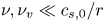 $\nu , \nu _{v} \ll c_{s,0} / r$,
 $\kappa \ll r^2$,
 $M \ll r c_{s,0}$. To this end, we introduce the small parameter
 $\varepsilon$, which allows us to write
 \begin{equation} \nu = \varepsilon \bar{\nu}, \quad \nu_{v} = \varepsilon \bar{\nu}_{v}, \quad \kappa = \varepsilon \bar{\kappa}, \quad M = \varepsilon \bar{M}. \end{equation}
We keep terms up to first order in  $\varepsilon$ for the rest of the section. We further assume that
 $\alpha _{c;n}$ can be written as
 \begin{equation} \alpha_{c;n} = \pm \textrm{i} \omega_{c;n} + \varepsilon \bar{\alpha}_{c;n;d}, \end{equation}
where  $\omega _{c;n}$ is the angular velocity and
 $\alpha _{c;n;d} = \varepsilon \bar{\alpha}_{c;n;d}$ is the damping factor.
It can be seen that the off-diagonal elements of the matrix  $\boldsymbol{\mathsf{A}}$ are at least one order higher with respect to
 $\varepsilon$ than the diagonal elements, being proportional to
 $\varepsilon \overline {\nu }$. When computing the determinant, the leading order contribution comes from the diagonal elements, while any off-diagonal contribution comes with an
 $O(\varepsilon ^2)$ penalty, such that
 \begin{equation} \det{\boldsymbol{\mathsf{A}}} = \boldsymbol{\mathsf{A}}_{11} \times \boldsymbol{\mathsf{A}}_{22} \times \boldsymbol{\mathsf{A}}_{33} \times \cdots + O(\varepsilon^2). \end{equation}
Thus, up to first order in  $\varepsilon$, the eigenvalues
 $\alpha _{c;n}$ can be found by requiring that each diagonal element
 $\boldsymbol{\mathsf{A}}_{nn}$ vanishes. We further note that there are typically multiple solutions stemming from
 $\boldsymbol{\mathsf{A}}_{nn} = 0$. The acoustic modes correspond to complex solutions for
 $\alpha _{c;n}$, allowing the corresponding modes to propagate. There are also real solutions for
 $\alpha _{c;n}$, such that the respective modes decay exponentially. In the case of the ideal thermal fluid, there is only one such solution, corresponding to the thermal mode. There is also one such mode corresponding to the Cahn–Hilliard equation, which we will refer to as the Cahn–Hilliard mode. For simplicity, when we use the Cahn–Hilliard equation, we assume that the fluid is isothermal.
We now discuss the  $n = 0$ mode, corresponding to the incompressible velocity profile. Since
 $\lambda _{c;0} = 0$, the case
 $n = 0$ is degenerate. There is only one eigenvalue corresponding to this case, which is given by
 \begin{equation} \alpha_{c;0} = \frac{2\nu}{R^2 - r^2},\end{equation}
where the relation  $\boldsymbol{\mathsf{M}}_{0,0} = a^2 / (1 - a^2) = r^2 / (R^2 - r^2)$ was employed. There is no imaginary part to
 $\alpha _{c;0}$, showing that the mode corresponding to the incompressible velocity profile does not propagate. Furthermore, since
 $\alpha _{c;0} > 0$, the amplitude of this mode decays exponentially through viscous damping. On the flat geometry, the incompressible one-dimensional flow corresponds to a constant velocity, which cannot suffer viscous damping due to the Galilean invariance of the theory. In contrast, on the torus, Galilean invariance is no longer valid. While the inviscid fluid supports (in the linearised regime) the incompressible flow profile as an exact, time-independent solution, this zeroth-order mode with respect to the set
 $\{\, f_n, g_n\}$ is no longer preserved in the case of the viscous fluid, since
 $f_0 (1 + a \cos \theta )$ does not provide an eigenfunction of the viscous operator in (4.4). The damping of the zeroth-order mode, given in (5.24), depends only on the kinematic viscosity and seems to be independent of the type of fluid considered. Thus,
 $\alpha _{c;0}^{-1}$ provides a fundamental time scale on which, in the absence of external forcing, the flow on the poloidal direction becomes quiescent.
For  $n > 0$, the angular frequency
 $\omega _{c;n}$ for the acoustic mode is given by
 \begin{equation} \omega_{c;n} = \frac{\lambda_{c;n} c_{s;\kappa;c;n}}{r},\quad c_{s;\kappa;c;n}^2 = c_{s;0}^2 + \frac{\kappa \lambda_{c;n}^2}{\rho_0 r^2} \phi_0. \end{equation}
The acoustic damping coefficient  $\alpha _{c; n; a} = \varepsilon \bar{\alpha}_{c;n;a}$ (as a shorthand, we remove the subscript
 $d$ and add a subscript
 $a$ to describe the acoustic damping coefficient) receives contributions from the viscous terms, as well as from the energy and Cahn–Hilliard terms
 \begin{equation} \alpha_{c;n; a} = \frac{\nu}{r^2} \boldsymbol{\mathsf{M}}_{n,n} + \frac{\lambda_{c;n}^2}{2r^2} \left[\nu \left(1 + \frac{\gamma P_0 P_{e,0}}{\rho_0^2 c_{s;\kappa;c;n}^2 Pr} \right) + \nu_{v} - \frac{M \phi_0 P_{\phi,0}} {\rho_0 c_{s;\kappa;c;n}^2} A(1 - 3\phi_0^2)\right]. \end{equation}
We remind the reader that  $\alpha _{c;n;a}$ together with the angular frequency
 $\omega _{c;n}$ make up the acoustic mode,
 $\alpha _{c;n} \rightarrow \alpha _{c;n;a} \pm \textrm {i} \omega _{c;n}$. We note that (5.25) and (5.26) are valid for all types of fluids considered in this paper, namely: the ideal isothermal fluid, the ideal thermal fluid and the isothermal fluid coupled with the Cahn–Hilliard equation.
The thermal and Cahn–Hilliard modes can be obtained by setting, in (5.20),  $\alpha _{c;n}$ to
 $\varepsilon \bar {\alpha }_{c;n;t}$ or
 $\varepsilon \bar {\alpha }_{c;n;\phi }$, respectively, while setting the angular frequency
 $\omega _{c;n} = 0$. The values of
 $\alpha _{c;n}$ satisfying the above ansatz are found by solving the following equation:
 \begin{equation} \widetilde{P}_{c;n;0} = 0, \end{equation}
which is quadratic in  $\alpha _{c;n}$. In the general case of the thermal flow of a non-ideal (Cahn–Hilliard) fluid, the solution of this equation is too lengthy to be reproduced here. In the next section we will specialise the equation to the fluid types introduced in § 3, namely an ideal isothermal fluid, an ideal fluid with variable temperature and an isothermal multicomponent fluid coupled with the Cahn–Hilliard equation, allowing for simple expressions to be obtained. These solutions are presented in (5.36), (5.37) and (5.38), respectively.
5.2. Benchmark test
We now focus on a specific example. At initial time,  $t=0$, we assume that the density, internal energy and order parameter fields are unperturbed, while the velocity profile is that of the incompressible fluid
 \begin{equation}\delta \rho_0 = 0, \quad \delta e_0 = 0, \quad \delta \phi_0 = 0, \quad u^{\hat{\theta}}_0 = \frac{U_0}{1 + a \cos\theta}. \end{equation}
The analysis of the normal modes was performed in the limit where the modes become fully decoupled (the non-diagonal elements of the matrix  $\boldsymbol{\mathsf{M}}$ were ignored). For the particular case considered here, we are also interested in finding the time dependence of the amplitudes
 $U_{c;n}(t)$, defined through (5.6). To do this, it is sufficient to employ the initial conditions in (5.28) in order to find the full solution. From (5.28) and (5.3), it can be seen that
 \begin{equation} U_{c;n}(0) = \frac{U_0 \delta_{n,0}}{(1 -a^2)^{1/4}}, \quad \dot{U}_{c;n}(0) = -\frac{2\nu U_0}{r^2 (1 - a^2)^{1/4}} \boldsymbol{\mathsf{M}}_{n,0}. \end{equation}
The time dependence of the amplitude of the  $n= 0$ mode is
 \begin{equation} U_{c;0}(t) = \frac{U_0}{(1 - a^2)^{1/4}} \,\textrm{e}^{-2\alpha_\nu t}, \quad \alpha_\nu \equiv \frac{1}{2} \alpha_{c;0} = \frac{\nu}{R^2 - r^2}, \end{equation}
where  $\alpha _\nu$ is the principal damping coefficient which will be fundamental for discussing the dynamics of the stripe configurations in § 7.
For the higher-order harmonics, and when the temperature or Cahn–Hilliard equation is taken into account, a third equation is required to fix the integration constant for the thermal or Cahn–Hilliard mode. This can be obtained by taking the time derivative of (5.3), yielding
 \begin{equation} \ddot{U}_{c;n} + \frac{P_0}{\rho_0 r} \dot{P}_{c;n} + \frac{\kappa \lambda_{c;n}^2 \phi_0}{r^3} \dot{\Phi}_{c;n} + \frac{\nu + \nu_{v}}{r^2} \lambda_{c;n}^2 \dot{U}_{c;n} + \frac{2\nu}{r^2} \sum_{m = 0}^\infty \boldsymbol{\mathsf{M}}_{n,m} \dot{U}_{c;m} = 0. \end{equation}
The time derivative  $\dot {P}_{c;n}$ can be obtained in analogy to (5.17), by differentiating (3.2) with respect to
 $\theta$ and
 $t$, multiplying it by
 $f_n(\theta )$ and then integrating it with respect to
 $\theta$
 \begin{equation} \dot{P}_{c;n} = \frac{\rho_0 P_{\rho,0}}{P_0} \dot{R}_{c;n} + \frac{e_0 P_{e,0}}{P_0} \dot{E}_{c;n} + \frac{P_{\phi,0}}{P_0} \dot{\Phi}_{c;n}.\end{equation}
The time derivatives  $\dot {R}_{c;n}$,
 $\dot {E}_{c;n}$ and
 $\dot {\Phi }_{c;n}$ can be obtained by differentiating all three relations in (5.4) with respect to
 $\theta$, multiplying them by
 $f_n(\theta )$ and integrating them with respect to
 $\theta$. Noting that, at initial time, the perturbations
 $\delta e$,
 $\delta \rho$ and
 $\delta \phi$ vanish, the right-hand sides of the relations in (5.4) cancel, such that the following results are obtained:
 \begin{equation} \begin{pmatrix} \dot{R}_{c;n}(0)\\ \dot{E}_{c;n}(0)\\ \dot{\Phi}_{c;n}(0) \end{pmatrix} = \frac{\lambda_{c;n}^2}{r} \frac{\delta_{n,0} U_0}{(1- a^2)^{1/4}} \begin{pmatrix} 1 \\ P_0 / \rho_0 e_0 \\ \phi_0 \end{pmatrix} = \begin{pmatrix} 0 \\ 0 \\ 0 \end{pmatrix}. \end{equation}
The latter equality follows after taking into account that  $\lambda _{c;0} = 0$. Substituting the above results in (5.32), it can be seen that
 $\dot {P}_{c;n}(0) = 0$. Since
 $\dot {\Phi }_{c;n}(0)$ also cancels by virtue of (5.33), the second and third terms in (5.31) can be dropped. The fourth and fifth terms in (5.31) are of second order with respect to the damping coefficients
 $\nu$ and
 $\nu _v$, and thus of order
 $O(\varepsilon ^2)$ in the language of (5.21). For consistency, we approximate
 $\ddot {U}_{c;n}(0) = O(\varepsilon ^2) \simeq 0$. Thus, the solution which is accurate to first order in
 $\varepsilon$ is
 \begin{equation} U_{c;n}(t) = \frac{2\nu U_0 \lambda_{c;n}^2}{\omega_{c;n} r^2} \frac{I_{c;0;n}}{1 - a^2} \sin(\omega_{c;n}t)\,\textrm{e}^{-\alpha_{c;n;a} t}, \quad \forall n > 0. \end{equation}
The above solution was obtained under general considerations and therefore it applies to all types of fluids studied in this paper. The full solution can be constructed via the expansion in (5.6)
 \begin{equation} u^{\hat{\theta}}(t,\theta) = \frac{1}{1 + a\cos\theta} \sum_{n = 0}^\infty U_{c;n}(t) f_n(\theta). \end{equation}
In the following, we give a set of tests for the ideal isothermal fluid, the ideal fluid with variable temperature and the isothermal multicomponent fluid. The initial velocity amplitude is set to  $U_0 = 10^{-5}$.
For the isothermal ideal fluid, (5.25) and (5.26) reduce to
 \begin{equation} \left.\begin{array}{c@{}} \displaystyle c_{s,\kappa;c;n}^2 = c_{s,0}^2 = \dfrac{k_B T_0}{m},\\[12pt] \displaystyle \alpha_{c;n;a} = \dfrac{\nu}{r^2} \boldsymbol{\mathsf{M}}_{n,n} + \dfrac{\lambda_{c;n}^2(\nu + \nu_v)}{2r^2}. \end{array}\right\} \end{equation}
We set the background density and temperature to  $\rho _0 = 1$ and
 $T_0 = 1$, respectively, and take units such that
 $c_{s,0} = 1$. The kinematic viscosity is set to
 $\nu = 0.01$ and we consider two test cases, corresponding to
 $\nu _{v} = 0$ and
 $0.02$.
In the case of the variable temperature ideal fluid, (5.25) and (5.26) reduce to
 \begin{equation} \left.\begin{array}{c@{}} \displaystyle c_{s,\kappa;c;n}^2 = c_{s,0}^2 = \dfrac{\gamma K_B T_0}{m},\\[12pt] \displaystyle \alpha_{c;n;a} = \dfrac{\nu}{r^2} \boldsymbol{\mathsf{M}}_{n,n} + \dfrac{\lambda_{c;n}^2}{2r^2} \left[\nu\left(1 + \dfrac{\gamma - 1}{Pr} \right) +\nu_{v}\right],\\[12pt] \displaystyle \alpha_{c;n;t} = \dfrac{\lambda_{c;n}^2 \nu} {r^2 Pr}. \end{array}\right\} \end{equation}
We consider the case when  $c_v = k_B / m$, such that
 $\gamma = 2$. In order to match the sound speed of the isothermal fluid (
 $c_{s,0} = 1$), the background temperature is set to
 $T_0 = 0.5$. The background density is also kept at
 $\rho _0 = 1$. We further consider the case when the Prandtl number is
 $Pr = 2/3$, such that
 $k_0 = 3\nu$. In order to ensure that
 $\alpha _{c;n;a}$ matches the value corresponding to the isothermal case, the kinematic viscosity is set to
 $\nu = 0.004$, such that
 $k_0 = 0.012$. As before, we consider two values for the bulk kinematic viscosity, namely
 $\nu _{v} = 0$ and
 $0.02$.
In the case of the isothermal multicomponent fluid, (5.25) and (5.26) reduce to
 \begin{equation} \left.\begin{array}{c@{}} \displaystyle c_{s,\kappa;c;n}^2 = c_s^2 + \dfrac{\kappa\lambda_{c;n}^2}{\rho_0 r^2} \phi_0^2 = \dfrac{k_B T_0}{m} - \dfrac{\phi_0^2}{\rho_0}\left[A (1 - 3\phi_0^2) - \displaystyle \dfrac{\kappa\lambda_{c;n}^2}{r^2}\right],\\[12pt] \alpha_{c;n;a} = \dfrac{\nu}{r^2} \boldsymbol{\mathsf{M}}_{n,n} + \dfrac{\lambda_{c;n}^2}{2r^2} \left[\nu + \nu_{v} + \dfrac{M A^2}{\rho_0 c_{s;\kappa;c;n}^2} \phi_0^2(1 - 3\phi_0^2)^2 \right],\\[12pt] \displaystyle \alpha_{c;n;\phi} = \dfrac{M P_{\rho,0} \lambda_{c;n}^2}{r^2 c_{s,0}^2} A(3\phi_0^2 - 1) = \dfrac{M \lambda_{c;n}^2}{r^2} \dfrac{k_B T_0}{m c_{s,0}^2} A(3\phi_0^2 - 1). \end{array}\right\} \end{equation}
It can be seen that within the spinodal region, where 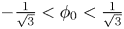 $-\frac {1}{\sqrt {3}} < \phi _0 < \frac {1}{\sqrt {3}}$,
 $\alpha _{c;n;\phi } < 0$ and spontaneous domain decomposition can occur through an exponential growth of fluctuations. We thus conduct the simulations outside this region, namely for the background value
 $\phi _0 = 0.8$ of the order parameter. Keeping the density at
 $\rho _0 = 1$, the interaction strength
 $A = 1$ and the surface tension parameter
 $\kappa = 5 \times 10^{-4}$, the temperature required to match the isothermal sound speed
 $c_{s;\kappa;c;n} = 1$ is
 $T_0 \simeq 0.4112$ (this is true only for the zeroth-order mode, when
 $\lambda _{c;0} = 0$). We consider the case when the mobility parameter
 $M$ is equal to the kinematic viscosity. In order to obtain the same acoustic damping coefficients as in the isothermal case, we set
 $M = \nu \simeq 6.486 \times 10^{-3}$. As before,
 $\nu _v$ takes the values
 $0$ and
 $0.02$.
The parameter values discussed above are also summarised in table 4. The other quantities required to compute the solutions  $U_{c;n}$ (for
 $n > 0$), given in (5.34), are summarised in table 5.
Values for the background temperature  $T$, kinematic viscosity
 $\nu$ and principal damping coefficient
 $\alpha _\nu$ defined in (5.30), for the isothermal ideal fluid (Iso), variable temperature ideal fluid (Th) and isothermal multicomponent fluid (CH) on the torus with
 $a = 0.4$. The background density is in all cases
 $\rho = 1$. The heat conductivity and adiabatic index for the thermal model are
 $k = 0.012$ and
 $\gamma = 2$, corresponding to
 $Pr = 2/3$. The parameters for the multicomponent fluid are
 $M = \nu \simeq 6.486 \times 10^{-3}$,
 $A = 1$ and
 $\kappa = 5 \times 10^{-4}$. The parameters are chosen such that
 $c_s^2 = 1$.

Values of various parameters required to build the solution in (5.34) when  $a = 0.4$. The bulk kinematic viscosity
 $\nu _v$ required to compute the coefficient
 $\alpha _{c;n;a}$ in the last column is set to
 $\nu _v = 0.02$. The amplitudes are computed by dividing the prefactors in (5.34) by the initial velocity amplitude
 $U_0 = 10^{-5}$.

We now discuss the benchmark test results. In figure 11, we validate the analytic solution using numerical simulations for the  $2\times 3$ cases discussed above. The simulations were conducted using
 $N_\theta = 320$ nodes and a time step
 $\delta t = 5 \times 10^{-4}$ on the torus with
 $a = 0.4$. The amplitude of the
 $n = 0$ mode is shown in figure 11(a). As predicted by (5.30), the damping coefficient
 $2\alpha _\nu$ of
 $U_{c;0}$ depends only on the kinematic viscosity. This is natural since the bulk viscosity cannot affect the mode corresponding to the incompressible velocity profile. Thus, the results for
 $\nu _v = 0$ and
 $\nu _v = 0.02$ are overlapped and only three distinct curves can be seen in figure 11(a), corresponding to the differing values of the background kinematic viscosity
 $\nu$ employed in the three fluids discussed above (these values are summarised in table 4). The careful choice of parameters discussed above and summarised in table 4 ensures that the acoustic damping coefficients
 $\alpha _{c;n;a}$ corresponding to the higher-order modes have the same values. Thus, only two distinct curves can be seen in figure 11(b–d), corresponding to
 $\nu _{v} = 0$ (lesser damping, shown with dashed black lines and empty symbols) and to
 $\nu _{v} = 0.02$ (stronger damping, shown with dotted red lines and filled symbols). The results for the isothermal (Iso), variable temperature (Th) and multicomponent fluids (CH), shown with squares, circles and rhombi, are overlapped at fixed values of
 $\nu _v$. In all cases, the analytic predictions are shown with a continuous blue line and the agreement with the numerical results is excellent.
Time evolution of the ratio  $U_{c;n}(t)/U_0$ for the initial velocity profile given in (5.28), for (a)
 $n = 0$, (b)
 $n = 1$, (c)
 $n = 2$ and (d)
 $n = 3$, on the torus with
 $a = 0.4$. The simulation results for
 $\nu _v = 0$ are shown with dashed black lines and empty symbols, while those for
 $\nu _v = 0.02$ are shown with dotted red lines and filled symbols. The analytic predictions for
 $U_{c;0}$ (5.30) and
 $U_{c;n>0}$ (5.34) are shown with solid blue lines. The results corresponding to the variable temperature (Th), multicomponent (CH) and isothermal (Iso) fluids are shown using squares, circles and rhombi, respectively.

6. Stripe configurations in equilibrium: Laplace pressure test
This section starts the series of benchmark problems concerning an isothermal multicomponent fluid in axisymmetric ring-type configurations. We begin this section by discussing the properties of the equilibrium position in § 6.1. The stability of these equilibria with respect to non-axisymmetric configurations, as well as with respect to azimuthal perturbations, is addressed in § 6.2. The benchmark test proposed in § 6.3 concerns a generalisation of the Laplace–Young pressure law, giving the difference between the pressures measured inside and outside of the considered stripe configuration.
6.1. Equilibrium position
Let the stripe interfaces be located at
 \begin{equation} \theta_- = \theta_c - {\rm \Delta} \theta / 2, \quad \theta_+ = \theta_c + {\rm \Delta} \theta / 2, \end{equation}
where  ${\rm \Delta} \theta$ is the angular span of the stripe and
 $\theta _c$ is its centre. The remaining part of the fluid domain consists of a stripe of width
 $2{\rm \pi} - {\rm \Delta} \theta$, centred on
 $\theta _c + {\rm \pi}$, which is conjugate to the main stripe. For consistency, we only refer to the domain for which
 $0 < {\rm \Delta} \theta < {\rm \pi}$ as ‘the stripe’ in what follows. A snapshot of a typical stripe configuration on the torus is shown figure 12(a). The notation introduced above is highlighted in a
 $(\varphi ,\theta )$ plot in figure 12(b).
The axisymmetric stripe configurations: (a) torus view and (b)  $(\theta, \varphi)$ view. The colour maps the value of the order order parameter. The stripe is shown in dark colour.

Since the torus is not geometrically homogeneous with respect to the  $\theta$ direction, there will be preferred locations where the stripe can be in static equilibrium. These locations are found by imposing the minimisation of the total interface length subject to fixed stripe area
 ${\rm \Delta} A$, which is a universal requirement for all fluids where interfaces are present. The stripe area can be found by integrating over the domain spanned by the stripe
 \begin{equation} {\rm \Delta} A = 2{\rm \pi} r R \int_{\theta_-}^{\theta_+} \textrm{d}\theta (1 + a \cos\theta) = 2{\rm \pi} r R [{\rm \Delta} \theta + 2a \sin({\rm \Delta} \theta / 2) \cos \theta_c]. \end{equation}
On the other hand, the total interface length  $\ell _{\mathit {total}}$ can be found by adding the circumferences
 $\ell _+$ and
 $\ell _-$ corresponding to
 $\theta = \theta _+$ and
 $\theta = \theta _-$, respectively
 \begin{align} \ell_{\mathit{total}} &= \ell_+ + \ell_- = 2{\rm \pi} R (1 + a \cos \theta_+) + 2{\rm \pi} R (1 + a \cos\theta_-) \nonumber\\ &= 4{\rm \pi} R \left(1 + a \cos \frac{{\rm \Delta} \theta}{2} \cos\theta_c \right). \end{align}
It can be expected that the minimisation of the interface length is required in order for the free energy, (2.6), to reach a minimum. In § SM:2.3 of the supplementary material, we show that this is indeed the case to leading order with respect to  $\xi _0$. The correction is due to the fact that the interface shape profile, and hence the line tension, in principle have a weak dependence on the curvature of the surface.
In order to derive the equilibrium positions, we impose a fixed area  ${\rm \Delta} A$. Taking the differential of (6.2) gives
 \begin{equation} \textrm{d}{\rm \Delta} A = 4{\rm \pi} r R \left[\left(1 + a \cos \frac{{\rm \Delta} \theta}{2} \cos\theta_c \right) \textrm{d} \frac{{\rm \Delta} \theta}{2} - a \sin\frac{{\rm \Delta} \theta}{2} \sin\theta_c \,\textrm{d}\theta_c \right]. \end{equation}
Setting  $\textrm {d}{\rm \Delta} A = 0$ allows infinitesimal changes
 $\textrm {d}({\rm \Delta} \theta )$ in the stripe width to be expressed in terms of changes in the position of the stripe centre through
 \begin{equation} \textrm{d}\frac{{\rm \Delta} \theta}{2} = \dfrac{a \sin \dfrac{{\rm \Delta} \theta}{2} \sin \theta_c} {1 + a \cos\dfrac{{\rm \Delta}\theta}{2} \cos\theta_c } \,\textrm{d}\theta_c. \end{equation}
At equilibrium, the interface length  $\ell _{\mathit {total}}$ [(6.3)] is minimised. Mathematically, this implies
 \begin{equation} \textrm{d} \ell_{\mathit{total}} = -4{\rm \pi} r \left(\sin \frac{{\rm \Delta} \theta}{2} \cos\theta_c \,\textrm{d} \frac{{\rm \Delta} \theta}{2} + \cos\frac{{\rm \Delta} \theta}{2} \sin \theta_c \,\textrm{d}\theta_c\right) = 0. \end{equation}
Substituting (6.5) into (6.6) yields
 \begin{equation} \left(a \cos\theta_c + \cos\frac{{\rm \Delta} \theta}{2}\right) \sin\theta_c = 0, \end{equation}
where it is understood that  ${\rm \Delta} \theta$ and
 $\theta _c$ are measured when the stripe is already at its equilibrium position.
One possibility for (6.7) to be satisfied is when  $\sin \theta _c =0$. This corresponds to two potential solutions,
 $\theta _c = 0$ and
 $\theta _c = {\rm \pi}$. From (6.3), it can be seen that
 $\theta _c = 0$ corresponds to an unstable equilibrium for stripes with
 ${\rm \Delta} \theta < {\rm \pi}$. Conversely,
 $\theta _c = {\rm \pi}$ is unstable for the conjugate stripes, having
 ${\rm \Delta} \theta > {\rm \pi}$. Thus, for stripes with small areas, the minimum energy configuration is attained for
 \begin{equation} \theta^{eq}_{c} = {\rm \pi}. \end{equation}
We now argue that the above solution is not universally valid for all stripe widths. Since the conjugate stripe, having width  $2{\rm \pi} - {\rm \Delta} \theta$, does not equilibrate at
 $\theta _c^{eq} = {\rm \pi}$, it is clear that increasing the stripe area must change the equilibrium position from
 $\theta ^{eq}_c = {\rm \pi}$ towards
 $\theta ^{eq}_c = 0$ (or
 $2{\rm \pi}$). To illustrate this point, let us consider the case of a maximally wide stripe with
 ${\rm \Delta} \theta = {\rm \pi}$. In this case, the conjugate stripe also has width
 $2{\rm \pi} - {\rm \Delta} \theta = {\rm \pi}$, and should thus be obtained via a symmetry transformation from the initial stripe. The only symmetry of the torus geometry is
 $z \rightarrow -z$. Thus, it is clear that the stripe can sit either on the upper half of the torus (centred on
 $\theta _c^{eq} = {\rm \pi}/2$), or on its bottom half (where
 $\theta _c^{eq} = 3{\rm \pi} /2$). Both configurations are equally stable and it can be seen that (6.7) is satisfied because the expression between the parentheses vanishes, while the term
 $\sin \theta _c^{eq} = 1$ is non-vanishing.
We expect that the equilibrium positions at  $\theta _c^{eq} = {\rm \pi}$ for small stripes and at
 $\theta _c^{eq} = {\rm \pi}\pm {\rm \pi}/2$ are connected smoothly as the area is increased. Thus,
 $\theta _c^{eq}$ must detach from
 ${\rm \pi}$ when the equilibrium stripe width exceeds a critical value,
 ${\rm \Delta} \theta _{\mathit {crit}}$. We can deduce that this critical stripe width
 ${\rm \Delta} \theta _{\mathit {crit}}$ corresponds to the case where both terms in (6.7) vanish simultaneously, leading to
 \begin{equation} {\rm \Delta} \theta_{\mathit{crit}} = 2\arccos(a). \end{equation}
Substituting the above value into (6.2) yields a critical area,
 \begin{equation} {\rm \Delta} A_{\mathit{crit}} = 4{\rm \pi} r R (\arccos a - a\sqrt{1 - a^2}). \end{equation}
When  ${\rm \Delta} A > {\rm \Delta} A_{\mathit {crit}}$, the point
 $\theta _c = {\rm \pi}$ corresponds to a local maximum value for
 $\ell _{\mathit {total}}$. Instead the global minima correspond to the case where only the parenthesis in (6.7) goes to zero
 \begin{equation} \theta^{eq}_{c} = {\rm \pi}\pm \arccos\left[\frac{1}{a} \cos\frac{{\rm \Delta} \theta_{eq}}{2}\right], \end{equation}
where  ${\rm \Delta} \theta _{eq} \equiv {\rm \Delta} \theta (\theta _c^{eq})$ is the stripe width when it is located at the equilibrium position. We can further show that the total interface length when
 $\theta _c = \theta ^{eq}_{c}$ is
 \begin{equation} \ell_{\mathit{total}; \textit{min}} = 4{\rm \pi} R \sin^2 \frac{{\rm \Delta} \theta_{eq}}{2}, \end{equation}
with  ${\rm \Delta} \theta _{eq}$ satisfying
 \begin{equation} {\rm \Delta} \theta_{eq} - a \sin {\rm \Delta} \theta_{eq} = \frac{{\rm \Delta} A}{2{\rm \pi} r R} = \frac{2{\rm \Delta} A}{{\rm \Delta} A_{\mathit{crit}}} (\arccos a - a \sqrt{1 - a^2}). \end{equation}
To better understand the nature of the solutions of (6.7), figure 13 shows the total interface length  $\ell _{\mathit {total}}$ for various ratios of
 ${\rm \Delta} A / {\rm \Delta} A_{\mathit {crit}}$. For
 ${\rm \Delta} A / {\rm \Delta} A_{\mathit {crit}} < 1$, the global minimum configuration is unique and corresponds to
 $\theta ^{eq}_c = {\rm \pi}$. Then, as we increase
 ${\rm \Delta} A / {\rm \Delta} A_{\mathit {crit}}$ beyond 1, there is a second-order phase transition. The minimum energy configurations become bistable, as given in (6.11).
Interface length  $\ell _{\mathit {total}}$ on a torus with
 $a = 0.4$ for various ratios of
 ${\rm \Delta} A / {\rm \Delta} A_{\mathit {crit}}$. For
 ${\rm \Delta} A / {\rm \Delta} A_{\mathit {crit}} < 1$ the global minimum is located at
 $\theta _c = {\rm \pi}$, while for
 ${\rm \Delta} A / {\rm \Delta} A_{\mathit {crit}} > 1$ there are two equivalent minima, as given by (6.11).

6.2. Stability of stripe configurations
In this section, we consider a relaxation of the axial symmetry constraint in order to explore the viability of the stripe configurations discussed in the previous subsection in the context of two-dimensional flows. We first discuss the stability of the stripe configurations with respect to small perturbations. The main idea is to see the effects of increasing the amplitude of azimuthal interface perturbations at the level of orthogonal modes. Those modes whose growth causes the interface length to decrease lead to instability. Our analysis is limited to the linear growth regime.
Since the upper ( $\theta _+$) and lower
 $(\theta _-)$ interfaces are separated by the stripe domain, it is reasonable to neglect the back reaction caused by perturbing one interface on the shape of the other. For definiteness, we focus on the lower interface
 $\theta _-$ and assume that it is perturbed according to
 \begin{equation} \theta_-(\varphi) = \theta_{-;0} + \delta \theta_-(\varphi), \end{equation}
where  $\theta _{-;0}$ is the average value of
 $\theta _-(\varphi )$, while
 $\delta \theta _- (\varphi )$ is a small position-dependent fluctuation, which admits the following Fourier decomposition:
 \begin{equation} \delta \theta_-(\varphi) = \frac{\delta}{\rm \pi} \sum_{n = 1}^\infty A_n \cos (n \varphi + \varphi_{n;0}), \end{equation}
where  $\delta > 0$ is an overall positive infinitesimal factor, while the coefficients
 $A_n = O(1)$ are not necessarily small. We assume that
 $\theta _{-;0}$ changes under the perturbation such that the domain area,
 \begin{align} {\rm \Delta} A &= r R \int_0^{2{\rm \pi}} \textrm{d}\varphi \int_{\theta_-(\varphi)}^{\theta_+} \textrm{d}\theta\, (1 + a \cos\theta) \nonumber\\ &= 2{\rm \pi} r R \left[\theta_+ - \theta_{-;0} + a \sin\theta_+ - a \sin\theta_{-;0} \left(1 - \frac{\delta^2}{4{\rm \pi}^2} \sum_{n = 1}^\infty A_n^2\right) + O(\delta^3)\right], \end{align}
remains constant. Keeping in mind that the back reaction on  $\theta _+$ is negligible, imposing
 $\textrm {d} {\rm \Delta} A / \textrm {d}\delta = 0$ implies that
 \begin{equation} \frac{\textrm{d} \theta_{-;0}}{\textrm{d}\delta} = \frac{\delta}{2{\rm \pi}^2} \frac{a \sin\theta_{-;0}}{1 + a \cos\theta_{-;0}} \sum_{n = 1}^\infty A_n^2. \end{equation}
Let us now compute the length  $\ell _-$ of the lower interface
 \begin{align} \ell_- &= \int_{0}^{2{\rm \pi}} \textrm{d}\varphi \sqrt{R^2 [1 + a \cos \theta(\varphi)]^2 + r^2 \left(\frac{\textrm{d} \theta_-}{\textrm{d}\varphi}\right)^2}\nonumber\\ &= 2{\rm \pi} R(1 + a \cos\theta_{-;0}) + \frac{r \delta^2}{2{\rm \pi}} \sum_{n=1}^\infty \left( \frac{a n^2}{1 + a \cos\theta_{-;0}} - \cos\theta_{-;0}\right) A_n^2 + O(\delta^3). \end{align}
Taking the differential of  $\ell _-$ with respect to
 $\delta$ while imposing (6.17) yields
 \begin{equation} \frac{\textrm{d}\ell_-}{\textrm{d}\delta} = \frac{r \delta}{\rm \pi} \sum_{n = 1}^\infty \frac{a(n^2 - 1) - \cos\theta_{-;0}}{1 + a\cos\theta_{-;0}} A_n^2. \end{equation}
The first term in the numerator has a stabilising effect, acting only on the Fourier modes with  $n > 1$. The second term can be related to the Gaussian curvature
 $K$, given by
 \begin{equation} K \equiv K(\theta) = \frac{\cos\theta}{rR (1 + a \cos\theta)}. \end{equation}
The  $n = 1$ mode becomes unstable when
 $K > 0$ and
 $\ell _-$ decreases when
 $\delta$ is increased, i.e. in the region of the torus given by
 $-{{\rm \pi} }/{2} < \theta _{-;0} < {{\rm \pi} }/{2}$. The higher-order modes become unstable deeper in the region of positive
 $K$, i.e. when
 $\cos \theta_{-;0}$ exceeds
 $a(n^2 - 1)$. An equivalent analysis can be performed for the upper interface, located at
 $\theta _+ = \theta _c + {\rm \Delta} \theta / 2$. Focussing now only on the onset of instability due to the first mode, (6.19) can be written as
 \begin{equation} \left(\frac{\textrm{d}\ell_\pm}{\textrm{d}\delta}\right)_{n=1} = - \frac{r^2 R A_1^2 \delta}{\rm \pi} K(\theta_{\pm;0}). \end{equation}
Equation (6.21) indicates that the upper and lower interfaces can become unstable simultaneously only when the stripe is completely contained in the region where  $K > 0$ (i.e. on the outer side of the torus).
We now discuss the stability of stripes with equilibrium position characterised by (6.7), as derived in the previous subsection. Essentially, instability occurs when  $\theta _{-}^{eq} = \theta _c^{eq} - {{\rm \Delta} \theta _{eq}}/{2} < {{\rm \pi} }/{2}$ or
 $\theta _{+}^{eq} = \theta _c^{eq} + {{\rm \Delta} \theta _{eq}}/{2} > {3{\rm \pi} }/{2}$. The subcritical stripes (having
 ${\rm \Delta} A < {\rm \Delta} A_{\mathit {crit}}$, which stabilise at
 ${\rm \pi}$) do not suffer from the instability described by (6.21). For the critical stripe, as described by (6.9), it can be seen that the instability condition on both the upper and lower interfaces reduces to
 $\textrm {arccos}\, a > {{\rm \pi} }/{2}$, which is marginally satisfied only in the case
 $a \rightarrow 0$. Next, supercritical stripes (having
 ${\rm \Delta} A > {\rm \Delta} A_{\mathit {crit}}$, which stabilise away from
 ${\rm \pi}$) are stable only when
 \begin{equation} \left.\begin{array}{c@{}} \displaystyle \theta_{c,t}^{\mathit{inst}} < \theta_{c}^{eq} < \theta^{\mathit{inst}}_{c,b}, \quad {\rm \Delta}\theta_{eq} < {\rm \Delta}\theta_{\mathit{inst}}, \\ \displaystyle \theta_{c,t}^{\mathit{inst}} = {\rm \pi}- \textrm{arctan}\,a, \quad \theta_{c,b}^{\mathit{inst}} = {\rm \pi}+ \textrm{arctan}\,a, \quad {\rm \Delta}\theta_{\mathit{inst}} = 2\, \textrm{arctan}\, \dfrac{1}{a}. \end{array}\right\} \end{equation}
The interface length and area of the stripe, corresponding to the instability condition in (6.22), are given by
 \begin{equation} \ell_{\mathit{inst}} = \frac{4{\rm \pi} R}{1 + a^2}, \quad {\rm \Delta} A_{\mathit{inst}} = 4{\rm \pi} r R\left(\arctan\frac{1}{a} - \frac{a}{1 + a^2}\right). \end{equation}
Figure 14(a) shows a separation of the  $(a, {\rm \Delta} \theta _{eq})$ plane into
 $3$ regions: The subcritical region (where the stripes stabilise at
 ${\rm \pi}$), shown in blue in the bottom left part of the plot; the super-critical region (where the stripes stabilise away from
 ${\rm \pi}$), shown with yellow; and the unstable region (where stripes destabilise under small perturbations), shown with red in the top right part of the plot. The line separating the red and yellow regions is defined by (6.22), while the line between the yellow and blue regions is given by (6.9).
(a) Phase diagram showing the regions where the stripe is unstable (top right), as given by (6.22), and where it is stable (or at least metastable). The latter region is further divided into two subregions, where the stripes are subcritical ( ${\rm \Delta} A < {\rm \Delta} A_{crit}$, bottom left) and supercritical (
 ${\rm \Delta} A > {\rm \Delta} A_{crit}$, central right). (b) Time evolution of the root mean square of the perturbations on the lower interfaces (
 $\theta _- = \theta _c - {\rm \Delta} \theta / 2$), as given by (6.24), for stripes centred on
 $\theta _c^{eq} = 0.86{\rm \pi}$,
 $0.87{\rm \pi}$ and
 $0.88{\rm \pi}$, on the torus with
 $a =0.4$.

To verify the validity of (6.22), we perform some numerical experiments on the torus with  $R = 1$ and
 $r = 0.4$ (
 $a = 0.4$). The stripes become unstable when
 $\theta _c < \theta _c^{\mathit {inst}} \simeq 0.8788{\rm \pi}$, therefore we consider three stripes initialised at
 $\theta _c^{eq} = 0.86{\rm \pi}$,
 $0.87{\rm \pi}$ and
 $0.88{\rm \pi}$, with their corresponding equilibrium widths
 ${\rm \Delta} \theta _{eq}=\{0.764,0.761,0.757\}{\rm \pi}$. The order parameter is initialised with the hyperbolic tangent profile given in (6.30), but the stripe width
 ${\rm \Delta} \theta (\varphi ) = {\rm \Delta} \theta _0 + \varepsilon (\varphi )$ is allowed to vary with respect to the
 $\varphi$ coordinate. The perturbation
 $\varepsilon (\varphi )$ is taken as a random distribution with amplitude
 $0.001{\rm \pi}$. The system is discretised using
 $N_\theta=192$ and
 $N_\varphi=288$ equidistant values for the
 $\theta$ and
 $\varphi$ coordinates. After generating the values
 $\varepsilon _q = \varepsilon (\varphi _q)$, where
 $1 \le q \le N_\varphi$, the base width
 ${\rm \Delta} \theta _0$ is computed such that the perturbed stripe has the area
 ${\rm \Delta} A$ corresponding to the axisymmetric stripe with the given values for
 $\theta_c^{eq}$ and
 ${\rm \Delta} \theta _{eq}$. The numerical simulations indicate that the perturbations on the upper interface, located at
 $\theta _+ = \theta _c$, are quickly suppressed for all stripes, confirming the prediction of the analysis presented above. On the lower interface (
 $\theta _-$), we quantify the growth of the perturbation at the level of the root-mean-square deviation, computed via
 \begin{equation} (\bar{\delta\theta^2})^{1/2} = \sqrt{\frac{1}{N_\varphi} \sum^{N_\varphi}_{q=1} |\theta_-^q-\theta_-^{\mathit{avg}}|^2}, \end{equation}
where  $\theta _-^{\mathit {avg}}$ is the average position of the lower interface. The results are presented in figure 14(b). It can be seen that, in the case of the stripes located at
 $0.86{\rm \pi}$ and
 $0.87{\rm \pi}$, the perturbations grow exponentially with time, while in the case of the stripe centred on
 $0.88{\rm \pi}$, the perturbations are suppressed, confirming that the onset of the instability is given by (6.22).
The instability invariably causes the stripe to break. The final configuration must correspond to a smaller value of the total free energy. Figure 15 presents snapshots of the evolution of two unstable fluid stripes, initialised at (a)  $\theta _c = 0.86{\rm \pi}$ and (b)
 $\theta _c = 0.65{\rm \pi}$, on the torus with
 $a = 0.4$. For convenience, the order parameter
 $\phi$ is shown using a colour map in a two-dimensional representation (top rows) and in the three-dimensional representation, on the torus (bottom rows). The stripe widths are set to the equilibrium values,
 ${\rm \Delta} \theta = 0.764236{\rm \pi}$ and
 $0.883748{\rm \pi}$, respectively, while the interfaces are perturbed as described in the previous paragraphs, with initial perturbation amplitude
 $\varepsilon = 0.02{\rm \pi}$. The initial states are shown in panels (ai,bi). Panels (aii,bii) and (aiii,biii) show intermediate stages in the development of the perturbations. From figure 15(aii,bii), it can be seen that the perturbations are dominated by the first Fourier mode, corresponding to
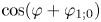 $\cos (\varphi + \varphi _{1;0})$, thus confirming that the higher-order modes are suppressed compared to the first-order one. Panels (aiii,biii) depict the configurations just before the stripes break. Finally, column (iv) shows the equilibrium configurations, which are a drop for the smaller stripe and a band, wrapping around the torus along the
 $\theta$ coordinate, for the larger one. Animations of the time development of the instability for the 2 cases shown in figure 15 are available as supplementary movies 1 and 2.
Time evolution of two unstable stripes on the torus with  $a = 0.4$. (a) The stripe is initialised at
 $\theta _c^{eq}=0.86{\rm \pi}$ and leads after breaking into a droplet configuration equilibrated on the outer side of the torus (animation available as supplementary movie 1). (b) The stripe is initialised at
 $\theta _c^{eq}=0.65{\rm \pi}$ and merges in the poloidal direction after breaking to form a band configuration (animation available as supplementary movie 2). In (a,b), (i) shows the initial conditions, with perturbations along the
 $\varphi$ direction on both interfaces; (ii) and (iii) contain intermediate snapshots of the configurations; and (iv) shows the final equilibrium configurations.

The fact that the stripe configurations lead to droplets or bands indicates that these latter configurations correspond to lower values of the free energy. Under the assumption that the free energy is related to the interface length, we note that, according to (6.3), the interface length for the stripe configuration can vary as the stripe area grows between  $\ell _{\mathit {stripe}}^{min} = 4{\rm \pi} (R - r)$ for infinitesimally small stripes (the two interfaces are at
 $\theta = {\rm \pi}$) and
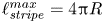 $\ell _{\mathit {stripe}}^{max} = 4{\rm \pi} R$ for the largest stripe, covering half of the torus and having the interfaces at
 $\theta = 0$ and
 ${\rm \pi}$. (We note that, as revealed in § SM:2.3, the free energy for the stripe configurations is just
 $\Psi = \sigma \ell _{\mathit {total}} + O(\xi ^2)$. This simple relation may not hold for more general domain shapes.)
For sufficiently small domain areas, the interface length of a droplet configuration grows with the domain area roughly as 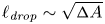 $\ell _{\mathit {drop}} \sim \sqrt {{\rm \Delta} A}$, vanishing as
 ${\rm \Delta} A \rightarrow 0$. Thus, at sufficiently small domain areas, the droplet is energetically preferred.
The band configuration has a domain area-independent interface length, given by the two boundary circles located at constant  $\varphi$,
 $\ell _{\mathit {band}} = 4{\rm \pi} r$. For sufficiently large domain areas,
 $\ell _{\mathit {band}}$ will be smaller than
 $\ell _{\mathit {stripe}}$, since
 $\ell _{\mathit {stripe}}^{\textit{max}} = 4{\rm \pi} R > 4{\rm \pi} r$. In fact, the band configuration can be energetically preferable to the stripe configurations for any domain size when
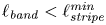 $\ell _{\mathit {band}} < \ell _{\mathit {stripe}}^{\textit{min}}$, which is always satisfied when
 $a < \frac {1}{2}$.
A more comprehensive analysis of the energy landscape, indicating which configurations correspond to the minimum of the free energy, would require a detailed study of the droplet and band configurations, which is beyond the scope of this work. However, based on the discussion in the previous paragraph, it is safe to conclude that there are domains of the subcritical and supercritical regions shown in figure 14(a) where the stripe configurations are actually only metastable.
6.3. Laplace pressure
We now seek for an expression for the pressure difference  ${\rm \Delta} P$ between the two fluid components. For a small increase
 $\delta {\rm \Delta} A$ of the stripe area, let
 $\delta \ell _{\mathit {total}}$ be the increase in the interface length. These two quantities can be related through the equation
 \begin{equation} {\rm \Delta} P \delta {\rm \Delta} A = \sigma \delta \ell_{\mathit{total}}. \end{equation}
The variations  $\delta {\rm \Delta} A$ and
 $\delta \ell _{\mathit {total}}$ can be computed using (6.2) and (6.3)
 \begin{align} \delta {\rm \Delta} A = 4 {\rm \pi}r R \left(1 + a \cos\theta_c \cos \frac{{\rm \Delta} \theta}{2}\right) \delta \frac{{\rm \Delta} \theta}{2}, \quad \delta \ell_{\mathit{total}} = -4{\rm \pi} r \cos \theta_c \sin\frac{{\rm \Delta} \theta}{2} \delta \frac{{\rm \Delta} \theta}{2}.\notag\\ \end{align}
Thus, the pressure difference  ${\rm \Delta} P$ can be written as
 \begin{equation} {\rm \Delta} P = -\frac{\sigma}{R} \frac{\cos\theta_c \sin({\rm \Delta} \theta / 2)} {1 + a \cos\theta_c \cos({\rm \Delta} \theta / 2)}.\end{equation}
The above expression is valid regardless of where the stripe is positioned.
Assuming that the stripe is already in its equilibrium position, (6.27) reduces to
 \begin{equation} {\rm \Delta} P =
\begin{cases} {\displaystyle \frac{\sigma}{R}
\frac{\sin({\rm \Delta} \theta_{eq} / 2)} {1 - a \cos({\rm \Delta}
\theta_{eq} / 2)}}, & {\rm \Delta} A < {\rm \Delta} A_{\mathit{crit}}
\text{ and } \theta_c^{eq}= {\rm \pi},\\ {\displaystyle
\frac{\sigma}{r} \cot \frac{{\rm \Delta} \theta_{eq}}{2}}, &
{\rm \Delta} A > {\rm \Delta} A_{\mathit{crit}} \text{ and } a \cos
\theta_c^{eq} + \cos\dfrac{{\rm \Delta} \theta_{eq}}{2} = 0.
\end{cases}\end{equation}
Equation (6.28) loses relevance in the domain of stripe instability discussed in § 6.2, unless strict axisymmetry is enforced. On the instability line, where (6.22) and (6.23) hold, we find
 \begin{equation} {\rm \Delta} P_{\mathit{inst}} = \frac{\sigma}{R}, \end{equation}
which, remarkably, is independent of  $a$.
We now propose the benchmark test concerning stripe configurations, consisting of the generalisation of the Laplace–Young pressure test. An alternative derivation of (6.27) in the context of the Cahn–Hilliard model considered in this paper is provided in § SM:2.1 of the supplementary material. It is interesting to note that the Laplace pressure is related to a non-vanishing value of the chemical potential when the stripe is in equilibrium. This in turn induces an offset in the order parameter, denoted using  $\phi _0$ and computed in SM:2.21 of the supplementary material.
We perform a series of numerical simulations in the absence of hydrodynamics at three values of  $a$, namely
 $a=0.25$,
 $0.4$ and
 $0.5$, by fixing the outer radius to
 $R=2$ and setting the inner radius to
 $r=\{0.5,0.8,1.0\}$, while keeping
 $M = 2.5 \times 10^{-3}$,
 $\kappa = 5 \times 10^{-4}$ and
 $A = 0.5$ unchanged. We consider stripes of various areas
 ${\rm \Delta} A$. For each value of
 ${\rm \Delta} A$, the equilibrium position
 $\theta _c^{eq}$ is computed and the stripe is initialised using a hyperbolic tangent profile,
 \begin{equation} \phi = \phi_0 + \tanh \zeta, \quad \zeta = \frac{r}{\xi_0 \sqrt{2}}\left( |\widetilde{\theta - \theta_c}| - \frac{{\rm \Delta} \theta}{2}\right), \end{equation}
and centred on 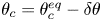 $\theta _c = \theta _c^{eq} - \delta \theta$, with
 $\delta \theta = 0.05 {\rm \pi}$. The notation
 $\widetilde{\theta - \theta_c}$ indicates that the angular difference
 $\theta - \theta_c$ takes values between
 $-{\rm \pi}$ and
 ${\rm \pi}$. The initial width
 ${\rm \Delta} \theta$ is obtained by numerically solving (6.2) for fixed
 ${\rm \Delta} A$ and
 $\theta _c$. The value of
 $\phi _0$ corresponding to the initial stripe centre
 $\theta _c$ and initial width
 ${\rm \Delta} \theta$ is derived in § SM:2.1 of the supplementary material. It is given by
 \begin{equation} \phi_0 = \frac{\xi_0}{3R \sqrt{2}} \frac{\cos\theta_c \sin({\rm \Delta} \theta / 2)} {1 + a \cos\theta_c \cos ({\rm \Delta} \theta/2)}. \end{equation}
After initialisation, the stripes slowly migrate towards the equilibrium positions, as discussed in the § SM:2.4 of the supplementary material. In order to reach the stationary state, we performed  $4 \times 10^9$ iterations at
 $\delta t = 0.002$. After the stationary state was reached, we measured the pressure
 $P_{\textit{binary}} = A(-\frac {1}{2} \phi ^2 + \frac {3}{4} \phi ^4)$ in the interior and exterior of the stripe and computed the difference
 ${\rm \Delta} P$ between these two values. The results are shown using dotted lines and symbols in figure 16. The shaded region indicates the region where the stripes become unstable once the axisymmetric assumption is removed in the model. It is bounded from above by the pressure difference value
 ${\rm \Delta} P_{\mathit {inst}}$ on the instability line, given in (6.29). We observe an excellent agreement with the analytic result, (6.28), which is shown using solid lines.
Comparison of numerical results obtained for  $a = 0.25$ (solid squares),
 $a=0.4$ (solid circles) and
 $a=0.5$ (solid triangles) against the analytic formula (6.28). The system parameters are
 $A = 0.5$,
 $\kappa = 5 \times 10^{-4}$ and
 $M = \tau = 2.5 \times 10^{-3}$. The simulations are performed using
 $N_\theta =\{200,320,400\}$ nodes along the
 $\theta$ direction for
 $r=\{0.5,0.8,1.0\}$, while the time step was set to
 $\delta t = 2 \times 10^{-3}$. The shaded region corresponds to the stripes which are unstable when the axisymmetric assumption is lifted.

It is worth noting that the second-order phase transition observed in the stripe equilibrium positions when  ${\rm \Delta} A = {\rm \Delta} A_{\mathit {crit}}$ is also visible in the dependence of
 ${\rm \Delta} P$ on
 ${\rm \Delta} A$ in figure 16. Its non-monotonic behaviour can be understood as follows. For infinitesimally small stripes, the torus curvature is negligible and no pressure difference can be seen across the interface, as is also the case for the Cartesian (flat space) geometry. As the stripe width
 ${\rm \Delta} \theta$ increases,
 ${\rm \Delta} P$ also increases. In general, a turning point in the Laplace pressure can be expected. This is because the pressure difference vanishes for infinitesimal stripes (
 ${\rm \Delta} \theta \rightarrow 0$), as well as in the opposite case, when the stripe occupies the top or bottom halves of the torus (
 ${\rm \Delta} \theta \rightarrow {\rm \pi}$). In the latter case, the conjugate domain can be obtained from the stripe by employing a symmetry transformation,
 $z \leftrightarrow -z$, which also changes the torus into itself. Thus, the configurations corresponding to the stripe and its conjugate are perfectly equivalent and one can expect there to be no pressure difference across the interface. When the equilibrium position of the stripe is always centred on
 $\theta _c^{eq} = {\rm \pi}$, a smooth dependence of
 ${\rm \Delta} P$ on
 ${\rm \Delta} \theta$ can be expected. However, the phase transition at
 ${\rm \Delta} A = {\rm \Delta} A_{\mathit {crit}}$ which causes the stripe to detach form
 $\theta _c = {\rm \pi}$ leads to the sharp change observed in figure 16.
7. Evolution of fluid stripes in a Cahn–Hilliard multicomponent fluid
In this section we consider the dynamics of the axisymmetric fluid stripes discussed in § 6. Here, we focus on the case where the Cahn–Hilliard equation is fully coupled with hydrodynamics, when the stripes undergo underdamped oscillatory motion towards their equilibrium positions. The relaxation dynamics in the absence of hydrodynamics is discussed in detail in § SM:2.4 of the supplementary material, where we are able to obtain a semi-analytical description of how the stripes relax exponentially to their equilibrium positions. From the perspective of benchmarking Navier–Stokes solver on non-uniform curved surfaces, this section is a culmination of the various ingredients developed in §§ 3, 5 and 6. In particular, we find that the dynamics is governed to leading order by the zeroth-order mode of the velocity derived in (3.23), which corresponds to incompressible flow. This section is structured as follows. The general solution for the underdamped oscillatory motion is presented in § 7.1. A benchmark test is proposed in § 7.2.
7.1. General solution
To derive the stripe dynamics, our starting point is the Cauchy equation in the linearised regime
 \begin{align} \frac{\partial u^{\hat{\theta}}}{\partial t} &= -\frac{k_B T}{m r} \frac{\partial \delta \rho}{\partial \theta} + \frac{\nu}{r^2 (1 + a\cos\theta)^2} \frac{\partial}{\partial\theta} \left[(1 + a \cos\theta)^3 \frac{\partial}{\partial \theta} \left(\frac{u^{\hat{\theta}}}{1 + a\cos\theta}\right)\right] \nonumber\\ &\quad +\frac{\nu_{v}}{r^2} \frac{\partial}{\partial \theta} \left\{\frac{\partial_\theta[u^{\hat{\theta}}(1 + a \cos\theta)]} {1 + a \cos\theta}\right\} - \frac{\phi}{\rho_0 r} \frac{\partial \mu}{\partial \theta}. \end{align}
As in § 3 and 5, we will employ the decomposition written in (3.18) for  $u^{\hat {\theta }}$. Moreover, we will also take advantage of the fact that the higher-order terms
 $U_{c,n}$ and
 $U_{s,n}$ (
 $n > 0$) are damped at a significantly higher rate than the fundamental term
 $U_0$. Then, in order to track the evolution of
 $U_0$, we multiply (7.1) with
 $f_0 / 2{\rm \pi} = (1-a^2)^{1/4} / 2{\rm \pi}$, and integrate it over
 $\theta$ between
 $0$ and
 $2{\rm \pi}$, to obtain
 \begin{equation} \dot{U}_0 + \frac{2\nu a^2}{r^2(1 -a^2)} U_0 + \frac{(1-a^2)^{1/4}}{2{\rm \pi} \rho_0 r} I_\mu \simeq 0, \quad I_\mu = \int_0^{2{\rm \pi}} \textrm{d}\theta \phi \frac{\partial \mu}{\partial \theta}, \end{equation}
where the  $\simeq$ sign indicates that the nonlinear terms, as well as the components of
 $u^{\hat {\theta }}$ with
 $n > 0$, have been neglected. Employing integration by parts,
 $I_\mu$ can be written as
 \begin{equation} I_\mu = \int_0^{2{\rm \pi}} \textrm{d}\theta \left[A \frac{\partial}{\partial \theta} \left(\frac{\phi^2}{2} - \frac{\phi^4}{4}\right) + \frac{\kappa}{r^2}\frac{\partial \phi}{\partial \theta} \frac{\partial^2 \phi}{\partial \theta^2} - \frac{\kappa}{r^2} \frac{a \sin\theta}{1 + a\cos\theta} \left(\frac{\partial \phi}{\partial \theta}\right)^2 \right]. \end{equation}
The first and second terms above do not contribute to the integral. To evaluate the integral of the third term, we assume that  $\phi$ is approximately given by the hyperbolic tangent profile in (6.30) and employ the procedure introduced in § SM:2.1 of the supplementary material, which we briefly review here. First, the integration variable is changed to
 $\vartheta = \theta - \theta _c$ and the integration domain is shifted to
 $-{\rm \pi} < \vartheta < {\rm \pi}$. Then, the flip
 $\vartheta \rightarrow -\vartheta$ is performed on the negative (
 $\vartheta < 0$) branch, yielding
 \begin{equation} I_\mu = -{\rm \pi} a A \int_0^{\rm \pi} \frac{\textrm{d}\vartheta}{2{\rm \pi}}\left[ \frac{\sin (\theta_c + \vartheta)}{1 + a \cos(\theta_c + \vartheta)} + \frac{\sin (\theta_c - \vartheta)}{1 + a \cos(\theta_c - \vartheta)}\right] \frac{1}{\cosh^4 \zeta}. \end{equation}
Next, the integration variable is changed to  $\zeta = r \varsigma / \xi _0 \sqrt {2}$, where
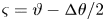 $\varsigma = \vartheta - {\rm \Delta} \theta / 2$, such that the integration domain is
 $- r {\rm \Delta} \theta / \xi _0 \sqrt {8} < \zeta < r(2{\rm \pi} - {\rm \Delta} \theta ) / \xi _0 \sqrt {8}$. Noting that
 $\xi _0 \ll r {\rm \Delta} \theta$, the integration domain can be extended to
 $(-\infty , \infty )$ and
 $I_\mu$ becomes
 \begin{equation} I_\mu = -\frac{3\sigma}{4R} \int_{-\infty}^\infty \dfrac{\textrm{d}\zeta}{\cosh^4 \zeta} \left[ \dfrac{\sin\left(\theta_+ + \dfrac{\xi_0 \zeta\sqrt{2}}{r}\right)} {1 + a \cos \left(\theta_+ + \dfrac{\xi_0 \zeta\sqrt{2}}{r}\right)} + \dfrac{\sin\left(\theta_- - \dfrac{\xi_0 \zeta\sqrt{2}}{r}\right)} {1 + a \cos \left(\theta_- - \dfrac{\xi_0 \zeta\sqrt{2}}{r}\right)}\right], \end{equation}
where 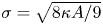 $\sigma = \sqrt {8 \kappa A / 9}$ is the line tension and
 $\theta _\pm = \theta _c \pm {\rm \Delta} \theta / 2$. We now consider an expansion of the integrand with respect to
 $\xi _0 \zeta / r$. The dominant contribution comes from the zeroth-order term. Since the integration domain is even with respect to
 $\zeta$, the first-order term of the expansion does not contribute. Considering that
 $\xi _0 / r \ll 1$, the higher-order terms can be discarded and
 $I_\mu$ can be approximated through
 \begin{equation} I_\mu \simeq -\frac{2\sigma}{R} \frac{\sin\theta_c [a \cos\theta_c + \cos({\rm \Delta} \theta/2)]} {(1 + a \cos\theta_-)(1 + a \cos\theta_+)}. \end{equation}
Substituting (7.6) into (7.2), we obtain
 \begin{equation} \dot{U}_0 + 2\alpha_{\nu} U_0 - \frac{\sigma (1-a^2)^{1/4}}{{\rm \pi} r R \rho_0} \frac{\sin\theta_c [\cos({\rm \Delta} \theta / 2) + a \cos\theta_c]} {(1 + a \cos\theta_-) (1 + a \cos\theta_+)} = 0, \end{equation}
where the viscous damping coefficient  $\alpha _\nu = \nu / (R^2 - r^2)$ is introduced in (5.30).
The relation between  $U_0(t)$ and
 $\theta _c(t)$ can be established by evaluating the Cahn–Hilliard equation on the top and bottom interfaces
 $\theta = \theta _\pm$
 \begin{equation} \frac{r}{\xi_0\sqrt{2}} \left[-\dot{\theta}_+ + \frac{u^{\hat{\theta}}_+}{r} \right] = M ({\rm \Delta} \mu)_+, \quad \frac{r}{\xi_0\sqrt{2}} \left[\dot{\theta}_- - \frac{u^{\hat{\theta}}_-}{r} \right] = M ({\rm \Delta} \mu)_- , \end{equation}
where we have kept the leading-order term of the time derivative of  $\phi$, assuming it takes the hyperbolic tangent profile in (6.30) and evaluating it on the two interfaces
 \begin{equation} \left.\frac{\partial \phi}{\partial t}\right\rfloor_{\theta_\pm}\simeq \mp \frac{r \dot{\theta}_\pm}{\xi_0 \sqrt{2}}. \end{equation}
Subtracting the two equations in (7.8), we obtain
 \begin{equation} \frac{u_+^{\hat{\theta}} + u_-^{\hat{\theta}}}{2r} = \dot{\theta}_c + \frac{\xi_0 M}{r \sqrt{2}} \left[({\rm \Delta} \mu)_+ - ({\rm \Delta} \mu)_-\right]. \end{equation}
On the left-hand side, the velocity profile can be approximated through its zeroth-order term, corresponding to the velocity profile of an incompressible flow
 \begin{equation} u_+^{\hat{\theta}} \simeq \frac{U_0(t) f_0(\theta)}{1 + a \cos\theta_+}, \quad u_-^{\hat{\theta}} \simeq \frac{U_0(t) f_0(\theta)}{1 + a\cos\theta_-}, \end{equation}
as discussed in (3.23). The function  $f_0(\theta ) = (1-a^2)^{1/4}$ is introduced in (3.14). Thus, the left-hand side of (7.10) can be written as
 \begin{equation} \frac{u_+^{\hat{\theta}} + u_-^{\hat{\theta}}}{2r} \simeq \frac{U_0(t) (1 -a^2)^{1/4} [1 + a \cos\theta_c \cos ({\rm \Delta} \theta / 2)]} {r(1 + a \cos\theta_+)(1 + a \cos\theta_-)}. \end{equation}
The right-hand side of (7.10) is identical to the equation for the stripe relaxation dynamics in the absence of hydrodynamics, as discussed in § SM:2.4 of the supplementary material. When hydrodynamics is present, which is the case in this section, the term on the left-hand side dominates over the second term on the right-hand side of (7.10). We will also now consider the linearised limit when 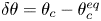 $\delta \theta = \theta _c - \theta _c^{eq}$ is a small quantity. In this case, (7.10) yields
 \begin{equation} U_0(t) = \frac{r(1 + a \cos\theta_+^{eq})(1 + a \cos\theta_-^{eq})} {(1 -a^2)^{1/4} [1 + a \cos\theta_c^{eq} \cos ({\rm \Delta} \theta_{eq} / 2)]} \dot{\delta \theta}. \end{equation}
Taking the derivative of (7.13) allows  $\dot {U}_0$ to be expressed in the linearised limit as
 \begin{equation} \dot{U}_0(t) = \frac{r(1 + a \cos\theta_+^{eq})(1 + a \cos\theta_-^{eq})} {(1 -a^2)^{1/4} [1 + a \cos\theta_c^{eq} \cos ({\rm \Delta} \theta_{eq} / 2)]} \ddot{\delta \theta}. \end{equation}
Equations (7.13) and (7.14) can be inserted into (7.7) to obtain an equation governing the evolution of  $\delta \theta$. The last term in (7.7) can be linearised using (7.15) and (7.16), as follows:
 \begin{equation} \sin \theta_c \left(a \cos\theta_c + \cos\frac{{\rm \Delta} \theta}{2}\right) \simeq -\delta \theta \times \begin{cases} \cos({\rm \Delta} \theta_{eq}/2) - a, & {\rm \Delta} A < {\rm \Delta} A_{\mathit{crit}},\\ 2a \sin^2\theta_c^{eq}, & {\rm \Delta} A > {\rm \Delta} A_{\mathit{crit}}. \end{cases}, \end{equation}
 \begin{equation}(1 + a \cos\theta_+)(1 + a \cos\theta_-) \simeq \begin{cases} [1 - a \cos({\rm \Delta} \theta_{eq}/2)]^2, & {\rm \Delta} A < {\rm \Delta} A_{\mathit{crit}},\\ (1 - a^2) \sin^2 ({\rm \Delta} \theta_{eq} / 2), & {\rm \Delta} A > {\rm \Delta} A_{\mathit{crit}}. \end{cases} \end{equation}
After some rearrangements, the following equation is obtained for  $\delta \theta$:
 \begin{equation} \ddot{\delta \theta} + 2 \alpha_\nu \dot{\delta \theta} + \omega_0^2 \delta \theta = 0. \end{equation}
When  ${\rm \Delta} A < {\rm \Delta} A_{\mathit {crit}}$,
 $\theta _c^{eq} = {\rm \pi}$ and
 $\omega _0^2$ is given by
 \begin{equation} \omega_0^2 = \frac{\sigma \sqrt{1 - a^2}}{{\rm \pi} r^2 R \rho_0} \frac{\cos({\rm \Delta} \theta_{eq} / 2) - a}{[1 - a \cos({\rm \Delta} \theta_{eq} / 2)]^3}. \end{equation}
For  ${\rm \Delta} A > {\rm \Delta} A_{\mathit {crit}}$, the equilibrium position is at
 $\cos ({\rm \Delta} \theta _{eq}/2) + a \cos \theta _c^{eq} = 0$ and
 $\omega _0^2$ is given by
 \begin{equation} \omega_0^2 = \frac{2\sigma}{{\rm \pi} r^3 \rho_0 (1 - a^2)^{3/2}} \frac{a^2 - \cos^2 ({\rm \Delta} \theta_{eq} / 2)}{\sin^2({\rm \Delta} \theta_{eq} / 2)}. \end{equation}
On the instability line, characterised by (6.22) and (6.23), we find
 \begin{equation} \omega_0^2 = \frac{2\sigma a}{{\rm \pi} R^3 \rho_0 (1 - a^2)^{3/2}}. \end{equation}
The general solution of (7.17) is
 \begin{equation} \delta \theta = \delta \theta_0 \cos(\omega_0 t + \vartheta) \,\textrm{e}^{-\alpha_\nu t}, \end{equation}
where  $\delta \theta _0$ and
 $\vartheta$ are integration constants. It is understood that, in the unstable region given by
 $\theta _c < {\rm \pi}- \arctan \,a$ or
 $\theta _c > {\rm \pi}+ \arctan \,a$, the above solution is valid only for strictly axisymmetric flows. In principle, there is a correction to the exponential decay term due to the second term on the right-hand side of (7.10). However, we find that this correction is approximately one or two orders of magnitude smaller than
 $\alpha _\nu$, (a more detailed analysis of the dynamics of stripes in the absence of hydrodynamics can be found in § SM:2.4 of the supplementary material).
7.2. Benchmark test
The solution derived in (7.21) can serve as a benchmark for solvers involving interface dynamics. This benchmark test is particularly difficult since the dynamics of the interface can be significantly altered by numerical artefacts, such as the spurious velocity at the interface, which are known to plague numerical solutions (Sofonea et al. Reference Sofonea, Lamura, Gonnella and Cristea2004; Shan Reference Shan2006).
In the numerical tests discussed below, the velocity field is initialised with  $u^{\hat {\varphi }} = 0$ and
 $\, u^{\hat {\theta }} = U_0 f_0(\theta ) / (1 + a \cos \theta )$, where
 $f_0(\theta ) = (1 - a^2)^{1/4}$ is the zeroth-order harmonic derived in (3.14) and
 $U_0$ is computed based on (7.13) using the solution in (7.21) with
 $\vartheta = 0$ and
 $\dot {\delta \theta } = -\alpha _\nu \delta \theta _0$. The order parameter is initialised with the hyperbolic tangent profile in (6.30).
In the first test, we consider a stripe equilibrating at  $\theta _c^{eq} = {\rm \pi}$, on the torus with
 $R = 2$ and
 $r = 0.8$ (
 $a = 0.4$). The stability region for this torus is
 $0.8789{\rm \pi} < \theta _c^{eq} < 1.1211 {\rm \pi}$. We choose an initial amplitude of
 $\delta \theta _0 = -0.05 {\rm \pi}$ (the initial position is
 $\theta _0 = 0.95 {\rm \pi}$). The initial stripe width is set to
 ${\rm \Delta} \theta _0 = 0.280406 {\rm \pi}$ (at equilibrium,
 ${\rm \Delta} \theta _{eq} \simeq 0.282296 {\rm \pi}\simeq 0.38 {\rm \Delta} \theta _{\mathit {crit}}$). The simulation parameters are
 $\kappa = 2.5 \times 10^{-4}$,
 $A = 0.5$,
 $\nu = M = 2.5 \times 10^{-3}$,
 $\nu _v = 0$ and
 $\rho _0 = 20$, resulting in
 $\omega _0 \simeq 0.0152$ and
 $\alpha _\nu = 7.44 \times 10^{-4}$. The number of nodes and time step are
 $N_\theta = 480$ and
 $\delta t = 5\times 10^{-4}$. The numerical results, shown with red dashed lines and empty circles, are shown alongside the analytical curve corresponding to (7.21) with
 $\vartheta = 0$ and angular velocity
 $\omega _0$ computed using (7.18) in figure 17(a). Without resorting to any fitting routines, it can be seen that the analytic expression provides an excellent match to the simulation results.
Time evolution of the stripe centre  $\theta _c$ for stripes initialised at (a)
 $\theta _0 = 0.95{\rm \pi}$ with
 ${\rm \Delta} \theta _0 = 0.280{\rm \pi}$ (equilibrating at
 $\theta _c^{eq} = {\rm \pi}$, on the torus with
 $a = 0.4$); and (b)
 $\theta_0 = 0.79{\rm \pi}$ with
 ${\rm \Delta}\theta_0= 0.552{\rm \pi}$ (equilibrating at
 $\theta_c^{eq} = 4{\rm \pi}/5$, on the torus with
 $a = 0.8$). The numerical results are shown using dotted lines and symbols, while the analytic solution (7.21) is shown with solid lines.

For the second test, we choose a stripe equilibrating away from  ${\rm \pi}$. In order for this test to be meaningful also when axisymmetry is not strictly imposed, we seek to ensure that the stripe evolution occurs exclusively in the region of stability. For this reason, we increase
 $a$ to
 $0.8$ (
 $R = 2$ remains the same as before and
 $r$ is increased to
 $1.6$), such that the stability region is now
 $0.7853 {\rm \pi}\le \theta _c^{eq} \le 1.2147 {\rm \pi}$. Taking
 $\theta _c^{eq} = 0.8{\rm \pi}$ (corresponding to the equilibrium width
 ${\rm \Delta} \theta _{eq} \simeq 0.551868{\rm \pi} \simeq 1.98 {\rm \Delta} \theta _{\mathit {crit}}$), we choose an initial amplitude of
 $\delta \theta _0 = -0.01{\rm \pi}$, such that
 $\theta _0 = 0.79{\rm \pi}$ and
 ${\rm \Delta} \theta _0 = 0.539376{\rm \pi}$. At larger initial amplitudes, the evolution of the stripe becomes visibly asymmetric, due to the inequivalence between the left and right sides of the equilibrium position. The fluid parameters are set to
 $\kappa = 1.25 \times 10^{-4}$,
 $A = 0.25$,
 $\nu = M = 6.25 \times 10^{-4}$,
 $\nu _v = 0$ and
 $\rho _0 = 20$, resulting in
 $\omega _0 \simeq 8.49 \times 10^{-3}$ and
 $\alpha _\nu \simeq 4.34 \times 10^{-4}$. The number of nodes and time step are set to
 $N_\theta = 960$ and
 $\delta t = 5\times 10^{-3}$. The simulation results, shown using a red dashed line with empty circles, are shown alongside the analytic result, given by (7.21) with
 $\omega _0$ computed using (7.19), are in good agreement, as can be seen from figure 17(b).
We now discuss some of the properties of the oscillation frequency,  $\omega _0$. As can be seen from (7.18) and (7.19),
 $\omega _0^2$ is proportional to the line tension,
 $\sigma$, and inversely proportional to the fluid density,
 $\rho _0$. No explicit dependence can be seen on the viscosities
 $\nu$ and
 $\nu _v$. This is to be expected, since the line tension is responsible for the driving force, while the local mass density is a measure of the fluid inertia.
Keeping  $\rho _0$ and
 $\sigma$ fixed and considering fixed values of the torus radii,
 $r$ and
 $R$,
 $\omega _0$ exhibits a non-monotonic dependence on the stripe width at equilibrium,
 ${\rm \Delta} \theta _{eq}$. Considering that the stripes of negligible width are always subcritical, we have
 $\lim _{{\rm \Delta} \theta _{eq} \rightarrow 0} \omega _0 = \sigma \sqrt {1-a^2} / {\rm \pi}r^2 R \rho _0 (1 - a)^2$. At the other end of the spectrum, stripes with
 ${\rm \Delta} \theta _{eq} = {\rm \pi}$ have
 $\lim _{{\rm \Delta} \theta _{eq} \rightarrow {\rm \pi}} \omega _0 = 2\sigma / {\rm \pi}r R^2 \rho _0 (1 - a^2)^{3/2}$. In between, it can be seen that
 $\omega _0$ vanishes for critical stripes on both the subcritical [(7.18)] and supercritical [(7.19)] branches. This is highlighted in figure 18(a), where
 $\omega _0$ is represented as a function of
 ${\rm \Delta} \theta _{eq}$ for three values of
 $a = r / R$, namely
 $0.3827$ (purple squares),
 $0.7071$ (green circles) and
 $0.9239$ (blue rhombi). These values are chosen such that the critical stripe width is
 ${\rm \Delta} \theta _{eq} = 3{\rm \pi} / 4$,
 ${\rm \pi} /2$ and
 ${\rm \pi} / 4$, respectively. The shaded region marks the instability region, being bounded from below by (7.20). The numerical values of
 $\omega _0$ are obtained by performing a two-parameter fit of (7.21) with respect to
 $\alpha _\nu$ and
 $\omega _0$ (the offset is set to
 $\varsigma = 0$) on the numerical data. The other fluid parameters are
 $\rho _0 = 20$,
 $\nu = 2.5\times 10^{-3}$,
 $\nu _v = 0$,
 $\kappa = 5 \times 10^{-4}$ and
 $A = 0.5$, while
 $R = 2$ is kept fixed. The corresponding analytic results are shown with solid black lines. An excellent agreement can be seen, even for the nearly critical stripe, for which
 $\omega _0$ is greatly decreased.
(a) Comparison between the values of  $\omega _0$ obtained by fitting (7.21) to the numerical results, shown with points, and the analytic expressions, (7.18) for
 ${\rm \Delta} \theta < {\rm \Delta} \theta _{\mathit {crit}}$ (on the descending branch) and (7.19) for
 ${\rm \Delta} \theta > {\rm \Delta} \theta _{\mathit {crit}}$ (on the ascending branch). The radii ratios were chosen such that
 ${\rm \Delta} \theta _{\mathit {crit}}=\{0.25{\rm \pi} ,0.5{\rm \pi} ,0.75{\rm \pi} \}$. The shaded area indicates the region where the stripe configurations are unstable. (b) Colour plot representation of the regularised angular velocity,
 $\overline {\omega }_0$, defined in (7.22), with respect to
 ${\rm \Delta} \theta _{eq} / {\rm \pi}$ (horizontal axis) and
 $a = r / R$ (vertical axis). The green dashed line separates the stability (bottom left) from the instability (top right) regions of the parameter space.

In order to further explore the properties of  $\omega _0$, we focus on its dependence on the stripe width at equilibrium,
 ${\rm \Delta} \theta _{eq}$, and on the torus aspect ratio
 $a = r / R$. From (7.18), it is clear that
 $\omega _0$ diverges as
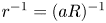 $r^{-1} = (a R)^{-1}$ when
 $a \rightarrow 0$. This is to be expected, since
 $\omega _0$ is proportional to the number of oscillations per unit time, which increases as
 $r$ is decreased. Furthermore, (7.19) shows that when
 $a \rightarrow 1$,
 $\omega _0$ diverges as
 $(1 - a^2)^{-3/4}$. From the above discussion, it is instructive to introduce the dimensionless, regularised oscillation frequency,
 $\overline {\omega }_0$, through
 \begin{equation} \overline{\omega}_0^2
\equiv \frac{{\rm \pi} \rho_0}{4\sigma} r^2 R (1 - a^2)^{3/2}
\omega_0^2 = \begin{cases} {\displaystyle
\frac{[\cos({\rm \Delta} \theta_{eq}/2) - a] (1 - a^2)^2} {4[1 -
a \cos({\rm \Delta} \theta_{eq}/2)]^3}}, & {\rm \Delta} \theta_{eq} <
{\rm \Delta} \theta_{\mathit{crit}},\\
{\displaystyle
\frac{[a^2 - \cos^2({\rm \Delta} \theta_{eq}/2)]} {2a
\sin^2({\rm \Delta} \theta_{eq}/2)}}, & {\rm \Delta} \theta_{eq} >
{\rm \Delta} \theta_{\mathit{crit}}, \end{cases}
\end{equation}
where the factor  ${\rm \pi} / 4$ was introduced for normalisation purposes. It can be seen that
 $\overline {\omega }_0$ attains the maximum value with respect to
 ${\rm \Delta} \theta _{eq}$ when
 ${\rm \Delta} \theta _{eq} \rightarrow 0$. This value is
 \begin{equation} \lim_{{\rm \Delta} \theta_{eq} \rightarrow 0} \overline{\omega}_0 = \frac{1+a}{2}. \end{equation}
The regularised angular velocity  $\overline {\omega }_0$ is represented in figure 18(b) as a function of the stripe width
 ${\rm \Delta} \theta _{eq}/{\rm \pi}$ (on the horizontal axis) and the radii ratio
 $a = r/R$ (on the vertical axis). Due to the chosen normalisation, the colour map spans
 $[0,1]$. The dark line joining the bottom right and top left corners corresponds to the parameters of the critical stripe. The green dashed line delimits the regions of stability (bottom left) and instability (top right).
8. Conclusions
In this work, we focussed on a series of axisymmetric flows on the torus geometry which are solvable analytically. The analytical results are also directly and systematically compared against numerical results obtained using a finite-difference Navier–Stokes solver.
Starting with perfect fluids, we first investigated the propagation of sound waves, identifying the discrete set of frequencies allowed on the torus geometry. In contrast to the planar geometry, the even and odd modes are no longer degenerate. Moreover, since the ratios of the eigenfrequencies are not integers, the periodicity in the fluid flows is lost. We also showed that the sound speed can be altered when changing the equation of state by considering isothermal and thermal ideal fluids, as well as multicomponent flows described via the Cahn–Hilliard equation.
We next looked at the equivalent of the popular shear wave damping problem in Cartesian coordinates. Here, we considered a fluid flowing along the azimuthal direction, with vanishing poloidal velocity. Under the assumption of axial symmetry, we showed that the velocity can be expanded with respect to a discrete set of basis functions which are the eigenfunctions of a second-order differential operator with respect to the poloidal coordinate  $\theta$. The eigenvalues corresponding to these eigenfunctions control the damping rate of the associated velocity components. In particular, we highlighted the relaxation of an initially constant velocity profile towards the zeroth order eigenfunction, corresponding to a vanishing eigenvalue, which corresponds to a non-dissipative flow.
The third problem concerns the damping of sound waves. Here, we discussed the effect of the various dissipative terms appearing in the Navier–Stokes, energy and Cahn–Hilliard equations. Generally, the fluid flow can be decomposed into acoustic modes, which propagate, and thermal/Cahn–Hilliard modes, which simply decay exponentially. The extension of the methodology to other types of fluids is straightforward.
The fourth and fifth phenomena we have studied concern multicomponent flows governed by the Cahn–Hilliard equation. The typical multicomponent axisymmetric configuration that we considered is the stripe, centred on poloidal coordinate  $\theta _c$ and having angular span
 ${\rm \Delta} \theta$.
We showed that, for a general class of multiphase and multicomponent models, the requirement of minimisation of interface length while preserving the stripe area determines the equilibrium position of the stripe. For stripes having a total area less than a critical area  ${\rm \Delta} A_{\mathit {crit}}$, the equilibrium position is on the inside of the torus (
 $\theta _c^{eq} = {\rm \pi}$). As the stripe area is increased above
 ${\rm \Delta} A_{\mathit {crit}}$, two equilibrium positions become possible, highlighting a second-order phase transition in this class of systems. We also generalise the Laplace pressure law. Our analysis gives an exact expression for the difference between the pressure inside of the (minority phase) stripe and the pressure outside of the stripe (i.e. in the majority phase), for both subcritical (
 ${\rm \Delta} A < {\rm \Delta} A_{\mathit {crit}}$) and supercritical (
 ${\rm \Delta} A > {\rm \Delta} A_{\mathit {crit}}$) stripes.
We have also shown that the stripe configurations are not always stable, or even metastable, when axisymmetry is not strictly enforced. For example, the droplet configuration is energetically favoured at small domain areas, while the band configurations, which wrap around the torus along the  $\theta$ direction, are favoured at large domain areas. Moreover, we highlighted that the stripe configurations become unstable to small perturbations when either one of their interfaces crosses the boundary from the region of negative Gaussian curvature (
 ${{\rm \pi} }/{2} < \theta < {3{\rm \pi} }/{2}$) towards the region of positive Gaussian curvature (
 $-{{\rm \pi} }/{2} < \theta < {{\rm \pi} }/{2}$).
Finally, we considered the dynamics of stripes in the presence of hydrodynamics, when the approach to equilibrium of the stripes is achieved through underdamped harmonic oscillations. Using analytical techniques, we find expressions for both the angular velocity and damping coefficient. This is in contrast to the case in the absence of hydrodynamics (detailed in § SM:2.4 of the supplementary material), where the approach to equilibrium is an exponential relaxation.
We believe that the results presented here provide non-trivial problems for developing computational methods for flows on curved surfaces (including the torus), and for benchmarking their accuracy and performance. For instance, the first three flow phenomena in this paper can be used for convergence testing of numerical codes implementing hydrodynamics on curved surfaces. To this end, we present a recipe for performing such tests in appendix A, where we perform a convergence analysis for the numerical scheme employed in this paper. The multicomponent flow phenomena also provide a good example for cases where the Navier–Stokes equation is coupled to other equations capturing more complex physics. For instance, this approach can be adapted to study complex flows on lipid membranes, or to investigate passive and active liquid crystal flows on curved surfaces. Here, the analytical results are limited to the torus geometry and primarily for axisymmetric flows. In the future, it would be interesting to apply and extend the methodology employed here to non-symmetric flow configurations, as well as to other manifolds.
Acknowledgements
H.K. acknowledges funding from EPSRC (EP/J017566/1 and EP/P007139/1). H.K. and V.E.A. also thank the EU COST action MP1305 Flowing Matter (V.E.A. and H.K.; Short Term Scientific Mission 38607). V.E.A. expresses gratitude towards Professor L.-S. Luo (Old Dominion University, Norfolk, VA, USA) for useful discussions and hospitality during the partial completion of this work, as well as towards the Romanian-U.S. Fulbright Commission for generous support through The Fulbright Senior Postdoctoral Program for Visiting Scholars, Grant number 678/2018. S.B. acknowledges funding from EPSRC, grant number EP/R007438/1. V.E.A. and S.B. thank Professor V. Sofonea (Romanian Academy, Timişoara Branch) for encouragement, as well as for sharing with us the computational infrastructure available at the Timişoara Branch of the Romanian Academy. This research was supported by the Research Computing clusters at Old Dominion University. The authors thank Professor A. J. Wagner (North Dakota State University, Fargo, ND, USA) for useful discussions. We thank an anonymous referee for suggesting the stability analysis for the stripe configurations.
Declaration of interests
The authors report no conflict of interest.
Supplementary material and movies
Supplementary material and movies are available at https://doi.org/10.1017/jfm.2020.440.
Appendix A. Convergence test
This section of the appendix illustrates a procedure for using the benchmark problems introduced in §§ 3, 4 and 5 for convergence tests of numerical codes designed for hydrodynamics on curved surfaces. The validation is done against the analytic solutions derived in the aforementioned sections, which are constructed using expansions of the mode functions  $\{\, f_\ell , g_\ell \}$ (for longitudinal waves) and
 $\{F_\ell , G_\ell \}$ (for the shear waves) including terms up to order
 $n$ (
 $3 \le n \le 8$) with respect to the torus radii ratio,
 $a = r / R$. For definiteness, we restrict our convergence study to the amplitudes of the first even harmonic,
 $U_{c;1}(t)$ and
 $V_{c;1}(t)$.
In the first part of this section, we present the validation of our numerical scheme with respect to the spatial resolution. We consider the three benchmark tests described in §§ 3.2, 4.2 and 5.2. Unless otherwise stated, the fluid parameters and initial state are identical to those described in these sections. The numerical values of the amplitudes  $U_{c;1}(t)$ and
 $V_{c;1}(t)$ are obtained as follows. The total simulation time,
 $t_{\textit{max}}$, is divided into
 $S$ intervals
 ${\rm \Delta} t = t_{\textit{max}} / S$, numbered using
 $0 \le s \le S$. At each time
 $t_s = s {\rm \Delta} t$, the numerical solution for the profile of
 $u^{\hat {\theta }}$ or
 $u^{\hat {\varphi }}$ (for the longitudinal or shear wave benchmarks) are projected onto the basis functions
 $f_1(\theta )$ and
 $F_1(\theta )$ using rectangle integration
 \begin{equation} \left.\begin{array}{c@{}} \displaystyle U^{\mathit{num}}_{c;1}(t_s) = \dfrac{1}{N_\theta} \sum_{i = 1}^{N_\theta} \dfrac{u^{\hat{\theta}}_{\mathit{num}}(t_s, \theta_i) f_1(\theta_i)}{1 + a \cos\theta_i}, \\ \displaystyle V^{\mathit{num}}_{c;1}(t_s) = \dfrac{1}{N_\theta} \sum_{i = 1}^{N_\theta} \dfrac{u^{\hat{\varphi}}_{\mathit{num}}(t_s, \theta_i) F_1(\theta_i)}{(1 + a\cos\theta_i)^{-2}}, \end{array}\right\} \end{equation}
where ‘ $\textrm {num}$’ indicates that the amplitudes are determined numerically. The mode functions
 $f_1(\theta )$ and
 $F_1(\theta )$ are computed via the eighth-order expansions with respect to
 $a$ given in SM:3.3a and SM3.4a.
In the context of the propagation of longitudinal waves along the poloidal ( $\theta$) direction through a perfect fluid, figure 19(a) shows the relative error of the angular frequency
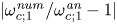 $|\omega _{c;1}^{\mathit {num}}/\omega _{c;1}^{\mathit {an}}-1|$, where
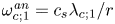 $\omega _{c;1}^{\mathit {an}} = c_s \lambda _{c;1} / r$ is computed using the eighth-order expansion of
 $\lambda _{c;1}$ in SM:3.3b, while the numerical value
 $\omega _{c;1}^{\mathit {num}}$ is obtained using a two-parameter fit of the numerical amplitudes
 $U^{\mathit {num}}_{c;1}(t_s)$ to the analytic prediction in (3.25), i.e.
 \begin{equation} U_{c;1}(t) = {\mathcal{A}} \cos(\omega_{c;1}^{\mathit{num}} t), \end{equation}
where  ${\mathcal {A}}$ and
 $\omega _{c;1}^{\mathit {num}}$ are free parameters. The time interval and total simulation time are taken as
 ${\rm \Delta} t = 0.05$ (corresponding to
 $100$ simulation steps at
 $\delta t = 5\times 10^{-4}$) and
 $t_{\textit{max}} = 18$, such that the total number of intervals is
 $S = 360$. For completeness, we present the results for the isothermal and thermal ideal fluid cases, as well as for the isothermal Cahn–Hilliard multicomponent fluid with background order parameter
 $\phi _0 = 0.8$. The values of the parameters are identical to those considered in § 3.2. It can be seen that all curves are parallel to the slope
 $-5$ dashed line, indicating that our numerical scheme has fifth-order accuracy.
(a) The relative error of  $\omega _{c;1}$ in the context of the inviscid propagation of longitudinal waves, for an isothermal ideal fluid (Iso), an ideal fluid with variable temperature (Th) and an isothermal Cahn–Hilliard multicomponent fluid (CH). (b) The relative error of the damping coefficient
 $\nu \chi _{c;1}^2 / r^2$ in the context of shear wave damping. (c) The relative error of
 $\alpha _{c;1;a}$ in the context of the viscous damping of longitudinal waves, for the same 3 fluid described in (a). Each panel contains a dashed line indicating fifth-order convergence.

We now consider the benchmark problem presented in § 4.2 concerning the damping of shear waves. Figure 19(b) shows the decrease in the relative error of the damping coefficient  $\nu (\chi ^{\mathit {num}}_{c;1})^2 / r^2$ for the amplitude of the first mode,
 $V_{c;1}(t)$, as a function of the number of grid points. The numerical values for the damping coefficient are obtained by fitting the numerical data using the analytic formula obtained by combining (4.13) and (4.10), i.e.
 \begin{equation} V_{c;1}(t) = {\mathcal{A}} \,\textrm{e}^{-\alpha t}, \end{equation}
where  ${\mathcal {A}}$ and
 $\alpha$ are free parameters. The time interval and total simulation time are taken as
 ${\rm \Delta} t = 5$ (corresponding to
 $1000$ simulation steps at
 $\delta t = 5 \times 10^{-3}$) and
 $t_{\textit{max}} = 1800$, such that the total number of intervals is
 $S = 360$. The analytic prediction for
 $\alpha$ is
 $\nu \chi _{c;1}^2 / r^2$. In the log–log plot of figure 19(b), the relative error of the damping coefficient follows the slope
 $-5$ dashed line, also indicating the scheme is fifth-order accurate. The simulation parameters are identical to those considered in § 4.2.
Finally, we consider the sound waves damping benchmark problem introduced in § 5.2. Figure 19(c) presents the relative error for the acoustic damping coefficient  $|1 - \alpha _{c;1;a}^{\mathit {num}}/\alpha _{c;1;a}^{\mathit {an}}|$, where
 $\alpha _{c;1;a}^{\mathit {an}}$ is listed in § 5.2 for the various fluid types considered. Considering the three types of fluids discussed in the first paragraph, these relative errors are plotted with respect to
 $N_\theta$. The values
 $\alpha ^{\mathit {num}}_{c;1;a}$ are obtained by fitting the numerical data using the analytic formula, given in (5.34)
 \begin{equation} U_{c;1}(t) = {\mathcal{A}} \,\textrm{e}^{-\alpha^{\mathit{num}}_{c;1;a} t} \sin (\omega_{c;1}^{\mathit{num}} t), \end{equation}
where  ${\mathcal {A}}$,
 $\alpha ^{\mathit {num}}_{c;1;a}$ and
 $\omega _{c;1}^{\mathit {num}}$ are free parameters. The parameters used in this benchmark test are identical to those in § 5.2 and for definiteness, we focus only on the case when the volumetric kinematic viscosity
 $\nu _v = 0.02$ (the other transport coefficients change from one type of fluid to the other, as described in § 5.2). The time interval and total simulation time are taken as
 ${\rm \Delta} t = 0.05$ (corresponding to
 $100$ simulation steps at
 $\delta t = 5 \times 10^{-4}$) and
 $t_{\textit{max}} = 48$, such that the total number of intervals is
 $S = 960$. It can be seen that the relative error
 $|1 - \alpha ^{\mathit {num}}_{c;1;a} / \alpha ^{\mathit {an}}_{c;1;a}|$ in the acoustic damping coefficient generally follows the slope
 $-5$ dashed line.
In the second part of this section, we consider the effect of varying the expansion order  $n$ of the eigenfunctions, eigenfrequencies and all derived quantities. This study is performed at the level of the
 $L_2$ norms of the errors
 $[U_{c;1}^{\mathit {an}}(t) - U_{c;1}^{\mathit {num}}(t)]/U_0$ and
 $1 - V_{c;1}^{\mathit {num}}(t)/V_{c;1}^{\mathit {an}}(t)$ between the numerical values and analytic predictions for the amplitudes of the first even mode. These norms are computed by integrating over the simulation time using the trapezoidal rule
 \begin{equation} \left.\begin{array}{c@{}} \displaystyle L_2^{\mathit{long}} = \left\{ \dfrac{1}{S} \sum_{s = 0}^S \mathfrak{f}_s \left[\dfrac{U_{c;1}^{\mathit{num}}(t_s) - U_{c;1}^{\mathit{an}}(t_s)}{U_0}\right]^2 \right\}^{1/2},\\ \displaystyle L_2^{\mathit{shear}} = \left\{ \dfrac{1}{S} \sum_{s = 0}^S \mathfrak{f}_s \left[\dfrac{V_{c;1}^{\mathit{num}}(t_s)}{V_{c;1}^{\mathit{an}}(t_s)} - 1\right]^2 \right\}^{1/2}, \end{array}\right\} \end{equation}
where  $\mathfrak{f}_s = 1/2$ when
 $s = 0$ or
 $s = S$ and
 $1$ otherwise. The reason why
 $L_2^{\mathit {long}}$ is computed using absolute [
 $U_{c;1}^{\mathit {num}}(t_s) - U_{c;1}^{\mathit {an}}(t_s)$] rather than relative [
 $U_{c;1}^{\mathit {num}}(t_s)/ U_{c;1}^{\mathit {an}}(t_s) - 1$] differences is that due to the oscillatory nature of
 $U_{c;1}^{\mathit {an}}(t_s)$, there are in principle values of
 $t_s$ where
 $U_{c;1}^{\mathit {an}}(t_s)$ is arbitrarily close to
 $0$. For such values of
 $t_s$, the relative error could be disproportionally large, producing meaningless results. Instead, the relative difference is preferred for
 $V_{c;1}(t_s)$ since
 $V_{c;1}^{\mathit {an}}(t_s)$ exhibits an exponential decay with respect to
 $t_s$. Thus, the absolute differences
 $V_{c;1}^{\mathit {num}}(t_s) - V_{c;1}^{\mathit {an}}(t_s)$ would contribute with an exponentially decreasing amplitude at large times and the result of an
 $L_2$ norm based on the absolute differences would therefore be biased towards the early time properties of
 $V_{c;1}(t)$. The analytical predictions
 $U^{\mathit {an}}_{c;1}(t)$ and
 $V^{\mathit {an}}_{c;1}$ can be obtained from (3.25) and (4.10). The numerical amplitudes
 $U^{\mathit {num}}_{c;1}(t_s)$ and
 $V^{\mathit {num}}_{c;1}(t_s)$ are obtained by projecting
 $u^{\hat {\theta }}_{\mathit {num}}(t_s, \theta )$ and
 $u_{num}^{\hat {\varphi}}(t_s, \theta)$ onto the basis functions
 $f_1(\theta )$ and
 $F_1(\theta )$, as described in (A 1). Both the basis functions and the analytic solutions are obtained using the expansions in SM:3.3a and SM3.4a, truncated at power
 $n$ of the radii ratio
 $a$.
We begin with the benchmark problem introduced in § 3.2, concerning the propagation of longitudinal waves through a perfect fluid. Figure 20(a) shows the variation of  $L_2^{\mathit {long}}$ with respect to the truncation order of the expansion, which is varied between
 $3 \le n \le 8$, for the isothermal and thermal ideal fluid cases, as well as for the isothermal Cahn–Hilliard multicomponent fluid. The simulation parameters are identical to those presented in § 3.2, as well as earlier in this section. In general, an exponential decay of
 $L_2^{\mathit {long}}$ with respect to
 $n$ can be observed for all fluid types considered. A sharper decrease in the
 $L_2$ error norm can be observed when
 $n$ is increased from an odd value to an even one.
The  $L_2$ norm computed using (A 5) in the context of (a) propagation of inviscid longitudinal waves; (b) damping of shear wave; and (c) damping of longitudinal waves. In (a,c), we consider the cases of the isothermal ideal fluid (Iso), ideal fluid with variable temperature (Th) and isothermal Cahn–Hilliard multicomponent fluid (CH). In (b), only the isothermal fluid is considered.

In the context of the shear wave damping benchmark introduced in § 4.2, the analytical expression  $V_{c;1}^{\mathit {an}}(t)$ is obtained by combining (4.13) and (4.10). As before,
 $V_{c;1}^{\mathit {num}}(t)$ is obtained by projecting the velocity profile onto the basis functions
 $F_1$, given in SM3.4a, truncated at order
 $n$. The same order
 $n$ is used to evaluated the analytic prediction
 $V_{c;1}^{\mathit {an}}(t)$. The results are presented in figure 20(b), up to order
 $n=8$. The
 $L_2^{\mathit {shear}}$ decays exponentially and again sharper drops are seen when the expansion order is increased from an odd to an even value. The simulation parameters are identical to those employed in § 4.2. A total of
 $S=360$ time intervals of length
 ${\rm \Delta} t = 1000\delta t = 5$ were saved (
 $t_{\textit{max}} = 1800$).
Lastly, we investigate the convergence of the first harmonic in the context of viscous damping of longitudinal waves. The  $L_2^{\mathit {visc}}$ norm is computed using (A 5), where the analytical prediction for
 $U_{c;1}^{\mathit {an}}(t)$ is given in (5.34). This prediction is evaluated using the values for
 $\omega _1^{\mathit {an}}$ and the integral
 $I_{c;0;1}$ truncated at
 $n$th order. The velocity profile is projected using (A 1) onto the basis function
 $f_1$, computed using a truncation of SM:3.3a at the same order
 $n$, obtaining
 $U_{c;1}^{\mathit {num}}$. The results for the isothermal and thermal ideal fluid cases, as well as for the isothermal Cahn–Hilliard multicomponent fluid are summarised in figure 20(c). Since the linearised theory introduces errors of order
 $O(U_0,\varepsilon ^2)$, in order to reveal the error induced by the expansion order, we decrease the kinematic viscosities employed in § 5.2 for each type of fluid by two orders of magnitude, namely
 $\nu _{\mathit {Iso}}=10^{-4}$,
 $\nu_{Th}=4\times 10^{-5}$ and
 $\nu _{CH}=M\approx 6.486\times 10^{-5}$, while the volumetric kinematic viscosity is set to
 $\nu _v=2\times 10^{-4}$ for all fluid types. The rest of the simulation parameters are:
 $N_\theta =320$,
 $R=2$ and
 $r=0.8$ (
 $a=0.4$),
 $U_0=10^{-5}$ and
 $\delta t=5\times 10^{-4}$. A total of
 $S=500$ time intervals of length
 ${\rm \Delta} t = 1$ were saved (
 $t_{\textit{max}} = 500$). The exponential decay of the
 $L_2^{\mathit {visc}}$ can be clearly seen, and again, a larger decrease can be seen when
 $n$ is increased from an odd to an even value.
Appendix B. Eigenfunctions on the torus
This section of the appendix presents a perturbative procedure for constructing solutions of (3.10) and (4.4) in powers of  $a = r / R$, where
 $r$ and
 $R$ are the inner and outer radii of the torus. Multiplying (3.10) and (4.4) by
 $1 + a\cos \theta$ yields:
 \begin{equation} (1 + a\cos\theta)\left(\frac{\partial^2 \Psi_n}{\partial \theta^2} + \lambda_n^2 \Psi_n\right) + \alpha a\sin\theta \frac{\partial \Psi_n}{\partial \theta} = 0,\end{equation}
where  $\alpha = 1$ and
 $-3$ for (3.10) and (4.4), respectively. We seek solutions of the form
 \begin{equation} \left.\begin{array}{c@{}} \Psi_n = N_n (1 + a \cos\theta)^\alpha \psi_n, \quad \psi_n = \psi_n^{(0)} + a \psi_n^{(1)} + a^2 \psi_n^{(2)} + \dots, \\ \lambda^2_{n} = \lambda^2_{n;0} + a \lambda^2_{n;1} + a^2 \lambda^2_{n;2} + \cdots, \end{array}\right\} \end{equation}
where the normalisation constant  $N_n$ ensures that
 $\Psi _n$ retains unit norm. The prefactor
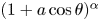 $(1 + a \cos \theta )^\alpha$ ensures that all solutions
 $\Psi _n$ with
 $n > 0$ are exactly orthogonal to the zeroth-order solution as long as they do not contain any free terms. Taking into account this prefactor, (B 1) becomes
 \begin{equation} (1 + a \cos\theta)^2(\psi_n'' + \lambda_n^2 \psi_n) - \alpha a \sin\theta(1 + a \cos\theta) \psi_n' - \alpha a (a + \cos\theta) \psi_n = 0. \end{equation}
Demanding that the coefficient of each power of  $a$ vanishes, at zeroth order the harmonic equation is recovered
 \begin{equation} \psi_{n;0}'' + \lambda_{n;0}^2 \psi_{n;0} = 0.\end{equation}
Furthermore, demanding that the solution at each level of the perturbative analysis be periodic with respect to  $\theta$, the general solution of (B 4) can be written as
 \begin{equation} \psi_{n;0} = \textrm{e}^{\textrm{i} n \theta}, \quad \lambda^2_{n;0} = n^2. \end{equation}
where the real and imaginary parts correspond to the even and odd solutions, respectively.
Taking into account (B 4), the first-order contribution to (B 1) is
 \begin{equation} \psi_{n;1}'' + n^2 \psi_{n;1} + \lambda_{n;1}^2 \,\textrm{e}^{\textrm{i} n \theta} - \frac{\alpha}{2} \left[(n+1) \,\textrm{e}^{\textrm{i}(n+1)\theta} - (n-1)\,\textrm{e}^{\textrm{i}(n - 1)\theta}\right] = 0. \end{equation}
Since the solution of the homogeneous version of the above equation is proportional to  $\psi _{n;0}$, it can be seen that
 $\lambda _{n;1}^2 = 0$, while
 $\psi _{n;1}$ can be found as
 \begin{equation} \psi_{n;1} = -\frac{\alpha}{2} \left[ \frac{n+1}{2n+1} \,\textrm{e}^{\textrm{i}(n+1)\theta} + \frac{n-1}{2n-1} \,\textrm{e}^{\textrm{i}(n-1)\theta}\right]. \end{equation}
At second order, the following equation is obtained:
 \begin{align} &\psi_{n;2}'' + n^2 \psi_{n;2} + \left[\lambda_{n;2}^2 - \frac{\alpha^2 n^2}{2(4n^2 - 1)}\right] \textrm{e}^{\textrm{i}n \theta} + \frac{\alpha (n+2)}{4} \left[1 + \frac{\alpha(n + 1)}{2n+1}\right] \textrm{e}^{\textrm{i}(n+2)\theta} \nonumber\\ &\quad -\frac{\alpha (n-2)}{4} \left[1 + \frac{\alpha(n - 1)}{2n-1}\right] \textrm{e}^{\textrm{i}(n-2)\theta} = 0. \end{align}
As before, the coefficient of  $\textrm {e}^{\textrm {i}n\theta }$ must vanish. At this point, we note that in the case when
 $n = 1$,
 $\textrm {e}^{\textrm {i}(n - 2)\theta } = \textrm {e}^{-\textrm {i}\theta }$ and is thus not independent of
 $\psi _{1;0} = \textrm {e}^{\textrm {i} \theta }$. Moreover, there is no value for
 $\lambda _{1;2}^2$ which ensures that the coefficients of
 $\cos \theta$ and
 $\sin \theta$ vanish simultaneously. Thus, at
 $n = 1$, the solution is
 \begin{equation} \psi_{1;2} = \frac{\alpha(3+2\alpha)}{32}\, \textrm{e}^{3\textrm{i} \theta}, \quad \lambda_{1;c/s;2}^2 = \frac{\alpha^2}{6} \mp \frac{\alpha}{4}, \end{equation}
where the upper and lower signs refer to the even and odd solutions, respectively. For  $n > 1$, the solution is
 \begin{equation} \left.\begin{array}{c@{}} \displaystyle \psi_{n;2} = \dfrac{\alpha}{16} \left[(n-2)\left( \dfrac{1}{n-1} + \dfrac{\alpha}{2n-1}\right) \textrm{e}^{\textrm{i}(n-2)\theta}\right.\\ \displaystyle \qquad + \left.(n+2)\left( \dfrac{1}{n+1} + \dfrac{\alpha}{2n+1}\right) \textrm{e}^{\textrm{i}(n+2)\theta}\right], \\ \displaystyle \lambda_{n;2}^2 = \dfrac{\alpha^2 n^2}{2(4n^2 - 1)}. \end{array}\right\} \end{equation}
Keeping into account that at order  $O(a^{n+1})$, the corrections to the eigenvectors of orders up to
 $n$ must be computed as outlined above for
 $n = 1$, the above procedure can be continued to higher orders. Explicit expressions for the mode functions for
 $\alpha = 1$ (
 $\, f_n$ and
 $g_n$) and for
 $\alpha = -3$ (
 $F_n$ and
 $G_n$) are given in §§ SM:3.1.1 and SM:3.1.2 of the supplementary material.