I. INTRODUCTION
In mechanical analysis, metallic materials are commonly modeled by the elastic-Hollomon power-law hardening hypothesis, in the form of
 $$\left\{ \matrix{ \sigma = E{\rm{\varepsilon }}\quad \left( {{\rm{\varepsilon }} \le {{\rm{\varepsilon }}_{\rm{y}}}} \right) \hfill \cr \sigma = k{{\rm{\varepsilon }}^n} = E{\rm{\varepsilon }}_{\rm{y}}^{1 - n}{\varepsilon ^n}\quad \left( {{\rm{\varepsilon }} > {{\rm{\varepsilon }}_{\rm{y}}}} \right) \hfill \cr} \quad.$$
This form contains three material parameters: the elastic modulus E, the yield strain εy, and the hardening exponent n. Traditionally, uniaxial tension tests are often used to determine these three parameters, in which specially shaped specimens such as dog-bone specimens are needed.
Instrumented indentation tests (IIT) have been recognized as versatile experimental techniques that can provide microdestructive and in situ mechanical testing over multiple scales. In these tests, a specially shaped specimen is not required—only a smooth and flat surface is needed, making the technique convenient and valuable for many applications.
In microscale tests, inhomogeneity of the surface (caused by factors such as different orientations of crystal grains) creates discrepancies when tests are performed over different locations on the surface. Thus, the ability to determine elastic–plastic parameters from a single test is necessary.
Sharp-tipped indenters have been used in IIT more often than other types. However, some investigations have shown that the stress–strain curve cannot be determined by a single sharp-tipped indenter test. Reference Cheng and Cheng1 Therefore, various researchers have investigated test methods that use spherical indenters.
Unfortunately, in most cases, the elastic–plastic parameters were studied separately. Only a few methods have been used to determine elastic–plastic parameters from a single load–depth curve. Reference Hasanov2–Reference Ogasawara, Chiba and Chen4
Some of the previous studies aimed to obtain the stress–strain curve from a load–depth curve.
Reference Hasanov2
However, Liu et al. argued that it was impossible to obtain a unique solution without specific type of work-hardening function.
Reference Liu, Ogasawara, Chiba and Chen5
In other studies, many fitting parameters were involved.
Reference Le3
In this case, it was easy to determine the relationship between the mechanical parameters and the measurement parameters tested. However, these methods led to complex formulations and the parameters lacked theoretical background. Ogasawara et al. obtained elastic–plastic parameters from measurements at several depths, a process that mimics the dual/plural sharp indentation method.
Reference Ogasawara, Chiba and Chen4
However, the expressions for this method at different depths were similar, which may lead to instability of the solution. Moreover, the contact stiffness (used in Ogasawara's method) is determined by the differential method (
 $S = {\left. {\left( {{\mathop{\rm d}\nolimits} F/{\mathop{\rm d}\nolimits} h} \right)} \right|_{h = {h_{\rm{m}}}}}$
), so the accuracy needs to be discussed.
Based on the expanding cavity models, Jiang and Zhang et al. developed a method for determining plastic parameters. Reference Jiang, Zhang, Feng, Yang and Liang6 Two response parameters, the total work W t and the Meyer's coefficient m, were used. W t is related to elastic–plastic parameters as
 $${W_{\rm{t}}} =\, {{2{\rm{\pi }}E{\rm{\varepsilon }}_{\rm{y}}^2{c^3}} \over {3n\left( {n + 1} \right)}}\left[ {{{\left( {{c \over a}} \right)}^{3n}} - 1} \right] +\; {{\left( {n - 1} \right){\rm{\pi }}E{\rm{\varepsilon }}_{\rm{y}}^2{a^3}} \over {3\left( {n + 1} \right)}}\left[ {{{\left( {{c \over a}} \right)}^3} - 1} \right] + \;{{{\rm{\pi }}E{\rm{\varepsilon }}_y^2{c^3}} \over 3}\quad.$$
where W t is the total work, E is the elastic modulus, εy is the yield strain, n is the hardening exponent, a is the radius of the hemispherical hydrostatic core, and c is the radius of the hemispherical hydrostatic plastic zone. m is related to plastic parameters following
 $$\eqalign{ & m = ( - 792.59n^2 + 1675.9n - 962.01){\rm{\varepsilon }}_{\rm{y}}^2 \cr & \quad\quad + (68.187n^2 - 112.78n + 57.84){\rm{\varepsilon }}_{\rm{y}} \cr & \quad \quad- 1.4569n^2 + 2.8637n + 1.7178\quad, \cr}$$
where m is the Meyer's coefficient, εy is the yield strain, and n is the hardening exponent.
When E is known, the plastic parameters can be calculated by solving the two equations. To determine the elastic–plastic parameters at the same time, Jiang et al. combined the expressions for W t and m with the Oliver–Pharr method. Reference Jiang, Zhang and Yang7,Reference Oliver and Pharr8
However, the deviations of the yield strength and elastic modulus obtained from certain indentation tests were at ±40% (mostly within ±25%). Reference Jiang, Zhang and Yang7 To improve the accuracy of the extracted elastic–plastic parameters, in this paper we develop an integrated method. A new equation related to the elastic–plastic parameters is combined with Jiang's method. By solving Eqs. (2) and (3) and the new equation, all three elastic–plastic parameters can be obtained.
II. FORWARD ANALYSIS
A. Unloading work
During the process of unloading, little plastic deformation occurs in the material being tested, and this behavior has been confirmed by finite element analysis. Reference Oliver and Pharr9 Based on this behavior, we assume in this paper that only elastic deformation occurs during unloading. According to the assumption of spherical symmetric of the strain distribution in Johnson's expanding cavity model, Reference Johnson10 the stress p acting on the edge of the spherical cavity [Fig. 1(b)] is reduced to zero during unloading. This behavior means that an elastic stress field caused by −p is added to the elastic–plastic stress field at the end of loading. The elastic stress field can be described by Lamé’s solution Reference Hill11
 $$\left\{ \matrix{ {\rm{\sigma }}_r^{\rm{*}} = - p{{{a^3}} \over {{r^3}}} \hfill \cr {\rm{\sigma }}_{\rm{\theta }}^* = {\rm{\sigma }}_\varphi ^* = p{{{a^3}} \over {2{r^3}}} \hfill \cr} \right.\quad,$$
where a is the radius of the hemispherical hydrostatic core, which can be described as
 $a = \sqrt {2Rh - {h^2}}$
, where R is the radius of the spherical indenter and h is the indentation depth.
Expanding cavity model in which the deformation area below the indenter is divided into three parts. The effect of pile-up or sink-in is equivalent to some fraction of hydrostatic core volume displaced by indenter. (a) The process of loading, which is equivalent to (b) the stress
 $p$
acting on the edge of the spherical cavity.

The spherical stress tensor (
 $\sigma _m^*$
) and equivalent stress (
 ${\tilde \sigma ^*}$
) can be described as
 $$\left\{ \matrix{ {\rm{\sigma }}_m^* = {1 \over 3}{{\rm{\sigma }}_{kk}} = {1 \over 3}\left( {{\rm{\sigma }}_r^* + {\rm{\sigma }}_\theta ^* + {\rm{\sigma }}_\varphi ^*} \right) = 0 \hfill \cr {{{{\tilde \sigma }}}^*} = \sqrt {{3 \over 2}{s_{ij}}{s_{ij}}} = {3 \over 2}{{{a^3}} \over {{r^3}}}p \hfill \cr} \right.\quad,$$
where σ kk is the first stress invariant and s ij is deviator stress tensor.
The density of elastic energy (w e) can be described as
 $$\eqalign{ & w_{\rm{e}} = \int_0^{s_{ij} } {{1 \over {2G}}} s_{ij} {\rm{d}}s_{ij} + \int_0^{\sigma _m } {{{3\left( {1 - 2\nu } \right)} \over E}} {\rm{\sigma }}_m {\rm{d}}\sigma _m \cr & \quad =\; \left. {{1 \over {2G}}{1 \over 2}{2 \over 3}\left( {{3 \over 2}s_{ij} s_{ij} } \right)} \right|_0^{s_{ij} } \;+\; \left. {{{3\left( {1 - 2\nu } \right)} \over E}{1 \over 2}{\rm{\sigma }}_m^2 } \right|_0^{{\rm{\sigma }}_m } \cr & \quad =\; {{1 + \nu } \over {3E}}{{\tilde \sigma }}^2 +\; {{3\left( {1 - 2\nu } \right)} \over {2E}}{\rm{\sigma }}_m^2 \quad, \cr}$$
where G is shear modulus,
 $\nu$
is Poisson's ratio, and E is elastic modulus.
Substituting Eq. (5) into Eq. (6), the density of elastic energy can then be described as
 $$w_{\rm{e}} = {{1 + \nu } \over {3E}}\left( {{{\tilde \sigma }}^* } \right)^2 \;+\; {{3\left( {1 - 2\nu } \right)} \over {2E}}\left( {{\rm{\sigma }}_m^* } \right)^2 \;=\; {{3\left( {1 + \nu } \right)} \over {4E}}{{a^6 } \over {r^6 }}p^2 \quad.$$
Integrating w e over the plastic and the elastic zones (Fig. 1) yields the unloading work,
 $$W_{\rm{e}} = \int_a^\infty {2{\rm{\pi }}rw_{\rm{e}} } dr = {{{\rm{\pi }}\left( {1 + \nu } \right)} \over {2E}}a^3 p^2 \quad.$$


Based on the assumption of elastic unloading, the unloading work W u is the elastic energy released during unloading. Thus,
 $${W_{\rm{u}}} = {W_{\rm{e}}} =\; {{{\rm{\pi }}\left( {1 + \nu } \right)} \over {2E}}{a^3}{p^2}\quad.$$
The stress p comes from the end of loading,
 $$p = {\left. { - {{\rm{\sigma }}_r}} \right|_{r = a}} = - {\left. {{{2E} \over {{\rm{\varepsilon }}_{\rm{y}}^{n - 1}}}\int\!\!\! {\left( {{{{{{{\tilde \varepsilon }}}^n}} \over r}} \right)} {\rm{d}}r} \right|_{r = a}}\quad.$$
The relationship between the equivalent strain
 $\tilde \varepsilon$
and r has been clarified by Yang et al.,
Reference Yang, Zhang and Feng12
 $${{\tilde \varepsilon }} +\; {{4\left( {1 - 2\nu } \right)} \over {3{\rm{\varepsilon }}_{\rm{y}}^{n - 1} }}{{\tilde \varepsilon }}^n =\; {{\left( {7 - 8\nu } \right){\rm{\varepsilon }}_{\rm{y}} } \over 3}{{c^3 } \over {r^3 }}\quad.$$
In Eq. (11), c is the edge of the plastic region, which can be determined by Reference Jiang, Zhang, Feng, Yang and Liang6
 $$\left\{ \matrix{ c = \root 3 \of {{V \over {\pi {\rm{\varepsilon }}_{\rm{y}} }}} \,=\; \kappa \root 3 \of {{{h^2 \left( {3R - h} \right)} \over {3{\rm{\varepsilon }}_{\rm{y}} }}} \hfill \cr \kappa = \left( { -\; 0.0077n^2 + 0.0534n - 0.0304} \right)\log ^2 \left( {{\rm{\varepsilon }}_{\rm{y}} } \right) \hfill \cr \quad\quad +\; \left( {0.3717n^2 - 0.1331n - 0.0774} \right)\log \left( {{\rm{\varepsilon }}_{\rm{y}} } \right) \hfill \cr \quad\quad +\; 0.4950n^2 - 0.3016n + 1.0627 \hfill \cr} \right\quad,$$
where R is the radius of the spherical indenter and h is the indentation depth.
Obtaining an explicit equation of p is impossible by substituting Eq. (11) into Eq. (10). We presume that the second part of Eq. (11) on the left-hand side can be ignored. Thus, Eq. (11) can be reduced to
 $${{\tilde \varepsilon }} =\; {{\left( {7 - 8\nu } \right){{\rm{\varepsilon }}_{\rm{y}}}} \over 3}{{{c^3}} \over {{r^3}}}a\quad.$$
To prove this simplification, we plot the relationship between
 $\tilde \varepsilon$
and r described by Eqs. (11) and (13), respectively (Fig. 2). This figure shows little difference between the values of
 $\tilde \varepsilon$
calculated by Eqs. (11) and (13). Moreover, in Eq. (10), the integration of
 $\tilde \varepsilon$
is used, which reduces the difference between Eqs. (11) and (13).
Substituting Eq. (13) into Eq. (10), an explicit equation for the unloading work can be obtained,
 $$W_{\rm{u}}^* =\; {{{\rm{\pi }}\left( {1 + \nu } \right)E{\rm{\varepsilon }}_{\rm{y}}^2 a^3 } \over 2}\left[ {\left( {{{7 - 8\nu } \over 3}} \right)^n {2 \over {3n}}\left( {{{c^{3n} } \over {a^{3n} }} - 1} \right) + 1} \right]^2 \,\,\,.$$
To confirm the accuracy of this function, we performed finite element calculations using ABAQUS for different combinations of plastic parameters, with E = 200 GPa, εy ranging from 0.0015 to 0.006, and n ranging from 0.05 to 0.3. These parameters encompass those of most metallic materials. The spherical indenter tip was assumed to be rigid. Coulomb's friction law was applied with a value of 0.15 and Poisson's ratio was fixed at 0.3. Both of these parameters are minor factors in the indentation analysis. The relationship between
 ${W_{\rm{u}}}/W_{\rm{u}}^*$
and n is shown by Fig. 3, here, W
u is the unloading work determined from finite element analysis and
 $W_{\rm{u}}^*$
is determined from Eq. (14). The result appears to be a quadratic function, which we fit to the following function:
 $${{{W_{\rm{u}}}} \over {W_{\rm{u}}^*}} \;=\; \left( {242.62{{\rm{\varepsilon }}_{\rm{y}}} - 4.6663} \right){n^2} + \left( { - 268.30{{\rm{\varepsilon }}_{\rm{y}}} + 3.1253} \right)n + \left( {57.053{{\rm{\varepsilon }}_{\rm{y}}} + 0.56730} \right)\quad.$$
Relationship between
 ${W_u}/{W_{u0}}$
and n. By fitting the curve, the correction factor of unloading work can be obtained.

The amended function of unloading work is
 $$\left\{ \matrix{ {W_{\rm{u}}} = \lambda {{\pi \left( {1 + \nu } \right)E\varepsilon _{\rm{y}}^2{a^3}} \over 2}{\left[ {{{\left( {{{7 - 8\nu } \over 3}} \right)}^n}{2 \over {3n}}\left( {{{{c^{3n}}} \over {{a^{3n}}}} - 1} \right) + 1} \right]^2} \hfill \cr \lambda = \left( {242.62{\varepsilon _{\rm{y}}} - 4.6663} \right){n^2} + \left( { - 268.30{\varepsilon _{\rm{y}}} + 3.1253} \right)n +\; \left( {57.053{\varepsilon _{\rm{y}}} + 0.56730} \right) \hfill \cr} \right..$$
B. Similarity solution
The Meyer's coefficient m can be determined by Reference Jiang, Zhang, Feng, Yang and Liang6
 $$m = \,{{\log \left( {F_{0.6} /F_{0.7} } \right)} \over {\log \left( {0.6R/0.7R} \right)}} = 14.9\log \left( {{{F_{0.6} } \over {F_{0.7} }}} \right)\quad,$$
where F 0.6 and F 0.7 are the indentation forces corresponding to a = 0.6R and a = 0.7R, respectively.
The relationship between m and the plastic parameters has been given by Jiang et al. Reference Liu, Ogasawara, Chiba and Chen5 as
 $$\eqalignb{ m = ( - 792.59{n^2} + 1675.9n - 962.01){\rm{\varepsilon }}_{\rm{y}}^2 &\cr \quad + \;(68.187{n^2} - 112.78n + 57.84){{\rm{\varepsilon }}_{\rm{y}}} &\cr \quad -\; 1.4569{n^2} + 2.8637n + 1.7178\quad. &\cr}$$
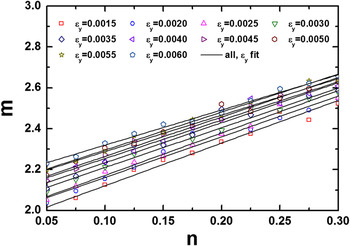
This relationship appears somewhat complicated and increases the instability of the results of reverse analysis. Therefore, we refitted the similarity solution. According to these results of finite element analysis, the Meyer's coefficients for various materials are shown in Fig. 4. A simple linear relationship appears to describe the relationship between m and the plastic parameters. The refitted function of m is given as
 $$m = \left( { - 70.436{\rm{\varepsilon }}_{\rm{y}} + 2.1866} \right)n + \left( {49.355{\rm{\varepsilon }}_{\rm{y}} + 1.8547} \right)\quad.$$
Relationship between the Meyer's coefficient m and the hardening exponent n according to the results of finite element analysis. By fitting the curve, a new expression of the Meyer's coefficient can be obtained.

C. Integrated method
Equation (19) is the function of unloading work and the Meyer's coefficient. Combined with the function of loading work determined by Jiang, the integrated method used for determining elastic–plastic parameters of linear-elastic power-hardening materials has been given as
 $$\left\{ \matrix{ {W_{\rm{t}}} =\, {{2{\rm{\pi }}E{\rm{\varepsilon }}_{\rm{y}}^2{c^3}} \over {3n\left( {n + 1} \right)}}\left[ {{{{c^{3n}}} \over {{a^{3n}}}} - 1} \right] +\, {{\left( {n - 1} \right){\rm{\pi }}E{\rm{\varepsilon }}_{\rm{y}}^2{a^3}} \over {3\left( {n + 1} \right)}}\left[ {{{{c^3}} \over {{a^3}}} - 1} \right] +\, {{{\rm{\pi }}E{\rm{\varepsilon }}_{\rm{y}}^2{c^3}} \over 3} \hfill \cr {W_{\rm{u}}} = \lambda {{{\rm{\pi }}\left( {1 + \nu } \right)E{\rm{\varepsilon }}_{\rm{y}}^2{a^3}} \over 2}{\left[ {{{\left( {{{7 - 8\nu } \over 3}} \right)}^n}{2 \over {3n}}\left( {{{{c^{3n}}} \over {{a^{3n}}}} - 1} \right) + 1} \right]^2} \hfill \cr m = \left( { - 70.436{{\rm{\varepsilon }}_y} + 2.1866} \right)n + \left( {49.355{{\rm{\varepsilon }}_y} + 1.8547} \right) \hfill \cr}\quad.$$
For a given spherical indentation test with a specific range of h/R (0 < h/R < 0.3), W
t and m can be obtained from the loading process of load–depth curve and W
u can be obtained from the unloading process. As an explicit form of analytical expressions, the elastic–plastic parameters (E, εy, and n) can be solved using Newton's iteration method. To obtain a stable solution, we suggest that
 ${W_{\rm{u}}}/{W_{\rm{t}}}$
can be combined with m and E can be eliminated. Thus, εy and n can be solved. Then, substitute εy and n into the expression of either W
t or W
u to solve E.
III. REVERSE ANALYSIS
A. Effectiveness
Numerical indentation simulations are used to examine the effectiveness of the reverse analysis algorithm. Different plastic parameters for the materials were chosen from the following range: εy of (1.5–6.0) × 10−3 and
 $n$
of 0.05–0.3, which encompass most engineering metals. Poisson's ratio was fixed at 0.3. The elastic modulus was fixed at 210 GPa because numerical simulations are dimensionless and the effect of the elastic modulus is linear. To make these simulations consistent with reality, we chose to approximate the elastic modulus of steel by using a value of 210 GPa.
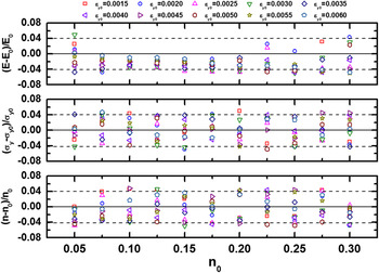
Finite element method (FEM) was carried out using ABAQUS to verify these methods. Combinations of parameters (E, σy, n) were inputted into FEM, and the load–depth curves were used to obtain the indentation parameters (W t, W u, m). The results are shown in Fig. 5, where E 0, σy0, and n 0 represent the input, whereas E, σy, and n are the results predicted by the reverse analysis. By comparing the solution obtained by our new method with the input, it was found that the maximum error is ±5%, which shows that our new method is fairly reliable and has satisfactory accuracy.
Relative deviation of estimated elastic–plastic parameters using the integrated method from the input values. The maximum error is ±5%. This result supports that the integrated method is fairly reliable and has satisfactory accuracy.

B. Sensitivity
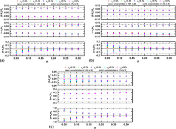
To determine the error of the test results caused by errors in the test parameters, we introduced artificial error into the testing parameters inputted into our method. The elastic–plastic parameters in Sec. III. A were substituted in Eq. (20), and theoretical values of the test parameters were obtained. We then added relative error of ±3% to W t and W u, as well as ±2% to m, and used those parameters with artificial error to determine elastic–plastic parameters. After this, we compared the determined elastic–plastic parameters with the default values. The results of this comparison are shown in Fig. 6. An error of ±3% in W t and W u leads to an error of ∼±7% in E and σy, as well as ±15% in n. An error of ±2% in m leads to an error ∼±5% in E, ±20% in σy, and ±50% in n.
Sensitivity distribution observed when determining the elastic–plastic parameters with uncertainties of (a) +3% and −3% in W t, (b) +3% and −3% in W u, and (c) +2% and −2% in m.

C. Experimental verification
To confirm the reliability of our new method, we selected ten typical materials (Iron DT4, Steel IF, Steel Gr.D, Steel 1045, Al 2024, Al 5083, Al 7075, Copper C11000, Brass C28000, and Ti Grade5), upon which we performed ultrasonic immersion tests, tensile tests, and indention tests. Reference Jiang, Zhang and Yang7 Ultrasonic immersion provided reference elastic parameters, whereas the uniaxial tensile tests provided reference plastic parameters.
1. Ultrasonic immersion tests
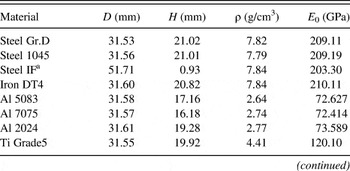
The elastic moduli of the ten materials were determined by ultrasonic immersion tests performed at Research Center for Non-Destructive Testing & Evaluation, Beijing University of Technology. Reference Song, Wei, He and Wu13 Cylindrical specimens with diameters of ∼20 mm and heights of ∼31 mm were used. The diameter D, height H, density ρ, and elastic modulus E 0 for each material are shown in Table I. Here, E 0 is the mean value of the results of our tests, which will be used as a reference.
Dimensions of samples and mean elastic moduli obtained from ultrasonic immersion tests.

a Steel IF and other materials were tested at different times, so the sizes were different. All the tests were performed in the same laboratory.
2. Uniaxial tensile tests
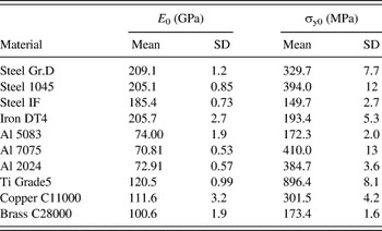
Three dog-bone specimens with square cross sections (5 × 5 mm) made from each of the ten materials considered in this paper were tested by Jiang et al. Reference Jiang, Zhang and Yang7 The elastic modulus E, yield strength σy0, and standard deviations for each material are shown in Table II. σy0 is used as a reference value in the present work.
Elastic moduli and yield strengths obtained from tensile tests. Reference Jiang, Zhang and Yang7

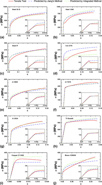
These tensile tests show that some materials cannot be fit well by the ideal power-law expression. It is difficult to obtain an exact result for the hardening exponent by fitting a different range of the σ–ε curve. Therefore, we cannot give a reference value for the hardening exponent. However, the mechanical parameters obtained by the integrated method can be used to predict the σ–ε curve. Thus, we can confirm the accuracy of the hardening exponent by comparing the predicted σ–ε curve with those obtained from the tensile tests.
3. Instrument indentation tests
Spherical indentation tests were performed using a Nano Indenter XP (MTS) by Jiang et al. Reference Jiang, Zhang and Yang7 Averaged load–depth curves from indentation tests are used in this paper.
IV. RESULTS AND DISCUSSION
For a given spherical indentation test, W
t and W
u can be calculated by integrating over the loading and unloading portions of the load–depth curves, respectively. The value of m can be obtained by fitting the gradient of the linear regression of log F and
 $\log a$
for
 $0.2 \lt h/R \lt 0.3$
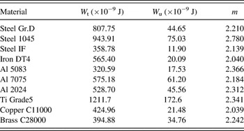
. Extracted values of W
t, W
u, and m for each material are shown in Table III. By substituting W
t, W
u, and
 $m$
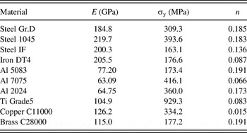
into Eq. (20), we can calculate E, σy, and n, as shown in Table IV.
W t, W u, and m for each material obtained from indentation tests.

Mechanical parameters obtained by indentation tests with the integrated method.

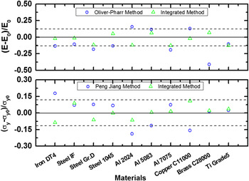
The relative deviations between the indentation tests and the reference values for the ten materials are shown in Fig. 7. In this figure, the reference value of E 0 is obtained from ultrasonic immersion tests, whereas that of σy0 is obtained from uniaxial tensile tests. The elastic modulus E is obtained by the Oliver–Pharr method and the integrated method in this paper. The yield strength σy is obtained by Jiang's method and the integrated method in this paper. The deviations for the values calculated using the integrated method are all within ±13%. This result is better than those calculated using the Oliver–Pharr method and Jiang's method, from which the deviations are about ±25%.
Comparison of elastic modulus and yield strength from indentation tests and the reference values of ten materials.

The obtained parameters (E, σy, and n) can be used to recreate the stress–strain curves by using the power-law hardening relationship in Eq. (1). Figure. 8 shows comparisons of the predicted stress–strain curves by Jiang's method and those by the integrated method in this paper with those obtained from tensile tests. The slope of the linear portion represents the elastic modulus, the intersection of the linear and nonlinear portions represents the yield stress, and the nonlinear portion represents the hardening exponent.
Comparison of true stress–strain curves obtained from indentation and tensile tests for ten metals.

Our integrated method is based on a type of linear-elastic power-law hardening relationship. However, it can be shown that not all of the materials tested (such as Iron DT4) fit the power-law relationship. Thus, attention should be paid when using this method to evaluate unknown materials. More research is needed to determine whether this method can be used to judge the type of work hardening used on a given material.
As suggested by Liu et al., Reference Liu, Ogasawara, Chiba and Chen5 deep spherical indentation is necessary to guarantee a unique solution. However, in this case the scale of indentation may be equal to that of one crystal grain, and the influence of crystal grains has not been discussed.
V. CONCLUSION
In this paper, we established an integrated method to determine the elastic–plastic parameters of materials that harden with a linear-elastic power-law relationship, by combining a function of unloading work (rather than the Oliver–Pharr method) and an existing method for plastic parameters. Only one spherical indenter is needed in our method, and thus the indentation test is greatly simplified. Ten typical metals were selected for experimental verification, and the results of these experiments showed that this method can provide reasonable estimates of the elastic–plastic parameters for most common metals.
ACKNOWLEDGMENTS
We thank Professor Guorong Song from Research Center for Non-Destructive Testing & Evaluation, Beijing University of Technology for her help with the ultrasonic immersion tests.
Authors gratefully acknowledge the financial support from the National Natural Science Foundation of China (Grant Nos. 11025212, 11272318, 11302231, and 11172305).