



1. Introduction
Understanding the flow of particle suspensions is of great importance in many industrial, biological and geophysical applications. Such dispersed particle flows have certain properties that are of interest. For the quality of coatings (Li, Zhu & Zhang Reference Li, Zhu and Zhang2005), the capture rate of plankton (Pésceli, Trulsen & Fiksen Reference Pésceli, Trulsen and Fiksen2012) and the formation of cloud droplets (Balkovsky, Falkovich & Fouxon Reference Balkovsky, Falkovich and Fouxon2001), the spatial distribution of particles within the suspending fluid is of great importance. Particle suspensions usually also have a shear-dependent effective viscosity. In many cases, such as in determining the texture and pumping requirements of food (Bayod & Willers Reference Bayod and Willers2002), understanding the rheology of the suspensions is necessary for design and optimization.
A common way of modelling such properties in suspensions involves assuming that the particles are perfectly spherical, due to the accessibility of models for particle–fluid interactions (Crowe et al. Reference Crowe, Schwarzkopf, Sommerfeld and Tsuji2012). However, assuming the particles to be spherical is insufficient for numerous applications, such as in predicting particle motion of fibres in paper pulp (Lundell, Söderberg & Alfredsson Reference Lundell, Söderberg and Alfredsson2011) and composite moulds (Le et al. Reference Le, Dumont, Orgéas, Favier, Salvo and Boller2008), the motion of asbestos fibres in the respiratory system (Miserocchi et al. Reference Miserocchi, Sancini, Mantegazza and Chiappino2008) or the motion and growth of snow crystals in the atmosphere (Gavze, Pinsky & Khain Reference Gavze, Pinsky and Khain2012). Having a suspension of non-spherical particles presents an additional challenge, as properties become dependent not only on the spatial distribution of particles but also on the orientation distribution; in order to understand the physics of the collective orientation distribution of non-spherical particles, one needs to know how a single particle rotates due to local velocity gradients in the flow, and how this affects the rheology.
In the present work, we consider a single prolate spheroidal particle in a simple shear flow, which is ideally created through the induced flow of two parallel, opposite moving walls (figure 1). The flow will affect the particle through forces on the particle surface and give rise to a torque on the particle. This in turn yields a rotational motion. In the absence of fluid and particle inertia, analytical expressions for this rotational motion were derived by Jeffery (Reference Jeffery1922). The particle was found to move periodically in one of an infinite number of closed kayaking orbits around the vorticity axis (figure 2
c; the kayaking state can be described as a precession and nutation around the vorticity axis). It was later seen in experiments (Taylor Reference Taylor1923; Binder Reference Binder1939; Karnis, Goldsmith & Mason Reference Karnis, Goldsmith and Mason1963) that upon including fluid inertia, the particle has a preferred orbit of tumbling (rotation around the minor axis, which is aligned with the vorticity axis; see figure 2
a) or log-rolling (rotation around the major axis, which is aligned with the vorticity axis; see figure 2
b), depending on the aspect ratio
 $r_{p}$
and the particle Reynolds number
 $\mathit{Re}_{p}$
.
A spheroidal particle is placed in a linear shear flow generated by two parallel, opposite moving walls; the orientation of the particle is described by the angles
 ${\it\phi}$
and
 ${\it\theta}$
; the angle
 ${\it\psi}$
is of less interest for spheroids due to the rotational symmetry of the particle.

Rotational states of the prolate spheroid in a linear shear flow: (a) tumbling (
 $\dot{{\it\phi}}=f({\it\phi})$
) or rotating (
 $\dot{{\it\phi}}=\text{const.}$
); (b) log-rolling; (c) kayaking; (d) inclined rolling; (e) inclined kayaking; (f) steady state (where the particle symmetry axis is located in the flow-gradient plane, making an angle
 ${\it\phi}_{c}$
with the flow (i.e.
 $x$
) direction); (a, f) are planar rotational states (
 ${\it\theta}={\rm\pi}/2$
), while (b–e) are non-planar (
 $0\leqslant {\it\theta}<{\rm\pi}/2$
); the rotational states can also be viewed in a movie clip provided in the supplementary data.

Theoretical studies have shown that the leading effect of fluid inertia is a drift towards log-rolling for nearly spherical particles (Saffman Reference Saffman1956; Subramanian & Koch Reference Subramanian and Koch2006), whereas slender fibers drift towards tumbling (Subramanian & Koch Reference Subramanian and Koch2005). Numerical results have also shown that there exists a critical Reynolds number
 $\mathit{Re}_{p}=\mathit{Re}_{c}$
, above which a motionless (steady) state exists (figure 2
f), such that the particle major axis is perpendicular to the vorticity axis and makes a small angle
 ${\it\phi}_{c}$
to the flow direction (Aidun, Lu & Ding Reference Aidun, Lu and Ding1998; Ding & Aidun Reference Ding and Aidun2000; Zettner & Yoda Reference Zettner and Yoda2001; Subramanian & Koch Reference Subramanian and Koch2005; Huang, Wu & Lu Reference Huang, Wu and Lu2012a
; Huang et al.
Reference Huang, Yang, Krafczyk and Lu2012b
; Rosén, Lundell & Aidun Reference Rosén, Lundell and Aidun2014).
Particle inertia, associated with the Stokes number
 $\mathit{St}$
, leads to a drift towards tumbling (Subramanian & Koch Reference Subramanian and Koch2006; Lundell & Carlsson Reference Lundell and Carlsson2010) if fluid inertia is negligible. Furthermore, very heavy particles have been observed to undergo a transition from tumbling (where angular velocity is dependent on orientation) to rotating (where angular velocity is constant) (Lundell & Carlsson Reference Lundell and Carlsson2010; Nilsen & Andersson Reference Nilsen and Andersson2013). Computer simulations that include fluid and particle dynamics have proven to be a very useful tool for studying the full three-dimensional rotational behaviour of particles. Qi & Luo (Reference Qi and Luo2002, Reference Qi and Luo2003) found that a neutrally buoyant spheroid (with the particle having the same density as the fluid) of aspect ratio (major axis/minor axis)
 $r_{p}=2$
was tumbling at low
 $\mathit{Re}_{p}$
but log-rolling at high
 $\mathit{Re}_{p}$
. However, their study considered only two initial orientations, and from this they claimed that the final rotational state was independent of initial orientation. Recent numerical work has shown that there exist several other equilibrium rotational states when
 $\mathit{Re}_{p}$
is increased, including inclined rolling, inclined kayaking and kayaking (Yu, Phan-Thien & Tanner Reference Yu, Phan-Thien and Tanner2007; Huang et al.
Reference Huang, Yang, Krafczyk and Lu2012b
; Rosén et al.
Reference Rosén, Lundell and Aidun2014). These rotational states are illustrated in figure 2(c–e). It was also observed that these states always coexist with a stable tumbling solution, and that the final state depends on the initial orientation. Even though previous numerical works (Qi & Luo Reference Qi and Luo2002, Reference Qi and Luo2003; Yu et al.
Reference Yu, Phan-Thien and Tanner2007; Huang et al.
Reference Huang, Yang, Krafczyk and Lu2012b
; Rosén et al.
Reference Rosén, Lundell and Aidun2014) agree qualitatively, the quantitative critical values of
 $\mathit{Re}_{p}$
characterizing the transitions differ between the studies. The reasons for these discrepancies are believed to be differences in spatial resolution and the fact that determination of these parameters is very sensitive to how well the boundary layer around the particle is resolved. This issue will be investigated thoroughly in the present work. What is also missing from most numerical studies is discussion of the fact that
 $\mathit{Re}_{p}$
and
 $\mathit{St}$
are dependent on one another through the relation
 $\mathit{St}={\it\alpha}\mathit{Re}_{p}$
, where
 ${\it\alpha}$
is the solid-to-fluid density ratio. This relationship means that even a neutrally buoyant particle will experience particle inertial effects for
 $\mathit{Re}_{p}>0$
, since
 $\mathit{St}=\mathit{Re}_{p}$
in that case.
Each rotational state mentioned here is associated with fluid and/or particle inertial effects being dominant, and can be seen as a combination of two dynamical states for the fluid and the particle. The dominant inertial effects for the different states are summarized in table 1. Generally, particle inertia is the dominant effect if the final rotational state is a time-periodic state for both particle and fluid, whereas fluid inertia dominates if the final rotational state is a steady-state solution for the fluid. All the rotational states discussed in this work are illustrated in a movie clip, available as supplementary data at http://dx.doi.org/10.1017/jfm.2015.127.
Description of the rotational states of the particle, together with their abbreviations, and the corresponding states in terms of fluid and particle dynamics.

Just as in previous work, a distinction will be made between planar rotational states and non-planar rotational states. In planar states, including the tumbling, rotating and steady states, the particle symmetry axis is located in the flow-gradient plane (
 ${\it\theta}={\rm\pi}/2$
); in the non-planar states, i.e. log-rolling, inclined rolling, inclined kayaking and kayaking, the particle symmetry axis is located at
 $0\leqslant {\it\theta}<{\rm\pi}/2$
.
The previous results indicate that the final rotational state is dependent not only on
 $\mathit{Re}_{p}$
but also on
 $\mathit{St}$
, since these parameters control the competition between fluid inertia and particle inertia. This competition determines most of the transitions between the rotational states in table 1, and examining the state space in the
 $\mathit{Re}_{p}$
–
 $\mathit{St}$
plane is necessary to understanding the physical mechanisms. At this point, it is appropriate to comment on the effect of gravity, since
 $\mathit{St}\neq \mathit{Re}_{p}$
means that the solid-to-fluid density ratio is not equal to
 $1$
. Obviously, sedimentation in itself affects particle rotation at non-zero Reynolds numbers. When combined with shear, a huge parameter space opens up (both the direction and the strength of gravity must be considered), but this is beyond the scope of the present study. For the case of small
 $\mathit{Re}_{p}$
and
 $\mathit{St}$
and nearly spherical particles, a perturbation analysis including sedimentation was done by Subramanian & Koch (Reference Subramanian and Koch2006), but for wider ranges of
 $\mathit{Re}_{p}$
,
 $\mathit{St}$
and
 $r_{p}$
complete parameter sweeps are unfeasible. Nevertheless, the identification of critical transitions in the
 $\mathit{Re}_{p}$
–
 $\mathit{St}$
plane will help to reduce the complexity of future studies. Similar arguments can be made when it comes to other aspects that affect rotation, such as Brownian diffusion.
Still, previous studies have almost solely been concerned with neutrally buoyant (
 ${\it\alpha}=1$
) spheroidal particles of fixed aspect ratio. Here, we extend the work of Rosén et al. (Reference Rosén, Lundell and Aidun2014) to cover all the rotational states of a prolate spheroidal particle in a
 $\mathit{Re}_{p}$
–
 $\mathit{St}$
parameter space and also look closely at the transitions as functions of the particle aspect ratio
 $r_{p}$
. The aim of this work is to predict the rotational behaviour of a prolate spheroidal particle with any density and aspect ratio in the absence of gravity. We will also discuss the implications this has for the rheological behaviour of dilute suspensions of such particles.
The outline of the paper is as follows. Section 2 will cover the flow problem and the range of parameters used in this numerical study. Section 3 will explain in detail the important knowledge gained from the works of Lundell & Carlsson (Reference Lundell and Carlsson2010) (only particle inertial effects) and Rosén et al. (Reference Rosén, Lundell and Aidun2014) (only neutrally buoyant particles of
 $r_{p}=4$
) and show that a general description of the flow problem has not yet been obtained. In § 4, we first discuss the difficulties in obtaining quantitative results due to the sensitivity to grid resolution; secondly, the qualitative rotational dynamics in the entire
 $\mathit{Re}_{p}$
–
 $\mathit{St}$
parameter space will be described for a particle of aspect ratio
 $r_{p}=4$
(the same aspect ratio as in Rosén et al. (Reference Rosén, Lundell and Aidun2014)). Finally, in § 5 we discuss how the dynamics changes with the aspect ratio
 $r_{p}$
.
2. Method
The method used in the present work is the lattice Boltzmann method with external boundary forcing (LB-EBF). A description of the computational method can be found in appendix A, and further details are provided in the work by Wu & Aidun (Reference Wu and Aidun2010). For the case of a spheroidal particle in a shear flow, the method was also validated and verified by Rosén et al. (Reference Rosén, Lundell and Aidun2014) and so will not be repeated here. Only the case of
 ${\it\alpha}\geqslant 1$
(i.e. the particle has density equal to or higher than the surrounding fluid) will be simulated in this study, but the explanation of the physical processes will allow us to predict the behaviour of light particles (with
 ${\it\alpha}<1$
) as well.
2.1. The flow problem
The problem is set up by simulating the flow between two parallel moving walls located at
 $y=0$
and
 $y=N$
moving with velocities
 $U$
and
 $-U$
, respectively, in the
 $x$
direction. The boundaries at
 $x=0$
,
 $x=N$
,
 $z=0$
and
 $z=N$
are treated with periodic boundary conditions. The linear shear flow has a shear rate of
 $G=2U/N$
, which is also the relevant inverse time scale for the flow problem. The prolate particle, placed in the middle of the domain, is described by the equation
 $$\begin{eqnarray}\frac{x^{\prime 2}}{a^{2}}+\frac{y^{\prime 2}}{b^{2}}+\frac{z^{\prime 2}}{b^{2}}=1\end{eqnarray}$$
where
 $(x^{\prime },y^{\prime },z^{\prime })$
denotes a body-fixed coordinate system. The length of the prolate particle symmetry axis
 $a$
is greater than the equatorial radius
 $b$
, and we define an aspect ratio
 $r_{p}=a/b$
. The orientation and rotation of the particle are defined according to figure 1 with the Euler angles
 $({\it\phi},{\it\theta},{\it\psi})$
, and a corresponding rotational velocity vector is defined as
 ${\bf\omega}=(\dot{{\it\phi}},\dot{{\it\theta}},\dot{{\it\psi}})$
. The important dimensionless numbers in this problem are the aspect ratio
 $r_{p}$
, the particle Reynolds number
 $\mathit{Re}_{p}$
(associated with fluid inertia) and the Stokes number
 $\mathit{St}$
(associated with particle inertia). The latter two quantities are defined as
 $$\begin{eqnarray}\displaystyle & \displaystyle \mathit{Re}_{p}=\frac{4\,Ga^{2}}{{\it\nu}}, & \displaystyle\end{eqnarray}$$
 $$\begin{eqnarray}\displaystyle & \mathit{St}={\it\alpha}\,\mathit{Re}_{p}, & \displaystyle\end{eqnarray}$$
 ${\it\nu}$
is the kinematic viscosity of the fluid and
 ${\it\alpha}$
is the solid-to-fluid density ratio.
The aim of the present work is to determine the rotational motion of a spheroidal particle solely due to shear, while all forces giving a translational motion (e.g. gravity) are neglected.
The domain is chosen to be cubic with confinement
 ${\it\kappa}=2a/N=0.2$
to ensure results independent of domain size, as demonstrated by Rosén et al. (Reference Rosén, Lundell and Aidun2014). A too-high confinement can influence the dynamics since streamlines close to the walls are forced to be in the horizontal direction. To get good resolution of the surface forces on the particle, the minor semi-axis was limited to
 $b\geqslant 3$
and the major semi-axis restricted to
 $a\geqslant 12$
, where the length unit is the side of the cubic lattice. The lower limits were set by considering the smallest particle that still undergoes the same sequence of transitions as a larger particle. In particular, a neutrally buoyant particle of
 $a=24$
and
 $b=6$
was simulated with
 $N=240$
and
 $G=1/1200$
and was observed to undergo the same transitions with increasing
 $\mathit{Re}_{p}$
(not presented in detail here) as a particle with
 $a=12$
and
 $b=3$
. We also mention here that the correct Reynolds number for describing the flow around the minor axis should be equal to
 $\mathit{Re}_{p}/r_{p}^{2}$
. This means that the flow is much less complex around the minor dimension compared with that around the major dimension, and therefore the fluid–solid interaction is better captured when particle is in a non-planar motion (Do-Quang et al.
Reference Do-Quang, Amberg, Brethouwer and Johansson2014). Consequently, mesh convergence is ensured for the dynamics and any influence of a low mesh number can be ruled out. To simulate a spheroidal particle of aspect ratio
 $r_{p}>4$
(i.e.
 $a>12$
), the domain size was increased to ensure that
 ${\it\kappa}=0.2$
, but with the shape remaining cubic. To simulate such low confinement, the range of
 $\mathit{Re}_{p}$
is constrained since the flow becomes unstable at a too-high channel Reynolds number
 $\mathit{Re}_{H}={\it\kappa}^{-2}\,\mathit{Re}_{p}$
. In the range of
 $\mathit{Re}_{p}=10{-}300$
, the particle could reach its final rotational state before the flow becomes unsteady and non-periodic; hence this is considered a valid range for the problem. The lower limit on
 $\mathit{Re}_{p}$
was set to ensure a low value of the lattice Boltzmann viscosity
 ${\it\nu}$
, which is connected to the Knudsen number through
 $\mathit{Kn}=\sqrt{3}{\it\nu}/(2a)$
, and thus to ensure the absence of slipping effects at constant shear rate
 $G$
(Rosén et al.
Reference Rosén, Lundell and Aidun2014).
In general, throughout this study, all transitional Reynolds numbers are determined with an accuracy of
 ${\rm\Delta}\mathit{Re}_{p}=1$
, meaning that if a transition is found at
 $\mathit{Re}_{p}$
and not at
 $\mathit{Re}_{p}+{\rm\Delta}\mathit{Re}_{p}$
, a transition is said to have occurred at
 $\mathit{Re}_{p}+{\rm\Delta}\mathit{Re}_{p}/2$
. The same determination is used for critical Stokes numbers, with
 ${\rm\Delta}\mathit{St}=10$
.
3. Summary of previous knowledge
3.1. Heavy particle in creeping shear flow
Jeffery (Reference Jeffery1922) derived analytical expressions for the torque on an ellipsoidal particle in a linear Stokes flow (
 $\mathit{Re}_{p}=0$
) for any angular velocity vector. By coupling this torque to the equation of motion for the particle, a differential equation could be obtained and integrated, which was done numerically by Lundell & Carlsson (Reference Lundell and Carlsson2010). This differential equation in non-dimensional form has a dependency on the Stokes number
 $\mathit{St}={\it\alpha}\,\mathit{Re}_{p}$
, which determines the effect of particle inertia relative to viscous forces. Even though the torque was derived for
 $\mathit{Re}_{p}=0$
, a solution could be found for finite
 $\mathit{St}$
. The Stokes flow solution can, however, be considered valid even in a low-
 $\mathit{Re}_{p}$
regime. As mentioned in the introduction, Lundell & Carlsson (Reference Lundell and Carlsson2010) and Nilsen & Andersson (Reference Nilsen and Andersson2013) reported a transition for elongated heavy spheroids in linear shear flow from tumbling to rotating, due to particle inertial forces dominating viscous damping forces. The period is found to be a decreasing function of the Stokes number, with the period
 $GT_{J}=2{\rm\pi}(r_{p}^{-1}+r_{p})$
obtained at
 $\mathit{St}=0$
and the period
 $GT_{H}=4{\rm\pi}$
as
 $\mathit{St}\rightarrow \infty$
. The transition is characterized by
 $\mathit{St}_{0.5}$
, which is defined as the Stokes number at which the spheroid rotates with a period of
 $(GT_{J}+GT_{H})/2$
. For a particle of
 $r_{p}=4$
, this number is
 $\mathit{St}_{0.5}=307$
, and was observed by Lundell & Carlsson (Reference Lundell and Carlsson2010) to be an increasing function of
 $r_{p}$
. It should be mentioned that for a particle with this quite low value of
 $r_{p}$
, the transition from tumbling to rotating will be rather smooth since
 $GT_{J}=8.5{\rm\pi}$
, which is not much larger than
 $GT_{H}=4{\rm\pi}$
. For a more slender particle the transition is sharper, as was also observed by Lundell & Carlsson (Reference Lundell and Carlsson2010) and Nilsen & Andersson (Reference Nilsen and Andersson2013).
The transition is illustrated in figure 3, where the angular velocity in the final rotational state is plotted against the angle at different
 $\mathit{St}$
values. In the figure, a comparison is also made with the present LB-EBF model, where a prolate spheroid with
 $r_{p}=4~(a=12,b=3)$
is simulated for
 $\mathit{Re}_{p}=0.5$
(with shear rate lowered to
 $G=1/34\,560$
to ensure low
 $\mathit{Kn}$
) in a computational domain of
 $N=120$
. The density ratio was chosen to be
 ${\it\alpha}=2\times 10^{0},2\times 10^{1},\dots ,2\times 10^{5}$
, leading to the same range of Stokes numbers as in the analytical case. The simulated results are compared with the analytical results at the same Stokes number. The simulated results agree well with the analytical ones, with some small discrepancies which can be explained by the slight non-zero
 $\mathit{Re}_{p}$
in the simulations.
Phase diagrams showing the motion of a spheroid with
 $r_{p}=4$
in a flow with negligible fluid inertia: our numerical model at
 $\mathit{Re}_{p}=0.5$
(circles) is compared with analytical results from Lundell & Carlsson (Reference Lundell and Carlsson2010) (solid lines) for: (a)
 $\mathit{St}=1$
; (b)
 $\mathit{St}=10$
; (c)
 $\mathit{St}=100$
; (d)
 $\mathit{St}=1000$
; (e)
 $\mathit{St}=10\,000$
; (f)
 $\mathit{St}=100\,000$
. Panels (a)–(f) show the transitions from tumbling to rotating; in each panel the dashed line indicates the location of
 $\dot{{\it\phi}}_{min}$
during a period.

3.2. Neutrally buoyant particle (
 ${\it\alpha}=1,r_{p}=4$
) at
$\mathit{Re}_{p}>0$


Rosén et al. (Reference Rosén, Lundell and Aidun2014) investigated a prolate spheroid with
 $r_{p}=4$
and reported that the particle inertia and fluid inertia are always in competition, even for a neutrally buoyant particle. As fluid inertia, associated with
 $\mathit{Re}_{p}$
, increases, particle inertia also increases since it is associated with the Stokes number
 $\mathit{St}=1\cdot \mathit{Re}_{p}$
. Therefore, if the particle is released at an orientation where the symmetry axis gains enough angular momentum, centrifugal forces will take it to a planar tumbling motion. Otherwise, fluid inertia effects will dominate, leading to non-planar motion (i.e. log-rolling, inclined rolling, inclined kayaking or kayaking). At
 $\mathit{Re}_{p}>\mathit{Re}_{c}$
, fluid inertia can be strong enough to completely stop the motion, and the particle will end up in a steady state. The transitions for a neutrally buoyant particle with
 $r_{p}=4$
, as found by Rosén et al. (Reference Rosén, Lundell and Aidun2014), are summarized in table 2, and the dynamical behaviour at
 $\mathit{Re}_{p}=60$
(T/LR), 70 (T/IR), 74 (T/IK) and 80 (T) is shown in figure 4.
Summary of all dynamical transitions of a neutrally buoyant spheroidal particle with
 $r_{p}=4$
in a linear shear flow, as found by Rosén et al. (Reference Rosén, Lundell and Aidun2014).

Trajectories of a neutrally buoyant particle with
 $r_{p}=4$
initialized at rest from five different initial orientations: (a) particle motion projected onto the
 $xy$
-plane by
 $(p_{x},p_{y})=(\sin {\it\theta}\cos {\it\phi},\sin {\it\theta}\sin {\it\phi})$
; (b) the five initial orientations according to (3.1) projected onto the
 $xy$
-plane, where the grey circles indicate the initial conditions, which due to symmetry in the flow problem are equivalent to the initial orientations 2–5, and the large circle represents orientations in the flow-gradient plane (when the particle is in planar rotation at
 ${\it\theta}={\rm\pi}/2$
); projected trajectories from simulations at (c)
 $\mathit{Re}_{p}=60$
, (d)
 $\mathit{Re}_{p}=70$
, (e)
 $\mathit{Re}_{p}=74$
and (f)
 $\mathit{Re}_{p}=80$
, where the empty circles represent the initial orientations and the filled circles the orientations at
 $G\cdot t=1000$
.

In the subcritical Hopf bifurcation at
 $\mathit{Re}_{\mathit{LR}}$
, the log-rolling solution is stabilized, and there are two coexisting stable rotational states, one of which is associated with fluid inertial effects (log-rolling) and the other with particle inertial effects (tumbling). An unstable limit cycle (sketched as a dashed curve in figure 4
b,c) is created in this transition. This limit cycle is located between the two solutions and distinguishes the initial orientations that lead to each rotational state. To illustrate this, a particle is simulated at
 $\mathit{Re}_{p}=60,70,74$
and 80 with five different initial orientations according to
 $$\begin{eqnarray}\left.\begin{array}{@{}c@{}}({\it\phi}_{0},{\it\theta}_{0})_{1}=(0,0),\\ \displaystyle ({\it\phi}_{0},{\it\theta}_{0})_{2{-}5}=\left(\frac{{\rm\pi}n}{2},\frac{{\rm\pi}m}{8}\right),\quad n=0,1~\text{and}~m=1,2.\end{array}\right\}\end{eqnarray}$$
In figure 4(a) the projection
 $(p_{x},p_{y})=(\sin {\it\theta}\cos {\it\phi},\sin {\it\theta}\sin {\it\phi})$
of a simulated particle trajectory is displayed, and figure 4(b) shows the projection of the five initial orientations from (3.1). Figure 4(c) shows that at
 $\mathit{Re}_{p}=60$
, the initial orientations 1, 2 and 4 are inside the unstable limit cycle and lead to log-rolling, whereas the initial orientations 3 and 5 are outside the limit cycle and end up in the tumbling state. The size of the limit cycle thus determines how probable it is that a random orientational configuration of particles, initialized at rest, will end up in the log-rolling state. After the supercritical pitchfork bifurcation at
 $\mathit{Re}_{\mathit{PF}}$
, the unstable limit cycle shrinks and reshapes, as can be seen in figure 4(d,e); finally, the limit cycle is annihilated in a saddle-node bifurcation of limit cycles at
 $\mathit{Re}_{T}$
, as seen in figure 4(f).
The transition at
 $\mathit{Re}_{p}=\mathit{Re}_{c}$
, for a particle of
 $r_{p}=4$
, is through an infinite-period saddle-node bifurcation with a diverging tumbling period close to
 $\mathit{Re}_{p}=\mathit{Re}_{c}$
(Ding & Aidun Reference Ding and Aidun2000; Rosén et al.
Reference Rosén, Lundell and Aidun2014). The bifurcation gives rise to two equilibrium orientations, where there is zero torque on the particle: one stable orientation
 ${\it\phi}_{c}$
and one unstable orientation
 ${\it\phi}_{us}$
; see figure 5. This means that for a small deviation
 ${\it\phi}_{c}\pm {\it\delta}{\it\phi}$
or
 ${\it\phi}_{us}+{\it\delta}{\it\phi}$
, the particle will go to
 ${\it\phi}_{c}$
, but a small negative deviation
 ${\it\phi}_{us}-{\it\delta}{\it\phi}$
will make the particle rotate around the vorticity direction until it is almost aligned with the flow again at
 ${\it\phi}_{c}-{\rm\pi}$
. The transition at
 $\mathit{Re}_{c}$
is based on the balance between the torque on the particle from the primary flow and the opposing torque from the secondary flow, as explained in Ding & Aidun (Reference Ding and Aidun2000). The magnitude of the torque from the secondary flow increases with the Reynolds number, and at the critical value it balances the torque from the primary flow. The quantitative value of
 $\mathit{Re}_{c}$
predicted numerically depends on the exact point of balance reached. This makes the value of
 $\mathit{Re}_{c}$
strongly dependent on precise prediction of the flow around the particle. This is true also for determination of the exact values of
 $\mathit{Re}_{PF},\mathit{Re}_{\mathit{Hopf}}$
and
 $\mathit{Re}_{T}$
.
Illustration of equilibrium angles at
 $\mathit{Re}_{p}>\mathit{Re}_{c}$
: (a) stable equilibrium angle at
 ${\it\phi}_{c}$
; (b) unstable equilibrium angle at
 ${\it\phi}_{us}$
.

3.3. Bifurcation diagram
In practical applications, the solid-to-fluid density ratio of the particle and fluid rarely varies; instead, it is of greater significance what the rotational states of the particles are with constant
 ${\it\alpha}$
and varying
 $\mathit{Re}_{p}$
. This is best illustrated with a bifurcation diagram, shown in figure 6, following Rosén et al. (Reference Rosén, Lundell and Aidun2014).
To draw bifurcation diagrams, a norm is needed to distinguish between the different rotational states. Rosén et al. (Reference Rosén, Lundell and Aidun2014) used the measure
 $N_{C}=C_{norm}(1+|{\bf\omega}/G|)$
, where
 $C_{norm}$
is an orbit parameter defined as
 $$\begin{eqnarray}\left.\begin{array}{@{}c@{}}\displaystyle C_{norm}=\frac{C}{C+1},\\ C=r_{p}^{-1}\tan {\it\theta}(r_{p}^{2}\sin ^{2}{\it\phi}+\cos ^{2}{\it\phi})^{1/2}.\end{array}\right\}\end{eqnarray}$$
This yields:
-
(i)
$N_{C}=\text{const.}$
-
(a)
$N_{C}=0$
, log-rolling; -
(b)
$0<N_{C}<1$
, inclined rolling; -
(c)
$N_{C}=1$
, steady state;
-
-
(ii)
$N_{C}=f(t)$
-
(a)
$N_{C,mean}\geqslant 0.5$
, tumbling/rotating; -
(b)
$N_{C,mean}<0.5$
, inclined kayaking, kayaking.
-


The definition above also makes it easy to distinguish planar rotational states (
 $N_{C}\geqslant 1$
) from non-planar rotational states (
 $N_{C}<1$
). The oscillating states for which
 $N_{C}=f(t)$
are shown by plotting
 $N_{C,max}$
and
 $N_{C,min}$
during a period, represented by the grey area in figure 6. The dashed lines illustrate the approximate location of unstable fixed points, while the open circles illustrate the approximate location of
 $N_{C,max}$
of the unstable cycles. The bifurcation diagram reveals the following hysteresis behaviour: if one starts on the non-planar branch (where
 $N_{C}<1$
) and increases or decreases
 $\mathit{Re}_{p}$
, the particle will eventually end up in a tumbling motion for
 $\mathit{Re}_{p}>\mathit{Re}_{T}$
or
 $\mathit{Re}_{p}<\mathit{Re}_{\mathit{LR}}$
; however, since the tumbling solution is also available at
 $\mathit{Re}_{\mathit{LR}}<\mathit{Re}_{p}<\mathit{Re}_{T}$
, if
 $\mathit{Re}_{p}$
is now varied the particle will always stay in this planar motion.
Bifurcation diagram for a spheroid with
 $r_{p}=4$
; the zoomed-in region with
 $\mathit{Re}_{p}$
between 60 and 100 is displayed on the right. The stable rotational states have either a fixed orientation (solid lines) or an oscillating orientation (grey area), where in the latter case the norm is plotted using
 $N_{C,max}$
and
 $N_{C,min}$
during an oscillation period; the unstable fixed points are schematically drawn with dashed lines, and the approximate location of
 $N_{C,max}$
for the unstable limit cycle is indicated by the open circles.

3.4. Motivation for the present work
The knowledge from previous work can be summarized in
 $\mathit{Re}_{p}$
–
 $\mathit{St}$
parameter space, as is done in figure 7 for a prolate spheroid with
 $r_{p}=4$
. The entire regime of
 $\mathit{St}>0$
and
 $\mathit{Re}_{p}=0$
is well understood from the work of Lundell & Carlsson (Reference Lundell and Carlsson2010), and the line where
 $\mathit{St}=\mathit{Re}_{p}$
, i.e.
 ${\it\alpha}=1$
, is well understood from the work of Rosén et al. (Reference Rosén, Lundell and Aidun2014) and others.
Dynamical transitions of a prolate spheroidal particle with
 $r_{p}=4$
in the
 $\mathit{Re}_{p}$
–
 $\mathit{St}$
parameter space, as known from previous work by Lundell & Carlsson (Reference Lundell and Carlsson2010) and Rosén et al. (Reference Rosén, Lundell and Aidun2014). As in table 1,
 $\text{T}=\text{tumbling}$
,
 $\text{R}=\text{rotating}$
,
 $\text{LR}=\text{log-rolling}$
,
 $\text{IR}=\text{inclined rolling}$
,
 $\text{IK}=\text{inclined kayaking}$
,
 $\text{K}=\text{kayaking}$
and
 $\text{S}=\text{steady state}$
.

The region where
 $\mathit{St}>\mathit{Re}_{p}$
is not well documented. The critical Reynolds number
 $\mathit{Re}_{c}$
is defined for a stationary particle and hence is dependent only on the geometry of the problem; this number therefore cannot depend on
 $\mathit{St}$
. The dependence of the other critical Reynolds numbers (
 $\mathit{Re}_{\mathit{LR}}$
,
 $\mathit{Re}_{PF}$
,
 $\mathit{Re}_{\mathit{Hopf}}$
and
 $\mathit{Re}_{T}$
) on the Stokes number was not known prior to this work. Furthermore, the dependence of
 $\mathit{St}_{0.5}$
on
 $\mathit{Re}_{p}$
and how all these transitions depend on the aspect ratio
 $r_{p}$
are also not clear. All of these questions will be addressed in this work, where a complete picture of the dynamics of a single prolate spheroid will be provided. The results help to explain contradictions in the literature and provide a complete framework for analysing rotational motion of a particle in shear flow.
4. Results: dynamics of a spheroid with
$r_{p}=4$

4.1. Comments about the sensitivity of
$\mathit{Re}_{c}$
to the flow field near the particle

The transition at
 $\mathit{Re}_{c}$
is very sensitive to small changes in the fluid field around the particle, as it is caused by a very delicate balance of torques on the particle. At
 $\mathit{Re}_{p}=\mathit{Re}_{c}$
, the negative torque
 $T^{-}$
from the primary flow is exactly equal to the positive torque
 $T^{+}$
from the secondary flow (illustrated in figure 8). Therefore, a small error of
 $\pm 1\,\%$
in determining
 $T^{+}$
or
 $T^{-}$
can lead to a large error in the value of
 $\mathit{Re}_{c}$
. This stringent requirement of accuracy in determining the torque results in difficulty pinpointing the critical Reynolds number using any numerical method without extreme grid refinement around the particle.
Qualitative flow field close to steady state at
 $\mathit{Re}_{p}\approx \mathit{Re}_{c}$
; the primary flow (1) gives a negative torque (clockwise direction in left panel) on the particle, and the secondary flow (2) gives a positive torque (anticlockwise direction in left panel) on the particle (Ding & Aidun Reference Ding and Aidun2000).

The aim of the present work is to describe dynamical states of the particle in shear flow, and a moving grid is therefore crucial. The qualitative changes in the fluid field as
 $\mathit{Re}_{p}$
changes are not sensitive to resolution, so the order in which the dynamical states occur and the particle behaviour in each dynamical region are resolution-independent. This is probably why the sensitivity described above has not been reported before. For example, the present model matches the transitional Reynolds numbers of Huang et al. (Reference Huang, Yang, Krafczyk and Lu2012b
) when the same resolution is used (Rosén et al.
Reference Rosén, Lundell and Aidun2014). The critical Reynolds number
 $\mathit{Re}_{c}$
was estimated by Huang et al. (Reference Huang, Yang, Krafczyk and Lu2012b
) to be
 $\mathit{Re}_{c}=445\pm 5$
for the case of
 $r_{p}=2$
and
 ${\it\kappa}=0.5$
.
Special consideration must be given to two parameters in lattice Boltzmann methods, due to the kinetic basis of the approach. One consideration is that the maximum Knudsen number
 $\mathit{Kn}_{max}$
must be small enough in order to correctly describe a continuum fluid. This number is defined close to
 $\mathit{Re}_{c}$
as
 $\mathit{Kn}_{max}=2\sqrt{3}\,a\,Gr_{p}/\mathit{Re}_{c}$
, and can be seen in figure 9(b) to be small (approximately
 $O(10^{-3})$
) and decreasing with
 $N$
. These effects are therefore considered negligible. The second consideration is that the maximum lattice Boltzmann Mach number in the simulation,
 $Ma_{max}$
, should be small in order to eliminate any compressible effects in the fluid. This number is linearly increasing with
 $N$
via the relation
 $Ma_{max}=\sqrt{3}GN/2$
. Therefore, to keep
 $Ma_{max}$
small, as
 $N$
increases
 $G$
must become smaller to keep
 $GN$
small. The smaller the value of
 $G$
, the larger the number of time steps required to reach the equilibrium state. To pinpoint the quantitative value of
 $\mathit{Re}_{c}$
requires very large
 $N$
, very small
 $G$
and very long computational time. However, in order to capture the dynamics of the particle motion and the equilibrium states, it is not necessary to pinpoint the value of
 $\mathit{Re}_{c}$
.
Resolution dependence of the critical Reynolds number
 $\mathit{Re}_{c}$
for a prolate spheroid with
 $r_{p}=4~(a=N/10)$
and
 ${\it\kappa}=0.2$
: (a)
 $\mathit{Re}_{c}$
versus the spatial resolution
 $N$
with constant shear rate
 $G=1/2400$
or
 $G=1/1800$
; (b)
 $Ma_{max}$
and
 $\mathit{Kn}_{max}$
versus the spatial resolution
 $N$
.

To investigate the desired range of
 $\mathit{Re}_{p}$
, the shear rate was set to
 $G=1/600$
, which was seen by Rosén et al. (Reference Rosén, Lundell and Aidun2014) to give correct behaviour of particle motion. However, the physical transitional
 $\mathit{Re}_{p}$
values, for example
 $\mathit{Re}_{c}$
, could differ from the values presented here, since
 $G$
is not small enough (and
 $N$
not large enough) for the solution to have converged to the precise value of
 $\mathit{Re}_{c}$
(Rosén et al.
Reference Rosén, Lundell and Aidun2014). Figure 9 shows that the value of
 $\mathit{Re}_{p}$
converges to the accurate
 $\mathit{Re}_{c}$
as the resolution
 $N$
increases (with particle size determined by
 $a=N/10$
). It is found that, due to the slow convergence with respect to the spatial resolution, getting a converged value of
 $\mathit{Re}_{c}$
will be extremely computationally expensive; the values obtained are in the range of 69–132.
Consequently, to obtain a converged solution of
 $\mathit{Re}_{c}$
not only requires high spatial resolution through a high value of
 $N$
but also a low value of the shear rate
 $G$
in order to be able to neglect compressible effects. Because the lattice Boltzmann equation is explicit in time integration, the shear rate
 $G$
is simultaneously connected to the time resolution of the particle rotation, and more time steps are required for lower values of
 $G$
. Furthermore, as
 $\mathit{Re}_{p}$
approaches the critical point, i.e.
 $\mathit{Re}_{c}$
, the period of oscillation increases to infinity asymptotically. In essence, the computational cost of achieving a simulation that is fully converged in space with a low
 $Ma_{max}$
is huge.
However, a ‘steady state’ approach can be employed to accurately pinpoint
 $\mathit{Re}_{c}$
, as shown by Ding & Aidun (Reference Ding and Aidun2000). Determining the value of
 $\mathit{Re}_{c}$
does not require performing a transient simulation, since it is defined as the minimum
 $\mathit{Re}_{p}$
at which a stationary particle with a certain orientation
 ${\it\phi}~({\it\theta}={\rm\pi}/2)$
is experiencing zero torque. Therefore, one can fix the orientation of the particle, compute steady-state flow around the particle, and then change the orientation until the torque is balanced at the minimum value of
 $\mathit{Re}_{p}$
, which would be
 $\mathit{Re}_{c}$
. This approach was demonstrated by Ding & Aidun (Reference Ding and Aidun2000) with the lattice Boltzmann method. However, because in this case the flow is steady state, one can solve the steady-state Navier–Stokes equation to pinpoint the value of
 $\mathit{Re}_{c}$
without any need for time integration. This was done by setting up the problem in Comsol Multiphysics 4.3a. The same flow problem was considered, using a fixed particle and evaluating the torque for different particle orientations
 ${\it\phi}$
and
 $\mathit{Re}_{p}$
. The minimum
 $\mathit{Re}_{p}$
at which a zero torque exists is found to be
 $\mathit{Re}_{c}=131\pm 5$
, and the corresponding orientation is
 ${\it\phi}=6.6^{\circ }\pm 0.5^{\circ }$
. This value seems reasonable, considering the LB-EBF data in figure 9. Using the same Comsol Multiphysics model, an estimate of
 $\mathit{Re}_{c}=476\pm 10$
is obtained for the case of
 $r_{p}=2$
and
 ${\it\kappa}=0.5$
, as opposed to the lattice Boltzmann simulations which gave
 $\mathit{Re}_{c}=445\pm 5$
.
To conclude this section, we observe that the same sequence of transitions between dynamical states as
 $\mathit{Re}_{p}$
and
 $\mathit{St}$
are changed is found regardless of the resolution (as long as the particle is large enough, as discussed in § 2.1). By fixing the spatial resolution and shear rate to constant values, as is done here, the resolution-dependence can be neglected and the transitional
 $\mathit{Re}_{p}$
can be compared between the simulations. However, in order to pinpoint the physical transitional Reynolds numbers, other methods must be employed. At present this is feasible in cases where the particle is steady (such as
 $\mathit{Re}_{c}$
), but not for transitions from one moving state to another.
4.2. Prediction of
$\mathit{St}_{c}$

In the
 $\mathit{Re}_{p}=0$
case, the spheroid in the tumbling motion has a minimum angular velocity
 $\dot{{\it\phi}}_{min}$
, which increases with
 $\mathit{St}$
as can be deduced from figure 3. On the other hand, for a neutrally buoyant particle,
 $\dot{{\it\phi}}_{min}$
decreases as
 $\mathit{Re}_{p}$
increases from 10 to 50 (figure 10) and is the source of the infinite-period saddle-node bifurcation, which occurs at
 $\mathit{Re}_{p}=\mathit{Re}_{c}\approx 89$
, as
 $\dot{{\it\phi}}_{min}$
becomes zero somewhere on the orbit. When
 $\mathit{St}$
is increased to 1000 at
 $\mathit{Re}_{p}=100$
, an orbit with
 $\dot{{\it\phi}}_{min}>0$
can again be found. Since the steady state must still exist, as it is dependent only on geometry, two solutions (tumbling and steady state) will exist above some critical Stokes number
 $\mathit{St}_{c}$
. Hence, a heavy particle can maintain a tumbling motion due to particle inertia given sufficient initial angular momentum. If the particle is not initialized with enough angular momentum, the fluid inertia will dominate and take the particle to a steady state.
Phase diagrams of a tumbling particle with
 $r_{p}=4$
, for: (a)
 $\mathit{St}=10$
; (b)
 $\mathit{St}=50$
; (c)
 $\mathit{St}=100$
; (d)
 $\mathit{St}=1000$
. In each panel the dashed line indicates the location of
 $\dot{{\it\phi}}_{min}$
, which does not exist in panel (c) (where
 $\mathit{Re}_{p}=\mathit{St}=100$
), since there is no stable tumbling solution; the steady state and the tumbling solution can coexist at
 $\mathit{Re}_{p}=100$
if the Stokes number is increased to
 $\mathit{St}=1000$
, as in panel (d).

4.3. Rotational states
The results from the present numerical study for a prolate spheroid of
 $r_{p}=4$
can be summarized in a single state plot as shown in figure 11. The figure shows the different rotational states that can be present for a certain pair of
 $\mathit{Re}_{p}$
and
 $\mathit{St}$
values. At every
 $\mathit{Re}_{p}$
, there is a periodic solution at sufficiently high
 $\mathit{St}$
where the particle rotates with axis of symmetry in the flow-gradient plane. This solution is tumbling in the moderate
 $\mathit{St}$
regime, but at high
 $\mathit{St}$
there is a transition to rotating motion. Since this solution is associated with high particle inertia, it will most likely be the preferred rotational state if the particle is initialized with sufficient angular momentum. Figure 11 shows thirteen distinct regimes depending on
 $\mathit{Re}_{p}$
, which are listed below (an impressive number indeed for such a seemingly simple case). The details on how the transitions are determined will be given in the next subsection.
State plot showing the different rotational states for a spheroid with
 $r_{p}=4$
, depending on the values of
 $\mathit{Re}_{p}$
and
 $\mathit{St}$
(
 $\text{T}=\text{tumbling}$
,
 $\text{R}=\text{rotating}$
,
 $\text{LR}=\text{log{-}rolling}$
,
 $\text{IR}=\text{inclined rolling}$
,
 $\text{IK}=\text{inclined kayaking}$
,
 $\text{K}=\text{kayaking}$
,
 $\text{S}=\text{steady state}$
); the error bar under the
 $\mathit{Re}_{p}$
-axis indicates the range in which
 $\mathit{Re}_{c}$
has been found due to a dependence on resolution, and the black cross indicates the value of
 $\mathit{Re}_{c}$
obtained from Comsol (see § 4.1).
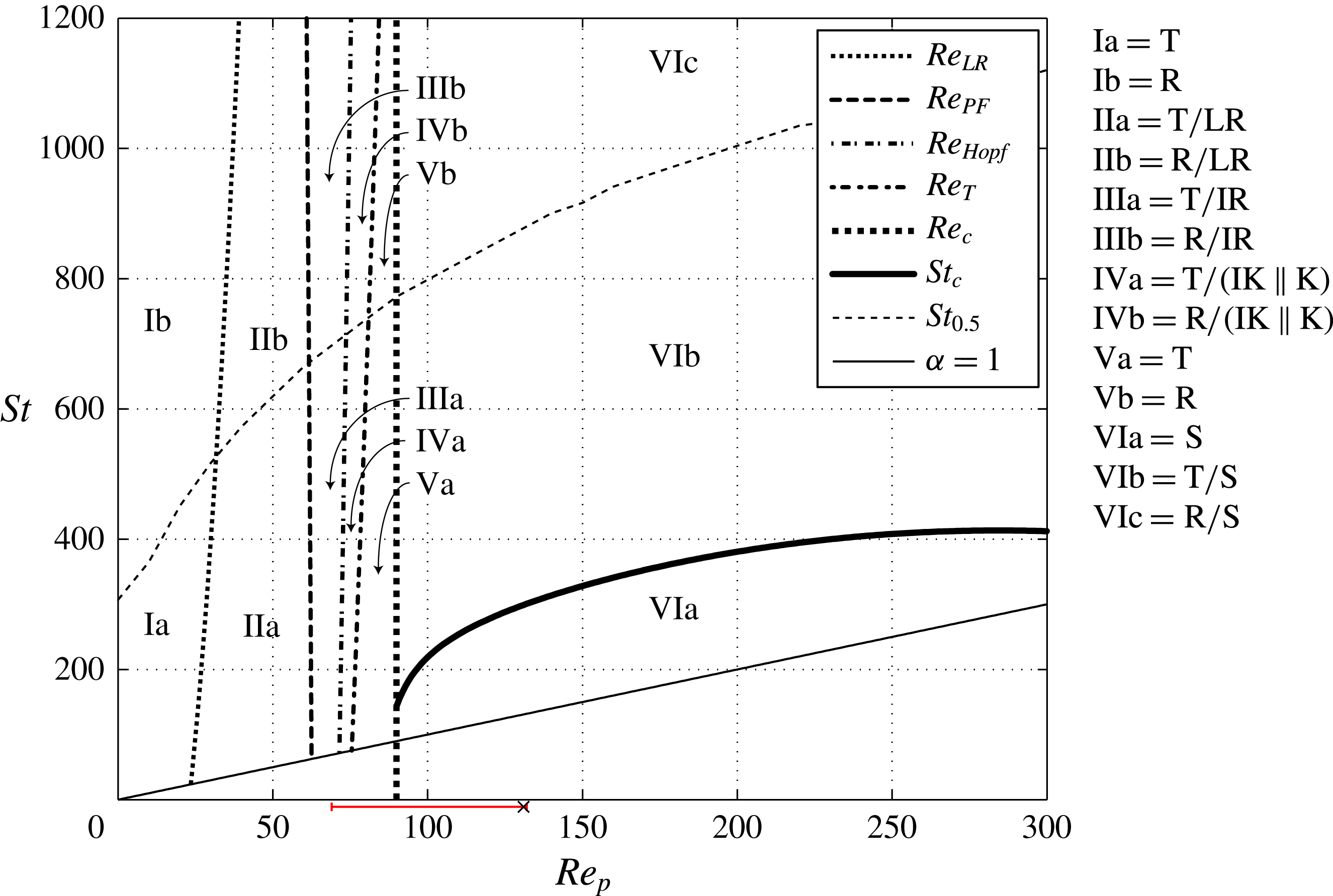
Regime Ia (
$\mathit{Re}_{p}<\mathit{Re}_{\mathit{LR}}$
and
$\mathit{St}<\mathit{St}_{0.5}$
)


All initial conditions lead to tumbling.
Regime Ib (
$\mathit{Re}_{p}<\mathit{Re}_{\mathit{LR}}$
and
$\mathit{St}>\mathit{St}_{0.5}$
)


All initial conditions lead to rotating.
Regime IIa (
$\mathit{Re}_{\mathit{LR}}<\mathit{Re}_{p}<\mathit{Re}_{PF}$
and
$\mathit{St}<\mathit{St}_{0.5}$
)


Tumbling and log-rolling are stable solutions; the final state depends on the initial conditions.
Regime IIb (
$\mathit{Re}_{\mathit{LR}}<\mathit{Re}_{p}<\mathit{Re}_{PF}$
and
$\mathit{St}>\mathit{St}_{0.5}$
)


Rotating and log-rolling are stable solutions; the final state depends on the initial conditions.
Regime IIIa (
$\mathit{Re}_{PF}<\mathit{Re}_{p}<\mathit{Re}_{\mathit{Hopf}}$
and
$\mathit{St}<\mathit{St}_{0.5}$
)


Tumbling and inclined rolling are stable solutions; the final state depends on the initial conditions.
Regime IIIb (
$\mathit{Re}_{PF}<\mathit{Re}_{p}<\mathit{Re}_{\mathit{Hopf}}$
and
$\mathit{St}>\mathit{St}_{0.5}$
)


Rotating and inclined rolling are stable solutions; the final state depends on the initial conditions.
Regime IVa (
$\mathit{Re}_{\mathit{Hopf}}<\mathit{Re}_{p}<\mathit{Re}_{T}$
and
$\mathit{St}<\mathit{St}_{0.5}$
)


Tumbling and inclined kayaking (and kayaking when the inclined kayaking solutions merge) are stable solutions; the final state depends on the initial conditions.
Regime IVb (
$\mathit{Re}_{\mathit{Hopf}}<\mathit{Re}_{p}<\mathit{Re}_{T}$
and
$\mathit{St}>\mathit{St}_{0.5}$
)


Rotating and inclined kayaking (and kayaking when the inclined kayaking solutions merge) are stable solutions; the final state depends on the initial conditions.
Regime Va (
$\mathit{Re}_{T}<\mathit{Re}_{p}<\mathit{Re}_{c}$
and
$\mathit{St}<\mathit{St}_{0.5}$
)


All initial conditions lead to tumbling.
Regime Vb (
$\mathit{Re}_{T}<\mathit{Re}_{p}<\mathit{Re}_{c}$
and
$\mathit{St}>\mathit{St}_{0.5}$
)


All initial conditions lead to rotating.
Regime VIa (
$\mathit{Re}_{p}>\mathit{Re}_{c}$
and
$\mathit{St}<\mathit{St}_{c}$
)


All initial conditions lead to steady state.
Regime VIb (
$\mathit{Re}_{p}>\mathit{Re}_{c}$
and
$\mathit{St}_{c}<\mathit{St}<\mathit{St}_{0.5}$
)


Tumbling and steady state are stable solutions; the final state depends on the initial conditions.
Regime VIc (
$\mathit{Re}_{p}>\mathit{Re}_{c}$
and
$\mathit{St}_{c}<\mathit{St}<\mathit{St}_{0.5}$
)


Rotating and steady state are stable solutions; the final state depends on the initial conditions.
The methods used to determine the curves in figure 11 will now be described in detail.
4.4. Determining
$\mathit{St}_{c}$
as function of
$\mathit{Re}_{p}$


4.4.1. Definition of
$\mathit{St}_{c}$

As already shown, the saddle-node bifurcation at
 $\mathit{Re}_{p}=\mathit{Re}_{c}$
gives rise to two equilibrium orientations, at which there is zero torque on the particle: one stable orientation,
 ${\it\phi}_{c}$
, and one unstable orientation,
 ${\it\phi}_{us}$
(see figure 5). This means that for a small deviation
 ${\it\phi}_{c}\pm {\it\delta}{\it\phi}$
or
 ${\it\phi}_{us}+{\it\delta}{\it\phi}$
, the particle will go to
 ${\it\phi}_{c}$
, but a small negative deviation
 ${\it\phi}_{us}-{\it\delta}{\it\phi}$
will make the particle rotate around the vorticity direction until it is almost aligned with the flow again at
 ${\it\phi}_{c}-{\rm\pi}$
. If the particle has enough particle inertia, it will gain enough angular momentum during the rotation that the region of positive torque will be insufficient to stop the rotation. The particle will thus reach the symmetric (and dynamically identical) configuration
 ${\it\phi}_{us}-{\rm\pi}$
with a non-zero angular velocity and consequently enter a periodic tumbling motion. This leads to a natural definition of a critical Stokes number
 $\mathit{St}_{c}$
: when initializing the particle at rest at an angle
 ${\it\phi}_{us}-{\it\delta}{\it\phi}$
, a particle with
 $\mathit{St}<\mathit{St}_{c}$
will end up in steady state whereas a particle with
 $\mathit{St}>\mathit{St}_{c}$
will end up in a tumbling motion.
Below
 $\mathit{St}_{c}$
, all initial conditions will lead to the steady state, since the particle can never gain more angular momentum during a rotational period. So even if the particle is initialized with high angular velocity, it will eventually slow down until it reaches a steady state. Above
 $\mathit{St}_{c}$
, the final solution can be either tumbling motion or steady state, depending on the initial condition. As will be shown in § 5, the transition from tumbling to steady state at
 $\mathit{St}=\mathit{St}_{c}$
is through a homoclinic bifurcation. The critical Stokes number is determined by finding the critical density ratio
 ${\it\alpha}_{c}=\mathit{St}_{c}/\mathit{Re}_{p}$
as a function of
 $\mathit{Re}_{p}$
.
4.4.2. Equilibrium angles
In order to find the critical density ratio
 ${\it\alpha}_{c}$
, the equilibrium angle
 ${\it\phi}_{us}$
must be found. Both
 ${\it\phi}_{us}$
and
 ${\it\phi}_{c}$
are found by using the fact that there should be zero torque on the particle, which means that
 $\dot{{\it\phi}}\approx 0$
should be achieved shortly after the particle is initialized in an equilibrium angle. This fact is used to systematically find the equilibrium angles for a given
 $\mathit{Re}_{p}$
with a half-interval search (the exact algorithm is described in appendix B).
In figure 12,
 ${\it\phi}_{c}$
and
 ${\it\phi}_{us}$
are plotted as functions of
 $\mathit{Re}_{p}$
. It can be seen that
 ${\it\phi}_{us}$
and
 ${\it\phi}_{c}$
are decreasing and increasing functions of
 $\mathit{Re}_{p}$
, respectively. A seventh-order polynomial is fitted to the computed data points, and using the polynomial function the bifurcation is found to occur at
 $\mathit{Re}_{c}\approx 90$
, which is slightly higher than the previously obtained value of
 $\mathit{Re}_{c}\approx 89$
.
Equilibrium angles
 ${\it\phi}_{c}$
(circles) and
 ${\it\phi}_{us}$
(crosses) plotted as functions of
 $\mathit{Re}_{p}$
for a spheroid with
 $r_{p}=4$
; the data are fitted with a polynomial function (solid line), for which the minimum is found at
 $\mathit{Re}_{p}=\mathit{Re}_{c}=90$
.

4.4.3. Critical density ratio as a function of
$\mathit{Re}_{p}$

The critical density ratio,
 ${\it\alpha}_{c}$
, is obtained as described in § 4.4.1, with
 ${\it\delta}{\it\phi}$
chosen sufficiently large so that the particle is definitely moving with
 $\dot{{\it\phi}}<0$
. In this study,
 ${\it\delta}{\it\phi}$
was chosen to be
 $1^{\circ }$
. The critical density ratio
 ${\it\alpha}_{c}$
is found by using the fact that the particle with
 ${\it\alpha}={\it\alpha}_{c}$
initialized at rest from
 ${\it\phi}_{0}={\it\phi}_{us}-{\it\delta}{\it\phi}$
should reach
 ${\it\phi}={\it\phi}_{0}-{\rm\pi}$
with
 $\dot{{\it\phi}}=0$
. The critical density ratio is found by using half-interval search (the exact algorithm is provided in appendix C).
Figure 13 shows
 ${\it\alpha}_{c}$
as a function of
 $\mathit{Re}_{p}$
, where the data points are fitted with a rational function of the form
 ${\it\alpha}_{c}=P(\mathit{Re}_{p})/Q(\mathit{Re}_{p})$
, with
 $P$
and
 $Q$
being fifth- and fourth-degree polynomials, respectively. The error bars indicate the minimum intervals
 ${\rm\Delta}\mathit{St}=10$
used in the half-interval algorithm. The maximum critical density ratio of
 ${\it\alpha}_{c,max}\approx 2.3$
is found close to
 $\mathit{Re}_{p}\approx 125$
, while at higher
 $\mathit{Re}_{p}$
particle inertia plays a greater role and
 ${\it\alpha}$
does not need to be much larger than unity in order to find a periodic state. It can also be seen from the figure that
 ${\it\alpha}_{c}>1$
as
 $\mathit{Re}_{p}=\mathit{Re}_{c}$
. This codimension-two point
 ${\it\alpha}_{cd2}={\it\alpha}_{c}(\mathit{Re}_{c})\approx 1.6$
, where two bifurcations coexist (the saddle-node bifurcaction at
 $\mathit{Re}_{c}$
and the homoclinic bifurcation at
 ${\it\alpha}_{c}$
), is found by evaluating the fitted rational function at
 $\mathit{Re}_{c}$
. A more detailed discussion of this bifurcation will be given in § 5. The line of
 $\mathit{St}_{c}$
in figure 11 is drawn by the relation
 $\mathit{St}_{c}={\it\alpha}_{c}\,\mathit{Re}_{p}$
, which connects to the codimension-two point at
 $\mathit{St}_{cd2}={\it\alpha}_{cd2}\mathit{Re}_{c}$
.
The critical density ratio
 ${\it\alpha}_{c}$
plotted as a function of
 $\mathit{Re}_{p}$
for a spheroid with
 $r_{p}=4$
(solid blue line), fitted with a rational function (solid black line). The critical Reynolds number
 $\mathit{Re}_{c}=90$
(dashed line) is found through polynomial fitting of equilibrium angles, and the codimension-two point, where
 ${\it\alpha}_{c}$
connects to the
 $\mathit{Re}_{c}$
line, is found at
 ${\it\alpha}={\it\alpha}_{cd2}\approx 1.6$
. Black crosses indicate
 ${\it\alpha}=2,2.5$
and 3 at
 $\mathit{Re}_{p}=150$
, for which the phase diagrams in figure 14 are drawn. Only planar rotational states, namely tumbling (T) and steady state (S), are shown in the figure.

4.5. Determining
$\mathit{St}_{0.5}$
as function of
$\mathit{Re}_{p}$


As already discussed, it was observed by Lundell & Carlsson (Reference Lundell and Carlsson2010) and Nilsen & Andersson (Reference Nilsen and Andersson2013) that the period of the tumbling motion is a steadily decreasing function of
 $\mathit{St}$
in the absence of fluid inertia (
 $\mathit{Re}_{p}=0$
). At
 $\mathit{St}=0$
, the particle is tumbling with period
 $GT_{J}=2{\rm\pi}(r_{p}^{-1}+r_{p})$
; as
 $\mathit{St}\rightarrow \infty$
, the particle rotates at a constant angular velocity with period
 $GT_{H}=4{\rm\pi}$
. The transition between the two regimes is characterized by
 $\mathit{St}_{0.5}$
, which is defined as the Stokes number at which the spheroid rotates with a period of
 $(GT_{J}+GT_{H})/2$
. However,
 $\mathit{St}_{0.5}$
was defined only for
 $\mathit{Re}_{p}=0$
, since it refers to the period without any fluid or particle inertia. For finite
 $\mathit{Re}_{p}>0$
, the period is also seen to decrease as
 $\mathit{St}$
increases; therefore in this work we use the same definition of
 $\mathit{St}_{0.5}$
, i.e. the Stokes number at which the period is
 $GT=(GT_{J}+GT_{H})/2={\rm\pi}(r_{p}^{-1}+r_{p}+2)$
. The value of
 $\mathit{St}_{0.5}$
is found by using a half-interval search (see appendix D for the exact algorithm). Since the value at
 $\mathit{Re}_{p}=0$
can be analytically found to be
 $\mathit{St}_{0.5}=307$
, the line with the simulated values has been connected to this analytical value in figure 11.
4.6. Determining
$\mathit{Re}_{\mathit{LR}},\mathit{Re}_{PF},\mathit{Re}_{\mathit{Hopf}}$
and
$\mathit{Re}_{T}$
as functions of
$\mathit{St}$



4.6.1.
$\mathit{Re}_{\mathit{LR}}$

The definition of
 $\mathit{Re}_{\mathit{LR}}$
is as the value at which the log-rolling solution goes from being unstable, with outward-spiralling trajectories, to stable, with nearby trajectories spiralling inwards. In the work by Rosén et al. (Reference Rosén, Lundell and Aidun2014), this value was determined by initializing a particle in the log-rolling solution and observing whether it was still there after a certain length of time or if it had started to spiral outwards. In this work, for better comparison with the heavier particle, we make use of the fact that the log-rolling solution should become attracting at
 $\mathit{Re}_{\mathit{LR}}$
. Therefore, a particle is initialized at rest from a nearby location at
 $({\it\phi},{\it\theta})=(0^{\circ },1^{\circ })$
, and the
 $\mathit{Re}_{p}$
value at which this initial condition leads to log-rolling instead of tumbling is taken to be
 $\mathit{Re}_{\mathit{LR}}$
. This is done for both a neutrally buoyant particle and a particle with
 ${\it\alpha}=20$
.
The value of
 $\mathit{Re}_{\mathit{LR}}$
increases to
 $\mathit{Re}_{\mathit{LR}}\approx 33.5$
from
 $\mathit{Re}_{\mathit{LR}}\approx 23.5$
as
 ${\it\alpha}$
is increased from 1 to 20 (note that, with this definition, the value of
 $\mathit{Re}_{\mathit{LR}}$
for the neutrally buoyant case is slightly higher than the value reported by Rosén et al. (Reference Rosén, Lundell and Aidun2014)). With high
 ${\it\alpha}$
, small disturbances of the particle orientation will lead to a more considerable gain in angular momentum and an increased influence of particle inertia effects. Therefore, the transition that stabilizes the log-rolling solution is delayed in
 $\mathit{Re}_{p}$
as
 ${\it\alpha}$
is increased.
4.6.2.
$\mathit{Re}_{PF}$

The transition at
 $\mathit{Re}_{PF}$
is associated with the fact that the log-rolling solution destabilizes and the particle ends up in inclined rolling with
 ${\it\theta}>0$
. The value of
 $\mathit{Re}_{PF}$
is determined by finding the
 $\mathit{Re}_{p}$
value at which a particle initialized close to the log-rolling solution at
 $({\it\phi},{\it\theta})=(0^{\circ },1^{\circ })$
ends up with an angle
 ${\it\theta}>1^{\circ }$
after
 $Gt=400$
. This is done both for a neutrally buoyant particle and for a particle with
 ${\it\alpha}=13$
.
For the neutrally buoyant particle, the transition was found to occur at
 $\mathit{Re}_{PF}=62.5$
, and the heavy particle had a transition at
 $\mathit{Re}_{PF}=61.5$
. The transition point appears not to change for higher
 ${\it\alpha}$
, and the reason for the small variation in
 $\mathit{Re}_{PF}$
is that the heavier particle assumes the final rotational state more quickly than the lighter one. The alignment to the new inclined rolling state is very slow, and so particle inertia is concluded to be negligible for this transition. This can be understood by recalling that both the log-rolling and inclined rolling solutions correspond to steady states of the fluid field.
4.6.3.
$\mathit{Re}_{\mathit{Hopf}}$

The transition at
 $\mathit{Re}_{\mathit{Hopf}}$
is associated with a final rotational state where
 ${\it\theta}$
goes from being a constant to an oscillating function of time. To determine
 $\mathit{Re}_{\mathit{Hopf}}$
, we use the fact that a particle with an initial orientation of
 $({\it\phi},{\it\theta})=(0,{\rm\pi}/8)$
will quickly enter the final rotational state close to
 $\mathit{Re}_{\mathit{Hopf}}$
(this can be seen in figure 4
e for initial orientation 2). The
 $\mathit{Re}_{p}$
value at which the oscillations of this particle become larger than
 ${\rm\Delta}{\it\theta}=1^{\circ }$
after
 $Gt=1000$
is taken to be
 $\mathit{Re}_{\mathit{Hopf}}$
. This is simulated for both
 ${\it\alpha}=1$
and
 ${\it\alpha}=13$
.
For the transition at
 $\mathit{Re}_{\mathit{Hopf}}$
, particle inertia plays a role, but small disturbances do not affect the particle that much. Most likely because of this,
 $\mathit{Re}_{\mathit{Hopf}}$
increases slightly from
 $\mathit{Re}_{\mathit{Hopf}}\approx 71.5$
to
 $\mathit{Re}_{\mathit{Hopf}}\approx 73.5$
as
 ${\it\alpha}$
is increased from 1 to 13.
4.6.4.
$\mathit{Re}_{T}$

The transition at
 $\mathit{Re}_{T}$
is associated with a final rotational state that is tumbling regardless of the initial orientation. Here
 $\mathit{Re}_{T}$
is defined as the
 $\mathit{Re}_{p}$
value at which a particle initialized at
 $({\it\phi},{\it\theta})=(0,0)$
spirals outward towards a tumbling motion after
 $Gt=400$
. This is investigated both for a light particle (
 ${\it\alpha}=1$
) and a heavy particle (
 ${\it\alpha}=13$
).
A bigger difference is seen for this transition than for the previous ones. The oscillations of the heavier particle in the inclined kayaking state have smaller amplitude due to lower angular acceleration. This leads to a delayed transition to the pure tumbling region from
 $\mathit{Re}_{T}\approx 75.5$
for
 ${\it\alpha}=1$
to
 $\mathit{Re}_{T}\approx 83.5$
for
 ${\it\alpha}=13$
.
In figure 11, the dependence of
 $\mathit{Re}_{\mathit{LR}}$
,
 $\mathit{Re}_{\mathit{Hopf}}$
and
 $\mathit{Re}_{T}$
on the solid-to-fluid density ratio
 ${\it\alpha}$
is estimated by linearly interpolating the two results at low
 ${\it\alpha}$
and at high
 ${\it\alpha}$
given above. The curves therefore take on a slightly parabolic shape, as they are drawn according to the relation
 $\mathit{St}={\it\alpha}\,\mathit{Re}_{p}$
for
 $\mathit{Re}_{\mathit{LR}}$
,
 $\mathit{Re}_{PF}$
,
 $\mathit{Re}_{\mathit{Hopf}}$
and
 $\mathit{Re}_{T}$
.
The Stokes number is seen to have a small or no effect on the transitions at
 $\mathit{Re}_{\mathit{LR}}$
,
 $\mathit{Re}_{PF}$
,
 $\mathit{Re}_{\mathit{Hopf}}$
and
 $\mathit{Re}_{T}$
, and we conclude that particle inertia has little effect due to the slow non-planar motions. These transitions are thus mainly controlled by fluid inertia.
5. Results: bifurcation analysis
$(r_{p}=4)$

In this section we discuss the results on the spheroid in a shear flow using general theory about nonlinear dynamical systems and bifurcations. The concepts discussed can be found in the books by Hale & Koçak (Reference Hale and Koçak1991) and Strogatz (Reference Strogatz1994).
5.1. Bifurcation at
${\it\alpha}={\it\alpha}_{c}~(St=\mathit{St}_{c})$

From figure 13 it can be seen that for a particle of
 ${\it\alpha}>{\it\alpha}_{c,max}$
, fluid inertia will never be enough to fully stop a tumbling motion, and there will be no diverging period when
 $\mathit{Re}_{p}$
increases or decreases (a steady state will still always coexist at
 $\mathit{Re}_{p}>\mathit{Re}_{c}$
). However, by fixing
 $\mathit{Re}_{p}>\mathit{Re}_{c}$
and decreasing
 ${\it\alpha}$
, the period diverges at
 ${\it\alpha}={\it\alpha}_{c}$
. This transition is not the infinite-period saddle-node bifurcation seen at
 $\mathit{Re}_{p}=\mathit{Re}_{c}$
, since no new fixed points are created. To understand this process, phase diagrams of the motion are drawn in figure 14(b–d), where a particle is initialized at rest from eight different initial orientations,
 $({\it\phi},{\it\theta})_{1{-}8}=({\rm\pi}n/8,{\rm\pi}/2)$
for
 $n=0,1,\dots ,7$
(see figure 14
a), at
 $\mathit{Re}_{p}=150$
and three different density ratios
 ${\it\alpha}=2,2.5$
and 3 (crosses in figure 13). As shown in figure 12, the equilibrium angles at
 $\mathit{Re}_{p}=150$
are
 ${\it\phi}_{us}\approx 0^{\circ }$
and
 ${\it\phi}_{c}\approx 15.5^{\circ }$
.
Phase diagrams showing homoclinic bifurcation for a spheroid with
 $r_{p}=4$
at
 $\mathit{Re}_{p}=150$
, initialized at rest in the flow-gradient plane (
 ${\it\theta}=90^{\circ }$
) from eight different initial orientations, shown in (a), and with three different density ratios: (b)
 ${\it\alpha}=3$
; (c)
 ${\it\alpha}=2.5$
; (d)
 ${\it\alpha}=2$
. A limit cycle (tumbling) is seen to collapse with the saddle
 ${\it\phi}_{us}$
(open circle) at
 ${\it\alpha}={\it\alpha}_{c}=2.2$
; at
 ${\it\alpha}<{\it\alpha}_{c}$
, all initial conditions lead to the sink
 ${\it\phi}_{c}$
(solid circle) and thus stay in steady state.

Starting with the case where
 ${\it\alpha}=3$
in figure 14(b), the point at
 $(\dot{{\it\phi}},{\it\phi})=(0,{\it\phi}_{us})$
is a saddle (open circle, with stable dynamics in one eigendirection and unstable dynamics in another eigendirection) while
 $(\dot{{\it\phi}},{\it\phi})=(0,{\it\phi}_{c})$
is a sink (filled circle, with stable dynamics, i.e. nearby trajectories go to this point). The trajectory of the initial condition
 ${\it\phi}_{1}$
almost coincides with the saddle (i.e.
 ${\it\phi}_{1}={\it\phi}_{us}$
) and can be considered a branch of the unstable manifold of the saddle. This manifold asymptotically approaches the stable limit cycle, i.e. a tumbling motion. At some trajectory between the trajectories of initial conditions
 ${\it\phi}_{6}$
and
 ${\it\phi}_{7}$
, there is a branch of the stable manifold of the saddle; this means that initial conditions above it (e.g. initial conditions 2–6) lead to the sink, i.e. steady state. As
 ${\it\alpha}$
is decreased close to
 ${\it\alpha}_{c}$
, the stable limit cycle goes very near the saddle, as seen in figure 14(c). At
 ${\it\alpha}={\it\alpha}_{c}\approx 2.2$
, the stable limit cycle is destroyed as the limit cycle merges with the unstable manifold of the saddle. The manifold becomes a homoclinic orbit which connects with itself at the saddle. At
 ${\it\alpha}<{\it\alpha}_{c}$
, even the unstable manifold of the saddle leads to the sink and therefore the steady state is the only solution (figure 14
d).
The behaviour is very similar to that of a damped pendulum driven by a constant torque (Strogatz Reference Strogatz1994), which undergoes a homoclinic bifurcation when the driving torque is varied under low damping conditions. The period of the limit cycle is divergent, but unlike the case of an infinite-period saddle-node bifurcation, where the period scales as
 $GT\propto |{\it\beta}-{\it\beta}_{c}|^{-0.5}$
, the period close to the homoclinic bifurcation scales as
 $GT\propto \ln |{\it\beta}-{\it\beta}_{c}|$
, where
 ${\it\beta}$
is any parameter leading to the transition at
 ${\it\beta}_{c}$
. In figure 15(a,b), the period is plotted as a function of
 ${\it\alpha}-{\it\alpha}_{c}$
and is compared with the two types of scaling at
 $\mathit{Re}_{p}=150$
. It is clear that the logarithmic scaling gives a much better fit, and the existence of a homoclinic bifurcation at
 ${\it\alpha}={\it\alpha}_{c}$
is confirmed. The reason that the power law fails to describe the diverging period in this case is that the angular velocity becomes a non-differentiable function of the angle close to the saddle (seen also in figure 13
b), which is an important criterion for this scaling (Strogatz Reference Strogatz1994; Rosén et al.
Reference Rosén, Lundell and Aidun2014). The shape of
 $\dot{{\it\phi}}({\it\phi})$
close to
 ${\it\phi}_{us}$
is determined by the two eigendirections of the saddle when
 ${\it\alpha}\gtrsim {\it\alpha}_{c}$
and therefore has a non-parabolic shape.
Scaling of the diverging period at
 $\mathit{Re}_{p}=150$
for a spheroid with
 $r_{p}=4$
: (a) data fitted using the assumption of a homoclinic bifurcation with
 $GT\propto \ln |{\it\beta}-{\it\beta}_{c}|$
; (b) data fitted using the assumption of an infinite-period saddle-node bifurcation with
 $GT\propto |{\it\beta}-{\it\beta}_{c}|^{-0.5}$
.

Combining this knowledge with what was found regarding the coexistence of the tumbling solution and a steady state (figure 13), the following conclusions can be drawn for a prolate spheroid of aspect ratio
 $r_{p}=4$
with increasing
 $\mathit{Re}_{p}$
.
-
(i) If
${\it\alpha}<{\it\alpha}_{cd2}\approx 1.6$
, the transition from tumbling to steady state will be through an infinite-period saddle-node bifurcation at
$\mathit{Re}_{p}=\mathit{Re}_{c}$
, with a diverging period scaling as
$GT\propto |\mathit{Re}_{p}-\mathit{Re}_{c}|^{-0.5}$
. -
(ii) If
${\it\alpha}_{cd2}<{\it\alpha}<{\it\alpha}_{c,max}$
(i.e.
$1.6\lesssim {\it\alpha}\lesssim 2.3$
), the transition will be through a homoclinic bifurcation at
$\mathit{Re}_{p}=\mathit{Re}_{c1}$
, where
$\mathit{Re}_{c1}$
is defined as the
$\mathit{Re}_{p}$
value at which
${\it\alpha}={\it\alpha}_{c}$
. The tumbling period will diverge according to
$GT\propto \ln |\mathit{Re}_{p}-\mathit{Re}_{c1}|$
. -
(iii) If
${\it\alpha}={\it\alpha}_{cd2}\approx 1.6$
, a transition from tumbling to steady state will occur at
$\mathit{Re}_{p}=\mathit{Re}_{c}$
, but no distinction can be made between the types of bifurcations and both types of scalings will apply. -
(iv) If
${\it\alpha}>{\it\alpha}_{c,max}\approx 2.3$
, there is no diverging period at any
$\mathit{Re}_{p}$
, and a tumbling solution will always exist.









5.2. Bifurcation diagrams
The bifurcation diagrams for
 ${\it\alpha}=2$
and 3 are shown in figure 16(a,b) in the same way as in § 3.3. Looking at figure 16(a), for
 ${\it\alpha}=2$
, which lies in the interval
 ${\it\alpha}_{cd2}<{\it\alpha}<{\it\alpha}_{c,max}$
, there are two critical particle Reynolds numbers which correspond to intersections of the
 ${\it\alpha}_{c}$
line (see figure 13). Due to higher particle inertia, the fluid inertia is not sufficient to stop the tumbling motion at
 $\mathit{Re}_{p}=\mathit{Re}_{c}$
(note that
 $\mathit{Re}_{c}$
is dependent only on geometry and fluid properties and is not changed due to high particle inertia). The tumbling period instead diverges to infinity at
 $\mathit{Re}_{p}=\mathit{Re}_{c1}>\mathit{Re}_{c}$
through a homoclinic bifurcation. Similar behaviour is seen when
 $\mathit{Re}_{p}$
is decreased from high values, with the tumbling period diverging to infinity at
 $\mathit{Re}_{c2}$
. In the region
 $\mathit{Re}_{c1}<\mathit{Re}_{p}<\mathit{Re}_{c2}$
, the steady state is thus the only solution, while a tumbling solution coexists in the regions
 $\mathit{Re}_{c}<\mathit{Re}_{p}<\mathit{Re}_{c1}$
and
 $\mathit{Re}_{p}>\mathit{Re}_{c2}$
. For the particle with
 ${\it\alpha}=3$
(figure 16
b), the density ratio is higher than
 ${\it\alpha}_{c,max}$
, and hence there is no diverging period and a tumbling solution will always coexist with the steady state at
 $\mathit{Re}_{p}>\mathit{Re}_{c}$
. The bifurcation diagrams indicate the following hysteresis behaviour as
 $\mathit{Re}_{p}$
varies.
-
(i) For a particle with
${\it\alpha}_{cd2}<{\it\alpha}<{\it\alpha}_{c,max}$
(figure 16
a) in a tumbling state at
$\mathit{Re}_{p}<\mathit{Re}_{c}$
, increasing
$\mathit{Re}_{p}$
will lead to a diverging period and a transition to steady state at
$\mathit{Re}_{p}=\mathit{Re}_{c1}$
. However, to reach a tumbling state again,
$\mathit{Re}_{p}$
must be decreased to
$\mathit{Re}_{p}=\mathit{Re}_{c}$
, since the steady-state solution (bold line at
$N_{C}=1$
) exists also for
$\mathit{Re}_{c}<\mathit{Re}_{p}<\mathit{Re}_{c1}$
. -
(ii) For a particle with
${\it\alpha}<{\it\alpha}_{c,max}$
(figure 16
a) in a tumbling state at
$\mathit{Re}_{p}>\mathit{Re}_{c2}$
, decreasing
$\mathit{Re}_{p}$
will lead to a diverging period and a transition to steady state at
$\mathit{Re}_{p}=\mathit{Re}_{c2}$
. Upon increasing
$\mathit{Re}_{p}>\mathit{Re}_{c2}$
, the particle will stay in steady state. -
(iii) For a particle with
${\it\alpha}>{\it\alpha}_{c,max}$
(figure 16
b) in a steady state, decreasing
$\mathit{Re}_{p}$
past
$\mathit{Re}_{c}$
will make the particle enter a tumbling motion. If
$\mathit{Re}_{p}$
is increased again, the particle will stay in a tumbling rotational state.





Bifurcation diagrams for a spheroid of
 $r_{p}=4$
with: (a)
 ${\it\alpha}=2$
; (b)
 ${\it\alpha}=3$
. In each panel, the zoomed-in region for
 $\mathit{Re}_{p}$
between 60 and 100 is displayed on the right; the stable rotational states have either a fixed orientation (solid lines) or an oscillating orientation (grey areas), where in the latter case the norm is plotted using
 $N_{C,max}$
and
 $N_{C,min}$
during an oscillation period. The unstable fixed points are schematically drawn with dashed lines, and the approximate location of
 $N_{max}$
for the unstable limit cycle is indicated by open circles.

6. Results: transient behaviour and orbit drift (
$r_{p}=4$
)

Although we saw in § 4.6 that the transitions at
 $\mathit{Re}_{\mathit{LR}},\mathit{Re}_{PF},\mathit{Re}_{\mathit{Hopf}}$
and
 $\mathit{Re}_{T}$
are not affected much by
 ${\it\alpha}$
, a significant difference emerges when one studies the rate at which the particle assumes an equilibrium solution. Figure 17(a,b) show the projected trajectories of a particle with
 ${\it\alpha}=13$
at
 $\mathit{Re}_{p}=60$
and
 $\mathit{Re}_{p}=70$
, respectively, for the initial orientations given by (3.1). Compared with the neutrally buoyant particle in figure 4(b,c), the unstable orbit appears unchanged, leading to a similar probability that a randomly oriented particle initialized at rest will end up in each rotational state. However, the oscillations of the particle orientation are almost completely damped out by particle inertia. The evolution of the
 ${\it\theta}$
angle for the heavy particle is shown in figures 17(c) and 4(d) for
 $\mathit{Re}_{p}=60$
and 70, respectively. It is obvious that, although the final rotational state remains unchanged when the density ratio is altered, the rate of approach to the final state is strongly affected. In the range of
 $\mathit{St}$
studied here, the heavier particle always reaches the final rotational state more rapidly than does a lighter particle. However, as observed by Lundell & Carlsson (Reference Lundell and Carlsson2010) for
 $\mathit{Re}_{p}=0$
, at higher
 $\mathit{Re}_{p}$
there is probably also an optimal Stokes number, above which the rate of reaching the final state increases instead, due to a slow initial transient.
Projected trajectories of a heavy particle with
 $r_{p}=4$
and
 ${\it\alpha}=13$
at: (a)
 $\mathit{Re}_{p}=60$
(T/LR); (b)
 $\mathit{Re}_{p}=70$
(T/IR). The bottom panels show the evolution of the particle orientation (with just the
 ${\it\theta}$
angle plotted) for the heavy particle (solid line) compared with that of a neutrally buoyant particle (dashed line); the projected trajectories are as presented earlier in figure 4.
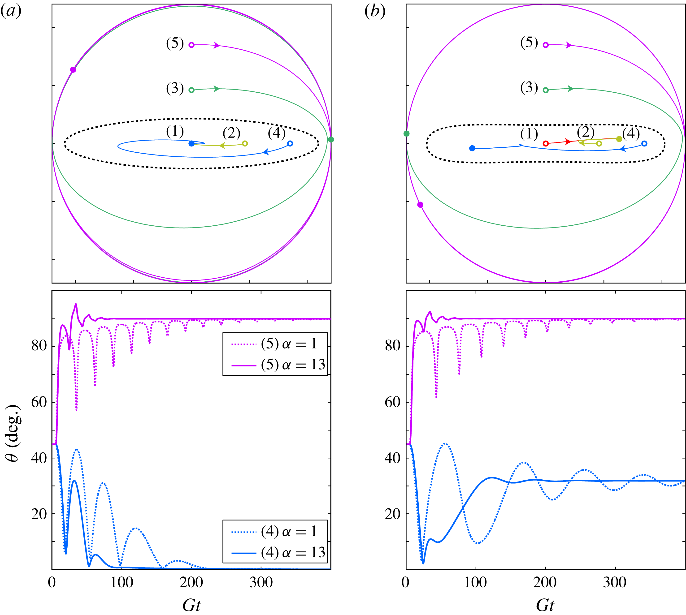
Intrinsic viscosity of one-particle suspension (
 $r_{p}=4$
) as a function of
 $\mathit{Re}_{p}$
for
 ${\it\alpha}=1$
(thick lines in main plot) and
 ${\it\alpha}=2,2.2,2.5,3,4,5$
(thin lines in main plot); the dashed line connects the analytical value of
 ${\it\eta}$
of the tumbling motion derived at
 $\mathit{Re}_{p}=0$
by Jeffery (Reference Jeffery1922) to the first simulated value at
 $\mathit{Re}_{p}=10$
, since it is known that this is the only stable rotational state in the low-
 $\mathit{Re}_{p}$
regime. The inset shows the corresponding parameter sweep in the
 $\mathit{Re}_{p}$
–
 $\mathit{St}$
plane. Here
 $\text{T}=\text{tumbling}$
(black lines in main plot),
 $\text{S}=\text{steady}$
state (yellow),
 $\text{LR}=\text{log-rolling}$
(red) and
 $\text{IR}=\text{inclined}$
rolling (cyan); for simplicity, the rotational states of inclined kayaking and kayaking are included in the inclined rolling regime.

7. Results: consequences for suspension rheology
One of the key consequences of the preferred rotational states due to inertia is the effect on the rheological properties of the particle suspension. Einstein (Reference Einstein1906, Reference Einstein1911) already found that the shear viscosity of a dilute suspension
 ${\it\nu}_{susp}$
of spherical particles is modified through a relation
 ${\it\nu}_{susp}={\it\nu}(1+{\it\eta}{\it\Phi})$
, where
 ${\it\nu}$
is the kinematic viscosity of the suspending fluid,
 ${\it\Phi}$
is the particle volume fraction and
 ${\it\eta}$
is the intrinsic viscosity. For a suspension of spherical particles, the intrinsic viscosity was found to be
 ${\it\eta}=2.5$
. Jeffery (Reference Jeffery1922) extended this work to account for spheroids, and found that
 ${\it\eta}$
depends on the rotational orbit. For an inertia-less prolate spheroid with
 $r_{p}=4$
, the intrinsic viscosity averaged over a full period has a value ranging from
 ${\it\eta}_{Jeffery}\approx 2.05$
(in the log-rolling orbit) to
 ${\it\eta}_{Jeffery}\approx 3.36$
(in the tumbling orbit). In the work by Huang et al. (Reference Huang, Wu and Lu2012a
,Reference Huang, Yang, Krafczyk and Lu
b
) using a lattice Boltzmann method,
 ${\it\eta}$
was found by evaluating the shear stress
 ${\it\sigma}$
at the fluid nodes closest to the wall. The same method is employed here for each final rotational state at different values of
 $\mathit{Re}_{p}$
and
 ${\it\alpha}$
(the method is described in detail in appendix E). The results are shown in figure 18. If we consider a constant fluid viscosity and constant particle size, the
 $\mathit{Re}_{p}$
-axis can be interpreted as the shear rate. Both shear-thinning (
 $\text{d}{\it\eta}/\text{d}\mathit{Re}_{p}<0$
) and shear-thickening (
 $\text{d}{\it\eta}/\text{d}\mathit{Re}_{p}>0$
) can thus be directly deduced from the diagram. The thick lines correspond to the neutrally buoyant case and show a shear-thickening behaviour everywhere except in a small region just below
 $\mathit{Re}_{p}=\mathit{Re}_{c}$
, where the diverging period, due to the infinite-period saddle-node bifurcation, causes shear-thinning. In the
 $\mathit{Re}_{\mathit{LR}}<\mathit{Re}_{p}<\mathit{Re}_{T}$
regime, two values of
 ${\it\eta}$
are allowed, since we have coexisting rotational states corresponding to planar and non-planar motions. When
 ${\it\alpha}>{\it\alpha}_{c,max}$
, the diverging period disappears and so does the small shear-thinning region, and the suspension has shear-thickening behaviour everywhere. We remark that it is only the tumbling branch that is strongly affected by the density ratio
 ${\it\alpha}$
, and this is due to the modified period as
 $\mathit{St}$
increases. The reason the non-planar branch is not affected is that the rotation rate around the particle axis is constant, since it corresponds to a steady-state solution of the fluid at a given
 $\mathit{Re}_{p}$
. The same is of course true for the steady-state branch, where the thick curve at
 ${\it\alpha}=1$
coincides with the thinner lines for all
 ${\it\alpha}$
.
8. Results: extension to
$r_{p}\neq 4$

To study the effect of aspect ratio on the behaviour described in the previous sections, the same simulations were done for particles with aspect ratios in the range of
 $r_{p}=2{-}6$
. As mentioned in § 2.1, the higher-aspect-ratio particles were simulated in a larger domain to ensure that
 ${\it\kappa}=0.2$
and
 $b\geqslant 3$
. As an example, for the spheroid with
 $r_{p}=6$
, a particle of
 $a=18$
and
 $b=3$
was simulated in the domain
 $(180,180,180)$
, while still keeping
 $G=1/600$
.
8.1. Dependence of aspect ratio on fluid inertial transitions
In § 4.6, it was seen that the transitions at
 $\mathit{Re}_{PF}$
and
 $\mathit{Re}_{c}$
are independent of the density ratio and are caused only by fluid inertia. Therefore the
 $r_{p}$
-dependence is analysed for these transitions using a neutrally buoyant particle (
 ${\it\alpha}=1$
).
In order to find
 $\mathit{Re}_{PF}$
, the same procedure as described in § 4.6.2 was performed for aspect ratios
 $r_{p}=2,2.1,2.2,2.3,2.4,2.6,2.8,3,4,5$
and 6. The critical Reynolds number
 $\mathit{Re}_{c}$
was found by first finding the equilibrium angles, using the procedure described in § 4.4.2, and then fitting a polynomial function to the data. The fitted polynomials are shown in figure 19. The value of
 $\mathit{Re}_{c}$
is found by seeking the minimum of the polynomial function. Apart from the aspect ratios used for
 $\mathit{Re}_{PF}$
, aspect ratios of
 $r_{p}=3.1,3.2,\dots ,3.9$
were also investigated. When
 $r_{p}$
is increased, the difference between
 ${\it\phi}_{us}$
and
 ${\it\phi}_{c}$
decreases, and at the same time
 $\mathit{Re}_{c}$
decreases.
Fitted polynomials of the equilibrium angles
 ${\it\phi}_{c}$
(red solid line) and
 ${\it\phi}_{us}$
(blue dashed line) as functions of
 $\mathit{Re}_{p}$
for spheroids with
 $r_{p}=3.0,3.1,\dots ,3.9,4.0,5.0$
and 6.0; the arrows indicate the effects of increasing
 $r_{p}$
.

Figure 20 illustrates how
 $\mathit{Re}_{PF}$
and
 $\mathit{Re}_{c}$
vary as functions of
 $r_{p}$
. The transitional Reynolds numbers are found to be decreasing functions of
 $r_{p}$
, and since the transitions at
 $\mathit{Re}_{PF}$
and
 $\mathit{Re}_{c}$
depend only on fluid inertia (i.e. the emerging solutions correspond to steady states of the fluid field), the two critical numbers decay in a similar manner as
 $r_{p}$
is increased. However, due to the resolution issues discussed in § 4.1, it may not be easy to compare the values because the spatial resolution cannot be held exactly constant when the geometry of the particle is changed. Therefore, in figure 20 the trend of
 $\mathit{Re}_{c}$
is analysed at higher resolution (
 $N=240$
) and by using Comsol, following the procedure described in § 4.1. It is clear that the critical Reynolds numbers are indeed decreasing with increasing
 $r_{p}$
. The sensitivity of these transitions indicates that the force balance which causes the transitions at
 $\mathit{Re}_{PF}$
and
 $\mathit{Re}_{c}$
becomes even more sensitive to the resolution as
 $r_{p}$
gets larger.
Plots of
 $\mathit{Re}_{c}$
and
 $\mathit{Re}_{PF}$
as functions of
 $r_{p}$
.

8.2. Dependence of aspect ratio on particle inertial transitions
To study the effect of aspect ratio on
 ${\it\alpha}_{c}$
, the simulation procedure from § 4.4 was performed for
 $r_{p}=3{-}6$
. The critical density ratio
 ${\it\alpha}_{c}$
is plotted as a function of
 $\mathit{Re}_{p}$
and
 $r_{p}$
in figure 21. From this figure it is observed that both
 ${\it\alpha}_{c,max}$
and
 ${\it\alpha}_{cd2}$
increase rapidly with increasing
 $r_{p}$
. These dependencies are better illustrated in figure 22, and it seems that
 ${\it\alpha}_{c,max}$
and
 ${\it\alpha}_{cd2}$
are linearly dependent on
 $r_{p}$
. It can also be seen that below a certain aspect ratio,
 $r_{p}=r_{p,c1}\approx 3.2$
, a critical density ratio of
 ${\it\alpha}_{c}>1$
does not exist. This means that neutrally buoyant particles with low
 $r_{p}$
will never experience a diverging period in the tumbling motion, a fact that could also be seen from the results of Huang et al. (Reference Huang, Wu and Lu2012a
,Reference Huang, Yang, Krafczyk and Lu
b
). In a range
 $r_{p,c1}<r_{p}<r_{p,c2}~(3.2\lesssim r_{p}\lesssim 3.7)$
, it is found that
 ${\it\alpha}_{c,max}>1$
but
 ${\it\alpha}_{cd2}<1$
. Thus, in this range of aspect ratios, the transition to steady state is through a homoclinic bifurcation at
 $\mathit{Re}_{p}=\mathit{St}_{c}$
for neutrally buoyant particles.
The critical density ratio
 ${\it\alpha}_{c}$
plotted as a function of
 $\mathit{Re}_{p}$
(solid curve) and
 $\mathit{Re}_{c}$
(dashed line) for a spheroid with
 $r_{p}=3.5,4,5$
and 6; the arrows show the effect of increasing
 $r_{p}$
.

At larger aspect ratios,
 $r_{p}>r_{p,c2}$
, both
 ${\it\alpha}_{c,max}$
and
 ${\it\alpha}_{cd2}$
are greater than
 $1$
and the transition to steady state will instead be through an infinite-period saddle-node bifurcation at
 $\mathit{Re}_{p}=\mathit{Re}_{c}$
for neutrally buoyant particles.
The fact that fluid inertia effects dominate over particle inertia effects when
 $r_{p}\rightarrow \infty$
is also supported by physical reasoning. Particle inertia torques scale with the magnitude of the inertial tensor, which behaves as
 $1/r_{p}^{2}$
for large
 $r_{p}$
, whereas torques from fluid stresses on the particle probably scale with the surface area of the particle, behaving as
 $1/r_{p}$
for large
 $r_{p}$
.
Furthermore, the
 $\mathit{Re}_{p}$
value at which
 ${\it\alpha}_{c,max}$
occurs seems to get closer to
 $\mathit{Re}_{c}$
, i.e.
 ${\it\alpha}_{cd2}$
approaches
 ${\it\alpha}_{c,max}$
as
 $r_{p}$
increases. At
 $r_{p}=r_{p,c3}\approx 8.0$
they coincide, and this could mean that for more slender particles, no
 $\mathit{Re}_{c1}$
will exist and a transition from tumbling to steady state for particles with
 ${\it\alpha}<{\it\alpha}_{cd2}$
will always be through an infinite-period saddle-node bifurcation with increasing
 $\mathit{Re}_{p}$
. However, the increased sensitivity of determining
 $\mathit{Re}_{c}$
for more slender particles will result in increased sensitivity for the determination of
 ${\it\alpha}_{cd2}$
as well. This will probably decrease the slope of
 ${\it\alpha}_{cd2}$
in figure 22, and thus it cannot be concluded that
 $r_{p,c3}$
exists.
Plots of the codimension-two point
 ${\it\alpha}_{cd2}$
(crosses with fitted solid line) and the maximum critical density ratio
 ${\it\alpha}_{c,max}$
(circles with fitted dashed line) as functions of the particle aspect ratio
 $r_{p}$
. At a certain
 $r_{p}=r_{p,c3}$
, the fitted lines intersect and
 ${\it\alpha}_{c,max}={\it\alpha}_{cd2}$
for
 $r_{p}>r_{p,c3}$
.

Lundell & Carlsson (Reference Lundell and Carlsson2010) and Nilsen & Andersson (Reference Nilsen and Andersson2013) already studied the aspect ratio dependence on
 $\mathit{St}_{0.5}$
with negligible fluid inertia and found it to be an increasing function of
 $r_{p}$
. The same can be said of the problem with fluid inertia in figure 23, where
 $\mathit{St}_{0.5}$
is plotted as function of
 $\mathit{Re}_{p}$
and
 $r_{p}$
. The graphs are connected to the analytical value at
 $\mathit{Re}_{p}=0$
. From the dent in the graph at
 $\mathit{Re}_{p}=10$
, it can be seen that the error is larger at higher values of
 $r_{p}$
. This is because small numerical errors in determining
 $\dot{{\it\phi}}_{min}$
during the slow part of the tumbling motion for slender particles have a large influence on the error in the period, which is used for the determination of
 $\mathit{St}_{0.5}$
.
Plots of
 $\mathit{St}_{0.5}$
as a function of
 $\mathit{Re}_{p}$
for a spheroid with
 $r_{p}=3,4$
and 5; the black arrow shows the effect of increasing
 $r_{p}$
.

8.3. Transient behaviour and orbit drift
In the region
 $\mathit{Re}_{\mathit{LR}}<\mathit{Re}_{p}<\mathit{Re}_{T}$
, the particle can end up in one of two final rotational states depending on the initial conditions. This splitting of solutions is described by a subcritical Hopf bifurcation and the emergence of an unstable limit cycle, outside of which initial orientations go to tumbling (associated with particle inertia), while initial orientations inside go to the coexisting solution (associated with fluid inertia). The size of the unstable limit cycle is therefore a measure of the probability of a randomly oriented particle initialized at rest ending up in the respective states. This was described in § 3.2. To determine how the unstable limit cycle changes shape due to the aspect ratio, a comparison is made of the initial orientation dependence for
 $r_{p}=3$
and 6 around
 $\mathit{Re}_{PF}$
. The simulation was initialized with the particle at rest in five different initial orientations given by (3.1), and was run up to
 $Gt=400$
.
Figure 24(a,b) show the projected trajectories for
 $r_{p}=3(\mathit{Re}_{p}=79)$
and
 $r_{p}=6$
 $(\mathit{Re}_{p}=60)$
, respectively. It is clear that the unstable limit cycle shrinks with increasing aspect ratio, which leads to the conclusion that as
 $r_{p}$
increases, more initial orientations will lead to a tumbling motion. This is also supported by physical reasoning, as the inertial tensor element for minor axis rotation,
 $\unicode[STIX]{x1D610}_{minor}\propto r_{p}^{-2}(1+r_{p}^{-2})$
, is orders of magnitude greater than the element for major axis rotation,
 $\unicode[STIX]{x1D610}_{major}\propto 2r_{p}^{-4}$
, when
 $r_{p}\rightarrow \infty$
. It therefore seems reasonable that the tumbling state would be favoured over log-rolling as the particle becomes more slender.
Projected trajectories close to
 $\mathit{Re}_{PF}$
, for: (a)
 $r_{p}=3$
and
 $\mathit{Re}_{p}=79$
; (b)
 $r_{p}=6$
and
 $\mathit{Re}_{p}=60$
. In each panel, the open circles indicate initial orientations and the filled circles indicate final orientations at
 $Gt=400$
; the dashed line indicates the approximate location of an unstable limit cycle, such that initial orientations inside lead to log-rolling and initial orientations outside lead to tumbling.

8.4. Consequences for suspension rheology
In § 7, it was discussed how the intrinsic viscosity
 ${\it\eta}$
is modified by the rotational states at different
 $\mathit{Re}_{p}$
and
 $\mathit{St}$
. To investigate the
 $r_{p}$
-dependence of
 ${\it\eta}$
, three neutrally buoyant particles of aspect ratios
 $r_{p}=4,5$
and 6 are simulated and compared in figure 25. The analytical value of
 ${\it\eta}_{Jeffery}(\text{LR})$
at
 $\mathit{Re}_{p}=0$
is known to go as
 ${\it\eta}_{Jeffery}(\text{LR})\rightarrow 2$
when
 $r_{p}\rightarrow \infty$
, whereas
 ${\it\eta}_{Jeffery}(\text{T})\rightarrow \infty$
as
 $r_{p}\rightarrow \infty$
(Jeffery Reference Jeffery1922). At the same time
 ${\it\eta}(\mathit{Re}_{c})$
seems to decrease. This observation is also supported by the fact that
 ${\it\phi}_{c}(\mathit{Re}_{c})$
gets closer to zero as
 $r_{p}$
is increased (figure 19), which would make a smaller contribution to the suspension viscosity (Jeffery Reference Jeffery1922; Mueller, Llewellin & Mader Reference Mueller, Llewellin and Mader2009). The consequence is that the suspension goes from shear-thickening to shear-thinning behaviour on the tumbling branch as
 $r_{p}$
increases. This is in line with the results of Huang et al. (Reference Huang, Wu and Lu2012a
). It should be noted that, even though the shear-thickening behaviour of the non-planar branch still holds for high-aspect-ratio particles, the results from the previous section show that slender particles have a higher probability of ending up in a tumbling motion. Therefore the rheological properties of dilute fibre suspensions will rather be determined by the shear-thinning of the tumbling branch. The largest contribution to the suspension viscosity without inertia occurs when the particle is aligned with
 ${\it\phi}=\pm 45^{\circ }$
(Jeffery Reference Jeffery1922; Mueller et al.
Reference Mueller, Llewellin and Mader2009). Knowing that the stable equilibrium angle
 ${\it\phi}_{c}$
is an increasing function of
 $\mathit{Re}_{p}$
(figure 12) and that the viscosity increases as this angle comes closer to
 ${\it\phi}=45^{\circ }$
, the shear-thickening behaviour on the steady-state branch when
 $\mathit{Re}_{p}>\mathit{Re}_{c}$
is believed to remain as the particles become more slender. However, the trend is that
 $\text{d}{\it\eta}/\text{d}\mathit{Re}_{p}$
decreases as
 $r_{p}$
increases for
 $\mathit{Re}_{p}>\mathit{Re}_{c}$
.
Intrinsic viscosity of a one-particle suspension plotted as a function of
 $\mathit{Re}_{p}$
with
 $r_{p}=4,5$
and 6 for a neutrally buoyant particle (
 ${\it\alpha}=1$
); the arrows show the effect of increasing
 $r_{p}$
.

8.5. Low-aspect-ratio particles
In this section, we report our findings on the rotational behaviour of neutrally buoyant, low-aspect-ratio particles, which deviates from the behaviour described by Rosén et al. (Reference Rosén, Lundell and Aidun2014). A spheroid with
 $r_{p}=2$
is typically considered in this section.
Up to
 $\mathit{Re}_{p}=\mathit{Re}_{PF}$
, the behaviour is similar to that of the higher-aspect-ratio particles. The big difference occurs at
 $\mathit{Re}_{p}>\mathit{Re}_{PF}$
and is illustrated in figure 26 for
 $\mathit{Re}_{p}=210$
and three different initial orientations:
 $({\it\phi},{\it\theta})_{1}=(0,{\rm\pi}/8)$
,
 $({\it\phi},{\it\theta})_{2}=(0,0)$
and
 $({\it\phi},{\it\theta})_{3}=({\rm\pi}/2,{\rm\pi}/8)$
.
Projected trajectories of the
 $r_{p}=2$
particle’s symmetry axis
 $(p_{x},p_{y})=(\sin {\it\theta}\cos {\it\phi},\sin {\it\theta}\sin {\it\phi})$
at
 $\mathit{Re}_{p}=210$
, for different initial orientations that lead to: (a) inclined rolling; (b) ‘chaotic’ kayaking; (c) tumbling. The open circles indicate the initial orientations and the filled circles indicate the final orientations at
 $Gt=1000$
.

Here a third rotational state is seen to coexist with the tumbling and inclined rolling solutions. The unstable manifold of the log-rolling saddle is attracted by the other unstable manifold of the same saddle. The result is a rotational state which is seemingly chaotic. While all the other rotational states discussed previously could be attributed to either fluid or particle inertial effects, this ‘chaotic’ kayaking state seems to involve both effects. Fluid inertia dominates close to the log-rolling saddle, but the angular acceleration of the particle leads to increased particle inertial effects, bringing it close to the saddle again. The simulations were not run for long enough (simulation time
 $Gt=1000$
) to exclude the possibility that the particle actually does not settle to a stable limit cycle, and thus it cannot be concluded that this state is truly chaotic.
The reason for both these effects being present can be understood by again looking at the terms in the inertial tensor of the spheroid. Using the same reasoning as in § 8.3, we find that the inertial tensor element for minor axis rotation,
 $\unicode[STIX]{x1D610}_{minor}\propto r_{p}^{-2}(1+r_{p}^{-2})$
, is of the same order of magnitude as the inertial tensor element for major axis rotation,
 $\unicode[STIX]{x1D610}_{major}\propto 2r_{p}^{-4}$
, when
 $r_{p}\gtrsim 1$
. Particle inertia therefore cannot be neglected when the particle is in non-planar motion and will play a role in any type of rotation.
Above
 $\mathit{Re}_{p}=215$
, no stable fixed point was found, and due to the existence of the ‘chaotic’ kayaking state, it is impossible to see by simple observation whether a supercritical Hopf bifurcation has occurred or if the fixed point becomes unstable because it has moved outside the unstable limit cycle. A value of
 $\mathit{Re}_{\mathit{Hopf}}$
thus becomes very hard to determine.
As
 $\mathit{Re}_{p}$
is increased further, the oscillations become so large that the particle eventually spirals out to the stable limit cycle corresponding to tumbling.
Another difference for the
 $r_{p}=2$
spheroid is observed when analysing the tumbling motion. Above
 $\mathit{Re}_{p}\approx 210$
, the particle in tumbling motion does not necessarily rotate with axis of rotation parallel to the vorticity axis. Depending on the initial conditions, it may end up in a tumbling motion for which the angle between the vorticity axis and the axis of rotation is somewhere between 0 and
 ${\rm\pi}/6$
. For one value of
 $\mathit{Re}_{p}$
, the particle can thus end up in one of an infinite number of these inclined tumbling states. The explanation might be that the particle is interacting with its own wake, which creates forces that counteract the centrifugal forces that want to take the particle to a rotation in the flow-gradient plane.
It is clear that the rotational behaviour of low-aspect-ratio particles, i.e. ones with
 $r_{p}\leqslant 2$
, is very complex, and further investigation is needed to make a full characterization. This is beyond the scope of the present study.
9. Conclusions
The work in this paper was performed numerically using the lattice Boltzmann method with external boundary forcing (LB-EBF) in order to fully describe the inertial effects on a prolate spheroidal particle with higher density than the fluid in shear flow. The parameters that influence the effects of particle and fluid inertia are
 $\mathit{Re}_{p}$
,
 $\mathit{St}$
and
 $r_{p}$
. For a given
 $r_{p}$
, the results can be summarized in a state-space diagram of the
 $\mathit{Re}_{p}$
–
 $\mathit{St}$
plane; see figure 11. The influence of
 $r_{p}$
is shown in figure 27 (for the reader’s convenience, only
 $\mathit{Re}_{c}$
and
 $\mathit{St}_{c}$
are included in this figure).
State plot showing dependence of the different rotational states on the parameters
 $\mathit{Re}_{p}$
and
 $\mathit{St}$
for a spheroid with
 $r_{p}=3.5,4,5$
and 6, excluding the transitional Reynolds numbers
 $\mathit{Re}_{\mathit{LR}}$
,
 $\mathit{Re}_{PF}$
,
 $\mathit{Re}_{\mathit{Hopf}}$
and
 $\mathit{Re}_{T}$
and excluding
 $\mathit{St}_{0.5}$
. The states shown are
 $\text{T}=\text{tumbling}$
,
 $\text{R}=\text{rotating}$
,
 $\text{LR}=\text{log-rolling}$
,
 $\text{IR}=\text{inclined}$
rolling,
 $\text{IK}=\text{inclined kayaking}$
,
 $\text{K}=\text{kayaking}$
and
 $\text{S}=\text{steady}$
state; the planar rotational states appear in bold while the non-planar states associated with fluid inertia are in regular font; the arrows show the effect of increasing
 $r_{p}$
.

9.1. Quantitative versus qualitative conclusions
One of the main conclusions drawn from this work is that finding the exact physical values of the transitional
 $\mathit{Re}_{p}$
(e.g.
 $\mathit{Re}_{c}$
) is very difficult, because the spatial resolution requirement makes it computationally unfeasible to obtain grid-independent values. This is believed to be the reason that the values of the critical Reynolds numbers differ between different studies (e.g. Qi & Luo Reference Qi and Luo2003, Yu et al.
Reference Yu, Phan-Thien and Tanner2007 and Huang et al.
Reference Huang, Yang, Krafczyk and Lu2012b
). However, to the authors’ knowledge, currently there is no method available that can provide exact results without extreme computational effort.
Nevertheless, the qualitative features and, in particular, the bifurcation sequences of the particle motion are not grid-dependent in the present LB-EBF method, as long as the minor dimension is large enough (
 $b\geqslant 3$
). Therefore the LB-EBF method provides an excellent exploratory tool for elucidating the relevant physical phenomena; other methods should, however, be used to pinpoint the exact physical values of the governing parameters. We can draw several conclusions based on the results of this numerical study combined with physical and mathematical reasoning.
9.2. Rotational states and bifurcations
The conclusions regarding rotational states and bifurcations are summarised as follows.
-
(i) The final rotational state of the particle is determined by the parameters
$\mathit{Re}_{p}$
,
$\mathit{St}$
and
$r_{p}$
. In some parameter regions, two solutions can coexist, one that is due to fluid inertia effects and one that is due to particle inertia effects. The solution created by particle inertia effects is a planar rotation (tumbling or rotating) in the flow-gradient plane. Increasing
$\mathit{St}$
will thus increase the probability that the particle will end up in these states. -
(ii) The tumbling period is dependent on
$\mathit{St}$
, and the particle undergoes a transition from having an orientation-dependent angular velocity (tumbling) to a constant angular velocity (rotating). The transition is characterized by
$\mathit{St}_{0.5}$
, which is an increasing function of both
$\mathit{Re}_{p}$
and
$r_{p}$
. -
(iii) The transitions between rotational states due to fluid inertia are characterized by the critical Reynolds numbers
$\mathit{Re}_{\mathit{LR}}$
,
$\mathit{Re}_{PF}$
,
$\mathit{Re}_{\mathit{Hopf}}$
,
$\mathit{Re}_{T}$
and
$\mathit{Re}_{c}$
, which are fairly unaffected by
$\mathit{St}$
but are decreasing functions of
$r_{p}$
. -
(iv) At
$\mathit{Re}_{p}>\mathit{Re}_{c}$
, there exists a
$\mathit{St}_{c}$
below which the steady state is the only long-term solution (below the solid line in figure 27);
$\mathit{St}_{c}$
is an increasing function of
$\mathit{Re}_{p}$
and
$r_{p}$
. The transition from tumbling to steady state at
$\mathit{St}=\mathit{St}_{c}$
is through a homoclinic bifurcation with a diverging period that scales as
$GT\propto \ln |{\it\beta}-{\it\beta}_{c}|$
, where
${\it\beta}$
is any parameter leading to the transition at
${\it\beta}={\it\beta}_{c}$
, such as
$\mathit{St}$
or
$r_{p}$
. This is in contrast to the infinite-period saddle-node bifurcation at
$\mathit{Re}_{p}=\mathit{Re}_{c}$
discussed by Rosén et al. (Reference Rosén, Lundell and Aidun2014), where the period scales as
$GT\propto |{\it\beta}-{\it\beta}_{c}|^{-0.5}$
. Changing
$r_{p}$
can lead to both types of bifurcations, since it affects both
$\mathit{Re}_{c}$
and
$\mathit{St}_{c}$
. -
(v) For a given
$r_{p}$
, the two bifurcations connect at a codimension-two point (marked with circles in figure 27) where
$(\mathit{Re}_{p},St)=(\mathit{Re}_{c},\mathit{St}_{c}(\mathit{Re}_{c}))=(\mathit{Re}_{c},\mathit{St}_{cd2})$
. The density ratio
${\it\alpha}_{cd2}=\mathit{St}_{cd2}/\mathit{Re}_{c}$
increases linearly with
$r_{p}$
. -
(vi) The sequence of bifurcations between the non-planar rotational states (
$\mathit{Re}_{\mathit{LR}}$
,
$\mathit{Re}_{PF}$
,
$\mathit{Re}_{\mathit{Hopf}}$
,
$\mathit{Re}_{T}$
) is typical for a nonlinear dynamical system with odd symmetry around a double zero eigenvalue and further supports the existence of such an eigenvalue proposed by Rosén et al. (Reference Rosén, Lundell and Aidun2014). -
(vii) The bifurcations and transitions between the planar rotational states (
$\mathit{Re}_{c}$
,
$\mathit{St}_{c}$
,
$\mathit{St}_{0.5}$
) are typical for a damped rotating system with an orientation-dependent torque, and are exactly the same as those seen for a driven damped pendulum (Strogatz Reference Strogatz1994). -
(viii) For a neutrally buoyant particle, the effect of increasing
$\mathit{Re}_{p}$
depends on
$r_{p}$
in the following way.-
(a) If
$r_{p}<r_{p,c1}~(r_{p,c1}\approx 3.2)$
, there will be no diverging tumbling period since
${\it\alpha}_{c,max}<1$
. This means that the
$\mathit{St}_{c}$
for
$r_{p}=3.2$
(not drawn) would be below the
$Re=St$
line in figure 27. -
(b) If
$r_{p,c1}<r_{p}<r_{p,c2}~(r_{p,c2}\approx 3.7)$
, the tumbling period will diverge through a homoclinic bifurcation at
$\mathit{Re}_{p}=\mathit{St}_{c}$
since
${\it\alpha}_{cd2}<1$
. This is seen for
$r_{p}=3.5$
in figure 27 from the fact that the
$Re=St$
line crosses
$\mathit{Re}_{c}$
before crossing
$\mathit{St}_{c}$
. -
(c) If
$r_{p}>r_{p,c2}$
, the period will diverge through an infinite-period saddle-node bifurcation at
$\mathit{Re}_{p}=\mathit{Re}_{c}$
, as seen for
$r_{p}=4.5$
and 6 in figure 27.
-

















9.3. Rheological consequences of the particle behaviour
In addition to direct observation of the particle motion, we obtain from the simulations the stress distribution on the walls. The total stress on the wall makes it possible to determine the intrinsic viscosity of the (very dilute) suspension system. In terms of rheology, the conclusions are as follows.
-
(i) At
$\mathit{Re}_{p}<\mathit{Re}_{c}$
:-
(a) the rotation of high-aspect-ratio particles is mainly dependent on particle inertia effects, and most initial orientations lead to planar rotation, i.e. tumbling; a dilute suspension of such particles will be shear-thinning;
-
(b) the rotation of low-aspect-ratio particles is dependent on both fluid and particle inertia effects, and it is more likely for the particles to end up in a non-planar motion, i.e. log-rolling, inclined rolling, inclined kayaking or kayaking; a dilute suspension of such particles will be shear-thickening.
-
-
(ii) At
$\mathit{Re}_{p}>\mathit{Re}_{c}$
:-
(a) the rotation of high-aspect-ratio particles is mainly dependent on fluid inertia effects, and the particle is likely to end up in a steady state; a dilute suspension of such particles will be weakly shear-thickening;
-
(b) the rotation of low-aspect-ratio particles is dependent on both fluid and particle inertia effects, and it is more likely for the particle to end up in a tumbling motion; a dilute suspension of such particles will be significantly shear-thickening.
-
-
(iii) With increasing
${\it\alpha}$
of the particles, the dilute suspension containing these particles will probably become more shear-thickening at any
$\mathit{Re}_{p}$
. If
$\mathit{Re}_{p}>\mathit{Re}_{c}$
and
${\it\alpha}<{\it\alpha}_{c}$
, a change in
${\it\alpha}$
will not have an influence on the rheology since the particles are in steady state.


9.4. Final remarks
This work, combined with the work of Rosén et al. (Reference Rosén, Lundell and Aidun2014), provides fundamental information on the behaviour of solid prolate spheroids in a linear shear flow. The results can also be considered fundamental to understanding the behaviour of any elongated particles in any flow, as the rotational dynamics is mainly governed by the local velocity gradient around the particle. The description of the behaviour of single particles in shear flow provides the basic knowledge necessary to understanding the behaviour of dispersed particle flows. Properties characterizing the dispersion, such as rheology, mixing or particle–particle interactions, are highly dependent on the particle orientation distribution, which in turn is highly affected by inertial effects as observed in this work.
Of course, the results themselves should only be considered as fundamental research and of limited direct practical use. In principle, the results about neutrally buoyant particles can be used practically in a wall-bounded flow with constant flow rate and straight streamlines. The particle will then be in an inertial frame of reference and the translational equation of motion for the particle can be neglected upon applying a Galilean transformation of the particle coordinate system. Local velocity gradients around the particle, and hence the local
 $\mathit{Re}_{p}$
and aspect ratio
 $r_{p}$
, will determine the rotational states and therefore also the orientation distribution and rheological features of the flow. However, due to the difficulty in determining the exact transitional Reynolds numbers, only a relative evaluation can be done; that is, given a flow and a distribution of particles and orientations, what is likely to happen if the flow rate is increased/decreased? The results in this work enable such experimental observations to be analysed based on physical arguments.
In many cases, the influence of gravity will cause non-neutrally buoyant particles to sediment, and particle inertia will cause the particles to not follow curved streamlines of the flow. Both of these examples will probably result in a relative velocity between particles and fluid, which would give rise to additional forces and hence additional complexity of the problem (Crowe et al. Reference Crowe, Schwarzkopf, Sommerfeld and Tsuji2012).
The results of this work concern only axisymmetric particles. However, as soon as the axisymmetry is broken (e.g. triaxial particles), the particles will exhibit more complex dynamical behaviour, since the tumbling solution may become unstable at low
 $\mathit{Re}_{p}$
(Hinch & Leal Reference Hinch and Leal1979; Yarin, Gottlieb & Roisman Reference Yarin, Gottlieb and Roisman1997; Lundell Reference Lundell2011).
Additionally, if the particles become smaller, i.e. comparable to the molecular scale, Brownian diffusion will disturb the rotational motion. In such cases, the results of this work can provide the fundamental knowledge that could be referred to when performing other parameter variations; for example, what happens to the
 $\mathit{Re}_{p}$
–
 $\mathit{St}$
–
 $r_{p}$
rotational state space when a relative velocity is varied? These are just some of many examples of additional studies that can be performed in the future based on the present results.
Acknowledgements
T.R. is grateful for Dr A. Nordmark’s help in providing fundamental understanding of the nonlinear dynamical behaviour and thanks Dr J. Wu for discussions regarding the numerical model. T.R. and F.L. acknowledge financial support from the Wallenberg Wood Science Center (WWSC), Bengt Ingeström’s Foundation and ÅForsk (Ångpanneföreningens Foundation for Research and Development). The simulations were performed using resources provided by the Swedish National Infrastructure for Computing (SNIC) at the High Performance Computing Center North (HPC2N) and the National Supercomputer Center (NSC) in Linköping, Sweden.
Supplementary data
Supplementary data is available at http://dx.doi.org/10.1017/jfm.2015.127.
Appendix A. Description of the LB-EBF method
This appendix provides a summary of the simulation steps performed in the LB-EBF method, described in detail by Wu & Aidun (Reference Wu and Aidun2010).
A.1. Fluid grid
The fluid is defined on a cubic Eulerian grid denoted by
 $$\begin{eqnarray}\boldsymbol{x}^{e}\in {\it\Pi}_{f}.\end{eqnarray}$$
The nodes are separated by distance
 ${\rm\Delta}x$
in each direction. The domain is bounded by walls at
 $y=0$
and
 $y=N$
with velocities
 $U$
and
 $-U$
in the
 $x$
direction, which are treated with non-slip conditions; periodic boundary conditions are applied at
 $x=0,x=N,z=0$
and
 $z=N$
.
A.2. Particle grid
The particle is defined using a Lagrangian grid consisting of boundary nodes denoted by
 $$\begin{eqnarray}\boldsymbol{x}_{j}^{l}\in {\it\Gamma}_{s}\end{eqnarray}$$
for the
 $j$
th node. Each node is associated with an area element of size
 ${\rm\Delta}A_{j}$
and is assigned a characteristic volume
 ${\rm\Delta}v_{j}={\rm\Delta}A_{j}^{3/2}$
. The best results are obtained by keeping
 ${\rm\Delta}A_{j}\approx ({\rm\Delta}x)^{2}$
.
A.3. The discrete Dirac function
Since the fluid and particle nodes are not at the same position, the mapping of forces and velocities between fluid and particle grids is done through a discrete Dirac function, defined by Peskin (Reference Peskin2002) as
 $$\begin{eqnarray}D(\boldsymbol{x})=\left\{\begin{array}{@{}ll@{}}\displaystyle \frac{1}{64{\rm\Delta}x^{3}}\!\left(\left(1+\cos \!\left(\frac{{\rm\pi}x}{2{\rm\Delta}x}\right)\right)\!\left(1+\cos \!\left(\frac{{\rm\pi}y}{2{\rm\Delta}x}\right)\right)\!\left(1+\cos \!\left(\frac{{\rm\pi}z}{2{\rm\Delta}x}\right)\right)\right)\!,\quad & |\boldsymbol{x}|\leqslant 2{\rm\Delta}x,\\ 0,\quad & |\boldsymbol{x}|>2{\rm\Delta}x.\end{array}\right.\end{eqnarray}$$
A.4. Principle of the lattice Boltzmann method
The principle of lattice Boltzmann methods is based on the motion of gas particles. The streaming of and collisions between the particles are simulated using particle distribution functions
 $f_{i}(\boldsymbol{x}^{\boldsymbol{e}},t)$
, with 19 components (
 $i=0,\dots ,18$
for a D3Q19 lattice) and defined in each fluid grid node
 $\boldsymbol{x}^{\boldsymbol{e}}$
. Each component can be viewed as the probability of a fluid particle having an associated velocity
 $\boldsymbol{c}_{i}=(c_{i,x},c_{i,y},c_{i,z})$
, where
 $\boldsymbol{x}+\boldsymbol{c}_{i}{\it\delta}t\in {\it\Pi}_{f}$
(
 ${\it\delta}t$
is the discrete time step). In the streaming step, each distribution
 $f_{i}(\boldsymbol{x}^{\boldsymbol{e}},t)$
is translated to
 $f_{i}(\boldsymbol{x}^{\boldsymbol{e}}+\boldsymbol{c}_{i}{\it\delta}t,t+{\it\delta}t)$
. Macroscopic quantities can be obtained in each fluid node through the relations
 $$\begin{eqnarray}\displaystyle & \displaystyle {\it\rho}(\boldsymbol{x},t)=\mathop{\sum }_{i=0}^{18}f_{i}(\boldsymbol{x}^{\boldsymbol{e}},t), & \displaystyle\end{eqnarray}$$
 $$\begin{eqnarray}\displaystyle & \displaystyle {\it\rho}\boldsymbol{u}_{f}(\boldsymbol{x},t)=\mathop{\sum }_{i=0}^{18}\boldsymbol{c}_{i}f_{i}(\boldsymbol{x}^{\boldsymbol{e}},t). & \displaystyle\end{eqnarray}$$
 $f_{i}(\boldsymbol{x}^{\boldsymbol{e}},t)$
are locally redistributed towards a local equilibrium distribution
 $f_{i}^{eq}(\boldsymbol{x}^{\boldsymbol{e}},t)$
, still preserving local density and momentum. The equilibrium distribution is defined as
 $$\begin{eqnarray}f_{i}^{eq}(\boldsymbol{x}^{\boldsymbol{e}},t)=w_{i}{\it\rho}\left(1+3\boldsymbol{c}_{i}\boldsymbol{\cdot }\boldsymbol{u}_{f}+{\textstyle \frac{9}{2}}(\boldsymbol{c}_{i}\boldsymbol{\cdot }\boldsymbol{u}_{f})^{2}-{\textstyle \frac{3}{2}}\boldsymbol{u}_{f}^{2}\right),\end{eqnarray}$$
where
 $w_{0}=1/3$
,
 $w_{1{-}6}=1/18$
and
 $w_{7{-}18}=1/36$
.
A.5. Simulation steps
A.5.1. Initialization
-
(a) The initial particle node position
$\boldsymbol{x}_{j}^{l}$
and velocity
$\boldsymbol{U}_{p}(\boldsymbol{x}_{j}^{l},t_{0})$
are calculated by using information about the particle’s initial position, orientation, velocity and angular velocity. -
(b) The initial fluid velocity at
$\boldsymbol{x}^{e}$
is set to the linear velocity profile defined by the wall velocity
$U$
. -
(c) The density is set to
${\it\rho}(\boldsymbol{x}^{e},t_{0})={\it\rho}_{0}$
. -
(d) The populations are set to the equilibrium distributions,
$f_{i}(\boldsymbol{x}^{e},t_{0})=f_{i}^{eq}(\boldsymbol{x}^{e},t_{0})$
.



A.5.2. Iterative steps
-
(i) Streaming: the new pre-collisional populations
$f_{i}^{pre}(\boldsymbol{x}^{e},t)$
are obtained from (A 7)and the velocity
$$\begin{eqnarray}f_{i}^{pre}(\boldsymbol{x}^{\boldsymbol{e}},t)=f_{i}(\boldsymbol{x}^{\boldsymbol{e}}-\boldsymbol{c}_{i}{\it\delta}t,t-{\it\delta}t),\end{eqnarray}$$
$\boldsymbol{u}_{f}(\boldsymbol{x}^{e},t)$
and density
${\it\rho}(\boldsymbol{x}^{e},t)$
are calculated as above.
-
(ii) The fluid velocity on the particle boundary is calculated from
(A 8)
$$\begin{eqnarray}\boldsymbol{u}_{f}(\boldsymbol{x}_{j}^{l},t)=\mathop{\sum }_{\boldsymbol{x}^{e}\in {\it\Pi}_{f}}\boldsymbol{u}_{f}(\boldsymbol{x}^{e},t)D(\boldsymbol{x}^{e}-\boldsymbol{x}_{j}^{l})({\rm\Delta}x)^{3}.\end{eqnarray}$$
-
(iii) The force acting on a particle node is calculated by
(A 9)with
$$\begin{eqnarray}\boldsymbol{F}^{fsi}(\boldsymbol{x}_{j}^{l},t)=\boldsymbol{f}^{fsi}(\boldsymbol{x}_{j}^{l},t)\boldsymbol{\cdot }{\rm\Delta}v_{j}={\it\rho}_{0}(\boldsymbol{u}_{f}(\boldsymbol{x}_{j}^{l},t)-\boldsymbol{U}_{p}(\boldsymbol{x}_{j}^{l},t-{\it\delta}t))\boldsymbol{\cdot }{\rm\Delta}v_{j}/{\it\delta}t\end{eqnarray}$$
$\boldsymbol{f}^{fsi}(\boldsymbol{x}_{j}^{l},t)$
defined as a force density.
-
(iv) The particle force
$\boldsymbol{F}$
and torque
$\boldsymbol{T}$
are determined by summation of the contributions from the nodes: where(A 10)
$$\begin{eqnarray}\displaystyle & \displaystyle \boldsymbol{F}(t)=\mathop{\sum }_{\boldsymbol{x}_{j}^{l}\in {\it\Gamma}_{s}}\boldsymbol{F}^{fsi}(\boldsymbol{x}_{j}^{l},t), & \displaystyle\end{eqnarray}$$
(A 11)
$$\begin{eqnarray}\displaystyle & \displaystyle \boldsymbol{T}(t)=\mathop{\sum }_{\boldsymbol{x}_{j}^{l}\in {\it\Gamma}_{s}}(\boldsymbol{x}_{j}^{l}-\boldsymbol{x}^{lc})\times \boldsymbol{F}^{fsi}(\boldsymbol{x}_{j}^{l},t), & \displaystyle\end{eqnarray}$$
$\boldsymbol{x}^{lc}$
is the centre of gravity of the particle.
-
(v) The velocity and angular velocity of the particle at time
$t$
are determined by integration of where(A 12)
$$\begin{eqnarray}\displaystyle & \displaystyle \frac{\text{d}\boldsymbol{U}}{\text{d}t}=\frac{\boldsymbol{F}}{M}, & \displaystyle\end{eqnarray}$$
(A 13)
$$\begin{eqnarray}\displaystyle & \displaystyle \unicode[STIX]{x1D644}\frac{\text{d}{\it\bf\Omega}}{\text{d}t}+{\it\bf\Omega}\times (\unicode[STIX]{x1D644}\boldsymbol{\cdot }{\it\bf\Omega})=\boldsymbol{T}, & \displaystyle\end{eqnarray}$$
$M$
is the particle mass,
$\unicode[STIX]{x1D644}$
the inertia tensor and
${\it\bf\Omega}$
the particle angular velocity. From this, the new position
$\boldsymbol{x}_{j}^{l}(t)$
and velocity
$\boldsymbol{U}_{p}(\boldsymbol{x}_{j}^{l},t)$
of the particle nodes can be obtained through a fourth-order-accurate Runge–Kutta integration procedure.
-
(vi) The force acting on the fluid is determined by
(A 14)
$$\begin{eqnarray}\boldsymbol{g}(\boldsymbol{x}^{e},t)=-\mathop{\sum }_{\boldsymbol{x}_{j}^{l}\in {\it\Gamma}_{s}}\boldsymbol{f}^{fsi}(\boldsymbol{x}_{j}^{l},t)D(\boldsymbol{x}^{e}-\boldsymbol{x}_{j}^{l}){\rm\Delta}v_{j}.\end{eqnarray}$$
-
(vii) Collision step: the post-collision distribution
$f_{i}$
is obtained by colliding the pre-collision distribution
$f_{i}^{pre}$
with the local equilibrium distribution
$f_{i}^{eq}$
, accounting for the external boundary force
$\boldsymbol{g}$
. All distribution functions relax towards equilibrium with the same time scale governed by the relaxation parameter
${\it\tau}$
, (A 15)
$$\begin{eqnarray}f_{i}(\boldsymbol{x}^{e},t)=f_{i}^{pre}(\boldsymbol{x}^{e},t)+\frac{1}{{\it\tau}}\left[f_{i}^{eq}(\boldsymbol{x}^{e},t)-f_{i}^{pre}(\boldsymbol{x}^{e},t)\right]+3w_{i}\boldsymbol{g}(\boldsymbol{x}^{e},t)\boldsymbol{\cdot }\boldsymbol{c}_{i}.\end{eqnarray}$$
-
(viii) Repeat from step (i) for
$t=t+{\it\delta}t$
.








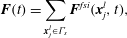


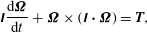







The speed of sound in this model is a constant equal to
 $c_{s}=\sqrt{1/3}$
, to preserve symmetries with the choice of equilibrium functions in (A 6) (Latt Reference Latt2007). The kinematic viscosity
 ${\it\nu}$
is related to the parameter
 ${\it\tau}$
in the last equation through
 ${\it\nu}=c_{s}^{2}({\it\tau}-0.5)$
. By keeping
 $Ma=U/c_{s}<O(0.1)$
and
 $\mathit{Kn}={\it\nu}/(c_{s}\cdot L)<O(0.1)$
(where
 $U$
and
 $L$
are the characteristic velocity and length scale, respectively), the lattice Boltzmann fluid solver is equivalent to solving the incompressible Navier–Stokes equations.
Appendix B. Determination of the equilibrium angles
${\it\phi}_{c}$
and
${\it\phi}_{us}$


The angles are found using half-interval search in the following way for a given value of
 $\mathit{Re}_{p}$
.
-
(i) Initialize at
${\it\phi}_{n}=-30^{\circ }~({\it\theta}=90^{\circ })$
. -
(ii) The particle is held steady for the first 3000 time steps, in order for the fluid to be resolved around the particle.
-
(iii) The simulation runs for 500 time steps.
-
(a) If
$\dot{{\it\phi}}<0$
and
${\it\phi}_{n}<30^{\circ }$
:-
(i) repeat from step (ii) with
${\it\phi}_{n+1}={\it\phi}_{n}+1^{\circ }$
.
-
-
(b) If
$\dot{{\it\phi}}>0$
:-
(i) find
${\it\phi}_{us}$
through a half-interval search between
${\it\phi}_{n}$
and
${\it\phi}_{n-1}$
, with the tolerance set to
${\rm\Delta}{\it\phi}=0.1^{\circ }$
; -
(ii) find
${\it\phi}_{c}$
through a half-interval search between
${\it\phi}_{n}$
and
${\it\phi}=30^{\circ }$
, with the tolerance set to
${\rm\Delta}{\it\phi}=0.1^{\circ }$
.
-
-
(c) If
${\it\phi}_{n}=30^{\circ }$
:-
(i) there are no equilibrium angles at the given
$\mathit{Re}_{p}$
(i.e.
$\mathit{Re}_{p}<\mathit{Re}_{c}$
).
-
-



Appendix C. Determination of the critical density ratio
${\it\alpha}_{c}$

The critical density ratio
 ${\it\alpha}_{c}$
is found in the following way for a given value of
 $\mathit{Re}_{p}$
.
-
(i) Initialize at
${\it\phi}_{0}={\it\phi}_{us}-{\it\delta}{\it\phi}~({\it\theta}=90^{\circ })$
with
${\it\alpha}_{n}=1$
. -
(ii) The particle is held steady for the first 3000 time steps, in order for the fluid to be resolved around the particle.
-
(iii) The particle is released and starts rotating with
$\dot{{\it\phi}}<0$
.-
(a) If the particle reaches
${\it\phi}\leqslant {\it\phi}_{0}-{\rm\pi}$
: there is no
${\it\alpha}_{c}>1$
at the given
$\mathit{Re}_{p}$
. -
(b) If the particle stops (
$\dot{{\it\phi}}\geqslant 0$
) at
${\it\phi}>{\it\phi}_{0}-{\rm\pi}$
: find
${\it\alpha}_{c}$
by a half-interval search between
${\it\alpha}=1$
and
${\it\alpha}=\mathit{St}_{max}/\mathit{Re}_{p}$
(
$\mathit{St}_{max}=600$
for the
$r_{p}=4$
spheroid), with the tolerance set to
${\rm\Delta}\mathit{St}=10$
.
-



Appendix D. Determination of
$\mathit{St}_{0.5}$

The critical Stokes number
 $\mathit{St}_{0.5}$
is found in the following way for a given value of
 $\mathit{Re}_{p}$
.
-
(i) Initialize at
${\it\phi}_{0}=-45^{\circ }~({\it\theta}=90^{\circ })$
. -
(ii) The particle is held steady for the first 500 time steps, in order for the fluid field to be resolved around the particle.
-
(iii) Set the initial angular velocity of the particle to
$\dot{{\it\phi}}=-G/2$
, where
$G$
is the shear rate of the flow. -
(iv)
$\mathit{St}_{0.5}$
is defined as the value of
$\mathit{St}$
at which
$GT=Gt_{{\it\phi}=-5{\rm\pi}}-Gt_{{\it\phi}=-3{\rm\pi}}={\rm\pi}(r_{p}^{-1}+r_{p}+2)$
, and is found by a half-interval search between
$\mathit{St}=\mathit{Re}_{p}$
(i.e.
${\it\alpha}=1$
) and
$\mathit{St}=\mathit{St}_{max}$
(
$\mathit{St}_{max}=2500$
for the
$r_{p}=4$
spheroid), with the tolerance set to
${\rm\Delta}\mathit{St}=10$
.





Appendix E. Determination of the intrinsic viscosity
${\it\eta}$

In this section we describe how to obtain the intrinsic viscosity of the one-particle suspension from the simulations in this work. The procedure is identical to that used by Huang et al. (Reference Huang, Wu and Lu2012a ,Reference Huang, Yang, Krafczyk and Lu b ). In the lattice Boltzmann scheme employed in this study, the local shear stress can be evaluated in each fluid node according to
 $$\begin{eqnarray}{\it\sigma}(\boldsymbol{x}^{e},t)=-\left(1-\frac{1}{2{\it\tau}}\right)\mathop{\sum }_{i=0}^{18}(f_{i}(\boldsymbol{x}^{e},t)-f_{i}^{eq}(\boldsymbol{x}^{e},t))c_{i,x}c_{i,y}.\end{eqnarray}$$
The total shear stress on the moving walls,
 ${\it\sigma}_{w}(t)$
, is evaluated by taking the mean value of all nodes closest to the walls (i.e. at
 $y=1$
and
 $y=N-1$
). The time-dependent intrinsic viscosity
 ${\it\eta}^{\ast }(t)$
is calculated from
 $$\begin{eqnarray}{\it\eta}^{\ast }(t)=\frac{1}{{\it\Phi}}\left(\frac{{\it\sigma}_{w}(t)}{{\it\rho}_{0}{\it\nu}G}-1\right),\end{eqnarray}$$
where
 ${\it\nu}$
and
 ${\it\rho}_{0}$
are the kinematic viscosity and density of the fluid, respectively, and
 ${\it\Phi}$
is the volume fraction calculated from
 $$\begin{eqnarray}{\it\Phi}=\left({\displaystyle \frac{4{\rm\pi}ab^{2}}{3}}\right)\bigg/N^{3},\end{eqnarray}$$
where
 $4{\rm\pi}ab^{2}/3$
is the volume of a prolate spheroid with major semi-axis
 $a$
and minor semi-axis
 $b$
and
 $N^{3}$
is the volume of the simulation domain. In order to evaluate the intrinsic viscosity for a certain rotational state at a certain
 $\mathit{Re}_{p}$
, the simulation is initialized at rest in an orientation from which the particle assumes the stable rotational state quickly, i.e.
 $({\it\phi},{\it\theta})_{1}=(0,0)$
for non-planar motion at
 $\mathit{Re}_{\mathit{LR}}<\mathit{Re}_{p}<\mathit{Re}_{T}$
,
 $({\it\phi},{\it\theta})_{2}=(5^{\circ },90^{\circ })$
for the steady state at
 $\mathit{Re}_{p}>\mathit{Re}_{c}$
and
 $({\it\phi},{\it\theta})_{3}=(-7^{\circ },90^{\circ })$
for tumbling at any
 $\mathit{Re}_{p}$
. The simulation is run up to
 $Gt=1000$
, which seemed to be enough for the value of
 ${\it\eta}^{\ast }(t)$
to converge at the walls for
 $0<\mathit{Re}_{p}<200$
. The final (time-independent) value of
 ${\it\eta}$
was evaluated through time-averaging
 ${\it\eta}^{\ast }(t)$
from
 $Gt=667$
to
 $Gt=1000$
.



