1. Introduction
A turbulent fountain is formed when there is discharge of a dense jet upward into a homogeneous, less dense environment. A similar flow occurs when a less dense fluid is injected downwards into a denser ambient fluid. At the source, the jet momentum is usually sufficient to overcome the opposing buoyancy force, and the jet rises. However, the jet slows down continually and then, after reaching its maximum penetration height, falls down as an annular plume around the inner rising jet. Prior to reaching its maximum penetration height, there is no return flow around the rising jet and the flow structure resembles that of a turbulent jet. This stage of the flow is referred to as a ‘negatively buoyant jet’ (NBJ), which is the primary focus of this study. These flows occur widely in industrial and geophysical applications, for example, heating, ventilation and air-conditioning in large buildings (Baines, Turner & Campbell Reference Baines, Turner and Campbell1990; Lin & Linden Reference Lin and Linden2005), brine discharge from desalination plants (Pincince & List Reference Pincince and List1973), explosive volcanic eruptions (Kaminski, Tait & Carazzo Reference Kaminski, Tait and Carazzo2005; Suzuki et al. Reference Suzuki, Koyaguchi, Ogawa and Hachisu2005; Carazzo, Kaminski & Tait Reference Carazzo, Kaminski and Tait2008) and the dynamics of cumulus cloud tops (Turner Reference Turner1966).
A dimensional analysis of the relevant variables in the study of an NBJ reveals two important non-dimensional parameters; the densimetric Froude number  $Fr_o = W_o/\sqrt {(g\rho ^\ast d/2)}$ and the Reynolds number
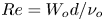 $Re = W_od/\nu _o$, with the precise value of the latter being not important with regard to mean motion in a fully turbulent jet. Here,
 $W_o$ is the source velocity,
 $d$ is the inlet diameter,
 $\nu _o$ is the kinematic viscosity of the jet fluid and
 $\rho ^{\ast } = (\rho _a-\rho _o)/\rho _a$. The subscripts ‘
 $o$’ and ‘
 $a$’ refer to the jet fluid and the ambient fluid, respectively. In the present study, we focus only on Boussinesq flows, i.e. those for which
 $|\rho _a-\rho _o|/\rho _a \leq 0.1$. In general, the evolution of the NBJ along the axis is studied via the integral quantities expressed in terms of the volume (
 $Q$), momentum (
 $M$) and buoyancy (
 $F$) fluxes, and the integral buoyancy (
 $B$) defined as
 \begin{equation} Q = 2 \int_{0}^{\infty} r W \,\textrm{d}r,\,\,\,\, M = 2 \int_{0}^{\infty} r W^2 \,\textrm{d}r,\,\,\,\, F = 2 g \rho^\ast \int_{0}^{\infty} r W C \,\textrm{d}r,\,\,\,\, B = 2 g \rho^\ast \int_{0}^{\infty} r C \,\textrm{d}r. \end{equation}
Here,  $W$,
 $C$ and
 $g \rho ^\ast C$ represent the mean axial velocity, mean concentration and mean buoyancy at a point (
 $z, r$), respectively. Note that
 $z$ and
 $r$ are the axial and radial coordinates. The integral quantities are then used to define the characteristic velocity (
 $W_m$), width (
 $r_m$) and buoyancy (
 $b_m$) for the NBJ as
 \begin{equation} W_m = \frac{M}{Q},\quad r_m = \frac{Q}{M^{1/2}},\quad b_m = \frac{BM}{Q^2}, \end{equation}
which lead to the definitions of local Froude number ( $Fr_z$) and local Richardson number (
 $Ri_z$) at a given axial location as
 \begin{equation} Fr_z = \frac{W_m}{(r_m b_m)^{1/2}} = \frac{1}{Ri_z^{1/2}}. \end{equation}
The majority of experimental studies in the past have studied the bulk flow behaviour of turbulent fountains using flow visualisation techniques. For example, Turner (Reference Turner1966), Baines et al. (Reference Baines, Turner and Campbell1990), Bloomfield & Kerr (Reference Bloomfield and Kerr1998), Zhang & Baddour (Reference Zhang and Baddour1998) and Williamson et al. (Reference Williamson, Srinarayana, Armfield, McBain and Lin2008) made measurements of fountain rise heights which encompass very weak, weak and forced fountains. Later, Burridge & Hunt (Reference Burridge and Hunt2012, Reference Burridge and Hunt2013) conducted experiments over a wide range of Froude number spanning very weak to highly forced fountains. The motivation behind all these studies was to obtain scaling relationships for rise height, the time scale of fluctuations in the rise height in terms of  $Fr_o$, and develop integral models for describing the mean behaviour of a turbulent fountain.
Other experimental studies utilised different measurement techniques to obtain detailed measurements of velocity and temperature in an NBJ. For instance, Mizushina et al. (Reference Mizushina, Ogino, Takeuchi and Ikawa1982) used hot-wire and cold-wire anemometry to measure velocity and temperature fluctuations in a high- $Fr_o$-number fountain. They found that the mean velocity and temperature profiles were similar to a neutral jet (NJ) but wider. Cresswell & Szczepura (Reference Cresswell and Szczepura1993) used laser Doppler anemometry and fast response thermocouples to simultaneously measure velocity and temperature fluctuations in an NBJ. They analysed the energy budget equations and reported that the contribution of negative buoyancy was limited to the mean motion, with very little influence on the turbulence. Cresswell & Szczepura (Reference Cresswell and Szczepura1993) also showed that the widening of NBJ was due to turbulent entrainment near the source, after which it was due to deceleration of the jet by buoyancy forces.
From a theoretical approach, models have been proposed to predict the rise height and entrainment in the NBJ (Papanicolaou, Papakonstantis & Christodoulou Reference Papanicolaou, Papakonstantis and Christodoulou2008) and weak to highly forced fountains (McDougall Reference McDougall1981; Bloomfield & Kerr Reference Bloomfield and Kerr1998; Kaye & Hunt Reference Kaye and Hunt2006). The basis of these models is the pioneering work on positively buoyant jets/plumes by Morton, Taylor & Turner (Reference Morton, Taylor and Turner1956), which has been later developed for modelling the initial rise of the NBJ (Abraham Reference Abraham1967; Bloomfield & Kerr Reference Bloomfield and Kerr2000; Papanicolaou & Kokkalis Reference Papanicolaou and Kokkalis2008). The two aspects that are critical in the theoretical modelling of a negatively buoyant jet in this manner are (i) the entrainment coefficient and (ii) the validity of self-similarity. For instance, Milton-McGurk et al. (Reference Milton-McGurk, Williamson, Armfield and Kirkpatrick2020a) and Kaminski et al. (Reference Kaminski, Tait and Carazzo2005) found evidence that entrainment is significantly lower in an NBJ compared with a NJ or positively buoyant jet. Likewise, Papanicolaou et al. (Reference Papanicolaou, Papakonstantis and Christodoulou2008) found that a reduced entrainment coefficient is mandatory for the models to accurately predict the rise height of a turbulent fountain.
Using numerical simulations, Williamson, Armfield & Lin (Reference Williamson, Armfield and Lin2011) investigated fountains in the range  $4 \leq Fr_o \leq 7$ and observed that in an established fountain flow, apart from a short developing region near the source, the entrainment coefficient is lower than in the NJ. It has also been reported via experimental studies that the entrainment coefficient varied with local Froude number for jets with momentum and initial buoyancy (Kaminski et al. Reference Kaminski, Tait and Carazzo2005). In addition, Mizushina et al. (Reference Mizushina, Ogino, Takeuchi and Ikawa1982) and Williamson et al. (Reference Williamson, Armfield and Lin2011) observed that both the inner and the outer flows in a turbulent fountain continuously developed so the flow never attains self-similarity and the flow statistics vary with
 $z$ and
 $Fr_z$.
In a companion paper (Milton-McGurk et al. Reference Milton-McGurk, Williamson, Armfield, Kirkpatrick and Talluru2020b), we studied the development of mean velocity and buoyancy profiles for a range of  $Fr_z$ along the axis of the NBJ. It was observed that the NJ and the NBJ are similar in the forced regime,
 $Fr_z \gtrsim 3.0$. Interestingly, even outside the forced regime, the velocity and buoyancy profiles in the NBJ exhibit self-similar Gaussian shapes over a wide range of
 $Fr_z$ when scaled with the local centreline values (
 $W_c,C_c$) and the respective jet half-widths (
 $r^\ast _{W},r^\ast _{C}$), just as in the NJ. Note that
 $r^\ast _{W}$ and
 $r^\ast _{C}$ represent the radial distance from the axis, where the mean axial velocity (
 $W$) and concentration (
 $C$) are equal to half of the corresponding centreline values, i.e.
 $W(r^\ast _{W})/W_c = 0.5$ and
 $C(r^\ast _{C})/C_c = 0.5$. However, the turbulence intensity and Reynolds stress profiles do not scale with
 $W_c^2$ due to the strongly decelerating mean flow, particularly at lower
 $Fr_z$. A new velocity scale defined based on turbulent momentum flux was found to collapse the turbulence intensities onto a single curve. Further, we noticed that the entrainment is generally lower in the NBJ than the NJ even in the forced regime near the source consistent with previous studies (Kaminski et al. Reference Kaminski, Tait and Carazzo2005; Papanicolaou et al. Reference Papanicolaou, Papakonstantis and Christodoulou2008; Milton-McGurk et al. Reference Milton-McGurk, Williamson, Armfield and Kirkpatrick2020a).
Summing up the above findings, the development of the NBJ can be described as follows. Closer to the source, the NBJ behaves similar to a momentum-driven jet, where the production of turbulence stresses is governed by the radial velocity gradient. Hence, both the mean flow and turbulence intensities scale well with the centreline velocity as observed in the NJ. As the NBJ develops (i.e. as the local Froude number decreases), the mean flow continues to exhibit self-similar Gaussian form when scaled with the local velocity and length scales,  $W_c$ and
 $r^\ast _{W}$, although the NBJ grows more rapidly than the NJ. In contrast, the turbulence stresses do not scale with
 $W^2_c$; they increase continuously relative to
 $W_c^2$ due to strongly decelerating mean flow in the NBJ. This suggests that the link between the mean velocity gradient and turbulence production in the NBJ is not the same as in the NJ. Thus, it is possible to postulate that the NBJ transitions from a momentum-driven jet with strong local turbulence production, to a jet with decelerating mean and decaying turbulence as
 $Fr_z$, decreases from
 $Fr_o$ to 0.
Based on the analysis of total kinetic energy (known as TKE) equation for a low Froude number turbulent fountain, Cresswell & Szczepura (Reference Cresswell and Szczepura1993) showed that the local total kinetic energy production is predominantly governed by mean flow gradients and turbulent diffusion throughout most of the flow up to the cap region. But, Milton-McGurk et al. (Reference Milton-McGurk, Williamson, Armfield, Kirkpatrick and Talluru2020b) showed that in the NBJ, the Reynolds stresses decay at a different rate compared with the mean flow as a result of negative buoyancy. Hence, it is not well-understood as to how the internal structure of the NBJ is affected by buoyancy. In our previous work (Milton-McGurk et al. Reference Milton-McGurk, Williamson, Armfield, Kirkpatrick and Talluru2020b), we identified how the mean flow statistics develop and obtained separate velocity scales for mean velocity and turbulence intensity profiles. In this paper, we will specifically investigate the turbulence structure in the NJ and the NBJ to assess how the local conditions affect correlation length scales, spectra and probability density functions (p.d.f.s).
The paper is organised as follows. In § 2, we describe the experimental set-up used in this study for obtaining velocity and concentration measurements in the NJ and the NBJ. A comparison of the mean and turbulence structure in these flows is made in § 3. This is followed by a discussion on velocity-concentration correlations, spectra and p.d.f.s in § 4, § 5, § 6 and § 7. A summary of the key conclusions is given in § 8.
2. Experimental details
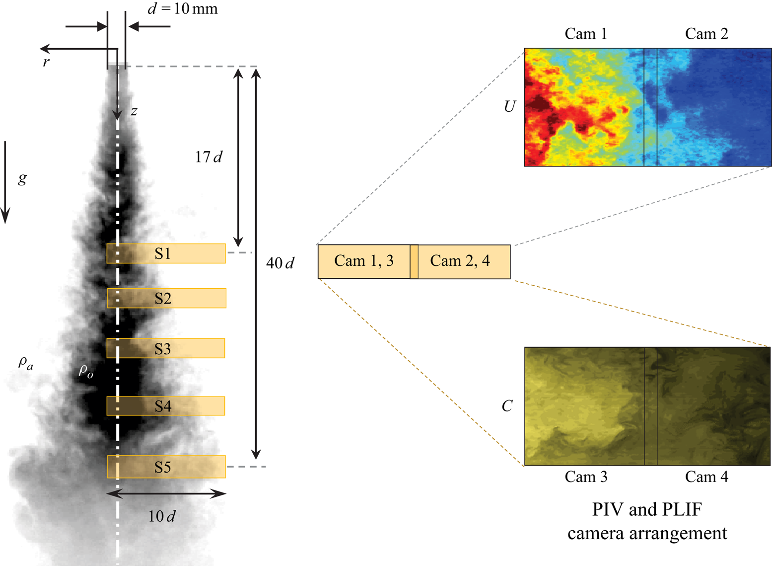
Experiments are carried out in a glass-walled water tank, whose dimensions are  $1\ \textrm {m} \ (\text {length}) \times 1\ \textrm {m}\ (\textrm {width}) \times 1\ \textrm {m}\ (\textrm {height})$. Two sets of experiments are performed by varying the ambient and the source fluids. The NJ is obtained when fresh water is used as both the ambient and the source fluid. In the NBJ experiments, fresh water is used as the source fluid and salt water as the ambient as shown in figure 1. In all the experiments, the jet is injected downwards into the water tank and its flow rate is set using ISMATEC MCP-Z series gear pump with an accuracy of 1 %. The source fluid is drawn from a separate container outside the main water tank. In a typical experiment, the amount of source fluid added to the 800 litres of ambient fluid in the main tank is less than 4 litres. This results in an increase of less than 0.5 % in the water level, which we believe has negligible effect on the development of the jet.
A snapshot taken during the NBJ experiment. Fresh water at density ( $\rho _o$) is injected into the ambient salt water of density (
 $\rho _a$). The coloured regions indicate the five measurement locations S1 to S5. The inset shows the arrangement of four cameras (cam 1 and cam 2 – PIV; cam 3 and cam 4 – LIF), the velocity and the concentration fields. Note that cam 1, cam 3 and cam 2, cam 4 have the same field of view. Dimensions not to scale.

The salinity of the ambient fluid, the inlet flow rate and the pipe diameter ( $d$) are varied to obtain the desired Reynolds and Froude numbers for the NBJ. In order to have proper comparison between the NJ and the NBJ, the inlet parameters of the jet are chosen such that the source Reynolds number is the same in both of these experiments. The ratio of pipe length and pipe diameter is greater than 80 (Patel Reference Patel1974) to ensure that the flow is fully developed as it enters the water tank. It is well known that the salinity affects the viscosity of the ambient fluid, and in this study it has a value of
 $1.01\times 10^{-6}\ \textrm {m}^2\ \textrm {s}^{-1}$ for
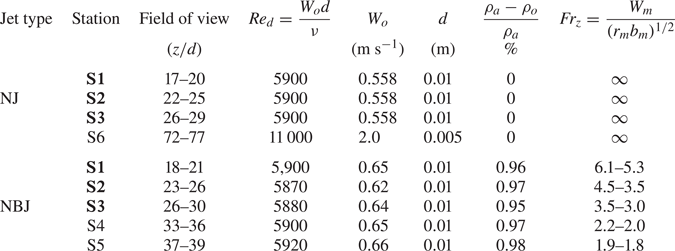
 $(\rho _a-\rho _o)/\rho _a = 0.01$. Thus, the ratio of the viscosity of ambient fluid and the source fluid is approximately 0.92. Experiments at six different locations between 17 and 77 diameters downstream are conducted, which are marked as S1 to S6. Out of these, stations S1, S2 and S3 are common to the NJ and the NBJ experiments.
Typically, a fully turbulent jet is achieved at  $Re > 10\,000$ and it exhibits self-similar behaviour beyond
 $z/d = 50$ (Panchapakesan & Lumley Reference Panchapakesan and Lumley1993). Hence, we carried out an NJ experiment at
 $Re = 11\,000$ at measurement station S6 (
 $z/d = 77$) and the results were compared against those in the literature. As will be discussed later, there is a very good agreement between the present study and that of PL1993 (Panchapakesan & Lumley Reference Panchapakesan and Lumley1993) at the same
 $Re$, which validates the measurement set-up used in this study. Further, our present study is directly comparable to Wang & Law (Reference Wang and Law2002), who studied turbulent NJ experimentally at
 $Re = 6000$ with water as the fluid medium. In the NBJ experiments, we were limited to
 $Re = 5900$ due to the constraints of ambient and source fluids, size of the tank and the camera/laser set-up. Since the focus of this study is the direct comparison between the NJ and the NBJ,
 $Re$ is maintained to be the same (i.e. 5900) in all the experiments to avoid any Reynolds number effects. The experimental parameters at these measurement stations are summarised in table 1.
Experimental parameters used in the study of NJ and NBJ. Measurement stations S1, S2 and S3 (in bold fonts) are common to NJ and NBJ experiments, while station S6 represents a self-similar turbulent NJ.

A combination of particle image velocimetry (PIV) and planar laser induced fluorescence (LIF) measurement techniques is used to obtain simultaneous velocity and concentration (equivalent to density) measurements in the axial plane of the jet. Full details of the experimental procedures that account for non-uniform laser profile, variations in the laser power with time, mismatch of refractive index in the ambient and the source fluids have been comprehensively discussed in Milton-McGurk et al. (Reference Milton-McGurk, Williamson, Armfield and Kirkpatrick2020a), and therefore will only be briefly discussed here. A dual-pulsed Nd-YAG laser ( $200\ \textrm {mJ}\ \textrm {pulse}^{-1}$ at 532 nm) is used to provide illumination for PIV experiments with a pulse separation of 0.25 ms. Naturally occurring particles of size in the range of
 $0.1\text {--}10\ \mathrm {\mu }\textrm {m}$ in tap water (with Stokes number
 $\ll 1$), are used as tracers for PIV.
For the LIF measurements, a fluorescent dye Rhodamine 6G is chosen as the scalar tracer, which has a peak emission at 560 nm. Images are captured using four pco.2000 cameras (two each for PIV and LIF measurements) with a pixel resolution of  $2048 \times 2048$ at a rate of 7 Hz. The PIV cameras are fitted with a
 $532 \pm 2\ \textrm {nm}$ bandpass filter to filter out ambient light and the Rhodamine 6G dye fluorescence. A
 $\textrm {B}+\textrm {W}$ Orange MRC 040M filter was used on the LIF cameras to cut off light below approximately 550 nm, allowing only the fluorescence from the dye, but not the scattered light from the particles, through to the CCD sensor.
A snapshot of the instantaneous PIV and LIF images taken in one of the NBJ experiments is shown in figure 1, which also highlights the experimental parameters ( $\rho _o, \rho _a$), the field of view and the measurement locations used in the study. The inset plot shows the arrangement of two cameras for PIV (cam 1 and cam 2) and two cameras for LIF (cam 3 and cam 4) with a small overlap between the images. Using the calibration image that is common to all the cameras, the images are stitched during the post-processing stage to yield a larger field of view. The final processed velocity and concentration fields are shown on the right-hand side of figure 1. In our initial campaign of experiments, it was found that the jet is well-behaved and is symmetric about its axis. Hence, the experiments were performed only on one side of the jet axis (as shown in figure 1) to allow for larger
 $Fr_o$ (or larger range of scales) to be achieved while maintaining high spatial resolution.
For a turbulent fountain with high-source Reynolds ( $Re > 2000$) and Froude numbers (
 $Fr_o \gtrsim 4$), the steady state height (
 $z_{ss}$) and the initial rise height (
 $z_i$) of the NBJ have been shown to scale with
 $Fr_o$ as
 ${z_{ss}}/{r_o} = 2.46\,Fr_o$, with
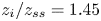 ${z_i}/{z_{ss}} = 1.45$ (Turner Reference Turner1966; Burridge & Hunt Reference Burridge and Hunt2012, Reference Burridge and Hunt2014). In the present NBJ experiments at
 $Fr_o = 30$, the initial rise height of the NBJ is
 $z_i/d \sim 54$, and the steady rise height
 $z_{ss}/d \sim 37$ and this study reports measurements for up to
 $z/d = 39$. Throughout this paper,
 $r$ and
 $z$ will be used to represent the radial and axial directions, respectively, while
 $\tilde {U}$ and
 $\tilde {W}$ represent the corresponding instantaneous velocity components. Further,
 $\tilde {W} = W + w$ and
 $\tilde {C} = C+c$, where the upper case and the lower case letters represent the time-averaged mean and fluctuating quantities, respectively.
Each experiment consisted of several runs, and each run lasted for 45 s during which images were captured at seven frames per second. The volumetric flow rate was computed from each realisation, which was then used for identifying the ‘NJ’ and the ‘NBJ’ phases of the flow (see Milton-McGurk et al. (Reference Milton-McGurk, Williamson, Armfield and Kirkpatrick2020a,Reference Milton-McGurk, Williamson, Armfield, Kirkpatrick and Tallurub) for a full description). In the NJ experiments, it was observed that the flow reached the steady state within the first five seconds from the start and remained steady thereafter. In the NBJ, the flow experiences continuous deceleration due to opposing buoyancy and comes to rest momentarily before the flow returns. For this reason, several runs were conducted in the NBJ in comparison with the NJ experiments to get the required number of realisations for statistical convergence.
In a typical NBJ experiment, the steady state phase of the NBJ was observed between 5 and 20 s from the start before the flow returned (see Milton-McGurk et al. (Reference Milton-McGurk, Williamson, Armfield, Kirkpatrick and Talluru2020b) for full details). Further, as one would expect, the time duration available for acquiring meaningful data (i.e. uncontaminated by the return flow) decreased with distance away from the source. For instance, at station S5, a time interval of 5–6 s was available for the NBJ phase. Therefore, we varied the number of runs between six and 20 at different stations to obtain a minimum of 800 images at each measurement location. Once the steady state phase of the flow was identified, the images during that stage were ensemble averaged to obtain the mean velocity and concentration fields, and the fluctuating components were then estimated by subtracting each of the individual realisations from the mean fields. The advantage of the ensemble mean is that the spatial variation of mean velocity and concentration is properly accounted for when computing the instantaneous fluctuating velocity and concentration fields.
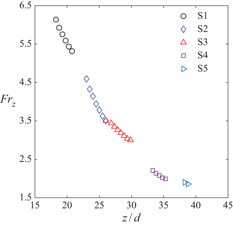
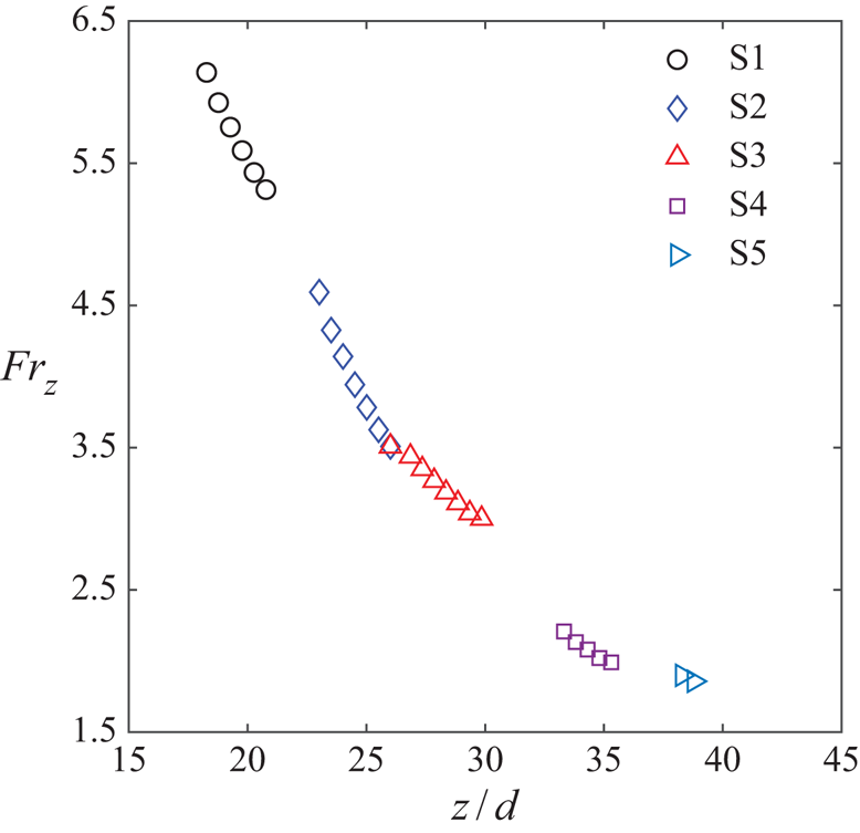
Using the mean velocity and concentration profiles, we estimated the local Froude number ( $Fr_z$) as per (1.1a–d)–(1.3), and the results of
 $Fr_z$ at different axial locations are plotted in figure 2. It is clear that
 $Fr_z$ decreases quite rapidly along the axis, for instance,
 $Fr_z$ decreased from a value of 30 at the source to 6.1 within a short distance of
 $z/d = 18$ from the jet outlet. Most importantly,
 $Fr_z$ is less than 4.5 at stations S2 and beyond, which indicates that the NBJ is not momentum driven at these locations and there is strong opposing force due to buoyancy at these locations.
Variation of  $Fr_z$ along the axis of the NBJ at source Froude number,
 $Fr_o = 30$.
3. Mean and turbulence statistics
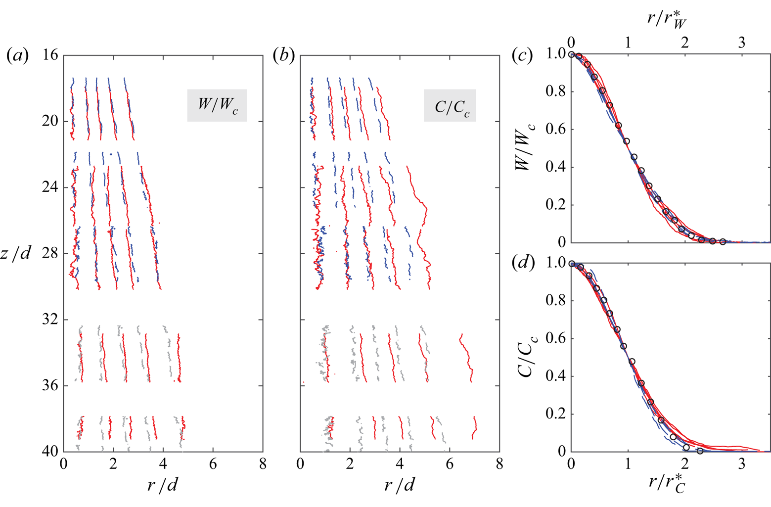
In this section, we will present the general characteristics of the mean flow in the NBJ in comparison with the NJ. Figures 3(a) and 3(b) shows the contour maps of mean axial velocity ( $W/W_c$) and concentration (
 $C/C_c$) at five different measurement locations (see figure 1 and table 1). The contours
 $W/W_c$ and
 $C/C_c$ are plotted as a function of radial (
 $r/d$) and axial (
 $z/d$) coordinates along abscissa and ordinate axes, respectively. The consistent trends observed in
 $W/W_c$ and
 $C/C_c$ at five axial locations (measurements taken on different days) clearly validate the experimental procedures employed in this study.
Contours of normalised (a) velocity ( $W/W_c$) and (b) concentration (
 $C/C_c$) plotted as a function of
 $r/d$ and
 $z/d$. Here,
 $W_c$ and
 $C_c$ are the centreline velocity and concentration. The contours are drawn at levels 0.15 to 0.95 in steps of 0.2. Normalised mean (c) velocity and (d) concentration profiles in the radial direction plotted as a function of
 $r/r^\ast _W$ and
 $r/r^\ast _C$, where
 $r^\ast _W$ and
 $r^\ast _C$ are the corresponding half-widths (Milton-McGurk et al. Reference Milton-McGurk, Williamson, Armfield, Kirkpatrick and Talluru2020b). Black circles in panels (c,d) are the self-similar mean velocity and concentration profiles taken from Panchapakesan & Lumley (Reference Panchapakesan and Lumley1993) and Dowling & Dimotakis (Reference Dowling and Dimotakis1990), respectively. Blue dashed and red solid contour lines represent the NJ and the NBJ, respectively. The grey dashed lines in panels (a,b) are the interpolated results at S4 and S5 obtained via linear interpolation of NJ data at stations S1, S2, S3 and S6.

Looking at the results in figures 3(a) and 3(b), we find that the width of the mean scalar field in both the NJ and the NBJ is larger than the axial velocity field. The greater radial spread of scalar field in the NJ can be explained using a simple approach given by Morton (Reference Morton1959). In contrast, the radial spread of scalar in the NBJ is not easy to model using simple integral equations. In our previous study (Milton-McGurk et al. Reference Milton-McGurk, Williamson, Armfield, Kirkpatrick and Talluru2020b), we found that both the ratio ( $\lambda$) of scalar and velocity profile widths and the entrainment coefficient in the NBJ are second-order functions of
 $Fr_z^{-1}$, equivalently, they are linear functions of
 $Ri_z$. While
 $\lambda$ is found to remain relatively constant in the NJ,
 $\lambda$ increases nonlinearly along the axis of the NBJ. It is quite clear that the NBJ is spreading faster than the NJ, which has been previously reported to be the consequence of deceleration of the mean flow by negative buoyancy (Milton-McGurk et al. Reference Milton-McGurk, Williamson, Armfield and Kirkpatrick2020a,b).
Figures 3(c) and 3(d) shows the mean velocity and concentration profiles in the NJ and the NBJ, where the radial coordinate is normalised by the respective jet half-widths. The data for the NJ (black symbols) taken from Panchapakesan & Lumley (Reference Panchapakesan and Lumley1993) are also included in figure 3(c), for comparison. Overall, there is excellent agreement with the results of Panchapakesan & Lumley (Reference Panchapakesan and Lumley1993). Further, it is clear that all the profiles in the NJ and the NBJ collapse well onto a single curve that resembles a Gaussian curve of the form
 \begin{equation} \frac{W}{W_c} = \exp\left[-{\ln(2)}\left(\frac{r}{r^\ast_{W}}\right)^2\right];\quad \frac{C}{C_c} = \exp\left[-{\ln(2)}\left(\frac{r}{r^\ast_{C}}\right)^2\right]. \end{equation}
Note that ln(2) is used in the above Gaussian expressions to be consistent with the definitions of jet half-widths,  $r^\ast _{W}$ and
 $r^\ast _{C}$.
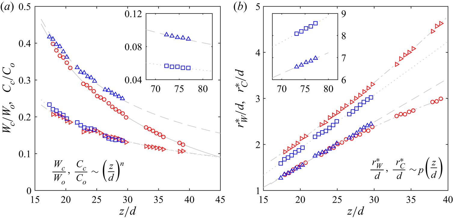
The variation of  $W_c$,
 $C_c$,
 $r^\ast _{W}$ and
 $r^\ast _{C}$ along
 $z$ are plotted in figure 4(a,b). As expected,
 $W_c$ and
 $C_c$ in the NJ decay as
 $z^{-1}$ and agree well with the results of Westerweel et al. (Reference Westerweel, Fukushima, Pedersen and Hunt2009) (see table 2). Further,
 $r^\ast _{W}$ and
 $r^\ast _{C}$ in the NJ increase linearly with
 $z$. In the NBJ, neither
 $W_c$ or
 $C_c$ exhibit simple power-law behaviour and nor do
 $r^\ast _{W}$ and
 $r^\ast _{C}$ vary in a linear fashion. A closer observation of results in the NBJ suggests that the departure from the NJ starts at
 $z/d \approx 25$, where
 $r^\ast _{W}$ and
 $r^\ast _{C}$ deviate from the linear curves. The local Froude number at this location is
 $Fr_z = 4$. According to the classification of fountains given in Hunt & Burridge (Reference Hunt and Burridge2015),
 $Fr_z = 4$ represents the upper limit of intermediate fountains. As
 $Fr_z$ continues to decrease with
 $z$, buoyancy becomes the predominant force and the flow behaves similarly to a weak and a very weak fountain. Overall, the results presented in figure 4 suggest that the mean flow is affected by negative buoyancy resulting in a faster decay of the centreline velocity
 $W_c$ and a nonlinear growth of
 $r^\ast _{W}$ and
 $r^\ast _{C}$ in the NBJ. Experimentally, we observed that the NBJ develops differently from the NJ in several aspects: (i) both the flows decelerate but the NBJ decelerates more rapidly (Milton-McGurk et al. Reference Milton-McGurk, Williamson, Armfield and Kirkpatrick2020a,b), (ii) the turbulent Schmidt number (the ratio between eddy viscosity and eddy diffusivity) is not constant and (iii) entrainment has local
 $Fr_z$ dependence (Milton-McGurk et al. Reference Milton-McGurk, Williamson, Armfield, Kirkpatrick and Talluru2020b). The integral models based on the work of Morton et al. (Reference Morton, Taylor and Turner1956), Priestley & Ball (Reference Priestley and Ball1955) and van Reeuwijk & Craske (Reference van Reeuwijk and Craske2015) can be successfully applied to explain these differences, taking into account the above items (i)–(iii), and we refer the reader to the companion paper, Milton-McGurk et al. (Reference Milton-McGurk, Williamson, Armfield, Kirkpatrick and Talluru2020b), for a comprehensive discussion.
(a) The centreline mean velocity and concentration and (b) the half-widths  $r^\ast _{W}$ and
 $r^\ast _{C}$ for the velocity field and the scalar field as a function of distance from the nozzle. Symbols:
 $\circ$, red, NBJ (
 $W_c, r^\ast _{W}$);
 $\triangleright$, red, NBJ (
 $C_c, r^\ast _{C}$);
 $\triangle$, blue NJ (
 $W_c, r^\ast _{W}$);
 $\square$, blue NJ (
 $C_c, r^\ast _{C}$). The inset figures show the results for NJ at
 $z/d = 75$. The grey lines are the empirical curve fits to the experimental data.

Comparison of the decay exponent ( $n$) for the mean velocity
 ${W_c}/{W_o}$ and mean concentration
 ${C_c}/{C_o}$ along the jet axis, and the slope (
 $p$) in the linear growth of
 $r^\ast _{W}/d$ and
 $r^\ast _{C}/d$ in the NJ. The bottom row indicates the values reported in Westerweel et al. (Reference Westerweel, Fukushima, Pedersen and Hunt2009). (The abbreviation PLIF stands for planar LIF).

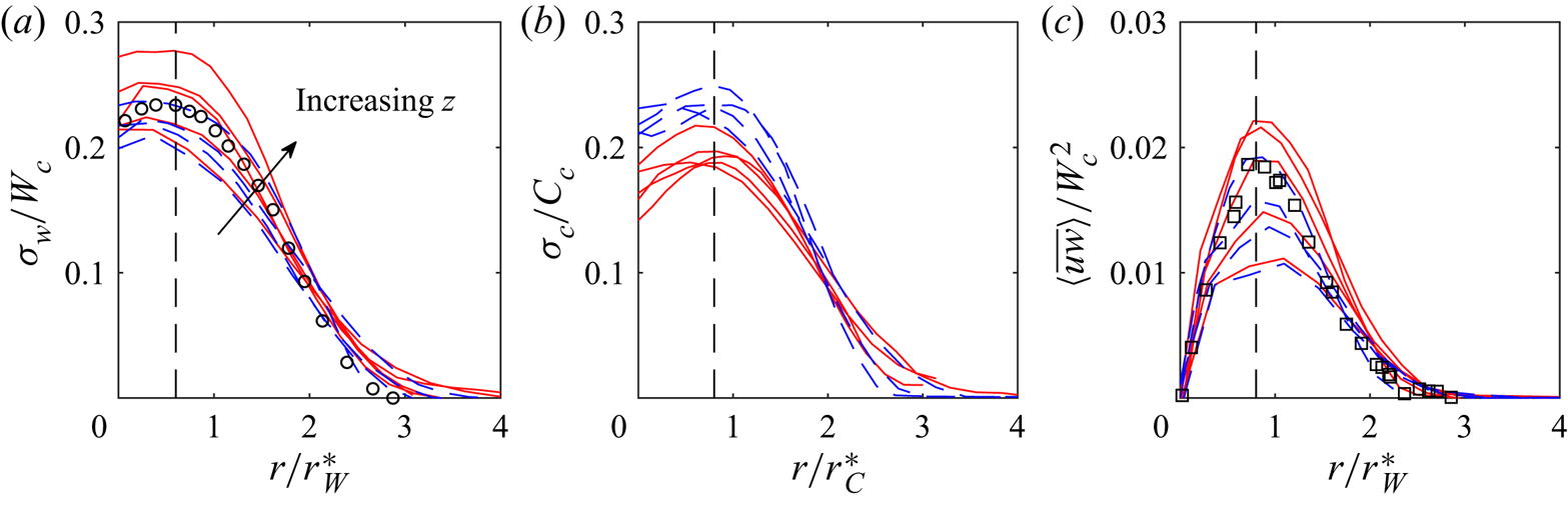
Figures 5(a) and 5(b) compares the statistics of  $\sigma _w/W_c$ and
 $\sigma _c/C_c$ in the NJ and the NBJ. Here,
 $\sigma _w = \sqrt {\langle \overline {w^2}\rangle }$,
 $\sigma _c = \sqrt {\langle \overline {c^2}\rangle }$ and the symbol ‘
 $\langle ^{\overline {~~}}\rangle$’ represents averaging over time and space (across a width of one diameter along
 $z$). The values of
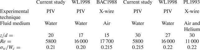
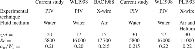
 $\sigma _w$ on the jet axis in the current study agree well with those reported for a NJ, see table 3. Further, there is a clear off-axis peak in
 $\sigma _w$ and
 $\sigma _c$ occurring at
 $r/r^\ast _{W} \approx 0.6$ and
 $r/r^\ast _{C} = 0.8$ as noted in previous studies (Wygnanski & Fiedler Reference Wygnanski and Fiedler1969; Panchapakesan & Lumley Reference Panchapakesan and Lumley1993; Weisgraber & Liepmann Reference Weisgraber and Liepmann1998; Westerweel et al. Reference Westerweel, Fukushima, Pedersen and Hunt2009). The profiles of
 $\sigma _w$ and
 $\sigma _c$ in the NJ approach a self-similar profile, which is complete at
 $z/d = 77$. On the other hand,
 $\sigma _w/W_c$ in the NBJ continuously changes with
 $z$, implying that turbulence fluctuations do not scale with
 $W_c$. Although the magnitude of
 $\sigma _c/C_c$ in the NBJ is found to be smaller than those in the NJ, a clear monotonic trend in
 $z$ is not observed in the profiles of
 $\sigma _c/C_c$ in the NBJ. On the positive side, we notice that
 $\sigma _w/W_c$ and
 $\sigma _c/C_c$ in both the NJ and the NBJ scale well with the local jet half-widths,
 $r^\ast _{W}$ and
 $r^\ast _{C}$.
Comparison of normalised root mean square value of (a) velocity,  $\sigma _w/W_c$ and (b) concentration fluctuations,
 $\sigma _c/C_c$ measured in the NJ (blue dashed lines) and the NBJ (red solid lines). (c) Reynolds stress (
 $\langle \overline {uw}\rangle /W_c^2$) profiles at
 $z/d = 18$, 23, 28, 76 in the NJ and
 $z/d = 19$, 24, 28, 35, 38 in the NBJ. The arrow indicates the trend of measurements taken at increasing
 $z$. Black circles in panel (a) and squares in panel (c) are the NJ data taken from Westerweel et al. (Reference Westerweel, Fukushima, Pedersen and Hunt2009) at
 $z/d = 80$. The vertical dashed lines indicate the off-axis peaks.

Comparison of turbulence intensities ( $\sigma _w/W_c$) on the centreline of a NJ against previous studies – PL1993 (Panchapakesan & Lumley Reference Panchapakesan and Lumley1993), BAC1998 (Browne, Antonia & Chua Reference Browne, Antonia and Chua1988) and WL1998 (Weisgraber & Liepmann Reference Weisgraber and Liepmann1998).
The radial distributions of Reynolds stress ( $\langle \overline {uw}\rangle /W_c^2$) are shown in figure 5(c). Similar to
 $\sigma _w/W_c$ and
 $\sigma _c/C_c$, there is an off-axis peak in
 $\langle \overline {uw}\rangle /W_c^2$ at
 $r/r^\ast _{W} \approx 0.8$. This off-axis peak in
 $\langle \overline {uw}\rangle$ is expected as the distribution of shear production of kinetic energy has a distinct off-axis peak at approximately the same location. In the case of NJ, we observe that
 $\langle \overline {uw}\rangle /W_c^2$ does not scale with
 $W_c$ near the source but becomes self-similar beyond
 $z/d = 50$ (see Milton-McGurk et al. (Reference Milton-McGurk, Williamson, Armfield, Kirkpatrick and Talluru2020b), for example). On the other hand,
 $\langle \overline {uw}\rangle /W_c^2$ in the NBJ does not scale with
 $W_c$ at all measurement locations, but the radial coordinate scales well with jet half-width. Overall, the analysis of
 $\sigma _w$ and
 $\langle \overline {uw}\rangle$ shows that the mean flow and the turbulence have different development characteristics in the NBJ.
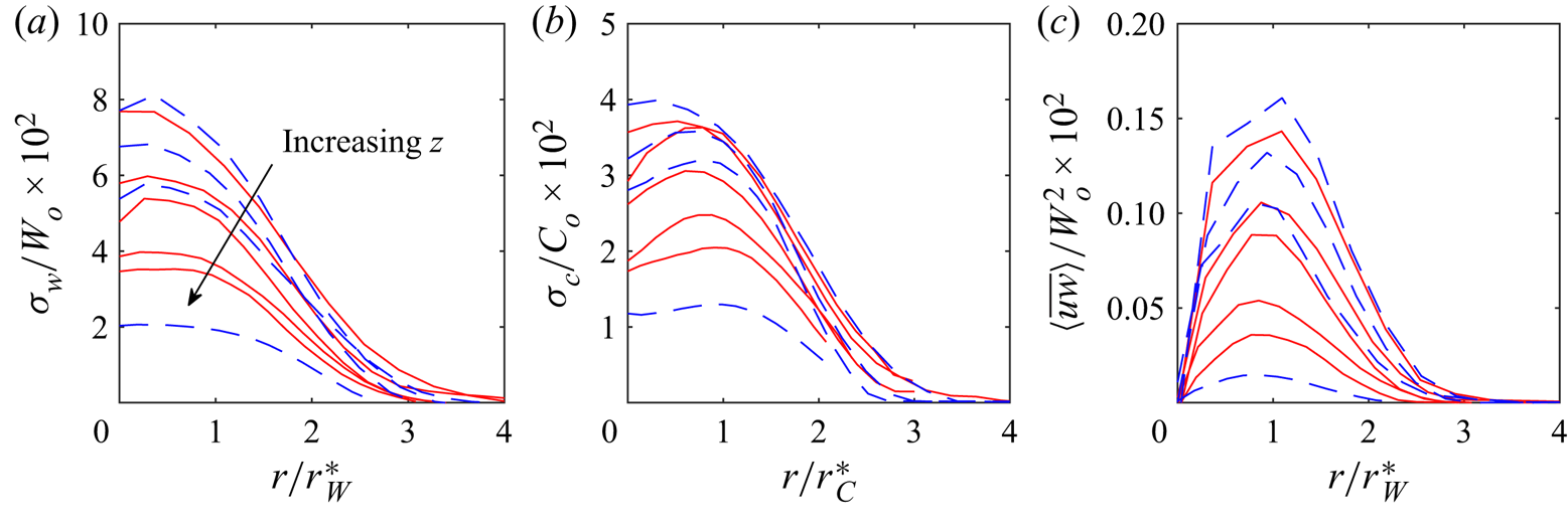
Looking further, the statistics of turbulence intensity and Reynolds stress in the NJ and the NBJ are plotted in figure 6(a)–(c) by normalising with the source velocity ( $W_o$) and concentration (
 $C_o$) for a proper comparison between the two flows. We note that the magnitudes of turbulence intensities and Reynolds stress are similar in both the flows, and they decrease with
 $z$. This suggests that the trends of
 $\sigma _w/W_c$ and
 $\langle \overline {uw}\rangle /W_c^2$ observed in figure 5 are merely due to differences in the decay of
 $W_c$ in the NJ and the NBJ. Based on the results in figures 4 and 5, it is clear that the turbulence statistics (when scaled with source conditions,
 $W_o$ and
 $C_o$) are almost similar between the NJ and the NBJ. Further, the apparent differences between the NJ and the NBJ observed in figure 4 are due to using local centreline velocity and concentration as the scaling parameters. Overall, the results indicate that negative buoyancy only affects the mean flow and not the turbulence quantities in the NBJ.
Data in figure 5(a)–(c) are plotted here using source velocity ( $W_o$) and concentration (
 $C_o$) for normalising the turbulence intensity and Reynolds stress profiles.

4. Spatial correlations and integral length scales
In order to understand the evolution of turbulent fluctuations, we need to know how  $w$ and
 $c$ are correlated over different spatial distances. This is typically studied by computing the autocorrelation functions in the axial and radial directions, which are, respectively, defined as
 \begin{equation} R^{{{z}}}_{ii}(\hat{z}, \hat{r}) = \frac{\overline{i(\hat{z}, \hat{r})i(\hat{z}+{z^\prime}, \hat{r})}}{\sigma^2_i(\hat{z}, \hat{r})}; \quad R^{{{r}}}_{ii}(\hat{z}, \hat{r}) = \frac{\overline{i(z, \hat{r}) i(z, {\hat{r} + {r}})}}{\sigma^2_i(\hat{z}, \hat{r})}; \quad i = w,u,c. \end{equation}
Note that the superscripts  ${z}$ and
 ${r}$ in
 $R^{{{z}}}_{ii}(\hat {z}, \hat {r})$ and
 $R^{{{r}}}_{ii}(\hat {z}, \hat {r})$ indicate the direction of correlation. The variance of a physical quantity
 $i$ at a point
 $(\hat {z}, \hat {r})$ in the flow is represented as
 ${\sigma ^2_i(\hat {z}, \hat {r})}$. Further,
 $\hat {z} = 0$ and
 $\hat {r} = 0$ represent the corresponding zero-shift spatial correlations, which leads to
 $R^{{{z}}}_{ii}(\hat {z} = 0,\hat {r}) = 1$ and
 $R^{{{r}}}_{ii}(\hat {z}, \hat {r} = 0) = 1$. Note that
 $R^{{{z}}}_{ii}(\hat {z}, \hat {r})$ and
 $R^{{{r}}}_{ii}(\hat {z}, \hat {r})$ are equivalent to the longitudinal and lateral correlation functions defined in Wygnanski & Fiedler (Reference Wygnanski and Fiedler1969).
4.1. Along the axis,  $R^{{{z}}}_{ii}$

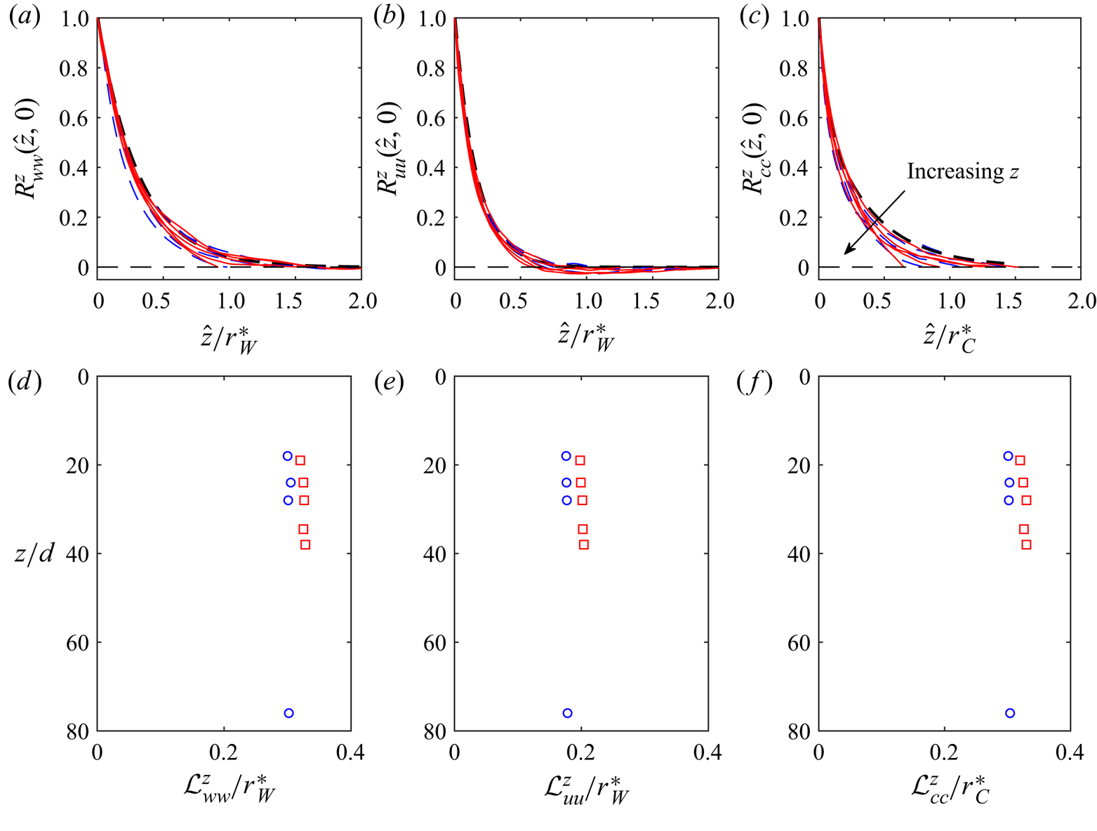
Figure 7(a)–(c) shows the autocorrelation functions  $R^{{{z}}}_{ww}$,
 $R^{{{z}}}_{uu}$ and
 $R^{{{z}}}_{cc}$ on the jet centreline (
 $\hat {z}$, 0) plotted as a function of normalised separation distance,
 $\hat {z}/r^\ast _{W}$. Note that only the data for positive
 $\hat {z}$ are shown here. In each subplot, the results at four locations (
 $z/d = 18$, 23, 28 and 76) in the NJ and five locations (
 $z/d = 19$, 24, 28, 35 and 38) in the NBJ are shown. Looking at the distributions of
 $R^{{{z}}}_{ww}$,
 $R^{{{z}}}_{uu}$ and
 $R^{{{z}}}_{cc}$ in figure 7, it is evident that all the correlations drop to zero suggesting that
 $R^{{{z}}}_{ww}$,
 $R^{{{z}}}_{uu}$ and
 $R^{{{z}}}_{cc}$ are adequately resolved in the current study.
Axial autocorrelation functions of velocity and concentration fluctuations on the centreline measured at different locations in the NJ ( $z/d = 18$, 23, 28 and 76) and the NBJ (
 $z/d = 19$, 24, 28, 35 and 38) as listed in table 1: (a)
 $R^{{{z}}}_{ww}$, (b)
 $R^{{{z}}}_{uu}$ and (c)
 $R^{{{z}}}_{cc}$ . Line colours as in figure 5. (d)–(f) Axial integral length scales (red symbols, NBJ; blue symbols, NJ) estimated from the results in panels (a)–(c).

At first, we observe that  $R^{{{z}}}_{ww}$,
 $R^{{{z}}}_{uu}$ and
 $R^{{{z}}}_{cc}$ in the NJ and the NBJ collapse well when the separation distance is normalised with the jet half-widths. This implies that the integral length scale
 ${\mathcal {L}}^{z}_{ii}$, which is defined as
 \begin{equation} {\mathcal{L}}^{z}_{ii} = \int_0^\infty {R^{{{z}}}_{ii}(\hat{z}, 0)}\,\mathrm{d}{\hat{z}}; \quad i = w,u,c, \end{equation}
increases with  $z$ at the same rate as the jet half-width. Note that
 ${\mathcal {L}}^{z}_{ii}$ is equal to the area under the curve
 $R^{{{z}}}_{ii}$ up to infinity, and provides important information about the size of coherent velocity and scalar structures in the flow. But in the results presented below,
 ${\mathcal {L}}^{z}_{ii}$ is estimated up to the first zero-crossing of
 $R^{{{z}}}_{ii}$. A comparison of results in figure 7(a)–(c) indicates that the integral length scales in the NJ and the NBJ are almost the same with respect to the local jet half-width.
Figure 7(d)–(f) shows the ratio between the integral length scale and the jet half-width at different axial locations,  $z/d$. It is clearly evident that
 ${\mathcal {L}}^{z}_{ii}$ remains unchanged with
 $z$ in both the NJ and the NBJ. In physical terms, this result implies that the turbulent structures fill up the entire jet, and therefore, the integral length scale grows in the same proportion as the jet width in both the flows. Nonetheless, the ratio of
 ${\mathcal {L}}^{z}_{ii}/r^\ast$ (here,
 $r^\ast$ denotes
 $r^\ast _{W}$ or
 $r^\ast _{C}$) in the NBJ is slightly higher than the NJ across the entire measurement domain. This result shows that the turbulent structures fill up the NBJ relatively more homogeneously than the NJ resulting in a marginally higher value of
 ${\mathcal {L}}^{z}_{ii}/r^\ast$ in the NBJ.
A closer examination of  $R^{{{z}}}_{ww}$,
 $R^{{{z}}}_{uu}$ and
 $R^{{{z}}}_{cc}$ in figure 7(a)–(c) reveals that
 $R^{{{z}}}_{ww}$ and
 $R^{{{z}}}_{cc}$ are positive throughout the domain, whereas
 $R^{{{z}}}_{uu}$ is negative between
 $0.6 \leq \hat {z}/r^\ast _{W} \leq 1.5$. This behaviour is due to shear layer instability near the outlet that causes ring vortices to grow and eventually lead to large-scale meandering or flapping of the jet about its axis. The flapping behaviour is predominantly seen in the near-field region of planar jets (de Gortari & Goldschmidt Reference de Gortari and Goldschmidt1981) and transitional jets (List Reference List1982). In the case of planar jets, de Gortari & Goldschmidt (Reference de Gortari and Goldschmidt1981) reported that the flapping motions are self-similar beyond
 $z/d = 30$ when scaled with the local centreline velocity and the jet width. Consistent with the literature, we observed that the negative correlation in
 $R^{{{z}}}_{uu}$ is limited to the region,
 $z/d \leq 25$ in both the NJ and the NBJ.
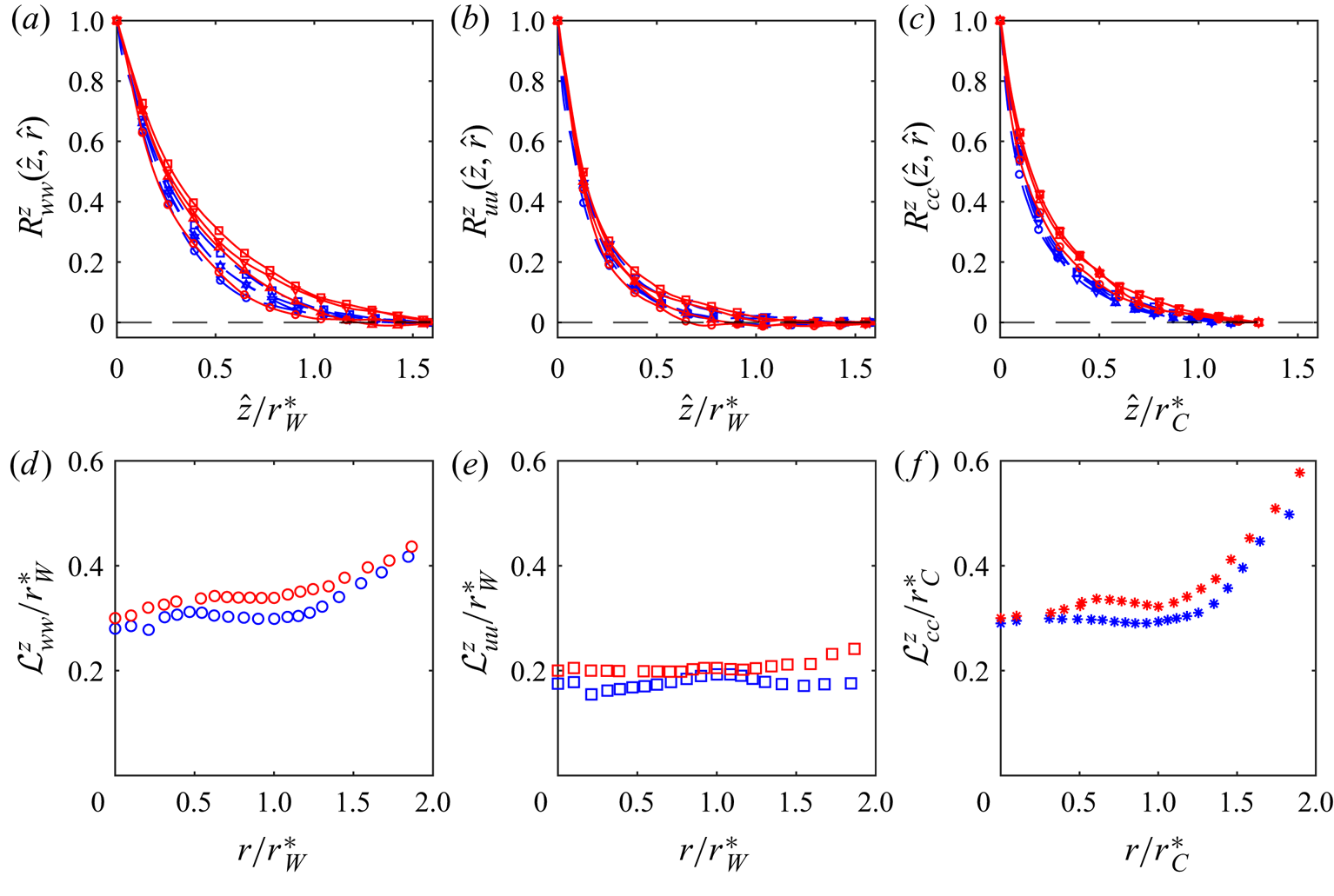
Finally, the results of  $R^{{{z}}}_{ii}(\hat {z}, \hat {r})$ at different radial locations are plotted in figure 8(a)–(c) for
 $\hat {r}/{r^\ast } = 0$, 0.6, 1.0 and 1.4 at
 $z/d = 30$ in the NJ and the NBJ. The associated integral length scale
 ${\mathcal {L}}^{z}_{ii}$ can be visually inferred from the area under the respective autocorrelation functions. It is observed that the integral length scale increases with distance from the axis. To confirm this, the distributions of integral length scale
 ${\mathcal {L}}^{z}_{ii}$ for
 $i = w, u, c$ obtained at several radial locations in the NJ and the NBJ are shown in figure 8(d)–(f). At a given axial location,
 ${\mathcal {L}}^{z}_{ii}$ increases with
 $r$ near the jet centreline, remains nominally constant for
 $0.7 \leq r/r^\ast \leq 1.3$ and then increases monotonically up to the edge of the jet. In an earlier study, Wygnanski & Fiedler (Reference Wygnanski and Fiedler1969) also reported that
 ${\mathcal {L}}^{z}_{ii}$ increased with
 $r$ monotonically in the NJ. Comparing the results in the NJ and the NBJ, we find that
 ${\mathcal {L}}^{z}_{ii}$ has similar shapes in both the flows when scaled by the local jet half-width, however, the normalised values
 ${\mathcal {L}}^{z}_{ii}/r^\ast$ are marginally higher in the middle and outer regions of the NBJ. These differences are possibly related to the different spreading rates of the NJ and the NBJ.
Autocorrelation functions of velocity and scalar concentration fluctuations (a)  $R^{{{z}}}_{ww}$, (b)
 $R^{{{z}}}_{uu}$ and (c)
 $R^{{{z}}}_{cc}$ at three radial locations
 $\hat {r}/{r^\ast } = 0$ (
 $\circ$), 0.6 (
 $\triangle$), 1.0 (
 $\triangledown$) and 1.4 (
 $\square$) in the NJ (blue symbols) and the NBJ (red symbols) measured at
 $z/d = 30$. (d)–(f) Integral length scale
 ${\mathcal {L}}^{z}_{ii}$ as a function of radial distance
 $r$ in the NJ and the NBJ.

4.2. In the radial direction, $R^{{{r}}}_{ii}$

Following the study of Wygnanski & Fiedler (Reference Wygnanski and Fiedler1969), we obtain the distributions of  $R^{{{r}}}_{ii}(\hat {z}, \hat {r})$ along the radial direction as per (4.1). Wygnanski & Fiedler (Reference Wygnanski and Fiedler1969) used time series velocity data and converted it into spatial domain using Taylor's hypothesis, but we do not make such assumptions since we have spatial data available.
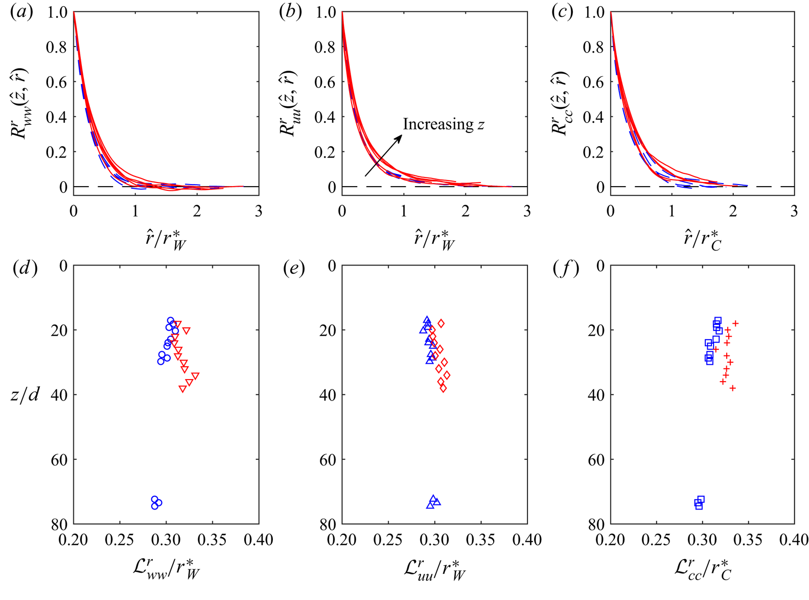
Figure 9(a)–(c) shows the autocorrelation functions  $R^{{{r}}}_{ww}$,
 $R^{{{r}}}_{uu}$ and
 $R^{{{r}}}_{cc}$ in the NJ and the NBJ as a function of radial separation distance,
 $\hat {r}$. The correlation functions are found to be similar when
 $\hat {r}$ is normalised by the corresponding jet half-widths,
 $r^\ast _{W}$ and
 $r^\ast _{C}$. This implies that the correlation functions
 $R^{{{r}}}_{ii}$ are becoming wider at the same rate as the growth of
 $r^\ast _{W}$ and
 $r^\ast _{C}$ in
 $z$. These findings suggest that the local length scales
 $r^\ast _{W}$ and
 $r^\ast _{C}$ are appropriate for scaling the correlation functions in both the NJ and the NBJ. For the NJ, the axial distance (
 $z$) is also a valid length scale since
 $r^\ast _{W}$ and
 $r^\ast _{C}$ have a linear growth in
 $z$, as previously observed in figure 4(b). In the NBJ, it is found that the similarity between
 $R^{{{r}}}_{cc}$ at different axial locations decreases with
 $z$. For instance, at
 $z/d \geq 38$, the normalised correlation functions are found to be wider in the NBJ compared with the correlation functions closer to the source. This is possibly due to turbulent scalar eddies peeling-off intermittently at the jet boundary as the local Froude number becomes very small.
Radial autocorrelation functions ( $R^{{{r}}}_{ii}$) of velocity and concentration fluctuations measured in the NJ and the NBJ: (a)
 $R^{{{r}}}_{ww}$, (b)
 $R^{{{r}}}_{uu}$ and (c)
 $R^{{{r}}}_{cc}$. Profiles of (d)
 ${\mathcal {L}}^{r}_{ww}$, (e)
 ${\mathcal {L}}^{r}_{uu}$ and (f)
 ${\mathcal {L}}^{r}_{cc}$ normalised with
 $r^\ast _{W}$ and
 $r^\ast _{C}$. Blue and red symbols represent the NJ and the NBJ results, respectively.

The radial integral length scale  ${\mathcal {L}}^{r}_{ii}$ of velocity and concentration fluctuations are calculated from the autocorrelation functions as
 \begin{equation} {\mathcal{L}}^{r}_{ii}(z) = \int_0^\infty {R^{{\hat{r}}}_{ii}(z,\hat{r})}\,\mathrm{d}\hat{r}; \quad i = w,u,c. \end{equation}
Note that the integral is evaluated in the same manner as the axial integral length scale. It is important to note that  ${\mathcal {L}}^{r}_{i}$ is a function of
 $z$ due to the growth of jet. The integral length scales
 ${\mathcal {L}}^{r}_{ii}$ for
 $i = w, u, c$ are plotted in figure 9(d)–(f), respectively. For the ease of comparison, the scale of the abscissa is kept the same in all the subplots. As indicated by blue symbols,
 ${\mathcal {L}}^{r}_{ii}/r^\ast$ for all
 $i$ in the NJ shows some initial variation with
 $z$ but eventually becomes constant. The same trends are seen in
 ${\mathcal {L}}^{r}_{ii}/r^\ast$ in the NBJ. However, the ratio is marginally higher in the NBJ when compared with the NJ, similar to the behaviour of axial integral length scales observed in the previous section. These results suggest the radial integral length scales
 ${\mathcal {L}}^{r}_{ii}$ in both the flows grow in proportion to the jet half-width, and the higher ratio of
 ${\mathcal {L}}^{r}_{ii}/r^\ast$ in the NBJ is mainly due to radial distribution of momentum and turbulence due to decelerated mean flow. As an interim conclusion based on axial and radial correlation length scales, we find that the turbulence structure is very similar in the NJ and the NBJ, and the relevant length scale is the local jet half-width.
5. Two-dimensional correlation map
Using the spatial information of velocity and concentration fluctuations, it is possible to quantify the organisation of turbulence structures via the two-point correlation map defined as
 \begin{equation} \varGamma_{{ii}}(\hat{z},\hat{r})|_{r^\prime} = \frac{\overline{i({{z^\prime},r^\prime}) i({z^\prime + \hat{z}, r^\prime+\hat{r}})}}{{\sigma_i({z^\prime}, r^\prime) \sigma_i ({z^\prime}+ \hat{z}, r^\prime+\hat{r})}},\quad i = w,u,c. \end{equation}
Here,  $\hat {r}$ represents the separation distance in the radial direction defined with respect to the reference location,
 $r^\prime$. Note that
 $z^\prime = 0$ in (5.1), and it represents the midsection of each measurement station. In the discussion below, we will compare the correlation maps at two locations, i.e. jet axis (
 $r^\prime = 0$) and jet edge (
 $r^\prime = r_s$). The location
 $r^\prime = r_s$ corresponds to the location close to edge of the jet, where the mean velocity is 1 % of the centreline value, i.e.
 ${W(r^\prime )}/{W_c} = 0.1$.
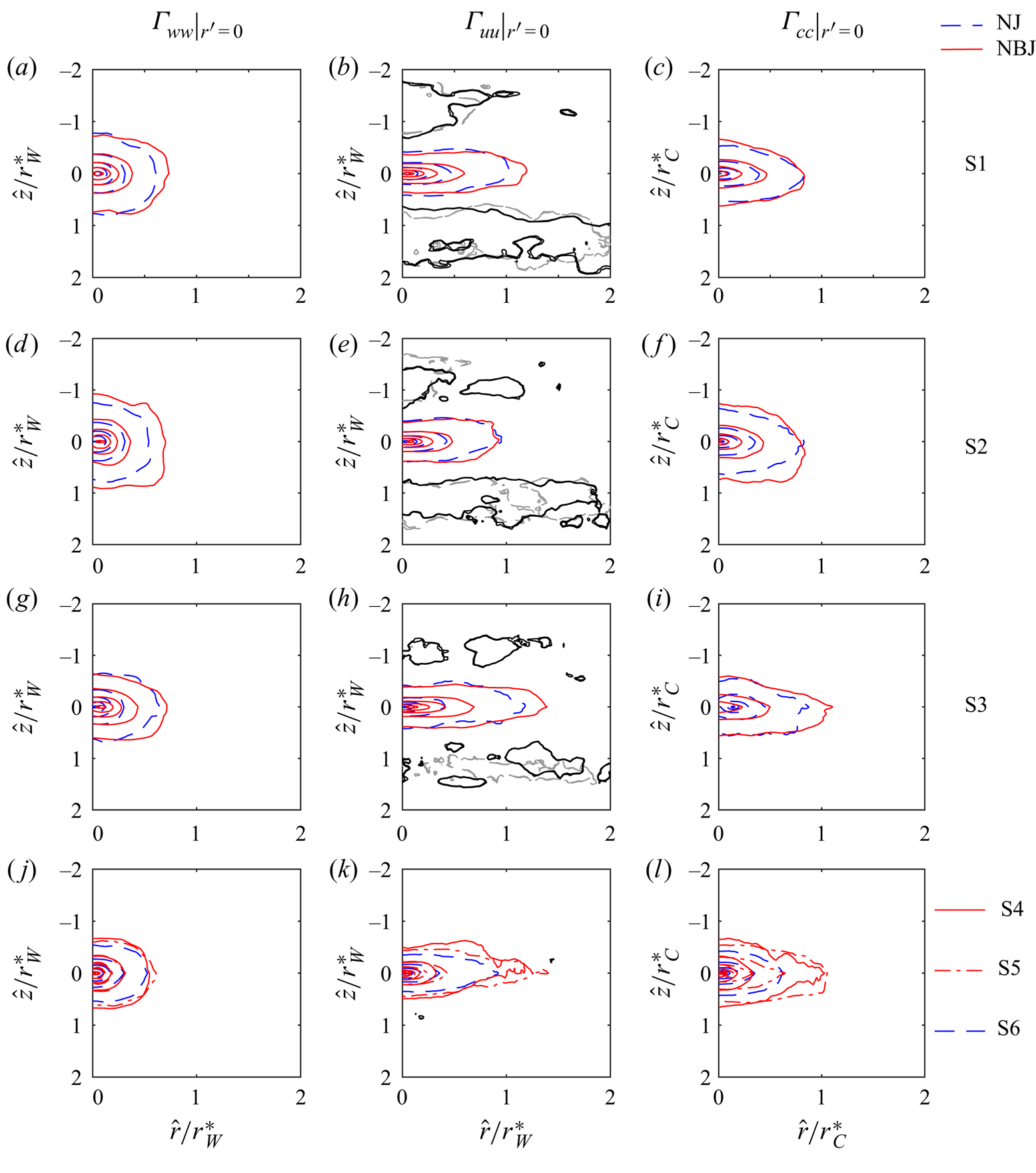
The results of  $\varGamma _{ii}|_{r^\prime =0}$ for
 $i = w, u, c$ at measurement locations S1 to S3 in the NJ and the NBJ are shown in figure 10(a)–(i). Note that the correlation maps are only shown on one side of the jet axis as the correlation maps of
 $\varGamma _{{ii}}|_{r^\prime =0}$ are symmetric about the jet axis. At first, a comparison of the results in figure 10 reveals that
 $\varGamma _{{ww}}|_{r^\prime =0}$ has a relatively larger length scale in the axial direction, while
 $\varGamma _{{uu}}|_{r^\prime =0}$ and
 $\varGamma _{{cc}}|_{r^\prime =0}$ have greater radial spread. The above result indicates clear anisotropy in the turbulent field as the axial velocity correlations are considerably longer than the radial velocity correlation, and with higher correlations. We also observe that the correlations of
 $u$ and
 $c$ in the NBJ are marginally wider in the radial direction in comparison with the NJ. This is because as the mean axial flow is slowed by negative buoyancy, the NBJ is forced to spread out radially in order to conserve the volume flux. Recently, Ezzamel, Salizzoni & Hunt (Reference Ezzamel, Salizzoni and Hunt2015) conducted an experimental study comparing the turbulence structure in a forced and a pure plume. They found similar results in a pure plume, wherein, the buoyancy causes marginally widening and elongation of the correlation maps of
 $w$ and
 $u$.
Spatial correlation map of the velocity and concentration fluctuations about the jet axis; (a,d,g)  $\varGamma _{{ww}}|_{r^\prime =0}$, (b,e,h)
 $\varGamma _{{uu}}|_{r^\prime =0}$ and (c,f,i)
 $\varGamma _{{cc}}|_{r^\prime =0}$ at measurement locations S1, S2 and S3, respectively. Red and blue contours represent NBJ and NJ, respectively. An additional contour (grey, NJ; black, NBJ) at
 $-0.01$ is shown for
 $\varGamma _{{uu}}$ in panels (b,e,h), panels (j,k,l) at stations S4 (red solid lines) and S5 (red dot-dashed lines) and S6 (blue dashed lines). Contour levels are from 0.1 to 0.9 in increments of 0.2.

Next, we find an alternating pattern of positive and negative contour regions in the correlation map of  $\varGamma _{{uu}}|_{r^\prime =0}$ in the axial direction, which consolidates our earlier observation that the jet is meandering or flapping about the jet axis near the source. As discussed before, the flapping of the jet is predominantly seen in transitional jets (List Reference List1982). In the present study, due to lower
 $Re$ in the NJ and the NBJ, some residual behaviour of transitional jets is observed here. Hence, the spatial correlation maps shown in figures 10(b), 10(e) and 10(h) will be slightly different in the NJ and the NBJ at higher
 $Re$. The length scale associated with the flapping is estimated as the distance between two adjacent negatively correlated regions and is found to be approximately 3
 $r^\ast _{W}$. It is worth noting that the width of negative contours decreases with
 $z$, in other words, the intensity of axisymmetric pulsing/flapping decreases with
 $z$.
Further, we find that the positive correlations of  $\varGamma _{{ii}}|_{r^\prime =0}$ for
 $i = w, u, c$ are limited to a radial distance of
 $\hat {r}/r^\ast \approx 0.8 \text {--} 1.1$. The above results indicate a rapid drop in the correlation value of velocity and scalar fluctuations in the radial direction in both the NJ and the NBJ. This implies a weak correlation between turbulence at the axis and the outer region of the jet. In other words, the radial transport of momentum and scalar fluxes is weaker at the jet axis in both the flows. This result is consistent with the behaviour of Reynolds stress in figure 5(c), and the radial scalar flux (
 $\overline {uc}$) is small near the jet axis (Milton-McGurk et al. Reference Milton-McGurk, Williamson, Armfield, Kirkpatrick and Talluru2020b). It is noticed that
 $\varGamma _{{ii}}|_{r^\prime =0}$ also dropped quickly in the axial direction within the region
 $-0.8 \leq \hat {z}/r^\ast \leq 0.8$. Despite some minor differences, the above results indicate that the turbulence structure in the NJ and the NBJ scale well with the local jet width.
Looking further, the correlation maps of  $\varGamma _{{ii}}|_{r^\prime =0}$ for
 $i = w, u, c$ at stations S4 (red dashed lines), S5 (solid red lines) in the NBJ and station S6 (blue dashed lines, self-similar NJ) in the NJ are plotted in figures 10(j), 10(k) and 10(l), respectively. There is a very good similarity between the correlation maps of
 $w, u, c$ fluctuations in the NJ and the NBJ at stations S1 to S3, when normalised by
 $r^\ast _{W}$ and
 $r^\ast _{C}$. These results suggest that the NBJ has a similar structure to that of the NJ with respect to the local jet width. Only minor differences are seen in
 $\varGamma _{{uu}}|_{r^\prime =0}$ and
 $\varGamma _{{cc}}|_{r^\prime =0}$ at stations S4 and S5, where the axial and radial length scales are marginally larger in the NBJ, consistent with our earlier observations about the integral length scales. Further, there is no alternating pattern of positive and negative correlations in
 $\varGamma _{{uu}}|_{r^\prime =0}$, which indicates that the flapping/meandering finally disappears beyond
 $z/d = 30$ at S4 and S5 (see figure 10k). Lastly, unlike the smooth contours of
 $\varGamma _{{ww}}$, the correlation maps
 $\varGamma _{{uu}}$ and
 $\varGamma _{{cc}}$ in the NBJ appear to be more uneven and irregular. This is possibly because of the intermittent peeling off of fluid in the outer region of the NBJ as buoyancy dominates over momentum near the jet boundary.
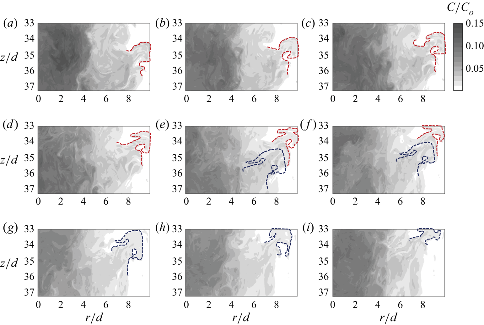
To explain this further, we show the instantaneous images of the concentration field in the NBJ at station S4 in figure 11(a)–(i), starting from  $t = 7\ \textrm {s}$ in increments of
 ${\rm \Delta} t = 0.285\ \textrm {s}$. In order to be consistent with the schematic in figure 1, all the subfigures are plotted such that the main jet is moving vertically downwards. A dashed curved line is drawn around the eddy to facilitate visual tracking of the movement of detached eddies at the jet boundary. At
 $t = 7$ s, an eddy (marked in red) begins to peel off from the NBJ, and when the momentum of fluid in the eddy is dominated by buoyancy forces, the eddy travels vertically upwards. This is clearly evident by tracking the movement of that eddy in figure 11(a–e). Finally, the eddy leaves the field of view in figure 11(f). Following this, we find a second eddy (marked as blue dashed curve) that is moving vertically upwards in figure 11(e–i). It should be noted that eddies peel-off only intermittently in the NBJ, although in this particular set of images, there is a continuous breaking of eddies. The above flow visualisation suggests that the uneven or rugged contours of
 $\varGamma _{{uu}}$ and
 $\varGamma _{{cc}}$ in the NBJ as seen in figure 10(k,l) is due to occasional detachment of buoyancy dominated eddies.
Flow visualisation of the NBJ at station S4 starting from (a)  $t = 7.0\ \textrm {s}$ and continuing in panels (b–i) in increments of
 ${\rm \Delta} t = 0.285\ \textrm {s}$. Note that the main jet is moving vertically downwards. The red and blue dashed curved lines are drawn to track the upward movement of detached eddies. Shading indicates normalised scalar concentration (
 $C/C_o$, where
 $C_o$ is the source concentration) as per the scale given top right.

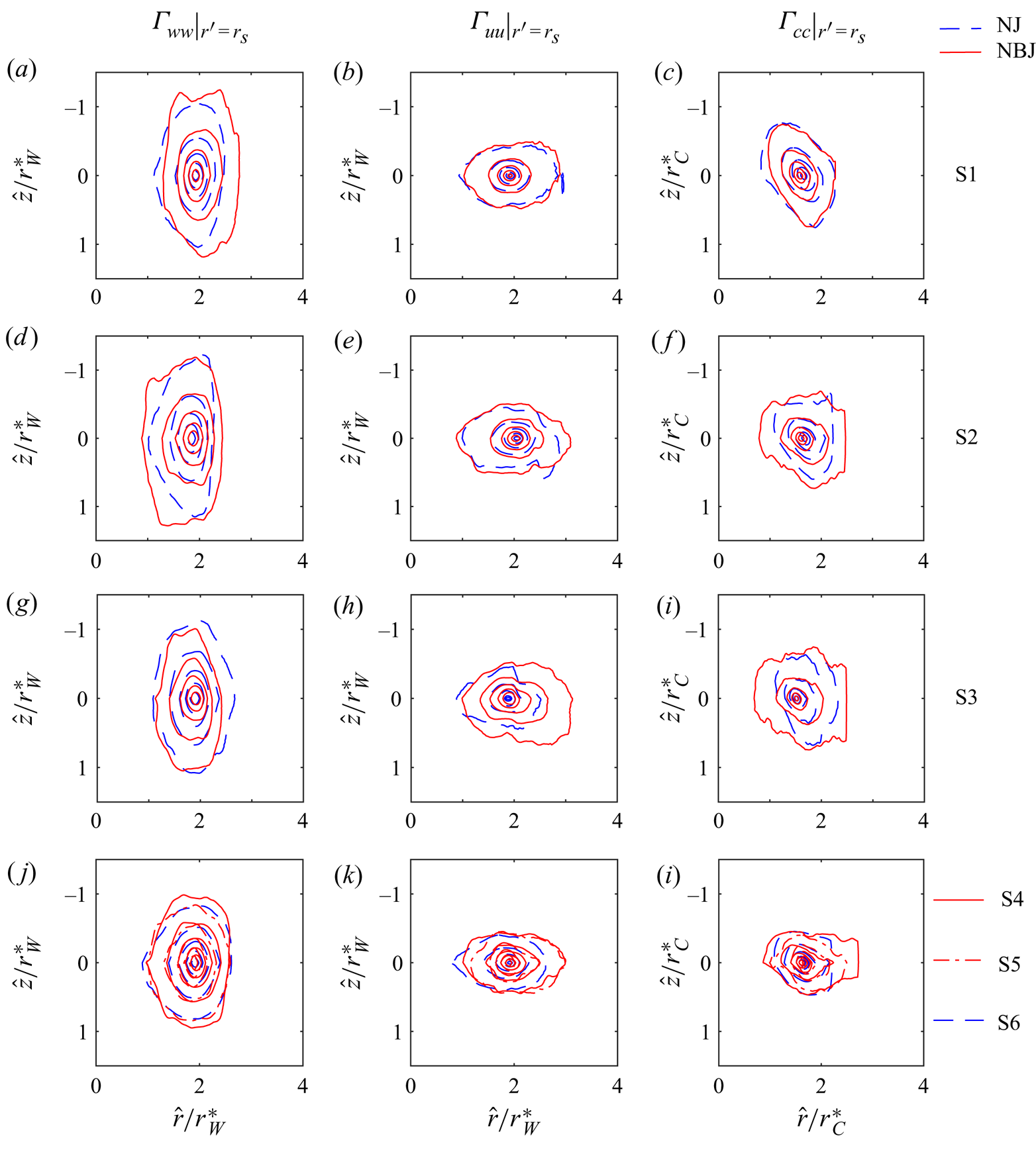
Figure 12 shows the correlation maps of  $\varGamma _{{ii}}$ for
 $i = w, u, c$ in the NJ and the NBJ computed at the jet edge (
 $r^\prime = r_s$) at measurement stations S1 to S6. The jet edge
 $r_s$ is defined as the location, where
 $W/W_c = 0.1$. Similar to the results of
 $\varGamma _{{ii}}$ at the centreline, we note that the axial length scales are larger in
 $\varGamma _{{ww}}|_{r^\prime =r_s}$, while
 $\varGamma _{{uu}}|_{r^\prime =r_s}$ and
 $\varGamma _{{cc}}|_{r^\prime =r_s}$ are wider in the radial direction in both the flows. Looking at the results in figure 12, we observe that the contour maps of
 $\varGamma _{{ww}}$,
 $\varGamma _{{uu}}$ and
 $\varGamma _{{cc}}$ are similar in the NJ and the NBJ at all measurement locations when normalised by the local jet half-widths,
 $r^\ast _{W}$ and
 $r^\ast _{C}$. Nonetheless, the distributions of
 $\varGamma _{{uu}}$ and
 $\varGamma _{{cc}}$ in the NBJ are marginally wider in the radial direction when compared with the NJ. This is possibly due to higher turbulent momentum and scalar fluxes in the radial direction of the NBJ.
Spatial correlation map of the velocity and concentration fluctuations about the jet edge; (a,d,g)  $\varGamma _{{ww}}|_{r^\prime =r_s}$, (b,e,h)
 $\varGamma _{{uu}}|_{r^\prime =r_s}$ and (c,f,i)
 $\varGamma _{{cc}}|_{r^\prime =r_s}$ at measurement locations S1, S2 and S3, respectively. Red and blue contours represent the NBJ and the NJ, respectively. (j,k,l) At stations S4 (red solid lines) and S5 (red dot-dashed lines) and S6 (blue dashed lines); contour levels are from 0.1 to 0.85 in increments of 0.25.

As an interim conclusion, the discussion of two-dimensional correlations reveals that although the centreline quantities ( $W_c$ and
 $C_c$) and the corresponding half-widths (
 $r^\ast _{W}$ and
 $r^\ast _{C}$) vary differently along
 $z$ in the NJ and the NBJ, the turbulence structure, nonetheless, remains similar in both the flows when scaled by the local length scales. This further consolidates our earlier finding that the effect of negative buoyancy in the NBJ is primarily seen on the length and velocity scales in the mean flow.
6. Spectra
In this section, we will look at the contribution of different frequencies to the energy spectra of  $w$,
 $u$ and
 $c$ in the NJ and the NBJ. The spectral density in the axial direction,
 $S^{{{z}}}_{ii}$ and the corresponding autocorrelation function
 $R^{{\hat {z}}}_{ii}$ are related as they are Fourier transform pairs. For instance,
 $S^{{{z}}}_{ii}$ is related to
 $R^{{\hat {z}}}_{ii}$ as
 \begin{equation} S^{{{z}}}_{ii}(k_z) = \frac{1}{2{\rm \pi}} \int^{\infty}_{-\infty} R^{{\hat{z}}}_{ii}(\hat{z}) \,\textrm{e}^{-jk_z\hat{z}} \,\mathrm{d}\hat{z},\quad i = w,u, c.\end{equation}
Here  $j$ represents the imaginary unit and
 $k_z$ is the wavenumber defined as
 $k_z = 2{\rm \pi} /\lambda _z$, where
 $\lambda _z$ is the wavelength. For a proper comparison of
 $S^{{{z}}}_{ii}$, it is scaled in a way that the area under the normalised spectra
 $\varPhi ^{{{z}}}_{ii}$ and
 $k_z$ is unity, i.e.
 $\varPhi ^{{{z}}}_{ii} = S^{{{z}}}_{ii}/\sigma ^2_{i}$, where
 $\sigma ^2_i$ is the variance of a physical quantity
 $i$.
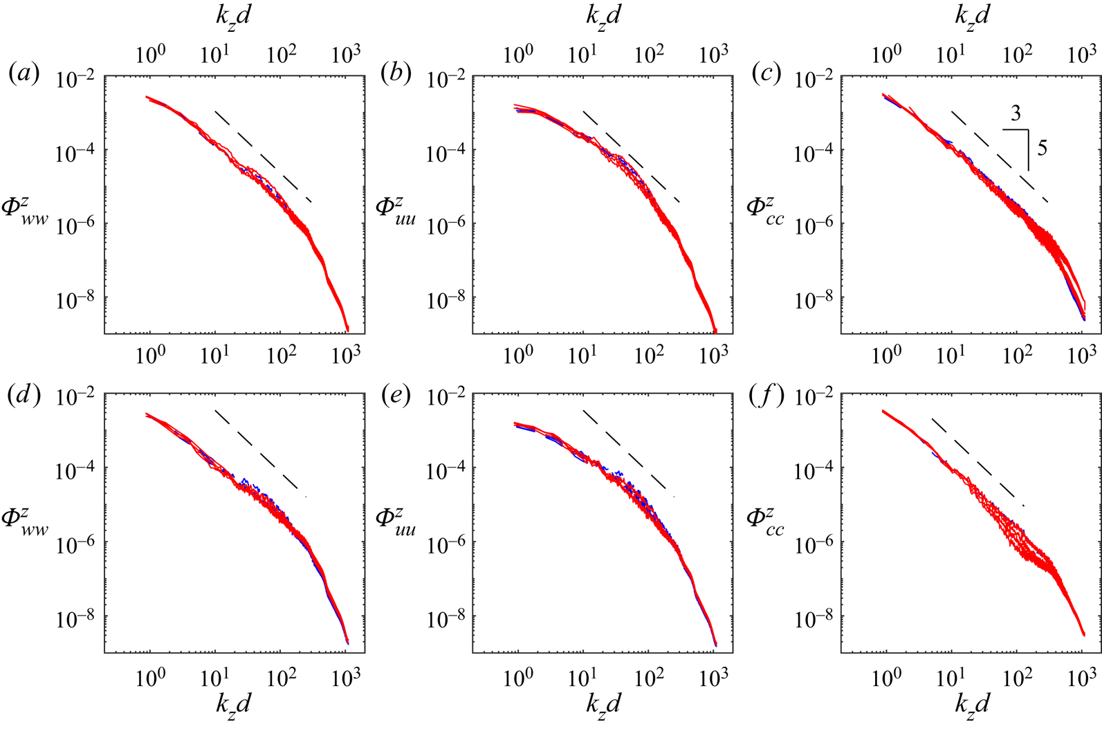
At first, we present the results of  $\varPhi ^{z}_{ii}$ on the jet axis in figure 13(a)–(c) for
 $i = w$,
 $u$ and
 $c$ measured at
 $z/d = 18$, 23, 28 and 76 in the NJ, and
 $z/d = 19$, 24, 28, 35 and 38 in the NBJ. The blue dashed and red solid lines in the figure 13 represent the spectra in the NJ and the NBJ, respectively. It is a clear that
 ${\varPhi ^{z}_{ii}}$ in the NBJ is similar to those in the NJ for
 $w$,
 $u$ and
 $c$ at all locations. This result suggests that although the turbulence intensities of
 $w$,
 $u$ and
 $c$ (when normalised with
 $W_c$ and
 $C_c$) are different in the NJ and the NBJ (refer to figure 5), the normalised spectra is nonetheless similar. In physical terms, this result indicates that the range of turbulence length scales on the jet axis in the NBJ is not affected by negative buoyancy, but there is still an effect on the largest scale (i.e. jet width) due to decelerated mean flow.
(a)–(c) Normalised spectra ( $\varPhi ^{{{z}}}_{ii}$) of velocity and concentration fluctuations measured on the jet centreline at
 $z/d = 18$, 23, 28 and 76 in the NJ, and
 $z/d = 19$, 24, 28, 35 and 38 in the NBJ plotted as a function of normalised axial wavenumber
 $k_z d$. (d)–(f) Here
 $\varPhi ^{{{z}}}_{ii}$ at four radial locations,
 $r/{r^\ast } = 0$, 0.6, 1.0 and 1.4 at
 $z/d = 30$: (a,d)
 $\varPhi ^{z}_{ww}$, (b,e)
 $\varPhi ^{z}_{uu}$ and (c,f)
 $\varPhi ^{z}_{cc}$. The dashed lines represent the
 $-5/3$ slope in the inertial region of the spectra. Blue dashed and red solid lines represent the NJ and the NBJ, respectively.

Further, all the spectra have an approximate  $-5/3$ slope in the intermediate range of scales. Of the three spectra,
 $\varPhi ^{z}_{cc}$ has a better agreement with the
 $-5/3$ slope compared with
 $\varPhi ^{z}_{ww}$ and
 $\varPhi ^{z}_{uu}$, which indicates that the scalar is more homogeneously mixed than
 $w$ and
 $u$. For further comparison, the results of normalised spectra of velocity and concentration fluctuations in the NJ and the NBJ at
 $z/d = 30$ are plotted in figure 13(d)–(f) at four radial locations,
 $r/{r^\ast } = 0$, 0.6, 1.0 and 1.4. There are no quantifiable differences in the spectra of
 $w$,
 $u$ and
 $c$ between the NJ and the NBJ at all radial locations. The minor differences in the concentration spectra at the axis and off-axis locations in the NBJ in figure 13(f) are within the experimental error in estimating the concentration spectra. Overall, the good agreement between the spectra of
 $w$,
 $u$ and
 $c$ at the jet centreline and other radial locations in both the flows further confirm our earlier discussion that the turbulence structure in the NJ and the NBJ is very similar, despite the effect of negative buoyancy on the mean flow.
7. Probability density functions
In this section, we will examine how negative buoyancy affects the probability density functions of velocity and concentration in the NJ and the NBJ. In general, the probability  ${\mathcal {P}}(\tilde {W}, \tilde {W}+ \textrm {d}\tilde {W})$ of a fluctuating velocity signal in the interval
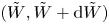 $(\tilde {W}, \tilde {W}+ \textrm {d}\tilde {W})$ is the ratio of the number of velocity data points that occur in this interval divided by the total number of data points recorded. The p.d.f. for this interval is then defined as the ratio
 ${{\mathcal {P}}(\tilde {W}, \tilde {W}+ \textrm {d}\tilde {W})}/{\textrm {d}\tilde {W}}$. Note that
 $\tilde {W}$ represents the instantaneous axial velocity. For proper comparison of results, the p.d.f. (
 ${\mathcal {P}}_{\tilde {W}}$) is normalised such that the area under the curve is unity, i.e. the integral
 $\int {\mathcal {P}}_{\tilde {W}} \,\textrm {d}(\tilde {W}/W_o) = 1$. We define
 ${\mathcal {P}}_{\tilde {W}}$ and
 ${\mathcal {P}}_{\tilde {C}}$ in a similar manner.
7.1. Jet centreline
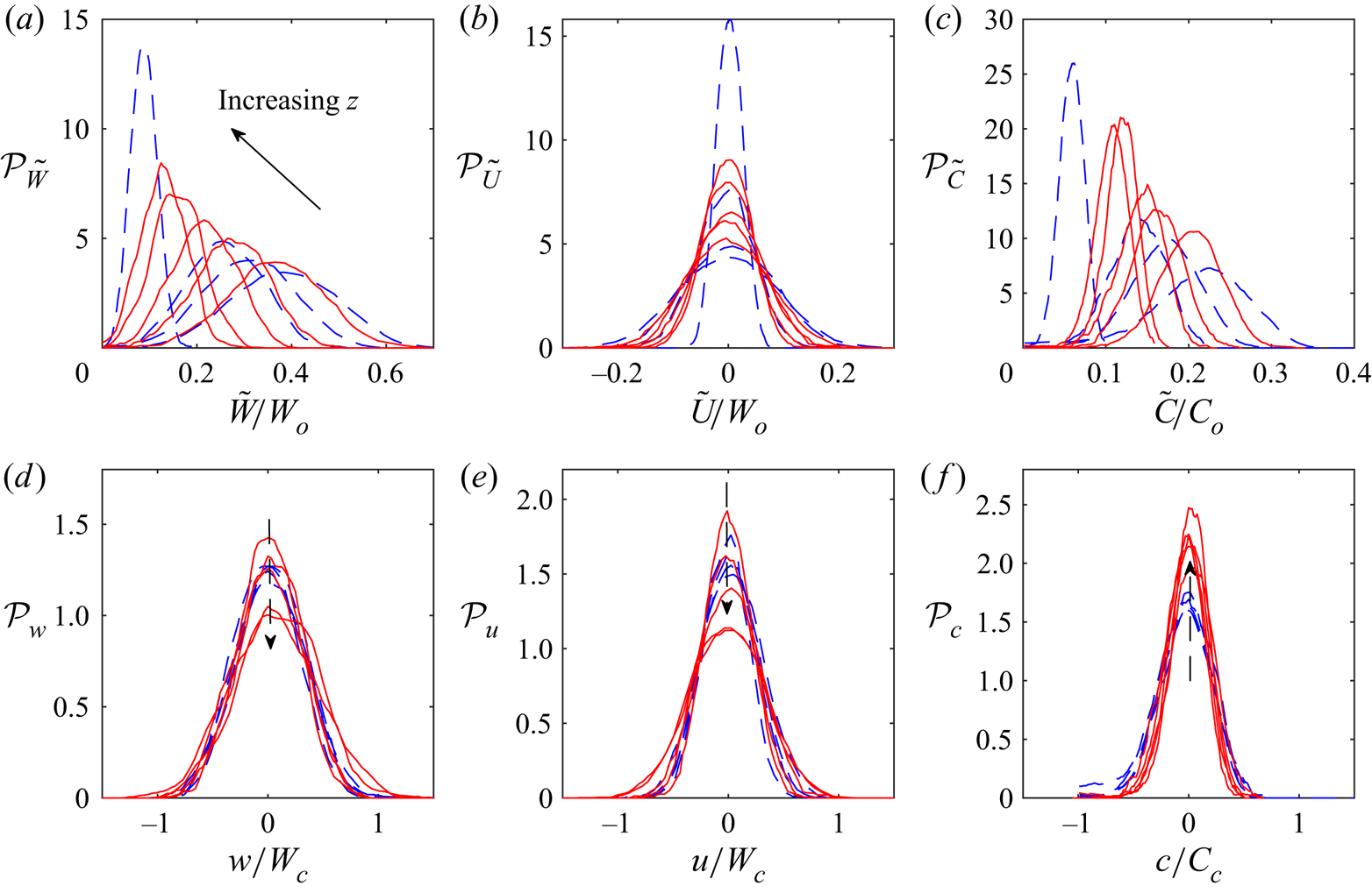
Figure 14(a)–(c) shows the results of  ${\mathcal {P}}_{\tilde {W}}$,
 ${\mathcal {P}}_{\tilde {U}}$ and
 ${\mathcal {P}}_{\tilde {C}}$ on the jet axis at
 $z/d$ = 18, 23, 28 and 76 in the NJ, and
 $z/d = 19$, 24, 28, 35 and 38 in the NBJ. In this representation, we see that the distributions of
 ${\mathcal {P}}_{\tilde {W}}$ and
 ${\mathcal {P}}_{\tilde {C}}$ shift to the left as expected, whereas
 ${\mathcal {P}}_{\tilde {U}}$ is uniformly distributed about the zero line. Due to deceleration of the mean flow, the profiles of
 ${\mathcal {P}}_{\tilde {W}}$ in the NBJ shift towards the zero line faster than those in the NJ at similar
 $z/d$ values. In contrast, the shift of
 ${\mathcal {P}}_c$ towards the zero line is slower in the NBJ as there is stagnation of the scalar in the axial direction due to decelerated mean flow. Importantly, we observe that
 ${\mathcal {P}}_{\tilde {W}}$,
 ${\mathcal {P}}_{\tilde {U}}$ and
 ${\mathcal {P}}_{\tilde {C}}$ in the NJ and the NBJ have Gaussian shapes about their respective mean values, and the p.d.f.s become narrower with
 $z$. The width of the Gaussian curves, which is equal to
 $\sigma _i$, decreases with
 $z$ in both the flows. Comparing the distributions of
 ${\mathcal {P}}_{\tilde {W}}$,
 ${\mathcal {P}}_{\tilde {U}}$ and
 ${\mathcal {P}}_{\tilde {C}}$ at similar
 $z/d$ values in the NJ and the NBJ, we find that although the profiles are relatively shifted, the widths of the p.d.f.s are quite similar. This indicates that the magnitudes of turbulent fluctuations (i.e.
 $\sigma _w/W_o$,
 $\sigma _u/W_o$ and
 $\sigma _c/U_o$ in figure 6) in the NBJ are similar to those in the NJ.
Probability density functions of (a)  ${\mathcal {P}}_{\tilde {W}}$, (b)
 ${\mathcal {P}}_{\tilde {U}}$ and (c)
 ${\mathcal {P}}_{\tilde {C}}$ on the jet centreline at
 $z/d = 18$, 23, 28 and 76 in the NJ, and
 $z/d = 19$, 24, 28, 35 and 38 in the NBJ. Here, the source velocity (
 $W_o$) and concentration (
 $C_o$) are used for normalisation. (d)–(f) The p.d.f.s of velocity and concentration fluctuations (
 ${\mathcal {P}}_w$,
 ${\mathcal {P}}_u$ and
 ${\mathcal {P}}_c$) normalised by the local centreline velocity (
 $W_c$) and concentration (
 $C_c$). The vertical arrows in panels (d)–(f) indicate the direction of increasing
 $z$. Blue dashed and red solid lines represent the NJ and the NBJ, respectively.

Figure 14(d)–(f) shows the p.d.f.s ( ${\mathcal {P}}_{w}$,
 ${\mathcal {P}}_{u}$ and
 ${\mathcal {P}}_{c}$) of velocity and concentration fluctuations on the jet axis. Some differences can be observed between the NJ and the NBJ. First, the distributions of
 ${\mathcal {P}}_{w}$,
 ${\mathcal {P}}_{u}$ and
 ${\mathcal {P}}_{c}$ in the NJ show self-similar behaviour when the turbulent fluctuations are normalised by the local centreline mean velocity and concentration. This indicates that both the mean and turbulence quantities in the NJ scale with the local centreline velocity and concentration. In contrast, such similarity is not seen in the NBJ because the turbulent fluctuations do not scale with
 $W_c$ and
 $C_c$, as previously observed. Secondly, the peak values of
 ${\mathcal {P}}_{w}$ and
 ${\mathcal {P}}_{u}$ for the NBJ decrease with
 $z$, while the peak in
 ${\mathcal {P}}_{c}$ increases with
 $z$.
7.2. In the radial direction
The distributions of  ${\mathcal {P}}_{\tilde {W}}$,
 ${\mathcal {P}}_{\tilde {U}}$ and
 ${\mathcal {P}}_{\tilde {C}}$ at
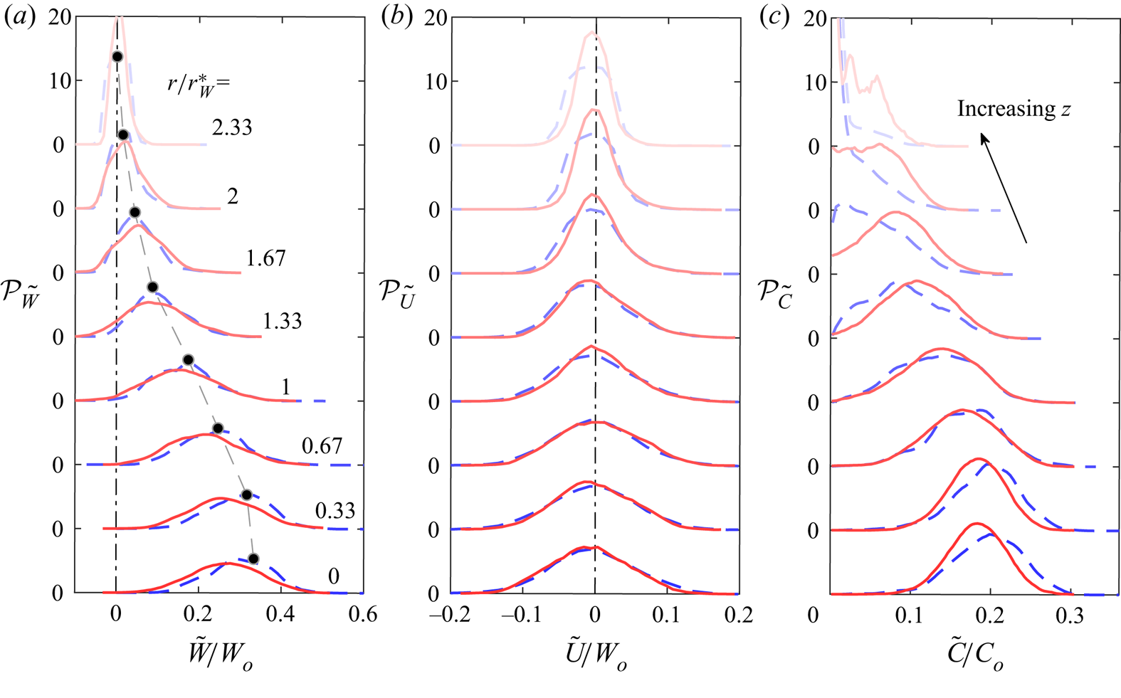
 $z/d = 30$ in the NJ and the NBJ are shown in figure 15(a)–(c). In each subplot, the results at eight radial locations
 $r/r^\ast _W = 0$, 0.33, 0.67, 1, 1.33 1.67, 2 and 2.33 are shown from bottom to top, respectively. For clarity, the curves at different radial locations are shifted up vertically by 10 units. Some salient observations can be made here.
Probability density functions measured at station S3: (a)  ${\mathcal {P}}_{\tilde {W}}$, (b)
 ${\mathcal {P}}_{\tilde {U}}$ and (c)
 ${\mathcal {P}}_{\tilde {C}}$ at radial distances
 $r/r^\ast _W = 0, 0.33, 0.67,\ldots , 2.33$ as indicated by different shades of blue dashed (NJ) and red solid (NBJ) lines. The curves at increasing
 $r/r^\ast _W$ are shifted vertically by 10 units. The dashed grey line in panel (a) is the locus of the mean value of
 $\tilde {W}$ in the NJ at different radial distances. The vertical dot-dashed lines in panel (a) and panel (b) show the zero values of
 $\tilde {W}$ and
 $\tilde {U}$, respectively.

(i) Looking at the distributions of  ${\mathcal {P}}_{\tilde {W}}$, it is clear that the curves in the NJ are Gaussian for
 $r/r^\ast _W \leq 1.67$, while the profiles of
 ${\mathcal {P}}_{\tilde {W}}$ in the NBJ are clearly skewed even at small radial locations (blue dashed curves). The horizontal shift of the peak values resembles the Gaussian profile of mean velocity, which is indicated by the grey dashed line in figure 15(a) for the NJ. Further, the varying width of the Gaussian curves closely follows the variation of
 $\sigma _w/W_c$ (in figure 5) in the radial direction, reaching a maximum around
 $r/r^\ast _W = 0.67$. At all
 $r$ locations, we find that
 ${\mathcal {P}}_{\tilde {W}}$ in the NBJ and the NJ are similar with a systematic shift in the profiles. Closer to the jet axis,
 ${\mathcal {P}}_{\tilde {W}}$ in the NBJ is shifted slightly to the left, which is because of the mean flow being slowed down by negative buoyancy. On the other hand, the profiles of
 ${\mathcal {P}}_{\tilde {U}}$ in the NJ and the NBJ shown in figure 15(b) are practically identical. They have Gaussian shapes at all
 $r$-locations, except at the jet boundary, where
 ${\mathcal {P}}_{\tilde {U}}$ in the NJ is positively skewed whereas it is Gaussian in the NBJ.
(ii) Similar to the distributions of  ${\mathcal {P}}_{\tilde {W}}$, the shape of
 ${\mathcal {P}}_{\tilde {C}}$ changes with distance from the jet axis. Near the centreline,
 ${\mathcal {P}}_{\tilde {C}}$ is Gaussian, and it remains Gaussian up to
 $r/r^\ast _W = 1$ in the NJ. Beyond this radial location,
 ${\mathcal {P}}_{\tilde {C}}$ becomes asymmetrical due to intermittency in the flow and the shape resembles a gamma function. Further, the profiles of
 ${\mathcal {P}}_{\tilde {C}}$ shift towards the zero line in a Gaussian fashion. Lastly, the behaviour of
 ${\mathcal {P}}_{\tilde {C}}$ in the NBJ exhibits a key difference in comparison with the NJ. The shape of
 ${\mathcal {P}}_{\tilde {C}}$ remains Gaussian for greater radial distances in the NBJ. This may be explained as follows. In our experiments, we found that the axial flow in the NBJ is decelerated more rapidly due to negative buoyancy, and due to the continuity equation, the flow is forced to spread out radially. Further, the results of correlation functions and integral length scales in this study suggest that the turbulent structures fill up the jet more homogeneously, resulting in the Gaussian distributions of
 ${\mathcal {P}}_{\tilde {C}}$ in the NBJ.
8. Conclusions
We started this study by posing a question: ‘Is there any difference in the turbulence structure between the NJ and the NBJ?’, because some differences in the jet spreading rate, the entrainment rate and the scaling of turbulence stresses were reported in previous studies (Kaminski et al. Reference Kaminski, Tait and Carazzo2005; Papanicolaou et al. Reference Papanicolaou, Papakonstantis and Christodoulou2008; Milton-McGurk et al. Reference Milton-McGurk, Williamson, Armfield, Kirkpatrick and Talluru2020b). Our main objective was to understand how the previously reported differences may impact the turbulence structure in the NBJ. To this end, we obtained detailed spatial measurements of velocity and concentration using PIV and LIF measurement techniques. Analysis of correlation functions, spectra, integral length scales and the probability density functions have led to the following conclusions.
(i) The comparison of turbulence intensities and Reynolds stress in the NJ and the NBJ indicates that the effect of negative buoyancy is mainly on the mean flow. The apparent differences in the turbulence intensities between the NJ and the NBJ are because of using the local centreline velocity ( $W_c$) for scaling the statistics. For example,
 $W_c$ has a faster decay rate in the NBJ compared with the NJ and so, the normalised velocity turbulence intensities are relatively higher in the NBJ. In contrast, the normalised intensity of concentration fluctuations is lower in the NBJ as
 $C_c$ is higher than the NJ at similar
 $z/d$ values.
(ii) It is observed that the axial and radial integral length scales in the NJ and the NBJ scale very well with the local jet-width. In both the flows, the ratio of integral length scale and the jet half-width ( ${\mathcal {L}}^{r}_{ii}/r^\ast$,
 $i = w, u, c$) remains almost constant with
 $z$. Nonetheless, the two-dimensional correlation maps of
 $u$ and
 $c$ in the NBJ are observed to be elongated in the radial direction in comparison with the NJ, and these differences are explained in terms of the intermittent peel-off of fluid parcels at the jet boundary in the NBJ.
(iii) Comparing the spectra at different axial and radial locations in the NBJ, we found that there is excellent agreement between the NJ and the NBJ at all length scales. Only minor differences (within the limit of experimental error) are noticed in the concentration spectra with increasing distance from the jet axis.
(iv) The p.d.f.s of  $w$,
 $u$ and
 $c$ in the NJ and NBJ have similar Gaussian distributions across most parts of the jet. The differences in
 ${\mathcal {P}}_c$ between the NJ and the NBJ seen near the jet boundary are due to homogeneous distribution of turbulence in the NBJ as the mean axial flow is decelerated by negative buoyancy and the flow is pushed out radially in order to satisfy the constraint of continuity in the flow.
As a more general concluding remark, it is possible to say that negative buoyancy affects mainly the mean flow in the NBJ, and yet the mean velocity profile exhibits a self-similar Gaussian form when scaled using local centreline velocity and jet width. We also observe that negative buoyancy affects the large-scale eddies (of the size of the jet width) in the flow and causes the NBJ to spread more rapidly. Nonetheless, the turbulence structure remains similar in the NJ and the NBJ with respect to the local length scale, i.e. the local jet width. Although the flow conditions in the NBJ are rapidly changing, the turbulence stresses vary at a different rate compared with the mean velocity, and some differences are seen at the jet boundary, none of these differences seem to have a significant effect on the internal turbulence structure of the NBJ.
Acknowledgements
The authors acknowledge the Australian Research Council for its financial support.
Declaration of interests
The authors report no conflict of interest.