



1 Introduction
Gravity currents occur when a fluid propagates horizontally along a base (or along a ceiling) into another fluid with a different density (see, e.g. Simpson Reference Simpson1982; Huppert Reference Huppert1982b
; Gratton & Minotti Reference Gratton and Minotti1990; Huppert & Woods Reference Huppert and Woods1995; Ungarish & Huppert Reference Ungarish and Huppert2000; Hallez & Magnaudet Reference Hallez and Magnaudet2009; Zheng, Rongy & Stone Reference Zheng, Rongy and Stone2015b
); of course, similar dynamics can occur along inclined boundaries (see, e.g. Huppert Reference Huppert1982a
; Lister Reference Lister1992; Vella & Huppert Reference Vella and Huppert2006). One special case is the gravity current flowing over a permeable porous medium, where fluid loss occurs due to various drainage mechanisms, such as buoyancy and capillarity. This situation exists in everyday life, such as liquid droplets spreading on paper (see, e.g. Gillespie Reference Gillespie1958; Borhan & Rungta Reference Borhan and Rungta1992; Clarke et al.
Reference Clarke, Blake, Carruthers and Woodward2002), or in industrial processes, such as
 $\text{CO}_{2}$
leakage through a permeable caprock in a geological sequestration project (see, e.g. Pritchard, Woods & Hogg Reference Pritchard, Woods and Hogg2001; Neufeld & Huppert Reference Neufeld and Huppert2009) or in geological processes, such as the motion of the brackish water currents over the permeable bottom of estuaries (see, e.g. Thomas, Marino & Linden Reference Thomas, Marino and Linden1998; Ungarish & Huppert Reference Ungarish and Huppert2000).
Many previous studies in this context have focused on the buoyancy-driven fluid drainage from a propagating gravity current. For example, Thomas et al. (Reference Thomas, Marino and Linden1998) and Ungarish & Huppert (Reference Ungarish and Huppert2000) have studied the inertial gravity currents with buoyancy-driven drainage. For viscous gravity currents, Acton, Huppert & Worster (Reference Acton, Huppert and Worster2001) studied a gravity current spreading on and seeping into an infinitely deep porous medium, purely driven by gravitational forces. On the other hand, when the porous medium is of finite thickness, the problem has been studied, for example, by Davis & Hocking (Reference Davis and Hocking1999) and Pritchard et al. (Reference Pritchard, Woods and Hogg2001) for the case of an outward spreading current, and by Zheng, Shin & Stone (Reference Zheng, Shin and Stone2015c ) for the case of an inward spreading current. Other buoyancy-driven drainage situations may occur when there is a fault within the base (see, e.g. Neufeld et al. Reference Neufeld, Vella, Huppert and Lister2011; Vella et al. Reference Vella, Neufeld, Huppert and Lister2011), or there exists an edge (see, e.g. Zheng et al. Reference Zheng, Soh, Huppert and Stone2013). In addition, Yu, Zheng & Stone (Reference Yu, Zheng and Stone2016) recently studied the drainage of a viscous gravity current through both a permeable substrate and a fixed edge.
Another important situation occurs when the fluid drainage from a spreading gravity current is driven by the capillary forces, such as when a permeable substrate is wettable by the fluid. Several previous studies have investigated the capillary effects on the gravity current. For example, Woods & Farcas (Reference Woods and Farcas2009) and Sayag & Neufeld (Reference Sayag and Neufeld2016) investigated the effects of the capillary entry pressure on the leakage through a permeable rock, which is non-wettable by the spreading fluid. Also, there are studies of capillary retention, i.e. a certain amount of fluid is left inside the porous medium, through which the main current has passed, due to the capillary effects (Kochina, Mikhailov & Filinov Reference Kochina, Mikhailov and Filinov1983; Hesse, Orr Jr & Tchelepi Reference Hesse, Orr and Tchelepi2008; Farcas & Woods Reference Farcas and Woods2009; Juanes, MacMinn & Szulczewski Reference Juanes, MacMinn and Szulczewski2010; MacMinn et al. Reference MacMinn, Christopher, Szulczewski and Juanes2010; MacMinn, Szulczewski & Juanes Reference MacMinn, Szulczewski and Juanes2011; Nordbotten & Dahle Reference Nordbotten and Dahle2011). In addition, the problem of two-phase gravity currents due to the action of the capillary forces has been investigated by Golding et al. (Reference Golding, Neufeld, Hesse and Huppert2011), Golding, Huppert & Neufeld (Reference Golding, Huppert and Neufeld2013). However, the effects of the capillary-driven drainage is still an open question.
In this paper, we study the drainage of a viscous gravity current into a deep porous medium, where the motion is driven by both the gravitational and capillary forces. In particular, we emphasize the influence of the capillary effects on the dynamic behaviours of the current. First, we establish a one-dimensional drainage model in § 2, considering that a fluid drains into a deep porous medium in the vertical direction. Then, in § 3, we investigate the two-dimensional problem where a viscous gravity current drains vertically into a deep porous medium while horizontally spreading over the medium. For the two-dimensional problem, since there are no self-similar solutions for the entire time period, we investigate the early-time (§ 3.3) and the late-time (§ 3.4) asymptotic behaviours where self-similar solutions are available. We also numerically solve the governing partial differential equations to verify the self-similar solutions in the asymptotic limits, and to study the time transition between the early-time and the late-time asymptotic behaviours in § 3.5. In addition, we highlight the influence of the capillary effects for the two-dimensional problem (§ 4) and study the time transition between the early-time and the late-time self-similar behaviours. Finally, we close our paper in § 5 with some final remarks.
We note that the flow considered here has a dense liquid flowing over a less dense fluid (a gas phase in the porous media). Thus, it is natural to expect that a Rayleigh–Taylor-type instability can occur within the porous material and transverse to the main flow direction of the gravity current. Such gravitational instabilities were noticed in the experiments of Acton et al. (Reference Acton, Huppert and Worster2001) at relatively long times (the late-time period) and so there was a large time period over which the standard gravity current analysis rationalized the spreading. This gravitational instability has also been studied experimentally (see, e.g. Saffman & Taylor Reference Saffman and Taylor1958; Neufeld et al. Reference Neufeld, Hesse, Riaz, Hallworth, Tchelepi and Huppert2010; MacMinn et al. Reference MacMinn, Neufeld, Hesse and Huppert2012; Huppert, Neufeld & Strandkvist Reference Huppert, Neufeld and Strandkvist2013; Tsai, Riesing & Stone Reference Tsai, Riesing and Stone2013) and numerically and theoretically (see, e.g. Hewitt, Neufeld & Lister Reference Hewitt, Neufeld and Lister2013). In the early-time period, where the capillary effects are important, as discussed below, it is then safe to neglect the gravitational instability.
2 One-dimensional drainage
In order to address the two-dimensional problem of a viscous gravity current draining into a deep porous medium, we first consider a one-dimensional configuration sketched in figure 1. An infinitely deep porous medium with uniform porosity
 $\unicode[STIX]{x1D719}$
and permeability
 $k$
lies below
 $z=0$
. Liquid initially placed on top of the material drains into the porous medium, driven by both the gravitational and capillary forces. We are interested in the height of the liquid
 $h(t)$
above the porous medium and the depth of the liquid
 $\ell (t)$
penetrating into the porous medium, as functions of time
 $t$
. Here, we neglect the possibility of any instability that would destroy the one-dimensional drainage scenario.
Two situations are considered here: (i) the liquid is of a fixed volume, with an initial height
 $h_{0}$
; (ii) the liquid is continually added into the system above the porous medium, with the total volume
 $V$
as a function of
 $t$
given by
 $$\begin{eqnarray}V=qt^{\unicode[STIX]{x1D6FC}},\end{eqnarray}$$
where
 $q$
and
 $\unicode[STIX]{x1D6FC}$
are constants. In particular,
 $\unicode[STIX]{x1D6FC}=0$
and
 $1$
indicate, respectively, the cases of a fixed-volume release and constant-rate addition.
Sketch of the configuration of one-dimensional drainage of a liquid with density
 $\unicode[STIX]{x1D70C}$
and viscosity
 $\unicode[STIX]{x1D707}$
into a infinitely deep porous medium with porosity
 $\unicode[STIX]{x1D719}$
and permeability
 $k$
driven by both the gravitational and capillary forces. The vertical axis is denoted by
 $z$
and the top of the porous medium is located at
 $z=0$
. The height and the depth of the liquid above and inside the porous medium are denoted by
 $h$
and
 $\ell$
, respectively. The pressure distribution given by (2.5) is shown on the right. The inset highlights the enhanced drainage caused by the capillary forces.

In the liquid above the porous medium, the pressure
 $p(z,t)$
can be assumed to be hydrostatic and hence is given by
 $$\begin{eqnarray}p(z,t)=p_{0}+\unicode[STIX]{x1D70C}g(h-z),\quad \text{for}~0\leqslant z\leqslant h(t),\end{eqnarray}$$
where
 $p_{0}$
is the atmospheric pressure at the top of the liquid layer,
 $\unicode[STIX]{x1D70C}$
is the density of the liquid and
 $g$
is gravitational acceleration. In the porous medium, neglecting the inertial effects, Darcy’s law yields
 $$\begin{eqnarray}\frac{\unicode[STIX]{x1D707}v}{k}=-\frac{\unicode[STIX]{x2202}p}{\unicode[STIX]{x2202}z}-\unicode[STIX]{x1D70C}g,\end{eqnarray}$$
where
 $\unicode[STIX]{x1D707}$
is the viscosity of the liquid and
 $v$
is the Darcy velocity, which is the volume flux of liquid per unit area of the porous medium transverse to the flow. The one-dimensional continuity equation requires that the vertical velocity
 $v$
is independent of
 $z$
, thus the pressure distribution in the porous medium is linear with
 $z$
. Assuming that the viscous stresses can be neglected at the liquid–air interface (i.e. the capillary number is small,
 $\unicode[STIX]{x1D707}v/\unicode[STIX]{x1D6FE}\ll 1$
, where
 $\unicode[STIX]{x1D6FE}$
is the interfacial tension), then the boundary conditions are
 $$\begin{eqnarray}\displaystyle & \displaystyle p=p_{0}+\unicode[STIX]{x1D70C}gh,\quad \text{at}~z=0, & \displaystyle\end{eqnarray}$$
 $$\begin{eqnarray}\displaystyle & \displaystyle p=p_{0}-\frac{2\unicode[STIX]{x1D6FE}\text{cos}\unicode[STIX]{x1D703}}{R},\quad \text{at}~z=-\ell (t), & \displaystyle\end{eqnarray}$$
 $R$
denotes the average pore radius and
 $\unicode[STIX]{x1D703}$
is the contact angle of the liquid with respect to the solid (see the inset in figure 1). We only consider the case when
 $\unicode[STIX]{x1D703}\in [0,\unicode[STIX]{x03C0}/2]$
. Here, equation (2.4b
) indicates that the porous medium is initially dry, i.e. the pores are filled with air. Hence, we can determine the pressure in the porous medium as
 $$\begin{eqnarray}p(z)=p_{0}+\unicode[STIX]{x1D70C}gh\left(1+\frac{z}{\ell }\right)+\frac{2\unicode[STIX]{x1D6FE}\text{cos}\unicode[STIX]{x1D703}}{R}\left(\frac{z}{\ell }\right),\quad \text{for }-\ell (t)\leqslant z\leqslant 0.\end{eqnarray}$$
When
 $\unicode[STIX]{x1D703}\in [0,\unicode[STIX]{x03C0}/2)$
, the porous medium is wettable by the liquid. When
 $\unicode[STIX]{x1D703}=\unicode[STIX]{x03C0}/2$
, the capillary forces are expected to have no influence on the drainage, so we recover the case of purely gravity-driven drainage (Acton et al.
Reference Acton, Huppert and Worster2001).
Differentiating (2.5) with respect to
 $z$
and substituting the result into (2.3), we find the time-dependent drainage velocity
 $$\begin{eqnarray}v=-\frac{k}{\unicode[STIX]{x1D707}}\left(\unicode[STIX]{x1D70C}g\left(\frac{h}{\ell }+1\right)+\frac{2\unicode[STIX]{x1D6FE}\text{cos}\unicode[STIX]{x1D703}}{R\ell }\right),\quad \text{for }-\ell (t)\leqslant z\leqslant 0.\end{eqnarray}$$
The first term on the right-hand side is caused by gravity and the second term is caused by the capillary forces. In order to compare their magnitudes, we define a Bond number, which is the ratio of the contribution from gravity to that from the capillary forces
 $$\begin{eqnarray}Bo\equiv (h+\ell )/h^{\ast },\end{eqnarray}$$
where
 $$\begin{eqnarray}h^{\ast }\equiv 2\unicode[STIX]{x1D6FE}\text{cos}\unicode[STIX]{x1D703}/R\unicode[STIX]{x1D70C}g\end{eqnarray}$$
is a capillary length scale. Since we only consider the case when
 $\unicode[STIX]{x1D703}\in [0,\unicode[STIX]{x03C0}/2]$
, we note that
 $h^{\ast }\geqslant 0$
.
When
 $Bo\ll 1$
, i.e.
 $h+\ell \ll h^{\ast }$
, the drainage is mainly driven by the capillary forces. In contrast, when
 $Bo\gg 1$
,
 $h+\ell \gg h^{\ast }$
, gravity dominates. Thus, when
 $h+\ell \approx h^{\ast }$
, both effects are important. We note that since
 $h(t)$
and
 $\ell (t)$
are, in general, functions of time
 $t$
, the Bond number defined in (2.7) depends on time. Therefore, the relative magnitude of the capillary forces and the gravitational forces can change with time as drainage proceeds.
The time rate of change of the liquid volume inside the porous medium equals the flux of liquid into the porous medium across the plane at
 $z=0$
. Therefore,
 $$\begin{eqnarray}\unicode[STIX]{x1D719}\frac{\text{d}\ell }{\text{d}t}=-v.\end{eqnarray}$$
After combining equations (2.6) and (2.9), we obtain an evolution equation for
 $\ell (t)$
:
 $$\begin{eqnarray}\unicode[STIX]{x1D719}\frac{\text{d}\ell }{\text{d}t}=\frac{k}{\unicode[STIX]{x1D707}}\left(\unicode[STIX]{x1D70C}g\left(\frac{h}{\ell }+1\right)+\frac{2\unicode[STIX]{x1D6FE}\text{cos}\unicode[STIX]{x1D703}}{R\ell }\right).\end{eqnarray}$$
Then, by specifying an equation for the total volume and the initial condition
 $\ell (0)=0$
, we can solve for both
 $\ell (t)$
and
 $h(t)$
.
2.1 Fixed volume
If the liquid is of a fixed volume (fixed initial height
 $h_{0}$
), we have
 $$\begin{eqnarray}h(t)+\unicode[STIX]{x1D719}\ell (t)=h_{0}.\end{eqnarray}$$
Introducing the scalings
 $$\begin{eqnarray}H=\frac{h}{h_{0}},\quad L=\frac{\ell }{h_{0}},\quad T=\left(\frac{k\unicode[STIX]{x1D70C}g}{\unicode[STIX]{x1D719}\unicode[STIX]{x1D707}h_{0}}\right)t,\quad \text{and}\quad H^{\ast }=\frac{h^{\ast }}{h_{0}}=\frac{2\unicode[STIX]{x1D6FE}\text{cos}\unicode[STIX]{x1D703}}{h_{0}R\unicode[STIX]{x1D70C}g},\end{eqnarray}$$
we obtain two dimensionless equations for the dynamics:
 $$\begin{eqnarray}\displaystyle & \displaystyle \frac{\text{d}L}{\text{d}T}=\left(\frac{H}{L}+1\right)+\frac{H^{\ast }}{L}, & \displaystyle\end{eqnarray}$$
 $$\begin{eqnarray}\displaystyle & \displaystyle H+\unicode[STIX]{x1D719}L=1, & \displaystyle\end{eqnarray}$$
 $(H/L+1)$
and
 $H^{\ast }/L$
on the right-hand side of (2.13a
) represent the drainage caused by gravity and the capillary effects, respectively. Note that when
 $H^{\ast }=0$
, equations (2.13a,b
) reduce to the governing equations of the one-dimensional purely gravity-driven drainage of a liquid of a fixed volume (Acton et al.
Reference Acton, Huppert and Worster2001).
The dimensionless depth of the liquid,
 $L$
, as a function of time
 $T$
in the one-dimensional drainage model with
 $\unicode[STIX]{x1D719}=0.37$
. (a) Fixed volume,
 $\unicode[STIX]{x1D6FC}=0$
. All of the liquid has drained out after
 $T=T_{d}$
. (b) Continuous addition,
 $\unicode[STIX]{x1D6FC}=1$
. The liquid starts accumulating above the porous medium after
 $T>T_{a}$
. The shaded area means the regime where the current model described by (2.18a,b
) is invalid.

By substituting equation (2.13b
) into (2.13a
), we obtain a nonlinear ordinary differential equation (ODE) for
 $L(T)$
:
 $$\begin{eqnarray}\frac{\text{d}L}{\text{d}T}=\frac{H^{\ast }+1}{L}+1-\unicode[STIX]{x1D719}.\end{eqnarray}$$
Along with the initial condition
 $L(0)=0$
, an implicit analytical solution for
 $L(T)$
can be found:
 $$\begin{eqnarray}T=\frac{L}{1-\unicode[STIX]{x1D719}}-\frac{(H^{\ast }+1)}{(1-\unicode[STIX]{x1D719})^{2}}\ln \left(\frac{1-\unicode[STIX]{x1D719}}{H^{\ast }+1}L+1\right).\end{eqnarray}$$
Here, we point out another rescaling for this specific case for
 $\unicode[STIX]{x1D6FC}=0$
:
 $\widetilde{T}\equiv (1-\unicode[STIX]{x1D719})T$
, then we arrive at an equation with only one parameter
 $(H^{\ast }+1)/(1-\unicode[STIX]{x1D719})$
. Even though the new rescalings are more meaningful for showing the influence of parameters, we still use the original rescaling (2.12a–d
) and the corresponding equations (2.13) and (2.14) and solution (2.15) in the following discussion in order to be more consistent with the rescalings and the dimensionless equations for
 $\unicode[STIX]{x1D6FC}\neq 0$
.
We find from (2.15) that in the early-time period, i.e.
 $T\ll 1$
, for the case with capillary forces, i.e.
 $H^{\ast }>0$
, the term
 $(H^{\ast }+1)/L$
dominates in (2.14), i.e. the capillary forces are important. The time dependence of the depth at early times is
 $L\propto T^{1/2}$
. In the late-time period, i.e.
 $T\gg 1$
, the term ‘
 $1-\unicode[STIX]{x1D719}$
’ dominates, i.e. the capillary forces are negligible. The time dependence of the depth at late times is
 $L\propto T$
. The transition between these two distinct dynamics occurs near
 $T^{\ast }=\mathit{O}(1)$
.
Note that there is confinement such that
 $L\in [0,1/\unicode[STIX]{x1D719}]$
, because when
 $L=1/\unicode[STIX]{x1D719}$
, all of the liquid has drained into the porous medium (see (2.13b
)). Thus, there exists a critical drain-out time
 $T_{d}$
, which corresponds to
 $L(T_{d})=1/\unicode[STIX]{x1D719}$
, as determined from (2.15). For longer times, there is no pressure gradient in the liquid and the pressure is given by (2.4b
). From (2.3), we obtain that the velocity is only driven by gravity, i.e.
 $u\equiv -\unicode[STIX]{x1D70C}gk/\unicode[STIX]{x1D707}$
; thus,
 $L$
increases linearly with
 $T$
, and the liquid would be expected to just move downwards as a plug inside the porous medium. We find that it is possible that all of the liquid has drained into the porous medium before the transition between the early-time and late-time behaviours occurs.
The time evolution of the depth
 $L$
, as given in (2.15), is shown in figure 2(a), where we choose the porosity
 $\unicode[STIX]{x1D719}=0.37$
, which is a representative value for packed beads. In both cases of the drainage driven only by gravity, i.e.
 $H^{\ast }=0$
(solid blue curve), and the drainage driven by both gravitational and capillary forces, e.g.
 $H^{\ast }=100$
(dashed orange curve), the early-time dependence is
 $L\propto T^{1/2}$
, although capillary effects
 $(H^{\ast })$
increase the prefactor, i.e. capillary effects enhance the drainage. At a critical time
 $T_{d}$
, where
 $L=1/\unicode[STIX]{x1D719}\approx 2.70$
, all of the liquid has drained into the porous medium and our model is invalid afterwards (shaded area).
2.2 Continuous addition of liquid
When the liquid is continuously added above the porous medium, the total volume of the liquid is changing with time, so that
 $$\begin{eqnarray}h+\unicode[STIX]{x1D719}\ell =qt^{\unicode[STIX]{x1D6FC}},\quad \unicode[STIX]{x1D6FC}>0.\end{eqnarray}$$
By introducing the rescalings
 $$\begin{eqnarray}\displaystyle & \displaystyle H=\left(\frac{k\unicode[STIX]{x1D70C}g}{\unicode[STIX]{x1D719}\unicode[STIX]{x1D707}}\right)^{-(\unicode[STIX]{x1D6FC}/(\unicode[STIX]{x1D6FC}-1))}q^{1/(\unicode[STIX]{x1D6FC}-1)}h, & \displaystyle\end{eqnarray}$$
 $$\begin{eqnarray}\displaystyle & \displaystyle L=\left(\frac{k\unicode[STIX]{x1D70C}g}{\unicode[STIX]{x1D719}\unicode[STIX]{x1D707}}\right)^{-(\unicode[STIX]{x1D6FC}/(\unicode[STIX]{x1D6FC}-1))}q^{1/(\unicode[STIX]{x1D6FC}-1)}\ell , & \displaystyle\end{eqnarray}$$
 $$\begin{eqnarray}\displaystyle & \displaystyle T=\left(\frac{k\unicode[STIX]{x1D70C}g}{\unicode[STIX]{x1D719}\unicode[STIX]{x1D707}q}\right)^{-(1/(\unicode[STIX]{x1D6FC}-1))}t, & \displaystyle\end{eqnarray}$$
 $$\begin{eqnarray}\displaystyle & \displaystyle H^{\ast }=\left(\frac{k\unicode[STIX]{x1D70C}g}{\unicode[STIX]{x1D719}\unicode[STIX]{x1D707}}\right)^{-(\unicode[STIX]{x1D6FC}/(\unicode[STIX]{x1D6FC}-1))}q^{1/(\unicode[STIX]{x1D6FC}-1)}h^{\ast }, & \displaystyle\end{eqnarray}$$
 $$\begin{eqnarray}\displaystyle & \displaystyle \frac{\text{d}L}{\text{d}T}=\left(\frac{H}{L}+1\right)+\frac{H^{\ast }}{L}, & \displaystyle\end{eqnarray}$$
 $$\begin{eqnarray}\displaystyle & \displaystyle H+\unicode[STIX]{x1D719}L=T^{\unicode[STIX]{x1D6FC}}. & \displaystyle\end{eqnarray}$$
 $H^{\ast }$
is different. When
 $H^{\ast }=0$
, equations (2.18a,b
) return to the governing equations for the problem of one-dimensional purely gravity-driven drainage of a continuously added liquid (Acton et al.
Reference Acton, Huppert and Worster2001).
We note that (2.18a,b
) only hold for
 $H>0$
, i.e. the liquid can accumulate above the porous medium. In this case, the liquid supply rate,
 $Q_{supp}\equiv \text{d}V/\text{d}T=\unicode[STIX]{x1D6FC}T^{\unicode[STIX]{x1D6FC}-1}$
, is sufficient to compensate for the liquid loss rate,
 $Q_{loss}\equiv \unicode[STIX]{x1D719}\text{d}L/\text{d}T$
, due to the drainage. It is possible that the liquid will drain out because of insufficient supply, in which case the model (2.18a,b
) fails to describe the dynamics. Depending on the value of
 $\unicode[STIX]{x1D6FC}$
, we next discuss the drain-out scenarios in more detail.
2.2.1
 $\unicode[STIX]{x1D6FC}<1$

When
 $\unicode[STIX]{x1D6FC}<1$
, similar to the case of
 $\unicode[STIX]{x1D6FC}=0$
, equations (2.18a,b
) are valid before a critical drain-out time
 $T_{d}$
. By substituting (2.18b
) into (2.18a
), we obtain a nonlinear ODE for
 $L(T)$
:
 $$\begin{eqnarray}\frac{\text{d}L}{\text{d}T}=\frac{H^{\ast }+T^{\unicode[STIX]{x1D6FC}}}{L}+1-\unicode[STIX]{x1D719}.\end{eqnarray}$$
With the initial condition
 $L(0)=0$
, equation (2.19) can be solved numerically. For the early-time period, i.e.
 $T\ll 1$
, the capillary forces dominate and the time dependence of the depth is
 $L\propto T^{1/2}$
. For the late-time period, i.e.
 $T\gg 1$
, gravity dominates and the time dependence of the depth is
 $L\propto T$
.
The critical drain-out time
 $T_{d}$
can be obtained by setting
 $\unicode[STIX]{x1D719}L(T_{d})=T_{d}^{\unicode[STIX]{x1D6FC}}$
, i.e. when all of the added liquid just drains into the porous substrate, and there is no liquid above (
 $H=0$
). After the drainage occurs, i.e.
 $T>T_{d}$
, the model (2.18a,b
) fails. We expect that the porous medium will be unsaturated with the added liquid, and the post-drain-out dynamics is beyond the scope of current work.
2.2.2
$\unicode[STIX]{x1D6FC}=1$

When
 $\unicode[STIX]{x1D6FC}=1$
, the liquid supply rate is constant,
 $Q_{supp}\equiv 1$
, which is smaller than the early-time liquid loss rate
 $Q_{loss}(T)\approx \unicode[STIX]{x1D719}(H+H^{\ast }+L)/L$
, because
 $L\ll 1$
. Hence, there is no liquid accumulation at the beginning, i.e.
 $H=0$
. As time proceeds,
 $L$
increases and hence
 $Q_{loss}$
decreases. After a critical time
 $T_{a}$
, the liquid loss rate becomes smaller than the liquid supply rate, i.e.
 $Q_{loss}(T_{a})=1$
, then the liquid starts to accumulate above the porous medium, i.e.
 $H>0$
. This criterion yields an implicit equation:
 $$\begin{eqnarray}\unicode[STIX]{x1D719}\left(1+\frac{H^{\ast }}{L(T_{a})}\right)=1.\end{eqnarray}$$
From global volume conservation (2.18b
), we obtain
 $L(T_{a})=T_{a}/\unicode[STIX]{x1D719}$
, which when used with (2.20) provides
 $$\begin{eqnarray}T_{a}=\frac{\unicode[STIX]{x1D719}^{2}H^{\ast }}{1-\unicode[STIX]{x1D719}}.\end{eqnarray}$$
After
 $T>T_{a}$
, the governing equation of
 $L(T)$
is also given by (2.19) with the initial condition
 $L(T_{a})=\unicode[STIX]{x1D719}H^{\ast }/(1-\unicode[STIX]{x1D719})$
, with which we can numerically solve for
 $L(T)$
. For the late-time asymptotic behaviours, i.e.
 $T\gg 1$
, it is safe to neglect the influence of the regime when
 $T<T_{a}$
. From the scaling arguments, we know that in the late-time period, i.e.
 $T\gg 1$
, there is a regime of constant speed invasion of the porous medium, where
 $$\begin{eqnarray}\displaystyle & \displaystyle H(T)\rightarrow \left(1-\frac{\unicode[STIX]{x1D719}-\unicode[STIX]{x1D719}^{2}+\unicode[STIX]{x1D719}\sqrt{(1-\unicode[STIX]{x1D719})^{2}+4}}{2}\right)T, & \displaystyle\end{eqnarray}$$
 $$\begin{eqnarray}\displaystyle & \displaystyle L(T)\rightarrow \frac{1-\unicode[STIX]{x1D719}+\sqrt{(1-\unicode[STIX]{x1D719})^{2}+4}}{2}T. & \displaystyle\end{eqnarray}$$
As an example, the numerical solutions for the cases when
 $\unicode[STIX]{x1D6FC}=1$
,
 $\unicode[STIX]{x1D719}=0.37$
are shown in figure 2(b) when
 $H^{\ast }=0$
(solid blue curve), and
 $H^{\ast }=100$
(dashed orange curve). With respect to (2.21), the critical starting time and the corresponding starting depth for
 $H^{\ast }=0$
is
 $T_{a}=L(T_{a})=0$
, and those for
 $H^{\ast }=100$
are
 $T_{a}\approx 21.7$
and
 $L(T_{a})\approx 58.7$
. The regime when
 $T<T_{a}$
is where the current model fails, so we denote it with a shaded area. We find that the numerical solutions for
 $H^{\ast }=0$
collapse with the asymptotic solution (black dotted curve) given by (2.22b
) for the entire time period, while those for
 $H^{\ast }=100$
collapse with the asymptotic solution at late times, which means that neither the capillary effects nor the drain-out occurring in the early-time period influence the late-time behaviours.
2.2.3
$\unicode[STIX]{x1D6FC}>1$

When
 $\unicode[STIX]{x1D6FC}>1$
, the liquid supply rate
 $Q_{supp}(T)=\unicode[STIX]{x1D6FC}T^{\unicode[STIX]{x1D6FC}-1}$
is small at the beginning, while the liquid loss rate
 $Q_{loss}(T)$
is large, so (2.18a,b
) are invalid until a critical time
 $T_{a}$
, where the liquid supply rate starts to exceed the liquid loss rate, i.e.
 $Q_{supp}(T)\geqslant Q_{loss}(T)$
. Then, the liquid starts to accumulate above the porous medium, i.e.
 $H>0$
when
 $T>T_{a}$
. Thus, similar to the case when
 $\unicode[STIX]{x1D6FC}=1$
, we can estimate
 $T_{a}$
by setting
 $Q_{supp}(T_{a})=Q_{loss}(T_{a})$
, which yields an implicit equation:
 $$\begin{eqnarray}\unicode[STIX]{x1D719}\left(1+\frac{H^{\ast }}{L(T_{a})}\right)=\unicode[STIX]{x1D6FC}T_{a}^{\unicode[STIX]{x1D6FC}-1}.\end{eqnarray}$$
We cannot obtain a simple expression for
 $L(T_{a})$
from the global volume conservation as that for
 $\unicode[STIX]{x1D6FC}=1$
, because when
 $\unicode[STIX]{x1D6FC}>1$
, the porous medium is unsaturated with the liquid in the early-time period, which is beyond the scope of current work. However, because the late-time asymptotic behaviours are not influenced by what happens at early times, we can still use (2.19) to predict that in the late-time period, i.e.
 $T\gg 1$
, gravity dominates, and the late-time time dependence of the depth is
 $L\propto T^{(\unicode[STIX]{x1D6FC}+1)/2}$
.
3 Gravity currents with drainage
In this section, we consider a two-dimensional problem with vertical drainage coupled with horizontal spreading. As sketched in figure 3, a viscous liquid with viscosity
 $\unicode[STIX]{x1D707}$
and density
 $\unicode[STIX]{x1D70C}$
spreads horizontally on an infinitely deep homogeneous porous medium with uniform porosity
 $\unicode[STIX]{x1D719}$
and permeability
 $k$
. In addition, the liquid drains into the porous medium because of the gravitational and capillary forces. The front location is denoted by
 $x_{f}(t)$
, and the shapes of the current above and inside the porous medium are, respectively, represented by the height of the current
 $h(x,t)$
, and the depth of the penetrating liquid inside the porous medium
 $\ell (x,t)$
(see figure 3).
A sketch of a viscous gravity current spreading over and draining into a porous medium. The front location is denoted by
 $x_{f}(t)$
. The interface shapes above and in the porous medium are denoted by
 $h(x,t)$
and
 $\ell (x,t)$
respectively. The inset highlights the enhanced drainage caused by the capillary forces.

3.1 Governing equations for spreading with drainage
We use lubrication theory (see, e.g. Batchelor Reference Batchelor1967), which is applicable when the horizontal length is much larger than the vertical length scale, i.e.
 $x_{f}(t)\gg h(0,t)$
and
 $x_{f}(t)\gg \ell (0,t)$
, and inertial effects can be neglected, in which case the problem can be simplified in standard steps for the fluid velocity
 $\boldsymbol{u}=(u(x,z,t),v(x,z,t))$
. In particular, for the liquid above the porous medium, the vertical velocity
 $v$
is negligible compared with the horizontal velocity
 $u$
. Thus,
 $u$
can be solved with the no-slip boundary condition at
 $z=0$
and zero shear stress condition at
 $z=h(x,t)$
, which yields
 $$\begin{eqnarray}u(x,z,t)=\frac{g}{2\unicode[STIX]{x1D708}}\frac{\unicode[STIX]{x2202}h}{\unicode[STIX]{x2202}x}z(z-2h),\quad \text{for}~0\leqslant z\leqslant h(x,t),\end{eqnarray}$$
where
 $\unicode[STIX]{x1D708}=\unicode[STIX]{x1D707}/\unicode[STIX]{x1D70C}$
is the kinematic viscosity of the liquid.
The one-dimensional continuity equation including the leakage into the substrate can be written with respect to
 $u$
,
 $v$
and
 $h$
as
 $$\begin{eqnarray}\frac{\unicode[STIX]{x2202}h}{\unicode[STIX]{x2202}t}+\frac{\unicode[STIX]{x2202}}{\unicode[STIX]{x2202}x}\left(\int _{0}^{h}u\,\text{d}z\right)=v(x,0,t),\end{eqnarray}$$
where
 $u$
,
 $v$
are given by (3.1) and (2.6), respectively. Remember that the model for the vertical drainage velocity requires a gravity current contacting a dry porous medium, which implies that the speed of horizontal imbibition is much slower than that of spreading, i.e.
 $|\unicode[STIX]{x2202}\ell /\unicode[STIX]{x2202}t|\ll |\text{d}x_{f}/\text{d}t|$
. Here,
 $v<0$
for drainage into the substrate. Substituting
 $u$
and
 $v$
into (3.2), we obtain
 $$\begin{eqnarray}\frac{\unicode[STIX]{x2202}h}{\unicode[STIX]{x2202}t}-\frac{1}{3}\left(\frac{g}{\unicode[STIX]{x1D708}}\right)\frac{\unicode[STIX]{x2202}}{\unicode[STIX]{x2202}x}\left(h^{3}\frac{\unicode[STIX]{x2202}h}{\unicode[STIX]{x2202}x}\right)=-\frac{k}{\unicode[STIX]{x1D707}}\left(\unicode[STIX]{x1D70C}g\left(\frac{h}{\ell }+1\right)+\frac{2\unicode[STIX]{x1D6FE}\text{cos}\unicode[STIX]{x1D703}}{R\ell }\right),\end{eqnarray}$$
where the second term on the left-hand side is a nonlinear diffusive term and the right-hand side is caused by drainage, i.e. the substrate acts like a sink.
Next, for the liquid draining into the porous medium, the horizontal velocity calculated by Darcy’s law is
 $(k/\unicode[STIX]{x1D707})(\unicode[STIX]{x2202}p/\unicode[STIX]{x2202}x)$
, while the vertical velocity is
 $(k/\unicode[STIX]{x1D707})(\unicode[STIX]{x2202}p/\unicode[STIX]{x2202}z)$
, where the pressure
 $p$
is given by (2.5). The ratio of the horizontal velocity to the vertical velocity scales with
 $\ell /x_{f}$
. Thus, as long as
 $x_{f}\gg \ell$
, we can neglect the horizontal velocity inside the porous medium, and write the continuity equation for the flow in the porous medium as
 $$\begin{eqnarray}\unicode[STIX]{x1D719}\frac{\unicode[STIX]{x2202}\ell }{\unicode[STIX]{x2202}t}=\frac{k}{\unicode[STIX]{x1D707}}\left(\unicode[STIX]{x1D70C}g\left(\frac{h}{\ell }+1\right)+\frac{2\unicode[STIX]{x1D6FE}\text{cos}\unicode[STIX]{x1D703}}{R\ell }\right).\end{eqnarray}$$
Finally, the global volume conservation of the liquid is given by
 $$\begin{eqnarray}\int _{0}^{x_{f}(t)}(h+\unicode[STIX]{x1D719}\ell )\,\text{d}x=qt^{\unicode[STIX]{x1D6FC}},\end{eqnarray}$$
where the definitions of
 $q$
and
 $\unicode[STIX]{x1D6FC}$
are the same as those in (2.1), which characterize how liquid is added into the system from the origin above the substrate. The associated boundary conditions at the front are
 $$\begin{eqnarray}h=\ell =0,\quad \text{and}\quad h^{3}\frac{\unicode[STIX]{x2202}h}{\unicode[STIX]{x2202}x}\rightarrow 0,\quad \text{at}~x=x_{f},\end{eqnarray}$$
where the last boundary condition means that there is no liquid entrainment at the front location. The initial conditions for the continuous addition case (
 $\unicode[STIX]{x1D6FC}>0$
) are
 $$\begin{eqnarray}h(x,0)=\ell (x,0)=0,\quad \text{for }\unicode[STIX]{x1D6FC}>0.\end{eqnarray}$$
For the fixed-volume case (
 $\unicode[STIX]{x1D6FC}=0$
), initial conditions are given according to particular problems. One representative initial condition is a step shape, in which case we can write the initial condition as
 $$\begin{eqnarray}h(x,0)=\left\{\begin{array}{@{}ll@{}}h_{0},\quad & 0\leqslant x\leqslant q/h_{0},\\ 0,\quad & x>1,\end{array}\right.,\quad \ell (x,0)=0,\quad \text{for }\unicode[STIX]{x1D6FC}=0.\end{eqnarray}$$
With boundary conditions described in (3.6a,b
) and the initial condition for
 $\unicode[STIX]{x1D6FC}>0$
in (3.7) or initial condition for
 $\unicode[STIX]{x1D6FC}=0$
in (3.8), we can solve the three governing equations (3.3)–(3.5) for three unknowns
 $h(x,t)$
,
 $\ell (x,t)$
and
 $x_{f}(t)$
.
3.2 Non-dimensionalization
We now non-dimensionalize equations (3.3)–(3.5) by introducing dimensionless variables
 $$\begin{eqnarray}H=h/h_{c},\quad L=\ell /h_{c},\quad T=t/t_{c},\quad X=x/x_{c},\quad X_{F}(T)=x_{f}/x_{c},\quad \text{and}\quad H^{\ast }=h^{\ast }/h_{c},\end{eqnarray}$$
where, when
 $\unicode[STIX]{x1D6FC}\neq 3$
, the characteristic scales are given by
 $$\begin{eqnarray}h_{c}=\left(\frac{3q^{2}\unicode[STIX]{x1D708}^{2\unicode[STIX]{x1D6FC}}k^{1-2\unicode[STIX]{x1D6FC}}}{g^{2\unicode[STIX]{x1D6FC}}}\right)^{1/6-2\unicode[STIX]{x1D6FC}},\quad x_{c}=\left(\frac{q^{4}\unicode[STIX]{x1D708}^{4\unicode[STIX]{x1D6FC}}}{3^{1-\unicode[STIX]{x1D6FC}}g^{4\unicode[STIX]{x1D6FC}}k^{3\unicode[STIX]{x1D6FC}+1}}\right)^{1/6-2\unicode[STIX]{x1D6FC}},\quad \text{and}\quad t_{c}=\left(\frac{3\unicode[STIX]{x1D708}^{6}q^{2}}{g^{6}k^{5}}\right)^{1/6-2\unicode[STIX]{x1D6FC}}.\end{eqnarray}$$
Thus, we arrive at the dimensionless governing equations (
 $\unicode[STIX]{x1D6FC}\neq 3$
)
 $$\begin{eqnarray}\displaystyle & \displaystyle \frac{\unicode[STIX]{x2202}H}{\unicode[STIX]{x2202}T}-\frac{\unicode[STIX]{x2202}}{\unicode[STIX]{x2202}X}\left(H^{3}\frac{\unicode[STIX]{x2202}H}{\unicode[STIX]{x2202}X}\right)=-\left(\frac{H+H^{\ast }}{L}+1\right), & \displaystyle\end{eqnarray}$$
 $$\begin{eqnarray}\displaystyle & \displaystyle \frac{\unicode[STIX]{x2202}L}{\unicode[STIX]{x2202}T}=\frac{1}{\unicode[STIX]{x1D719}}\left(\frac{H+H^{\ast }}{L}+1\right), & \displaystyle\end{eqnarray}$$
 $$\begin{eqnarray}\displaystyle & \displaystyle \int _{0}^{X_{F}(T)}(H+\unicode[STIX]{x1D719}L)\,\text{d}X=T^{\unicode[STIX]{x1D6FC}}. & \displaystyle\end{eqnarray}$$
 $H^{\ast }=0$
, equations (3.11a–c
) reduce to the governing equations of two-dimensional purely gravity-driven drainage (Acton et al.
Reference Acton, Huppert and Worster2001).
The term
 $H^{\ast }/L$
on the right-hand side of (3.11a,b
) represents capillary-driven drainage, and the term
 $H/L+1$
represents gravity-driven drainage. This problem statement highlights that for
 $\unicode[STIX]{x1D6FC}\neq 3$
, the dynamics depends on three independent dimensionless parameters
 $H^{\ast }$
,
 $\unicode[STIX]{x1D6FC}$
and
 $\unicode[STIX]{x1D719}$
. We focus on the influence of
 $H^{\ast }$
and
 $\unicode[STIX]{x1D6FC}$
in the current work.
When
 $\unicode[STIX]{x1D6FC}=3$
, the characteristic height
 $h_{c}$
can be chosen arbitrarily, and the other two characteristic variables are chosen according to
 $$\begin{eqnarray}x_{c}=\frac{h_{c}^{2}}{\sqrt{3k}},\quad \text{and}\quad t_{c}=\frac{\unicode[STIX]{x1D708}h_{c}}{kg}.\end{eqnarray}$$
For convenience, we can choose
 $h_{c}=h^{\ast }$
, which makes
 $H^{\ast }=1$
. In this way, the three dimensionless governing equations for
 $\unicode[STIX]{x1D6FC}=3$
are
 $$\begin{eqnarray}\displaystyle & \displaystyle \frac{\unicode[STIX]{x2202}H}{\unicode[STIX]{x2202}T}-\frac{\unicode[STIX]{x2202}}{\unicode[STIX]{x2202}X}\left(H^{3}\frac{\unicode[STIX]{x2202}H}{\unicode[STIX]{x2202}X}\right)=-\left(\frac{H+1}{L}+1\right), & \displaystyle\end{eqnarray}$$
 $$\begin{eqnarray}\displaystyle & \displaystyle \frac{\unicode[STIX]{x2202}L}{\unicode[STIX]{x2202}T}=\frac{1}{\unicode[STIX]{x1D719}}\left(\frac{H+1}{L}+1\right), & \displaystyle\end{eqnarray}$$
 $$\begin{eqnarray}\displaystyle & \displaystyle \int _{0}^{X_{F}(T)}(H+\unicode[STIX]{x1D719}L)\,\text{d}X=QT^{\unicode[STIX]{x1D6FC}}, & \displaystyle\end{eqnarray}$$
 $Q=3^{1/2}q\unicode[STIX]{x1D708}^{3}/(k^{5/2}g^{3})$
is a dimensionless parameter describing how fast the liquid addition is. Note that we non-dimensionalize the equations for
 $\unicode[STIX]{x1D6FC}=3$
and
 $\unicode[STIX]{x1D6FC}\neq 3$
in different ways but use the same dimensionless notations for both cases, because the governing equations as shown in (3.11a–c
) and (3.13a–c
) are indeed similar, which allows us to analyse the problems in similar ways without addressing each case separately.
The term
 $1/L$
on the right-hand side of (3.13a,b
) represents capillary-driven drainage, and the term
 $H/L+1$
represents gravity-driven drainage. For this case, the dynamics depends on two independent dimensionless parameters
 $Q$
and
 $\unicode[STIX]{x1D719}$
(
 $\unicode[STIX]{x1D6FC}=3$
). We will discuss the influence of
 $Q$
in appendix D.
In addition, the dimensionless boundary conditions at the front are
 $$\begin{eqnarray}H=L=0,\quad \text{and}\quad H^{3}\frac{\unicode[STIX]{x2202}H}{\unicode[STIX]{x2202}X}\rightarrow 0,\quad \text{at}~X=X_{F}(T).\end{eqnarray}$$
The initial conditions are
 $$\begin{eqnarray}H(X,0)=L(X,0)=0,\quad \text{if}~\unicode[STIX]{x1D6FC}>0,\end{eqnarray}$$
 $$\begin{eqnarray}H(X,0)=\left\{\begin{array}{@{}ll@{}}H_{0},\quad & 0\leqslant X\leqslant 1/H_{0},\\ 0,\quad & X>1,\end{array}\right.\quad L(X,0)=0,\quad \text{if }\unicode[STIX]{x1D6FC}=0.\end{eqnarray}$$
With boundary conditions described in (3.14a,b
) and the initial conditions for
 $\unicode[STIX]{x1D6FC}>0$
in (3.15) or initial conditions for
 $\unicode[STIX]{x1D6FC}=0$
in (3.16), we can numerically solve the three governing equations (3.11a–c
) for three unknowns
 $H(X,T)$
,
 $L(X,T)$
and
 $X_{F}(T)$
. Before discussing the numerical results of the partial differential equations (PDEs) (3.11a–c
) and (3.13a–c
), we first construct the asymptotic solutions for the early-time and the late-time periods.
3.3 Asymptotic analysis: the early-time period
We note that for the special case when
 $H^{\ast }=0$
,
 $\unicode[STIX]{x1D6FC}=3$
, Acton et al. (Reference Acton, Huppert and Worster2001) identified an exact similarity solution valid for all times. Otherwise, there are no self-similar solutions for (3.11a–c
) for the entire time period since it is impossible to balance each term as a function of time. Hence, we use asymptotic analysis in both early-time and late-time periods. We first use scaling arguments to obtain the time dependence of
 $H$
,
 $L$
and
 $X_{F}$
, and then solve for the self-similar solutions in the early-time and late-time periods, respectively. A summary of the most important features identified below is provided in table 1.
In the early-time period, i.e.
 $T\ll 1$
, there are three possible regimes, depending on the addition exponent
 $\unicode[STIX]{x1D6FC}$
. The method to determine the regimes is described in appendix A.1. The time dependence of
 $H,L,X_{F}$
and the dominant terms in (3.11a–c
) are listed in table 1. When
 $0\leqslant \unicode[STIX]{x1D6FC}<1/2$
, the height
 $H$
is much larger than
 $L$
and
 $H^{\ast }$
at early times, and it decreases as time
 $T$
increases because of insufficient liquid supply. This means that the capillary effects (
 ${\sim}H^{\ast }/L$
) are negligible compared with gravity (
 ${\sim}H/L+1$
), and the governing equations (3.11a–c
) reduce to those for the case of purely gravity-driven drainage (Acton et al.
Reference Acton, Huppert and Worster2001). When
 $1/2<\unicode[STIX]{x1D6FC}<7/4$
,
 $H$
increases with time
 $T$
. Since
 $H$
and
 $L$
are small at early times, we obtain
 $H^{\ast }/L\gg H/L+1$
, i.e. the drainage (see (3.11b
)) is mainly driven by the capillary forces. Finally, when
 $\unicode[STIX]{x1D6FC}>7/4$
,
 $H$
increases with time
 $T$
. In this case, the spreading and capillary-driven drainage are the most important factors and they balance each other in (3.11a
). In this limit, the time derivative of
 $H$
in (3.11a
) is negligible, so the flow above the porous medium is quasi-steady at leading order.
Asymptotic behaviours of
 $H$
,
 $L$
and
 $X_{F}$
and dominant terms in the governing equations (3.11a–c
) in the early-time period (
 $T\ll 1$
).

3.3.1 Regime I:
$0\leqslant \unicode[STIX]{x1D6FC}<1/2$

Now, we present the self-similar solutions. When
 $0\leqslant \unicode[STIX]{x1D6FC}<1/2$
, the governing equations (3.11a–c
) reduce to
 $$\begin{eqnarray}\displaystyle & \displaystyle \frac{\unicode[STIX]{x2202}H}{\unicode[STIX]{x2202}T}-\frac{\unicode[STIX]{x2202}}{\unicode[STIX]{x2202}X}\left(H^{3}\frac{\unicode[STIX]{x2202}H}{\unicode[STIX]{x2202}X}\right)=0, & \displaystyle\end{eqnarray}$$
 $$\begin{eqnarray}\displaystyle & \displaystyle \frac{\unicode[STIX]{x2202}L}{\unicode[STIX]{x2202}T}=\frac{1}{\unicode[STIX]{x1D719}}\frac{H}{L}, & \displaystyle\end{eqnarray}$$
 $$\begin{eqnarray}\displaystyle & \displaystyle \int _{0}^{X_{F}(T)}H(X,T)\,\text{d}X=T^{\unicode[STIX]{x1D6FC}}. & \displaystyle\end{eqnarray}$$
 $H(X,T)$
and
 $X_{F}(T)$
recover Huppert’s (1982) solution, where a gravity current spreads over a rigid horizontal surface without drainage.
By defining a similarity variable
 $s\equiv X/(\unicode[STIX]{x1D709}_{f}T^{(3\unicode[STIX]{x1D6FC}+1)/5})$
, where
 $\unicode[STIX]{x1D709}_{f}$
is a stretching constant to be determined, the shape of the current can be written in a self-similar form, described as
 $X_{F}=\unicode[STIX]{x1D709}_{f}T^{(3\unicode[STIX]{x1D6FC}+1)/5}$
,
 $H=\unicode[STIX]{x1D709}_{f}^{2/3}T^{(2\unicode[STIX]{x1D6FC}-1)/5}f(s)$
, and
 $L=\unicode[STIX]{x1D719}^{-1/2}\unicode[STIX]{x1D709}_{f}^{1/3}T^{(\unicode[STIX]{x1D6FC}+2)/5}g(s)$
on the domain
 $s\in [0,1]$
. Here,
 $f(s)$
,
 $g(s)$
and
 $\unicode[STIX]{x1D709}_{f}$
can be determined from the equations:
 $$\begin{eqnarray}\displaystyle & \displaystyle (f^{3}f^{\prime })^{\prime }+\frac{(3\unicode[STIX]{x1D6FC}+1)}{5}sf^{\prime }-\frac{(2\unicode[STIX]{x1D6FC}-1)}{5}f=0, & \displaystyle\end{eqnarray}$$
 $$\begin{eqnarray}\displaystyle & \displaystyle \frac{(3\unicode[STIX]{x1D6FC}+1)}{5}sg^{\prime }-\frac{(\unicode[STIX]{x1D6FC}+2)}{5}g=-\frac{f}{g}, & \displaystyle\end{eqnarray}$$
 $$\begin{eqnarray}\displaystyle & \displaystyle \unicode[STIX]{x1D709}_{f}=\left(\int _{0}^{1}f(s)\,\text{d}s\right)^{-3/5}, & \displaystyle\end{eqnarray}$$
 $f(1)=g(1)=0$
. The primes in (3.18a,b
) denote differentiation with respect to
 $s$
. We can also determine the local asymptotic behaviour at the front from (3.18a
), which yields
 $$\begin{eqnarray}f(s)\sim \left(\frac{9\unicode[STIX]{x1D6FC}+3}{5}\right)^{1/3}(1-s)^{1/3},\quad \text{as}~s\rightarrow 1^{-}.\end{eqnarray}$$
Equation (3.19) provides the values of
 $f(1-\unicode[STIX]{x1D716})$
and
 $f^{\prime }(1-\unicode[STIX]{x1D716})$
with
 $\unicode[STIX]{x1D716}\ll 1$
. Together with
 $g(1)=0$
, they can be used to numerically solve ODEs (3.18a,b
) by shooting from
 $s=1-\unicode[STIX]{x1D716}$
towards
 $s=0$
. The stretching constant
 $\unicode[STIX]{x1D709}_{f}$
can be obtained from (3.18c
). The asymptotic behaviour of
 $g(s)$
as
 $s\rightarrow 1^{-}$
is
 $$\begin{eqnarray}g(s)\sim \left(\frac{1}{2}\right)^{1/2}\left(\frac{45}{3\unicode[STIX]{x1D6FC}+1}\right)^{1/3}(1-s)^{2/3},\quad \text{as}~s\rightarrow 1^{-}.\end{eqnarray}$$
Thus, we obtain the relation,
 $g(s)\propto (f(s))^{2}$
, near the location of the front.
The functions
 $f(s)$
and
 $\unicode[STIX]{x1D709}_{f}$
are given by Huppert (Reference Huppert1982b
). We also find that
 $H^{\ast }$
does not appear in (3.18a–c
), so
 $f(s)$
,
 $g(s)$
and
 $\unicode[STIX]{x1D709}_{f}$
are independent of
 $H^{\ast }$
. As an example, we set
 $\unicode[STIX]{x1D6FC}=0$
, for which we can find analytical solutions
 $$\begin{eqnarray}\displaystyle & \displaystyle f(s)=\left(\frac{3}{10}\right)^{1/3}(1-s^{2})^{1/3}, & \displaystyle\end{eqnarray}$$
 $$\begin{eqnarray}\displaystyle & \displaystyle g(s)=(300)^{1/6}\left[\int _{s}^{1}\frac{(1-{\hat{s}}^{2})^{1/3}}{{\hat{s}}^{2}}\,\text{d}{\hat{s}}\right]^{1/2}s^{2}, & \displaystyle\end{eqnarray}$$
 $$\begin{eqnarray}\displaystyle & \displaystyle \unicode[STIX]{x1D709}_{f}\simeq 1.41. & \displaystyle\end{eqnarray}$$
 $f/f_{max}$
and
 $g/g_{max}$
for
 $\unicode[STIX]{x1D6FC}=0$
are shown in figure 4 as the red curve, where the subscript ‘max’ denotes the maximum values of the functions.
Normalized self-similar shapes given by analytical solutions in § 3.3 and appendix B under different addition exponents
 $\unicode[STIX]{x1D6FC}$
in the early-time period, i.e.
 $T\ll 1$
. For the regime boundaries
 $\unicode[STIX]{x1D6FC}=1/2,7/4$
, we choose the dimensionless capillary length
 $H^{\ast }=1$
and
 $\unicode[STIX]{x1D719}=0.37$
. For the special case
 $\unicode[STIX]{x1D6FC}=3$
, we choose
 $Q=1$
.

The current theory is based on the assumptions that
 $x_{f}(t)\gg h(0,t)$
,
 $x_{f}(t)\gg \ell (0,t)$
and
 $|\text{d}x_{f}/\text{d}t|\gg |\unicode[STIX]{x2202}\ell /\unicode[STIX]{x2202}t|$
(so that the spreading gravity current is always flowing over dry porous media). Using the analytical results in this section, we arrive at the self-consistent requirement:
 $$\begin{eqnarray}\left(\frac{g^{2\unicode[STIX]{x1D6FC}}k^{\unicode[STIX]{x1D6FC}+2}}{q^{2}\unicode[STIX]{x1D708}^{2\unicode[STIX]{x1D6FC}}}\right)^{5/2(3-\unicode[STIX]{x1D6FC})\left(\unicode[STIX]{x1D6FC}+2\right)}\ll T\ll \unicode[STIX]{x1D719}^{5/2-4\unicode[STIX]{x1D6FC}}\left(\frac{q^{2}\unicode[STIX]{x1D708}^{2\unicode[STIX]{x1D6FC}}}{g^{2\unicode[STIX]{x1D6FC}}k^{\unicode[STIX]{x1D6FC}+2}}\right)^{5/2(3-\unicode[STIX]{x1D6FC})(1-2\unicode[STIX]{x1D6FC})}.\end{eqnarray}$$
As long as the left-hand side of (3.22) is much smaller than
 $1$
, and the right-hand side is of order
 $1$
or much larger than
 $1$
, the drainage theory is valid in the early-time period.
3.3.2 Regime II:
$1/2<\unicode[STIX]{x1D6FC}<7/4$

When
 $1/2<\unicode[STIX]{x1D6FC}<7/4$
, the governing equations (3.11a–c
) reduce to
 $$\begin{eqnarray}\displaystyle & \displaystyle \frac{\unicode[STIX]{x2202}H}{\unicode[STIX]{x2202}T}-\frac{\unicode[STIX]{x2202}}{\unicode[STIX]{x2202}X}\left(H^{3}\frac{\unicode[STIX]{x2202}H}{\unicode[STIX]{x2202}X}\right)=0, & \displaystyle\end{eqnarray}$$
 $$\begin{eqnarray}\displaystyle & \displaystyle \frac{\unicode[STIX]{x2202}L}{\unicode[STIX]{x2202}T}=\frac{1}{\unicode[STIX]{x1D719}}\frac{H^{\ast }}{L}, & \displaystyle\end{eqnarray}$$
 $$\begin{eqnarray}\displaystyle & \displaystyle \int _{0}^{X_{F}(T)}H(X,T)\,\text{d}X=T^{\unicode[STIX]{x1D6FC}}. & \displaystyle\end{eqnarray}$$
Given that (3.23a,c
) are the same as (3.17a,c
) in regime I and subject to the same boundary and initial conditions, we conclude that
 $H(X,T)$
and
 $X_{F}(T)$
are the same as that in regime I. The small difference between these two problems is in the dynamics for
 $L(X,T)$
, which includes
 $H^{\ast }$
: the time evolution of
 $L(X,T)$
is mainly driven by the capillary effects here while it is mainly driven by gravity in regime I.
A similarity variable is defined as
 $s\equiv X/(\unicode[STIX]{x1D709}_{f}T^{(3\unicode[STIX]{x1D6FC}+1)/5})$
, so we can rewrite the functions as
 $X_{F}=\unicode[STIX]{x1D709}_{f}T^{(3\unicode[STIX]{x1D6FC}+1)/5}$
,
 $H=\unicode[STIX]{x1D709}_{f}^{2/3}T^{(2\unicode[STIX]{x1D6FC}-1)/5}f(s)$
and
 $L=(H^{\ast }/\unicode[STIX]{x1D719})^{1/2}T^{1/2}g(s)$
on the domain
 $s\in [0,1]$
. As mentioned above,
 $f(s)$
and
 $\unicode[STIX]{x1D709}_{f}$
are the same as the solutions in regime I, and so are independent of
 $H^{\ast }$
. The ODE and the boundary condition for
 $g(s)$
are
 $$\begin{eqnarray}\displaystyle & \displaystyle \frac{3\unicode[STIX]{x1D6FC}+1}{5}sg^{\prime }-\frac{1}{2}g=-\frac{1}{g}, & \displaystyle\end{eqnarray}$$
 $$\begin{eqnarray}\displaystyle & \displaystyle g(1)=0, & \displaystyle\end{eqnarray}$$
 $$\begin{eqnarray}g(s)=\left[2\left(1-s^{5/3\unicode[STIX]{x1D6FC}+1}\right)\right]^{1/2}.\end{eqnarray}$$
We note that
 $f(s)$
,
 $g(s)$
and
 $\unicode[STIX]{x1D709}_{f}$
are all independent of
 $H^{\ast }$
. As an example, the normalized self-similar shape for
 $\unicode[STIX]{x1D6FC}=1$
is shown in figure 4 as the black curve. The stretching constant is computed as
 $\unicode[STIX]{x1D709}_{f}\approx 1.00$
.
Again, we can a posteriori validate the approximations made in the derivation of the governing equations. In particular, the assumptions that
 $x_{f}(t)\gg h(0,t)$
,
 $x_{f}(t)\gg \ell (0,t)$
and
 $|\text{d}x_{f}/\text{d}t|\gg |\unicode[STIX]{x2202}\ell /\unicode[STIX]{x2202}t|$
provide the self-consistent requirements:
 $$\begin{eqnarray}T\gg \left(\frac{g^{2\unicode[STIX]{x1D6FC}}k^{\unicode[STIX]{x1D6FC}+2}}{q^{2}\unicode[STIX]{x1D708}^{2\unicode[STIX]{x1D6FC}}}\right)^{5/2(3-\unicode[STIX]{x1D6FC})\left(\unicode[STIX]{x1D6FC}+2\right)}\quad \text{and}\quad T\gg \left(\frac{H^{\ast }}{\unicode[STIX]{x1D719}}\right)^{5/6\unicode[STIX]{x1D6FC}-3}\left(\frac{g^{2\unicode[STIX]{x1D6FC}}k^{\unicode[STIX]{x1D6FC}+2}}{q^{2}\unicode[STIX]{x1D708}^{2\unicode[STIX]{x1D6FC}}}\right)^{5/3(3-\unicode[STIX]{x1D6FC})(2\unicode[STIX]{x1D6FC}-1)}.\end{eqnarray}$$
As long as the right-hand sides of (3.26a,b
) are much smaller than
 $1$
, the drainage theory is valid in the early-time period.
We can also solve for
 $L(X,T)$
directly from (3.23b
), which yields
 $$\begin{eqnarray}L^{2}(X,T)=\frac{2H^{\ast }}{\unicode[STIX]{x1D719}}(T-T_{0}(X)),\end{eqnarray}$$
where
 $T_{0}(X)$
is the time when the front reaches the location
 $X$
, i.e.
 $X_{F}(T_{0})=X$
, because the drainage starts at
 $X$
when
 $X_{F}(T_{0})=X$
. From the scaling of
 $X$
, we obtain
 $$\begin{eqnarray}X_{F}(T)=\unicode[STIX]{x1D709}_{f}T^{3\unicode[STIX]{x1D6FC}+1/5}.\end{eqnarray}$$
By combining equations (3.27) and (3.28), we can obtain an explicit expression for
 $L(X,T)$
:
 $$\begin{eqnarray}L(X,T)=\left(\frac{2H^{\ast }}{\unicode[STIX]{x1D719}}\right)^{1/2}\left[T-\left(\frac{X}{\unicode[STIX]{x1D709}_{f}}\right)^{5/3\unicode[STIX]{x1D6FC}+1}\right]^{1/2}.\end{eqnarray}$$
We note that the derivation of (3.29) is equivalent to that of (3.25), but with more physical insights.
3.3.3 Regime III:
$\unicode[STIX]{x1D6FC}>7/4$

When
 $\unicode[STIX]{x1D6FC}>7/4$
and
 $\unicode[STIX]{x1D6FC}\neq 3$
the governing equations (3.11a–c
) reduce to
 $$\begin{eqnarray}\displaystyle \frac{\unicode[STIX]{x2202}}{\unicode[STIX]{x2202}X}\left(H^{3}\frac{\unicode[STIX]{x2202}H}{\unicode[STIX]{x2202}X}\right)=\frac{H^{\ast }}{L}, & & \displaystyle\end{eqnarray}$$
 $$\begin{eqnarray}\displaystyle \frac{\unicode[STIX]{x2202}L}{\unicode[STIX]{x2202}T}=\frac{1}{\unicode[STIX]{x1D719}}\frac{H^{\ast }}{L}, & & \displaystyle\end{eqnarray}$$
 $$\begin{eqnarray}\displaystyle \int _{0}^{X_{F}(T)}L(X,T)\,\text{d}X=\frac{1}{\unicode[STIX]{x1D719}}T^{\unicode[STIX]{x1D6FC}}. & & \displaystyle\end{eqnarray}$$
 $H\ll L$
in this regime, which means that almost all of the liquid is in the porous medium.
In this case, a similarity variable is defined as
 $s\equiv (H^{\ast }\unicode[STIX]{x1D719})^{1/2}X/(\unicode[STIX]{x1D709}_{f}T^{\unicode[STIX]{x1D6FC}-1/2})$
, and we can rewrite the functions as
 $X_{F}=(H^{\ast }\unicode[STIX]{x1D719})^{-1/2}\unicode[STIX]{x1D709}_{f}T^{\unicode[STIX]{x1D6FC}-1/2}$
,
 $H=(H^{\ast }\unicode[STIX]{x1D719})^{-1/8}\unicode[STIX]{x1D709}_{f}^{1/2}T^{\unicode[STIX]{x1D6FC}/2-3/8}f(s)$
and
 $L=(H^{\ast }/\unicode[STIX]{x1D719})^{1/2}T^{1/2}g(s)$
on the domain
 $s\in [0,1]$
. Hence, we can rewrite the equations (3.30a–c
) as
 $$\begin{eqnarray}\displaystyle & \displaystyle (f^{3}f^{\prime })^{\prime }=\frac{1}{g}, & \displaystyle\end{eqnarray}$$
 $$\begin{eqnarray}\displaystyle & \displaystyle \frac{2\unicode[STIX]{x1D6FC}-1}{2}sg^{\prime }-\frac{1}{2}g=-\frac{H^{\ast }}{g}, & \displaystyle\end{eqnarray}$$
 $$\begin{eqnarray}\displaystyle & \displaystyle \unicode[STIX]{x1D709}_{f}=\left(\int _{0}^{1}g(s)\,\text{d}s\right)^{-1}. & \displaystyle\end{eqnarray}$$
The self-similar depth
 $g(s)$
can be solved analytically from (3.31b
) with boundary condition
 $g(1)=0$
, which yields
 $$\begin{eqnarray}g(s)=2^{1/2}\left(1-s^{2/2\unicode[STIX]{x1D6FC}-1}\right)^{1/2}.\end{eqnarray}$$
In addition, from (3.31c ), we obtain an analytical expression for the stretching constant
 $$\begin{eqnarray}\unicode[STIX]{x1D709}_{f}=2^{-(1/2)}\left(\int _{0}^{1}\left(1-s^{2/2\unicode[STIX]{x1D6FC}-1}\right)^{1/2}\text{d}s\right)^{-1}.\end{eqnarray}$$
Also, an asymptotic analysis of (3.31a
) near
 $s=1$
, subject to
 $f(1)=0$
, provides
 $$\begin{eqnarray}f(s)\sim \left(\frac{8}{3}\right)^{1/4}(2\unicode[STIX]{x1D6FC}-1)^{1/8}(1-s)^{3/8},\quad \text{as}~s\rightarrow 1^{-}.\end{eqnarray}$$
Equation (3.34) gives the values of
 $f(1-\unicode[STIX]{x1D716})$
and
 $f^{\prime }(1-\unicode[STIX]{x1D716})$
with
 $\unicode[STIX]{x1D716}\ll 1$
, which are used in a shooting procedure to numerically solve (3.31a
) from
 $s=1-\unicode[STIX]{x1D716}$
towards
 $s=0$
. It can be seen from (3.31a–c
) that
 $f(s)$
,
 $g(s)$
and
 $\unicode[STIX]{x1D709}_{f}$
are all independent of
 $H^{\ast }$
.
Once again the assumptions that
 $x_{f}(t)\gg h(0,t)$
,
 $x_{f}(t)\gg \ell (0,t)$
and
 $|\text{d}x_{f}/\text{d}t|\gg |\unicode[STIX]{x2202}\ell /\unicode[STIX]{x2202}t|$
provide the self-consistent requirements:
 $$\begin{eqnarray}T\gg \left(H^{\ast }\unicode[STIX]{x1D719}\right)^{3/4\unicode[STIX]{x1D6FC}-1}\left(\frac{g^{2\unicode[STIX]{x1D6FC}}k^{\unicode[STIX]{x1D6FC}+2}}{q^{2}\unicode[STIX]{x1D708}^{2\unicode[STIX]{x1D6FC}}}\right)^{4/(3-\unicode[STIX]{x1D6FC})\left(4\unicode[STIX]{x1D6FC}-1\right)}\quad \text{and}\quad T\gg (H^{\ast })^{1/\unicode[STIX]{x1D6FC}-1}\left(\frac{g^{2\unicode[STIX]{x1D6FC}}k^{\unicode[STIX]{x1D6FC}+2}}{q^{2}\unicode[STIX]{x1D708}^{2\unicode[STIX]{x1D6FC}}}\right)^{1/2(3-\unicode[STIX]{x1D6FC})(\unicode[STIX]{x1D6FC}-1)}.\end{eqnarray}$$
So long as the right-hand sides of (3.35a,b
) are much smaller than
 $1$
, the drainage theory is valid in the early-time period.
Finally, for
 $\unicode[STIX]{x1D6FC}=3$
the governing equations (3.13a–c
) reduce to
 $$\begin{eqnarray}\displaystyle & \displaystyle \frac{\unicode[STIX]{x2202}}{\unicode[STIX]{x2202}X}\left(H^{3}\frac{\unicode[STIX]{x2202}H}{\unicode[STIX]{x2202}X}\right)=\frac{1}{L}, & \displaystyle\end{eqnarray}$$
 $$\begin{eqnarray}\displaystyle & \displaystyle \frac{\unicode[STIX]{x2202}L}{\unicode[STIX]{x2202}T}=\frac{1}{\unicode[STIX]{x1D719}}\frac{1}{L}, & \displaystyle\end{eqnarray}$$
 $$\begin{eqnarray}\displaystyle & \displaystyle \int _{0}^{X_{F}(T)}L\,\text{d}X=\frac{Q}{\unicode[STIX]{x1D719}}T^{3}. & \displaystyle\end{eqnarray}$$
 $s\equiv \unicode[STIX]{x1D719}^{1/2}X/(Q\unicode[STIX]{x1D709}_{f}T^{\unicode[STIX]{x1D6FC}-1/2})$
, and we can rewrite the functions as
 $H=Q^{1/2}\unicode[STIX]{x1D719}^{-1/8}\unicode[STIX]{x1D709}_{f}^{1/2}T^{\unicode[STIX]{x1D6FC}/2-3/8}f(s)$
and
 $L=\unicode[STIX]{x1D719}^{-1/2}T^{1/2}g(s)$
on the domain
 $s\in [0,1]$
. Hence, we can rewrite the (3.36a–c
) as (3.31a–c
), and use the same steps to solve for the solutions. For this case,
 $f(s)$
,
 $g(s)$
and
 $\unicode[STIX]{x1D709}_{f}$
are all independent of
 $Q$
. The normalized self-similar shape for
 $\unicode[STIX]{x1D6FC}=3$
is shown in figure 4 as the green curve. The stretching constant is calculated as
 $\unicode[STIX]{x1D709}_{f}\approx 1.44$
.
From figure 4, we can see that the self-similar shape of the current is thinner for larger addition exponents
 $\unicode[STIX]{x1D6FC}$
, which corresponds to smaller addition rates when
 $T\ll 1$
. This result is intuitive because the smaller is the addition rate, the less liquid is in the system, which is consistent with a thinner current shape.
3.4 Asymptotic analysis: the late-time period
In the late-time period, i.e.
 $T\gg 1$
, the term
 $H^{\ast }/L$
in (3.11a,b
) is negligible for any
 $\unicode[STIX]{x1D6FC}$
, i.e. the reduced governing equations are the same as the case of purely gravity-driven drainage (Acton et al.
Reference Acton, Huppert and Worster2001). This result is because in the late-time period, as we show below, capillary forces are limited to the small area near the front, and hence, are negligible for the shape of the current at leading order. Although
 $H^{\ast }$
does not influence the self-similar solutions in the late-time period, it influences the early-time self-similar solutions and the transition between the early-time and the late-time periods, which will be discussed later. We note that Acton et al. (Reference Acton, Huppert and Worster2001) only presented a self-similar solution for
 $\unicode[STIX]{x1D6FC}=3$
, and numerically predicted a receding front in the late-time period for the case when
 $\unicode[STIX]{x1D6FC}=0$
, while we include capillary effects and systematically discuss late-time self-similar solutions for any
 $\unicode[STIX]{x1D6FC}$
.
The time evolution of the current above the porous medium when
 $\unicode[STIX]{x1D6FC}=1/2$
,
 $\unicode[STIX]{x1D719}=0.37$
,
 $H^{\ast }=1$
. The front advances at early times (red curves) and recedes at late times (blue curves).

Asymptotic behaviours of
 $H$
,
 $L$
and
 $X_{F}$
and dominant terms in the governing equations (3.11a,b
) and the global volume conservation equation (3.11c
) or (3.37) in the late-time period (
 $T\gg 1$
). Here,
 $\unicode[STIX]{x1D70F}\equiv T_{d}-T$
, which represents the approaching time for the drain-out.

We begin with the case of
 $0\leqslant \unicode[STIX]{x1D6FC}<1$
, because in this range of
 $\unicode[STIX]{x1D6FC}$
both the scaling arguments and the numerical solutions of the PDEs predict that the front will recede after it reaches its maximum position
 $X_{max}$
. As an example, the time evolution of the current above the porous medium for
 $\unicode[STIX]{x1D6FC}=1/2$
,
 $\unicode[STIX]{x1D719}=0.37$
and
 $H^{\ast }=1$
obtained by solving the PDEs is shown in figure 5, in which the current front advances at early times and then recedes at late times. The time when the front reaches
 $X_{max}\approx 0.936$
is
 $T_{max}\approx 0.4$
.
During the receding of the front, the scaling arguments from (3.11c
) do not hold because for
 $X\in [X_{F}(T),X_{max}]$
, all of the liquid has drained into the porous medium and then it moves downwards like a plug with a time-independent length
 $L_{left}(X)$
. The value of
 $L_{left}(X)$
is equal to the depth of the liquid inside the porous medium when the receding front reaches the position
 $X$
. Thus, the total liquid volume should be rewritten as
 $$\begin{eqnarray}\int _{0}^{X_{F}(T)}(H+\unicode[STIX]{x1D719}L)\,\text{d}X+\int _{X_{F}(T)}^{X_{max}}\unicode[STIX]{x1D719}L_{left}\,\text{d}X=T^{\unicode[STIX]{x1D6FC}}.\end{eqnarray}$$
In the late-time period, we are only interested in the asymptotic behaviours of
 $H$
and
 $X_{F}$
. Thus, instead of using the global volume conservation equation (3.37), we now write it in an equivalent way as a flux condition at the origin:
 $$\begin{eqnarray}\displaystyle & \displaystyle H^{3}\frac{\unicode[STIX]{x2202}H}{\unicode[STIX]{x2202}X}\bigg|_{x=0}=-\unicode[STIX]{x1D6FC}T^{\unicode[STIX]{x1D6FC}-1},\quad \text{if }\unicode[STIX]{x1D6FC}>0, & \displaystyle\end{eqnarray}$$
 $$\begin{eqnarray}\displaystyle & \displaystyle \frac{\unicode[STIX]{x2202}H}{\unicode[STIX]{x2202}X}\bigg|_{x=0}=0,\quad \text{if}~\unicode[STIX]{x1D6FC}=0. & \displaystyle\end{eqnarray}$$
The late-time asymptotic behaviours are listed in table 2. There are three regimes:
 $0<\unicode[STIX]{x1D6FC}<1$
,
 $1\leqslant \unicode[STIX]{x1D6FC}<3$
and
 $\unicode[STIX]{x1D6FC}>3$
; and two special case:
 $\unicode[STIX]{x1D6FC}=0$
and
 $\unicode[STIX]{x1D6FC}=3$
. The method to determine the regimes are described in appendix A.2. Next, we will solve for the late-time self-similar solutions in the three regimes (see §§ 3.4.1–3.4.3), and for the special case when
 $\unicode[STIX]{x1D6FC}=0$
(see § 3.4.4) and
 $\unicode[STIX]{x1D6FC}=3$
(see appendix C).
3.4.1 Regime IV:
$0<\unicode[STIX]{x1D6FC}<1$

When
 $0<\unicode[STIX]{x1D6FC}<1$
, as mentioned above, the front recedes after it reaches its maximum position
 $X_{max}$
, and the height
 $H$
decreases as time proceeds. The governing equation (3.11a
) reduces to
 $$\begin{eqnarray}\frac{\unicode[STIX]{x2202}}{\unicode[STIX]{x2202}X}\left(H^{3}\frac{\unicode[STIX]{x2202}H}{\unicode[STIX]{x2202}X}\right)=1,\end{eqnarray}$$
which means that the flow above the porous medium is quasi-steady. By integrating equation (3.39) from
 $X=0$
to
 $X=X_{F}(T)$
and recalling
 $H^{3}\unicode[STIX]{x2202}H/\unicode[STIX]{x2202}X=0$
at the front, we obtain
 $$\begin{eqnarray}X_{F}(T)=\unicode[STIX]{x1D6FC}T^{\unicode[STIX]{x1D6FC}-1},\end{eqnarray}$$
where we have used the boundary condition (3.38a
). We can also solve for
 $H(X,T)$
from (3.39) with boundary conditions (3.14a,b
), which yields
 $$\begin{eqnarray}H(X,T)=2^{1/4}(\unicode[STIX]{x1D6FC}T^{\unicode[STIX]{x1D6FC}-1}-X)^{1/2},\end{eqnarray}$$
in which we have substituted the expression (3.40) for
 $X_{F}(T)$
. From (3.40) and (3.41), we know that even though the front recedes and the height decreases, the liquid will not drain out in a finite time. The normalized current shape can be obtained by combining equations (3.40) and (3.41), which yields
 $$\begin{eqnarray}\frac{H(X,T)}{H_{max}(T)}=\left(1-\frac{X}{X_{F}(T)}\right)^{1/2}.\end{eqnarray}$$
A representative example when
 $\unicode[STIX]{x1D6FC}=1/2$
is shown in figure 7. For this case, the late-time self-similar solutions for
 $H_{max}(T)$
and
 $X_{F}(T)$
are
 $$\begin{eqnarray}\displaystyle H_{max}(T)=2^{-(1/4)}T^{-(1/4)},\quad X_{F}(T)={\textstyle \frac{1}{2}}T^{-(1/2)}, & & \displaystyle\end{eqnarray}$$
which are calculated, respectively, from (3.41) and (3.40) by setting
 $\unicode[STIX]{x1D6FC}=1/2$
and
 $X=0$
. It can be seen that the PDE solutions for
 $X_{F}(T),H_{max}(T)$
and the normalized current shape approach their late-time self-similar solutions (3.42) and (3.43a,b
) in figure 7(a–c).
With a receding front at late times, the only assumption we need to justify the original governing equations is
 $x_{f}(t)\gg h(0,t)$
; the other two assumptions,
 $x_{f}(t)\gg \ell (0,t)$
and
 $|\text{d}x_{f}/\text{d}t|\gg |\unicode[STIX]{x2202}\ell /\unicode[STIX]{x2202}t|$
, are only necessary for calculating the depth
 $\ell$
that the fluid penetrates into the porous medium, which does not play an important role in the governing equation (3.39) for this regime. Thus, we arrive at a self-consistent requirement:
 $$\begin{eqnarray}T\ll \left(\frac{g^{2\unicode[STIX]{x1D6FC}}k^{\unicode[STIX]{x1D6FC}+2}}{q^{2}\unicode[STIX]{x1D708}^{2\unicode[STIX]{x1D6FC}}}\right)^{1/(3-\unicode[STIX]{x1D6FC})(\unicode[STIX]{x1D6FC}-1)}.\end{eqnarray}$$
As long as the right-hand side of (3.44) is much larger than
 $1$
, the drainage theory is valid in the late-time period.
3.4.2 Regime V:
$1\leqslant \unicode[STIX]{x1D6FC}<3$

When
 $1\leqslant \unicode[STIX]{x1D6FC}<3$
, the governing equations (3.11a–c
) reduce to
 $$\begin{eqnarray}\displaystyle & \displaystyle \frac{\unicode[STIX]{x2202}}{\unicode[STIX]{x2202}X}\left(H^{3}\frac{\unicode[STIX]{x2202}H}{\unicode[STIX]{x2202}X}\right)=1, & \displaystyle\end{eqnarray}$$
 $$\begin{eqnarray}\displaystyle & \displaystyle \frac{\unicode[STIX]{x2202}L}{\unicode[STIX]{x2202}T}=\frac{1}{\unicode[STIX]{x1D719}}, & \displaystyle\end{eqnarray}$$
 $$\begin{eqnarray}\displaystyle & \displaystyle \int _{0}^{X_{F}(T)}L(X,T)\,\text{d}X=\frac{1}{\unicode[STIX]{x1D719}}T^{\unicode[STIX]{x1D6FC}}. & \displaystyle\end{eqnarray}$$
By defining the similarity variable as
 $s\equiv X/(\unicode[STIX]{x1D709}_{f}T^{\unicode[STIX]{x1D6FC}-1})$
, we can rewrite the functions as
 $X_{F}=\unicode[STIX]{x1D709}_{f}T^{\unicode[STIX]{x1D6FC}-1}$
,
 $H=\unicode[STIX]{x1D709}_{f}^{1/3}T^{(\unicode[STIX]{x1D6FC}-1)/2}f(s)$
and
 $L=\unicode[STIX]{x1D719}^{-1}Tg(s)$
on the domain
 $s\in [0,1]$
, and then write equations (3.45a–c
) as
 $$\begin{eqnarray}\displaystyle & \displaystyle (f^{3}f^{\prime })^{\prime }-1=0, & \displaystyle\end{eqnarray}$$
 $$\begin{eqnarray}\displaystyle & \displaystyle (1-\unicode[STIX]{x1D6FC})sg^{\prime }+g-1=0, & \displaystyle\end{eqnarray}$$
 $$\begin{eqnarray}\displaystyle & \displaystyle \unicode[STIX]{x1D709}_{f}=\left(\unicode[STIX]{x1D719}\int _{0}^{1}g(s)\,\text{d}s\right)^{-1}. & \displaystyle\end{eqnarray}$$
By solving equations (3.46a–c
) with boundary conditions
 $f(1)=g(1)=0$
,
 $f^{3}f^{\prime }|_{s=1}=0$
, we can obtain an analytical solution for
 $f(s)$
,
 $g(s)$
and
 $\unicode[STIX]{x1D709}_{f}$
, given by
 $$\begin{eqnarray}f(s)=2^{1/4}(1-s)^{1/2},\quad \text{and}\quad g(s)=\left\{\begin{array}{@{}ll@{}}1,\quad & \text{if }\unicode[STIX]{x1D6FC}=1,\\ \left(1-s^{1/\unicode[STIX]{x1D6FC}-1}\right),\quad & \text{if }1<\unicode[STIX]{x1D6FC}<3,\end{array}\right.\end{eqnarray}$$
 $$\begin{eqnarray}\unicode[STIX]{x1D709}_{f}=\unicode[STIX]{x1D6FC}.\end{eqnarray}$$
Note that when
 $\unicode[STIX]{x1D6FC}=1$
, the self-similar depth
 $g(s)$
is a step function at leading order, which means that as time proceeds, the shape of the liquid–air interface in the porous medium approaches a shock solution. In addition,
 $X_{F}\rightarrow 1$
when
 $T\rightarrow \infty$
for
 $\unicode[STIX]{x1D6FC}=1$
, i.e. the current front reaches a steady position in the late-time period. The normalized self-similar shapes for
 $\unicode[STIX]{x1D6FC}=1$
(red curve),
 $1.1$
(orange curve) are shown in figure 6.
Normalized self-similar shapes of the current under different addition exponents
 $\unicode[STIX]{x1D6FC}$
in the late-time period, i.e.
 $T\gg 1$
. For the regime boundary
 $\unicode[STIX]{x1D6FC}=3$
, we choose
 $Q=1$
and
 $\unicode[STIX]{x1D719}=0.37$
. The dimensionless capillary length
 $H^{\ast }$
does not influence the late-time normalized self-similar shapes.

The late-time asymptotic behaviours, i.e.
 $T\gg 1$
, when
 $\unicode[STIX]{x1D6FC}=1/2$
,
 $\unicode[STIX]{x1D719}=0.37$
,
 $H^{\ast }=1$
. (a) The front location
 $X_{F}$
as a function of time
 $T$
, where the triangles represent the PDE numerical results, and the dashed blue curve represents the late-time self-similar solution (3.40). (b) The maximum height
 $H_{max}$
as a function of time
 $T$
, where the circles represent the PDE numerical results and the dashed blue curve represents the self-similar solution (3.41). (c) The normalized shape of the current above the porous medium, where the PDE numerical solutions (red curve) in the direction of the arrow are at
 $T=\{1,2,3,6\}$
, respectively, and the self-similar shape is given by (3.42) (blue curve). The dimensionless capillary length
 $H^{\ast }$
is only used to numerically solve PDEs (3.11a–c
), without influencing the self-similar solutions.

The assumptions that
 $x_{f}(t)\gg h(0,t)$
,
 $x_{f}(t)\gg \ell (0,t)$
and
 $|\text{d}x_{f}/\text{d}t|\gg |\unicode[STIX]{x2202}\ell /\unicode[STIX]{x2202}t|$
provide the self-consistent requirements
 $$\begin{eqnarray}\displaystyle & \displaystyle T\ll \left[\left(\frac{g^{2\unicode[STIX]{x1D6FC}}k^{\unicode[STIX]{x1D6FC}+2}}{q^{2}\unicode[STIX]{x1D708}^{2\unicode[STIX]{x1D6FC}}}\right)^{1/2\unicode[STIX]{x1D6FC}-6}\unicode[STIX]{x1D719}\right]^{1/2-\unicode[STIX]{x1D6FC}},\quad \text{when }1\leqslant \unicode[STIX]{x1D6FC}<2, & \displaystyle\end{eqnarray}$$
 $$\begin{eqnarray}\displaystyle & \displaystyle 1\ll \left(\frac{g^{2\unicode[STIX]{x1D6FC}}k^{\unicode[STIX]{x1D6FC}+2}}{q^{2}\unicode[STIX]{x1D708}^{2\unicode[STIX]{x1D6FC}}}\right)^{1/2\unicode[STIX]{x1D6FC}-6}\unicode[STIX]{x1D719},\quad \text{when }\unicode[STIX]{x1D6FC}=2, & \displaystyle\end{eqnarray}$$
 $$\begin{eqnarray}\displaystyle & \displaystyle T\gg \left[\left(\frac{g^{2\unicode[STIX]{x1D6FC}}k^{\unicode[STIX]{x1D6FC}+2}}{q^{2}\unicode[STIX]{x1D708}^{2\unicode[STIX]{x1D6FC}}}\right)^{1/2\unicode[STIX]{x1D6FC}-6}\unicode[STIX]{x1D719}\right]^{1/2-\unicode[STIX]{x1D6FC}},\quad \text{when }2<\unicode[STIX]{x1D6FC}<3. & \displaystyle\end{eqnarray}$$
3.4.3 Regime VI:
$\unicode[STIX]{x1D6FC}>3$

When
 $\unicode[STIX]{x1D6FC}>3$
, the simplified governing equations are the same as those in regime I (§ 3.3.1) in the early-time period, so the solutions of
 $H$
,
 $L$
and
 $X_{F}$
should also be the same. As an example, the normalized self-similar shape for
 $\unicode[STIX]{x1D6FC}=5$
is shown in figure 6 as the blue curve with the stretching constant
 $\unicode[STIX]{x1D709}_{f}\approx 0.75$
. From figure 6, we can see that for larger addition exponents
 $\unicode[STIX]{x1D6FC}$
, i.e. larger addition rates when
 $T\gg 1$
, the shape above the porous medium is fatter, while the shape inside the porous medium changes from a step function to a thinner shape and then becomes fatter again.
Once again we recall that the current theory is based on the assumptions that
 $x_{f}(t)\gg h(0,t)$
,
 $x_{f}(t)\gg \ell (0,t)$
and
 $|\text{d}x_{f}/\text{d}t|\gg |\unicode[STIX]{x2202}\ell /\unicode[STIX]{x2202}t|$
, so that we arrive at the self-consistent requirements:
 $$\begin{eqnarray}T\gg \left(\frac{g^{2\unicode[STIX]{x1D6FC}}k^{\unicode[STIX]{x1D6FC}+2}}{q^{2}\unicode[STIX]{x1D708}^{2\unicode[STIX]{x1D6FC}}}\right)^{5/2(3-\unicode[STIX]{x1D6FC})\left(\unicode[STIX]{x1D6FC}+2\right)}\quad \text{and}\quad T\gg \unicode[STIX]{x1D719}^{5/2(1-2\unicode[STIX]{x1D6FC})}\left(\frac{g^{2\unicode[STIX]{x1D6FC}}k^{\unicode[STIX]{x1D6FC}+2}}{q^{2}\unicode[STIX]{x1D708}^{2\unicode[STIX]{x1D6FC}}}\right)^{5/2(3-\unicode[STIX]{x1D6FC})(2\unicode[STIX]{x1D6FC}-1)}.\end{eqnarray}$$
As long as the right-hand sides of (3.49) are of order
 $1$
or smaller, the drainage theory is valid in the late-time period.
3.4.4 Special case:
$\unicode[STIX]{x1D6FC}=0$

For the fixed-volume case, i.e.
 $\unicode[STIX]{x1D6FC}=0$
, as mentioned above, the front will recede after it reaches its maximum position
 $X_{max}$
and the height
 $H$
decreases as time proceeds. Meanwhile, there exists a time when all of the liquid has drained into the porous medium, which is denoted as
 $T_{d}$
. The difference between the current case and regime IV (§ 3.4.1) is that the time derivative term dominates in the governing equation (3.11a
).
The asymptotic behaviours near the drain-out time, i.e.
 $\unicode[STIX]{x1D70F}\rightarrow 0$
, when
 $\unicode[STIX]{x1D6FC}=0$
,
 $\unicode[STIX]{x1D719}=0.37$
,
 $H^{\ast }=1$
,
 $H_{0}=10$
. (a) The normalized shape of the current above the porous medium, where PDE numerical solutions (red curve) in the direction of the arrow are at
 $\unicode[STIX]{x1D70F}=\{0.595,0.195,0.095,0.045,0.005\}$
, respectively. In all the figures, the blue arrows denote the evolution direction as time proceeds, i.e.
 $\unicode[STIX]{x1D70F}\rightarrow 0$
. (b) The front location
 $X_{F}$
as a function of time
 $\unicode[STIX]{x1D70F}$
, where the triangles represent the PDE numerical results and the dashed blue curve represents the fitting curve
 $X_{F}=2\unicode[STIX]{x1D70F}^{1/2}$
. (c) The maximum height
 $H_{max}$
as a function of time
 $\unicode[STIX]{x1D70F}$
, where the circles represent the PDE numerical results, and the dashed blue curve represents the self-similar solution,
 $H_{max}=\unicode[STIX]{x1D70F}$
. The dimensionless capillary length
 $H^{\ast }$
is only used to numerically solve PDEs (3.11a–c
), without influencing the self-similar solutions.

We performed many numerical simulations, which suggest that a self-similar solution exists for the height
 $H(X,T)$
in the limit when
 $T\rightarrow T_{d}$
(see figure 8(a) for typical solutions). We define an approach time
 $\unicode[STIX]{x1D70F}\equiv T_{d}-T$
, and also assume that
 $L\gg H$
when
 $T\rightarrow T_{d}$
. Then, the governing equation (3.11a
) reduces to
 $$\begin{eqnarray}\frac{\unicode[STIX]{x2202}H}{\unicode[STIX]{x2202}\unicode[STIX]{x1D70F}}+\frac{\unicode[STIX]{x2202}}{\unicode[STIX]{x2202}X}\left(H^{3}\frac{\unicode[STIX]{x2202}H}{\unicode[STIX]{x2202}X}\right)=1.\end{eqnarray}$$
The two boundary conditions for
 $\unicode[STIX]{x1D6FC}=0$
are
 $$\begin{eqnarray}\frac{\unicode[STIX]{x2202}H}{\unicode[STIX]{x2202}X}\bigg|_{X=0}=0,\quad \text{and}\quad H(X_{F},\unicode[STIX]{x1D70F})=0,\end{eqnarray}$$
where
 $X_{F}(\unicode[STIX]{x1D70F})$
is the front location. Now, we aim to solve equation (3.50) with boundary conditions (3.51a,b
) for a self-similar solution for
 $H(X,\unicode[STIX]{x1D70F})$
in the limit when
 $\unicode[STIX]{x1D70F}\rightarrow 0$
.
By balancing the first term on the left-hand side with the right-hand side of (3.50), we obtain the time dependence of the height is
 $H\propto \unicode[STIX]{x1D70F}$
(see figure 8
b). The numerical solutions of the PDEs (3.11a–c
) when
 $\unicode[STIX]{x1D6FC}=0$
show
 $X_{F}\propto \unicode[STIX]{x1D70F}^{1/2}$
(see figure 8
c). Hence, the second term on the left-hand side of (3.50) scales with
 $\unicode[STIX]{x1D70F}^{3}$
, which is negligible compared with the other two terms in the equation when
 $\unicode[STIX]{x1D70F}\ll 1$
. Now, in the limit when
 $\unicode[STIX]{x1D70F}\rightarrow 0$
, equation (3.50) reduces to
 $$\begin{eqnarray}\frac{\unicode[STIX]{x2202}H}{\unicode[STIX]{x2202}\unicode[STIX]{x1D70F}}=1,\end{eqnarray}$$
which yields
 $$\begin{eqnarray}H(X,\unicode[STIX]{x1D70F})=\unicode[STIX]{x1D70F}-\unicode[STIX]{x1D70F}_{0}(X),\end{eqnarray}$$
where
 $\unicode[STIX]{x1D70F}_{0}(X)$
is the time when the front reaches the location
 $X$
, i.e.
 $X_{F}(\unicode[STIX]{x1D70F}_{0})=X$
. Based on the numerical solutions for
 $X_{F}$
, we can write
 $X_{F}(\unicode[STIX]{x1D70F})=\unicode[STIX]{x1D709}_{f}\unicode[STIX]{x1D70F}^{1/2}$
, which yields
 $$\begin{eqnarray}\unicode[STIX]{x1D70F}_{0}(X)=\left(\frac{X}{\unicode[STIX]{x1D709}_{f}}\right)^{2}.\end{eqnarray}$$
By combining equations (3.52) and (3.54), we obtain the expression for the height:
 $$\begin{eqnarray}H(X,\unicode[STIX]{x1D70F})=\unicode[STIX]{x1D70F}-\left(\frac{X}{\unicode[STIX]{x1D709}_{f}}\right)^{2}.\end{eqnarray}$$
By substituting
 $H_{max}=\unicode[STIX]{x1D70F}$
,
 $X_{F}=\unicode[STIX]{x1D709}_{f}\unicode[STIX]{x1D70F}^{1/2}$
into (3.55), we arrive at the self-similar shape of the current:
 $$\begin{eqnarray}\frac{H}{H_{max}}=1-\left(\frac{X}{X_{F}}\right)^{2}.\end{eqnarray}$$
We solve the PDEs (3.11a–c
) with
 $\unicode[STIX]{x1D6FC}=0$
, and find that near the drain-out time
 $T_{d}$
, i.e.
 $\unicode[STIX]{x1D70F}\rightarrow 0$
, the maximum height
 $H_{max}$
approaches the solution
 $H_{max}=\unicode[STIX]{x1D70F}$
(see figure 8
b). In addition, the normalized current shape above the porous medium approaches the self-similar shape described by (3.56) as
 $\unicode[STIX]{x1D70F}\rightarrow 0$
(see figure 8
a). We note the solution (3.56) describes our numerical data but we do not have an a priori argument for the functional form of
 $X_{F}(\unicode[STIX]{x1D70F})$
.
Similar to regime IV, with receding front at late times, the only assumption we need is
 $x_{f}(t)\gg h(0,t)$
since we are only interested in the fluid above the porous medium, which provides a self-consistent requirement:
 $$\begin{eqnarray}\unicode[STIX]{x1D70F}\ll \left(\frac{g^{2\unicode[STIX]{x1D6FC}}k^{\unicode[STIX]{x1D6FC}+2}}{q^{2}\unicode[STIX]{x1D708}^{2\unicode[STIX]{x1D6FC}}}\right)^{1/\unicode[STIX]{x1D6FC}-3}.\end{eqnarray}$$
As long as the right-hand side of (3.57) is of order of
 $1$
or larger, the drainage theory is valid in the late-time period.
3.5 Time transitions: the early-time to the late-time behaviours
In order to directly understand the time evolution of the current and to show the transition from the early-time to the late-time behaviours, we solve the PDEs (3.11a–c
) numerically (see appendix E) to get the time evolution of the front location and the shape of the current. We report results for three cases:
 $\unicode[STIX]{x1D6FC}=0,1,3$
, which correspond to the cases of the fixed volume (
 $\unicode[STIX]{x1D6FC}=0$
), constant addition (
 $\unicode[STIX]{x1D6FC}=1$
) and the special case (
 $\unicode[STIX]{x1D6FC}=3$
) where there is a self-similar solution for the entire time period in purely gravity-driven drainage (Acton et al.
Reference Acton, Huppert and Worster2001).
3.5.1 Fixed volume:
$\unicode[STIX]{x1D6FC}=0$

For the case when
 $\unicode[STIX]{x1D6FC}=0$
, i.e. a fixed volume, there are self-similar solutions in two asymptotic time limits:
 $T\ll 1$
and
 $T\rightarrow T_{d}$
. The good agreement between the PDE numerical solutions and the self-similar solutions when
 $T\rightarrow T_{d}$
has already been discussed in § 3.4.4. Hence, we only focus on comparing the PDE numerical solutions with the early-time self-similar solutions, i.e.
 $T\ll 1$
, and the transition between the early-time to the late-time asymptotic behaviours.
The PDE numerical solutions and the early-time self-similar solutions (3.58a–c
) when
 $\unicode[STIX]{x1D6FC}=0$
,
 $\unicode[STIX]{x1D719}=0.37$
,
 $H^{\ast }=1$
for
 $X_{F}(T)$
,
 $H_{max}(T)$
and
 $L_{max}(T)$
with initial conditions described by (3.16) with: (a,c,e)
 $H_{0}=10$
; (b,d,f):
 $H_{0}=3$
. In all the legends, ‘num soln’
 $=$
numerical solution.

The early-time evolution of the normalized shape of the current, when
 $\unicode[STIX]{x1D6FC}=0$
,
 $\unicode[STIX]{x1D719}=0.37$
, and
 $H^{\ast }=1$
, with initial conditions (3.16) and
 $H_{0}=10$
. The PDE numerical solutions for
 $H$
shown in the direction of the arrows are at
 $T=\{10^{-7},10^{-6},10^{-5},10^{-4},10^{-3},0.01,0,1,0.2,0.3\}$
, respectively. The PDE numerical solutions for
 $L$
shown in the direction of the arrow are at
 $T=\{10^{-7},10^{-6},10^{-5},10^{-4},10^{-3}\}$
, respectively. In the legend, ‘soln’
 $=$
solution.

From the analysis in § 3.3.1, we know that when
 $T\ll 1$
, the self-similar solutions for the front location
 $X_{F}(T)$
, the maximum height
 $H_{max}(T)$
and the maximum depth
 $L_{max}(T)$
are
 $$\begin{eqnarray}\displaystyle & \displaystyle X_{F}(T)=1.41~T^{1/5}, & \displaystyle\end{eqnarray}$$
 $$\begin{eqnarray}\displaystyle & \displaystyle H_{max}(T)=0.842~T^{-(1/5)}, & \displaystyle\end{eqnarray}$$
 $$\begin{eqnarray}\displaystyle & \displaystyle L_{max}(T)=1.63~\unicode[STIX]{x1D719}^{-(1/2)}T^{2/5}. & \displaystyle\end{eqnarray}$$
The numerical solutions for
 $X_{F}(T)$
,
 $H_{max}(T)$
and
 $L_{max}(T)$
from PDEs (3.11a–c
) for
 $\unicode[STIX]{x1D719}=0.37$
,
 $H^{\ast }=1$
are compared with the self-similar solutions described by PDEs (3.58a–c
) in figure 9 with two initial conditions: (a,c,e) a step function given by (3.16) with
 $H_{0}=10$
; (b,d,f) a step function given by equations (3.16) with
 $H_{0}=3$
. We find that for both cases with different initial conditions, the PDE solutions need some time to approach the early-time self-similar solutions, then collapse with the self-similar solutions and finally depart from them. Also, the case with
 $H_{0}=10$
exhibits a longer time period when there is a good agreement between the PDE solutions and the self-similar solutions than the case with
 $H_{0}=3$
, because only when
 $H\gg L$
, are the early-time self-similar solutions valid. A larger
 $H_{0}$
guarantees longer time for the assumption
 $H\gg L$
to hold, which elongates the time span for validity of the early-time self-similar solutions.
In addition, we observed a maximum value of the front location,
 $X_{F,max}$
in figure 9(a,b), as denoted by the horizontal blue dashed line. After the front location reaches
 $X_{F,max}$
, it starts to recede. Also, from figure 9(c,d), the maximum height
 $H_{max}\rightarrow 0$
as time proceeds, which predicts a drain-out time
 $T_{d}$
, as denoted by the black arrows. The receding front and the drain-out behaviour predicted by the PDE solutions are consistent with the discussion in § 3.4.4.
We also show the time evolution of the normalized shape of the current in figure 10 when
 $\unicode[STIX]{x1D6FC}=0$
,
 $\unicode[STIX]{x1D719}=0.37$
,
 $H^{\ast }=1$
with initial conditions (3.16) and
 $H_{0}=10$
. The PDE solutions for
 $H/H_{max}$
(blue curve above the grey horizontal line) first approach, then collapse with, and finally depart from the self-similar shape (red curve above the grey horizontal line), as time proceeds. However, even though the PDE solutions for
 $L/L_{max}$
(blue curve under the grey horizontal line) approach the self-similar shape (red curve under the grey horizontal line), as time proceeds, there is no perfect collapse as for
 $H/H_{max}$
. This difference is because when
 $T\ll 1$
,
 $L$
is determined by
 $H$
(see (3.17b
)), which means only when
 $H$
begins to follow its self-similar solution, can
 $L$
start approaching its self-similar solution. In this example, the time when
 $H$
agrees with its self-similar solution is too short for
 $L$
to fully develop its early-time self-similar shape.
3.5.2 Constant addition:
$\unicode[STIX]{x1D6FC}=1$

For constant addition, i.e.
 $\unicode[STIX]{x1D6FC}=1$
, the PDE numerical results of the current shape are shown in figure 11(a) at early times and 11(b) at late times with
 $\unicode[STIX]{x1D719}=0.37$
,
 $H^{\ast }=1$
. We find that at early times
 $H$
,
 $L$
and
 $X_{F}$
all increase as time increases. However, at late times,
 $H$
and
 $X_{F}$
stay almost unchanged, while
 $L$
increases, which means that because of the insufficient addition rate, almost all the liquid added above the porous medium is lost by drainage. We also notice that at very late times, e.g.
 $T=100$
,
 $L$
approaches a step function, which is consistent with the self-similar solution described by (3.47c
).
Time evolution of the shape of the current under constant addition rate, i.e.
 $\unicode[STIX]{x1D6FC}=1$
, with
 $\unicode[STIX]{x1D719}=0.37$
,
 $H^{\ast }=1$
: (a) at early times; (b) at late times. The results are calculated numerically from PDEs (3.11a–c
).
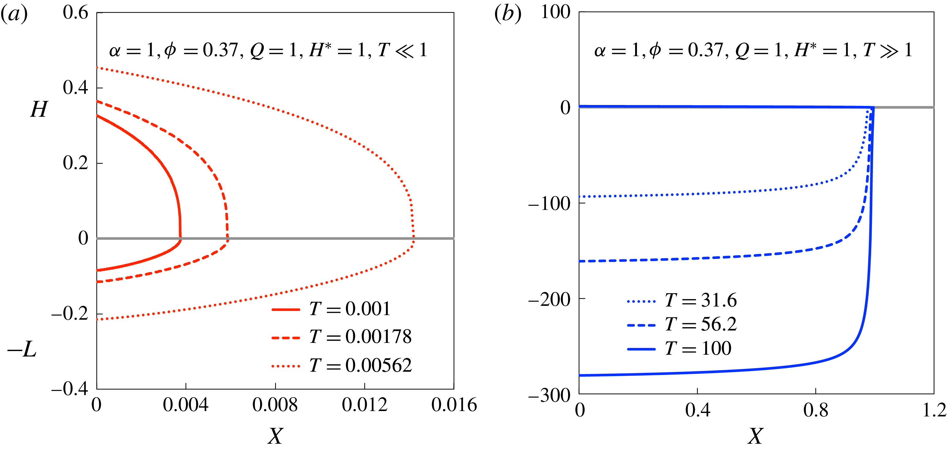
(a) Time evolution of the front location when
 $\unicode[STIX]{x1D6FC}=1$
,
 $\unicode[STIX]{x1D719}=0.37$
and
 $H^{\ast }=1$
. The numerical results of PDEs (3.11a–c
) (black triangles) are compared with the self-similar solutions in the early-time (red dashed curve) and late-time (blue dotted curve) periods. (b) Time evolution of the normalized shape of the current. The numerical results of PDEs (3.11a–c
) at different times
 $T$
are compared with the normalized self-similar solutions in the early-time (thick red line) and late-time (thick blue line) periods. In both cases, the shapes of the current approach the normalized self-similar shapes.

The asymptotic analyses in §§ 3.3.2 and 3.4.2 give the asymptotic solutions for the front location for
 $\unicode[STIX]{x1D6FC}=1$
:
 $$\begin{eqnarray}X_{F}(T)=\left\{\begin{array}{@{}ll@{}}T^{4/5},\quad & T\ll 1,\\ 1,\quad & T\gg 1.\end{array}\right.\end{eqnarray}$$
The front location first advances and finally arrests.
The PDE numerical results of the time evolution of the front location
 $X_{F}(T)$
and the self-similar solutions for
 $\unicode[STIX]{x1D6FC}=1$
in the asymptotic time limits (see (3.59)) are shown in figure 12(a), when
 $\unicode[STIX]{x1D719}=0.37$
and
 $H^{\ast }=1$
. There is good agreement between the PDE solutions (black triangles) and the predictions from the self-similar solutions in both early-time (red dashed curve) and late-time (blue dotted curve) periods. The transition between the early-time and late-time asymptotic behaviours occurs near
 $T=\mathit{O}(1)$
.
Time evolution of the shape of the current under continuous addition when
 $\unicode[STIX]{x1D6FC}=3$
, with
 $\unicode[STIX]{x1D719}=0.37$
,
 $Q=1$
: (a) at early times; (b) at late times. The results are calculated numerically from PDEs (3.11a–c
).

(a) Time evolution of the front location when
 $\unicode[STIX]{x1D6FC}=3$
,
 $\unicode[STIX]{x1D719}=0.37$
and
 $Q\,=1$
. The numerical results of PDEs (3.11a–c
) (black triangles) are compared with the self-similar solutions in early-time (red dashed curve) and late-time (blue dotted curve) periods. (b) Time evolution of the normalized shape of the current, when
 $\unicode[STIX]{x1D6FC}=3$
 $\unicode[STIX]{x1D719}=0.37$
, and
 $Q=1$
. The numerical results of PDEs (3.11a–c
) at different times
 $T$
are compared with the self-similar solutions in early-time (thick red line) and late-time (thick blue line) periods. In both cases, the shapes of the current approach the self-similar shapes in asymptotic limits.

The asymptotic analyses in § 3.3.2 and 3.4.2 also provide the normalized self-similar shapes of the current. For the early-time period, the self-similar depth is given by
 $$\begin{eqnarray}g(s)=2.32~\sqrt{1-s^{5/4}},\quad T\ll 1,\end{eqnarray}$$
while the corresponding self-similar height
 $f(s)$
can be solved numerically. For the late times, the self-similar height
 $f(s)$
and depth
 $g(s)$
are given by (3.47a,b
), respectively. The comparisons of the normalized current shape, i.e.
 $H/H_{max}$
,
 $L/L_{max}$
versus
 $X/X_{F}$
, at different times
 $T$
with the normalized self-similar solutions
 $f/f_{max}$
,
 $g/g_{max}$
versus
 $s$
when
 $\unicode[STIX]{x1D6FC}=1$
,
 $\unicode[STIX]{x1D719}=0.37$
, and
 $H^{\ast }=1$
are shown in figure 12(b). The shapes of the current approach the normalized self-similar shapes in the asymptotic limits,
 $T\ll 1$
or
 $T\gg 1$
.
3.5.3 Continuous addition:
$\unicode[STIX]{x1D6FC}=3$

For continuous addition when
 $\unicode[STIX]{x1D6FC}=3$
, the PDE numerical results of the current shape at different times are shown in figure 13(a) at early times and (b) at late times, with
 $\unicode[STIX]{x1D719}=0.37$
,
 $Q=1$
. The three dimensionless variables,
 $H$
,
 $L$
and
 $X_{F}$
increase during the entire time period. This result is because with a higher addition exponent
 $\unicode[STIX]{x1D6FC}$
, the liquid can still accumulate above the porous medium while draining into the porous medium.
The asymptotic analyses in § 3.3.3 and appendix C provide the early-time and late-time solutions for the front location for
 $\unicode[STIX]{x1D6FC}=3$
. When
 $\unicode[STIX]{x1D719}=0.37$
,
 $Q=1$
, the asymptotic solutions of the front location are
 $$\begin{eqnarray}X_{F}(T)=\left\{\begin{array}{@{}ll@{}}2.37~T^{5/2},\quad & T\ll 1,\\ 0.60~T^{2},\quad & T\gg 1.\end{array}\right.\end{eqnarray}$$
We compare the PDE results of the time evolution of the front location with the asymptotic solutions for
 $\unicode[STIX]{x1D6FC}=3$
,
 $\unicode[STIX]{x1D719}=0.37$
and
 $Q=1$
(see (3.61)) in figure 14(a). There is good agreement between the PDE solutions (black triangles) and the predictions from the asymptotic analysis in both early-time (red dashed line) and late-time (blue dotted line) periods.
In addition, the normalized current shape, i.e.
 $H/H_{max}$
,
 $L/L_{max}$
versus
 $X/X_{F}$
, at different times
 $T$
are compared with the normalized self-similar solutions
 $f/f_{max}$
,
 $g/g_{max}$
versus
 $s$
when
 $\unicode[STIX]{x1D6FC}=3$
,
 $\unicode[STIX]{x1D719}=0.37$
and
 $Q=1$
in figure 14(b). For the early times, the self-similar depth (see § 3.3.3) is given by
 $$\begin{eqnarray}g(s)=2.32~\sqrt{1-s^{2/5}},\quad T\ll 1,\end{eqnarray}$$
while the corresponding self-similar height
 $f(s)$
can be solved numerically. The late-time self-similar shape is solved numerically by the method described in appendix C. In both asymptotic limits, i.e.
 $T\ll 1$
or
 $T\gg 1$
, the normalized current shapes from the numerical results approach the normalized self-similar shapes.
By comparing figures 11(b) and 13(b), we find that as time goes on, for
 $\unicode[STIX]{x1D6FC}=1$
, the current above the porous medium becomes thinner and that in the porous medium becomes fatter, while for
 $\unicode[STIX]{x1D6FC}=3$
, the current above the porous medium stays almost unchanged and that in the porous medium becomes thinner. This difference is because for small
 $\unicode[STIX]{x1D6FC}$
, i.e. a slow addition in the late-time period, spreading of the current is slower than the drainage, which leads to the thinner shape of the liquid above and a fatter shape inside the porous medium, as time goes on. However, for large
 $\unicode[STIX]{x1D6FC}$
, i.e. a rapid addition in the late-time period, spreading of the current is comparable or faster than the drainage, which makes the shape of the current inside the porous medium thinner.
4 The influence of capillary effects
The influence of capillary effects is described by the dimensionless capillary length
 $H^{\ast }$
, as defined in (3.9), which is a measure of the capillary forces relative to the gravitational forces. In the current work, we emphasize the influence of capillary effects by investigating the influence of
 $H^{\ast }$
on both the self-similar solutions of
 $H$
,
 $L$
and
 $X_{F}$
in the asymptotic time limits and the transition between the early-time and the late-time behaviours. We also compare the results with the purely gravity-driven drainage case (Acton et al.
Reference Acton, Huppert and Worster2001), i.e.
 $H^{\ast }=0$
. From the analysis in § 3.4, we know that the capillary forces have no influence on the late-time self-similar solutions. Thus, we focus on the influence of the capillary forces on the early-time self-similar solutions.
4.1 The influence of capillary effects on the early-time self-similar solutions
Based on the analysis in § 3.3, we know the time dependence of the variables in the early-time period, i.e.
 $H\propto T^{A}$
,
 $L\propto T^{B}$
,
 $X_{F}\propto T^{C}$
, where the time exponents
 $A$
,
 $B$
and
 $C$
are given as the scaling exponents in table 1. Thus, we can write the dimensionless variables as
 $$\begin{eqnarray}H(X,T)=T^{A}M_{H}\frac{f(s)}{f_{max}},\quad L(X,T)=T^{B}M_{L}\frac{g(s)}{g_{max}},\quad \text{and}\quad X_{F}(T)=T^{C}M_{X},\end{eqnarray}$$
where
 $M_{H}$
,
 $M_{L}$
and
 $M_{X}$
are the magnitudes of the height
 $H$
, the length
 $L$
and the front location
 $X_{F}$
. For
 $\unicode[STIX]{x1D6FC}\neq 3$
, they are defined as
 $$\begin{eqnarray}M_{H}\equiv (H^{\ast })^{a}\unicode[STIX]{x1D719}^{\unicode[STIX]{x1D711}}\unicode[STIX]{x1D709}_{f}^{m}f_{max},\quad M_{L}\equiv (H^{\ast })^{b}\unicode[STIX]{x1D719}^{\unicode[STIX]{x1D712}}\unicode[STIX]{x1D709}_{f}^{n}g_{max},\quad \text{and}\quad M_{X}\equiv (H^{\ast })^{c}\unicode[STIX]{x1D719}^{\unicode[STIX]{x1D713}}\unicode[STIX]{x1D709}_{f}.\end{eqnarray}$$
The values of the exponents
 $a$
,
 $b$
,
 $c$
,
 $m$
,
 $n$
,
 $\unicode[STIX]{x1D711}$
,
 $\unicode[STIX]{x1D712}$
and
 $\unicode[STIX]{x1D713}$
for different
 $\unicode[STIX]{x1D6FC}$
are given in § 3.3 and appendix B. For
 $\unicode[STIX]{x1D6FC}=3$
,
 $M_{H}$
,
 $M_{L}$
and
 $M_{X}$
(see § 3.3.3) depend on
 $Q$
instead of
 $H^{\ast }$
, and are given by
 $$\begin{eqnarray}M_{H}\equiv Q^{1/2}\unicode[STIX]{x1D719}^{-1/8}\unicode[STIX]{x1D709}_{f}^{1/2}f_{max},\quad M_{L}\equiv \unicode[STIX]{x1D719}^{-1/2}g_{max},\quad \text{and}\quad M_{X}\equiv Q\unicode[STIX]{x1D719}^{-1/2}\unicode[STIX]{x1D709}_{f}.\end{eqnarray}$$
Based on (4.1a–c
), the influence of capillary effects on the early-time self-similar solutions are divided into three parts: (i) the capillary effects influence the time dependence, i.e.
 $H^{\ast }$
influences the values of
 $A$
,
 $B$
and
 $C$
. (ii) The capillary effects influence the magnitudes of the asymptotic solutions, i.e.
 $H^{\ast }$
influences
 $M_{H}$
,
 $M_{L}$
and
 $M_{X}$
. (iii) The capillary effects influence the normalized self-similar shapes of the current, i.e.
 $H^{\ast }$
influences
 $f(s)/f_{max}$
and
 $g(s)/g_{max}$
. We summarize the influence of the capillary effects, i.e.
 $H^{\ast }$
, on the asymptotic solutions of
 $H$
,
 $L$
and
 $X_{F}$
in the early-time period for different addition exponents
 $\unicode[STIX]{x1D6FC}$
in table 3.
The influence of capillary forces on the magnitudes of the early-time asymptotic solutions when
 $\unicode[STIX]{x1D719}=0.37$
. (a) The magnitude of the depth
 $M_{L}$
as a function of the dimensionless capillary length
 $H^{\ast }$
, when
 $\unicode[STIX]{x1D6FC}=1/2,7/4$
. (b) The magnitudes of the height and the front location, i.e.
 $M_{H}$
and
 $M_{X}$
, as functions of
 $H^{\ast }$
when
 $\unicode[STIX]{x1D6FC}=7/4$
.

The influence of capillary effects, i.e.
 $H^{\ast }$
, on the asymptotic solutions of
 $H$
,
 $L$
and
 $X_{F}$
in the early-time period (
 $T\ll 1$
) for different addition exponents
 $\unicode[STIX]{x1D6FC}$
. In the late-time period (
 $T\gg 1$
),
 $H^{\ast }$
has no effects on the asymptotic behaviours.

For the influence of the capillary forces on the time dependence, we find that when
 $H^{\ast }>0$
, the time exponents
 $A$
,
 $B$
and
 $C$
(see table 1) depend only on
 $\unicode[STIX]{x1D6FC}$
but not
 $H^{\ast }$
. For the limiting case when
 $H^{\ast }=0$
, i.e. the purely gravity-driven drainage, the time dependence is also listed in table 3. By comparing the time dependence of capillarity and gravity-driven drainage (
 $H^{\ast }>0$
) with that of purely gravity-driven drainage (
 $H^{\ast }=0$
), we find that for
 $\unicode[STIX]{x1D6FC}<1/2$
, there is no influence of capillary effects on the time dependence. For
 $1/2\leqslant \unicode[STIX]{x1D6FC}\leqslant 7/4$
, capillary effects enhance the accumulation of the liquid in the porous medium, which can be seen from the smaller time exponent
 $B$
for
 $H^{\ast }>0$
compared with
 $H^{\ast }=0$
. For
 $\unicode[STIX]{x1D6FC}>7/4$
, capillary effects not only enhance the accumulation of the liquid in the porous medium, but also hinder the accumulation and spreading of the liquid above the porous medium, i.e. greater
 $A$
and
 $C$
for
 $H^{\ast }>0$
compared with
 $H^{\ast }=0$
.
Capillary effects influence the magnitudes in two ways: first, when
 $1/2<\unicode[STIX]{x1D6FC}<7/4$
or
 $\unicode[STIX]{x1D6FC}>7/4$
,
 $M_{H}$
,
 $M_{L}$
and
 $M_{X}$
simply scale with
 $H^{\ast }$
, i.e.
 $a$
,
 $b$
,
 $c$
are not all zero and the governing equations for
 $f(s)$
,
 $g(s)$
and
 $\unicode[STIX]{x1D709}_{f}$
are independent of
 $H^{\ast }$
(see §§ 3.3.2 and 3.3.3). Second, when
 $\unicode[STIX]{x1D6FC}=1/2$
or
 $7/4$
, there is no scaling relationship, i.e.
 $a=b=c=0$
and the governing equations for
 $f(s)$
,
 $g(s)$
and
 $\unicode[STIX]{x1D709}_{f}$
includes
 $H^{\ast }$
(see appendices B.1 and B.2). For the second case, the dependence of the magnitudes on the capillary effects is shown in figure 15(a) for the dependence of
 $M_{L}$
on
 $H^{\ast }$
for both
 $\unicode[STIX]{x1D6FC}=1/2$
and
 $7/4$
, and in figure 15(b) for the dependence of
 $M_{H}$
and
 $M_{X}$
on
 $H^{\ast }$
for
 $\unicode[STIX]{x1D6FC}=7/4$
. From figure 15(a), we find that when
 $\unicode[STIX]{x1D6FC}=1/2$
and
 $7/4$
,
 $M_{L}$
increases with
 $H^{\ast }$
, and there is an asymptotic relation
 $M_{L}\propto (H^{\ast })^{1/2}$
for large
 $H^{\ast }$
. From figure 15(b), it can be seen that for
 $\unicode[STIX]{x1D6FC}=7/4$
, both
 $M_{H}$
and
 $M_{X}$
decrease when
 $H^{\ast }$
increases.
To summarize, for
 $\unicode[STIX]{x1D6FC}<1/2$
, there is no influence of
 $H^{\ast }$
on the magnitudes
 $M_{H}$
,
 $M_{L}$
and
 $M_{X}$
. For
 $1/2\leqslant \unicode[STIX]{x1D6FC}<7/4$
,
 $M_{L}$
increases with
 $H^{\ast }$
, while
 $M_{H}$
and
 $M_{X}$
are independent of
 $H^{\ast }$
. Finally, for
 $\unicode[STIX]{x1D6FC}\geqslant 7/4$
and
 $\unicode[STIX]{x1D6FC}\neq 3$
,
 $M_{L}$
increases, while
 $M_{H}$
and
 $M_{X}$
decrease when
 $H^{\ast }$
increases.
The capillary effects influence the normalized self-similar shapes only when
 $\unicode[STIX]{x1D6FC}=1/2$
and
 $7/4$
. As shown in figure 16, greater capillary forces, i.e. larger
 $H^{\ast }$
, correspond to a fatter shape of
 $g(s)/g_{max}$
for both
 $\unicode[STIX]{x1D6FC}=1/2$
, and a thinner shape of
 $f(s)/f_{max}$
for
 $\unicode[STIX]{x1D6FC}=7/4$
.
The influence of capillary forces on the normalized early-time self-similar shape of the current when
 $\unicode[STIX]{x1D719}=0.37$
and (a)
 $\unicode[STIX]{x1D6FC}=1/2$
, (b)
 $\unicode[STIX]{x1D6FC}=7/4$
. The normalized early-time self-similar shapes of a purely gravity-driven current, i.e.
 $H^{\ast }=0$
are also shown in both cases.

4.2 The influence of capillary effects on the transition between early-time and late-time behaviours
In order to study the influence of capillary effects on the transition between the early-time and the late-time behaviours, we focus on the case when
 $\unicode[STIX]{x1D6FC}=1$
, where the value of
 $H^{\ast }$
does not influence the self-similar solutions of the front location
 $X_{F}(T)$
in both the early-time and late-time periods. As shown in figure 17, the PDE numerical solutions of the front location
 $X_{F}(T)$
for
 $H^{\ast }=100$
depart earlier from the early-time self-similar solution and approach later to the late-time self-similar solution than the PDE numerical solutions for
 $H^{\ast }=1$
. The results indicate that greater capillary effects elongate the transition period between the early-time and late-time asymptotic behaviours.
The time evolution of the front location
 $X_{F}(T)$
under different dimensionless capillary lengths
 $H^{\ast }=1,100$
, when
 $\unicode[STIX]{x1D6FC}=1$
,
 $\unicode[STIX]{x1D719}=0.37$
. The PDE solutions show that greater capillary effects, i.e. larger
 $H^{\ast }$
, result in an earlier departure of the front location
 $X_{F}(T)$
from the early-time self-similar solution while later they approach the late-time self-similar solution.

5 Summary and conclusions
In this paper, we theoretically and numerically studied the influence of capillary effects on the drainage of a viscous gravity current into an infinitely deep porous medium, which is wettable by the liquid. First, we investigated the one-dimensional problem driven by both the gravitational and capillary forces in § 2. Depending on the value of the addition exponent,
 $\unicode[STIX]{x1D6FC}$
, there are three drain-out scenarios. In addition, we found that the influence of the capillary effects is limited to the early-time period, where it enhances the drainage.
Secondly, we addressed the two-dimensional problem in § 3, where the viscous gravity current drains into the porous medium while spreading above it. Since there are no self-similar solutions for the front location and the current shape for the entire time period, asymptotic analysis is employed to solve for self-similar solutions in both the early-time and late-time periods. Different solutions are found depending on the value of the addition exponent
 $\unicode[STIX]{x1D6FC}$
. We also numerically solved the partial differential equations to show the transition between the early-time and late-time asymptotic behaviours. The PDE solutions show good agreement with the self-similar solutions in asymptotic time limits. In addition, we discussed the influence of the capillary effects on both the asymptotic behaviours and the transition between them. For the former case, the results show that the capillary effects have no influence on the late-time asymptotic behaviours, and the influence of the capillary effects on the early-time asymptotic behaviours varies with
 $\unicode[STIX]{x1D6FC}$
as summarized in § 4. For the latter case, it is shown that the capillary effects elongate the transition period between the early-time and late-time asymptotic behaviours.
The current work highlights that the capillary effects can increase the early-time leakage of the liquid into a deep porous medium that is wettable by the liquid. For example, the leakage of a saline water current into a permeable bottom of an estuary depends on the pore sizes or wettability of the porous medium. Furthermore, one natural extension of the current work is to a gravity current spreading within a porous medium while it also drains into a permeable substrate. For example, this problem is closely related to industrial projects of geological
 $\text{CO}_{2}$
sequestration and the leakage of supercritical
 $\text{CO}_{2}$
from a underground storage sites (see, e.g. Lyle et al.
Reference Lyle, Huppert, Hallworth, Bickle and Chadwick2005; Woods & Farcas Reference Woods and Farcas2009; Huppert & Neufeld Reference Huppert and Neufeld2014; Zheng et al.
Reference Zheng, Guo, Christov, Celia and Stone2015a
; Guo et al.
Reference Guo, Zheng, Celia and Stone2016). The current work shows how to study the capillary effects on the liquid drainage into a permeable substrate, which can enhance the
 $\text{CO}_{2}$
leakage from the geological sequestration projects when
 $\text{CO}_{2}$
wets the porous substrates.
We note that our model does not consider the hydrodynamic instability at the fluid–fluid interface when a heavier fluid spreads above a lighter fluid. This gravitational instability is observed experimentally in the late-time period during the spreading of a gravity current over a porous medium, for example, by Acton et al. (Reference Acton, Huppert and Worster2001). However, the new flow regimes we identified in this paper only exist in the early-time period, when the capillary effects are important. In the late-time period, our model recovers that of pure gravity-driven drainage (Acton et al. Reference Acton, Huppert and Worster2001), and the effects of gravitational instability are likely to be important as time progresses. The detailed study is left for future work.
Acknowledgement
We thank the Carbon Mitigation Initiative of Princeton University (sponsored by BP) for support of this research.
Appendix A. Method to determine regimes
Here we describe the method we use to determine regimes according to the values of the addition exponent
 $\unicode[STIX]{x1D6FC}$
in the early-time and late-time asymptotic behaviours (see tables 1, 2). Generally speaking, we compare the magnitudes for different terms in (3.11a–c
). For convenience, we sum up (3.11a
) and (3.11b
), which yields
 $$\begin{eqnarray}\frac{\unicode[STIX]{x2202}H}{\unicode[STIX]{x2202}T}-\frac{\unicode[STIX]{x2202}}{\unicode[STIX]{x2202}X}\left(H^{3}\frac{\unicode[STIX]{x2202}H}{\unicode[STIX]{x2202}X}\right)+\unicode[STIX]{x1D719}\frac{\unicode[STIX]{x2202}L}{\unicode[STIX]{x2202}T}=0.\end{eqnarray}$$
A.1 Determining early-time regimes
We know that
 $L$
increases with
 $T$
from (3.11b
), so in the early-time period, i.e.
 $T\ll 1$
, we have
 $L\ll 1$
. Meanwhile, we know that the liquid supply rate
 $Q_{supp}=\unicode[STIX]{x1D6FC}T^{\unicode[STIX]{x1D6FC}-1}$
increases with decreasing
 $\unicode[STIX]{x1D6FC}$
, and in the limit when
 $\unicode[STIX]{x1D6FC}\rightarrow 0$
,
 $H\rightarrow H_{0}>0$
. Thus,
 $H$
is larger for smaller
 $\unicode[STIX]{x1D6FC}$
.
Therefore, from (A 1) and (3.11b,c
), we can find three regimes. (i) When
 $\unicode[STIX]{x1D6FC}$
is small,
 $H\gg L$
and
 $H\gg H^{\ast }$
, thus we balance the first two terms of (A 1), i.e.
 $H/T\sim H^{4}/X^{2}$
, the left-hand side with the first term on the right-hand side in (3.11b
), i.e.
 $L/T\sim H/L$
, and the first term on the left-hand side with the right-hand side of (3.11c
), i.e.
 $HX\sim T^{\unicode[STIX]{x1D6FC}}$
. (ii) For moderate
 $\unicode[STIX]{x1D6FC}$
,
 $H\gg L$
but
 $H\ll H^{\ast }$
, the only difference with the first regime is that we balance the left-hand side with the first term on the right-hand side of (3.11b
), i.e.
 $L/T\sim H^{\ast }/L$
. (iii) For large
 $\unicode[STIX]{x1D6FC}$
,
 $H\ll L$
and
 $H\ll H^{\ast }$
, we balance the last two terms of (A 1), i.e.
 $H^{4}/X^{2}\sim L/T$
, the left-hand side with the second term on the right-hand side of (3.11b
), i.e.
 $L/T\sim H^{\ast }/L$
, and the second term on the left-hand side with the right-hand side of (3.11c
), i.e.
 $LX\sim T^{\unicode[STIX]{x1D6FC}}$
. We can determine the boundary between regime I and II by setting
 $H/T\sim H^{4}/X^{2}$
,
 $L/T\sim /L\sim H^{\ast }/L$
and
 $HX\sim T^{\unicode[STIX]{x1D6FC}}$
, which yields
 $\unicode[STIX]{x1D6FC}=1/2$
. The boundary between regime II and III is found by setting
 $H/T\sim H^{4}/X^{2}\sim H^{\ast }/L$
,
 $L/T\sim H^{\ast }/L$
and
 $HX\sim LX\sim T^{\unicode[STIX]{x1D6FC}}$
, which yields
 $\unicode[STIX]{x1D6FC}=7/4$
.
A.2 Determining late-time regimes
In the late-time period, i.e.
 $T\gg 1$
, the liquid supply rate
 $Q_{supp}=\unicode[STIX]{x1D6FC}T^{\unicode[STIX]{x1D6FC}-1}$
increases with increasing
 $\unicode[STIX]{x1D6FC}$
. Thus,
 $H$
is larger for larger
 $\unicode[STIX]{x1D6FC}$
. Also, because
 $L$
increases with
 $T$
, we have
 $L\gg 1$
in the late-time period.
Therefore, from (A 1) and (3.17b,c
), we can find two regimes. (i) For small
 $\unicode[STIX]{x1D6FC}$
,
 $H\ll L$
, we balance the second term on the left-hand side with the last term on the right-hand side of (3.11a
), i.e.
 $H^{4}/X^{2}\sim 1$
, the left-hand side with the last term on the right-hand side of (3.11b
), i.e.
 $L/T\sim 1$
, and the second term on the left-hand side with the right-hand side of (3.11c
), i.e.
 $LX\sim T^{\unicode[STIX]{x1D6FC}}$
. (ii) For large
 $\unicode[STIX]{x1D6FC}$
,
 $H\ll L$
, we balance the first term with the second term on the left-hand side of (3.11a
), i.e.
 $H/T\sim H^{4}/X^{2}$
, the left-hand side with the first term on the right-hand side of (3.11b
), i.e.
 $L/T\sim H/L$
, and the first term on the left-hand side with the right-hand side of (3.11c
), i.e.
 $HX\sim T^{\unicode[STIX]{x1D6FC}}$
. The regime boundary is found by setting
 $H/T\sim H^{4}/X^{2}\sim 1$
,
 $L/T\sim H/L\sim 1$
and
 $HX\sim LX\sim T^{\unicode[STIX]{x1D6FC}}$
, which yields
 $\unicode[STIX]{x1D6FC}=3$
.
Appendix B. The early-time self-similar solutions
B.1 The special case:
$\unicode[STIX]{x1D6FC}=1/2$

In the early-time period, i.e.
 $T\ll 1$
, for
 $\unicode[STIX]{x1D6FC}=1/2$
, the governing equations (3.11a–c
) reduce to
 $$\begin{eqnarray}\displaystyle & \displaystyle \frac{\unicode[STIX]{x2202}H}{\unicode[STIX]{x2202}T}-\frac{\unicode[STIX]{x2202}}{\unicode[STIX]{x2202}X}\left(H^{3}\frac{\unicode[STIX]{x2202}H}{\unicode[STIX]{x2202}X}\right)=0, & \displaystyle\end{eqnarray}$$
 $$\begin{eqnarray}\displaystyle & \displaystyle \frac{\unicode[STIX]{x2202}L}{\unicode[STIX]{x2202}T}=\frac{1}{\unicode[STIX]{x1D719}}\frac{H+H^{\ast }}{L}, & \displaystyle\end{eqnarray}$$
 $$\begin{eqnarray}\displaystyle & \displaystyle \int _{0}^{X_{F}(T)}H(X,T)\,\text{d}X=T^{1/2}. & \displaystyle\end{eqnarray}$$
The solutions for
 $H(X,T)$
and
 $X_{F}(T)$
should be the same as those in regime I (see § 3.3.1) because the relevant governing equations (B 1a,c
) are the same as (3.17a,c
) and they are subject to the same boundary and initial conditions. In other words, we can define
 $X_{F}=\unicode[STIX]{x1D709}_{f}T^{1/2}$
,
 $H=\unicode[STIX]{x1D709}_{f}^{2/3}f(s)$
, and
 $s\equiv X/(\unicode[STIX]{x1D709}_{f}T^{1/2})$
, where
 $f(s)$
and
 $\unicode[STIX]{x1D709}_{f}$
are the same as that in regime I. Thus, we find
 $\unicode[STIX]{x1D709}_{f}\approx 1.112$
for
 $\unicode[STIX]{x1D6FC}=1/2$
.
In addition, we can write
 $L$
in a self-similar form as
 $L=\unicode[STIX]{x1D719}^{-1/2}\unicode[STIX]{x1D709}_{f}^{1/3}T^{1/2}g(s)$
. Given the solution of
 $f(s)$
, then
 $g(s)$
can be determined numerically from
 $$\begin{eqnarray}sg^{\prime }-g+2\frac{f}{g}+2\unicode[STIX]{x1D709}_{f}^{-2/3}\frac{H^{\ast }}{g}=0,\end{eqnarray}$$
subject to the boundary condition
 $g(1)=0$
.
It can be seen from (B 2) that the value of
 $H^{\ast }$
influences the solution for
 $g(s)$
and also the normalized depth
 $g(s)/g_{max}$
. As an example, the normalized self-similar shape for
 $\unicode[STIX]{x1D6FC}=1/2$
and
 $H^{\ast }=1$
is shown in figure 4 as the blue curve.
Remembering that the current theory is based on the assumptions that
 $x_{f}(t)\gg h(0,t)$
,
 $x_{f}(t)\gg \ell (0,t)$
and
 $|\text{d}x_{f}/\text{d}t|\gg |\unicode[STIX]{x2202}\ell /\unicode[STIX]{x2202}t|$
, we can obtain the self-consistent requirements:
 $$\begin{eqnarray}T\gg \left(\frac{gk^{5/2}}{q^{2}\unicode[STIX]{x1D708}}\right)^{2/5},\quad \text{and}\quad \unicode[STIX]{x1D719}^{-1/2}\left(\frac{gk^{5/2}}{q^{2}\unicode[STIX]{x1D708}}\right)^{1/5}.\end{eqnarray}$$
As long as the right-hand side of (B 3a
) is much smaller than
 $1$
and (B 3b
) is satisfied, the drainage theory is valid in the early-time period.
B.2 The special case:
$\unicode[STIX]{x1D6FC}=7/4$

In the early-time period, i.e.
 $T\ll 1$
, for
 $\unicode[STIX]{x1D6FC}=7/4$
the governing equations (3.11a–c
) reduce to
 $$\begin{eqnarray}\displaystyle & \displaystyle \frac{\unicode[STIX]{x2202}H}{\unicode[STIX]{x2202}T}-\frac{\unicode[STIX]{x2202}}{\unicode[STIX]{x2202}X}\left(H^{3}\frac{\unicode[STIX]{x2202}H}{\unicode[STIX]{x2202}X}\right)=-\frac{H^{\ast }}{L}, & \displaystyle\end{eqnarray}$$
 $$\begin{eqnarray}\displaystyle & \displaystyle \frac{\unicode[STIX]{x2202}L}{\unicode[STIX]{x2202}T}=\frac{1}{\unicode[STIX]{x1D719}}\frac{H^{\ast }}{L}, & \displaystyle\end{eqnarray}$$
 $$\begin{eqnarray}\displaystyle & \displaystyle \int _{0}^{X_{F}(T)}\left(H+\unicode[STIX]{x1D719}L\right)\,\text{d}X=\frac{1}{\unicode[STIX]{x1D719}}T^{7/4}. & \displaystyle\end{eqnarray}$$
A self-similar variable is defined as
 $s\equiv X/(\unicode[STIX]{x1D709}_{f}T^{5/4})$
, and we can rewrite the functions as
 $X_{F}=\unicode[STIX]{x1D709}_{f}T^{5/4}$
,
 $H=\unicode[STIX]{x1D709}_{f}^{2/3}T^{1/2}f(s)$
and
 $L=(H^{\ast }/\unicode[STIX]{x1D719})^{1/2}T^{1/2}g(s)$
on the domain
 $s\in [0,1]$
. In this way, we can rewrite the (B 4a–c
) as
 $$\begin{eqnarray}\displaystyle & \displaystyle (f^{3}f^{\prime })^{\prime }+\frac{5}{4}sf^{\prime }-\frac{1}{2}f-\unicode[STIX]{x1D709}_{f}^{-2/3}\frac{\left(H^{\ast }\unicode[STIX]{x1D719}\right)^{1/2}}{g}=0, & \displaystyle\end{eqnarray}$$
 $$\begin{eqnarray}\displaystyle & \displaystyle \frac{5}{4}sg^{\prime }-\frac{1}{2}g+\frac{1}{\unicode[STIX]{x1D719}}\frac{H^{\ast }}{g}=0, & \displaystyle\end{eqnarray}$$
 $$\begin{eqnarray}\displaystyle & \displaystyle \unicode[STIX]{x1D709}_{f}^{5/3}\int _{0}^{1}f(s)\,\text{d}s+\unicode[STIX]{x1D709}_{f}\left(H^{\ast }\unicode[STIX]{x1D719}\right)^{1/2}\int _{0}^{1}g(s)\,\text{d}s-1=0. & \displaystyle\end{eqnarray}$$
The solution of
 $g(s)$
should be the same as those in regimes II and III (see § 3.3.2, 3.3.3), because the governing equation (B 5b
) is the same as equations (3.24b
) and (3.31b
) when setting
 $\unicode[STIX]{x1D6FC}=7/4$
, and also the boundary condition
 $g(1)=0$
. Thus, we can obtain
 $$\begin{eqnarray}g(s)=\left[2\left(1-s^{4/5}\right)\right]^{1/2}.\end{eqnarray}$$
The local asymptotic analysis of (B 5a
) near
 $s=1$
yields
 $$\begin{eqnarray}f(s)\sim \left(\frac{15}{4}\right)^{1/3}(1-s)^{1/3}\quad \text{as}~s\rightarrow 1^{-},\end{eqnarray}$$
which provides the values of
 $f(1-\unicode[STIX]{x1D716})$
and
 $f^{\prime }(1-\unicode[STIX]{x1D716})$
for
 $\unicode[STIX]{x1D716}\ll 1$
. These conditions can be used to numerically solve ODEs (B 5a,c
) by shooting from
 $s=1-\unicode[STIX]{x1D716}$
towards
 $s=0$
for a given
 $\unicode[STIX]{x1D709}_{f}$
. We search for
 $\unicode[STIX]{x1D709}_{f}$
until the value of the left-hand side of (B 5c
) is smaller than
 $10^{-6}$
.
It can be seen from (B 5a,c
) that the values of both
 $H^{\ast }$
and
 $\unicode[STIX]{x1D719}$
influence the solutions for
 $f(s)$
and
 $\unicode[STIX]{x1D709}_{f}$
, and also the normalized height
 $f(s)/f_{max}$
. As an example, the normalized self-similar shape for
 $\unicode[STIX]{x1D6FC}=7/4$
,
 $\unicode[STIX]{x1D719}=0.37$
and
 $H^{\ast }=1$
is shown in figure 4 as the orange curve. The stretching constant is computed as
 $\unicode[STIX]{x1D709}_{f}\approx 0.65$
.
The assumptions that
 $x_{f}(t)\gg h(0,t)$
,
 $x_{f}(t)\gg \ell (0,t)$
and
 $|\text{d}x_{f}/\text{d}t|\gg |\unicode[STIX]{x2202}\ell /\unicode[STIX]{x2202}t|$
provide the self-consistent requirements:
 $$\begin{eqnarray}T\gg \left(\frac{g^{7/2}k^{15/4}}{q^{2}\unicode[STIX]{x1D708}^{7/2}}\right)^{8/15}\quad \text{and}\quad T\gg \left(\frac{H^{\ast }}{\unicode[STIX]{x1D719}}\right)^{2/3}\left(\frac{g^{7/2}k^{15/4}}{q^{2}\unicode[STIX]{x1D708}^{7/2}}\right)^{8/15}.\end{eqnarray}$$
As long as the right-hand sides of (B 8a,b
) are much smaller than
 $1$
, the drainage theory is valid in a broad portion of the early-time period.
Appendix C. The late-time self-similar solutions when
$\unicode[STIX]{x1D6FC}=3$

In the late-time period, i.e.
 $T\gg 1$
, for
 $\unicode[STIX]{x1D6FC}=3$
the governing equations (3.13a–c
) reduce to
 $$\begin{eqnarray}\displaystyle & \displaystyle \frac{\unicode[STIX]{x2202}H}{\unicode[STIX]{x2202}T}-\frac{\unicode[STIX]{x2202}}{\unicode[STIX]{x2202}X}\left(H^{3}\frac{\unicode[STIX]{x2202}H}{\unicode[STIX]{x2202}X}\right)=-1, & \displaystyle\end{eqnarray}$$
 $$\begin{eqnarray}\displaystyle & \displaystyle \frac{\unicode[STIX]{x2202}L}{\unicode[STIX]{x2202}T}=\frac{1}{\unicode[STIX]{x1D719}}\left(\frac{H}{L}+1\right), & \displaystyle\end{eqnarray}$$
 $$\begin{eqnarray}\displaystyle & \displaystyle \int _{0}^{X_{F}(T)}(H+\unicode[STIX]{x1D719}L)\,\text{d}X=QT^{3}. & \displaystyle\end{eqnarray}$$
By defining the similarity variable
 $s\equiv X/(\unicode[STIX]{x1D709}_{f}T^{2})$
, we can rewrite the functions as
 $X_{F}=\unicode[STIX]{x1D709}_{f}T^{2}$
,
 $H=\unicode[STIX]{x1D709}_{f}^{2/3}Tf(s)$
and
 $L=\unicode[STIX]{x1D709}_{f}^{1/3}Tg(s)$
on the domain
 $s\in [0,1]$
, and then write equations (C 1a–c
) as
 $$\begin{eqnarray}\displaystyle & \displaystyle (f^{3}f^{\prime })^{\prime }+2sf^{\prime }-f-\unicode[STIX]{x1D709}_{f}^{-2/3}=0, & \displaystyle\end{eqnarray}$$
 $$\begin{eqnarray}\displaystyle & \displaystyle 2sg^{\prime }-g+\frac{1}{\unicode[STIX]{x1D719}}\frac{f}{g}+\frac{\unicode[STIX]{x1D709}_{f}^{-1/3}}{\unicode[STIX]{x1D719}}=0, & \displaystyle\end{eqnarray}$$
 $$\begin{eqnarray}\displaystyle & \displaystyle \unicode[STIX]{x1D709}_{f}^{5/3}\int _{0}^{1}f(s)\,\text{d}s+\unicode[STIX]{x1D709}_{f}^{4/3}\unicode[STIX]{x1D719}\int _{0}^{1}g(s)\,\text{d}s-Q=0, & \displaystyle\end{eqnarray}$$
 $f(1)=g(1)=0$
.
The local analysis of (C 2a
) near
 $s=1$
yields
 $$\begin{eqnarray}f(s)\sim 6^{1/3}(1-s)^{1/3}\quad \text{as}~s\rightarrow 1^{-}.\end{eqnarray}$$
Equation (C 3) provides the values of
 $f(1-\unicode[STIX]{x1D716})$
and
 $f^{\prime }(1-\unicode[STIX]{x1D716})$
for
 $\unicode[STIX]{x1D716}\ll 1$
. Together with
 $g(1)=0$
, they can be used to numerically solve ODEs (C 2a,b
) by shooting from
 $s=1-\unicode[STIX]{x1D716}$
towards
 $s=0$
for a given
 $\unicode[STIX]{x1D709}_{f}$
. We search for
 $\unicode[STIX]{x1D709}_{f}$
until the value of the left-hand side of (C 2c
) is smaller than
 $10^{-6}$
. From (C 3), we can see that the values of both
 $Q$
and
 $\unicode[STIX]{x1D719}$
influence the solutions for
 $f(s)$
,
 $g(s)$
and
 $\unicode[STIX]{x1D709}_{f}$
, and also the normalized current shape
 $f(s)/f_{max}$
and
 $g(s)/g_{max}$
. As an example, the normalized self-similar shape for
 $\unicode[STIX]{x1D6FC}=3$
,
 $\unicode[STIX]{x1D719}=0.37$
and
 $Q=1$
is shown in figure 6 as the green curve with the stretching constant
 $\unicode[STIX]{x1D709}_{f}\approx 0.60$
.
The assumptions that
 $x_{f}(t)\gg h(0,t)$
,
 $x_{f}(t)\gg \ell (0,t)$
and
 $|\text{d}x_{f}/\text{d}t|\gg |\unicode[STIX]{x2202}\ell /\unicode[STIX]{x2202}t|$
provide the self-consistent requirement:
 $$\begin{eqnarray}T\gg \frac{k^{1/2}R\unicode[STIX]{x1D70C}g}{\unicode[STIX]{x1D6FE}\text{cos}\unicode[STIX]{x1D703}}.\end{eqnarray}$$
As long as the right-hand side of (C 4) is of order
 $1$
or much smaller than
 $1$
, the drainage theory is valid in the late-time period.
Appendix D. The influence of addition rate for
$\unicode[STIX]{x1D6FC}=3$

Now, we discuss the influence of addition rate,
 $Q$
, on the dynamics of the current for
 $\unicode[STIX]{x1D6FC}=3$
. Here, we focus on the effects of
 $Q$
on the early-time self-similar and late-time self-similar solutions.
The influence of addition rate
 $Q$
on the late-time asymptotic solutions when
 $\unicode[STIX]{x1D6FC}=3,\unicode[STIX]{x1D719}=0.37$
. (a) The influence of
 $Q$
on the magnitudes of the height
 $M_{H}$
, the depth
 $M_{L}$
and the front location
 $M_{X}$
. (b) The influence of
 $Q$
on the late-time normalized self-similar shapes.

For the early-time self-similar solutions,
 $Q$
does not influence the normalized self-similar solutions
 $f(s)/f_{max}$
and
 $g(s)/g_{max}$
, but influences the magnitudes
 $M_{H}$
and
 $M_{X}$
, which are defined in (4.3a,c
). There is simple scaling dependence,
 $M_{H}\propto Q^{1/2}$
and
 $M_{X}\propto Q$
.
For the late-time self-similar solutions, the three magnitudes are given by
 $$\begin{eqnarray}M_{H}\equiv \unicode[STIX]{x1D709}_{f}^{2/3}f_{max},\quad M_{L}\equiv \unicode[STIX]{x1D709}_{f}^{1/3}g_{max},\quad \text{and}\quad M_{X}\equiv \unicode[STIX]{x1D709}_{f}.\end{eqnarray}$$
Since the solutions for
 $f(s)$
,
 $g(s)$
and
 $\unicode[STIX]{x1D709}_{f}$
depend on
 $Q$
(see (C 2a–c
)), both the magnitudes
 $M_{H}$
,
 $M_{L}$
and
 $M_{X}$
in (D 1a–c
), and the normalized self-similar solutions
 $f(s)/f_{max}$
and
 $g(s)/g_{max}$
should also depend on
 $Q$
. As an example, we show the dependence of the three magnitudes on
 $Q$
when
 $\unicode[STIX]{x1D719}=0.37$
in figure 18(a), and the normalized self-similar shape under different
 $Q$
in figure 18(b). The result indicates that in the late times, i.e.
 $T\gg 1$
, the magnitudes are higher and the normalized current shape is fatter for higher injection rate
 $Q$
, i.e.
 $H(X,T)$
,
 $L(X,T)$
and
 $X_{F}(T)$
all increase with
 $Q$
.
Appendix E. Numerical scheme
In this section, we describe a cell-centred finite-difference numerical method capable of handling the coupled PDEs (3.11a–c
) for
 $\unicode[STIX]{x1D6FC}\neq 3$
in § 3 and (C 1a–c
) for
 $\unicode[STIX]{x1D6FC}=3$
with boundary conditions given by (3.14a,b
) and initial conditions given by either equations (3.7) or (3.8). We use
 $$\begin{eqnarray}J(X,T)=H^{3}\frac{\unicode[STIX]{x2202}H}{\unicode[STIX]{x2202}X}\end{eqnarray}$$
to represent the flux. The global volume conservation equation (3.11c
) is equivalent to a boundary condition at
 $X=0$
,
 $$\begin{eqnarray}J(0,T)=\left\{\begin{array}{@{}ll@{}}-\unicode[STIX]{x1D6FC}T^{\unicode[STIX]{x1D6FC}-1},\quad & \unicode[STIX]{x1D6FC}>0,\\ 0,\quad \quad & \unicode[STIX]{x1D6FC}=0.\end{array}\right.\end{eqnarray}$$
In order to avoid the singularity on the right-hand sides of (3.11a,b
) for small
 $L$
, we define new variables
 $$\begin{eqnarray}\displaystyle & \displaystyle \unicode[STIX]{x1D6F4}(X,T)\equiv H(X,T)+\unicode[STIX]{x1D719}L(X,T), & \displaystyle\end{eqnarray}$$
 $$\begin{eqnarray}\displaystyle & \displaystyle \unicode[STIX]{x1D6EC}(X,T)\equiv L(X,T)^{2}, & \displaystyle\end{eqnarray}$$
 $$\begin{eqnarray}\displaystyle & \displaystyle \frac{\unicode[STIX]{x2202}\unicode[STIX]{x1D6F4}}{\unicode[STIX]{x2202}T}-\frac{\unicode[STIX]{x2202}}{\unicode[STIX]{x2202}X}\left(H^{3}\frac{\unicode[STIX]{x2202}H}{\unicode[STIX]{x2202}X}\right)=0, & \displaystyle\end{eqnarray}$$
 $$\begin{eqnarray}\displaystyle & \displaystyle \frac{\unicode[STIX]{x2202}\unicode[STIX]{x1D6EC}}{\unicode[STIX]{x2202}T}=\frac{2}{\unicode[STIX]{x1D719}}(H+H^{\ast }+L). & \displaystyle\end{eqnarray}$$
Now, we introduce grid size
 $\unicode[STIX]{x0394}x=L_{x}/M$
, where
 $L_{x}$
is the size of the simulation domain,
 $M$
is the number of the grids and the time step
 $\unicode[STIX]{x0394}t=T_{g}/N$
, where
 $T_{g}$
is the simulation target time and
 $N$
is number of the time steps. Then, we can introduce the grid functions
 $H_{i}^{n}=H(x_{i},t^{n})$
,
 $L_{i}^{n}=L(x_{i},t^{n})$
,
 $\unicode[STIX]{x1D6F4}_{i}^{n}=\unicode[STIX]{x1D6F4}(x_{i},t^{n})$
,
 $\unicode[STIX]{x1D6EC}_{i}^{n}=\unicode[STIX]{x1D6EC}(x_{i},t^{n})$
and
 $X_{F}^{n}$
on the grid
 $x_{i}=(i-1/2)\unicode[STIX]{x0394}x$
, and
 $t^{n}=n\unicode[STIX]{x0394}t$
, where
 $i=1,2,3,\ldots ,$
and
 $n=0,1,2,\ldots .$
The flux is defined at the boundaries between two cells, described by the grid function
 $J_{i-1/2}^{n}=J(x_{i-1/2},t^{n})$
. Then, for
 $\unicode[STIX]{x1D6FC}\neq 3$
we can write the numerical scheme as
 $$\begin{eqnarray}\displaystyle & \displaystyle J_{i-1/2}^{n}=\left\{\begin{array}{@{}ll@{}}-\unicode[STIX]{x1D6FC}\left(n\unicode[STIX]{x0394}t\right)^{\unicode[STIX]{x1D6FC}-1},\quad & i=1\quad \text{and}\quad \unicode[STIX]{x1D6FC}>0,\\ 0,\quad & i=1\quad \text{and}\quad \unicode[STIX]{x1D6FC}=0\\ \left({\displaystyle \frac{H_{i}^{n}+H_{i-1}^{n}}{2}}\right)^{3}\left({\displaystyle \frac{H_{i}^{n}-H_{i-1}^{n}}{\unicode[STIX]{x0394}x}}\right),\quad & i\geqslant 2,\end{array}\right., & \displaystyle\end{eqnarray}$$
 $$\begin{eqnarray}\displaystyle & \displaystyle \unicode[STIX]{x1D6F4}_{i}^{n+1}=\unicode[STIX]{x1D6F4}_{i}^{n}+\frac{\unicode[STIX]{x0394}t}{\unicode[STIX]{x0394}x}(J_{i+1/2}^{n}-J_{i-1/2}^{n}), & \displaystyle\end{eqnarray}$$
 $$\begin{eqnarray}\displaystyle & \displaystyle \unicode[STIX]{x1D6EC}_{i}^{n+1}=\unicode[STIX]{x1D6EC}_{i}^{n}+2\unicode[STIX]{x0394}t/\unicode[STIX]{x1D719}\left(H_{i}^{n}+L_{i}^{n}+H^{\ast }\right), & \displaystyle\end{eqnarray}$$
 $$\begin{eqnarray}\displaystyle & \displaystyle L_{i}^{n+1}=\sqrt{\unicode[STIX]{x1D6EC}_{i}^{n+1}}, & \displaystyle\end{eqnarray}$$
 $$\begin{eqnarray}\displaystyle & \displaystyle H_{i}^{n+1}=\unicode[STIX]{x1D6F4}_{i}^{n+1}-\unicode[STIX]{x1D719}L_{i}^{n+1}. & \displaystyle\end{eqnarray}$$
 $X_{F}$
as where
 $H=\unicode[STIX]{x1D716}\ll 1$
. In our code, we choose
 $\unicode[STIX]{x1D716}=10^{-7}$
. With the initial conditions
 $H_{i}^{0}=L_{i}^{0}=\unicode[STIX]{x1D6F4}_{i}^{0}=\unicode[STIX]{x1D6EC}_{i}^{0}=X_{F}^{0}=0$
for
 $\unicode[STIX]{x1D6FC}>0$
, or
 $H_{i}^{0}=\unicode[STIX]{x1D6F4}_{i}^{0}=1/X_{F}^{0}$
,
 $L_{i}^{0}=\unicode[STIX]{x1D6EC}_{i}^{0}=0$
for
 $\unicode[STIX]{x1D6FC}=0$
, and the numerical scheme given by (E 5a–e
), we can obtain numerical solutions for
 $H(X,T)$
,
 $L(X,T)$
and
 $X_{F}(T)$
. The value of
 $\unicode[STIX]{x0394}t$
is adjusted according to
 $\unicode[STIX]{x0394}x$
, so that the numerical solutions are stable. We decrease the values of
 $\unicode[STIX]{x0394}x$
and
 $\unicode[STIX]{x0394}t$
, so that the solutions converge.
For
 $\unicode[STIX]{x1D6FC}=3$
, the only two differences in numerical scheme are the first line in (E 5a
) and (E 5c
), which are given by
 $$\begin{eqnarray}\displaystyle & \displaystyle J_{\frac{1}{2}}^{n}=-Q\unicode[STIX]{x1D6FC}\left(n\unicode[STIX]{x0394}t\right)^{\unicode[STIX]{x1D6FC}-1}, & \displaystyle\end{eqnarray}$$
 $$\begin{eqnarray}\displaystyle & \displaystyle \unicode[STIX]{x1D6EC}_{i}^{n+1}=\unicode[STIX]{x1D6EC}_{i}^{n}+\frac{2\unicode[STIX]{x0394}t}{\unicode[STIX]{x1D719}}\left(H_{i}^{n}+L_{i}^{n}+1\right). & \displaystyle\end{eqnarray}$$
The following steps are the same as the case for
 $\unicode[STIX]{x1D6FC}\neq 3$
.



