


1. Introduction
Turbulent wall-bounded fluid flows are of significant importance for numerous engineering (Marusic, Mathis & Hutchins Reference Marusic, Mathis and Hutchins2010b
; Ricco, Skote & Leschziner Reference Ricco, Skote and Leschziner2021; Mäteling et al. Reference Mäteling, Albers and Schröder2023; Lagemann et al. Reference Lagemann, Albers, Lagemann and Schröder2024, Reference Lagemann, Brunton, Schröder and Lagemann2024c
) and biomedical applications (Tzima et al. Reference Tzima, Irani-Tehrani, Kiosses, Dejana, Schultz, Engelhardt, Cao, DeLisser and Schwartz2005; Adamo et al. Reference Adamo2009; Zhou et al. Reference Zhou, Zhu, Yin, Su and Li2017; Bellien et al. Reference Bellien, Iacob, Richard, Wils, Le Cam-Duchez and Joannidès2021), e.g. in the context of reducing the CO
 $_2$
emissions in the transportation sector or enhancing disease prevention and monitoring in human medicine. However, due to their high-dimensional, nonlinear and unsteady dynamics, we still lack a comprehensive understanding of these flows. One particular quantity of interest is the wall-shear stress since it is a measure of the friction forces and the flow-induced dynamic loads acting on the surface. However, measuring the wall-shear stress in experimental settings is still a significant – often even an unfeasible – challenge (Örlü & Vinuesa Reference Örlü and Vinuesa2020; Lagemann et al. Reference Lagemann, Brunton, Schröder and Lagemann2024b
). Therefore, the present work introduces a modern deep-learning-based algorithm to predict the wall-shear stress distribution based on accessible velocity measurements, which are usually obtained from particle image velocimetry (PIV) experiments (Raffel et al. Reference Raffel, Willert, Scarano, Kähler, Wereley and Kompenhans2018; Scharnowski & Kähler Reference Scharnowski and Kähler2020). With recent advances in PIV image processing, Lagemann et al. (Reference Lagemann, Lagemann, Mukherjee and Schröder2021, Reference Lagemann, Lagemann, Mukherjee and Schröder2022, Reference Lagemann, Lagemann, Mukherjee and Schröder2024a
) have demonstrated how a deep optical flow network can be used to derive highly accurate wall-shear stress dynamics from PIV measurements in the wall-normal plane in which the viscous sublayer is well resolved (Lagemann et al. Reference Lagemann, Brunton, Schröder and Lagemann2024b
). However, such an approach requires proper experimental conditions with a sufficiently high spatial resolution, which can be challenging especially for high-Reynolds-number flows and in the presence of experimental burdens like optical access or reflections at the wall. Therefore, a well-designed model capable of predicting the time-dependent dynamics of the spatial wall-shear stress distribution solely based on readily available wall-parallel measurement data at a certain distance from the wall is of tremendous value. The foundation for the success of such a model is rooted in a vast literature (Jiménez & Moin Reference Jiménez and Moin1991; Schoppa & Hussain Reference Schoppa and Hussain2002; Marusic & Heuer Reference Marusic and Heuer2007; Mathis, Hutchins & Marusic Reference Mathis, Hutchins and Marusic2009; Agostini & Leschziner Reference Agostini and Leschziner2014; Baars et al. Reference Baars, Talluru, Hutchins and Marusic2015; Marusic, Baars & Hutchins Reference Marusic, Baars and Hutchins2017; Pathikonda & Christensen Reference Pathikonda and Christensen2019; Mäteling et al. Reference Mäteling, Klaas and Schröder2020a
; Mäteling & Schröder Reference Mäteling and Schröder2022a
) showing that the dominant dynamics of the inner layer of a turbulent wall-bounded flow and consequently, of the wall-shear stress, are modulated by highly energetic outer-layer flow structures located in the logarithmic region. Thus, based on this inner–outer interaction, it can be hypothesized that outer-layer velocity fields contain sufficient information to derive the governing wall-shear stress behaviour. Moreover, recent advances in machine learning are revolutionizing how we approach the challenging analysis of complex fluid dynamical systems characterized by high-dimensionality, nonlinearity and multiscale features (Raissi, Perdikaris & Karniadakis Reference Raissi, Perdikaris and Karniadakis2019; Brunton, Noack & Koumoutsakos Reference Brunton, Noack and Koumoutsakos2020; Erichson et al. Reference Erichson, Mathelin, Yao, Brunton, Mahoney and Kutz2020; Güemes et al. Reference Güemes, Discetti, Ianiro, Sirmacek, Azizpour and Vinuesa2021; Vinuesa & Brunton Reference Vinuesa and Brunton2022; Lagemann et al. Reference Lagemann, Lagemann and Mukherjee2023b
; Vinuesa, Brunton & McKeon Reference Vinuesa, Brunton and McKeon2023; Eivazi, Wang & Vinuesa Reference Eivazi, Wang and Vinuesa2024), establishing a promising foundation for their applicability in the present work. Precisely, we developed a deep neural operator network specifically designed to learn a mapping function from two-dimensional (2-D) wall-parallel velocity fields located in the outer layer of turbulent wall-bounded flows to the instantaneous and spatially resolved wall-shear stress distribution. Trained on direct numerical simulation (DNS) data of turbulent channel (TCF) and turbulent boundary layer (TBL) flows at friction Reynolds numbers ranging from
 $Re_\tau \approx 390$
to
 $1500$
, the generalization of our framework is evidenced with an experimental set-up using simultaneous PIV measurements in the outer layer and wall-shear stress measurements with the micro-pillar shear-stress sensor (MPS
 $^3$
) (Große & Schröder Reference Große and Schröder2008, Reference Große and Schröder2009; Nottebrock, Klaas & Schröder Reference Nottebrock, Klaas and Schröder2012; Geurts, Nottebrock & Schröder Reference Geurts, Nottebrock and Schröder2014; Liu, Klaas & Schröder Reference Liu, Klaas and Schröder2019; Mäteling et al. Reference Mäteling, Klaas and Schröder2020b
) at friction Reynolds numbers up to
 $Re_\tau \approx 2000$
.
The idea of using a neural architecture to predict the wall-shear stress was explored in a few former studies (Su et al. Reference Su, Zhang, Zou, Ghista, Le and Chin2020; Suk et al. Reference Suk, de Haan, Lippe, Brune and Wolterink2021; Gharleghi, Sowmya & Beier Reference Gharleghi, Sowmya and Beier2022; Balasubramanian et al. Reference Balasubramanian, Guastoni, Schlatter, Azizpour and Vinuesa2023). In a medical context, the first attempt to predict the wall-shear stress in a stenosed coronary artery using machine learning was proposed by Su et al. (Reference Su, Zhang, Zou, Ghista, Le and Chin2020). Based on the geometry of synthetic coronary artery models, a convolutional autoencoder estimates the wall-shear stress distribution. A subsequent study extended this framework to three-dimensional geometries (Suk et al. Reference Suk, de Haan, Lippe, Brune and Wolterink2021). Going beyond purely geometric input data, Gharleghi et al. (Reference Gharleghi, Sowmya and Beier2022) invoke a steady state solution of the cardiac flow field to predict the wall-shear stress in bifurcations using convolutional neural networks. However, approaches solely based on geometric features and a time-averaged flow field are unlikely to succeed in predicting instantaneous wall-shear stress information as required for more detailed hemodynamics analyses. Therefore, an emerging research direction in medical science focuses on deriving wall-shear stress data from four-dimensional flow cardiac magnetic resonance imaging with machine learning (Ferdian et al. Reference Ferdian, Dubowitz, Mauger, Wang and Young2022; Garrido-Oliver et al. Reference Garrido-Oliver2022). However, the coarse spatial resolution of state-of-the-art cardiac magnetic resonance imaging data are a significant burden for deriving highly resolved wall-shear stress dynamics (Arzani & Dawson Reference Arzani and Dawson2021; Shone et al. Reference Shone, Ravikumar, Lassila, MacRaild, Wang, Taylor, Jimack, Dall’Armellina and Frangi2023).
Workflow using the proposed deep learning framework to derive instantaneous 2-D wall-shear stress dynamics from outer-layer velocity fields. The left-hand side shows a sketch of the experimental set-up combining PIV based velocity measurements at a wall-normal distance of
 $y^+ \approx 3.9 \sqrt {Re_\tau }$
with wall-shear stress measurements using the MPS
 $^3$
. The measurements are conducted in fully developed TCF at friction Reynolds numbers ranging from
 $Re_\tau \approx 400$
to
 $2000$
. The experimental velocity fields are processed by the deep neural network (displayed in a simplified sketch) and the physical accuracy of the predicted wall-shear stress fields is verified with the measured wall-shear stress distributions. Our framework shows a strong generalization ability with respect to in-distribution data, i.e. Reynolds numbers that were included in the training dataset (e.g.
 $Re_\tau \approx 1000$
), interpolated data, i.e. Reynolds numbers within the range of the training distribution (
 $Re_\tau \approx 600$
) as well as extrapolated data, i.e. Reynolds numbers outside the training distribution (
 $Re_\tau \approx 2000$
). Moreover, it is important to note that the utilization of experimental data is a zero-shot application meaning that the neural network is never trained on the specific characteristics of experimental measurement data. Precisely, the network is solely trained on DNS data of TCF and TBL flows at three Reynolds numbers (
 $Re_\tau \approx 390, 1000$
and
 $1500$
). Examples of the respective instantaneous velocity and wall-shear stress data are provided on the right-hand side in the grey box.

Most recently, attempts to predict high-resolution instantaneous wall-shear stress fields have been made in the fluid dynamics community. Balasubramanian et al. (Reference Balasubramanian, Guastoni, Schlatter, Azizpour and Vinuesa2023) demonstrated a successful estimation of instantaneous wall quantities, i.e. wall-shear stress and wall pressure, from velocity information at several distances to the wall based on DNS data of open TCF. The authors compare the performance of a fully convolutional network with a newly proposed R-Net at friction Reynolds numbers of
 $Re_\tau \approx 180$
and
 $550$
. For velocity fields extracted from the buffer layer, the R-Net predictions are very accurate but an increasing deviation from the true DNS data was observed for larger wall distances. Building upon these initiatives, the present work incorporates three novel aspects related to the Reynolds number regime, the generalization ability across flow problems and Reynolds numbers, as well as an experimental validation, which are crucial for the advancement of deep learning driven wall-shear stress quantification for real-world applications. First, we focus on a regime with Reynolds numbers of up to
 $Re_\tau \approx 2000$
in which the large-scale flow structures from the outer layer interact with the flow features close to the wall. This established inner–outer interaction has a substantial impact on the wall-shear stress (Marusic & Heuer Reference Marusic and Heuer2007; Ganapathisubramani et al. Reference Ganapathisubramani, Hutchins, Monty, Chung and Marusic2012; Mäteling & Schröder Reference Mäteling, Klaas and Schröder2020a
) and becomes increasingly important with higher Reynolds numbers (Marusic et al. Reference Marusic, Mathis and Hutchins2010a
). Thus, by inherently learning these multiscale interaction processes, our architecture provides a valuable foundation for prospective extensions to even higher Reynolds number flows relevant for, e.g. drag reduction research for prospective aircraft applications. Second, we demonstrate a zero-shot applicability to experimental data using a network that is entirely trained on numerical data. The ability to validate that the framework can effectively manage the inevitable measurement uncertainty intrinsic to experimental data represents a substantial transition from academic research to practical applications. It builds the foundation for enhancing experimental measurements with pretrained machine learning models as well as for developing and verifying novel models for numerical simulations, e.g. in terms of wall-modelled large-eddy simulations. Third, our deep neural network is the first framework for wall-shear stress estimation that reliably generalizes across flow conditions. That is, we demonstrate a successful performance for a training dataset comprising statistically one-dimensional TCF as well as spatially developing TBL flows for friction Reynolds numbers in the range of
 $390 \leqslant Re_\tau \leqslant 1500$
. Moreover, we verify the physical significance of the predicted wall-shear stress distributions for experimental data with respect to in-distribution and intermediate Reynolds numbers as well as an extrapolation to
 $Re_\tau \approx 2000$
. Such a generalization ability allows straightforward applications in a variety of experimental studies and thus, the proposed neural architecture constitutes a great asset for the fluid dynamics community. In figure 1, the workflow of our proposed approach is visualized.
To summarize, the novelty of our contribution is based on the following key aspects:
-
(i) the neural modelling of the inner–outer interaction mechanisms allows accurate wall-shear stress predictions from outer-layer velocity fields;
-
(ii) the validation of a zero-shot applicability to experimental data demonstrates how the combination of our deep learning framework with PIV measurements provides accurate – and otherwise inaccessible – instantaneous experimental wall-shear stress distributions within a large spatial domain;
-
(iii) the generalization ability across Reynolds numbers and flow configurations allows an easy and straightforward application to a variety of experimental settings.
The paper is structured as follows. First, the numerical and experimental datasets are described in § 2. Subsequently, the proposed neural architecture is introduced in § 3. The results (§ 4) are divided into two main sections. Initially, the proposed neural network is solely trained on numerical data of a TCF at a single Reynolds number of
 $Re_\tau \approx 1000$
(§ 4.1). This provides an optimal training environment since only the particular properties of a single flow condition have to be learned. We analyse the results of this framework in great detail by studying the in-distribution results with respect to numerical test data (§ 4.1.1) and the zero-shot applicability to experimental data capturing the same flow conditions (§ 4.1.2). In the second part (§ 4.2), the proposed architecture is trained on a multiconfiguration dataset comprising a TCF at
 $Re_\tau \approx 1000$
and two TBL flows at
 $Re_\tau \approx 390$
and
 $Re_\tau \approx 1500$
. The performance is evaluated using in-distribution numerical test data of all three configurations as well as experimental data at similar Reynolds numbers. Furthermore, we study the prediction capabilities for an intermediate (
 $Re_\tau \approx 600$
) and a higher Reynolds number (
 $Re_\tau \approx 2000$
) using experimental data. Additional results related to the multiconfiguration network are provided in Appendix A. A conclusive discussion is given in § 5. Throughout the paper, we focus on the network’s ability to predict streamwise wall-shear stress fluctuation fields from streamwise velocity fluctuations. However, for certain applications, it may be relevant to include the mean wall-shear stress value in the predictions. Therefore, Appendix B presents results for predicting the total wall-shear stress using the total velocity as the network input. Additionally, Appendix C discusses results related to residual and U-Net-based architectures, which demonstrate comparable performance to the architecture used in our primary study.
2. Numerical and experimental datasets
Three DNS datasets are used in the present study, namely a fully developed TCF at a friction Reynolds number of
 $Re_\tau = u_\tau h/\nu \approx 1000$
(§ 2.1) and TBL flows at
 $Re_\tau = u_\tau \delta /\nu \approx 390$
and
 $Re_\tau \approx 1500$
(§ 2.2), where
 $u_\tau$
denotes the friction velocity,
 $h$
the channel half-height,
 $\delta$
the boundary-layer thickness and
 $\nu$
the kinematic viscosity. The TCF is provided by the Johns Hopkins Turbulence Databases (Perlman et al. Reference Perlman, Burns, Li and Meneveau2007; Li et al. Reference Li, Perlman, Wan, Yang, Meneveau, Burns, Chen, Szalay and Eyink2008; Graham et al. Reference Graham2016) and the TBL flows are identical to the reference configurations used in Lagemann et al. (Reference Lagemann, Albers, Lagemann and Schröder2024) and Mäteling et al. (Reference Mäteling, Albers and Schröder2023). Extensive analyses of the inner–outer interaction phenomena in these datasets, specifically the relationship between outer-layer flow structures and near-wall dynamics, have been published in Mäteling & Schröder (Reference Mäteling and Schröder2022a
), Lagemann et al. (Reference Lagemann, Albers, Lagemann and Schröder2024) and Mäteling et al. (Reference Mäteling, Albers and Schröder2023). In addition to the numerical datasets, experimental TCF measurements at five Reynolds numbers have been conducted (§ 2.3). They cover the three Reynolds numbers of the DNS datasets, one intermediate flow condition at
 $Re_\tau \approx 600$
and one higher Reynolds number flow at
 $Re_\tau \approx 2000$
. A thorough comparison between the numerical and the experimental TCF data at
 $Re_\tau \approx 1000$
is provided in § 2.4.
For all datasets, wall-parallel streamwise velocity fields are extracted at the outer-layer wall-normal location where the large-scale motions are most energetic (
 $y^+ \approx 3.9 \sqrt {Re_\tau }$
(Marusic et al. Reference Marusic, Mathis and Hutchins2010a
)). Thus, these flow structures are expected to have the most significant impact on the wall-shear stress dynamics. However, in Appendix A.5, we further demonstrate that the wall-shear stress predictions are similarly accurate when training on an outer-layer location farther away from the wall.
For the numerical datasets, corresponding streamwise wall-shear stress fields are extracted at the same spatial location and with the same spatial resolution as the velocity fields. Experimental wall-shear stress information is available in a limited spatial extent to validate the physical correctness of the neural wall-shear stress predictions. The streamwise velocity and wall-shear stress fields used for training are zero-mean quantities (fluctuations) scaled in inner units. In Appendix B, we further demonstrate the ability to predict the total wall-shear stress including the mean value. We would like to highlight that a scaling in wall units is chosen due to its physical motivation, providing a consistent range of values across all studied Reynolds numbers. This approach facilitates network training and enhances its generalization ability. In the generic test cases of this study, the friction velocity is typically known, either from empirical relations, e.g. the relationship between friction and bulk Reynolds number in fully developed TCF, or can be easily obtained using established methods such as hot-wire measurements and the Clauser chart method. However, if the friction velocity is inaccessible, an empirical scaling serves the same purpose. By normalizing the data across all Reynolds numbers to the same range, e.g. using a z-score normalization with zero mean and unit standard deviation, the need for a priori information on the friction velocity can be circumvented. Results for this alternative scaling are provided in Appendix A.6 and demonstrate a similar reconstruction accuracy.
2.1. Numerical TCF
The DNS data of a fully developed TCF at a friction Reynolds number of
 $Re_\tau \approx 1000$
is provided by the Johns Hopkins Turbulence Databases (Perlman et al. Reference Perlman, Burns, Li and Meneveau2007; Li et al. Reference Li, Perlman, Wan, Yang, Meneveau, Burns, Chen, Szalay and Eyink2008; Graham et al. Reference Graham2016) and the interested reader is referred to these references for further information on the numerical simulations. For the present study,
 $800$
time steps with a temporal separation of
 $\Delta t^+ = 1.625$
are used, resulting in a total time span of
 $t^+ = 1300$
. Each snapshot contains
 $x \times z = 2048 \times 1536$
cells, where
 $x$
denotes the streamwise and
 $z$
the spanwise direction. It is subdivided into
 $12$
fields measuring
 $x \times z = 128 \times 128$
. In each spatial direction, these
 $12$
fields are separated by
 $384$
cells to increase the variability within the samples. Thus, the total number of available samples is
 $9600$
with a sample size of
 $x \times z = 128 \times 128$
and a physical resolution of
 $\Delta x^+ = 12.26$
and
 $\Delta z^+ = 6.13$
. The extracted velocity fields are located at
 $y^+ \approx 3.9 \sqrt {Re_\tau } \approx 123.4$
.
2.2. Numerical TBL flows
The TBL flows are identical to the reference configurations used in Lagemann et al. (Reference Lagemann, Albers, Lagemann and Schröder2024) and Mäteling et al. (Reference Mäteling, Albers and Schröder2023), and additional information regarding the computational set-up and the numerical solver are given in Albers et al. (Reference Albers, Meysonnat, Fernex, Semaan, Noack and Schröder2020), Fernex et al. (Reference Fernex, Semaan, Albers, Meysonnat, Schröder and Noack2020), Lagemann et al. (Reference Lagemann, Albers, Lagemann and Schröder2024) and Mäteling et al. (Reference Mäteling, Albers and Schröder2023). The velocity fields are extracted at
 $y^+ \approx 78.8$
for
 $Re_\tau \approx 390$
and at
 $y^+ \approx 155.6$
for
 $Re_\tau \approx 1500$
covering a time interval of
 $t^+ = 1500$
and
 $t^+ = 1380$
, respectively. The datasets have an initial resolution of
 $\Delta t^+ = 3.49, \Delta x^+= 9.94, \Delta z^+ = 4.52$
(
 $Re_\tau \approx 390$
) and
 $\Delta t^+ = 3.21, \Delta x^+= 11.58, \Delta z^+ = 7.72$
(
 $Re_\tau \approx 1500$
). Both datasets are interpolated onto the same spatial grid as the numerical TCF using cubic spline functions since the convolutional neural architecture requires a consistent spatial resolution when trained on all three numerical datasets. After interpolation, velocity and wall-shear stress fields of size
 $x \times z = 128 \times 128$
are extracted to build the final datasets. In total,
 $5160$
samples are extracted for each configuration.
2.3. Experimental TCFs
Simultaneous and synchronized experimental velocity and wall-shear stress measurements were conducted in a fully developed TCF with an aspect ratio of
 $20$
at five friction Reynolds numbers between
 $Re_\tau \approx 400$
and
 $2025$
. The experimental datasets are used to validate the performance of the deep learning framework with respect to measurement data. Thus, the measurements were targeted to capture the same flow conditions as the numerical datasets, however, small deviations in the experimental settings are unavoidable. Furthermore, two additional configurations are considered to test the performance with an intermediate (
 $Re_\tau \approx 610$
) and an extrapolated (
 $Re_\tau \approx 2025$
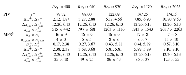
) dataset. All relevant experimental measures are summarized in table 1.
Experimental details of the synchronized PIV and MPS
 $^3$
measurements. The given measures are the inner-scaled wall-normal distance of the PIV measurements (
 $y^+$
), the initial data resolution in streamwise and spanwise direction prior to interpolation onto the DNS grid (
 $\Delta x^+, \Delta z^+$
) and after interpolation (
 $\Delta x^+_{int}, \Delta z^+_{int}$
), the data extent after interpolation (
 $x^+_{int} \times z^+_{int}$
), the original number of wall-shear stress vectors prior to interpolation (
 $n_x \times n_z$
) and after interpolation (
 $n_{x,int} \times n_{z,int}$
), and the micropillar diameter (
 $D_p^+$
) and length (
 $L_p^+$
) in inner units. The
 $+$
sign denotes scaling in wall units and the subscript
 $(\cdot )_{int}$
indicates the interpolated quantities used during inference with the deep learning framework.

Sketch of the experimental set-up comprising simultaneous and synchronized stereo PIV and MPS
 $^3$
measurements in fully developed TCFs. The PIV measurement plane is located at
 $y^+ \approx 3.9 \sqrt {Re_\tau }$
parallel to the channel wall and illuminated by a pulsed laser light sheet. Two cameras with Scheimpflug adapters are focused onto the measurement plane. Simultaneously, two cameras equipped with microscope lenses observe the MPS
 $^3$
in a top view using a shared beam splitter. The MPS
 $^3$
is illuminated in a backlight set-up using an LED with a distinctly different wavelength than the laser light. Thus, by using bandpass filters for all cameras, both measurement systems are optically separated.

The experimental set-up is sketched in figure 2 and is similar to the set-up introduced in Mäteling et al. (Reference Mäteling, Klaas and Schröder2020b
). Stereoscopic PIV measurements in a wall-parallel plane at
 $y^+ \approx 3.9 \sqrt {Re_\tau }$
are synchronized with wall-shear stress measurements using the MPS
 $^3$
(Große & Schröder Reference Große and Schröder2008, Reference Große and Schröder2009; Nottebrock et al. Reference Nottebrock, Klaas and Schröder2012; Geurts et al. Reference Geurts, Nottebrock and Schröder2014; Liu et al. Reference Liu, Klaas and Schröder2019; Mäteling et al. Reference Mäteling, Klaas and Schröder2020b
). The sensor consists of flexible, cylindrical structures (‘micropillars’), which are immersed in the viscous sublayer and bend due to the experienced fluid forces. A preceding calibration relates the micropillar deflection to the instantaneous wall-shear stress. Further details on the measurement principle and the data postprocessing are described in Mäteling et al. (Reference Mäteling, Klaas and Schröder2020b
).
The PIV set-up consists of two Photron FASTCAM SA3 high-speed cameras equipped with Scheimpflug adapters and
 $100$
 $\rm mm$
F/
 $2.0$
Zeiss macro lenses. The cameras are synchronized to a Quantronix Darwin Duo 100 high-speed laser operated at a frame rate of
 $2000$
Hz. Two different MPS
 $^3$
sensors are used to ensure that the micropillars are embedded within the viscous sublayer and possess adequate sensitivity to the flow conditions for all configurations. Thus, for
 $Re_\tau \approx 400, 610, 970$
, the MPS
 $^3$
consists of
 $n_x \times n_z = 16 \times 9$
micropillars with a height of
 $L_p = 300$
 $\unicode{x03BC}\rm m$
and a diameter of
 $D_p = 22$
 $\unicode{x03BC}\rm m$
equidistantly spaced by
 $L_p$
in streamwise and spanwise direction. For
 $Re_\tau \approx 1470$
and
 $2025$
, the micropillar length is reduced to
 $L_p = 200$
 $\unicode{x03BC}\rm m$
with a diameter of
 $D_p = 14$
 $\unicode{x03BC}\rm m$
and
 $n_x \times n_z = 17 \times 8$
micropillars. The pillar-tip deflection is observed in a top view by two pco.dimax HS4 high-speed cameras equipped with K2/SC long-distance microscope lenses. Due to spatial constraints, a splitter cube is used for optical access. The MPS
 $^3$
is illuminated by a pulsed high-power light-emitting diode (LED) system LPS V3 in a backlight configuration at a frame rate of
 $1000$
Hz. Since PIV processing requires an image pair but the MPS
 $^3$
relies on only a single image, which is compared with the reference image at zero flow, its frame rate is halved. To optically separate both measurement systems, the laser and the LED are operated at different wavelengths and the cameras are equipped with corresponding bandpass filters. In total,
 $1000$
data samples are recorded for each configuration.
The PIV data are evaluated with PascalPIV (Marquardt et al. Reference Marquardt, Klaas and Schröder2019, Reference Marquardt, Klaas and Schröder2020) using a multigrid approach with a final interrogation window size of
 $16 \times 16$
pixel
 $^2$
and an overlap of
 $75$
%. This results in a final velocity vector spacing of
 $4 \times 4$
pixel
 $^2$
, the physical resolution of which is given in table 1 for all five Reynolds numbers. For the wall-shear stress measurements, a postprocessing as described in Mäteling et al. (Reference Mäteling, Klaas and Schröder2020b
) is applied and the resulting data sizes and resolutions are provided in table 1. In a final step, all datasets are interpolated onto the same grid as the numerical TCF data (
 $\Delta x^+ = 12.26$
,
 $\Delta z^+ = 6.13$
) using cubic splines since a consistent physical resolution is required for inference. The interpolation of the wall-shear stress values results in distributions of
 $n_{x,int} \times n_{z,int} = 4 \times 3$
values for the lowest Reynolds number and
 $n_{x,int} \times n_{z,int} = 11 \times 10$
for the highest Reynolds number. Although these fields do not cover the entire spatial domain, their spatial information is sufficient to verify the physical significance of the neural wall-shear stress predictions.
2.4. Comparison between numerical and experimental datasets
Although the experiments were targeted to resemble the flow conditions of the numerical data, small inaccuracies and uncertainties are unavoidable in experimental settings. Therefore, we briefly highlight the most significant differences between both datasets for the TCFs at
 $Re_\tau \approx 1000$
. This provides a clear foundation for assessing the performance of the neural architecture with respect to the zero-shot applicability to experimental data.
Since both datasets capture a fully developed TCF, any influence of the inflow conditions is negligible. The experimental facility features an aspect ratio of
 $20$
such that the channel’s sidewalls do not influence the flow along the centreline where the measurements were conducted. Periodic boundary conditions in the DNS exclude sidewall effects too. The friction Reynolds number of the DNS is
 $Re_\tau \approx 1000$
, whereas the experimental dataset captures the flow field at
 $Re_\tau \approx 970$
. Moreover, a small offset of the wall-normal position of the wall-parallel velocity fields exists (
 $y^+ = 123.38$
in the DNS and
 $y^+ = 122.09$
in the experiments). These differences result in a slight discrepancy in the mean velocity values, with
 $\overline {u}^+ \approx 15.5$
observed in the experiments and
 $\overline {u}^+ \approx 16.9$
in the DNS.
Comparison of statistical metrics of the outer-layer velocity fluctuations of the numerical and the experimental TCF at
 ${Re_\tau \approx 1000}$
. Panels (i) present probability density functions (PDFs) of the inner-scaled streamwise fluctuations (a) and violin plots of the r.m.s. (b). Panels (ii) display the two-point correlations in the streamwise (a) and spanwise (b) directions. All statistical metrics indicate a profound similarity between both datasets.

Premultiplied power spectra of the streamwise velocity fluctuations of the TCF at
 ${Re_\tau \approx 1000}$
decomposed into modal representations using the 2-D NA-MEMD. The 2-D NA-MEMD is applied to the streamwise velocity fluctuations of the numerical and the experimental datasets to perform a simultaneous, scale-based decomposition into modal representations (intrinsic mode functions (IMFs)). Sorted with respect to the inherent scale sizes, the IMFs reveal which range of scales are common between both datasets and how their energetic content behaves. By subsequently applying a fast Fourier transform (FFT) to all IMFs, squaring the absolute value of the resulting Fourier coefficients, and taking the mean (lines) and the standard deviation (shaded regions) across all samples, the inner-scaled premultiplied power spectra given in this figure are obtained. Panels (a) provide spectra as a function of the streamwise wavelengths
 $\lambda _x^+$
and (b) as a function of the spanwise wavelengths
 $\lambda _z^+$
. From (i) to (iv), each row shows the spectra related to a different IMF, i.e. a different range of scales, with (i) representing the smallest and (iv) the largest scales. The most distinct difference between experimental and numerical spectra occurs in IMF
 $1$
, in which very small wavelengths of the experimental data comprise a significant amount of energy. This non-physical energy redistribution arises due to measurement noise and also slightly impacts the statistics of IMF
 $2$
.

To provide a statistical analysis of the variations within the outer-layer velocity fields, figure 3 presents the PDFs, the distributions of the root mean square (r.m.s.), and the two-point correlations in both spatial directions. While the distributions of the PDFs and the two-point correlations agree very well, small differences can be observed in the r.m.s.. In addition, we apply the 2-D noise-assisted multivariate empirical mode decomposition (2-D NA-MEMD) (Mäteling & Schröder Reference Mäteling, Klaas and Schröder2020a ) to study the scale distribution in greater detail. In essence, the 2-D NA-MEMD decomposes the velocity fields into scale-based modal representations, which are called IMFs, using a data-driven iterative procedure. By simultaneously decomposing the numerical and the experimental data, we ensure that the resulting IMFs capture the same range of scales and reveal similarities as well as differences between numerical and experimental distributions. Thus, we can analyse which range of scales possesses the largest difference, e.g. due to measurement noise or bias. More details regarding the 2-D NA-MEMD and its application to fluid flow data can be found in Mäteling & Schröder (Reference Mäteling and Schröder2022a ), Lagemann et al. (Reference Lagemann, Albers, Lagemann and Schröder2024, Reference Lagemann, Brunton and Lagemann2024b ) and Mäteling et al. (Reference Mäteling, Albers and Schröder2023).
Figure 4 shows the respective inner-scaled premultiplied power spectra
 $1/\lambda ^+$
 $\Phi ^+_{u'u'}$
of the IMFs. They are calculated using the FFT of the streamwise velocity fluctuations in wall units
 $u'^{+}$
and squaring the absolute values of the resulting Fourier coefficients to obtain the respective energy values
 $\Phi ^+_{u'u'}$
. Those power spectra are premultiplied by the inverse of the inner-scaled wavelengths
 $1/\lambda ^+$
(in streamwise and spanwise direction, respectively) and averaged across the entire datasets, with the corresponding standard deviations indicated by the shaded regions. They are provided in figure 4 as a function of the streamwise
 $\lambda _x^+$
and the spanwise
 $\lambda _z^+$
wavelengths. This representation reveals a significant amount of small-scale measurement noise inherent to the experimental data, which manifests in the first IMF. With increasing scale size, i.e. higher mode number, the difference between numerical and experimental datasets decreases. Thus, the most severe variation is rooted in the smallest scales. Although the spatial resolution of the experimental dataset is higher than the DNS resolution, it does not necessarily mean that the small scales are well resolved. The resolution of the physical features depends on the chosen pulse distance of the PIV measurements, which determines how far the particles have travelled between the first and the second exposure. If the measurements target the governing large-scale flow dynamics, which was the focus of this set-up, this comes at the cost of loosing small-scale information.
3. Deep learning architecture
The proposed framework is a neural operator network based on a convolutional autoencoder architecture, which is sketched in figure 5. A wall-parallel streamwise velocity fluctuation field of dimensions
 $128 \times 128$
pixel
 $^2$
(
 $x^+ \times z^+ \approx 1570 \times 785$
) is evaluated by the network, which outputs the corresponding streamwise wall-shear stress fluctuation field with the same dimension and spatial resolution. Please note that the framework can also be used to estimate the total wall-shear stress when the total velocity is used as the network input. The results of this approach are presented in Appendix B.
Sketch of the proposed deep learning architecture. A streamwise velocity field is evaluated by the autoencoder, which predicts the corresponding wall-shear stress field at the same image resolution. The velocity field is first encoded by a stem block, followed by three basic modules. Each module consists of several basic blocks and the ReLU activation function is omitted at the last stage of each module. During decoding, each basic module starts with an interpolation layer to double the image dimension. The three decoder basic modules are followed by a head block, which outputs the wall-shear stress prediction. The network is trained in a supervised fashion using a loss function based on the L
 $2$
norm between ground truth and prediction. The output dimension of each module is indicated using the following notation: spanwise
 $\times$
streamwise image dimension in the upper row, feature space dimension in the lower row. Abbreviations: convolution (Conv); batch normalization (BN); rectified linear unit (ReLU); max pooling (MaxPool); transposed convolution (ConvT). The kernel size of the convolutions is provided after the convolution operator.

The input is first processed by a stem block, which includes a convolution with a kernel size of
 $7 \times 7$
and a stride of
 $2$
, followed by a batch normalization, ReLU activation and max pooling with a kernel size of
 $3$
and a stride of
 $2$
. The output of the stem block is a spatially compressed matrix of
 $32 \times 32$
pixel
 $^2$
with
 $128$
feature maps. It is then processed by several basic blocks, which contain a convolution with a kernel size of
 $3 \times 3$
, a batch normalization, and ReLU activation. The first basic block of each module (same-sized basic blocks in figure 5 build a module) applies a convolution with a stride of
 $2$
and a doubling of the feature space, whereas the subsequent blocks have a stride of
 $1$
, retaining the spatial dimension using zero-padding, and preserve the feature space dimension. The ReLU activation is omitted at the output of each module. The compressed latent representation has a spatial dimension of
 $4 \times 4$
pixel
 $^2$
with
 $1024$
feature maps. Each module of the decoder contains a preceding interpolation layer, which upsamples the spatial dimension by a factor of
 $2$
using nearest neighbours interpolation. Our studies showed that this type of upsampling in the early stages of decoding improves the resolution of small-scale features compared with the often used transposed convolution. All basic blocks of the decoder have a stride of
 $1$
and the first basic block in each module halves the feature space. In the final stage, the head block performs three transposed convolutions with subsequent ReLU activation except for the final output. The network is trained in a supervised fashion using the L
 $2$
norm between the wall-shear stress prediction and the ground truth as the training loss. The same loss is used to assess the network’s performance during inference with numerical and experimental test data.
The exact number of basic blocks contained in each encoding and decoding module is the result of a hyperparameter study. The encoder performs best with four basic blocks in the first two basic modules and two basic blocks in the third module. For the decoding path, we employ four basic blocks in each network stage, resulting in a total of
 $26$
hidden layers and
 $40\,345\,729$
trainable parameters. Moreover, we studied the impact of using residual layers within each module (ResNet) as well as cross-connections between the encoder and decoder (Unet). By fine-tuning each of these networks with hyperparameter studies, we achieved a similar performance across all architectures. For the sake of readability, we therefore only discuss results related to the basic autoencoding architecture and provide further details and comparisons with respect to the other architectures in Appendix C.
The network training is performed on four NVIDIA A100 graphics processing units (GPUs). We used a batch size of
 $7$
per GPU, i.e.
 $28$
in total, and a dropout ratio of
 $0.3$
to prevent overfitting. An Adam optimizer with an initial learning rate of
 $9.7 \times 10^{-5}$
and weight decay of
 $1.7 \times 10^{-4}$
was combined with a scheduler that reduces the learning rate by a factor of
 $0.2$
when the validation loss is not improving after
 $10$
epochs. In total, training was performed for
 $500$
epochs with a minimum learning rate of
 $10^{-10}$
. All training specific parameters have been optimized using extensive hyperparameter studies.
Two different training set-ups are used in the present study. First, we solely train the neural network on the TCF data at
 $Re_\tau \approx 1000$
to investigate the capabilities of the network in the optimal setting (i.e. only a single flow condition). Second, we use all three configurations, i.e. the TCF and both TBL flows, to analyse the generalization ability of the network across flow conditions and slightly changing flow problems (statistically one-dimensional versus statistically developing flow in streamwise direction). For the first scenario, the numerical TCF dataset described in § 2.1 is randomly divided into a training dataset containing
 $80$
% of the snapshots (
 $7680$
samples), a validation dataset comprising
 $10$
% of the snapshots (
 $960$
samples), and a test dataset with the remaining
 $10$
% (
 $960$
samples). While a validation is performed at the end of each epoch, the test dataset is only used after the entire training procedure is terminated. Thus, it serves as a verification for the network performance on unseen in-distribution data samples.
In the second scenario, we use data from all three numerical simulations, i.e. the TCF at
 $Re_\tau \approx 1000$
and the TBL flows at
 $Re_\tau \approx 390$
and
 $1500$
, with the same percentage distribution between training, validation and test samples as for the single configuration (
 $80$
%,
 $10$
%,
 $10$
%). To avoid any bias during training, the same number of samples is taken from each dataset. Thus,
 $4164$
samples randomly selected from each dataset are used for training (
 $12\,492$
in total) and
 $516$
(
 $1548$
in total) for validation and testing, respectively.
4. Results
In the following, the discussion of the results is split into two main segments. In § 4.1, we evidence the successful performance of the proposed neural network when trained on a single configuration, i.e. the TCF at
 $Re_\tau \approx 1000$
. In § 4.2, we demonstrate that our deep learning architecture accurately predicts wall-shear stress distributions when trained on a comprehensive dataset that unifies flow fields of different configurations, i.e. TCF and TBL flows at three different Reynolds numbers spanning
 $390 \leqslant Re_\tau \leqslant 1500$
. Moreover, we demonstrate the zero-shot transferability to out-of-distribution experimental data to evidence the strong generalizability and effectiveness in real-world measurements.
4.1. Wall-shear stress predictions of the TCF at
 $Re_\tau \approx 1000$

This section presents the results of the deep learning framework solely trained on the numerical TCF data at
 $Re_\tau \approx 1000$
. Section 4.1.1 demonstrates that the network is able to provide accurate in-distribution wall-shear stress predictions based on the numerical test dataset. In § 4.1.2, we show that the network also reliably predicts wall-shear stress distributions from experimental PIV velocity measurements.
4.1.1. In-distribution results of the numerical data
Figure 6 provides an example of an input, i.e. a streamwise velocity fluctuation field, a network output, i.e. the prediction of the wall-shear stress fluctuation field, the true wall-shear stress fluctuations and the error in the network prediction for an arbitrary sample of the test dataset. This example shows how well the network predicts a physically correct wall-shear stress distribution for unseen data (recall that the test dataset was never provided during network training and validation).
Velocity and wall-shear stress fluctuation fields of an arbitrary sample of the numerical test dataset of the TCF at
 ${Re_\tau \approx 1000}$
, scaled in wall units. (a) Inner-scaled streamwise velocity fluctuations (network input), (b) true inner-scaled wall-shear stress fluctuations, (c) prediction error, (d) predicted wall-shear stress fluctuations (network output). The comparison between ground truth (b) and predicted (d) wall-shear stress shows that the proposed architecture provides physically correct wall-shear stress fields from unseen velocity fields. This is further evidenced by the low prediction error, which is calculated using the absolute difference between true and predicted wall-shear stress values.

Statistical assessment of the wall-shear stress predictions of the numerical test dataset of the TCF at
 ${Re_\tau \approx 1000}$
. Panels (i), from (a) to (c), present violin plots of the correlation coefficient
 $R$
between the true and predicted wall-shear stress, the mean squared error (MSE), and the r.m.s. of the true and predicted data. Panels (ii), from (a) to (c), display the PDFs and the two-point correlations in the streamwise (
 $x$
) and spanwise (
 $z$
) directions. All statistical metrics indicate a highly accurate estimation of the wall-shear stress fluctuations.

For a statistical assessment of the network’s predictive performance, figure 7 provides statistical metrics comparing the prediction with the true wall-shear stress for the entire test dataset. The Pearson correlation coefficient, as depicted in the violin plot in figure 7(ai), has a median value of
 $R = 0.9963$
. Meanwhile, the MSE between the prediction and the ground truth, as shown in the violin plot in figure 7(bi), has a median value of
 $5.32 \times 10^{-4}$
. The comparison between the violin plots of the r.m.s. of the predicted and the true wall-shear stress (figure 7
ci) as well as the PDFs (figure 7
aii) and the two-point correlations in the streamwise (figure 7
bii) and spanwise (figure 7
cii) directions show an excellent agreement, demonstrating the high prediction accuracy.
Modal representations of the true and the predicted wall-shear stress fields of the test sample presented in figure 6, scaled in wall units. Panel (a) contains the IMFs of the true wall-shear stress, (b) depicts the IMFs related to the predicted wall-shear stress, and (c) shows the reconstruction error. Panels (i) contain the initial wall-shear stress fields and the corresponding prediction error (prior to applying the 2-D NA-MEMD), which are identical to the data in figure 6. Although all scales are predicted very accurately by the deep learning framework, the prediction error slightly increases with smaller scale size.

To assess the network’s performance in greater detail, we apply the 2-D NA-MEMD (Mäteling & Schröder Reference Mäteling and Schröder2022a
) to the wall-shear stress predictions and ground truth distributions and subsequently perform an FFT on each mode to inspect the power spectra. By simultaneously decomposing the ground truth and the prediction of each sample, we ensure that the resulting IMFs capture the same range of scales. This allows us to assess the prediction capabilities of the network in a scale-based representation. In other words, we can analyse if there is a certain bias in the prediction of specific scales or if a certain range of scales is more difficult to obtain with our deep learning architecture. Figure 8 provides an example of the obtained modes of the true and the predicted wall-shear stress distributions of the same test sample shown in figure 6. It is obvious that the largest deviation – which is still small in an overall sense – occurs in the first mode, which comprises the smallest scales. The same tendency can be observed in the inner-scaled premultiplied power spectra of the IMFs, which are given in figure 9 as a function of the streamwise
 $\lambda _x^+$
and the spanwise
 $\lambda _z^+$
wavelengths. The figure depicts the spectra averaged over the entire test dataset and the standard deviation across all samples is provided as a shaded area, proving that the proposed framework provides very accurate wall-shear stress estimates. Only a small deviation between ground truth and network prediction can be observed in the first mode for small streamwise wavelengths. This behaviour is not uncommon for networks because they tend to learn large features very well, whereas the small-scale content, which varies most significantly across all samples, is most challenging to be represented reliably.
Premultiplied power spectra of the IMFs of the wall-shear stress predictions and ground truth distributions of the numerical test dataset of the TCF at
 ${Re_\tau \approx 1000}$
. Panels (i) provide spectra as a function of the streamwise wavelengths
 $\lambda _x^+$
and panels (ii) as a function of the spanwise wavelengths
 $\lambda _z^+$
. From (a) to (d), each row shows the spectra related to a different IMF, i.e. a different range of scales, with (a) representing the smallest and (d) the largest scales. Lines indicate spectra averaged over all samples and the shaded regions are the corresponding standard deviations. On a statistical basis, the power spectra evidence how well the network predicts correct wall-shear stress values across all scales. Only a very small deviation can be observed for the smallest scales in IMF1.

In view of the current application, the information about the large-scale wall-shear stress features is already comprised in the velocity field provided as the network input. Extensive studies in the literature (Marusic & Heuer Reference Marusic and Heuer2007; Agostini & Leschziner Reference Agostini and Leschziner2014; Marusic et al. Reference Marusic, Baars and Hutchins2017; Pathikonda & Christensen Reference Pathikonda and Christensen2019; Mäteling & Schröder Reference Mäteling and Schröder2022a ) have shown how the large-scale dynamics of the outer layer are superimposed onto the near-wall flow. Thus, the deep learning framework is essentially a model of the various physical processes involved in this inner–outer interaction. In other words, it can be viewed as a neural operator network, which learns a physically accurate transfer function from the large-scale flow features of the outer-layer velocity field to the wall-shear stress distribution. Moreover, figures 8 and 9 show that the proposed architecture is able to learn a physically meaningful representation of other scales as well (with inaccuracies at the smallest scales, i.e. IMF 1). Most likely, this is rooted in the fact that physical connections between the inner and the outer layer also exist within these scales, but which have been studied less intensely so far because of their less significant impact on the governing near-wall dynamics. However, the smallest scales in turbulent wall-bounded flows have a statistically universal character (Marusic et al. Reference Marusic, Mathis and Hutchins2010a ), which means that it is nearly impossible to trace back their origin. Thus, information about the very small-scale behaviour of the wall-shear stress cannot be extracted from the outer-layer velocity fields. Therefore, there is a certain inaccuracy in their prediction. However, since these scales have the smallest impact in an energetic sense and are therefore less important for, e.g. drag reduction concepts and life time estimation of structural materials, a minor uncertainty in their correct prediction is acceptable for the majority of applications.
Thus, in summary, the proposed deep learning architecture performs exceptionally well in predicting wall-shear stress fluctuations from outer-layer velocity fluctuation fields for in-distribution numerical data.
4.1.2. Zero-shot application to experimental data
The zero-shot applicability of the deep learning framework to experimental data is evidenced with the pretrained network discussed in § 4.1.1. This neural network is solely trained on DNS data and first exposed to experimental data during testing, i.e. after the training is completed. Figure 10 shows the experimental input, i.e. the PIV-based velocity fluctuation field, and the predicted wall-shear stress distribution for arbitrary experimental test samples. In addition, the true wall-shear stress distribution measured by the MPS
 $^3$
is provided next to an enlarged extract of the predicted wall-shear stress field matching the experimentally measured region. The comparison shows a good agreement between prediction and ground truth indicating that the network is able to generalize well to experimental conditions without being explicitly trained on an experimental dataset. Some of the predictions appear smoother compared with the measured wall-shear stress fields due to small-scale measurement uncertainties in the MPS
 $^3$
data.
Velocity and wall-shear stress fluctuation fields of arbitrary samples of the experimental dataset of the TCF at
 ${Re_\tau \approx 1000}$
, scaled in wall units. Panel (a) shows the inner-scaled streamwise velocity fluctuations obtained from the PIV measurements (network input), (b) depicts the experimental wall-shear stress predictions (network output), and (c) and (d) present the predicted and MPS
 $^3$
based wall-shear stress in a spatially limited extract. This comparison shows that the network is able to predict physically meaningful wall-shear stress fields from experimental velocity measurements although it was never trained on the particular characteristics of these measurements.

Going beyond visualizations of instantaneous results, figure 11 presents statistical metrics comparing the experimental predictions and the measured wall-shear stress distributions. The violin plot of the correlation coefficient displays a very high correlation with a median value of
 $R = 0.9889$
. Consequently, the MSE is very low with a median value of
 $3.42 \times 10^{-4}$
. The distributions of the r.m.s., the PDF and the two-point correlations match very well between predicted and measured wall-shear stress, which indicates a successful application of our deep-learning framework to experimental data in a statistical sense. Please note that the two-point correlations only show a small spatial extent since the area measured with the MPS
 $^3$
is limited. Similarly, this limited field of view results in slightly different distributions of the PDF and the r.m.s. compared with the full-domain numerical results shown in figure 7.
Statistical assessment of the wall-shear stress predictions of the experimental dataset of the TCF at
 ${Re_\tau \approx 1000}$
. A detailed description of the statistical metrics is provided in the caption of figure 7. All quantities indicate a highly accurate estimation of the wall-shear stress.

Premultiplied power spectra of the IMFs of the numerical and experimental wall-shear stress predictions as well as the numerical ground truth distributions of the TCF at
 ${Re_\tau \approx 1000}$
. Panel (a) provides spectra as a function of the streamwise wavelengths
 $\lambda _x^+$
and panel (b) as a function of the spanwise wavelengths
 $\lambda _z^+$
. From (i) to (iv), each row shows the spectra related to a different IMF, i.e. a different range of scales, with (i) representing the smallest and (iv) the largest scales. Lines indicate spectra averaged over all samples and the shaded regions are the corresponding standard deviations. Please note that the numerical data were already shown in figure 9 and are included for comparison since the statistics of the numerical and the experimental datasets are expected to match. This comparison reveals that the network predictions based on experimental velocity fields are slightly inaccurate with respect to the energetic content of the smallest scales (IMF
 $1$
). This is rooted in the small-scale noise inherent to the experimental velocity measurements (see figure 4), which is incorrectly processed by the neural network. However, the overall trend of the experimental spectra, especially for medium-size and large-scale flow features, is very similar to the numerical data evidencing a successful performance of the deep learning framework in the noisy flow conditions of the experimental dataset.

To provide further details on the experimental predictions, especially with respect to medium-size and large-scale flow structures that are not captured in the MPS
 $^3$
data due to the limited field of view, we apply the 2-D NA-MEMD with subsequent FFT to the true numerical, the predicted numerical and the predicted experimental wall-shear stress fields. Please note that the results related to the numerical data are already given in figure 9. They are included in figure 12 for comparison since the statistics of the experimental estimates are expected to match the numerical statistics if the deep learning framework performs as intended. A distinct difference in the power spectra can be observed for the smallest scales, i.e. in IMF1, as well as in the low-wavelength regime of the streamwise spectra of IMF2. The experimental wall-shear stress predictions are not as accurate as the numerical predictions, which results from the small-scale measurement noise inherent to the experimental velocity measurements (see figure 4). The network is not able to adequately process this information since it was not comprised in the training data distribution, which yields a marginal redistribution of the energetic content. However, we have to acknowledge that these deviations are only within a few per cent and the confidence intervals of the numerical and experimental spectra show a substantial overlap. Moreover, the predictions of the medium- and large-scale wavelengths are very accurate. Therefore, we conclude that the proposed architecture is able to estimate physically meaningful wall-shear stress distributions from experimental velocity fields although the training was solely performed with DNS data. It is especially worth mentioning that some of the characteristics of the experimental dataset differ from the numerical dataset as discussed in § 2.4, with the small-scale measurement noise being the most significant source of variation. Nevertheless, the deep learning framework is able to provide reliable instantaneous (figure 10) and statistical (figures 11 and 12) information about the experimental wall-shear stress.
4.2. Wall-shear stress predictions of the multiconfiguration network using TCF and TBL flows at various Reynolds numbers
In the following, we show that our proposed deep learning architecture predicts reliable wall-shear stress distributions when trained on a comprehensive dataset that unifies flow fields of different configurations. On the one hand, we evidence a successful performance with respect to in-distribution wall-shear stress predictions using the numerical test data. On the other hand, we present a successful zero-shot application to experimental TCFs at several Reynolds numbers. Besides the three Reynolds numbers covered in the training dataset (two of which were related to spatially developing TBL flows and not to fully developed TCF), the network also performs well on an intermediate and an extrapolated Reynolds number. In Appendix B, we further demonstrate that this framework can also be utilized to predict the total wall-shear stress, rather than just the wall-shear stress fluctuations, if desired for a specific application.
Velocity and wall-shear stress fluctuation fields of arbitrary samples of the numerical test datasets, scaled in wall units. From (a) to (d), each row contains the inner-scaled streamwise velocity fluctuations (network input), the true inner-scaled wall-shear stress fluctuations, the predicted wall-shear stress fluctuations (network output), and the prediction error, which is the absolute deviation between ground truth and prediction. From (i) to (iii), the data correspond to the TBL flow at
 $Re_\tau \approx 390$
, the TCF at
 $Re_\tau \approx 1000$
and the TBL flow at
 $Re_\tau \approx 1500$
. For all configurations, the true and the predicted wall-shear stress distributions match very well and the reconstruction error shows only small-scale irregularities in predicting the true physics (please note the different colourbar limits).

On an instantaneous level, figure 13 shows that the neural network derives accurate wall-shear stress fields for all three configurations. Using arbitrarily selected test samples of the numerical data, each row of figure 13 depicts the input velocity fluctuation field, the true and the predicted wall-shear stress fluctuation fields, and the reconstruction error for the TBL flow at
 $Re_\tau \approx 390$
(figure 13
ai, bi, ci, di), the TCF at
 $Re_\tau \approx 1000$
(figure 13
aii, bii, cii, dii), and the TBL flow at
 $Re_\tau \approx 1500$
(figure 13
aiii, biii, ciii, diii). The reconstruction errors indicate that the inaccuracy in the prediction is primarily based on small-scale features, which was already observed for the single-configuration setting discussed in § 4.1. In Appendix A.3, we further demonstrate an accurate prediction of the temporal wall-shear stress dynamics for a time-resolved dataset.
Velocity and wall-shear stress fluctuation fields of arbitrary samples of the experimental TCFs at various Reynolds numbers, scaled in wall units. Panel (a) shows the inner-scaled streamwise velocity fluctuations obtained from the PIV measurements (network input), (b) depicts the experimental wall-shear stress predictions (network output), and (c) and (d) present the predicted and measured wall-shear stress in a spatially limited extract. From (i) to (v), the Reynolds number increases from
 $Re_\tau \approx 400$
to
 $Re_\tau \approx 2000$
. Even though the training dataset contains only a single numerical configuration of a TCF at
 $Re_\tau \approx 1000$
, the network also successfully predicts the wall-shear stress fields at the two TBL related Reynolds numbers of
 $Re_\tau \approx 390$
and
 $Re_\tau \approx 1500$
. Moreover, the interpolated configuration at
 $Re_\tau \approx 600$
and the out-of-distribution Reynolds number of
 $Re_\tau \approx 2000$
can reliably be covered by the deep learning framework.

Figure 14 presents instantaneous results with respect to the experimental configurations. Each row represents one Reynolds number and displays the PIV based velocity fluctuation fields, the predicted wall-shear stress fluctuation fields, and an extract of the former that matches the location and size of the MPS
 $^3$
based true wall-shear stress distribution. For lower Reynolds numbers, the field of view covered by the PIV measurements is smaller compared with the physical size of the training data. Therefore, the respective velocity and wall-shear stress fields are smaller. Since the deep learning architecture is based on convolutional layers with a small receptive field, a varying input size does not impact the network’s performance. The instantaneous results in figure 14 evidence a physically meaningful wall-shear stress prediction across all Reynolds numbers. Although the training data contain solely TBL flows at
 $Re_\tau \approx 390$
and
 $Re_\tau \approx 1500$
, the network reliably predicts wall-shear stress fields from TCF related velocity fields at those Reynolds numbers. Moreover, it is able to provide an accurate estimate for a Reynolds number of
 $Re_\tau \approx 600$
, which was not part of the training dataset but is within the covered Reynolds number range. Fortunately, we also observe a successful performance at
 $Re_\tau \approx 2000$
, which constitutes a significant extrapolation from the highest Reynolds number of
 $Re_\tau \approx 1500$
included in the training dataset. This suggests that the network has effectively learned the underlying physical principles, capturing essential features that are consistent across different flow regimes. This enables a generalization beyond the range of the training data. However, this capability is likely limited to flow conditions with similar physical characteristics and may not extend to significantly higher Reynolds numbers or flows with intense pressure gradients.
Statistical assessment of the wall-shear stress predictions using the multiconfiguration network with the numerical test dataset of the TCF at
 ${Re_\tau \approx 1000}$
. A detailed description of the statistical metrics is provided in the caption of figure 7.

Measuring the outer-layer velocity fields precisely at
 $y^+ = 3.9 \, \sqrt {Re_\tau }$
in experimental settings may pose a challenge. Therefore, in Appendix A.4, we present inference results obtained from velocity fields at various wall-normal locations, which demonstrate that even a deviation of
 $10\,\%$
still provides meaningful wall-shear stress predictions.
Beyond visualizing instantaneous results, figure 15 presents statistical metrics comparing the predictions of the numerical test data of the TCF at
 $Re_\tau \approx 1000$
with the true wall-shear stress distributions. The violin plot of the correlation coefficient demonstrates a high correlation with a median value of
 $R = 0.9782$
. Consequently, the MSE is notably low, with a median value of
 $3.08 \times 10^{-3}$
. Both metrics indicate a slight performance decline compared with the single-configuration network discussed in the previous section. This suggests that generalizing across different flow conditions results in a minor reduction in prediction accuracy. However, overall, the statistical measures are highly favourable and also the distributions of the r.m.s., the PDF and the two-point correlations align closely between predicted and true wall-shear stress. Thus, the multiconfiguration network provides physically meaningful wall-shear stress fluctuations for unseen in-distribution data. The statistical results of the two TBL flows are provided in Appendix A.1 and demonstrate a similar accuracy of the network’s predictions.
Statistical assessment of the wall-shear stress predictions of the experimental dataset at
 ${Re_\tau \approx 600}$
using the multiconfiguration network. A detailed description of the statistical metrics is provided in the caption of figure 7.

Figure 16 presents the same statistical metrics for the experimental dataset at
 $Re_\tau \approx 600$
, i.e. the interpolated configuration. All plots underscore the high accuracy of the experimental wall-shear stress predictions. The corresponding results for all other experimental test cases are provided in Appendix A.1 and confirm that the multiconfiguration network accurately predicts wall-shear stress fluctuation fields for in-distribution, interpolated and extrapolated configurations.
Next, we investigate the premultiplied power spectra obtained by applying an FFT to the 2-D NA-MEMD based modal representations of the test data. Figure 17 provides the statistics of the TCF at
 $Re_\tau \approx 1000$
, while the spectra of the two TBL flows are provided in Appendix A.2. In figure 17, the spectra of the ground truth, the predictions based on the numerical test data and the predictions based on the experimental data are given as a function of streamwise and spanwise wavelengths.
Premultiplied power spectra of the IMFs of the numerical and experimental wall-shear stress predictions of the multiconfiguration network as well as the numerical ground truth distributions at
 ${Re_\tau \approx 1000}$
. Panel (a) provides spectra as a function of the streamwise wavelengths
 $\lambda _x^+$
and (b) as a function of the spanwise wavelengths
 $\lambda _z^+$
. Lines indicate averages over all samples and the shaded regions are the corresponding standard deviations. The predicted wall-shear stress distributions align closely with the ground truth, with the largest discrepancies observed at the smallest scales (IMF1). Generally, the experimental predictions are slightly less accurate than the numerical ones, but they still follow the main trends very well.

Premultiplied power spectra of the IMFs of the experimental wall-shear stress predictions at
 ${Re_\tau \approx 600}$
and
 ${Re_\tau \approx 2000}$
using the multiconfiguration network. Panel (a) provides spectra as a function of the streamwise wavelengths
 $\lambda _x^+$
and (b) as a function of the spanwise wavelengths
 $\lambda _z^+$
. Lines indicate averages over all samples and the shaded regions are the corresponding standard deviations. Although no ground truth information is available for comparison, the overall trends of these spectra are physically meaningful and similar to the other Reynolds numbers shown in figures 17, 25 and 26. Indeed, for these Reynolds numbers and the depicted range of wavelengths, the inner-scaled premultiplied power spectra are expected to collapse (Samie et al. Reference Samie, Marusic, Hutchins, Fu, Fan, Hultmark and Smits2018).

Overall, a very good agreement is observed between the ground truth and the numerical predictions. Only the smallest scales (IMF1), especially with respect to the streamwise wavelengths, are slightly underestimated. The overall trend of the experimental predictions is very similar to the numerical results but with slightly larger deviations across most modes. Specifically the smallest scales possess a higher deviation from the true distribution, which was equally observed for the single-configuration network discussed in § 4.1. By comparing the spectra of the wall-shear stress distributions predicted with the single-configuration network (figure 12) to the multiconfiguration network results (figure 17), we can see a minor increase of the uncertainty within the prediction when the network is trained on several configurations. This is rooted in the fact that this network has to generalize more broadly across flow conditions, i.e. a range of Reynolds numbers, as well as slightly varying characteristics of the TCF and TBL flows, which comes at the cost of accuracy. Nevertheless, the validation with the measurement data on an instantaneous level (figure 14) as well as the power spectra still show a reliable prediction and generalization ability that allows a trustworthy application to experimental data covering a broad range of Reynolds numbers.
Lastly, we analyse the statistics at Reynolds numbers which were not included in the training data. Precisely, the power spectra of the TCF at
 $Re_\tau \approx 600$
(within the covered range) and at
 $Re_\tau \approx 2000$
(extrapolation) are presented in figure 18. Their distributions are very similar to the TCF at
 $Re_\tau \approx 1000$
shown in figure 17 with the largest deviation occurring in IMF1. Although no ground truth information is available for a quantitative comparison, the power spectra of all considered Reynolds numbers are expected to be very similar in the investigated range of wavelengths (Samie et al. Reference Samie, Marusic, Hutchins, Fu, Fan, Hultmark and Smits2018). Therefore, and in view of the good agreement with the instantaneous wall-shear stress measurements (figure 14) and the other statistical metrics (figures 16 and 24), we conclude that the network is able to predict reliable wall-shear stress information for these Reynolds numbers. This ability is a very useful characteristic for prospective applications since the neural architecture does not need to be trained on the exact flow conditions targeted in the experimental measurements. By covering a sufficiently large range of Reynolds numbers and flow problems with enough intermediate stages, our study indicates that interpolation and (reasonable) extrapolation to additional flow configurations is possible. Thus, the proposed neural architecture provides a valuable surrogate model for temporally and spatially resolved wall-shear stress information captured within a large spatial domain to advance future experimental applications.
5. Conclusion
Acquiring experimental wall-shear stress information is of tremendous value for academic and applied research in a variety of disciplines ranging from human medicine to civil aviation. However, experimental measurements of temporally and spatially resolved wall-shear stress dynamics covering a large spatial domain are extraordinarily challenging – often even impossible. In the present work, we provide a deep-learning-based surrogate model which derives instantaneous wall-shear stress distributions from wall-parallel velocity fields located within the logarithmic region. In many settings, velocity measurements in this region are easily conducted using planar PIV. Purely trained on DNS data, our proposed neural architecture outputs reliable wall-shear stress fields from PIV-based velocity fields. We verify the physical significance of these neural predictions with wall-shear stress measurements, which have been synchronized to the PIV measurements, using the MPS
 $^3$
.
Our study is based on fully developed TCFs at friction Reynolds numbers in the range of
 $400 \leqslant Re_\tau \leqslant 2000$
as well as spatially developing TBL flows at
 $Re_\tau \approx 390$
and
 $Re_\tau \approx 1500$
. The velocity fields are extracted in a wall-parallel plane located at
 $y^+ \approx 3.9 \sqrt {Re_\tau }$
because the large-scale flow features are most energetic in this region. Thus, they have the most significant impact on the wall-shear stress dynamics due to the various physical mechanisms involved in the inner–outer interaction inherent to turbulent wall-bounded flows. Using a supervised training approach based on DNS data, the proposed deep learning architecture learns a neural representation of these interaction phenomena such that it is able to extract physically correct wall-shear stress distributions from the provided velocity fields. We demonstrate the successful performance of this framework when solely trained on a single flow problem, i.e. the TCF at
 $Re_\tau \approx 1000$
, as well as a multiconfiguration setting in which TCF and TBL flows at several Reynolds numbers are combined. Furthermore, our deep learning framework demonstrates zero-shot applicability to experimental measurement data of TCFs. Specifically, it provides physically accurate wall-shear stress information from PIV-based velocity fields at various Reynolds numbers without being exposed to the particular characteristics of the measurement data during training. Notably, the framework has proven its predictive capabilities even for Reynolds numbers beyond the scope of the training dataset, including one intermediate and one extrapolated flow condition. This behaviour underscores the robustness of our deep learning architecture and its ability to provide accurate wall-shear stress estimates without the necessity of training on the exact flow conditions, which represents a substantial leap towards achieving true generalizability in fluid dynamics modelling.
The results of this study bear great potential for experimental and numerical fluid dynamics. Being able to use the proposed framework as a surrogate model to obtain experimental wall-shear stress dynamics can advance research in various domains. For example, it allows to experimentally study the efficiency and the involved physical mechanisms of friction drag reduction techniques, which are mainly investigated by numerical methods so far. In this context, it might also be used in experimental feedback control applications where only access to velocity data are available. On the other hand, our framework can advance the experimental in vitro investigation of cardiovascular diseases, in which the temporal dynamics as well as the spatial distribution of the wall-shear stress play a central role in disease development and progression. We aim to amend the network in the future, enhancing its versatility and generalizability to allow such applications to medical problems, which pose certain challenges related to the pulsatile flow and the different physical mechanisms. With respect to numerical simulations, our workflow could support the development of enhanced or novel wall models for wall-modelled large-eddy simulations since it constitutes a purely data-driven representation of the inner–outer interactions, which could generalize more broadly than state-of-the-art analytical models when trained on a variety of different flow conditions.
To enable these prospective advancements, future studies have to focus on the generalization capabilities in a broader setting. So far, we considered two flow problems at various Reynolds numbers, but the physical mechanisms of the inner–outer interactions within TCFs and TBL flows are quite similar. Therefore, it is necessary to extend the framework to a wider range of flow problems with greater variability in the respective flow conditions. This extension could include flows at higher Reynolds numbers, flows subjected to pressure gradients, time-varying inflow conditions and the presence of surface roughness and curved surfaces. Since ground truth information in terms of DNS data might not be available for all these configurations, adopting an unsupervised training approach could be highly beneficial. Additionally, fine-tuning the network’s capability to represent experimental conditions could be achieved through transfer learning. Expanding the data utilized by the network to include spanwise information, in addition to streamwise data, would further enrich the wall-shear stress predictions. An extended framework will also incorporate a revised data normalization method that does not rely on the friction velocity. Currently, this quantity is used to scale the input velocity fields to wall units, providing consistent scaling across various Reynolds numbers to facilitate the network training. However, this poses challenges if the friction velocity is unknown a priori, but can easily be circumvented by using an empirical scaling factor that normalizes the data in a similar range. Moreover, it is certainly of great interest to understand how the neural network transfers outer-layer velocity to wall-shear stress information. Therefore, the application of symbolic regression (Brunton, Proctor & Kutz Reference Brunton, Proctor and Kutz2016; Udrescu & Tegmark Reference Udrescu and Tegmark2020; Udrescu et al. Reference Udrescu, Tan, Feng, Neto, Wu and Tegmark2020) to the latent space could provide an analytical expression of the inherent mapping function, which can subsequently be analysed in a physical context and used for model-based predictive tasks.
Acknowledgements
We like to thank W. Schröder and the Institute of Aerodynamics of RWTH Aachen University for supporting the experimental measurement campaign.
Funding
This research was funded by the German Research Foundation within the Walter Benjamin fellowships MA 10764/1-1 (EL) and LA 5508/1-1 (CL). E.L., C.L. and S.L.B. acknowledge support from the National Science Foundation AI Institute in Dynamic Systems (grant number 2112085) and the Boeing Company. Furthermore, the authors gratefully acknowledge the Gauss Centre for Supercomputing e.V. for funding this project by providing computing time on the GCS Supercomputers.
Declaration of interests
The authors report no conflict of interest.
Data availability statement
Code to reproduce the results of this publication is available at https://github.com/cl126162/DeepWSS-Quant and the source code of the 2-D NA-MEMD can be found in Mäteling & Schröder (Reference Mäteling and Schröder2022b ).
Appendix A. Additional results
This section presents additional validation results of the single- and multiconfiguration networks. Appendix A.1 covers the statistical metrics, i.e. correlation coefficients, MSE, r.m.s., PDF and two-point correlations, of the numerical TBL flows at
 $Re_\tau \approx 390$
and
 $1500$
as well as the experimental datasets at
 $Re_\tau \approx 400$
to
 $2000$
. In Appendix A.2, the scale-based power spectra of the numerical TBL flows and the experimental TCF flows at
 $Re_\tau \approx 390$
and
 $1500$
are shown. Appendix A.3 provides an example of the temporal evolution of the wall-shear stress for time-resolved data. Due to potential uncertainties in precisely localizing the wall-normal position from which the velocity fields are extracted in experimental settings, the effects of off-location inputs during inference are discussed in Appendix A.4 for the TCF at
 $Re_\tau \approx 1000$
. Appendix A.5 demonstrates that training on an outer-layer location farther away from the wall than the optimal location
 $y^+ \approx 3.9 \sqrt {Re_\tau }$
used throughout this analysis results in similarly accurate wall-shear stress predictions. Finally, Appendix A.6 presents results for datasets scaled with the z-score normalization instead of the inner units if the friction velocity is inaccessible.
A.1. Statistical metrics
Figures 19 and 20 present the statistical metrics of the TBL flows at
 $Re_\tau \approx 390$
and
 $1500$
, which have already been discussed in § 4.2 for the numerical test dataset of the TCF at
 $Re_\tau \approx 1000$
. For both TBL datasets, very high Pearson correlation coefficients with median values of
 $R = 0.9793$
(
 $Re_\tau \approx 390$
) and
 $R=0.9601$
(
 $Re_\tau \approx 1500$
) are displayed in figures 19(ai) and 20(ai) as violin plots. Low MSEs with median values of
 $6.48\times 10^{-3}$
and
 $1.34\times 10^{-2}$
, respectively, are presented as violin plots in figures 19(bi) and 20(bi). The violin plots of the r.m.s. (figures 19
ci and 20
ci) show a small deviation between predicted and true wall-shear stress. However, the additional metrics, i.e. PDF (figures 19
aii and 20
aii) and two-point correlations (figures 19
bii, cii and 20
bii, cii), agree very well and thus, demonstrate highly accurate wall-shear stress predictions for unseen data of the TBL flows.
Statistical assessment of the wall-shear stress predictions using the multiconfiguration network with the numerical test dataset of the TBL flow at
 ${Re_\tau \approx 390}$
. Panels (i) from (a) to (c) present violin plots of the correlation coefficient
 $R$
, the MSE and the r.m.s. of the true and predicted data. Panels (ii) from (a) to (c) display the PDFs and the two-point correlations in the streamwise (
 $x$
) and spanwise (
 $z$
) directions. All statistical metrics indicate a highly accurate estimation of the wall-shear stress.

Statistical assessment of the wall-shear stress predictions using the multiconfiguration network with the numerical test dataset of the TBL flow at
 ${Re_\tau \approx 1500}$
. A detailed description of the statistical metrics is provided in figure 19.

Figures 21–24 present the statistics for the experimental TCF datasets for Reynolds numbers of
 $Re_\tau =400$
,
 $1000$
,
 $1500$
and
 $2000$
. The results at
 $Re_\tau =400$
(figure 21) and
 $Re_\tau =1000$
(figure 22) demonstrate a very high accuracy of the experimental wall-shear stress predictions. Small deviations between the true and the predicted data can be observed at
 $Re_\tau =1500$
(figure 23) and
 $Re_\tau =2000$
(figure 24), i.e. the extrapolated configuration. Nevertheless, the median values of the correlation coefficients remain high (
 $R=0.84$
for both configurations), indicating that the network can reliably be used for wall-shear stress predictions at higher Reynolds numbers.
Statistical assessment of the wall-shear stress predictions of the experimental dataset at
 ${Re_\tau \approx 400}$
using the multiconfiguration network. A detailed description of the statistical metrics is provided in figure 19.

Statistical assessment of the wall-shear stress predictions of the experimental dataset at
 ${Re_\tau \approx 1000}$
using the multiconfiguration network. A detailed description of the statistical metrics is provided in figure 19.

Statistical assessment of the wall-shear stress predictions of the experimental dataset at
 ${Re_\tau \approx 1500}$
using the multiconfiguration network. A detailed description of the statistical metrics is provided in figure 19.

Statistical assessment of the wall-shear stress predictions of the experimental dataset at
 ${Re_\tau \approx 2000}$
using the multiconfiguration network. A detailed description of the statistical metrics is provided in figure 19.

A.2. Premultiplied power spectra of the wall-shear stress
Figures 25 and 26 provide the premultiplied power spectra of the wall-shear stress of the numerical (TBL) and experimental (TCF) flows at
 $Re_\tau \approx 390$
and
 $1500$
, respectively. The spectra of the ground truth, the predictions based on the numerical test data, and the predictions based on the experimental data are given as a function of streamwise and spanwise wavelengths. Although the ground truth and the numerical estimates are based on TBL flows and the experimental data are extracted from TCFs, the statistics are expected to be relatively similar and therefore, presented in one figure.
Premultiplied power spectra of the IMFs of the numerical and experimental wall-shear stress predictions using the multiconfiguration network as well as the numerical ground truth distributions at
 ${Re_\tau \approx 390}$
. Panel (a) provides spectra as a function of the streamwise wavelengths
 $\lambda _x^+$
and (b) as a function of the spanwise wavelengths
 $\lambda _z^+$
. Lines indicate averages over all samples and the shaded regions are the corresponding standard deviations. The predicted wall-shear stress distributions align closely with the ground truth, with the largest discrepancies observed at the smallest scales (IMF1). Generally, the experimental predictions are slightly less accurate than numerical ones, but they still follow the main trends very well. It is important to note that the numerical ground truth and predictions correspond to TBL flow, whereas the experimental data are derived from a TCF, which could result in minor deviations.

Overall, there is a strong agreement between the ground truth and the numerical predictions. However, the smallest scales (IMF1), particularly regarding the streamwise wavelengths, are slightly underestimated. The general trend of the experimental predictions closely mirrors the numerical results, albeit with slightly larger deviations across most modes.
Premultiplied power spectra of the IMFs of the numerical and experimental wall-shear stress predictions using the multiconfiguration network as well as the numerical ground truth distributions at
 ${Re_\tau \approx 1500}$
. A detailed description is provided in figure 25.

Time series of the true and the predicted wall-shear stress fluctuations of the numerical TCF data at
 ${Re_\tau \approx 1000}$
at an arbitrary spatial location. The extract of the time-resolved data shows that the temporal dynamics are well resolved by the network predictions.

Velocity and wall-shear stress fluctuation fields of an arbitrary sample of the TCF at
 ${Re_\tau \approx 1000}$
for different wall distances of the outer-layer velocity fields. From (a) to (d), each row contains the inner-scaled streamwise velocity fluctuations (network input), the true inner-scaled wall-shear stress fluctuations, the predicted wall-shear stress fluctuations (network output) and the prediction error, which is the absolute deviation between ground truth and prediction. From (i) to (v), velocity fields of different outer-layer positions are used as network input during inference. Panels (i) and (ii) correspond to positions closer to the wall (
 $y^+ = 111.8$
(
 $-10\,\%$
),
 $y^+ = 117.5$
(
 $-5\,\%$
)), (iv) and (v) to positions farther away from the wall (
 $y^+ = 129.4$
(
 $+5\,\%$
),
 $y^+ = 135.5$
(
 $+10\,\%$
)), and (iii) to the position where the network was trained on (
 $y^+ = 123.4$
). With increasing wall-normal distance to the training location, the prediction error increases slightly. However, even for deviations of
 $10\,\%$
, the wall-shear stress prediction is still very close to the true distribution with a correlation coefficient of
 $R \approx 0.9$
.

A.3. Time-resolved wall-shear stress dynamics
To verify the network’s ability to accurately predict the temporal dynamics of wall-shear stress fluctuations, figure 27 presents an extract from the time-resolved (
 $\Delta t^+ = 1.625$
) numerical TCF dataset at
 $Re_\tau \approx 1000$
for an arbitrarily chosen spatial location. The topology of this time series is similar to that of an experimentally obtained dataset using hot-wire measurements. The true and the predicted wall-shear stress fluctuations shown in figure 27 exhibit excellent agreement, which is further supported by a correlation coefficient of the entire time series of
 $R = 0.98$
. Therefore, our framework can also capture temporal dynamics if time-resolved data are available.
A.4. Wall-shear stress predictions with out-of-distribution outer-layer locations
The precise determination of the wall-normal position of the outer-layer velocity fields defined by
 $y^+ \approx 3.9 \cdot \sqrt {Re_\tau }$
can pose challenges in experimental settings. Therefore, we demonstrate in figure 28 based on the TCF data at
 $Re_\tau \approx 1000$
that deviations of the order of
 $10\,\%$
, which corresponds to
 $\Delta y^+ \approx 12$
, do not significantly impair the accuracy of the wall-shear stress predictions. While the correlation coefficient of the true and the predicted wall-shear stress field obtained from the input data at
 $y^+ = 123.4$
, i.e. the wall-normal position used for training (row (iii) in figure 28), measures
 $R \approx 0.96$
, it reduces to
 $R \approx 0.94$
for a deviation of
 $5\,\%$
(rows (ii) and (iv)) and to
 $R \approx 0.90$
for a deviation of
 $10\,\%$
(rows (i) and (v)). Therefore, small inaccuracies in the wall-normal position of the velocity fields, which might arise due to experimental set-ups or the determination of the friction velocity used to calculate the inner-scaled wall-normal locations, do not substantially impact the wall-shear stress predictions.
(a) Mean square error and (b) correlation coefficient (R) of the wall-shear stress predictions obtained from the single-configuration framework trained on the TCF dataset at
 ${Re_\tau \approx 1000}$
at three different outer-layer locations (
 ${y^+_{OL} \approx 50}$
,
 ${123.4}$
,
 ${151.4}$
) for different IMFs. An increasing IMF number indicates larger scales. The respective range of wavelengths comprised in each IMF is presented in figure 9. The boxes represent the interquartile range between the first and third quartiles, while the horizontal line in each box indicates the median. Additional error bars (or whiskers) depict the minimum and maximum values.

A.5. Statistical results of training at a suboptimal outer-layer location
To inspect if the prediction accuracy deviates when training on an outer-layer position farther away from the wall, we trained our single-configuration set-up with the TCF dataset at
 $Re_\tau \approx 1000$
with outer-layer velocity fields extracted at
 $y^+_{OL} \approx 151.4$
(compared with
 $y^+_{OL} \approx 3.9 \sqrt {Re_\tau } \approx 123.4$
). Averaging the MSE and the correlation coefficient (
 $\overline {R}$
) between true and predicted wall-shear stress fluctuations over all test samples, training on
 $y^+_{OL} \approx 123.4$
results in
 $\overline {MSE} = 1.54 \times 10^{-4}$
and
 $\overline {R} \approx 0.9895$
, while training on
 $y^+_{OL} \approx 151.4$
yields
 $\overline {MSE} = 1.56 \times 10^{-4}$
and
 $\overline {R} \approx 0.9893$
. Hence, the wall-shear stress prediction is similarly accurate when training on an outer-layer position farther away from the wall.
To further analyse if there is a deviation in the networks’ ability to predict certain scales, we applied the 2-D NA-MEMD to the wall-shear stress predictions of our initial single-configuration network, which was trained on velocity fields at
 $y^+_{OL} \approx 123.4$
, and to the newly trained single-configuration network with outer-layer velocity fields extracted at
 $y^+_{OL} \approx 151.4$
. Moreover, we are including results of a training with outer-layer data at
 $y^+_{OL} \approx 50$
, which is expected to contain more information about the phenomena close to the wall and could therefore enhance the prediction accuracy. However, we have to keep in mind that real-world experimental measurements that close to the wall can be very challenging, which is why the network’s behaviour at this location is not analysed in greater detail. The MSE and the correlation coefficient between true and reconstructed wall-shear stress of each mode (IMF) across all test samples are shown in figure 29. The box plots reveal a tendency to a more accurate reconstruction of medium and large scales, which was already qualitatively observed in the instantaneous IMF distributions, e.g. figure 8, and their spectra, e.g. figures 9, 12 and 17. While the smallest scales (IMF1) have the highest MSE and lowest correlation coefficient with the largest standard deviation, the MSE and correlation coefficient asymptotically reach a plateau for larger scales (higher IMF numbers). Comparing the distributions between different outer-layer positions, only a small difference is observable. The input layer closest to the wall (
 $y^+_{OL} \approx 50$
) results in the most accurate reconstruction across all scales, which is most prominent for the smallest scales (IMF1). An input layer at
 $y^+_{OL} \approx 123.4$
is also slightly more accurate than at
 $y^+_{OL} \approx 151.4$
, but the difference is very small. Thus, the network’s prediction ability is not significantly influenced by the exact location within this particular outer-layer region and the wall-normal distance of the velocity data can be ‘suboptimal’ in an energetic sense (since
 $y^+_{OL} \approx 3.9 \sqrt {Re_\tau } \approx 123.4$
was chosen due to the large scales being most energetic in this region).
Velocity and wall-shear stress fluctuation fields of an arbitrary sample of the numerical test dataset of the TCF at
 ${Re_\tau \approx 1000}$
, scaled with a z-score normalization. (a) Inner-scaled streamwise velocity fluctuations (network input), (b) true inner-scaled wall-shear stress fluctuations, (c) prediction error, (d) predicted wall-shear stress fluctuations (network output). The comparison between ground truth (b) and predicted (d) wall-shear stress shows that the proposed architecture provides physically correct wall-shear stress fields from unseen velocity fields. This is further evidenced by the low prediction error, which is calculated using the absolute difference between true and predicted wall-shear stress values.

Statistical assessment of the wall-shear stress predictions of the numerical test dataset of the TCF at
 ${Re_\tau \approx 1000}$
using a z-score normalization. Panels (i) from (a) to (c), present violin plots of the correlation coefficient
 $R$
between the true and predicted wall-shear stress, the MSE and the r.m.s. of the true and predicted data. Panels (ii) from (a) to (c) display the PDFs and the two-point correlations in the streamwise (
 $x$
) and spanwise (
 $z$
) directions. All statistical metrics indicate a highly accurate estimation of the wall-shear stress fluctuations.

Total velocity and wall-shear stress fields of arbitrary samples of the numerical test datasets, scaled in wall units. From (a) to (d), each row contains the inner-scaled streamwise velocity (network input), the true inner-scaled wall-shear stress, the predicted wall-shear stress (network output) and the prediction error, which is the absolute deviation between ground truth and prediction. From (i) to (iii), the data correspond to the TBL flow at
 $Re_\tau \approx 390$
, the TCF at
 $Re_\tau \approx 1000$
and the TBL flow at
 $Re_\tau \approx 1500$
. For all configurations, the true and the predicted wall-shear stress distributions match very well and the reconstruction error shows only small-scale irregularities in predicting the true physics (please note the different colourbar limits).

Total velocity and wall-shear stress fields of arbitrary samples of the experimental TCFs at various Reynolds numbers, scaled in wall units. Panel (a) shows the inner-scaled streamwise velocity obtained from the PIV measurements (network input), (b) depicts the experimental wall-shear stress predictions (network output), and (c) and (d) present the predicted and measured wall-shear stress in a spatially limited extract. From (i) to (v), the Reynolds number increases from
 $Re_\tau \approx 400$
to
 $Re_\tau \approx 2000$
. Despite the training dataset comprising only a single numerical configuration of a TCF at
 $Re_\tau \approx 1000$
, the network successfully predicts the wall-shear stress fields at two TBL-related Reynolds numbers,
 $Re_\tau \approx 390$
and
 $Re_\tau \approx 1500$
. Furthermore, the deep learning framework reliably covers the interpolated configuration at
 $Re_\tau \approx 600$
and the out-of-distribution Reynolds number of
 $Re_\tau \approx 2000$
.

Statistical assessment of the total wall-shear stress predictions using the numerical test data across all three configurations. A detailed description of the statistical metrics is provided in figure 19.

A.6. Training with a z-score normalization
Throughout this paper, we are using datasets scaled in wall units since this provides a consistent scaling across different Reynolds numbers and thus, facilitates the network’s generalization ability. However, if the friction velocity cannot be determined a priori, we demonstrate in this section that a typical z-score normalization with zero mean and unit standard deviation also provides satisfying results with a reconstruction accuracy similar to inner scaling. Figure 30 shows the same instantaneous snapshot presented in figure 6 for the DNS test data of the TCF at
 $Re_\tau \approx 1000$
, but for a training based on the z-score normalization. The mean MSE using inner scaling is
 $\overline {MSE} = 3.88 \times 10^{-4}$
, while it measures
 $\overline {MSE} = 5.28 \times 10^{-4}$
for the z-score normalization. Figure 31 presents the corresponding statistics, which have been shown for the inner scaling in figure 7. The overall performance of the network is very similar to the scaling used throughout this paper and therefore, provides a reasonable alternative if the friction velocity is unknown or subject to a large uncertainty.
Appendix B. Using the multiconfiguration network to predict total wall-shear stress from total velocity fields
In the main text, we presented our framework’s performance in predicting the instantaneous wall-shear stress fluctuations since this information is usually inaccessible in experimental settings. However, it can likewise be of great importance to predict the total wall-shear stress field, including the mean value. Therefore, we trained our multiconfiguration network using the total velocity as network input and supervised the prediction of the total wall-shear stress.
Figure 32 shows instantaneous results of the numerical test data of all three configurations, while figure 33 presents the corresponding experimental results for all five Reynolds numbers. For a statistical assessment, figure 34 depicts statistical metrics like the correlation coefficient, the MSE, a comparison of the r.m.s. distribution, PDFs and two-point correlations, which are averaged across all three configurations. Overall, the network’s performance based on total flow quantities is comparable to its performance on fluctuating quantities. Therefore, if the total wall-shear stress field is desired or the data distribution does not span a statistically significant time interval to calculate a meaningful mean velocity value, our deep learning framework can likewise be applied to predict the total wall-shear stress from the total velocity field.
Appendix C. Wall-shear stress predictions with residual and Unet-based architectures
In this section, we present results of the single-configuration set-up, i.e. using only the TCF at
 $Re_\tau \approx 1000$
, for two alternative architectures. These are based on the famous residual neural network (ResNet) (He et al. Reference He, Zhang, Ren and Sun2016) and the Unet (Ronneberger, Fischer & Brox Reference Ronneberger, Fischer and Brox2015). After introducing the architectures in Appendix C.1, in-distribution results with respect to the numerical test data are presented in Appendix C.2. The performance on experimental measurement data is discussed in Appendix C.3.
Sketch of the ResNet architecture. The network composition is identical to the original set-up given in figure 5 except for residual connections across the basic modules. Through these skip connections, the input to the respective module is added to its output. If a module comprises more than two basic blocks (recall that the number of blocks per module is a hyperparameter), residual connections are applied between sets of two consecutive blocks. Further details on the architecture and the abbreviations are given in figure 5.

C.1. Architectural details
The fundamental architectures of the residual network (ResNet) and the Unet are very similar to the architecture introduced in § 3 and sketched in figures 35 and 36, respectively. For the ResNet, a residual connection (or skip connection) is applied to each basic module meaning that the input of this module is added to the output. Architectures based on these residual blocks can overcome the vanishing gradient problem in deep neural networks and thus, potentially result in a better performance (He et al. Reference He, Zhang, Ren and Sun2016). Using hyperparameter studies, we optimized the number of basic blocks in each module as well as the training parameters. The best performance is achieved with an encoder consisting of four basic blocks in the first two basic modules and two basic blocks in the third module and a decoder with two basic blocks per module. We used a batch size of
 $7$
and a dropout ratio of
 $0.3$
to prevent overfitting. An Adam optimizer with an initial learning rate of
 $9.7 \times 10^{-5}$
and weight decay of
 $1.7 \times 10^{-4}$
was combined with a scheduler that reduces the learning rate by a factor of
 $0.2$
when the validation loss is not improving after
 $10$
epochs. In total, training was performed for
 $500$
epochs with a minimum learning rate of
 $10^{-10}$
.
Sketch of the Unet architecture. The network composition is identical to the original set-up given in figure 5 except for an additional connection between the last encoding and the first decoding module (‘concatenation’). Precisely, the input to the last encoding module is concatenated to the output of the first decoding module. Further details on the architecture and the abbreviations are given in figure 5.

Modal representations of the true and the predicted wall-shear stress fluctuation fields of an arbitrary numerical test sample of the TCF at
 ${Re_\tau \approx 1000}$
for all three architectures. Panel (a) contains the IMFs of the true wall-shear stress and the other columns depict the IMFs related to the predicted wall-shear stress (from (b) to (d): basic original autoencoder (AE); ResNet; Unet). Panels (i) contain the initial wall-shear stress fields prior to applying the 2-D NA-MEMD, while the remaining rows (from (ii) to (v)) depict modes of increasing scale size. Please note that the same sample was already presented in figure 6 for the AE architecture. Overall, all three architectures perform similarly well and no distinct difference can be observed with respect to the ground truth fields.

The proposed Unet architecture has a single cross-connection between the last encoding module, i.e. the stage prior to the most compressed layer, and the output of the first decoding module (see figure 36). By concatenating the encoded information to the decoding path, a better network performance was observed in other studies (Ronneberger et al. Reference Ronneberger, Fischer and Brox2015). However, in contrast to classical autoencoder applications, we are not trying to replicate the input data. Thus, concatenating high-resolution information of the encoding path to the decoder at less compressed stages has actually an adverse effect on the network’s performance, which was verified in our preliminary studies (not shown for brevity). The present set-up requires fewer encoding and decoding layers compared with the other architectures, i.e. only two basic blocks in each module. Therefore, the total number of trainable parameters is reduced. For training, the same training parameters, which have been used for the ResNet, are applied.
C.2. In-distribution results of the numerical data
In figure 37, instantaneous results of an arbitrary sample of the numerical test dataset (identical to the sample presented in figure 6) are shown for all three architectures. In addition to the predicted wall-shear stress fluctuation fields and the ground truth, the four modal representations are provided. That is, each column represents one configuration (from (a) to (d): ground truth; original architecture; ResNet; Unet), row (i) depicts the initial wall-shear stress fluctuation fields, and the other rows are IMFs (increasing mode number from (i) to (v). Overall, the predictions as well as the individual scale-based modal representations are very similar and match the ground truth nearly perfectly. Thus, on an instantaneous level, no significant difference can be observed between the three architectures.
To inspect potential differences in a statistical sense, figure 38 provides IMF based inner-scaled premultiplied power spectra for all three architectures and the ground truth. Figure 38(a) depicts spectra as a function of the streamwise wavelengths and figure 38(b) as a function of the spanwise wavelengths. Except for very small deviations at the smallest scales represented by IMF1, no difference can be observed between the investigated architectures. Therefore, we conclude that for in-distribution numerical data, all networks perform similarly well in reconstructing the wall-shear stress fields.
Premultiplied power spectra of the IMFs of the numerical wall-shear stress predictions as well as the numerical ground truth distributions of the TCF at
 ${Re_\tau \approx 1000}$
. Panel (a) provides spectra as a function of the streamwise wavelengths
 $\lambda _x^+$
and (b) as a function of the spanwise wavelengths
 $\lambda _z^+$
. Lines indicate averages over all samples and the shaded regions are the corresponding standard deviations. No major differences are observed for the different architectures and all spectra follow the ground truth very well.

Velocity and wall-shear stress fluctuation fields of arbitrary samples of the experimental dataset of the TCF at
 ${Re_\tau \approx 1000}$
. Panel (a) shows the inner-scaled streamwise velocity fluctuations obtained from the PIV measurements (network input), panel (b) depicts the experimental wall-shear stress predictions (network output), and panels (c) and (d) present the predicted and MPS
 $^3$
based wall-shear stress in a spatially limited extract. The original architecture (AE) performs best in an instantaneous fashion as the predictions are closest to the ground truth distributions. Nevertheless, the predictions of the governing dynamics are similar for all three networks.

Premultiplied power spectra of the IMFs of the experimental wall-shear stress predictions of the TCF at
 ${Re_\tau \approx 1000}$
. Panel (a) provides spectra as a function of the streamwise wavelengths
 $\lambda _x^+$
and panel (b) as a function of the spanwise wavelengths
 $\lambda _z^+$
. Lines indicate averages over all samples and the shaded regions are the corresponding standard deviations. Small differences can be observed between the three networks. For instance, the Unet deviates from the other distributions in IMF1, while the ResNet predicts a slightly lower intensity in IMF3 and 4.

C.3. Zero-shot application to experimental data
To inspect the different networks’ ability to handle experimental data, the PIV-based velocity measurements of the TCF at
 $Re_\tau \approx 1000$
are processed by all three architectures. Examples of these input fields as well as of the instantaneous wall-shear stress predictions are given in figure 39. Moreover, the MPS
 $^3$
based true wall-shear stress distributions are provided next to equally positioned extracts of the wall-shear stress predictions. The comparison with the true wall-shear stress distributions reveals that the original architecture (AE) most reliably predicts accurate wall-shear stress information. Especially with respect to the upper sample, the AE estimates flow features of higher magnitude and thus, also predicts stronger gradients. In contrast, the ResNet and the Unet based architectures predict a smoother distribution with less intense fluctuations. For the provided samples, the ResNet’s performance is slightly better than the Unet’s ability to predict accurate wall-shear stress fields. However, the governing (large-scale) flow features are similarly well predicted with all three architectures.
To investigate the networks’ performance on experimental data in more detail, figure 40 provides the premultiplied power spectra of the predicted wall-shear stress fields. The trends of the distributions are similar, but in contrast to the numerical test data, on which all three performed equally well (figure 38), more distinct differences between the three architectures can be observed. The performance of the Unet with respect to the smallest scales (IMF1) deviates from the two other networks, which explains why it was less accurate on an instantaneous level. For medium-size and large scales (IMF3 and 4), the ResNet based spectra indicate a slightly lower energetic level compared with the two other architectures. Thus, the ResNet presumably underestimates the intensity of large-scale flow structures in experimental settings.