

1. Introduction
In many parts of the developed and developing world, regional water management policies have been developed and implemented to deal with increasingly severe water scarcity, but the scientific basis for testing and eventually guiding the deployment of these new policy instruments is often lacking. For example, water rights are being allocated, water user associations are being formed, and water pricing schemes are being discussed (e.g., Braga and Lotufo, Reference Braga and Lotufo2008), but decision makers often have little or no information on the effects, or the range of possible effects, of alternative policy actions on water use, agricultural production, rural employment or poverty.
This is understandable, because predicting the potential effects of alternative water policies is complex and necessarily interdisciplinary. In fact, as part of a resource-based system, agricultural agents may compete for the available water resources. Their spatial location with respect to the water sources matters, especially in the cases where demand is satisfied in a cascading manner along a river. The availability of the water resources at any point in time may affect the cropping strategy of farmers and although changes in crop mix may reduce the negative income effects of (say) a drought on a given farmer, they can cause downstream effects for other farmers and for the hydrologic system as whole. These effects can only be studied by coupling a hydrologic model that estimates water availability in time and space with an economic model at the appropriate spatial and time scales. Economic analyses alone would fail to take into account the interconnectedness of farmers’ water use patterns within a watershed.
Several studies have begun to address this complexity. Some recent examples are Rosegrant et al. (Reference Rosegrant, Ringler, McKinney, Cai, Keller and Donoso2000) and Cai et al. (Reference Cai, McKinney and Lasdon2003), who use network flow and crop growth models applied to river basins. In the former, the model is applied to an analysis of water trading in the Maipo river basin in Chile, and in the latter the model is applied to evaluate soil salinity and water availability for irrigation in the Syr Darya River basin in Central Asia. Bontemps and Couture (Reference Bontemps and Couture2002) integrate hydrology, agriculture and economics to estimate irrigation water values and water demand in France, and Draper et al. (Reference Draper, Jenkins, Kirby, Lund and Howitt2003) focus on optimal water allocation, agriculture and reservoir management options in California, using a network flow approach and an economic optimization model with multi-input, crop-specific production functions. Cai and Wang (Reference Cai and Wang2006), Marques et al. (Reference Marques, Lund, Leu and Jenkins2006), Ringler et al. (Reference Ringler, Huy and Msangi2006) and Cai et al. (Reference Cai, Ringler and You2008) all use network flow approaches coupled with multi-input, multi-output economic models to address theoretical and empirical issues in different parts of the world. Guan and Hubacek (Reference Guan and Hubacek2007) use a water balance approach at the regional level linked to an economic system represented by an input–output model with application to Northern China. Maneta et al. (Reference Maneta, Torres, Wallender, Howitt, Vosti, Rodrigues and Bassoi2009a) couple a physics-based three-dimensional hydrological model with an economic model of agricultural production, and use pseudo-dataFootnote 1 at the farm level to simulate drought effects on agriculture and on the hydrological base.Footnote 2
While the existing literature has made impressive contributions to our understanding of some of the consequences of alternative water policies on agriculture and on hydrologic systems, gaps in knowledge remain, especially as regards the characterization of water–agriculture interrelationships over space and time, and the effects of exogenous factors such as weather on them. For example, the existing literature by and large fails to adequately capture the multi-input, multi-output nature of agriculture. With the notable exceptions of Draper et al. (Reference Draper, Jenkins, Kirby, Lund and Howitt2003), Cai and Wang (Reference Cai and Wang2006), Marques et al. (Reference Marques, Lund, Leu and Jenkins2006), Ringler et al. (Reference Ringler, Huy and Msangi2006), Cai et al. (Reference Cai, Ringler and You2008), and Maneta et al. (Reference Maneta, Torres, Wallender, Howitt, Vosti, Rodrigues and Bassoi2009a), all studies have relied on a single water input (measured water use or proxies for water use, such as evapotranspiration) in agronomic production functions, or on linear programming models based on fixed input–output coefficients.
What all these papers characterized above as exceptions have in common is the notion that agriculture involves a multi-input, multi-output non-linear production process, and farmers react to changes in water policies by changing input and output mixes, the amounts of irrigated area, and the amounts of water used per hectare. This paper extends this literature in the context of the São Francisco River Basin (SFRB), Brazil, taking Maneta et al. (Reference Maneta, Torres, Wallender, Howitt, Vosti, Rodrigues and Bassoi2009a) as its point of departure, but examining interrelationships at the município Footnote 3 level rather than at the farm level, and using data from the Brazilian Agricultural Census. Our approach allows for the coexistence of irrigated and rainfed agriculture and includes seasonal precipitation in the crop-specific multi-input, multi-output production functions. That is to say, water enters the production function in two ways: from the surface water bodies that farmers can tap (at some cost) for irrigation and from precipitation that falls (costlessly) onto crops. This approach allows farmers to adjust product mix, production technology, area under plow and water use in response to changes in input and product prices, changes in the availability of surface water for irrigation and changes in precipitation.
In this paper, we adopt a mass-balance approach (MIKE-Basin) to modeling the hydrology of the SFRB. This approach offers much coarser temporal and spatial resolutions than the hydrologic model used in Maneta et al. (Reference Maneta, Torres, Wallender, Howitt, Vosti, Rodrigues and Bassoi2009a), but it is much less data intensive and easier to apply over large areas. When coupled with the economic model, researchers can, among other things, predict the effects of weather, thereby making the results more useful for the development and implementation of regional policies. The following sections describe the research site and the modeling framework, and then present model simulations and results. The final section presents conclusions and discusses their policy implications.
1.1. The São Francisco River Basin
The SFRB comprises 634,781 km2 (8 per cent of Brazil's area) and the river has an average annual flow of 2,850 m3/s which provides approximately 70 per cent of the surface water to Northeast Brazil. The basin is a diverse ecosystem with average temperatures ranging from 20°C in the center-southern portion of the basin to 26.5°C in the northeastern areas, and a precipitation regime characterized by large differences either intra-annually or spatially.Footnote 4 Like much of Brazil, the basin includes communities characterized by a broad range of incomes and economic activities (ANA/GEF/PNUMA/OEA, 2004) and a highly diverse agricultural system that includes well-capitalized export-focused enterprises, medium- and small-scale commercial farmers and semi-subsistence farmers. However, the agricultural sector as a whole in the SFRB would clearly be characterized as highly commercial (Timmer, Reference Timmer, Chenery and Srinivasan1988) and hence responsive to price and technology changes. Although most of its poorer inhabitants are in the center-northern region, the southern part of the SFRB also contains several pockets of persistent poverty (Torres et al., Reference Torres, Vosti, Maneta, Wallender, Rodrigues, Bassoi and Young2011).
In part to deal with the increasing pressures on the Brazilian water resources in the SFRB and elsewhere, Brazil's Federal Law 9,433 was implemented to promote and guide public-sector involvement in water management to improve overall social welfare. More specifically, this law clearly places hydrological resources in the public domain (Article 1) and charges policymakers with the wise and sustainable management of these resources (Article 3) via the use of water price policy and other policy instruments (Article 5), most of which remain to be developed.
This law, among other things, places the river basin as the spatial unit for the regional planning and management of water resources. In this context, river basins in Brazil were ranked according to their level of complexity based on population density, natural resource base, economic activities, and levels of development and ecosystem vulnerability. Based on these factors, SFRB was identified as among the most complex in Brazil and considered as a special unit for planning and development of the country. Complex basins such as the SFRB will have the broadest set of policy instruments for water management, including the ability to establish and enforce regional water diversion plans and minimum flow requirements, to identify and implement water use rights, and to establish water pricing mechanisms. Several multiple-objective, multiple-user water policies are being considered or are in the initial stages of implementation in the SFRB (ANA/GEF/PNUMA/OEA, 2004).
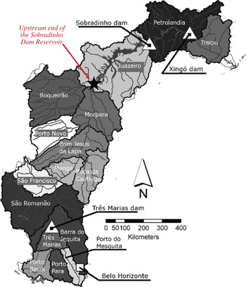
This paper uses a linked hydro-economic model to assess the joint effects of a specific policy change governing minimum flow requirements and one agricultural price shock. Regarding water policy, we simulate a mandatory minimum flow at the upstream end of the Sobradinho reservoir (see figure 1) to maintain storage levels and to meet outflow requirements at the Sobradinho dam set by ANA, the Brazilian National Water Agency. We also simulate a large increase in the price of sugar cane.
Watersheds of the SFRB as defined in the Hydrologic Model

2. The economic model
The economic model of agricultural production detailed below is based on Positive Mathematical Programming (PMP; Howitt, Reference Howitt1995). Some examples of studies that rely on PMP for simulations and policy analysis include Howitt and Gardner (Reference Howitt and Gardner1986), House (Reference House1987), Kasnakoglu and Bauer (Reference Kasnakoglu, Bauer, Bauer and Henrichsmeyer1988), Arfini and Paris (Reference Arfini, Paris and Sotte1995), Chatterjee et al. (Reference Chatterjee, Howitt and Sexton1998), Lance and Miller (Reference Lance and Miller1998), Paris and Howitt (Reference Paris and Howitt1998), Heckelei and Britz (Reference Heckelei and Britz2000), Preckel et al. (Reference Preckel, Harrington and Dubman2002), Röhm and Dabbert (Reference Röhm and Dabbert2003), Cai and Wang (Reference Cai and Wang2006), Marques et al. (Reference Marques, Lund, Leu and Jenkins2006), Cai et al. (Reference Cai, Ringler and You2008) and Maneta et al. (Reference Maneta, Torres, Wallender, Howitt, Vosti, Rodrigues and Bassoi2009a).
Farmers in a given município within the SFRB chose input quantities X that maximize net revenue (net) from I cropping and livestock activities in a base year. That is:

where X i is an h × 1 vector of input quantities used in crop i, p i is the price per ton of perennial and annual crops and of the outputs associated with livestock activity, produced according to a production function q i(X i, P i).Footnote 5 Inputs include: land (land), surface water used for irrigation (sw), hired labor (lb), family labor (flabor), and the quantities of other materials (mat) used to produce crop i – these are labeled, respectively, as X iland}, X isw, X ilabor, X iflabor, X imat.Footnote 6 We distinguish inputs that are used for irrigated production and inputs used for rainfed production by superscripts on X: ir for inputs used in irrigated crops, and r for inputs used in rainfed crops. For example, the quantity of land used in irrigated crops is denoted as X ilandir, and in rainfed crops, X ilandr. We omit the superscript in the case of applied water since it only appears in the production process of irrigated crops. P i represents the amount of precipitation that falls onto the land area covered by the i th crop during its growing season; precipitation contributes to livestock via pasture productivity.
Production costs are defined by the last two terms in equation (1): the first term is the sum of market prices of the inputs, p h, multiplied by the quantity of inputs used in production, X ih. The second term, in parentheses, has a quadratic specification, with parameters αi and ψi, and takes into account the implicit increasing (unobserved) costs associated with allocating land to the i th cropping or livestock activity (X iland).Footnote 7
2.1. Production functions for rainfed and irrigated crops
Based on the constant elasticity of substitution (CES) functional form, production functions are modeled separately for rainfed and irrigation conditions. If a crop is exclusively rainfed (r), i.e., no irrigation technology is in place and hence surface water is not used as an input, then production is modeled as:

where A i, b iland, b iflabor, b ilabor and b imat (for land, family labor, hired labor and materials, respectively) are crop-specific production function parameters. γ = (σ − 1)/σ, where σ is the elasticity of input substitution and ɛi is the returns-to-scale parameter. Precip i = P ia/P ie, where P ie is the expected level of precipitation based on long-term weather patterns, and P ia is the actual level of precipitation in the year for which production functions are estimated.
If a crop can be irrigated (ir), production is modeled as:

where A i, b iland, b iflabor, b ilabor, b imat, γ and ɛi are defined as in (2); b iw is the crop-specific production function parameter associated with water use from two sources: surface water irrigation (X isw) and/or actual precipitation (P ia).Footnote 8
2.2. Production function parameter values
The production function parameters are analytically calculated using profit maximization first order conditions for each input (value of the marginal product of each input equalized to its unit cost). For unconstrained inputs, unit costs are defined as their market prices. Land, family labor and surface water, however, may be non-marketed and of limited supply, and hence may have positive shadow prices. The unit cost of these inputs is then the sum of market prices (if such prices exist for land and water) and their shadow prices. The price of land has a third, crop-specific component related to the amount of land dedicated to a particular crop. It is the value of the LaGrange multiplier associated with a calibration constraint and represents the opportunity cost of allocating land from the least profitable to a more profitable crop.Footnote 9
Along with these first order conditions and assuming constant returns to scale for all crops (ɛi = ɛ = 1), a value of 0.4 for the elasticity of substitution (σ), and Precip i = 1 in (2),Footnote 10 each of the parameters b ih, A i, αi and ψi in equations (1), (2) and (3) can be expressed as a function of input prices, output prices, input quantities and shadow values.Footnote 11
2.3. Economic simulation model
Using the calibrated CES production functions for rainfed and irrigated crops, and the parameterized implicit cost of land in (1), we derive the objective function for the maximization problem for each município (n) in watershed c (subscripts n and c omitted for clarity) in a given year:

where according to equations (2) and (3),  and
 and
 are the calculated parameters.Footnote 12
This maximization problem is restricted by a set of linear constraints on the annual amounts of land and family labor, and on the monthly amount of surface water, available in each município.Footnote 13 It is assumed that in each município, the annual amount of water intended for use on a given crop is distributed monthly according to the crop evapotranspiration needs. For example, if soybeans in a given município are planted in January and harvested in April, and if out of the total evapotranspiration occurring over this cropping period 15 per cent occurs in January, 25 per cent in February, 40 per cent in March, and 20 per cent in April, then the annual water intended for use in soybean production must be allocated monthly according to these percentages. For each crop (i) these monthly percentages are embodied in a matrix called Met im (monthly evapotranspiration).
Formally, the set of constraints are represented by the following equations:


where X iland, X iflabor and X isw m in equation (5) are, respectively, the amounts of land, family labor, and surface water used in the production of crop i or in maintaining pastures for livestock. Notice that while the time steps for land and family labor are annual, for surface water it is monthly (hence the subscript m). B land, B flabor and B sw m are the total amounts of each input available for use at their respective time steps.Footnote 14 Equation (6) sets up the rule for the monthly distribution of the annual amount of surface water that a município intends to use to irrigate crop i (X isw). See section 5 for a description of the steps taken in the construction of Met im.
Predicted results from this optimization run in terms of crop and input mix were then compared against the baseline values. Considering all inputs, municípios and crops, 95 percent of the differences between an input quantity the model predicts and its baseline year value were within an acceptable range between −1 per cent and 1 per cent. Therefore the economic model was considered as calibrated and suitable for simulation purposes.
3. The hydrologic model
The hydrologic model is based on a semi-distributed modeling and water accounting approach implemented in MIKE Basin (Danish Hydraulic Institute, 2005). In this model, the basin is characterized as a network of interconnected elements (catchments, channels, water users or reservoirs) that can store, transfer or use water. A mass balance equation is solved for each of these elements, and time step dictated by the inflow and outflow information provided by the water use agencies. For each catchment, the main water inputs included in the model are rainfall and incoming flow volume from the adjacent catchments located upstream.
The main outputs of the model are flows out of the catchment and evapotranspiration volumes. The flows out of the catchment are calculated as the sum of the inflows from the upstream catchment, plus the flows generated inside the catchment minus water extractions by users. The flow generated inside a given catchment is calculated by subtracting the discharge records of the upstream neighboring catchments from the recorded outflows of the given catchment. The outflow in turn becomes an input either into the adjacent downstream catchment or a reservoir (if there is one associated with the given catchment). In catchments where a reservoir exists, a storage-release function is provided so the actual outflow out of the catchment is modulated by the reservoir based on its storage capacity and the water release policy. The water accounting in the reservoir is kept by adding water inflows and subtracting water releases. For catchments associated with water users, the prescribed water needs of these users are subtracted from the flows out of the catchment or storage in reservoirs, plus 10 per cent estimated losses in the water conveyance and irrigation channel systems.
The water needs (or demand) in watershed c in month m are calculated assuming that farmers in the municípios fully satisfy the plant water needs that are not met by rainfall. More specifically, from equation (6) the hydrologic model knows that the water used in município n located in watershed c in month m is (∑iX isw m)nc. Therefore, the total water demand in watershed c in month m is

where N is the number of municípios in watershed c.
With discharge records from 16 stations, the SFRB is divided in 16 sub-catchments, four of which contain reservoirs. Figure 1 depicts the SFRB and the 16 watersheds contained in the model. Water stocks and demand by the water users (see section 5) in the SFRB were simulated stochastically using 16 multi-normal probability density functions for monthly rainfall, potential evapotranspiration and discharge derived from recorded data for each sub-catchment. Two thousand Monte-Carlo simulations were run for the baseline scenario and for the scenario with increased irrigation to obtain the frequency distribution of river flows and storages in reservoirs.Footnote 15
4. Hydrologic and economic models: linkages
Because water stocks and demands in the SFRB are simulated stochastically using the rainfall, evapotranspiration and discharge probability distribution functions derived from recorded data, it is possible to evaluate the economic model using water availability constraints with a given probability. That is, for each month (m), there is a given amount of surface water (B sw m)c associated with a probability p (as obtained from the water stock probability distribution function derived from the Monte Carlo simulations) that can be used by the municípios in watershed c to irrigate their I crops. The amount of water available to município n, located in watershed c, in month m, is then calculated as

where σn is the percentage of total irrigated area in watershed c that is in município n.Footnote 16 Notice that (B sw m)nc in equation (8) is equivalent to B sw m in (5), in which subscripts c and n were omitted for clarity.
More specifically, the hydrological model ‘feeds’ the economic model in equation (5) with an estimate of B sw m for each watershed and their municípios with a desired level of probability (i.e., the probability that the required volume of water is available in the channel at a given month). The economic model incorporates this information into the water constraint and calculates how farmers adjust their input and output mixes. Once the economic model has identified the optimal cropping and pasture activities given the water (and the other) constraints, it is possible to explore the effects of exogenous shocks (such as changes in crop prices) on famers’ decisions given water constraints. Alternatively, the water constraints can be relaxed and farmers may readjust their water use accordingly. The Monte Carlo simulations can then be rerun with the new optimal crop mixes, land allocations, and production technologies to obtain new river flow frequency distributions. These distributions can be used to evaluate the likelihood that under the new set of agriculturally optimal cropping activities, river flows would be depleted below a predetermined rate (e.g., reducing river discharge below an established minimum environmental flow).
5. Data and calculation of water demand for irrigation
For this paper, the hydrological model relies on discharge data from DSS522.1 dataset (DE/FIH/GRDC and UNESCO/IHP, 2001) and on data of precipitation and evapotranspiration at the sub-watershed level from CRU{_}TS{_}2.10 dataset (Mitchell and Jones, Reference Mitchell and Jones2005). The calibration and calculation of the parameters of the economic model uses município-level data on inputs and outputs (quantities and prices) mostly from the Brazilian Agricultural Census1995/1996 (IBGE, 1998).Footnote 17 Due to the unique approach used to build the monthly evapotranspiration percentages matrix Met im and to calculate the annual amount of water used for the calibration of the hydrological and economic models, we detail them in this section (see below).
The database on applied water per crop was built in the following way. A crop calendar divided into the 12 months of the agricultural year provides the most probable dates of planting and harvesting for crop i grown in watershed c. With data on precipitation and atmospheric demand per watershed c, we then calculate the amount of irrigation water applied to the crop by using the formula:

where (W im)c is the amount of applied water on crop i in watershed c in month m for the irrigation of crop i. k i is a technical crop coefficient associated with crop i, ET cim is the potential evapotranspiration in watershed c associated with crop i in month m. Precip cim is the amount of rainfall in watershed c in month m that fell onto the land area covered by the i th crop and IEff is average irrigation efficiency, assumed to be 70 per cent. Data for k i, ET cim and Precip cim come from Allen et al. (Reference Allen, Pereira, Raes and Smith1998) and Mitchell and Jones (Reference Mitchell and Jones2005). The max function ensures that if in a given month Precip cim > k i · ET cim, the numerator becomes negative and thus(W im)c is assumed to be zero. The annual amount of water used in a given município n, located in watershed c, on the irrigation of crop i, (X isw)nc is calculated as

where νin is the percentage of the total irrigated area allocated to crop i in watershed c that is in município n. Notice that (X isw)nc in equation (10) and X isw in (6) are equivalents. We just omitted subscripts n and c from (6) for clarity.
The Met im is constructed based on the notion behind (9). For all municípios that belong to watershed c and for the months in this watershed in which Precip cim < k i · ET cim, we create a variable Z cim = (k i* ET cim) − Precipcim, Z cim = 0, otherwise). In this manner, the annual agronomically optimal evapotranspiration is  . Met im is then defined as the ratio between the monthly and annual agronomically optimal evapotranspiration when supplemental irrigation is necessary, that is,

in which subscripts n and c were omitted for clarity.
6. Simulations and results
In this paper we examine the impacts of minimum flow regulations and of an exogenous price shock on the agricultural activities, incomes and employment in 59 municípios located within two contiguous watersheds located in the north-central part of the SFRB: Boqueirão which is located upstream and Juazeiro which is located downstream (see figure 1). The area encompassed by these two watersheds includes the Sobradinho reservoir and dam, and has experienced (although not spatially uniformly) above-average increases in area dedicated to diversified commercial agriculture over the past 10 years vis-à-vis the rest of the SFRB. The Boqueirão watershed includes the município of Barreiras which is home to large-scale grain (especially soybeans) producers who practice irrigated agriculture using center-pivot technology. The other downstream watershed (Juazeiro) includes part of the municípios of Petrolina and Juazeiro, which have several irrigation districts within which highly diversified, small- and medium-scale agricultural systems produce a broad array of tropical fruits and grapes.
These two watersheds differ in terms of crop mix and scale of operation. Although both watersheds contain some large-scale farms (defined here as comprising more than 500 ha), these represent just 43 per cent of all farms in Juazeiro but approximately 81 per cent of all farms in Boqueirão. Small-scale farms (defined here as comprising up to 20 ha) are essentially absent in Boqueirão, while in Juazeiro they represent up to 12 per cent of all farms. So, in general, Boqueirão's agriculture is based on large-scale operations while in Juazeiro farm size distribution is more even, with a significant percentage of small- and medium-scale operations. It also tends to be more parsimonious with the use of inputs compared to Juazeiro. In fact Boqueirão consistently tends, on a per hectare basis, either to use lower quantities of inputs or to expend less with them overall.Footnote 18
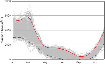
Regarding water use regulations, ANA, the Brazilian agency for water resources, currently stipulates 1,815 m3/s as the minimum outflow flow from the Sobradinho Dam (see figure 1). Our Monte Carlo simulations, based on historical data on discharge (DE/FIH/GRDC and UNESCO/IHP, 2001) reveal, however, that under drought conditions it would be difficult to meet this outflow and maintain the reservoir at a constant level. We therefore simulate the effects on the agriculture in the two sub-catchments (Boqueirão and Juazeiro) of the effective implementation of the ANA mandatory regulation on the inflows at the entrance to the Sobradinho reservoir (see the star in figure 1) by stipulating a minimum inflow of 2,000 m3/s during all months of the year. Figure 2 depicts continuous water availability at the entrance to the dam ‘net’ of the 2,000 m3/s required by law. The cluster of grey curves reports the simulated flows under different weather conditions; all flows at or above the solid upper line represent the 5 per cent very wettest years, while those at or below the dashed line represent the 5 per cent very driest years. The reader will note that during the seasonally dry months (e.g., July through October) very little water is available for agriculture once the ANA in-stream flow requirements have been met.
Baseline water availability at the entrance to Sobradinho Reservoir as calculated by the set of Monte Carlo simulations

We also simulate an increase in the price of sugar cane, a commodity grown throughout the SFRB. Brazil has been experiencing a boom in sugar cane production due to high domestic and international prices, and steady increases in domestic and international demand for ethanol. In fact, sugar cane area has increased 23 per cent and production 32 per cent over the past 10 years (IBGE, 2000–2009). In this context, we simulate the effects of even higher demand for sugar cane/ethanol represented by a five-fold increase in the price/ton.Footnote 19
In these simulations we assume that municípios upstream of Boqueirão are not affected by the price policy and that they will behave as they have behaved historically in terms of their farming practices under the dry and wet conditions. Excluding municípios that are upstream provides, therefore, an estimate of the minimum effects of the price shock on water supply (and on income/employment) on Juazeiro and Boqueirão.
6.1. Scenarios
The minimum flow requirements and the increase in prices are simulated under two scenarios derived from the flows depicted in figure 2, one optimistic and one pessimistic. Under the optimistic scenario, surface water available for agriculture in each month is the average of flows in a given month based on the 5 per cent wettest years, again, after the ANA-mandated 2,000 m3/s is deducted. Under the pessimistic scenario, this average is calculated based on the 5 per cent driest years. We also assume that official rules guarantee agriculturalists at least 10 m3s−1 of water for irrigation regardless of weather conditions or month of the year.Footnote 20
6.2. Effects on area, agricultural employment, farm profits and input-output mix
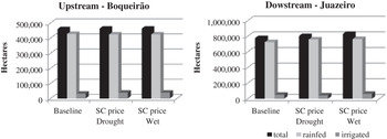
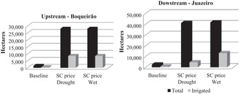
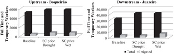
While the ANA regulation on water use per se would not be binding for agriculture in both watersheds under baseline year and average weather conditions, figures 3–6 show a different picture when a drought and increased sugar cane prices are added to the simulation. These figures report baseline land use, area dedicated to sugar cane, agricultural employment and farm profits, and the effects of the sugar price increase on these agricultural outcomes under different extreme weather scenarios. Note that SC in the figures refers to sugar cane.
Hectares of total cultivated land, upstream and downstream, by weather (drought or wet) and five-fold sugar cane (SC) price increase scenarios

Hectares of cultivated land dedicated to sugar cane, upstream and downstream, by weather (drought or wet) and five-fold sugar cane (SC) price increase scenarios

Number of workers employed, total and irrigated agriculture, upstream and downstream, by weather (drought or wet) and five-fold sugar cane (SC) price increase scenarios

Agricultural profits, upstream and downstream, by weather (drought or wet) and five-fold sugar cane (SC) price increase scenarios

In both upstream and downstream areas, rainfed agriculture dominates the landscape prior to the increase in sugar cane prices, and continues to do so after the price increase (see figure 3). That said, the total area under cultivation increases in response to the price increase, slightly in the upstream and more significantly in the downstream areas, and proportional increases in the number of hectares dedicated to irrigated agriculture are larger than those for rainfed agriculture in both areas. Finally, cultivated area is not particularly influenced by the extreme weather patterns included in this set of simulations.
The area dedicated to sugar cane, however, increases substantially in both the upstream and downstream areas as a result of the price increase, with the largest absolute increases in both areas occurring in rainfed production (figure 4).Footnote 21 Extreme weather does not seem to influence upstream sugar cane production, but the same is not true for the downstream area which has to dramatically reduce irrigated sugar cane cultivation during the dry year due to a lack of available water for irrigation.
Figure 5 depicts the effects of the five-fold price increase on agricultural employment, under wet and dry weather scenarios. Employment gains associated with the price increase are small, primarily because the proportion of agriculture dedicated to sugar cane before and after the shock is not large.Footnote 22 In addition, sugar cane production is not particularly labor intensive, except during harvest. Likewise, the effects of water use regulations and drought also do not affect the employment pattern greatly when we look at agriculture as a whole (i.e., rainfed and irrigated agriculture). This is expected given the dominance of rainfed agriculture on employment before and after the price and weather shocks. However, if we focus on irrigated agriculture, it is clear that employment could be reduced by as much as half in the event of a drought vis-à-vis a wet year in Juazeiro.
Finally, the large increase in sugar cane prices has a large, positive effect on farm profits in both the upstream and downstream areas, and under both extreme weather scenarios (figure 6). However, downstream farmers are forced to reduce irrigated sugar cane production (and other forms of irrigated agriculture) during the dry year, and their profits suffer as a consequence. The same is not true for upstream farmers who have ‘first claim’ to surface water, which they use at the expense of downstream farmers during a dry year.
All in all, these results show that the effects on agriculture of regionally uniform policies and external shocks will not be spatially uniform. Under the ANA-mandated river flow regulations, farmers’ production possibilities will be greatly influenced in Juazeiro, the downstream watershed, relative to those of upstream farmers in Boqueirão, in the event of a region-wide drought and an increase in sugar cane prices. Boqueirão has the ‘right by position’ to withdraw water first and as a consequence will never face a water binding situation under the regulation, even when sugar cane prices and associated water demands increase. On the other hand, Juazeiro's inflows are Boqueirão's outflows, so its farmers face increased water scarcity during the dry season, in dry years.
The equity effects of the price shocks will also tend to differ regionally, especially during drought years. In Boqueirão, large-scale farms dominate the landscape, while in Juazeiro there are many small- and medium-scale farms. While the data do not allow us to precisely estimate the effects of price increases or weather shocks on different scales of agricultural operations, the strong and negative effects of a drought on downstream Juazeiro suggest that small- and medium-scale farmers and their employees would be hit harder since they happen to be located in this downstream watershed.Footnote 23 Also, although farmers can adjust to changes in input scarcity (e.g., by investing in improved seeds, producing more high-value crops or increasing irrigation efficiency), small-scale farmers tend to have fewer such options than large-scale operations to compensate for reductions in agricultural revenues attributable to water scarcity (brought about by drought, policy fiat or both). Hence, the regulations imposed by ANA can, ceteris-paribus, cause hardships that fall disproportionately on small-scale agriculturalists.
Lastly, a final round of simulations is performed to shed some new light on the debate over two agricultural and natural resources topics: biofuel policies and water market trading potential. In the case of biofuel policies, we examine the effects of the five-fold price increase on the use of water, pesticides and fertilizers, and on the reallocation of land to alternative cropping activities. Weather and river flow conditions in the baseline year are used as a basis for these simulations. In Juazeiro, the increase in sugar cane area would be mostly at the expense of fruits and vegetables such as mango, melons and tomatoes, and staple crops such as rice. In Boqueirão, the increase would also be at the expense of fruits and vegetables such as citrus, mango and bananas, and staple crops such as beans and manioc. Regarding hydrologic effects, water use in agriculture (via irrigation and increased evapotranspiration) in Juazeiro would increase by 329 million m3 (or by 211 per cent); in Boqueirão, water use would increase by 129 million m3 (or by 117 per cent). Expenditures on pesticides would increase by R$ 8.5 million (or by 315 per cent) in Juazeiro and by R$ 370,000 (or by 2 per cent) in Boqueirão; expenditures on fertilizers would increase by R$ 12 million (or by 282 per cent) in Juazeiro and by R$836,000 (or by 2 per cent) in Boqueirão.Footnote 24
The water market potential was tested by allowing costless trade between monthly regional surface water rights. More specifically, under the ideal and zero transaction costs market model simulation, a monthly interregional water market improved the objective function value by 26 per cent. In addition, surface water had a scarcity value in June and October in three municípios and in all of them in August. Under a monthly interregional market situation, the shadow value of water, in Brazilian Reais per cubic meter, dropped from as high as 23 in some regions to a uniform 0.435 in August and zero in all other months. We would expect slightly different results under non-zero transaction cost assumptions.
7. Conclusions and policy implications
This paper uses a linked hydro-economic model to explore, in the context of two large watersheds within the SFRB, the effects of the implementation of the Brazilian water use regulations and (simultaneously) a large rise in the price of sugar cane. The application of water use regulations has the expected effect of reducing the surface water flows available to agriculture for irrigation, in all areas. More specifically, in the watersheds examined in this study, a minimum flow requirement at the entrance of Sobradinho Dam of 2,000 m3s−1 reduces the amount of water available for agriculture, in particular in Juazeiro, the downstream watershed. This policy-mandated maintenance of water flows in the SFRB system constrains downstream farmers’ cropping options, especially during dry years.
However, the economic, rural employment and other consequences of minimum flow regulations will depend on (among other things) the product mix and irrigation technologies in place when the regulations are implemented, the location of agricultural activities, weather conditions and input and product prices. More specifically, the linked hydro-economic models show that the site-specific and farm type-specific effects of the application of water use regulations are not likely to be spatially uniform.
The linked hydro-economic models also provide insights into the effects of a large increase in sugar cane prices. Upstream and downstream farmers react (as expected) to the price increase by increasing the area dedicated to rainfed and irrigated sugar cane production, and agricultural profits increase substantially. However, during dry years, downstream farmers do not have access to sufficient water to retain as much area in irrigated sugar cane as they would have liked, so profits fall; upstream farmers, having ‘first claim’ to surface water for irrigation, are able to retain larger areas in sugar cane even during dry years, and hence do not suffer lower profits during drought periods.
The effects of the price shock and the implementation of water use regulations on rural employment are not large. This is due in particular to the dominance of rainfed agriculture on employment, the resilience of employment under drought conditions, the small proportion of total agricultural land dedicated to sugar cane before and after the shocks, and the low intensity of labor use in sugar cane. Although this may imply that effects of these shocks on regional rural poverty will not be large, there may be areas within each watershed with proportionally larger areas dedicated to irrigated agriculture that do suffer large, negative employment effects, particularly in the downstream areas during dry years. The encouraging news is that the expansion of the sugar cane area associated with the price shock does not ‘crowd out’ the other irrigated crops (e.g., fresh fruits and vegetables) that small-scale agriculturalists and rural laborers are most likely to participate in and benefit from. The increase in area dedicated to sugar cane would, however, be at the expense of some staple crops such as rice, dried beans and manioc, with some implications for local product prices for these commodities. Although preliminary, these results do suggest that there may be important environmental and food security implications associated with policies aimed at increasing biofuel production based on ethanol in the area of study.
Finally, the simulations also show that a hypothetical trading of monthly water rights, under zero transaction costs, would alter the model results under the drought and price policy scenarios. In fact it would cause a positive change in social returns, measured by the value of the objective function, and lower the surface water scarcity values. That being said, it is important to note that the establishment of tradable monthly water rights has not yet been implemented in Brazil so the concept of trade in monthly water rights is currently not a practical alternative, but should be studied in the future.
Supplementary material
The Supplementary material referred to in this article can be found online at journals.cambridge.org/EDE.