1. Introduction
What factors increase or decrease the probability that an event occurs? The question is a familiar one in political science. Wars, votes, reelection, policy adoption, democratic reversals, and treaty formation are some examples of events whose occurrence we have an interest in understanding. Yet for many of the events we study, it is reasonable to suspect a subject’s likelihood of experiencing the event is, at least in part, dependent upon how long the subject has been at risk. This suggests events exhibit duration dependence: the probability of an event occurring in time period j depends on t, the amount of time elapsed since the subject could first experience the event.
Because of concerns about duration dependence, both as a so-called statistical nuisance and potentially a theoretically meaningful concept, methodologists have spent time discussing various corrections for such dependence. The most widely utilized correction at present comes from Beck, Katz, and Tucker (Reference Beck, Katz and Tucker1998; hereafter “BKT”), who suggest using logit or probit models (henceforth L/P) with time trends for binary outcomes exhibiting duration dependence, implicitly treating time as a discrete phenomenon. The time trends account for the duration dependence, removing a possible source of omitted variable bias in the L/P context (Mood Reference Mood2010).
We argue researchers working with binary time-series cross-sectional (BTSCS) data should consider using Cox semiparametric duration models in place of L/P. While L/P models with time trends and Cox models are very similar, we contend that accounting for duration dependence via Cox models presents several unique advantages. We demonstrate that Cox models are generally adept at correctly modeling data-generating processes (DGPs) characterizing typical political science BTSCS data, even though such data split time into discrete intervals (e.g., years, months, etc.)—a potential challenge for Cox models, which assume time is continuous. We use Monte Carlo simulations to bring new evidence to light showing Cox models perform just as well—and sometimes better—than logit models in a basic BTSCS setting, from a bias and efficiency standpoint. Additionally, we show the Cox outperforms L/P in more complex BTSCS situations involving distinctions between event onset and event duration (McGrath Reference McGrath2015), as well as situations where covariate effects are potentially conditional on time and/or a process’ current state—the first time that Cox versus L/P have been evaluated in such a way.
In addition, we offer three principal substantive reasons to consider using Cox models. First, semiparametric duration models force scholars to be more cognizant of the proportional hazards (PHs) assumption, which can cause biased coefficient estimates and standard errors if left uncorrected. Second, semiparametric duration models are a gateway to modeling more complex processes. As a common example, many studies’ datasets fail to differentiate between the onset of an event and the duration of an event, yielding potentially biased estimates (McGrath Reference McGrath2015, 534–535). Finally, semiparametric models eliminate possible bias from misspecifying the event’s baseline hazard, which denotes the underlying risk of the event’s occurrence over time. Baseline hazard misspecification can lead to inefficiency at best, and biased covariate effects and predicted quantities at worst (Box-Steffensmeier and Jones Reference Box-Steffensmeier and Jones2004, 21–22).
Despite the Cox model’s potential virtues for BTSCS data, potential barriers to its use remain. One common ancillary complaint is the Cox’s dearth of easy-to-interpret postestimation quantities, leading some to prefer L/P. To address these secondary concerns, we advocate for using transition probabilities for interpreting duration models, as they are more intuitive quantities for readers to engage with. We discuss how to estimate and interpret these transition probabilities in online Appendix B and in other work (Jones and Metzger Reference Jones and Metzger2019).
The paper proceeds in five parts. First, we discuss current approaches to modeling BTSCS data. We also summarize our Monte Carlo simulations assessing the Cox model’s performance versus logit in standard BTSCS settings. Second, we elaborate on three potentially significant issues stemming from BTSCS data that Cox models handle more elegantly than L/P. Third, we assess the relative performance of Cox and L/P models in addressing these three issues via Monte Carlo simulations. Fourth, we provide an example BTSCS application, originally estimated using a logit model, to highlight the potential difficulties of L/P in the BTSCS context, and how Cox models provide an accessible alternative. Our fifth and final section concludes.
2. Modeling BTSCS Data: Current Approaches
A large swath of political science research examines whether an event occurs, making the dependent variable binary. We often have time-series cross-sectional data on multiple panels, with each subject i’s panel composed of observations from multiple points in time (j, to denote calendar time). Data of this form are BTSCS data, which are also grouped duration data (BKT Reference Beck, Katz and Tucker1998). L/P models are standard tools for evaluating hypotheses about an event’s occurrence.
For many of the events we study, it is reasonable to suspect temporal dependence exists: whether a subject experiences the event in the current time period j is dependent upon how long the subject has been at risk of experiencing the event. This length of time is t, our duration.Footnote 1 By default, L/P both assume temporal independence. No covariate captures t’s effect on the probability of the event occurring in j. BKT (Reference Beck, Katz and Tucker1998) point out the importance of accounting for temporal dependence, because failing to do so amounts to assuming an incorrect functional form for the baseline hazard (h 0(t)). A wrong h 0(t) functional form in BTSCS models has the same ramifications as it does for parametric duration models: inefficiency at best, and biased estimates and predicted quantities at worst (BKT Reference Beck, Katz and Tucker1998, 1261; Box-Steffensmeier and Jones Reference Box-Steffensmeier and Jones2004, 21).
Numerous strategies exist to correct for temporal dependence, but perhaps the most common correction is to include cubic polynomials as regressors (t, t 2, and t 3)Footnote 2 because of how easily they are generated and their flexibility in capturing many different forms of temporal dependence (Carter and Signorino Reference Carter and Signorino2010). An alternative from BKT is to include splines of time as a regressor to capture the potential nonlinearity of t’s effect.
L/P are not the only models capable of addressing temporal dependence in BTSCS data. BKT (Reference Beck, Katz and Tucker1998, Appendix), among others, show a BTSCS complementary log–log (cloglog) model with time dummies is identical to a (continuous-time) Cox model.Footnote 3 The clear implication is that Cox models can also be used for modeling BTSCS data. However, while we know about the mathematical equivalence of a Cox and a cloglog with time dummies, the two models make different assumptions about time. The latter implies a discrete-time process, whereas the Cox assumes a continuous-time process.Footnote 4 The continuous versus discrete distinction is relevant, because we do not know with certainty whether the Cox/cloglog equivalence holds when it comes to the estimators’ performance under various conditions.
As a preliminary step, we simulate 54 different basic Monte Carlo scenarios to assess the performance of Cox models compared to logit models with cubic polynomials and logit models with natural cubic splines.Footnote 5 We consider true continuous-time durations, continuous-time durations coerced into a start–stop format,Footnote 6 and true discrete-time durations. Within each of these DGP classes, we vary the baseline hazards and sample sizes, but otherwise, the scenarios contain no assumption violations.
The results of these preliminary simulations largely confirm that what we know in theory about the relationship between the Cox and logit bears out in practice. Both the Cox and logit recover unbiased estimates of a covariate’s true effect. As a slight wrinkle, our simulations show the Cox performs better across the board with less biased estimates of βx , and that this improvement is of sufficient magnitude to offset the Cox’s larger standard errors, resulting in a smaller root-mean-squared error (RMSE). Even the simulations from the truly discrete DGPs, which ought to favor logit, tell the same story, by and large. The takeaway from these simulations is simple: Cox models typically perform as well, if not better than L/P, offering a strong rationale for researchers to employ them when modeling most BTSCS data (aside from the situations described in online Appendixes G.A.3 and I).
3. Current Practice: Limitations of Logit/Probit for Modeling BTSCS Data
There are at least three additional complexities associated with BTSCS data that further advantage the Cox model but have received insufficient attention. While L/P are capable of addressing these points from a technical perspective, the models can run into estimation issues, in practice. Cox models can address our three points more easily, relatively speaking.Footnote 7
3.1. Proportional Hazard Assumption
First, and most important in the majority of applied work, is the assumption regarding proportional hazards (PHs). The PH assumption says any covariate’s effect on an event’s risk of occurring is proportional over time. If the PH assumption is met, for instance, an event five times more likely to happen when x = 1 versus x = 0 at time 1 will also be five times more likely to happen when x = 1 versus x = 0 at every other time point. While this assumption is most closely associated with the Cox model, logit models also make an equivalent proportionality assumption—we assume x’s effect is unconditional on time.Footnote 8
PH violations in L/P have the same effects as they do in a Cox model. The issue is identical to the standard interaction term situation: x’s effect is of interest, but x’s effect is conditional on some z, and failing to account for the conditionality may yield misleading estimates of x’s effect. Such violations introduce a form of model misspecification, potentially biasing estimates of both coefficients and standard errors for some or all of the covariates in a model. Thus, not identifying and correcting PH violations is problematic, because even if time is not deemed to be theoretically meaningful, failing to account for its conditioning effects can nevertheless bias a model’s results. L/P models in a BTSCS context are not exempt—here, too, we should be testing for PH violations, a point Carter and Signorino (Reference Carter and Signorino2010, 289) make readily.
However, in practice, testing for PH assumption violations with L/P is cumbersome. The test requires estimating a likelihood-ratio test using the core restricted model and an unrestricted model that includes an interaction between the time polynomials and a covariate. This procedure must then be repeated for each covariate in the model (Carter and Signorino Reference Carter and Signorino2010, 289). As a result, practitioners may not consistently follow Carter and Signorino’s (Reference Carter and Signorino2010) advice to test for PH violations in L/P models. By contrast, testing for PH violations after a Cox model is trivial, as canned routines exist in standard software packages.
To see whether practitioners check for PH violations in L/P contexts, we used Google Scholar to identify all articles citing Carter and Signorino (Reference Carter and Signorino2010) published in the American Political Science Review, the American Journal of Political Science, and the Journal of Politics between 2010 and 2016. From this sample, we examined the 26 articles reporting at least one L/P model with cubic polynomials in the main text. We checked to see whether each article reports any PH violation tests for the L/P model(s) with cubic polynomials, and/or whether the article’s reported models include any corrections for PH violations. Surprisingly, we find only 1 of the 26 articles (3.9%) explicitly mentions testing for PH violations or implements corrections for violating this assumption. In comparison, Jin and Boehmke (Reference Jin and Boehmke2017, 142) find that in a sample of 43 studies using Cox models, 31 (72.1%) report testing for PH violations.
Moreover, we replicate the first L/P model with time polynomials reported in each paper from our sample, re-estimate it as a Cox model, and perform standard tests of the PH assumption.Footnote 9 Regardless of how the PH test is specified, we find evidence of PH violations in at least half of these models, and potentially many more. Focusing solely on the coefficients within these models, our evidence suggests nearly a third of them may exhibit nonproportionality. Given the potential for model misspecification and erroneous inferences arising from PH violations, not testing for these violations is quite troubling.
3.2. Causal Complexity
Second, Cox models can easily handle causally complex processes in which “the effect of one variable or characteristic…depend[s] on which others are present” (Jervis Reference Jervis1997, 35). Arguments involving causally complex processes in political science “are both common and prominent” (Braumoeller Reference Braumoeller2003, 209). Examples range from a basic two-variable interaction via an interaction term, to the identification of heterogeneous treatment effects across subsamples (Athey and Imbens Reference Athey and Imbens2016; Grimmer, Messing, and Westwood Reference Grimmer, Messing and Westwood2017), to a variable’s effect differing from the onset to duration of an event (McGrath Reference McGrath2015), which we explore in more detail below. Researchers’ model specifications must acknowledge the conditionality implied by causal complexity; otherwise, misspecification bias will result.
Cox models can also accommodate causal complexity. Jones and Branton (Reference Jones and Branton2005) emphasize the similarity between BTSCS setups and Cox models, noting the Cox model’s ability to handle additional process structures that L/P struggle with—namely, competing and repeated events.Footnote 10 Metzger and Jones (Reference Metzger and Jones2016) extend Jones and Branton’s list, showing that Cox models can also handle additional process structures (e.g., recursiveness and sequential events) when formulated as a multistate model. They further discuss how multistate models can account for the determinants of transitions between these stages, with the ability to specify transition-specific covariate effects without using conventional interactions. Metzger and Jones (Reference Metzger and Jones2016) also subsequently show the importance of modeling all the process’ stages, to protect against inaccurate and misleading inferences about x’s effect. In short, using Cox models in a BTSCS setting can more readily give researchers additional modeling freedom than L/P currently offers, giving us more leverage to test additional implications from our theories.
One particular form of causal complexity in BTSCS settings relates to properly defining the outcome of interest. As McGrath (Reference McGrath2015, 534–535) describes, many studies’ datasets fail to differentiate between the onset of an event and the subsequent duration of an event, with 65% of studies in McGrath’s meta-analysis miscoding ongoing events. To provide a concrete example using our application: consider a militarized interstate dispute (MID) that commences in 2000 and terminates in 2003. Common practice is to code years in which MIDs are ongoing as 0. In this case, 2000 would be coded as 1, and 2001, 2002, and 2003 would be coded as 0. By doing so, researchers introduce a situation of heterogeneous 0s, where 0 either indicates peace or an ongoing conflict. McGrath shows estimates of x’s effect on onset will be biased as a result (McGrath Reference McGrath2015, 536–538). The same principle holds if the dependent variable is coded as 1 in 2000 and each of the intervening years through 2003. We potentially introduce heterogeneity for the 1s, in turn concealing any different covariate effects for onset versus duration (McGrath Reference McGrath2015).
3.3. Baseline Hazard
Finally, using semiparametric models removes a possible source of bias stemming from misspecifying the baseline hazard’s functional form. Misspecification can arise in L/P because these models explicitly parameterize the baseline hazard during estimation, often using a cubic polynomial. When we do this, we are saying our baseline hazard’s functional form is a cubic polynomial of time—that the baseline hazard of our event’s occurrence when all other covariates are equal to 0 is of the form t + t 2 + t 3.
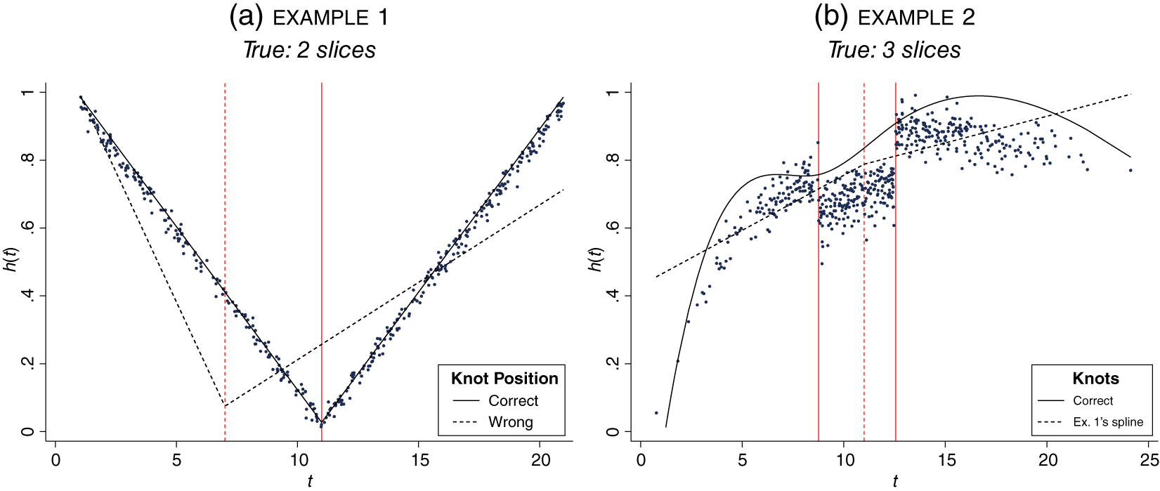
We could also model the baseline hazard using splines (BKT Reference Beck, Katz and Tucker1998), as their flexibility means they may be less prone to imposing an incorrect functional form. The flexibility comes from splines’ piecewise logic, which allows h 0(t)’s functional form to vary across different slices of t values. The boundaries between slices are known as “knots” (Figure 1’s vertical lines). Among other things, practitioners must decide how many knots to use and their location. Due to all these fit-related decisions, correctly implementing splines may be challenging. Carter and Signorino (Reference Carter and Signorino2010, 281–282), for instance, note some practitioners take the number and/or location of knots from another application (e.g., Figure 1a) without assessing whether these choices are reasonable for their own application (e.g., Figure 1b’s dashed lines), resulting in misspecification.
Example datasets, splines.

The risk of misspecifying the baseline hazard’s functional form comes up frequently in the context of parametric duration models. Similar to L/P models with a cubic polynomial, parametric duration models make specific functional form assumptions about how the baseline hazard should be parameterized. Parametric models’ use is often discouraged in the duration modeling literature for social science applications, for precisely this reason. As Box-Steffensmeier and Jones (Reference Box-Steffensmeier and Jones2004, 66–67) argue, “the strong theory required to choose a specific [parametric duration model] distribution is almost always lacking.”
Misspecifying the baseline hazard is not a costless act. It can lead to inefficient and/or biased postestimation quantities (Box-Steffensmeier and Jones Reference Box-Steffensmeier and Jones2004, 21–22), because it amounts to using the wrong formulae for any postestimation calculations. Thus, duration modelers in the social sciences are encouraged to use the Cox model if they lack theory-based predictions about the baseline hazard’s functional form.
Crucially, this point from the duration modeling literature is equally valid in an L/P context. If we are concerned with baseline hazard misspecification for parametric duration models, logical consistency demands we also be concerned with the same issue for L/P models with cubic polynomials or splines, because both parametric duration models and L/P explicitly parameterize the baseline hazard. This misspecification occurs regardless of whether we regard time as substantively meaningful or a statistical nuisance, as the baseline hazard’s functional form is intrinsic to the process generating the data. By contrast, using a Cox model avoids these issues entirely, regardless of context, because the Cox does not parameterize the baseline hazard.
4. Complex Processes: Assessing Model Performance
4.1. Key Implications
The three points we raise in the previous section are each valid in their own right, but when taken collectively, give rise to an important corollary: Cox models will typically have fewer issues modeling more complex substantive processes than L/P. As for why, Cox models can model the same process with fewer parameters because, unlike L/P, the Cox does not parameterize the baseline hazard (i.e., it is semiparametric)—a fact that has powerful ripple effects in conjunction with our other two points.Footnote 11
For instance, consider a simple process with a single covariate in which:
-
• There is one stage, equivalent to saying a subject is at risk of experiencing one event. Once the event occurs, the subject is no longer at risk of experiencing any events.
-
• The stage’s baseline hazard is constant across time.
-
• There are no PH violations.
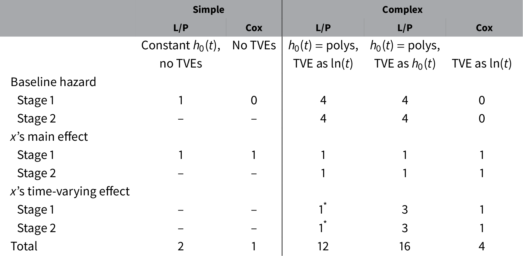
Despite the process’ simplicity, a properly specified L/P will always have more parameters than the Cox (Table 1, first two columns), because L/P estimates a constant term, but the Cox does not. However, L/P only has one additional parameter than the Cox in this context, often leading researchers to disregard the Cox’s semiparametric nature as a compelling reason to use it instead of L/P.
Summary: number of estimated parameters by estimator.

Notes: *assumes ln(t) is not included as constituent term; if included, add one additional estimate per stage for “x’s time-varying effect.” L/P’s constant term is included in “Baseline Hazard” count. “TVE as__ ”: interaction term for PH correction [time-varying effect] generated using __ as t’s functional form. “Polys”: t, t 2, and t 3.
Now consider a more complex scenario more in line with political science phenomena (and our previous section’s three points):
-
• There are two stages (e.g., event onset, then the event’s duration).
-
• Each stage has a distinct baseline hazard involving an unknown functional form of time.
-
• The covariate’s effects differ by stage (perhaps the covariate increases the risk of event onset, but reduces the risk of the event ending).
-
• The covariate is a PH violator for both stages (in ln(t), e.g.).
-
• The covariate’s time-varying effect differs by stage.
For L/P, say we model the baseline hazard using the incumbent correction: t, t 2, and t 3.
The difference in each model’s number of estimated parameters is no longer trivial. Properly modeling this process with L/P involves three-to-four times as many parameter estimates as it would with a Cox (Table 1, last three columns). The nontriviality is exacerbated if we consider more sophisticated ways to model L/P’s baseline hazard. For instance, if researchers model the L/P stage-specific baseline hazard using a basic natural cubic spline with m total knots,Footnote 12 there would be m + 1 parameters for each stage’s baseline hazard (excluding the constant). If we were interacting the PH-violating covariate with the stage’s baseline hazard for L/P (Table 1’s second-from-last column), L/P’s number of parameters would increase at a multiplicative rate compared to the Cox (last column). If we increase the number of included substantive covariates to k, and some of the added covariates are also PH violators, the same multiplicative increase would occur for Table 1’s second-to-last versus last column.Footnote 13
L/P’s greater number of estimated parameters has practical ramifications. For even moderately complex processes like our example above, researchers will need more data to obtain well-behaving estimates of the same parameters with L/P than they would with the Cox. As one example, L/P’s likelihood surface will be poorly behaved in situations where one stage has few observations (e.g., Stage 2) because of the paucity of observations relative to the number of stage-related parameters (e.g., 6–8 for Stage 2 in Table 1’s third and fourth columns), giving rise to estimation problems. Anecdotally, we encountered this issue more than once while running the next subsection’s simulations—the Cox would estimate fine for certain sets of parameter values, but the logit would not.
Because of our interest in assessing logit versus the Cox’s head-to-head performance in complex situations, we ultimately report sets of parameter values for which all our L/P and Cox specifications would estimate. However, acknowledging the estimation issues is important for reasons beyond best practices. Their presence is consistent with our larger point: L/P and Cox models both have the technical capacity to address the three points we mention, but the Cox model’s semiparametric nature makes it better able to do so for a variety of processes.
4.2. Simulations: Cox and Logit Performance, Complex Scenarios
We run a number of Monte Carlo simulations to assess our claims about the Cox versus logit’s performance in the presence of PH assumptions and causal complexity.Footnote 14 Our simulations demonstrate that not only can the Cox more readily accommodate these more complex scenarios that may arise in BTSCS data, but its performance in doing so generally exceeds that of logit.
4.2.1. Setup Details
We consider two broad classes of simulation scenarios in this analysis that differ in the data’s true generating process (DGP). We consider:
-
1. Data in which the true DGP is a continuous-time duration setup,Footnote 15 but coerced into a de facto start–stop duration format. For instance, t = 3.24 would be forced to equal ceil(t) = 4. This class of simulations proxies how we usually work with duration data in political science, as we mentioned in the previous section.
-
2. Data in which the true DGP is discrete. We generate our scenarios using both the logit and complementary log–log (cloglog) link functions. Situations with a truly discrete DGP are rare in political science, but the Cox model assumes the underlying DGP is continuous, making this an important case to check. Notably, Cox models can handle truly discrete data by implementing the exact partial likelihood correction (exactp) for tied data (Box-Steffensmeier and Jones Reference Box-Steffensmeier and Jones2004, 58).Footnote 16
We restrict these simulations to have a sample size (N) equal to 250 and estimate four models: (1) a Cox model with Efron ties; (2) a Cox model with exact partial ties; (3) a logit with time polynomials; and (4) a logit with natural cubic splines.Footnote 17 We also estimate a naïve logit that assumes x has the same effect across transitions and that no time-varying effect exists. This specification mimics current practice in applied work within political science.
To introduce additional complexity into our scenarios, we add two features. First, we introduce a relatively straightforward form of causal complexity by specifying that subjects, upon experiencing an event (Transition 1), are then at risk of a subsequent transition back to their initial stage (Transition 2). This structure is akin to studies of the onset and duration of some event, like a war or period of democratic backsliding. Across a range of simulations, we vary (1) the true effect of a covariate, x, for the two transitions, as well as (2) the baseline hazard of each transition (fn. 15). Second, we introduce PH violations in both transitions using ln(t), varying both the direction and magnitude of the nonroportional effect (including an effect of 0, reflecting no PH violation). For both stages, we then estimate separate baseline hazards, covariate effects, and time-varying covariate effects.Footnote 18 , Footnote 19
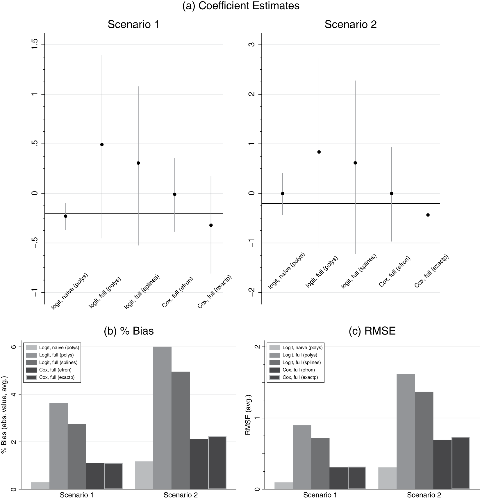
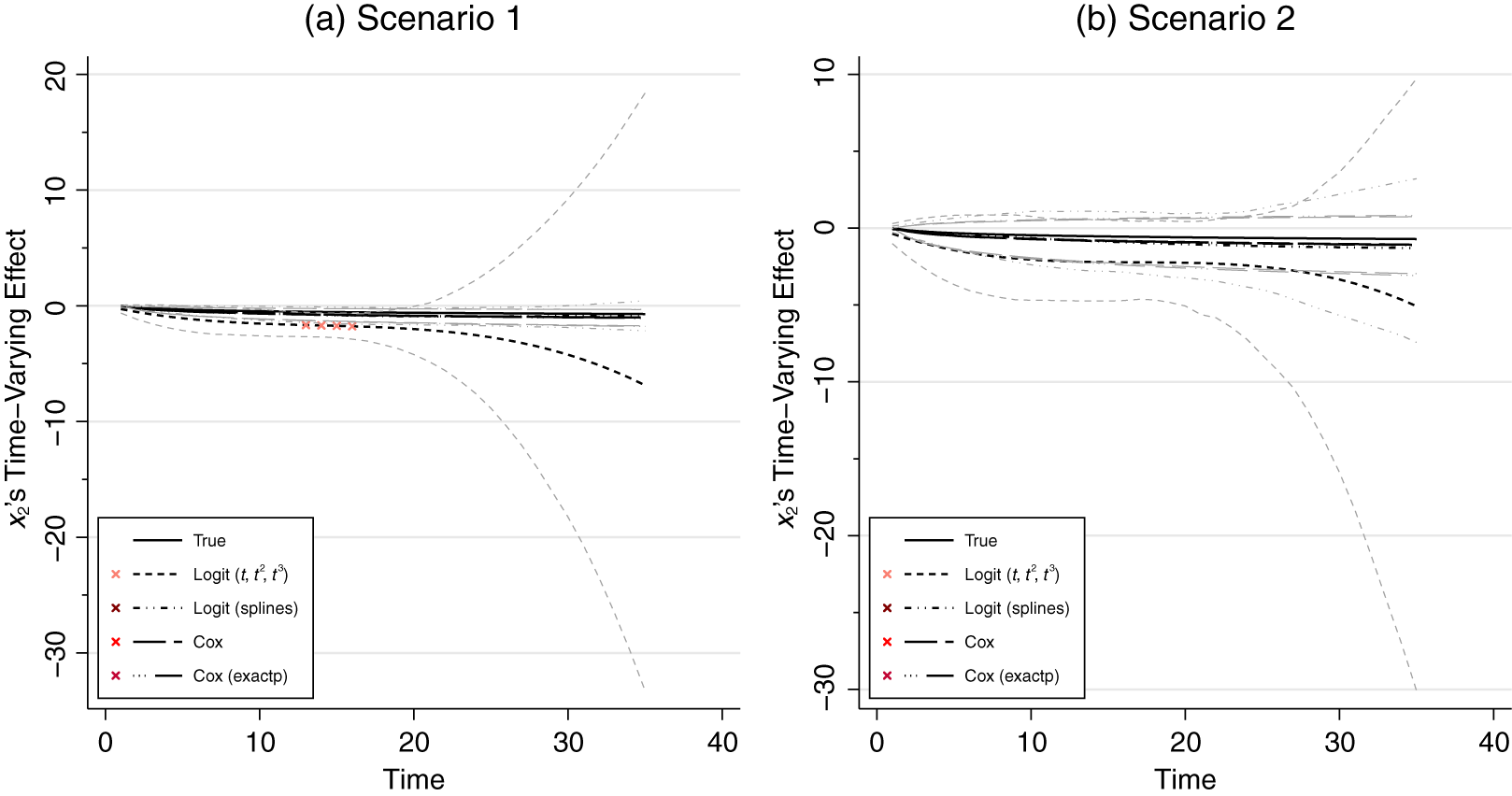
We discuss only broad trends here, but we provide our full set of complex process simulation results in our Supplemental Materials using a web-based viewing app.Footnote 20 Figure 2 (main coefficient effects) and Figure 3 (time-varying effects) show the results for Transition 2 from one of the 162 different parameter combinations we run, to serve as an illustrative example of the trends we note.
Complex simulation results—DGP = coerced start–stop, Transition 2 (main effect).

Complex simulation results—DGP = coerced start–stop, Transition 2 (TVEs).

4.2.2. Coefficient Estimates
We begin by examining the coefficient estimates themselves. In general, our complex simulation results largely mirror our conclusions from our simpler simulations. When we specify (1) a continuous-time DGP coerced into a start–stop format and (2) no PH violations are present, the Cox model with either tie correction consistently returns unbiased estimates of x’s main effect for both Transitions 1 and 2, as does the logit with either cubic polynomials or splines.
When we introduce PH violations for the coerced start–stop scenarios, we now must check the estimates of x’s main effect (Figure 2) and x’s time-varying effect (TVE; Figure 3). Regarding x’s main effect, our benchmark naïve logit model tends to return estimates farther from the parameter’s true value, unsurprisingly, to the point of being biased in some situations. By contrast, the properly specified logit and Cox specifications all return unbiased estimates of x’s main effect. The same is generally true for estimates of x’s TVE, although, on occasion, the logit with cubic polynomials returns some biased estimates for mid-sized t values (e.g., Figure 3a). The logit with polynomials is also the most prone to divergences from the truth for higher t values, although the true TVE value still falls within the estimates’ corresponding CIs (e.g., Figure 3, either panel).
Moving to percent bias and RMSE, the Cox model consistently outperforms both logits with TVEs on both criteria for coerced start–stop data with PH violations, consistent with our simple simulation results. The only scenarios in which the logit outperforms the Cox model in these metrics is when no PH violation exists. In these cases, a naïve logit model, which omits any TVEs, has lower percent bias and RMSE than the Cox or logit models with TVEs. In practice, these results still suggest that the Cox is preferable, as researchers who find no evidence of PH violations in their data typically omit these time-varying terms from their model. Their model specifications reduce to the simpler specifications covered by our earlier simulation results, with all the ensuing benefits. Switching our true DGP to discrete time yields similar results as coerced start–stop.
4.2.3. Predicted Quantities
We also consider these models’ predicted quantities when we introduce PH violations and causal complexity into the simulations. Space constraints prevent us from including illustrative figures in text, but all are available in our supplemental viewing app. Interestingly, we find that for discrete DGPs, the Cox and the logit consistently return unbiased transition probability estimates, regardless of the tie correction (Cox) or polynomials versus splines (logit).
For coerced start–stop, the Cox and the logit continue to perform similarly, but with a slight edge to the Cox. The Cox model returns consistently unbiased transition probability estimates. The logit models also typically return unbiased transition probability estimates. There are only a few exceptions for several scenarios involving a limited number of time points when Transition 1’s baseline hazard is monotonically increasing, but Transition 2’s baseline hazard is monotonically decreasing. Across all the scenarios, the Cox (efron)’s transition probabilities are closer to the true value than either logits’ transition probabilities—an important point, because it means the Cox typically does less poorly than logit, in line with our overarching claim.
On the whole, our complex simulations reinforce our conclusion from our simple simulations: the Cox model performs at least as well as both logit alternatives, and frequently better, when addressing more complex situations commonly present in BTSCS data. This is all the more true when considering our earlier point about logit’s estimating burden relative to the Cox in these contexts.
5. Application
We employ an application regarding MID onset to demonstrate the potential pitfalls of using L/P models for BTSCS data, and how Cox models provide an elegant alternative. Our data come from Oneal and Russett (Reference Oneal and Russett2005), covering 1885–2000 with a dyad-year unit of analysis. This dataset’s dependent variable is coded 1 for dyad-years in which the two states begin a new MID and 0 otherwise. We use the classic “liberal-realist” specification in our example, which are a set of control variables fairly standard across studies of MID onset. While the original analysis focuses exclusively on MID onset, we expand this focus to show how considering the event’s duration can offer novel insights. We also use the application to demonstrate the importance of testing the PH assumption for both the event’s onset and its duration, as different covariates can violate the assumption for each outcome.
5.1. Model Estimates and PH Testing
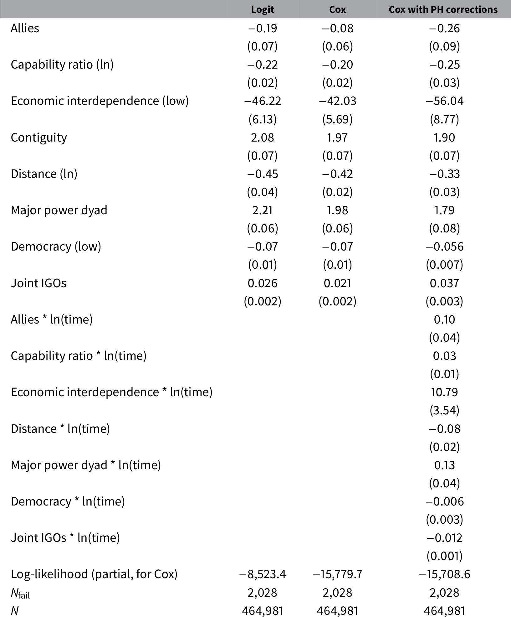
Table 2’s first two columns compare the logit and Cox model estimates for Oneal and Russett’s original dependent variable of MID onset. To ensure these models yield equivalent conclusions, we include a cubic polynomial for the number of years since the last MID onset in the logit model. The two models’ results are largely similar, and support most of the established conclusions regarding MID onset. For instance, both models indicate higher levels of economic interdependence reduce the risk of dyadic MID onset, as do greater distances between the two states and larger disparities in the two states’ relative capabilities.
MID onset—comparing logit and Cox estimates.

Notes: Two-tailed p-values used for discussions of significance. Standard errors reported in parenthesis. Cox model estimated with Efron tie correction. Logit model also includes peace year cubic polynomials.
Abbreviations: IGO, intergovernmental organization; MID, militarized interstate dispute; PH, proportional hazard.
While the two models’ estimates are similar, the Cox specification presents a central advantage over the logit model: it allows us to test for PH violations more easily, and correcting for PH violations also consumes fewer degrees of freedom. We find a number of violations when we test for PH violations in both the Cox and the logit.Footnote 21 When we correct for them (Table 2, third column), the model results change from the naïve estimates presented in the previous two columns. Economic interdependence’s estimate is negative, large, and significant at the 0.05 level, indicating that higher levels of economic interdependence greatly reduce the risk of MID onset. However, economic interdependence’s time interaction is positively signed and significant at the 0.05 level. The constituent and interaction terms together indicate that immediately following a MID (t = 0), higher levels of economic interdependence greatly reduce the risk of another MID onset. As time passes, although, this pacifying effect grows smaller and smaller.Footnote 22 This is an important scope condition on a core finding in the study of MID onset: greater levels of economic interdependence do reduce the risk of MID onset, but this effect is strongest in the immediate aftermath of a MID and tends to decline over time.Footnote 23
5.2. Causal Complexity
An additional advantage of Cox models compared to L/P models is their flexibility in modeling political processes characterized by causal complexity (Metzger and Jones Reference Metzger and Jones2016) while avoiding the pitfalls described by McGrath (Reference McGrath2015). For MIDs, we divide the process into two stages: peace and an ongoing MID. Our new dependent variable is coded 1 if a transition occurs between the stages in that year, amounting to whether a MID onset or termination occurred. We account for causal complexity by using transition-specific covariates. Importantly, if the same variable of interest exerts one effect on MID onset but another, different effect on MID termination, our modeling strategy will detect and model the difference.Footnote 24
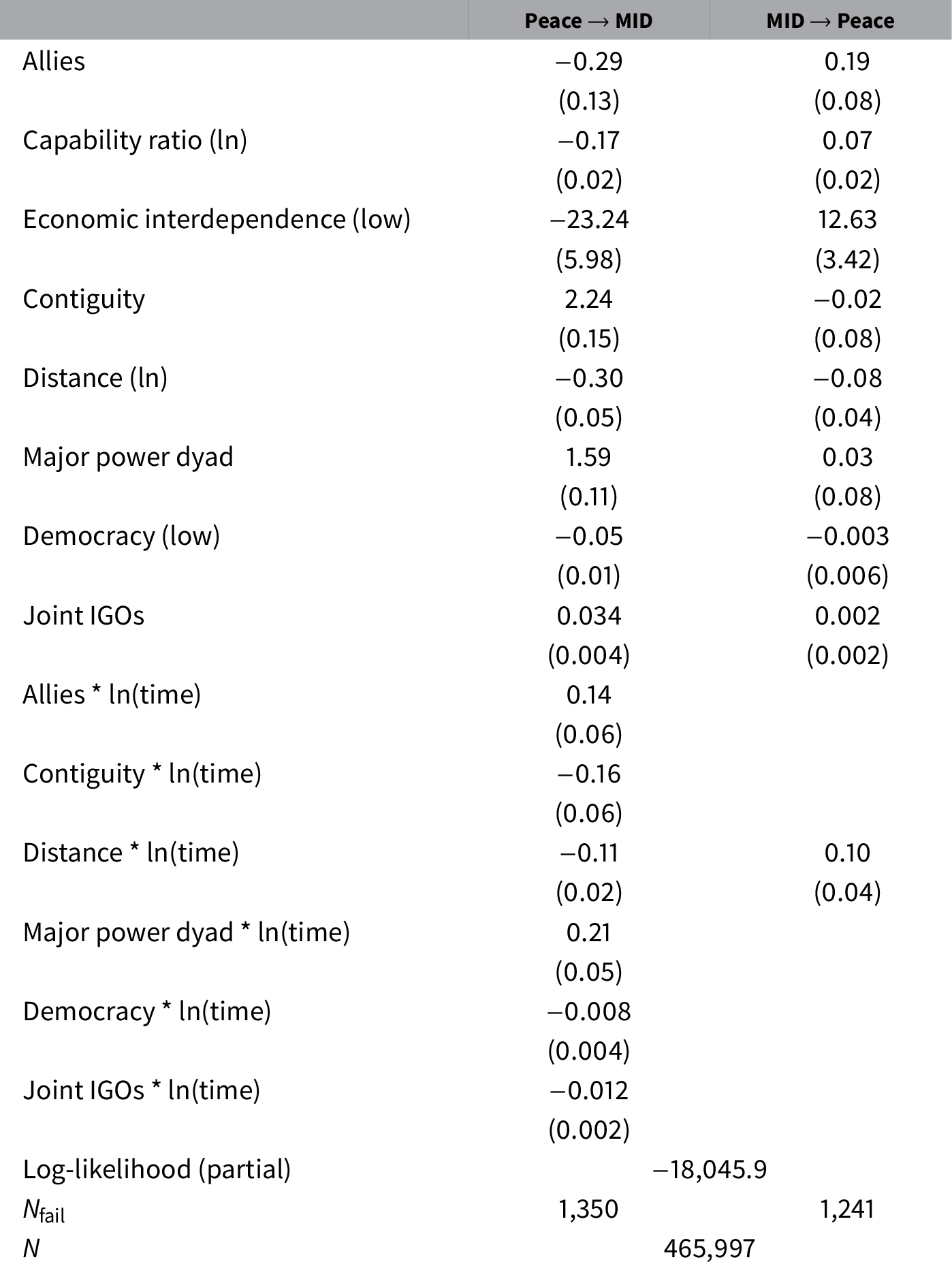
Table 3 presents our multistate Cox model results. The first column contains the estimates for each covariate’s effect on MID onset, and the second column contains the estimates for MID termination, equivalent to a transition from an ongoing MID to peace. We tested for PH violations for both transitions and implemented corrections accordingly.Footnote 25 These results demonstrate the importance of accounting for causal complexity. Consider regime type’s effect when operationalized as the least democratic country within the dyad; both the constituent and interaction terms are significant at the 0.05 level. As this country becomes more democratic, the risk of MID onset declines (Peace → MID). With the time interaction, this effect grows increasingly negative, meaning that democracy plays an even greater role in reducing the risk of MID onset as peace endures. However, regime type has no significant effect on MID duration (MID → Peace). Both results together indicate democracy may be helpful in avoiding MIDs in the first place, but if a MID does start, democracy plays little role in reducing the MID’s duration. Without differentiating between these two distinct transitions, regime type’s different effects might be overlooked, which Cox models allow us to do more easily than L/P.Footnote 26
MID onset and termination—multistate model.

Notes: Two-tailed p-values used for discussions of significance. Standard errors reported in parenthesis. Model estimated using Efron tie correction.
Abbreviations: IGO, intergovernmental organization; MID, militarized interstate dispute.
6. Conclusion
When confronted with BTSCS data, how can researchers most readily account for duration dependence, and then make unbiased substantive inferences? We contend researchers should consider using Cox models when confronted with BTSCS data, rather than L/P models. Cox models are better able to accommodate additional features implied by duration dependence than L/P, because while both models have the technical capacity to address these additional features, Cox models use fewer degrees of freedom to do so, allowing them to produce accurate estimates under a far wider range of conditions than L/P.
In our initial simulations, we verified that the logit and the Cox produce comparable, correct estimates of simple duration processes. Notably, though, while both the Cox and the logit returned unbiased coefficient estimates in general, the Cox’s estimates were closer to the truth across all our scenarios. This theme carried through to our main, more complex simulations: the Cox performs at least as well as the logit. However, the Cox often performs quite better in scenarios frequently encountered by political scientists. We highlighted the Cox model’s ability to readily address three issues more easily than L/P: easily testing and correcting for PH violations, easily modeling causally complex processes, and removing concerns about baseline hazard misspecification. Moreover, our simulations demonstrated that while both the Cox and the logit typically return unbiased coefficient estimates for both the main effect and the time-varying effect, the Cox is much more efficient, consistently returning lower RMSEs.
Our MID application demonstrates the potential limitations of L/P in the context of BTSCS data, and the flexibility and intuitive appeal of Cox models as an alternative. Here, too, we highlighted three things. First, the application showcased the ramifications of violating the PH assumption in L/P. Second, this application highlighted the flexibility of Cox models by readily accounting for causal complexity in several forms. Finally, transition probabilities provide a straightforward way to substantively interpret Cox model results, even from models that involve multiple PH corrections and causally complex processes. We discuss this more fully in online Appendix B, as well as in other work (Jones and Metzger Reference Jones and Metzger2019).
The ubiquity of BTSCS data in political science makes identifying appropriate methods of analysis paramount. Regardless of whether researchers’ hypotheses involve duration dependence, we must account for it, because failing to do so amounts to misspecification bias, affecting our inferences’ validity. Yet in many ways, the standard practice in political science to use L/P with time counters to model duration dependence has an easier alternative. Our suggestion—to use Cox models—gives researchers leverage to more readily address and model the complications arising from BTSCS data.
Acknowledgments
This paper was presented as part of the 2016–2017 International Methods Colloquium series, and was also presented at the 2017 annual APSA meeting, the University of Minnesota’s Political Methodology Colloquium, The Ohio State University’s PRISM workshop, and the University of Virginia’s Quantitative Collaborative. We thank Susan Hannah Allen, Neal Beck, Jeff Carter, Matt DiGiuseppe, Shuai Jin, and Jane Lawrence Sumner for feedback on earlier drafts. We used William & Mary’s high-performance computing cluster to run some of our simulations and thank the staff for their support. We bear sole responsibility for any remaining errors and shortcomings.
Data Availability Statement
All analyses are performed using Stata 15.1. Replication code for this article has been published through Code Ocean and can be viewed interactively at https://doi.org/10.24433/CO.7111207.v2 (Metzger and Jones Reference Metzger and Jones2021a). A preservation copy of the same code and data can also be accessed via Dataverse at https://doi.org/10.7910/DVN/FEW2JP (Metzger and Jones Reference Metzger and Jones2021b).
Supplementary Material
To view supplementary material for this article, please visit https://doi.org/10.1017/pan.2021.14.