



1. Introduction
Thermally driven convection is ubiquitous, occurring in natural systems such as atmospheric circulation (Hartmann et al. Reference Hartmann, Moy and Fu2001), oceanic thermohaline circulation (Marshall & Schott Reference Marshall and Schott1999) and mantle convection (Schubert et al. Reference Schubert, Turcotte and Olson2001), as well as in industrial applications, such as heat exchangers, chemical reactors and crystal growth (Brown Reference Brown1988; Poitevin et al. Reference Poitevin, Boccaccini, Dell’Orco, Diegele, Lässer, Salavy, Sundström and Zmitko2007; Lohse & Shishkina Reference Lohse and Shishkina2023). A classic paradigm for studying thermally driven flows is Rayleigh–Bénard convection (RBC) (for reviews, see for example, Ahlers et al. Reference Ahlers, Grossmann and Lohse2009; Lohse & Xia Reference Lohse and Xia2010; Xia Reference Xia2013; Xia et al. Reference Xia, Huang, Xie and Zhang2023), while vertical convection (VC), in which a fluid layer is confined between two isothermal vertical walls held at different temperatures, represents a distinct and equally fundamental class of convection (Shishkina Reference Shishkina2016; Wang et al. Reference Wang, Liu, Verzicco, Shishkina and Lohse2021). Vertical convection is directly relevant to many engineering systems, including double-glazed curtain walls, heat sink fins for electronic equipment and nuclear reactor cooling, where the alignment of the buoyancy force with the boundary layer plays a crucial role (Batchelor Reference Batchelor1954; Ng et al. Reference Ng, Ooi, Lohse and Chung2015).
Although both RBC and VC are governed by the same dimensionless control parameters, namely the Rayleigh number
 $\textit{Ra}$
, the Prandtl number
 $\textit{Pr}$
and the aspect ratio
 $A$
, their physical mechanisms differ significantly. Here,
 $\textit{Ra}$
characterises the strength of buoyancy forcing,
 $\textit{Pr}$
measures the ratio of momentum diffusivity to thermal diffusivity and
 $A$
quantifies the geometric confinement of the domain; see equation (2.4) for their definitions. In turbulent RBC, heat transport is primarily driven by unstable thermal stratification and the continuous emission of thermal plumes from the horizontal top and bottom boundaries (Ahlers et al. Reference Ahlers, Grossmann and Lohse2009). By contrast, VC is distinguished by the coexistence of wall-bounded shear layers near the vertical walls, where buoyancy forcing acts parallel to the vertical walls, and a stably stratified bulk region (Shishkina Reference Shishkina2016; Zhu et al. Reference Zhu, Chen, Qin and Ni2025). This distinctive coupling among wall shear, stable stratification and recirculating flow structures gives rise to transport mechanisms that are qualitatively different from those in turbulent RBC.
Despite its distinct physical characteristics and broad engineering relevance, VC has historically received considerably less attention than RBC. Consequently, several fundamental issues in VC, including flow state transitions, bulk stratification and transport scaling, remain incompletely understood. In the following, we review previous studies on these topics and thereby motivate the present investigation of aspect-ratio effects on flow state evolution, bulk stratification and transport scaling in VC.
1.1. Flow state evolution
One of the central questions in VC concerns the evolution of flow states as the thermal driving strength increases. Unlike the convective instability in RBC (Rayleigh Reference Rayleigh1916; Chandrasekhar Reference Chandrasekhar1961), convective motion in VC can be induced by any non-zero temperature difference between the vertical walls (Batchelor Reference Batchelor1954; Le Quéré & Behnia Reference Le Quéré and Behnia1998). At sufficiently low
 $\textit{Ra}$
, the system exhibits a weak, steady circulation where heat is mainly transported by conduction. As
 $\textit{Ra}$
increases, the core of the domain develops a stably stratified bulk region, and the flow becomes confined to the narrow boundary layers near the isothermal walls (Oshima Reference Oshima1971; Jaluria & Gebhart Reference Jaluria and Gebhart1974). With further increases in
 $\textit{Ra}$
, the flow destabilises and exhibits periodic, quasi-periodic or chaotic dynamics (Paolucci & Chenoweth Reference Paolucci and Chenoweth1989), eventually transitioning to fully developed turbulence at sufficiently high
 $\textit{Ra}$
(Chenoweth & Paolucci Reference Chenoweth and Paolucci1986).
Subsequent studies have revealed that the instability scenario in VC depends sensitively on both
 $\textit{Pr}$
and
 $A$
, as these parameters control the relative importance of shear in the boundary layers near the wall, corner turning regions and buoyancy-driven internal-wave activity in the stratified bulk. For a square cavity with
 $A=1$
, systematic variation of
 $\textit{Pr}$
showed that the transition pathway changes qualitatively with fluid properties (Janssen & Henkes Reference Janssen and Henkes1995). At moderate
 $\textit{Pr}$
(
 $0.25 \le \textit{Pr} \le 2$
), the flow follows a transition sequence from steady to periodic and then quasi-periodic dynamics, driven by two distinct shear-related bifurcations: one originating in the corner turning layer, where the vertical wall jet bends horizontally and excites internal gravity waves, and the other arising directly within the vertical wall boundary layer. At higher
 $\textit{Pr}$
(
 $2.5 \le \textit{Pr} \le 7$
), the transition becomes more abrupt, with the flow jumping directly from steady to chaotic dynamics, accompanied by a marked increase in the critical Rayleigh number for the onset of oscillations.
The influence of aspect ratio
 $A$
on flow evolution has been examined in several studies, collectively indicating that
 $A$
governs not only the critical conditions for instability but also the dominant destabilisation mechanisms. In air-like conditions with
 $\textit{Pr}=0.71$
, increasing
 $A$
from 1 to
 $100$
leads to progressively stronger boundary-layer interaction and enhanced unsteadiness (Chenoweth & Paolucci Reference Chenoweth and Paolucci1986). For aspect ratios near unity, the dominant instability mechanism shifts with
 $A$
: internal-wave-type instabilities prevail in the stratified interior at smaller
 $A$
, whereas shear instabilities of the wall boundary layers become more prominent at larger
 $A$
(Paolucci & Chenoweth Reference Paolucci and Chenoweth1989). More recent studies have further highlighted the role of geometric confinement in shaping flow organisation and transport. In liquid-metal VC with
 $\textit{Pr} \ll 1$
, increasing
 $A$
from
 $1$
to
 $5$
concentrates heat transport near the top and bottom regions while diminishing the bulk contribution (Zwirner et al. Reference Zwirner, Emran, Schindler, Singh, Eckert, Vogt and Shishkina2022). Meanwhile, combined numerical simulations and linear stability analyses have shown that both
 $\textit{Pr}$
and
 $A$
strongly modulate the emerging flow patterns: low-
 $\textit{Pr}$
flows are dominated by large-scale convective cells, whereas higher
 $\textit{Pr}$
promotes smaller, more localised circulations; for
 $A\lt 1$
, dynamics remain confined to near-wall regions with limited internal-wave activity, while increasing
 $A$
fosters a more stratified organisation where internal waves become increasingly prominent (Khoubani et al. Reference Khoubani, Mohanan, Augier and Flór2024).
Despite these important insights, the available evidence is still largely confined to a limited set of aspect ratios. As summarised in table 1, systematic investigations that map the evolution of flow states across a broad range of
 $A$
, especially extending to the low-aspect-ratio confined regime, remain absent.
Summary of parameter range of VC from previous studies and the present work. Here
 $\textit{Ra}$
and
 $\textit{Pr}$
are the Rayleigh and Prandtl numbers, respectively;
 $A$
is the aspect ratio. For rectangular cells with plate height
 $L$
and plate spacing
 $H$
,
 $A = L/H$
. For cylindrical cells,
 $A= D/H$
, with
 $D$
being the diameter of the cell and
 $H$
being the plate spacing. The references are grouped into 3-D studies (including experiments and 3-D DNS), 2-D DNS and the present work, to facilitate a direct comparison across different dimensionalities. The scaling exponents
 $\beta$
and
 $\gamma$
correspond to
 $\textit{Nu}\sim Ra^\beta$
and
 $\textit{Re}\sim Ra^\gamma$
, respectively, based on the original definitions in each reference. The references are (
 $a$
) Oshima (Reference Oshima1971); (
 $b$
) Ng et al. (Reference Ng, Ooi, Lohse and Chung2015); (
 $c$
) Shishkina (Reference Shishkina2016); (
 $d$
) Howland et al. (Reference Howland, Ng, Verzicco and Lohse2022); (
 $e$
) Zwirner et al. (Reference Zwirner, Emran, Schindler, Singh, Eckert, Vogt and Shishkina2022); (
 $f$
) Trias et al. (Reference Trias, Soria, Oliva and Pérez-Segarra2007, Reference Trias, Gorobets, Soria and Oliva2010); (
 $g$
) De Vahl Davis (Reference De Vahl Davis1983); (
 $h$
) Chenoweth & Paolucci (Reference Chenoweth and Paolucci1986); (
 $i$
) Paolucci & Chenoweth (Reference Paolucci and Chenoweth1989); (
 $j$
) Janssen & Henkes (Reference Janssen and Henkes1995); (
 $k$
) Xin & Le Quéré (Reference Xin and Le Quéré1995); (
 $l$
) Le Quéré & Behnia (Reference Le Quéré and Behnia1998); (
 $m$
) Wang et al. (Reference Wang, Liu, Verzicco, Shishkina and Lohse2021); (
 $n$
) Khoubani et al. (Reference Khoubani, Mohanan, Augier and Flór2024); (
 $o$
) present work. The studies of (
 $b$
) Ng et al. (Reference Ng, Ooi, Lohse and Chung2015) and (
 $d$
) Howland et al. (Reference Howland, Ng, Verzicco and Lohse2022) employ periodic boundary conditions in the vertical direction, corresponding to the
 $A\to \infty$
limit of unbounded VC.

Table 1. Long description
A table comparing parameter ranges from different studies on VC. The table has 15 rows and 8 columns. The columns are labeled Ref., Method, Ra range, Pr range, A range, Geom., β and γ. The rows are labeled with references and corresponding values for each parameter range. Each row provides specific values for the Rayleigh number (Ra), Prandtl number (Pr), aspect ratio (A), geometry (Geom.), and scaling exponents (β and γ). The references are grouped into 3-D studies, 2-D DNS, and the present work. The table includes a variety of methods such as EXP, 3-D DNS, and 2-D DNS. The values for Ra range from 10^2 to 10^14, Pr ranges from approximately 10^-2 to 10^2, and A ranges from 0.5 to infinity. The geometries include rectangular and cylindrical cells. The scaling exponents β and γ vary across the studies.
1.2. Bulk stratification
A defining characteristic of VC is the spontaneous formation of a stably stratified bulk region (Oshima Reference Oshima1971; Ravi et al. Reference Ravi, Henkes and Hoogendoorn1994; Trias et al. Reference Trias, Soria, Oliva and Pérez-Segarra2007; Sebilleau et al. Reference Sebilleau, Issa, Lardeau and Walker2018; Chong et al. Reference Chong, Yang, Wang, Verzicco and Lohse2020). This feature bears strong similarity to stably stratified flows in geophysical and astrophysical systems, such as atmospheric inversions, oceanic pycnoclines and stellar radiative zones, making VC an idealised model for studying stratification-controlled transport.
The stratification strength
 $S$
, defined as the dimensionless vertical temperature gradient at the domain centre, is a critical measure of the system’s dynamical state, i.e.
 \begin{equation} S\equiv \langle (\partial T/\partial z )_c /( \Delta T/H ) \rangle _t, \end{equation}
where the subscript ‘
 $c$
’ denotes the domain centre and
 $\left \langle \boldsymbol{\cdot }\right \rangle _t$
means time averaging. The current understanding of bulk stratification in VC remains incomplete and strongly depends on
 $\textit{Pr}$
. In the high-
 $\textit{Pr}$
limit the classical asymptotic theory derived by Gill (Reference Gill1966) predicts a stratification strength of
 $S=0.42$
in the asymptotic limit
 $\textit{Ra}\to \infty$
. This theoretical framework was subsequently refined by Blythe et al. (Reference Blythe, Daniels, Simpkins and Stewartson1997), who obtained an updated prediction of
 $S=0.52$
. These asymptotic predictions have been supported by numerical studies in high-
 $\textit{Pr}$
fluids. For example, Ravi et al. (Reference Ravi, Henkes and Hoogendoorn1994) reported stratification strengths at
 $\textit{Pr}=70$
that are in close agreement with the refined theoretical prediction, yielding
 $S=0.52$
. Such an agreement suggests that the asymptotic framework provides a reliable description of bulk stratification in the high-
 $\textit{Pr}$
regime.
By contrast, the situation is much less clear for moderate- and low-
 $\textit{Pr}$
fluids. In these regimes, the bulk stratification deviates substantially from the high-
 $\textit{Pr}$
asymptotic theory, and no complete theoretical description is available. Although Graebel (Reference Graebel1981) proposed an approximate solution for finite
 $\textit{Pr}$
, the derivation involved neglecting several terms in the governing equations, which led to noticeable quantitative discrepancies when compared with direct numerical simulation (DNS). For example, at
 $\textit{Pr}=0.71$
, the predicted value
 $S=0.49$
is significantly smaller than DNS results, which typically yield
 $S=O(1)$
under comparable conditions (Ravi et al. Reference Ravi, Henkes and Hoogendoorn1994; Trias et al. Reference Trias, Soria, Oliva and Pérez-Segarra2007).
In addition, the dependence of
 $S$
on
 $\textit{Ra}$
reveals complex behaviours. Earlier DNS studies suggested that, for moderate thermal driving (
 $\textit{Ra}\le 10^{10}$
), the bulk stratification exhibits only weak sensitivity to
 $\textit{Ra}$
(Paolucci Reference Paolucci1990). However, extensive DNS over a very wide range of
 $\textit{Ra}$
by Wang et al. (Reference Wang, Liu, Verzicco, Shishkina and Lohse2021) revealed a complex multi-regime behaviour. Specifically, for
 $\textit{Pr}=10$
and
 $A=1$
, they identified three distinct regimes: regime I (
 $\textit{Ra} \lesssim 5 \times 10^{10}$
), in which the centre temperature gradient
 $S$
is approximately constant; regime II (
 $5 \times 10^{10} \lesssim Ra \lesssim 10^{13}$
), in which
 $S$
displays a non-monotonic dependence on
 $\textit{Ra}$
, first increasing and then decreasing; and regime III (
 $\textit{Ra} \gtrsim 10^{13}$
), a second plateau regime in which
 $S$
becomes weakly dependent on
 $\textit{Ra}$
again but with a smaller value than in regime I. These transitions were attributed to changes in the boundary-layer structure and the onset of bulk turbulence, respectively.
Despite these advances, existing studies have focused almost exclusively on fixed geometries, most commonly the square cavity with
 $A=1$
(De Vahl Davis Reference De Vahl Davis1983; De Vahl Davis & Jones Reference De Vahl Davis and Jones1983; Ravi et al. Reference Ravi, Henkes and Hoogendoorn1994). The influence of aspect ratio on bulk stratification remains largely unexplored, which serves as one of the motivations of the present study.
1.3. Transport scaling
A central issue in VC is the scaling behaviour of global heat and momentum-transport efficiency, commonly expressed as
 $\textit{Nu} \sim Ra^{\beta }$
and
 $\textit{Re} \sim Ra^{\gamma }$
(Shishkina Reference Shishkina2016). Here
 $\textit{Nu}$
is the Nusselt number and Re is the Reynolds number. Unlike the well-established scaling frameworks in RBC (Grossmann & Lohse Reference Grossmann and Lohse2000, Reference Grossmann and Lohse2001, Reference Grossmann and Lohse2002; Lohse Reference Lohse2004; Stevens et al. Reference Stevens, van der Poel, Grossmann and Lohse2013), the corresponding scaling laws in VC remain to be settled.
From a theoretical perspective, Shishkina (Reference Shishkina2016) derived scaling relations for laminar VC and validated them by DNS, obtaining
 $\textit{Nu} \sim \textit{Pr}^{1/4} \textit{Ra}^{1/4}$
,
 $\textit{Re} \sim \textit{Pr}^{-1/2}Ra^{1/2}$
for
 $\textit{Pr} \ll 1$
and
 $\textit{Nu} \sim \textit{Pr}^{0}Ra^{1/4}$
,
 $\textit{Re} \sim \textit{Pr}^{-1}Ra^{1/2}$
for
 $\textit{Pr} \gg 1$
. For turbulent VC in the high-
 $\textit{Ra}$
limit with a large aspect ratio, Ching (Reference Ching2023) showed that the Nusselt number and the friction Reynolds number scale as
 $\textit{Nu} \sim Ra^{1/3}$
and
 $\textit{Re}_{\tau } \sim Ra^{1/3}$
, respectively. Building on this framework, Ng & Ching (Reference Ng and Ching2026) proposed an eddy thermal diffusivity model that yields universal scaling functions for the mean temperature profiles in the near-wall and outer regions. More generally, Ng et al. (Reference Ng, Ooi, Lohse and Chung2015) extended the Grossmann–Lohse framework to VC and argued that the effective scaling behaviour depends on the relative contributions of boundary layer and bulk dissipation. The above studies imply that a single power-law relation may not hold across the entire
 $\textit{Ra}-\textit{Pr}-A$
parameter space.
Consistent with this view, previous numerical studies have reported noticeably different effective exponents depending on the parameter range and geometry of the domain. In two-dimensional (2-D) square cavities (
 $A=1$
) at
 $\textit{Pr}=0.71$
, Le Quéré & Behnia (Reference Le Quéré and Behnia1998) found
 $\beta = 1/4$
up to
 $\textit{Ra}=10^{10}$
, while Wang et al. (Reference Wang, Xia, Yan, Sun and Wan2019) obtained
 $\beta \approx 0.27$
and
 $\gamma \approx 0.50$
over
 $10^5 \leq Ra \leq 10^9$
. In vertically elongated cavities with
 $A=4$
, high-
 $\textit{Ra}$
DNS often reported heat-transport exponents close to the laminar prediction
 $\beta = 1/4$
, even in the turbulent regimes (Xin & Le Quéré Reference Xin and Le Quéré1995; Trias et al. Reference Trias, Soria, Oliva and Pérez-Segarra2007, Reference Trias, Gorobets, Soria and Oliva2010). For three-dimensional (3-D) simulations with periodic boundary conditions in the streamwise and spanwise directions, Ng et al. (Reference Ng, Ooi, Lohse and Chung2015) reported an effective exponent
 $\beta = 0.31$
at
 $\textit{Pr}=0.709$
over
 $10^5 \leq Ra \leq 10^9$
, while Ng et al. (Reference Ng, Spandan, Verzicco and Lohse2020) confirmed
 $\beta = 1/4$
and
 $\gamma = 1/2$
for
 $10^8 \leq Ra \leq 1.3 \times 10^9$
.
Extending the study of VC to much higher thermal driving, Wang et al. (Reference Wang, Liu, Verzicco, Shishkina and Lohse2021) performed 2-D DNS for
 $\textit{Pr}=10$
over a broad range
 $10^7 \leq Ra \leq 10^{14}$
in an
 $A=1$
domain. They identified three distinct flow regimes based on the behaviour of the centre vertical temperature gradient
 $S$
. In regime I (
 $\textit{Ra} \lesssim 5 \times 10^{10}$
), the flow remains steady and the scaling exponents
 $\beta \approx 0.26$
and
 $\gamma \approx 0.51$
agree well with the laminar predictions of Shishkina (Reference Shishkina2016). In regime II (
 $5 \times 10^{10} \lesssim Ra \lesssim 10^{13}$
), the onset of unsteadiness and plume ejection leads to a non-monotonic variation of
 $S$
, with
 $\beta$
increasing to approximately
 $1/3$
and
 $\gamma$
decreasing to approximately
 $4/9$
. In regime III (
 $\textit{Ra} \gtrsim 10^{13}$
), efficient mixing in the bulk produces a well-mixed interior and layered structures near the horizontal walls, while the scaling exponents remain close to those of regime II. These results demonstrate that the transport scaling in VC undergoes a sharp transition from
 $\beta = 1/4$
to
 $\beta \approx 1/3$
at high
 $\textit{Ra}$
, rather than a smooth crossover as observed in RBC.
To provide an overview of the existing parameter space and to highlight the methodological distinctions among previous studies, we have summarised the key parameters and reported transport scaling exponents in table 1. Notably, by grouping the available data into 2-D and 3-D set-ups, the table shows that while the momentum-transport exponent
 $\gamma$
remains consistently close to 0.5 across both 2-D and 3-D domains, the heat-transport exponent
 $\beta$
exhibits considerable scatter ranging from 0.25 to 1/3 that cannot be attributed solely to the distinction between 2-D and 3-D set-ups, but rather reflects the combined dependence on
 $\textit{Ra}, \textit{Pr}, A$
, and the specific geometry of the individual study. Despite these quantitative differences, most existing scaling studies are confined to discrete geometries – predominantly square cavities or specific elongated cases, a systematic investigation of the geometric confinement effects over a wide range of aspect ratios, especially in the low-aspect-ratio regime, remains absent in both 2-D and 3-D studies. The influence of aspect ratio on transport scaling laws has not been systematically examined. Thus, understanding how
 $A$
affects these transport relationships remains essential for both theoretical insights and practical applications involving VC, which serves as another motivation for the present study.
In this paper we employ 2-D DNS to systematically investigate the effects of aspect ratio on the flow state evolution, bulk stratification and transport efficiency in VC over a broad parameter space. The paper is organised as follows. Section 2 describes the governing equations and the numerical method employed. Section 3 presents the main findings, focusing on how geometric confinement shapes the flow organisation and heat transport. In § 3.1 we construct a phase diagram in the
 $\textit{Ra}-A$
space to map the flow state evolution under geometric confinement. The variation of bulk stratification strength with
 $A$
and its underlying physical mechanisms are analysed in § 3.2. Furthermore, in § 3.3 we quantify the impact of
 $A$
on global heat and momentum transport, identifying an optimal aspect ratio that maximises heat-transport efficiency. In § 3.4 we compare
 $H$
- and
 $L$
-based non-dimensionalisations to determine the most appropriate length scale for VC. Finally, we summarise the key findings and outline future work in § 4.
(
 $a$
) Schematic of the 2-D VC system considered in the present study with an aspect ratio of
 $A=2$
. (b) The
 $\textit{Ra}_H-A$
parameter space covered in this study.

2. The numerical set-up and verification
We consider a 2-D VC system in a rectangular domain with aspect ratio
 $A=L/H$
, where
 $L$
is the plate height and
 $H$
is the plate spacing. A schematic of the system for a representative case with
 $A = 2$
is shown in figure 1(a). For the velocity boundary conditions, no-slip and impermeable conditions are imposed on all solid boundaries. For the temperature boundary conditions, the left vertical wall is held at a constant cold temperature
 $T_c = -0.5$
, while the right vertical wall is maintained at a constant hot temperature
 $T_h = 0.5$
. The top and bottom horizontal walls are adiabatic, satisfying
 $\partial T/\partial z = 0$
. This configuration establishes a sustained horizontal temperature gradient that drives the convective flow.
The flow is simulated under the Oberbeck–Boussinesq approximation (Oberbeck Reference Oberbeck1879; Boussinesq Reference Boussinesq1903), in which the fluid density
 $\rho$
is assumed to vary linearly with temperature
 $T$
according to
 $\rho = \rho _0[1 - \alpha (T - T_0)]$
. Here,
 $\rho _0$
and
 $T_0$
are the reference density and temperature, respectively, with
 $T_0$
taken as the mean temperature of the two vertical walls, i.e.
 $(T_h+T_c)/2$
, and
 $\alpha$
is the thermal expansion coefficient. Under this approximation, density variations are neglected everywhere except in the buoyancy term of the momentum equation. The resulting dimensionless governing equations are
 \begin{equation} \boldsymbol{\nabla }\boldsymbol{\cdot }\boldsymbol{u} = 0 , \end{equation}
 \begin{equation} \frac {\partial \boldsymbol{u}}{\partial t} + (\boldsymbol{u}\boldsymbol{\cdot }\boldsymbol{\nabla })\boldsymbol{u} = -\boldsymbol{\nabla }\!p + \sqrt {\frac {\textit{Pr}}{\textit{Ra}}}{\nabla} ^2\boldsymbol{u} + \theta \hat {\boldsymbol{e}}_{z} , \end{equation}
 \begin{equation} \frac {\partial \theta }{\partial t} + (\boldsymbol{u}\boldsymbol{\cdot }\boldsymbol{\nabla })\theta = \frac {1}{\sqrt {\textit{RaPr}}}{\nabla} ^2\theta . \end{equation}
Here,
 $\boldsymbol{u}=(u,w)$
,
 $p$
and
 $\theta$
denote the velocity field, generalised pressure and temperature field, respectively. The unit vector in the vertical direction is denoted by
 $\hat {\boldsymbol{e}}_{z}$
. Equations (2.1)–(2.3) have been non-dimensionalised using the distance between the left cold and right hot plates
 $H$
, the imposed temperature difference
 $\Delta T$
between the two plates, the free-fall velocity
 $U_{ff} = \sqrt {\alpha g \Delta \textit{TH}}$
and the free-fall time
 $\tau _{ff} = H / U_{ff}$
. From these equations, the key dimensionless parameters governing the VC system are obtained as
 \begin{equation} \textit{Ra}_H = \frac {g \alpha \Delta \textit{TH}^3}{\nu \kappa }, \quad \textit{Pr} = \frac {\nu }{\kappa }, \qquad A = \frac {L}{H}, \end{equation}
which denote the Rayleigh number, the Prandtl number and the aspect ratio, respectively. Here,
 $\nu$
is the kinematic viscosity,
 $\kappa$
is the thermal diffusivity and
 $g$
is the gravitational acceleration constant. The subscript ‘
 $H$
’ indicates
 $H$
is used as the characteristic length scale. In § 3.4 the plate height
 $L$
will also be adopted as a characteristic length scale, and the corresponding quantities are denoted with the subscript ‘
 $L$
’. Similar definitions apply to other quantities with subscripts.
The response of the system is quantified by two dimensionless parameters, namely, the Nusselt number
 $\textit{Nu}_H$
, which measures the global heat-transport efficiency relative to the conductive heat flux, and the Reynolds number
 $\textit{Re}_H$
, which characterises the flow intensity. They are defined as
 \begin{equation} \textit{Nu}_H = \frac {Q}{\lambda \Delta T / H}, \quad \textit{Re}_H = \frac {U H}{\nu }, \end{equation}
where
 $Q$
is the total heat flux through the system,
 $\lambda$
is the thermal conductivity and
 $U$
is the characteristic velocity of the flow.
We solve the dimensionless governing equations (2.1)–(2.3) using the CUPS code, which is a finite-volume solver specifically developed for turbulent thermal convection. For details on the CUPS code and its verification, we refer the reader to Kaczorowski & Xia (Reference Kaczorowski and Xia2013), Kaczorowski et al. (Reference Kaczorowski, Chong and Xia2014) and Chong et al. (Reference Chong, Ding and Xia2018). Spatial discretisation is performed on a non-uniform Cartesian grid with
 $N_x \times N_z$
points in the
 $x$
and
 $z$
directions, respectively. Time integration follows an Euler–Leapfrog approach: the convection term is discretised with the leapfrog scheme and the diffusion term is discretised with the forward Euler method.
The parameter space explored in this study is shown in figure 1(b). We simulated 98 cases with aspect ratios spanning
 $1/50 \leq A \leq 8$
, covering more than two decades, and Rayleigh numbers ranging from
 $10^7$
to
 $10^{11}$
. The Prandtl number is fixed at
 $\textit{Pr} = 1$
. To ensure the fidelity of the DNS, the grid is designed to resolve the smallest dissipative scales of the flow. For the present study with
 $\textit{Pr} = 1$
, the Kolmogorov scale
 $\eta _K$
dictates the resolution requirement. Accordingly, the maximum grid spacing
 $\varDelta _{\textit{max}}$
in the bulk region is kept smaller than
 $\eta _K$
. Moreover, the number of grid points within the boundary layer significantly surpasses the resolution criteria recommended by Shishkina et al. (Reference Shishkina, Stevens, Grossmann and Lohse2010). The values of
 $\Delta _{max}/\eta _K$
and the number of grid points within the thermal boundary layer for each case are provided in table 2 of Appendix A, together with other parameters such as the grid resolution and the key response parameters.
To avoid the potential influence of initial conditions, all the simulations are initialised with a zero-velocity flow field (
 $\boldsymbol{u}=0$
) and a linear temperature profile between the cold and hot plates. Once the flow attains a statistically steady state, statistics are collected over a minimum of 1000 free-fall time units. To verify statistical convergence, the steady-state time series is divided into two equal segments; the relative difference between the segment-wise time-averaged Nusselt numbers remains below
 $1\,\%$
in all cases, confirming that the sampling duration is sufficient.
Comparison of the Nusselt number
 $\textit{Nu}_H$
as a function of
 $\textit{Ra}_H$
from the present and previous studies for aspect ratio
 $A = 1$
.

The reliability of the numerical method is validated before proceeding to the systematic simulations. For VC, a widely adopted internal consistency check is to compare the standard Nusselt number calculated from the definition as
 $\textit{Nu}_H = \sqrt {\textit{RaPr}}\langle u_x \theta \rangle _{V,t} + 1$
, and the Nusselt number
 $\textit{Nu}_{\epsilon _\theta } = \sqrt {\textit{RaPr}}\langle \epsilon _\theta \rangle _{V,t}$
calculated based on the thermal energy dissipation rate
 $\epsilon _\theta$
(Zhu et al. Reference Zhu, Chen, Qin and Ni2025). Here
 $\langle \boldsymbol{\cdot }\rangle _{V,t}$
denotes averaging over space and time. In the present study, the relative difference between
 $\textit{Nu}_H$
and
 $\textit{Nu}_{\epsilon _\theta }$
remains below 2 % for most of the cases, confirming the consistency and sufficient resolution of both the heat-flux calculation and the temperature field.
The accuracy of the present numerical results is validated against benchmark data from the literature. As shown in figure 2, the
 $\textit{Nu}$
vs
 $\textit{Ra}$
data calculated at aspect ratio
 $A = 1$
agree well with those of previous studies (Le Quéré & Behnia Reference Le Quéré and Behnia1998; Shishkina Reference Shishkina2016; Wang et al. Reference Wang, Liu, Verzicco, Shishkina and Lohse2021), confirming the fidelity of the present simulations.
3. Results and discussion
In this section we discuss the main findings of the study, which are divided into four subsections. We first study how
 $\textit{Ra}_H$
and
 $A$
influence the flow state evolution in § 3.1. The behaviour of the stably stratified layer in the bulk is discussed in § 3.2. The heat- and momentum-transport efficiency and their scaling relation are discussed in detail in § 3.3. Finally, the length scale of VC in the studied parameter range is discussed based on the transport scaling in § 3.4.
3.1. Flow state evolution with Rayleigh number
 $\textit{Ra}_H$
and aspect ratio
$A$


3.1.1. Flow state evolution with
$\textit{Ra}_H$
at fixed aspect ratio
$A$


We first examine the evolution of the flow state with increasing Rayleigh number
 $\textit{Ra}_H$
at a fixed aspect ratio
 $A=2$
using the time series and power spectral density (PSD) of the Nusselt number
 $\textit{Nu}_H$
. Figure 3 shows the instantaneous temperature and velocity fields at different
 $\textit{Ra}_H$
. The corresponding temporal evolution is provided in the supplementary movies 1–4 available at https://doi.org/10.1017/jfm.2026.11926. Figure 4 plots the corresponding time series of
 $\textit{Nu}_H$
and its PSD.
Instantaneous temperature (a,c,e,g) and velocity (b,d,f,h) fields at
 $A=2$
for different
 $\textit{Ra}_H$
: (a,b)
 $\textit{Ra}_H=1 \times 10^7$
, (c,d)
 $\textit{Ra}_H=2\times 10^7$
, (e, f)
 $\textit{Ra}_H=1 \times 10^8$
, (g,h)
 $\textit{Ra}_H=1 \times 10^{9}$
. The temperature is colour coded with red (blue) indicating hot (cold) fluid. In the velocity fields the vector length and colour indicate velocity magnitude, and black lines with arrows represent streamlines.

Time series of
 $\textit{Nu}_H$
(left panel) and corresponding PSD (right panel) at
 $A = 2$
with increasing
 $\textit{Ra}_H$
: (a,b)
 $\textit{Ra}_H=1 \times 10^7$
, (c,d)
 $\textit{Ra}_H=2\times 10^7$
, (e, f)
 $\textit{Ra}_H=1 \times 10^8$
, (g,h)
 $\textit{Ra}_H=1 \times 10^{9}$
.

At
 $\textit{Ra}_H = 1 \times 10^7$
(figure 3
a,b), the temperature field exhibits a clear stable vertical stratification. The horizontal temperature gradient is most pronounced in the thermal boundary layers adjacent to the vertical walls. The velocity field is dominated by a symmetric large-scale vortex with laminar characteristics, accompanied by weak secondary vortices in the bottom-left and top-right corners. The maximum velocity is located near the two vertical sidewalls. The flow remains stable over time as evidenced by the steady time series of
 $\textit{Nu}_H$
and its flat PSD shown in figure 4(a,b). This steady convective state is particularly noteworthy, because under comparable
 $\textit{Ra}$
,
 $\textit{Pr}$
and
 $A$
, classical RBC would typically be turbulent. This contrast in flow state with the same parameters highlights the fundamental differences in the driving and stability mechanisms between VC and RBC.
As
 $\textit{Ra}_H$
increases to
 $2\times 10^7$
(figure 3
c,d), the temperature field remains stably stratified throughout the bulk region, but the previously steady large-scale vortex begins to deform and exhibits time-dependent characteristics (see supplementary movies 1–4). At the same time, the velocity gradients near the wall become steeper, indicating a thinning of the velocity boundary layer. In this regime the flow becomes periodic, as clearly reflected in the regular oscillations of
 $\textit{Nu}_H$
and the appearance of a dominant spectral peak together with its harmonics in figure 4(c,d).
At
 $\textit{Ra}_H = 1 \times 10^8$
(figure 3
e, f), the flow becomes more complex. The temperature field reveals the emergence of plume-like structures in the bottom-left and top-right corners, indicating the onset of boundary-layer destabilisation. Simultaneously, the velocity field develops a hierarchy of vortical structures spanning multiple length scales. Correspondingly, the
 $\textit{Nu}_H$
signal exhibits increasingly irregular oscillations (figure 4
e, f) and the PSD contains several incommensurate frequency peaks. These observations suggest that the system has entered a chaotic flow regime.
A further increase to
 $\textit{Ra}_H = 1 \times 10^9$
(figure 3
g,h) leads to fully disordered flow structures in both the temperature and velocity fields. Plumes generated within the boundary layer gradually propagate into the bulk region, enhancing mixing and disrupting the previously stable stratification. This process results in fragmented thermal structures throughout the domain. The velocity field is characterised by intense fluctuations over a broad range of scales, without any discernible large-scale coherence. The flow is dominated by multiscale eddies, with strong alternating horizontal motions evident in the bulk. At this
 $\textit{Ra}_H$
(figure 4
g,h), the
 $\textit{Nu}_H$
signal becomes strongly aperiodic and the corresponding PSD exhibits a continuous broadband spectrum, which is a hallmark of fully developed turbulence.
These spectral and temporal characteristics provide clear quantitative evidence for a well-defined sequence of flow transitions in VC, from steady convection to periodic oscillations, chaotic flows and ultimately fully developed turbulence as
 $\textit{Ra}_H$
increases. Note that this classification of the flow states is based on a combination of instantaneous flow structures, the temporal signal of the Nusselt number
 $\textit{Nu}_H(t)$
and its PSD. Steady flows are identified by a flat PSD with no significant peaks and a constant
 $\textit{Nu}_H(t)$
signal. Periodic flows exhibit a dominant frequency and its harmonics. Chaotic flows are identified by aperiodic but still deterministic signals, whose PSD exhibits a few dominant frequency peaks and remains narrow band. Fully developed turbulence is characterised by a continuous broadband PSD with no isolated frequency peaks. The above classification is demonstrated for
 $A=2$
. For other aspect ratios, the same sequence of transitions is observed as
 $\textit{Ra}_H$
increases. However, the transition thresholds shift to higher or lower
 $\textit{Ra}_H$
depending on
 $A$
. A complete regime diagram summarising the route of flow state transitions for all cases will be presented and discussed in § 3.1.3.
Instantaneous temperature fields with superposed streamlines (a,d,g,j), time series of
 $\textit{Nu}_H$
(b,e,h,k) and their corresponding PSD (c,f,i,l) for different
 $A$
at
 $\textit{Ra}_H=1 \times 10^9$
: (a–c)
 $A=1/10$
, (d–f)
 $A=1/2$
, (g–i)
 $A=1$
, (j–l)
 $A=8$
. Note that the subplots in the left panel share the same colour scale.

3.1.2. Flow state evolution with aspect ratio
$A$
at fixed
$\textit{Ra}_H$


After analysing the dependence of flow state evolution on
 $\textit{Ra}_H$
, we now examine its variation with aspect ratio
 $A$
under a fixed
 $\textit{Ra}_H = 1 \times 10^9$
condition. Figure 5 displays the instantaneous temperature field and its streamline distribution for different
 $A$
(left column), alongside the time series of
 $\textit{Nu}_H$
(middle column) and the corresponding PSD (right column).
Under the extreme geometric confinement at
 $A=1/10$
(figure 5
a–c), the temperature field exhibits a strongly and stably stratified structure. The flow is dominated by a single large-scale circulation with suppressed vertical motion. Meanwhile, the streamlines in the bulk region are nearly parallel and remain constant over time. The
 $\textit{Nu}_H$
time series remains a constant, indicating a steady convective state. The extreme geometric confinement essentially suppresses the instability mechanisms that would otherwise lead to unsteady flow at this
 $\textit{Ra}_H$
.
Increasing
 $A$
to
 $1/2$
(figure 5
d–f) leads to slight curvature in the streamlines. The
 $\textit{Nu}_H$
time series shows periodic oscillations with the PSD revealing a dominant frequency and its harmonics. These observations indicate that the flow enters a periodic oscillation state.
When the domain becomes a square with
 $A=1$
(figure 5
g–i), the reduced geometric confinement allows more complex interactions among different instability modes. As a result, the flow loses its simple periodic character. The instantaneous streamlines become strongly distorted and aperiodic, while the thermal stratification is intermittently disrupted. Correspondingly, the oscillations in the
 $\textit{Nu}_H$
time series become more complex and multiple frequency peaks appear in its PSD. The above observations suggest that the system has become chaotic.
Finally, in a tall domain with
 $A=8$
(figure 5
j–l), geometric confinement in the vertical direction is minimal. The boundary layers along the vertical walls develop instability and detach frequently. This instability generates a continuous train of thermal plumes that eject into the bulk. These plumes interact, merge and break down, leading to intense mixing in the bulk. The flow field is visually complex and disordered signaturing a fully developed turbulent state. This is backed up by the time series of
 $\textit{Nu}_H$
, where highly irregular fluctuations are visible. In addition, the PSD of
 $\textit{Nu}_H$
exhibits a wide, continuous broadband spectrum that decays with frequency – a hallmark of fully developed turbulence containing a cascade of energy across different scales.
This evolution of the flow from steady convection to periodic oscillations, chaotic flows and finally turbulence, mediated solely by changing the aspect ratio at fixed
 $\textit{Ra}_H=1\times 10^9$
, clearly demonstrates that geometric confinement is not merely a boundary condition but a primary control parameter governing the dynamical state of the flow in VC. We note that a similar sequence of transitions is observed at other
 $\textit{Ra}_H$
values with the transition thresholds shifted systematically to different
 $A$
. A complete flow state diagram will be presented in § 3.1.3.
3.1.3. Flow state diagram in the
$\textit{Ra}_H-A$
parameter space

The examples shown in figures 3, 4 and 5 suggest that both the increase in Rayleigh number
 $\textit{Ra}_H$
and aspect ratio
 $A$
promote a clear dynamical progression from steady convection to periodic oscillations, chaotic flows and ultimately fully developed turbulence. To move beyond individual examples and establish a universal framework, we systematically map out the flow state diagram within the
 $\textit{Ra}_H-A$
parameter space, as shown in figure 6. This diagram is constructed from extensive numerical simulations, with data points in this diagram classified by combining instantaneous flow structures, the temporal signal
 $\textit{Nu}_H(t)$
and its PSD characteristics. Four regimes are observed: steady convection (blue squares), periodic oscillations (green triangles), chaotic flows (yellow circles) and turbulence (red diamonds).
Flow-regime diagram in the
 $\textit{Ra}_H$
–
 $A$
parameter space. The different symbols denote the observed flow states from the present DNS: steady convection with blue squares, periodic oscillations with green triangles, chaotic flows with yellow circles and fully developed turbulence with red diamonds. The shaded regions mark the corresponding dominant regimes, and the lines represent power-law fits to the transition boundaries between different flow regimes with
 $\textit{Ra}_{H,c}\sim A^{-n}$
(green dashed line with
 $n\simeq 2.98\pm 0.03$
; yellow solid line with
 $n\simeq 2.93\pm 0.01$
; red dash–dotted line with
 $n\simeq 3.00\pm 0.01$
).

Figure 6 reveals a pronounced geometrical control of the flow states. For sufficiently small
 $A$
(strong confinement), the system is overwhelmingly dominated by steady convection: blue squares populate a broad vertical band spanning multiple decades of
 $\textit{Ra}_H$
, indicating that confinement can substantially delay the onset of time-dependent behaviour. As
 $A$
increases, unsteady states appear and progressively extend towards lower
 $\textit{Ra}_H$
, suggesting that weaker confinement provides the spatial freedom required for the growth of instabilities and the interaction of thermal plumes. This trend is not limited to the initial destabilisation. Rather, increasing
 $A$
systematically shifts all transition thresholds to lower
 $\textit{Ra}_H$
. In particular, the critical Rayleigh numbers associated with the onset of chaotic flows,
 $\textit{Ra}_{ch}$
, and the transition to turbulence,
 $\textit{Ra}_t$
, both decrease markedly with increasing
 $A$
, demonstrating that weaker confinement promotes earlier transitions to higher dynamical states. This observation is consistent with the findings of Ren et al. (Reference Ren, Tao, Xia and Xie2024) in strongly confined RBC, where weaker confinement similarly lowers the transition thresholds of different flow states.
To define the critical transition threshold
 $\textit{Ra}_{H,c}$
, we use discrete parameter scans. For each transition at a fixed
 $A$
, we first identify the two neighbouring simulated cases that bracket the change of regime, denoted
 $\textit{Ra}_H^{-}$
(just below) and
 $\textit{Ra}_H^{+}$
(just above). The critical value
 $\textit{Ra}_{H,c}$
is then taken as the midpoint of this bracketing interval, i.e. the average of
 $\textit{Ra}_H^{-}$
and
 $\textit{Ra}_H^{+}$
, which provides a consistent estimate of the threshold under finite sampling in
 $\textit{Ra}_H$
. Repeating this procedure over the range of
 $A$
studied yields a set of critical points for each transition, which are subsequently fitted by a power law of the form
 \begin{equation} \textit{Ra}_{H,c}(A)=C\,A^{-n}. \end{equation}
As shown by the dashed line, solid line and dash–dotted line in figure 6, all three transition boundaries are well described by power-law fits of the form given in equation (3.1). Denoting the critical values for the onset of periodic oscillations, chaotic flows and turbulence as
 $\textit{Ra}_{H,o}$
,
 $\textit{Ra}_{H,ch}$
and
 $\textit{Ra}_{H,t}$
, respectively, the fitted relations are
 $\textit{Ra}_{H,o} = 1.09\times 10^{8} A^{-2.98\pm 0.03}$
,
 $\textit{Ra}_{H,ch} = 2.68\times 10^{8} A^{-2.93\pm 0.01}$
and
 $\textit{Ra}_{H,t} = 2.59\times 10^{9} A^{-3.00\pm 0.01}$
, respectively. Remarkably, all three exponents for the transitional Rayleigh numbers are very close to
 $-3$
, indicating an almost universal geometrical dependence of the transition thresholds on
 $A$
across different flow states. Notably, the observed scaling
 $\textit{Ra}_{H,c} \sim A^{-3}$
, together with
 $A=L/H$
, implies that
 $\textit{Ra}_{H,c} \sim (L/H)^{-3}$
. Since
 $\textit{Ra}_H$
itself is proportional to
 $H^3$
, this relation suggests that the transition dynamics may not be governed by the plate spacing
 $H$
. Instead, the plate height
 $L$
appears to be a more relevant length scale. As we are going to show in § 3.4, this speculation is further supported by the global transport scaling relations.
The scaling exponent of approximately
 $-3$
for the transition to turbulence in VC is also consistent with the scaling relation
 $\textit{Ra}_f \sim \varGamma ^{-3.01}$
reported for the transition to fully developed turbulence in confined RBC (Ren et al. Reference Ren, Tao, Xia and Xie2024). However, unlike RBC, where the onset of convection follows a
 $\varGamma ^{-4}$
scaling (Shishkina Reference Shishkina2021; Zhang & Xia Reference Zhang and Xia2023; Ren et al. Reference Ren, Tao, Xia and Xie2024), no such
 $-4$
scaling is observed in VC. This difference arises because VC lacks a quiescent conductive base state; the system is dynamically active for any non-zero temperature difference, and the first observable instability corresponds to a secondary or higher-order transition. Consequently, the steep
 $\varGamma ^{-4}$
scaling associated with the initial onset is absent and all observed transitions in VC exhibit the milder
 $-3$
scaling.
3.2. Stably stratified structure
We observe that increasing
 $\textit{Ra}_H$
and
 $A$
leads to pronounced changes in the global flow organisation. Moreover, figures 3 and 5 show that a distinct, stably stratified temperature structure develops in the bulk of VC. To enable a direct comparison with the
 $A=1$
results of Wang et al. (Reference Wang, Liu, Verzicco, Shishkina and Lohse2021), we first examine the time-averaged vertical profiles of the temperature
 $\theta (z/L)$
and the horizontal velocity
 $u(z/L)$
along the longitudinal centreline (
 $x/H=0.5$
) at a fixed aspect ratio
 $A=1$
. As shown in figure 7(a), the mean temperature profile
 $\theta (z/L)$
along the centreline is nearly linear across the entire height for all
 $\textit{Ra}_H$
considered, with only minor deviations near the top and bottom boundaries. This weak dependence on
 $\textit{Ra}_H$
indicates that a robust, vertically monotonic background stratification persists in the bulk region. In contrast, the mean horizontal velocity
 $u(z)$
exhibits a clear
 $S$
-shaped structure (figure 7
b), changing sign around the mid-height of the domain. This structure reflects a coherent large-scale circulation, with leftward motion of hot fluid in the upper half and rightward motion of cold fluid in the lower half of the domain. With increasing
 $\textit{Ra}_H$
, the magnitude of
 $u$
along the centreline is systematically reduced and the profile becomes flatter and more curved, suggesting that the large-scale circulation weakens as buoyancy forcing increases. This trend aligns with the enhanced mixing and turbulence observed at higher
 $\textit{Ra}_H$
, which disrupts the coherent flow structures and leads to a more homogenised velocity distribution. Overall, the present profiles are in good agreement with those reported by Wang et al. (Reference Wang, Liu, Verzicco, Shishkina and Lohse2021) for the same aspect ratio, confirming the consistency of the present results with previous findings. The above observations are for
 $A=1$
. For other aspect ratios, the mean profiles exhibit different sensitivities to
 $\textit{Ra}_H$
, indicating a complex dependence of the centre stratification strength on both
 $A$
and
 $\textit{Ra}_H$
, as shown later in figure 10.
(a) The time-averaged temperature profiles
 $\theta (z/L)$
, and (b) the time-averaged horizontal velocity profiles
 $u(z/L)$
at
 $x/H=0.5$
for different
 $\textit{Ra}_H$
with
 $A=1$
. Note that the two panels share the same legend.

To quantify the degree of bulk stratification, we introduce the stratification strength
 $S$
, defined as the normalised vertical temperature gradient at the domain centre. We then examine its dependence on
 $\textit{Ra}_H$
and
 $A$
. Specifically,
 $S$
is defined as
 \begin{equation} S = \langle [\partial \theta /\partial (z/L)]_c/(1 /H ) \rangle _t. \end{equation}
Figure 8 plots
 $S$
as a function of
 $\textit{Ra}_H$
at
 $A=1$
. It is seen that within the range of
 $10^7\le \textit{Ra}_H\le 5\times 10^{10}$
, the variation of
 $S$
is very slight with a mean value of 0.82. A constant
 $S$
indicates that the bulk stratification is a robust feature of VC in this parameter regime and is largely insensitive to changes in the buoyancy forcing. However, when
 $\textit{Ra}_H\gt 5\times 10^{10}$
,
 $S$
shows noticeable increases. Figure 8 also compares
 $S$
measured from the present study with that obtained by Wang et al. (Reference Wang, Liu, Verzicco, Shishkina and Lohse2021) in a cell with
 $A=1$
at
 $\textit{Pr}=10$
. Similar to the data in the
 $\textit{Pr}=1$
case,
 $S$
in the high-
 $\textit{Pr}$
regime also shows very weak dependence on
 $\textit{Ra}_H$
in the range of
 $10^7\le \textit{Ra}_H\le 5\times 10^{10}$
with a mean value of 0.54. It then increases beyond
 $\textit{Ra}_H=5\times 10^{10}$
. The larger mean
 $S$
in the
 $\textit{Pr}=1$
case suggests that the stratification is stronger when compared with the high-
 $\textit{Pr}$
case. These findings are consistent with early studies reported by Ravi et al. (Reference Ravi, Henkes and Hoogendoorn1994), who showed that while
 $S$
depends strongly on
 $\textit{Pr}$
for
 $\textit{Pr}\lt 4$
, its dependence on
 $\textit{Ra}_H$
remains weak.
The time-averaged vertical temperature gradient
 $S$
at the domain centre as a function of
 $\textit{Ra}_H$
. The triangles denote the data from Wang et al. (Reference Wang, Liu, Verzicco, Shishkina and Lohse2021) for
 $\textit{Pr}=10$
and
 $A=1$
, and the circles represent present results for
 $\textit{Pr}=1$
and
 $A=1$
.

(a) The mean temperature profiles
 $\theta (z/L)$
, and (b) the mean horizontal velocity profiles
 $u(z/L)$
at
 $x/H=0.5$
for different
 $A$
at
 $\textit{Ra}_H=10^9$
. Note the two panels share the same legend.

Next, we examine the mean temperature profiles
 $\theta (z/L)$
and horizontal velocity profiles
 $u(z/L)$
at a fixed Rayleigh number
 $\textit{Ra}_H=10^9$
for different aspect ratios
 $A$
, as shown in figure 9. The mean temperature profiles in figure 9(a) exhibit a clear dependence on
 $A$
. For very small
 $A$
(strongly confined case, e.g.
 $A=1/40$
), the profile is much closer to
 $\theta \simeq 0$
over a large portion of the domain height, indicating a weak vertical variation of the mean temperature in the bulk. As
 $A$
increases, the profile gradually tilts and becomes closer to a nearly linear function of
 $z/L$
across the central region. This indicates the formation of a well-defined, stably stratified bulk, consistent with the stratification feature identified in figure 5(a). When
 $A$
becomes sufficiently large (e.g.
 $A=8$
), however, the temperature profile deviates markedly from a straight line and develops a curved, distorted shape, suggesting that the previously coherent bulk stratification is perturbed and broken by stronger turbulent flows, in agreement with the disrupted stratification observed in figure 5(j).
The mean horizontal velocity profiles in figure 9(b) exhibit similar characteristics. When
 $A$
is small (e.g.
 $A = 1/40$
), the horizontal velocity profile is nearly zero throughout the entire height, implying that the time-averaged horizontal motion along the centreline is extremely weak. As
 $A$
increases, a clear antisymmetric
 $S$
-shaped profile emerges with
 $u\lt 0$
in the upper part and
 $u\gt 0$
in the lower part, which is consistent with a coherent large-scale circulation that drives opposite horizontal motions in the two halves of the domain. At the largest aspect ratio (
 $A=8$
), the profile no longer exhibits a smooth, single-
 $S$
structure but becomes strongly distorted with pronounced undulations, indicating that the instantaneous flow is highly unsteady and that the time-averaged signature is dominated by intense fluctuations. This behaviour is consistent with the turbulent regime at large
 $A$
and
 $\textit{Ra}_H$
, such as those shown in figure 5(j), where strong turbulent fluctuations distort the time-averaged signature and obscure a simple mean-circulation pattern. Similar trends in the mean temperature and velocity profiles are observed at other
 $\textit{Ra}_H$
values, which will be quantified below in terms of the stratification strength
 $S(A)$
.
To quantify the variation of the stratification strength with
 $A$
, we calculate
 $S$
as a function of
 $A$
for different
 $\textit{Ra}_H$
. As shown in figure 10, for all
 $\textit{Ra}_H$
considered,
 $S$
increases rapidly with
 $A$
in the strongly confined regime (small
 $A$
), indicating that relaxing confinement promotes the formation and strengthening of a stably stratified temperature structure in the bulk. As
 $A$
increases further, each curve enters a plateau-like region where
 $S$
varies only weakly with
 $A$
. The extent of this plateau depends on
 $\textit{Ra}_H$
: it persists over a broader range of aspect ratios at lower
 $\textit{Ra}_H$
, while at higher
 $\textit{Ra}_H$
the plateau is narrower. Beyond this plateau,
 $S$
resumes its increase with
 $A$
, suggesting that additional vertical space continues to enhance the bulk stratification until the flow becomes sufficiently vigorous.
However, at very large
 $A$
and high
 $\textit{Ra}_H$
(e.g.
 $\textit{Ra}_H = 10^9, A=8$
and
 $\textit{Ra}_H = 10^{10}, A=4$
,
 $8$
),
 $S$
exhibits a clear decrease. This reduction can be attributed to the transition of the flow to a fully turbulent state: vigorous bulk mixing associated with intense turbulent fluctuations disrupts the stratification, leading to a weakening of the mean vertical temperature gradient. This interpretation is consistent with the distorted, curved profiles observed in figure 9(a) at
 $A=8$
, where the previously coherent linear stratification is perturbed by strong unsteady eddies. It is also supported by the velocity profiles in figure 9(b). Note that no reduction of
 $S$
is observed for cases with
 $\textit{Ra}_H=10^7$
and
 $10^8$
. This behaviour may be attributed to the fact that, for the largest aspect ratio considered,
 $A=8$
, the flow just passed the transition to a fully developed turbulent state. We thus speculate that if
 $A$
is increased further, one expects a similar drop in
 $S$
for these two cases.
The time-averaged vertical temperature gradient
 $S$
at the domain centre as a function of aspect ratio
 $A$
for different
 $\textit{Ra}_H$
.

We now focus on the dependence of
 $S$
on
 $\textit{Ra}_H$
, which varies significantly across different
 $A$
regimes, as shown in figure 10. For
 $A \lesssim 1/4$
,
 $S$
increases with
 $\textit{Ra}_H$
, indicating that stronger thermal forcing enhances the bulk stratification under strong geometric confinement. This sensitivity to
 $\textit{Ra}_H$
gradually weakens as
 $A$
increases. In the range
 $1/4 \lesssim A \lesssim 1$
, the curves for different
 $\textit{Ra}_H$
nearly collapse onto a single curve, suggesting that
 $S$
becomes largely independent of
 $\textit{Ra}_H$
in this intermediate aspect-ratio regime. For
 $A \gtrsim 1$
, the sensitivity to
 $\textit{Ra}_H$
re-emerges, but with a reversed trend: higher
 $\textit{Ra}_H$
may lead to lower
 $S$
, reflecting the destructive effect of vigorous turbulent mixing on the stable stratification. This three-stage behaviour demonstrates that the role of
 $\textit{Ra}_H$
in determining the bulk stratification is non-monotonic and critically depends on
 $A$
, highlighting the joint control of geometric confinement and thermal forcing on the dynamics of stratification.
(a) The Nusselt number
 $\textit{Nu}_H$
as a function of
 $A$
for different
 $\textit{Ra}_H$
. (b) The Nusselt number normalised by its value at
 $A=1$
, i.e.
 $\textit{Nu}_H/\textit{Nu}_H(A=1)$
, as a function of
 $A$
. The solid curves near the peaks represent polynomial fits to the data points around the maximum, from which the optimal aspect ratio
 $A_{opt}$
and the corresponding optimal heat-transport efficiency
 $\textit{Nu}_{opt}$
are determined. (c) The Nusselt number at the optimal aspect ratio
 $\textit{Nu}_{opt}$
normalised by
 $\textit{Nu}_H(A=1)$
as a function of
 $\textit{Ra}_H$
. The solid line represents a power-law fit with
 $\textit{Nu}_{opt}/Nu _H(A=1)=0.59 \textit{Ra}_H^{0.04\pm 0.01}$
. (d) The optimal aspect ratio
 $A_{opt}$
as a function of
 $\textit{Ra}_H$
. The solid line represents a power-law fit to the data with
 $A_{opt}=14.64 \textit{Ra}_H^{-0.21\pm 0.01}$
. Note that panels (a) and (b) share the same legend.

3.3. Heat and momentum transport
In this subsection we focus on the global heat (
 $\textit{Nu}_H$
) and momentum (
 $\textit{Re}_H$
) transport characteristics of the VC system with particular attention on how they are influenced by the aspect ratio
 $A$
.
3.3.1. The heat transport
Figure 11(a) shows the Nusselt number
 $\textit{Nu}_H$
as a function of
 $A$
for different
 $\textit{Ra}_H$
. For all
 $\textit{Ra}_H$
considered,
 $\textit{Nu}_H$
exhibits a distinctly non-monotonic dependence on
 $A$
. Starting from strong confinement (small
 $A$
),
 $\textit{Nu}_H$
increases sharply with
 $A$
, indicating that relaxing confinement efficiently enhances heat transport. As
 $A$
is increased further,
 $\textit{Nu}_H$
reaches a maximum at an intermediate aspect ratio and then decreases gradually at larger
 $A$
, suggesting that the heat-transport efficiency is reduced once the domain becomes sufficiently tall. This non-monotonic behaviour can be attributed to the competing effects of geometric confinement and flow dynamics. In strongly confined domains, the limited space restricts the development of convective structures, leading to lower heat transport. As
 $A$
increases, the flow gains more freedom to develop coherent structures that enhance mixing and heat transport. However, beyond a certain point, further increases in
 $A$
lead to more complex and turbulent flow states that can disrupt effective heat transport, resulting in a decline in
 $\textit{Nu}_H$
.
The normalised Nusselt number
 $\textit{Nu}_H/\textit{Nu}_{opt}$
versus the rescaled aspect ratio
 $A/A_{opt}$
for different
 $\textit{Ra}_H$
.

Figure 11(b) shows the Nusselt number normalised by its value at
 $A=1$
, i.e.
 $\textit{Nu}_H/\textit{Nu}_H(A=1)$
, as a function of
 $A$
for different
 $\textit{Ra}_H$
. The normalisation by
 $\textit{Nu}_H(A=1)$
provides a direct measure of how geometric confinement modifies heat transport relative to the canonical square cavity, which has served as a standard reference in previous VC studies. To determine the optimal aspect ratio
 $A_{opt}$
for each
 $\textit{Ra}_H$
, we perform a polynomial fit to the data points near the peak of each
 $\textit{Nu}_H/\textit{Nu}_H(A=1)$
curve. The location of the maximum of the fitted curve is taken as
 $A_{opt}$
, and the corresponding peak value is denoted
 $\textit{Nu}_{opt}=\textit{Nu}_H(A_{opt})$
. These fitted curves are shown as solid lines in figure 11(b).
To quantify heat-transport enhancement relative to the
 $A=1$
case, figure 11(c) plots
 $\textit{Nu}_{opt}/\textit{Nu}_H(A=1)$
as a function of
 $\textit{Ra}_H$
. The data are well described by a power-law scaling
 $\textit{Nu}_{opt}/\textit{Nu}_H(A=1)=0.59 \textit{Ra}_H^{0.04\pm 0.01}$
, indicating that the optimal heat-transport efficiency increases with
 $\textit{Ra}_H$
. The resulting
 $A_{{opt}}$
is plotted against
 $\textit{Ra}_H$
in figure 11(d). The optimal aspect ratio decreases systematically with increasing
 $\textit{Ra}_H$
, and the data are well described by a power-law fit
 $A_{{opt}} = 14.64 \textit{Ra}_H^{-0.21\pm 0.01}$
. The results indicate that
 $A_{opt}$
decreases with increasing
 $\textit{Ra}_H$
, suggesting that at higher buoyancy forces, a more confined geometry is favourable for maximising heat-transport efficiency. This trend highlights the complex interplay between buoyancy-driven strength and geometric confinement in determining the optimal conditions for convective heat transport in VC systems.
To further test whether this optimal scaling captures the dominant geometric effect, figure 12 replots the heat transport as
 $\textit{Nu}_H/\textit{Nu}_{opt}$
versus the rescaled aspect ratio
 $A/A_{opt}$
. With this normalisation, the curves for different
 $\textit{Ra}_H$
collapse onto a single master curve:
 $\textit{Nu}_H/\textit{Nu}_{opt}$
increases rapidly for
 $A/A_{opt}\lt 1$
, reaches its maximum at
 $A/A_{opt}\approx 1$
and then decreases gradually for
 $A/A_{opt}\gt 1$
. The successful collapse confirms that
 $A_{opt}(\textit{Ra}_H)$
captures the dominant geometric dependence of heat transport. In other words, the relationship between heat-transport efficiency and geometric confinement can be characterised by a single rescaled relation that is largely insensitive to the specific value of
 $\textit{Ra}_H$
within the range considered, providing a practical guideline for selecting aspect ratios that maximise heat transport in VC.
It is instructive to examine the flow state at the optimal aspect ratio
 $A_{opt}$
in the regime diagram shown in figure 6. We find that all
 $A_{opt}$
values obtained in this study fall within the steady convection regime. The enhancement of heat transport at
 $A_{opt}$
therefore arises from a favourable balance between boundary-layer development along the vertical walls and the spatial constraints imposed by the domain geometry, rather than from a specific coherent structure such as a particular arrangement of convection rolls. At
 $A_{opt}$
, the domain provides sufficient vertical extent for the boundary layers to develop and transport heat efficiently, while remaining sufficiently confined to sustain a coherent large-scale circulation. When
 $A$
is increased further, the flow becomes chaotic or turbulent. The resulting enhanced bulk mixing disrupts this coherent circulation and reduces the relative heat-transport efficiency. Together, these results demonstrate that geometric confinement regulates the flow organisation and gives rise to an optimal aspect ratio for maximising heat transport in VC.
(a) The Reynolds number
 $\textit{Re}_H$
as a function
 $A$
for different
 $\textit{Ra}_H$
. For a given
 $\textit{Ra}_H$
, the solid lines mark two power-law fits obtained from a piecewise least-squares procedure with the fitted scaling exponents listed nearby the lines. (b) The transitional aspect ratio
 $A_c$
of the scaling relation as a function of
 $\textit{Ra}_H$
. The solid line is a power-law fit to the data with
 $A_c= 6.68 \textit{Ra}_H^{-0.22 \pm 0.01 }$
. (c) The normalised
 $\textit{Re}_H/\textit{Re}_H(A_c)$
vs
 $A/A_c$
for different
 $\textit{Ra}_H$
. The two straight lines are power-law fits to the data with
 $\textit{Re}_H/\textit{Re}_H(A_c)=1.13(A/A_c)^{2.36\pm 0.13}$
for
 $A/A_c\lt 1$
(dashed line) and
 $\textit{Re}_H/\textit{Re}_H(A_c)=1.25(A/A_c)^{0.51\pm 0.01}$
for
 $A/A_c\gt 1$
(solid line).

3.3.2. The momentum transport
We now examine how the momentum transport depends on the aspect ratio
 $A$
. Figure 13(a) shows the Reynolds number
 $\textit{Re}_H$
as a function of
 $A$
for different
 $\textit{Ra}_H$
. Here, the
 $\textit{Re}_H$
is defined as
 $\textit{Re}_H=w_{max}H/\nu$
, where
 $w_{max }$
is the maximum vertical velocity of the time-averaged flow field. In contrast to the behaviour of
 $\textit{Nu}_H(A)$
,
 $\textit{Re}_H$
increases monotonically with
 $A$
for all
 $\textit{Ra}_H$
. But this increase exhibits two distinct scaling regimes separated by a clear crossover. Both scaling regimes are well described by power-law fits, with exponents given in figure 13(a). Specifically, at small
 $A$
,
 $\textit{Re}_H$
increases rapidly with increasing
 $A$
. However, as
 $A$
continues to increase, the rate of increase significantly weakens, indicating that the influence of geometric confinement on momentum transport becomes less pronounced in this regime. This transition can be attributed to the changing flow dynamics as the aspect ratio varies. In strongly confined domains (small
 $A$
), the restricted space limits the development and interaction of convective motions, thereby suppressing the overall velocity scale and yielding a smaller
 $\textit{Re}_H$
. Relaxing confinement by increasing
 $A$
allows more vigorous circulation and plume-driven motions to develop, producing a sharp rise in
 $\textit{Re}_H$
. However, beyond a certain aspect ratio, the flow becomes more complex and turbulent, which can disrupt efficient momentum-transport mechanisms, leading to a slower increase in
 $\textit{Re}_H$
.
To quantify this transition, we determine a transition aspect ratio
 $A_c$
for each
 $\textit{Ra}_H$
by performing a piecewise power-law fit to
 $\textit{Re}_H(A)$
. Specifically, we fit the data in two
 $A$
ranges with two power laws using a least-squares procedure and optimise the split point by minimising the combined fitting error. The intersection of the two fitted power laws is then taken as
 $A_c$
. The resulting
 $A_c$
values are plotted against
 $\textit{Ra}_H$
in figure 13(b). It can be seen that
 $A_c$
decreases systematically with increasing
 $\textit{Ra}_H$
and is well described by a power-law fit
 $A_c = 6.68 \textit{Ra}_H^{-0.22 \pm 0.01}$
, implying that the crossover shifts to smaller
 $A$
as buoyancy forcing increases.
Using
 $A_c(\textit{Ra}_H)$
as a normalisation scale, we plot the rescaled data as
 $\textit{Re}_H/\textit{Re}_H(A_c)$
vs
 $A/A_c$
in figure 13(c). The results for different
 $\textit{Ra}_H$
now collapse onto a single master curve, demonstrating that
 $A_c$
captures the dominant geometric dependence of momentum transport. Two power-law behaviours are apparent: for
 $A/A_c\lt 1$
,
 $\textit{Re}_H/\textit{Re}_H(A_c)=1.13(A/A_c)^{2.36\pm 0.13}$
, whereas for
 $A/A_c\gt 1$
, the increase becomes much weaker with
 $\textit{Re}_H/\textit{Re}_H(A_c)=1.25(A/A_c)^{0.51\pm 0.01}$
. This finding suggests that the relationship between momentum-transport efficiency and geometric confinement can be characterised by scaling laws independent of
 $\textit{Ra}_H$
.
We also note that the two scaling regimes of
 $\textit{Re}_H$
with respect to
 $A$
do not correspond to a qualitative change in the large-scale flow structures. Consistent with the observations for
 $A_{opt}$
, all
 $A_c$
values obtained in this study also fall within the steady convection regime of figure 6. This reinforces the interpretation that the crossover in the scaling of
 $\textit{Re}_H$
is a consequence of the changing geometric constraint rather than a flow state transition.
Taken together, the results presented in this subsection provide a comprehensive understanding of the heat- and momentum-transport characteristics in VC and their dependence on geometric confinement. The identification of the optimal aspect ratio for maximising heat-transport efficiency offers valuable insights for the design and optimisation of engineering systems involving VC.
3.4. The characteristic length scale
In both RBC and VC, the classical definition of the control and response parameters employs the distance between cold and hot plates
 $H$
as the characteristic length scale, i.e.
 $\textit{Ra}_H$
,
 $\textit{Nu}_H$
and
 $\textit{Re}_H$
. In the present rectangular domain with hot/cold plates, however, there exists a second intrinsic length scale, namely the plate height
 $L$
(the vertical extent of the heated or cooled plates). The coexistence of these two geometric lengths raises a natural question: Should the scaling of
 $\textit{Ra}$
,
 $\textit{Nu}$
and
 $\textit{Re}$
be based on
 $H$
or on
 $L$
? To keep both options explicit, we denote quantities non-dimensionalised by
 $H$
and those by
 $L$
using subscripts
 $H$
and
 $L$
, respectively. The definitions based on different length scales are related via
 \begin{equation} \textit{Ra}_L=\textit{Ra}_H A^3, \quad \textit{Nu}_L=\textit{Nu}_H A, \quad \textit{Re}_L= \textit{Re}_\textit{HA}. \end{equation}
We study the following question in this section: Which length scale,
 $H$
or
 $L$
, is the appropriate reference scale for defining the control and response parameters of VC? To this end, we first examine the relative contributions of vertical and horizontal velocity components in the flow. Figure 3 shows a representative instantaneous velocity field at fixed
 $A=2$
for different
 $\textit{Ra}_H$
. Across the explored
 $\textit{Ra}_H$
range, the high-velocity regions are consistently concentrated near the hot and cold walls where thermal plumes are generated. The bulk region displays lower velocity magnitudes, consistent with the stably stratified temperature structure. The persistent localisation of intense motions near the sidewalls indicates that the most energetic dynamics is primarily wall-attached and largely develop along the vertical extent of the heated and cooled plates, suggesting that wall-parallel motions (i.e. the vertical component
 $w$
) may play an important role in the flow.
The ratio of the time-averaged maximum vertical velocity to the maximum horizontal velocity
 $w_{max }/u_{max }$
as a function of (a) the aspect ratio
 $A$
, and (b) the Rayleigh number based on the length scale
 $L$
(
 $\textit{Ra}_L$
) for different
 $\textit{Ra}_H$
. Note that panels (a) and (b) share the same legend.

Figure 14. Long description
Two scatter plots depict the ratio of time-averaged maximum vertical velocity to maximum horizontal velocity. Panel A: The scatter plot shows the aspect ratio on the horizontal axis and the ratio of velocities on the vertical axis. Different symbols represent different Rayleigh numbers: squares for 10^7, circles for 10^8, downward triangles for 10^9, and upward triangles for 10^10. The data points show a general upward trend, indicating that the ratio of velocities increases with the aspect ratio. Panel B: The scatter plot shows the Rayleigh number based on the length scale on the horizontal axis and the ratio of velocities on the vertical axis. The same symbols are used to represent different Rayleigh numbers. The data points show a general upward trend, indicating that the ratio of velocities increases with the Rayleigh number. Both panels share the same legend, which is located in Panel A.
To quantify this anisotropy in the flow more systematically, we consider the ratio of the maximum vertical velocity to the maximum horizontal velocity in the time-averaged flow field, denoted as
 $w_{max }/u_{max }$
, and examine its dependence on
 $A$
and
 $\textit{Ra}_L$
as shown in figure 14. Figure 14(a) shows that the ratio
 $w_{max}/u_{max}$
increases with
 $A$
for all
 $\textit{Ra}_H$
, indicating that the vertical velocity component becomes progressively more dominant as the aspect ratio increases. Figure 14(b) shows the ratio
 $w_{max}/u_{max}$
plotted versus
 $\textit{Ra}_L$
for different
 $\textit{Ra}_H$
. It can be seen that
 $w_{max}/u_{max}$
increases with increasing
 $\textit{Ra}_L$
for all
 $\textit{Ra}_H$
, indicating that the vertical velocity component becomes increasingly dominant at higher Rayleigh numbers when scaled with the plate height
 $L$
. Moreover, the
 $w_{max}/u_{max}$
data for different
 $\textit{Ra}_H$
collapse closely onto a single curve when plotted against
 $\textit{Ra}_L$
, suggesting that
 $\textit{Ra}_L$
provides a more appropriate scaling parameter to capture the anisotropy of the flow. These findings suggest that the flow dynamics in VC are strongly influenced by heated and cooled wall-parallel motions. This is particularly true in configurations with larger aspect ratios and higher
 $\textit{Ra}_L$
. As we show later, this anisotropy has important implications for understanding the transport processes and scaling behaviours in VC systems.
(a) The Nusselt number
 $\textit{Nu}_H$
as a function of
 $\textit{Ra}_H$
for different aspect ratios
 $A$
. The solid line shows a power-law fit to the data of the reference case
 $A=1$
with
 $\textit{Nu}_H=0.26 \textit{Ra}_H^{0.26 \pm 0.01}$
. (b) Compensated plot of
 $\textit{Nu}_H\textit{Ra}_H^{-0.26}$
as a function of
 $\textit{Ra}_H$
. The data from previous studies are included for comparison: crosses from Le Quéré & Behnia (Reference Le Quéré and Behnia1998) (
 $A=1$
,
 $\textit{Pr}=0.71$
), asterisks from Shishkina (Reference Shishkina2016)(
 $A=1$
,
 $\textit{Pr}=1$
), plus signs from Wang et al. (Reference Wang, Liu, Verzicco, Shishkina and Lohse2021) (
 $A=1$
,
 $\textit{Pr}=10$
) and crosses in a diamond from Howland et al. (Reference Howland, Ng, Verzicco and Lohse2022) (
 $A\to \infty$
,
 $\textit{Pr}=1$
). Note that in panel (b) the present data share the same legend as those in panel (a).

3.4.1. The length scale for the heat transport with varying
$A$

Figure 15 summarises the global heat-transport scaling in the present VC configuration and clarifies how the aspect ratio affects the
 $\textit{Nu}_H$
–
 $\textit{Ra}_H$
relationship. In figure 15(a),
 $\textit{Nu}_H$
increases systematically with
 $\textit{Ra}_H$
for all aspect ratios considered, and the data for different
 $A$
are highly dispersed. Using the
 $A=1$
dataset as a reference, we obtain a power-law fit with
 $\textit{Nu}_H=0.26\textit{Ra}_H^{0.26 \pm 0.01}$
, shown by the solid line in figure 15(a). The scaling exponent
 $\beta =0.26$
is consistent with previous studies on VC under similar
 $A$
and
 $\textit{Pr}$
conditions (Le Quéré & Behnia Reference Le Quéré and Behnia1998; Shishkina Reference Shishkina2016; Wang et al. Reference Wang, Liu, Verzicco, Shishkina and Lohse2021).
Figure 15(b) presents a compensated plot based on the
 $A=1$
fit exponent,
 $\beta =0.26$
. After compensation, the data for different
 $A$
remain strongly dispersed, suggesting that a
 $H$
-based power-law scaling with a single exponent cannot collapse the heat-transport data across aspect ratios. For reference, we also include results from the literature. For
 $A=1$
, our data agree well with those of Le Quéré & Behnia (Reference Le Quéré and Behnia1998) (
 $\textit{Pr}=0.71$
), Shishkina (Reference Shishkina2016) (
 $\textit{Pr}=1$
) and Wang et al. (Reference Wang, Liu, Verzicco, Shishkina and Lohse2021) (
 $\textit{Pr}=10$
), confirming consistency across independent datasets. For
 $A=8$
, our data are lower than those reported by Howland et al. (Reference Howland, Ng, Verzicco and Lohse2022) with periodic boundary conditions in the spanwise and streamwise directions (
 $A\to \infty$
), yet both datasets share a similar scaling trend with the scaling exponents larger than those for the
 $A=1$
cases. This comparison further highlights the pronounced influence of geometry on heat transport. Collectively, the observations in figure 15 suggest that the conventional
 $H$
-based scaling is insufficient to unify heat-transport scaling across aspect ratios, motivating the search for an alternative characteristic length that yields a universal description.
To assess whether the plate height
 $L$
provides a more appropriate reference length for organising heat transport across different aspect ratios, we re-express the control and response parameters in terms of
 $L$
according to equation (3.3) and examine the corresponding scaling relation. Figure 16(a) plots
 $\textit{Nu}_L$
as a function of
 $\textit{Ra}_L$
for all aspect ratios considered. Compared with the
 $H$
-based representation (figure 15
a), the data for different
 $A$
now collapse more closely onto a single curve over a broad range of
 $\textit{Ra}_L$
. A power law provides a good overall description of the dataset, yielding
 $\textit{Nu}_L = 0.16 \textit{Ra}_L^{0.28\pm 0.01}$
for
 $\textit{Ra}_L\gtrsim 10^6$
, as shown by the solid line in figure 16(a). A compensated plot of
 $\textit{Nu}_L\textit{Ra}_L^{-0.28}$
against
 $\textit{Ra}_L$
is shown in figure 16(b). It can be seen that the data cluster around a constant value of 0.16 over
 $10^6\lesssim \textit{Ra}_L\lesssim 10^{13}$
with substantially reduced data scatter when compared with the
 $H$
-based plot shown in figure 15(b). This improved collapse of data across different
 $A$
suggests that the
 $L$
-based non-dimensionalisation captures the geometric dependence of heat transport more effectively to the leading order. These observations suggest that
 $L$
is a more relevant length scale for describing heat-transport behaviour over varying
 $A$
in VC.
In addition, figure 16 also includes data from existing studies. These data collapse onto the same overall
 $\textit{Nu}_L$
–
 $\textit{Ra}_L$
line described by the power-law fit
 $\textit{Nu}_L=0.16\textit{Ra}_L^{0.28\pm 0.01}$
and exhibit comparable behaviour in the compensated plot. The fact that these independent results obtained with different numerical set-ups and different Prandtl numbers remain broadly consistent with the same
 $L$
-based scaling supports the interpretation that the
 $\textit{Nu}_L\sim \textit{Ra}_L^{0.28}$
law captures a generic heat-transport behaviour of VC. It should be noted that the data of Howland et al. (Reference Howland, Ng, Verzicco and Lohse2022), which employ periodic boundary conditions in the streamwise and spanwise directions, which effectively corresponds to the
 $A\to \infty$
limit, are included for reference and are not expected to follow the same
 $L$
-based collapse.
(a) The plate height
 $L$
based heat-transport efficiency
 $\textit{Nu}_L$
as a function of
 $\textit{Ra}_L$
for different aspect ratios
 $A$
. The solid line is a power-law fit to all data with
 $\textit{Nu}_L = 0.16 \textit{Ra}_L^{0.28\pm 0.01}$
for
 $\textit{Ra}_L \gtrsim 10^6$
. (b) Compensated heat transport
 $\textit{Nu}_L \textit{Ra}_L^{-0.28}$
vs
 $\textit{Ra}_L$
. The data from the previous studies are the same as those in figure 15(b). Note that panels (a) and (b) share the same legend.

3.4.2. The length scale for the momentum transport with varying
$A$

Having established that the
 $L$
-based non-dimensionalisation provides an improved collapse for heat transport, we now apply the same idea to the global momentum transport characterised by the Reynolds number
 $\textit{Re}_H=w_{max}H/\nu$
. Figure 17(a) plots
 $\textit{Re}_H$
as a function of
 $\textit{Ra}_H$
for different aspect ratios
 $A$
. For a given
 $A$
, the data show a clear overall increase of
 $\textit{Re}_H$
with
 $\textit{Ra}_H$
. However, the
 $\textit{Re}_H$
vs
 $\textit{Ra}_H$
data for different
 $A$
show significant scatter: at a fixed
 $\textit{Ra}_H$
, the variation of
 $\textit{Re}_H$
can reach as large as two orders of magnitude, suggesting a strong geometrical influence on
 $\textit{Re}_H$
. Using the reference case with
 $A=1$
, we obtain a power-law relation, i.e.
 $\textit{Re}_H=0.24 \textit{Ra}_H^{0.50 \pm 0.01}$
(solid line). A compensated plot of
 $\textit{Re}_H \textit{Ra}_H^{-0.50}$
vs
 $\textit{Ra}_H$
is shown in figure 17(b). It can be seen that the aspect-ratio-induced offsets persist after removing the leading
 $\textit{Ra}_H$
dependence of
 $\textit{Re}_H$
, further confirming that the
 $H$
-based scaling can not collapse the momentum-transport data across
 $A$
.
(a) The Reynolds number
 $\textit{Re}_H$
as a function of
 $\textit{Ra}_H$
for different aspect ratios
 $A$
. The solid line shows a power-law fit to the data in an
 $A=1$
domain with
 $\textit{Re}_H=0.24 \textit{Ra}_H^{0.50 \pm 0.01}$
. (b) Compensated plot of
 $\textit{Re}_H\,\textit{Ra}_H^{-0.50}$
as a function of
 $\textit{Ra}_H$
. Note that panels (a) and (b) share the same legend.

In contrast, when the plate height
 $L$
is adopted as the reference length scale, the aspect-ratio dependence of
 $\textit{Re}_H$
on
 $\textit{Ra}_H$
is substantially reduced. Figure 18(a) plots
 $\textit{Re}_L$
vs
 $\textit{Ra}_L$
for the same datasets as those shown in figure 17. The data for different
 $A$
now follow a much tighter common trend for
 $\textit{Ra}_L\gtrsim 10^6$
. A single power-law fit to the data with
 $\textit{Re}_L = 0.30 \textit{Ra}_L^{0.49 \pm 0.01}$
provides a good description of the data, as shown by the solid line in figure 18(a). The compensated plot of
 $\textit{Re}_L\textit{Ra}_L^{-0.49}$
vs
 $\textit{Ra}_L$
in figure 18(b) shows that the data cluster closely around a constant value of approximately 0.30 for
 $\textit{Ra}_L\gtrsim 10^6$
, with substantially reduced scatter compared with the
 $H$
-based representation in figure 17(b). These observations suggest that
 $L$
is also a more appropriate length scale for momentum transport in VC.
(a) The plate height
 $L$
based Reynolds number
 $\textit{Re}_L$
as a function of
 $\textit{Ra}_L$
for different aspect ratios
 $A$
. The solid line is a power-law fit to the data with
 $\textit{Re}_L = 0.30 \textit{Ra}_L^{0.49 \pm 0.01}$
. (b) Compensated plot of
 $\textit{Re}_L/\textit{Ra}_L^{0.49}$
as a function of
 $\textit{Ra}_L$
. Note that panels (a) and (b) share the same legend.

3.4.3. The flow state evolution in the
$\textit{Ra}_L-A$
parameter space

Figure 19 replots the regime diagram from figure 6 in the
 $(\textit{Ra}_L, A)$
parameter space. Compared with the
 $(\textit{Ra}_H, A)$
plot shown in figure 6, the most striking feature is that the transition boundaries become nearly horizontal, i.e. when the critical values for the flow state transitions are expressed in terms of
 $\textit{Ra}_L$
, they depend only weakly on
 $A$
. In other words, once the control parameter is defined using the plate height
 $L$
, the onset thresholds for periodic oscillations, chaotic flows and turbulence are approximately set by
 $\textit{Ra}_L$
alone, while the explicit geometric dependence on
 $A$
is largely absorbed into the definition
 $\textit{Ra}_L=\textit{Ra}_H A^3$
. Figure 19 shows that the transition from steady convection to periodic oscillations occurs at
 $\textit{Ra}_{L,o}\approx 1.19\times 10^8$
; the transition from periodic oscillations to chaotic flows occurs at
 $\textit{Ra}_{L, ch} \approx 2.58 \times 10^8$
, and the transition to fully developed turbulence occurs at
 $\textit{Ra}_{L,t}\approx 2.46\times 10^9$
. This provides further evidence that the plate height
 $L$
is a more appropriate characteristic length for organising the destabilisation sequence in VC.
The flow state evolution in the
 $\textit{Ra}_L-A$
parameter space. The symbols denote the observed flow states from the present DNS: steady convection with blue squares, periodic oscillations with green triangles, chaotic flows with yellow circles and fully developed turbulence with red diamonds. The shaded regions mark the corresponding dominant regimes and the lines represent power-law transition boundaries with
 $\textit{Ra}_{L,c}\sim A^{n}$
(green dashed line with
 $n\simeq 0.02\pm 0.03$
; yellow solid line with
 $n\simeq 0.07\pm 0.01$
; red dash–dotted line with
 $n\simeq 0.00\pm 0.01$
).

Taken together, the above analysis demonstrates that the characteristic length scale governing heat and momentum transport is more appropriately associated with the plate height
 $L$
rather than the plate spacing
 $H$
in VC. Moreover, the regime diagram based on
 $L$
proves to be more effective in describing the transitions between different flow states, as it captures the intrinsic transition behaviour of the system more consistently.
It should be noted that a similar idea was previously advocated for liquid-metal VC by Zwirner et al. (Reference Zwirner, Emran, Schindler, Singh, Eckert, Vogt and Shishkina2022), who reported an improved collapse of the
 $\textit{Nu}$
and
 $\textit{Re}$
data when using
 $L$
as the characteristic length scale. Their study was performed at
 $\textit{Pr} \approx 0.03$
and covered aspect ratios
 $A=1, 2, 3, 5$
(DNS) and
 $A=3, 5$
(experiments). In contrast, the present work extends the
 $L$
-based analysis to
 $\textit{Pr}=1$
and spans a substantially wider range of aspect ratios from
 $A=1/50$
to
 $8$
, therefore providing more comprehensive evidence for the validity of the
 $L$
-based scaling across different Prandtl numbers and geometric confinements.
A physical explanation for this
 $L$
-based scaling in VC is that the dominant flow dynamics is wall-attached and the flow develops primarily along the vertical extent of the heated and cooled plates. In the present enclosed flow configuration, the strongest motions and fluctuations are concentrated near the hot and cold sidewalls, whereas the stably stratified bulk remains comparatively quiescent. This indicates that both global transport and flow-regime transitions are primarily controlled by near-wall boundary-layer and plume dynamics evolving along
 $L$
. This interpretation is consistent with the classical similarity solution for natural convection over an isolated vertical plate (Ostrach Reference Ostrach1953), in which the plate height
 $L$
naturally emerges as the governing length scale. Our results extend this wall-attached boundary-layer picture from the canonical single-plate configuration to confined VC over a wide range of aspect ratios, and further demonstrate that
 $L$
not only provides a superior collapse for global transport but also consistently organises the transition boundaries between different dynamical states. This
 $L$
-based scaling can also be understood from a simple physical argument: the convective heat flux
 $Q\sim \rho c_p U\Delta T$
, where the characteristic velocity
 $U$
is driven by buoyancy over the plate height
 $L$
(i.e.
 $U\sim \sqrt {g\alpha \Delta \textit{TL}}$
), and therefore, the natural length scale for both momentum and heat transport is
 $L$
, not the plate spacing
 $H$
.
Finally, it is worth noting that the
 $L$
-based scaling identified here applies to confined VC with finite plate height. In the limit
 $A \to \infty$
, which is usually realised by using periodic boundary conditions in the streamwise and spanwise directions (see, e.g. Ng et al. Reference Ng, Ooi, Lohse and Chung2015; Howland et al. Reference Howland, Ng, Verzicco and Lohse2022), the plate height
 $L$
may no longer be the appropriate length scale. This is supported by the deviation of the data of Howland et al. (Reference Howland, Ng, Verzicco and Lohse2022) from other data sets in figure 16. It would therefore be interesting to investigate the relevant length scale in this limiting case with
 $A$
going to infinity.
4. Conclusion and outlook
We have conducted a systematic DNS investigation of 2-D VC focusing on the effects of aspect ratio
 $A$
on flow state evolution, stably stratified structures, and heat and momentum transport. The study covered a Rayleigh number range of
 $10^7\le \textit{Ra}_H\le 10^{11}$
and an aspect-ratio range of
 $1/50\le A\le 8$
, at a fixed Prandtl number of
 $\textit{Pr}=1$
.
We first analysed the flow state evolution by examining the instantaneous flow fields, the time series of
 $\textit{Nu}_H$
and the corresponding PSD. For a given
 $A$
, the flow evolves from steady convection to periodic oscillations, chaotic flows and finally fully developed turbulence as the Rayleigh number
 $\textit{Ra}_H$
increases. Surprisingly, our study revealed that similar flow state evolution occurs with increasing
 $A$
for a fixed
 $\textit{Ra}_H$
, suggesting that the geometrical confinement also plays an important role in determining the dynamical state of the system. The critical Rayleigh numbers for the onset of periodic oscillations, chaotic flows and fully developed turbulence, denoted as
 $\textit{Ra}_{H,o}$
,
 $\textit{Ra}_{H,ch}$
and
 $\textit{Ra}_{H,t}$
, respectively, all decrease with increasing
 $A$
, following the power-law relations
 $\textit{Ra}_{H,o} = 1.09\times 10^{8} A^{-2.98\pm 0.03}$
,
 $\textit{Ra}_{H,ch} = 2.68\times 10^{8} A^{-2.93\pm 0.01}$
and
 $\textit{Ra}_{H,t} = 2.59\times 10^{9} A^{-3.00\pm 0.01}$
. The negative scaling exponents suggest that larger aspect ratios promote earlier flow state transitions.
One of the prominent features of VC is the existence of a stably stratified bulk region. The impact of
 $\textit{Ra}_H$
and
 $A$
on the stratification is studied systematically using the stratification strength
 $S$
, defined as the normalised vertical temperature gradient at the domain centre. For the canonical case with
 $A=1$
, it is found that
 $S$
remains nearly constant over the
 $\textit{Ra}_H$
range of
 $10^7\le \textit{Ra}_H \le 5\times 10^{10}$
. Compared with the
 $\textit{Pr}=10$
data of Wang et al. (Reference Wang, Liu, Verzicco, Shishkina and Lohse2021), for which
 $S \approx 0.54$
, the present
 $\textit{Pr}=1$
simulations yield a larger plateau value with
 $S \approx 0.82$
, suggesting that the stratification strength is sensitive to
 $\textit{Pr}$
. For a given
 $\textit{Ra}_H$
,
 $S$
exhibits a three-stage dependence on
 $A$
: it increases rapidly at small
 $A$
, remains nearly independent of
 $A$
over an intermediate range and decreases gradually beyond a critical aspect ratio. This decrease at large
 $A$
is associated with the transition towards fully developed turbulence, where enhanced bulk mixing weakens the stable stratification. The dependence of
 $S$
on
 $\textit{Ra}_H$
also varies with
 $A$
:
 $S$
increases with
 $\textit{Ra}_H$
for strongly confined cases with
 $A \lesssim 1/4$
, becomes nearly insensitive to
 $\textit{Ra}_H$
at intermediate
 $A$
and decreases with increasing
 $\textit{Ra}_H$
at large
 $A$
owing to intensified turbulent mixing.
The study also shows that the heat-transport efficiency (the Nusselt number
 $\textit{Nu}_H$
) and the momentum-transport efficiency (the Reynolds number
 $\textit{Re}_H$
) are strongly influenced by the geometric confinement. The
 $\textit{Nu}_H$
displays a non-monotonic dependence on
 $A$
: it first increases with
 $A$
, reaching a maximum at
 $A_{opt}$
, and then decreases with
 $A$
afterwards. The optimal aspect ratio decreases with
 $\textit{Ra}_H$
, following
 $A_{opt}=14.64\textit{Ra}_H^{-0.21}$
. The relative heat-transport enhancement is defined as
 $\textit{Nu}_{opt}/Nu_{H}(A=1)$
. The study shows that the relative heat-transport enhancement increases with
 $\textit{Ra}_H$
, following
 $\textit{Nu}_{opt}/Nu _H(A=1)=0.59 \textit{Ra}_H^{0.04\pm 0.01}$
. The maximum enhancement observed is approximately
 $40\,\%$
at
 $\textit{Ra}_H=10^{10}$
. A universal behaviour is observed when the heat-transport data are plotted in terms of
 $\textit{Nu}_H/\textit{Nu}_H(A_{opt})$
vs
 $A/A_{opt}$
, providing practical guidelines for designing VC systems with optimal heat-transport efficiency. The Reynolds number
 $\textit{Re}_H$
increases monotonically with
 $A$
, exhibiting a transition in its scaling behaviour with
 $A$
at a critical aspect ratio
 $A_c$
. The dependence of
 $A_c$
on
 $\textit{Ra}_H$
is found to be
 $A_c=6.68\textit{Ra}_H^{-0.22}$
. When the Reynolds number is plotted in terms of
 $\textit{Re}_H/\textit{Re}_H(A_c)$
vs
 $A/A_c$
, two universal scaling relations emerge, i.e.
 $\textit{Re}_H/\textit{Re}_{H(A_c)}\propto (A/A_c)^{2.36}$
for
 $A/A_c\lt 1$
and
 $\textit{Re}_H/\textit{Re}_{H(A_c)}\propto (A/A_c)^{0.51}$
for
 $A/A_c\gt 1$
, providing a universal description for the momentum transport in VC across different aspect ratios.
The length scales in VC are studied based on the scaling relation of heat and momentum transport. Our study shows that when the traditionally employed length scale
 $H$
is used, which is the distance between the heating and cooling vertical plates, the heat-transport and momentum-transport data show significant scatter over the range of
 $A$
studied. In contrast, when the height
 $L$
of the heating/cooling plate is used, the heat and momentum transport show universal power laws, i.e.
 $\textit{Nu}_L=0.16\textit{Ra}_L^{0.28 \pm 0.01}$
and
 $\textit{Re}_L=0.30 \textit{Ra}_L^{0.49 \pm 0.01}$
. Furthermore, when
 $L$
is employed, the critical Rayleigh number for the flow state transitions becomes weakly dependent on
 $A$
with transition from steady convection to periodic oscillations occurring at
 $\textit{Ra}_{L,o}\approx 1.19\times 10^8$
; the transition from periodic oscillations to chaotic flows occurs at
 $\textit{Ra}_{L, ch} \approx 2.58 \times 10^8$
and the transition to fully developed turbulence occurs at
 $\textit{Ra}_{L,t}\approx 2.46\times 10^9$
. These observations demonstrate that the plate height
 $L$
is the more physically relevant characteristic length scale in confined VC, providing a unified framework for describing both the scaling laws of global transport and the transition boundaries between different flow states over a wide range of aspect ratios.
In summary, the present study clearly demonstrates that the aspect ratio has a profound influence on the flow states, the stratification strength and heat transport in 2-D VC. When the plate height
 $L$
is employed as the characteristic length scale of the flow, universal behaviours in the transport scaling and flow state evolution can be observed. One question remains: Is the discovered length scale
 $L$
also applicable in 3-D VC? Recent studies in liquid-metal VC in a 3-D set-up with
 $A\ge 1$
and
 $\textit{Pr}\approx 0.03$
have shown that the plate height provides a more appropriate length scale (Zwirner et al. Reference Zwirner, Emran, Schindler, Singh, Eckert, Vogt and Shishkina2022). It thus deserves to test the applicability of
 $L$
over a wider range of
 $A$
(especially in the
 $A\lt 1$
regime) in 3-D VC systems, which will be carried out in the future.
Supplementary movies
Supplementary movies are available at https://doi.org/10.1017/jfm.2026.11926.
Acknowledgements
We thank Chen-Xing Gu for participation in the initial stage of the study. We are also grateful to Ke-Qing Xia for providing the CUPS code used in the present study and Long Chen for helpful discussions.
Funding
This work was supported by the National Natural Science Foundation of China (NSFC) (grant Nos. 12422209, 12595303, 12595300) and the Fundamental Research Funds for the Central Universities (grant No. xtr042024012).
Declaration of interests
The authors report no conflict of interest.
Appendix A. Simulation parameters
In this appendix we detail the control parameters and numerical settings used for the present study in table 2.
Summary of the numerical simulation parameters and results for the 2-D VC system. The Prandtl number is fixed at
 $\textit{Pr}=1$
for all simulations. The subscripts
 $ H$
and
 $ L$
denote quantities based on the characteristic lengths
 $ H$
(the distance between cold and hot plates) and
 $ L$
(the plate height), respectively. The aspect ratio
 $A$
of the system is defined as
 $ A = L/H$
.
 $ \textit{Ra}_H$
and
 $\textit{Ra}_L$
are the Rayleigh numbers based on
 $ H$
and
 $ L$
, respectively. The number of grid points in the horizontal and vertical directions is given by
 $ N_x \times N_z$
. The maximum grid spacing normalised by the Kolmogorov scale is
 $\varDelta _{max}/\eta _K$
, where
 $\eta _K$
is estimated as
 $\eta _K=(\nu ^3/\epsilon _u)^{1/4}$
. Here
 $\nu$
is the kinematic viscosity of the fluid and
 $\epsilon _u$
denotes the turbulent kinetic energy dissipation rate. In addition, the number of grid points inside the thermal boundary layer is denoted as
 $n_{BL}$
. The statistical duration after the system has reached a stationary state is denoted as
 $t$
in units of free-fall time. The heat-transport efficiency of the system is characterised by the Nusselt number. Here
 $\textit{Nu}_H$
and
 $\textit{Nu}_L$
denote the Nusselt numbers defined using
 $H$
and
 $L$
as the characteristic length scales, respectively. In addition, the Nusselt number based on the exact balance between thermal energy dissipation rate and heat transport is denoted as
 $ \textit{Nu}_{\epsilon _\theta }$
. The momentum transport of the system is characterised by the Reynolds number with
 $\textit{Re}_{H}, \textit{Re}_{L}$
being the Reynolds numbers defined using the maximum vertical velocity in the time-averaged flow field,
 $w_{max}$
, and the corresponding characteristic length scale, i.e.
 $ H$
or
 $L$
.

Table 2. Long description
The table presents a comparison of various parameters for different simulation cases. It consists of 98 rows and 13 columns, with each row representing a unique case and each column representing a specific parameter. The columns are labeled as follows: No., Ra_H, A, N_x x N_z, Δx_max/η_K, n_BL, Ra_L, t, Nu_H, Nu_θ, Nu_L, Re_H, and Re_L.


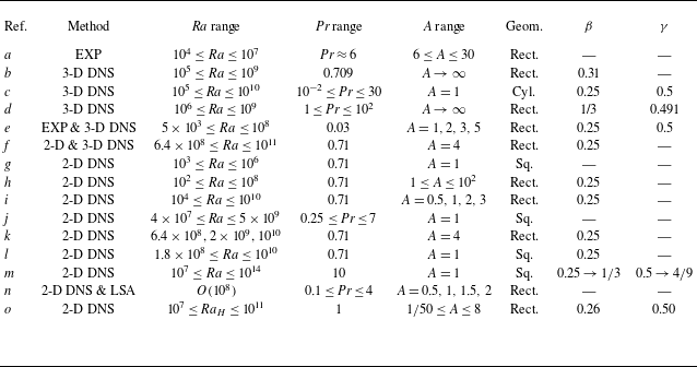
 Ra
 Pr
 A
 L
 H
 A=L/H
 A=D/H
 D
 H
 β
 γ
 Nu∼Raβ
 Re∼Raγ
 a
 b
 c
 d
 e
 f
 g
 h
 i
 j
 k
 l
 m
 n
 o
 b
 d
 A→∞
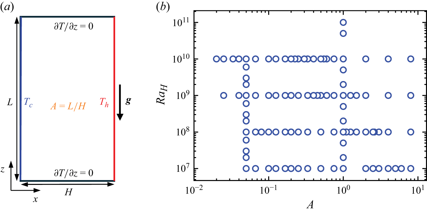
 a
 A=2
 RaH−A
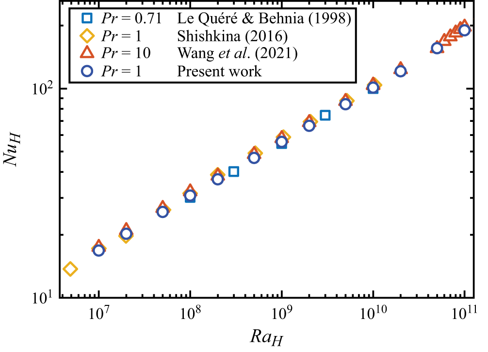
 NuH
 RaH
 A=1

 A=2
 RaH
 RaH=1×10⁷
 RaH=2×10⁷
 RaH=1×10⁸
 RaH=1×10⁹
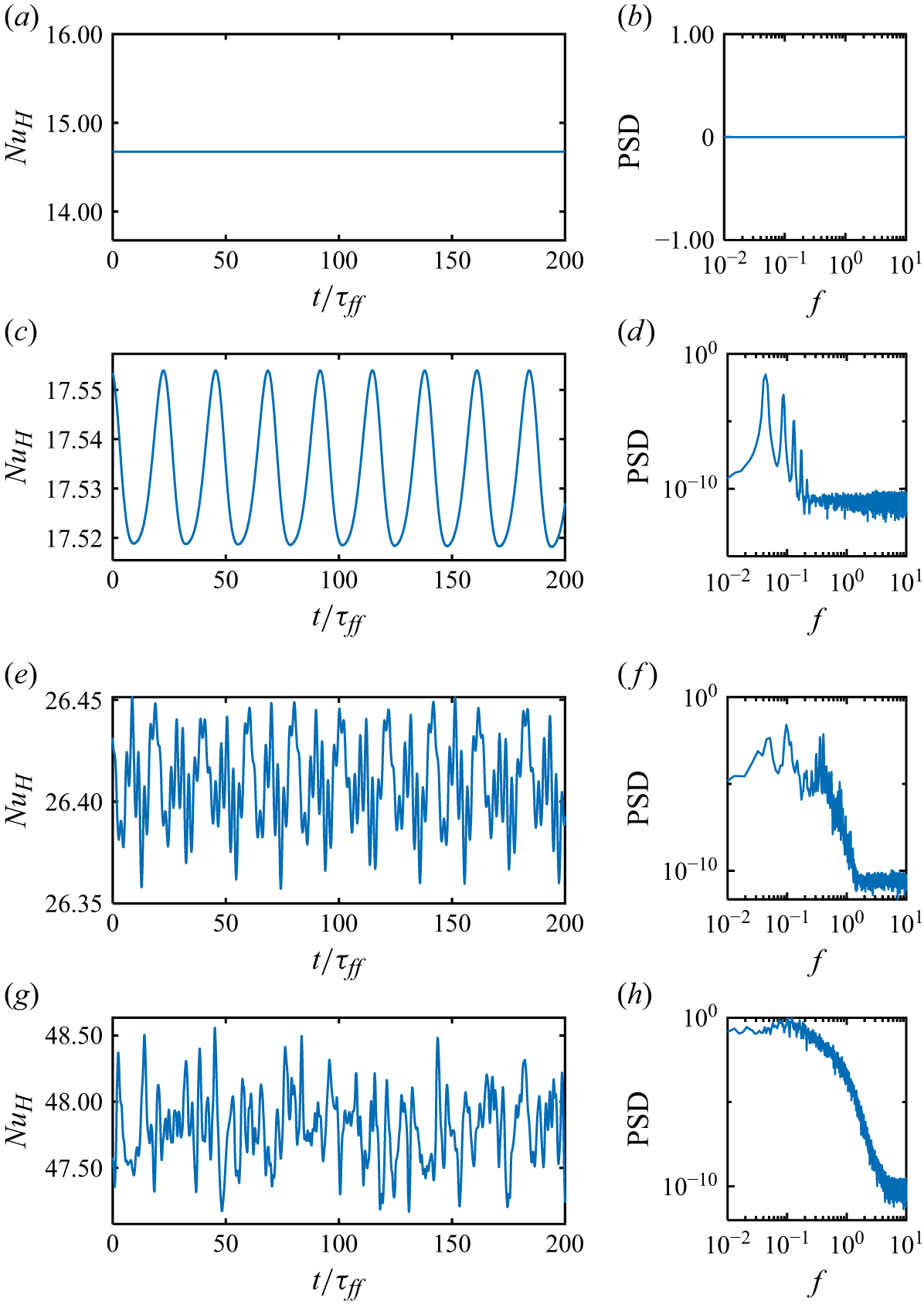
 NuH
 A=2
 RaH
 RaH=1×10⁷
 RaH=2×10⁷
 RaH=1×10⁸
 RaH=1×10⁹

 NuH
 A
 RaH=1×10⁹
 A=1/10
 A=1/2
 A=1
 A=8
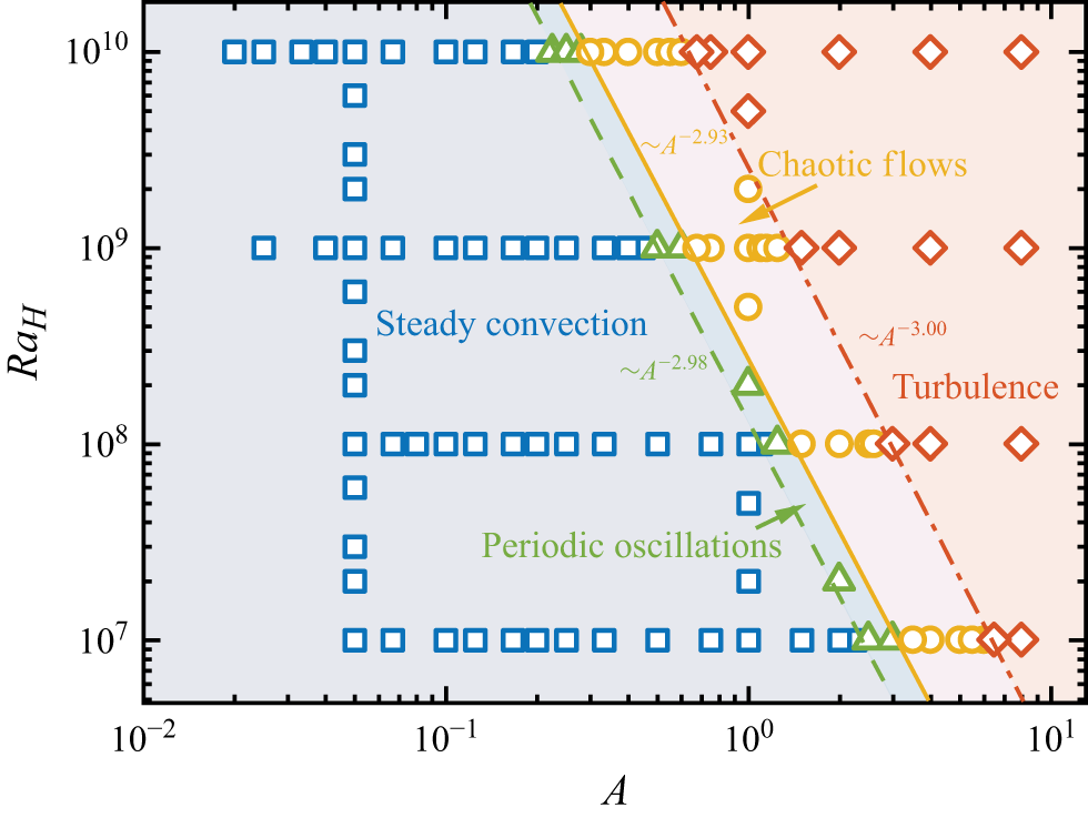
 RaH
 A
 RaH,c∼A−n
 n≃2.98±0.03
 n≃2.93±0.01
 n≃3.00±0.01
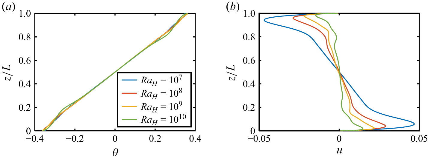
 θ(z/L)
 u(z/L)
 x/H=0.5
 RaH
 A=1
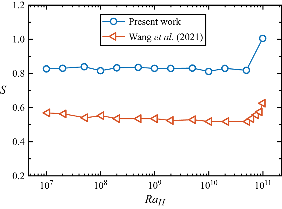
 S
 RaH
 Pr=10
 A=1
 Pr=1
 A=1
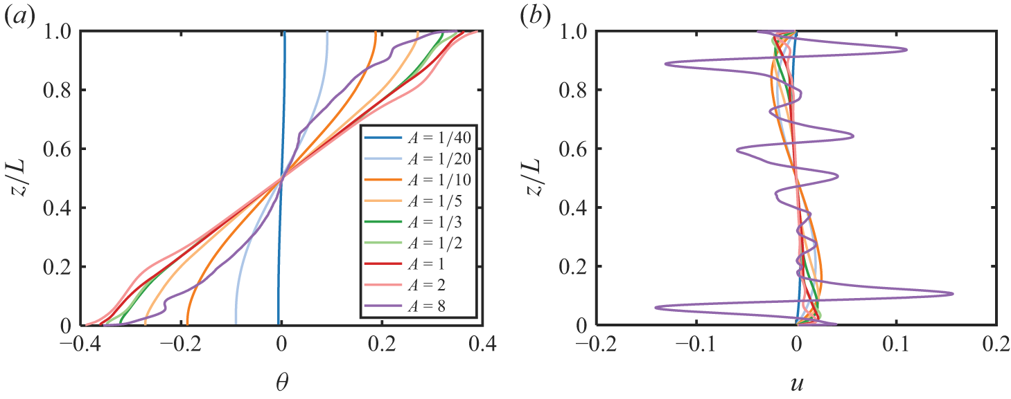
 θ(z/L)
 u(z/L)
 x/H=0.5
 A
 RaH=109

 S
 A
 RaH

 NuH
 A
 RaH
 A=1
 NuH/NuH(A=1)
 A
 Aopt
 Nuopt
 Nuopt
 NuH(A=1)
 RaH
 Nuopt/NuH(A=1)=0.59RaH0.04±0.01
 Aopt
 RaH
 Aopt=14.64RaH−0.21±0.01

 NuH/Nuopt
 A/Aopt
 RaH

 ReH
 A
 RaH
 RaH
 Ac
 RaH
 Ac=6.68RaH−0.22±0.01
 ReH/ReH(Ac)
 A/Ac
 RaH
 ReH/ReH(Ac)=1.13(A/Ac)2.36±0.13
 A/Ac<1
 ReH/ReH(Ac)=1.25(A/Ac)0.51±0.01
 A/Ac>1

 wmax/umax
 A
 L
 RaL
 RaH

 NuH
 RaH
 A
 A=1
 NuH=0.26RaH0.26±0.01
 NuHRaH−0.26
 RaH
 A=1
 Pr=0.71
 A=1
 Pr=1
 A=1
 Pr=10
 A→∞
 Pr=1

 L
 NuL
 RaL
 A
 NuL=0.16RaL0.28±0.01
 RaL≳106
 NuLRaL−0.28
 RaL

 ReH
 RaH
 A
 A=1
 ReH=0.24RaH0.50±0.01
 ReHRaH−0.50
 RaH

 L
 ReL
 RaL
 A
 ReL=0.30RaL0.49±0.01
 ReL/RaL0.49
 RaL

 RaL−A
 RaL,c∼An
 n≃0.02±0.03
 n≃0.07±0.01
 n≃0.00±0.01

 Pr=1
 H
 L
 H
 L
 A
 A=L/H
 RaH
 RaL
 H
 L
 Nx×Nz
 Δmax/ηK
 ηK
 ηK=(ν3/ϵu)1/4
 ν
 ϵu
 nBL
 t
 NuH
 NuL
 H
 L
 Nuϵθ
 ReH,ReL
 wmax
 H
 L



