1. Introduction
Thermal convection plays a critical role in various fields, including meteorology (Tong et al. Reference Tong, Chen and Malkawi2017), astrophysics (Pandey et al. Reference Pandey, Schumacher and Sreenivasan2021) and engineering (Huang et al. Reference Huang and Wu2024). Rayleigh–Bénard convection (RBC), a system in which a fluid is heated from below and cooled from above, serves as a classical configuration for studying thermal convection behaviour (see Lohse & Shishkina (Reference Lohse and Shishkina2024)) and Lohse & Xia (Reference Lohse and Xia2010)) for reviews). Typically, standard RBC (OB-RBC) is described by the Oberbeck–Boussinesq (OB) approximation, which relies on the following assumptions.
(OB1) Constant properties: the fluid’s viscosity
 $\mu$
, thermal conductivity
 $\lambda$
, specific heat capacity at constant pressure
 $c_p$
and isobaric expansion coefficient
 $\beta$
are constants.
(OB2) Incompressibility: the fluid is assumed to be incompressible, with buoyancy difference due to density variations being considered.
(OB3) Linear density–temperature relation: the density in the gravity term varies linearly with temperature, following the relationship:
 $\rho = \rho _{{m}} - \rho _{{m}} \beta (T- T_{{m}})$
. Here,
 $\rho$
is the density,
 $T$
is the temperature and
 $\rho _{{m}}$
and
 $T_{{m}}$
are the mean density and temperature, respectively.
However, real fluids are compressible and their properties vary with temperature and pressure. In many natural and industrial systems, substantial temperature and pressure differences cause the OB approximation to break down. This limitation has motivated extensive research into non-Oberbeck–Boussinesq (NOB) effects in RBC (Wan et al. Reference Wan, Wang, Wang, Xia, Zhou and Sun2020).
NOB effects can be categorised into two distinct types (Wan et al. Reference Wan, Wang, Wang, Xia, Zhou and Sun2020). The first type, referred to as NOB-I, involves the temperature-dependent variations in the fluid’s physical properties. Under NOB-I conditions, the assumptions OB1 and OB3 no longer hold. Research on NOB-I effects has primarily concentrated on two key parameters: the mean temperature of the centre plane (
 $T_{{c}}$
) and the Nusselt number (
 $Nu$
) (Yik et al. Reference Yik, Valori and Weiss2020). The mean temperature of the centre plane
 $T_{{c}}$
indicates temperature symmetry, while the Nusselt number
 $Nu$
reflects heat transfer efficiency. Wu & Libchaber (Reference Wu and Libchaber1991) conducted pioneering experimental studies on RBC in low-temperature helium and were the first to observe symmetry breaking in the temperature field. They discovered that under NOB-I conditions,
 $T_{{c}}$
in helium is greater than
 $T_{{m}}$
. Later, Zhang et al. (Reference Zhang, Childress and Libchaber1997) extended this investigation to glycerol, demonstrating that
 $T_{{c}}$
is also higher than
 $T_{{m}}$
in glycerol. Subsequent experimental and numerical studies have explored NOB-I effects in other common fluids, such as water (Ahlers et al. Reference Ahlers, Brown, Araujo, Funfschilling, Grossmann and Lohse2006; Sugiyama et al. Reference Sugiyama, Calzavarini, Grossmann and Lohse2009; Demou & Grigoriadis Reference Demou and Grigoriadis2019) and air (Wan et al. Reference Wan, Wang, Wang, Xia, Zhou and Sun2020; Pan & Choi Reference Pan and Choi2023, Reference Pan and Choi2024). These studies consistently found that
 $T_{{c}}$
is higher than
 $T_{{m}}$
in both water and air. Moreover, it was observed that
 $Nu$
slightly decreases in water under NOB-I conditions, while NOB-I effects have a negligible impact on
 $Nu$
in air.
Due to the drastic changes in the physical properties of supercritical fluids near the critical isochore, many researchers have explored the impact of NOB-I effects in supercritical fluids. Ahlers et al. (Reference Ahlers, Calzavarini, Araujo, Funfschilling, Grossmann, Lohse and Sugiyama2008, Reference Ahlers, Araujo, Funfschilling, Grossmann and Lohse2007) experimentally investigated the NOB-I effects of ethane near its critical isochore. They observed that
 $T_{{c}}$
is lower than
 $T_{{m}}$
in the gas-like region, while the opposite is true in the liquid-like region. Additionally, their findings revealed that NOB-I effects lead to an increase in
 $Nu$
in both regions, indicating heat transfer enhancement. Yik et al. (Reference Yik, Valori and Weiss2020) further experimentally studied the NOB-I effects in supercritical
 $\mathrm {SF}_6$
. In their study, they carefully controlled the Rayleigh (
 $Ra$
) and Prandtl (
 $Pr$
) numbers to independently regulate the intensity of NOB-I effects. Their results aligned with those of Ahlers et al. (Reference Ahlers, Calzavarini, Araujo, Funfschilling, Grossmann, Lohse and Sugiyama2008, Reference Ahlers, Araujo, Funfschilling, Grossmann and Lohse2007), confirming that
 $T_{{c}}$
is lower than
 $T_{{m}}$
in the gas-like region and higher in the liquid-like region. Additionally, they observed heat transfer enhancement up to 112 %. It is important to note that, although supercritical fluids exhibit high compressibility near the critical isochore, these researchers made significant efforts to minimise the effects of compressibility in their analyses of NOB-I effects.
The second type of NOB (NOB-II) effects focus on the impact of fluid compressibility. Under NOB-II conditions, OB2 and OB3 are no longer satisfied. In compressible fluids, density varies with both temperature and pressure, leading to two unique phenomena: the piston effect and the adiabatic temperature gradient (ATG). The piston effect, an efficient heat transfer mechanism driven by compression waves (Zappoli et al. Reference Zappoli, Bailly, Garrabos, Le Neindre, Guenoun and Beysens1990), can induce the oscillations in wall temperature near the onset of RBC, which has attracted significant scholarly attention (Amiroudine et al. Reference Amiroudine, Bontoux, LarroudÉ, Gilly and Zappoli2001; Chiwata & Onuki Reference Chiwata and Onuki2001; Kogan & Meyer Reference Kogan and Meyer2001; Amiroudine & Zappoli Reference Amiroudine and Zappoli2003; Bouafia & Daube Reference Bouafia and Daube2021). ATG refers to the additional temperature gradient required to trigger RBC under NOB-II conditions. This concept was first introduced by Giterman & Shteinberg (Reference Giterman and Shteinberg1970) and has since been supported by numerous theoretical (Carlès & Ugurtas Reference Carlès and Ugurtas1999), experimental (Kogan et al. Reference Kogan, Murphy and Meyer1999; Kogan & Meyer Reference Kogan and Meyer2001) and numerical (Amiroudine et al. Reference Amiroudine, Bontoux, LarroudÉ, Gilly and Zappoli2001; Accary et al. Reference Accary, Bontoux and Zappoli2005; Bouafia & Daube Reference Bouafia and Daube2021) studies.
Researchers have also focused on the scaling law of
 $Nu{-}Ra$
under NOB-II conditions. Ashkenazi & Steinberg (Reference Ashkenazi and Steinberg1999) conducted an experimental study on the turbulent convective behaviour of
 $\mathrm {SF}_6$
near the critical isochore at high
 $Ra$
(up to
 $5 \times 10^{14}$
), while exploring
 $Pr$
range from 1 to 100. They found that
 $Nu$
follow the scaling relationship
 $Nu \propto Ra^{0.3} Pr^{-0.2}$
. To further understand how NOB-II effects influence the scaling law of
 $Nu{-}Ra$
, Kogan & Meyer (Reference Kogan and Meyer2001) experimentally investigated the RBC of
 $^3\mathrm {He}$
near its critical isochore. They introduced a corrected Nusselt number (
 $Nu_{{corr}}$
) accounting for ATG. The results show that the convection current based on
 $Nu_{{corr}}$
versus the reduced Rayleigh number collapse onto a single curve in steady convective states (Kogan et al. Reference Kogan, Murphy and Meyer1999; Kogan & Meyer Reference Kogan and Meyer2001). In the turbulent regime, their findings (Kogan & Meyer Reference Kogan and Meyer2001) indicated that
 $Nu_{{corr}}$
and
 $Ra$
follow a 2/7 power law,
 $Nu \propto Ra^{2/7}$
, within the range
 $10^5 \lt Ra \lt 10^7$
. This conclusion was further supported by Accary et al. (Reference Accary, Bontoux and Zappoli2009), who conducted three-dimensional (3-D) numerical simulations of RBC in a supercritical fluid described by the van der Waals equation of state.
Although previous studies have reported the impact of NOB-I effects on the temperature symmetry, it remains unclear whether NOB-II effects lead to similar symmetry breaking. Furthermore, while the scaling law of
 $Nu{-}Ra$
under NOB-II conditions has been investigated, a clear understanding of the role of NOB-II effects on heat transfer is still lacking. To address these gaps, advanced numerical methods are required.
Previous numerical methods have used various approximations to simplify the solution of the Navier–Stokes equations, such as acoustic filtering (Accary et al. Reference Accary, Bontoux and Zappoli2009; Shen & Zhang Reference Shen and Zhang2012) and anelastic approximation (Bouafia & Daube Reference Bouafia and Daube2021). These methods are insufficient for fully capturing the intricate details of RBC under NOB-II conditions. For example, Bouafia & Daube (Reference Bouafia and Daube2021) used a stratification density approach to simplify the solution of the density. This model is just ‘an extended Boussinesq approximation using a stratified density field’, as Bouafia & Daube (Reference Bouafia and Daube2021) stated. The lattice Boltzmann method (LBM), as a mesoscopic method, has great potential for modelling compressible fluids. It has been widely applied in fields such as multiphase flow (Li et al. Reference Li, Kang, Francois, He and Luo2015; Huang & Wu Reference Jiang, Xu and Zhou2016; Chen et al. Reference Chen, Ahmad, Deng, Cai and Zhao2022; Gong et al. Reference Gong, Hu and Cheng2024), porous media flow (Jiang et al. Reference Jiang, Xu and Zhou2021) and turbulent flow (Chen et al. Reference Chen, Kandasamy, Orszag, Shock, Succi and Yakhot2003). Moreover, this method provides a clear physical representation and can effectively reveal the underlying mechanisms of convective heat transfer. Therefore, LBM is employed in this study to investigate NOB-II effects. Moreover, following the previous research (Kogan et al. Reference Kogan, Murphy and Meyer1999; Kogan & Meyer Reference Kogan and Meyer2001; Ahlers et al. Reference Ahlers, Araujo, Funfschilling, Grossmann and Lohse2007, Reference Ahlers, Calzavarini, Araujo, Funfschilling, Grossmann, Lohse and Sugiyama2008; Accary et al. Reference Accary, Bontoux and Zappoli2009; Yik et al. Reference Yik, Valori and Weiss2020; Bouafia & Daube Reference Bouafia and Daube2021), a supercritical fluid is selected for study due to its high compressibility near the critical isochore.
In this work, we present a lattice Boltzmann (LB) model capable of simulating supercritical fluids. The model is validated using the static cavity, Schwarzschild criterion and experimental data of Kogan et al. (Reference Kogan, Murphy and Meyer1999). Using this model, we perform LB simulations of RBC in supercritical fluids. Our results reveal that, unlike NOB-I effects, NOB-II effects do not cause symmetry breaking in temperature, density and momentum fields. However, due to density differences between the upper and lower regions, NOB-II effects break the symmetry of the velocity field. Moreover, NOB-II effects lead to the phenomenon of density inversion, wherein convection can still occur when the bottom fluid is denser than the top fluid. To our knowledge, this is the first report of density inversion in RBC. Additionally, we find that for a given
 $Ra$
, NOB-II effects have no impact on the
 $Re$
, while
 $Nu$
decreases linearly to 1 as NOB-II effects strengthen, indicating significant heat transfer deterioration (HTD).
The rest of the paper is organised as follows. In § 2, the details of the LB model are presented. Then, the model is validated in § 3 using the static cavity, Schwarzschild criterion and experimental data. The main results and discussions are presented in § 4. We first investigate the impact of NOB-II effects on the symmetry of the temperature, density and momentum fields. Then, we explore the phenomenon of density inversion and the mechanism behind it. Finally, we analyse the impact of NOB-II effects on heat transfer and reveal the mechanism behind HTD. In § 5, the main findings of this study are summarised and future research directions are discussed.
2. Numerical method
2.1. Lattice Boltzmann method
A lattice Boltzmann model consists of the following three parts: the evolution equation for the distribution function, the equilibrium distribution function and the discrete velocity model. Our model is developed based on the LB model proposed by Guo et al. (Reference Guo, Zheng and Shi2002), which incorporates the external force term. The evolution equation for the distribution function is given by
 \begin{align} f_i(\boldsymbol {x}+\boldsymbol {e_i}\delta _t,t+\delta _t) = f_i(\boldsymbol {x},t) -\frac {1}{\tau }\left (f_i-f_i^{{eq}}\right ) +\delta _t\left (1-\frac {1}{2\tau }\right )F_i, \end{align}
where
 $f_i$
is the distribution function,
 $\boldsymbol {x}$
is the position vector,
 $t$
is the time,
 $\delta _t$
is the time step and
 $\tau$
is the relaxation time, which is related to the kinematic viscosity
 $\nu$
:
 \begin{align} \tau =\frac {\nu }{c_s^2\delta _t}+\frac {1}{2}. \end{align}
Here,
 $c_s=c/\sqrt {3}$
is the sound speed and
 $c=\delta _x/\delta _t$
is the lattice speed. The equilibrium distribution function
 $f_i^{eq}$
is given by
 \begin{align} f_i^{{eq}}=w_i\rho \left [1+\frac {\boldsymbol {e_i\cdot u}}{c_s^2} +\frac {(\boldsymbol {e_i\cdot u})^2}{2c_s^4}-\frac {\boldsymbol {u\cdot u}}{2c_s^2}\right ], \end{align}
where
 $w_i$
is the weight coefficient,
 $\boldsymbol {u}$
is the velocity. We employ the D2Q9 discrete velocity model, which comprises nine discrete velocities. The nine discrete velocities are defined as follows (Qian et al. Reference Qian, d’Humières and Lallemand1992):
 \begin{align} \begin{matrix} \boldsymbol {e_i}=\begin{cases} (0,0), & i=0, \\ c\left ( \cos \left [ (i -1)\frac {\pi }{2} \right ] ,\sin \left [ (i -1)\frac {\pi }{2} \right ] \right ), & i=1{-}4, \\ \sqrt {2}c\left ( \cos \left [ (2i -1)\frac {\pi }{4} \right ] ,\sin \left [ (2i -1)\frac {\pi }{4} \right ] \right ) ,& i=5{-}8. \end{cases} \end{matrix} \end{align}
The corresponding weight coefficients are given by
 \begin{align} \begin{matrix} w_i=\begin{cases} 4/9, & i=0, \\ 1/9, & i=1{-}4, \\ 1/36, & i=5{-}8. \end{cases} \end{matrix} \end{align}
The macroscopic velocity
 $\boldsymbol {u}$
and density
 $\rho$
are calculated as follows:
 \begin{align} \rho \boldsymbol {u}=\sum _{i}f_i\boldsymbol {e_i}+\frac {\delta _t}{2}\boldsymbol {F}, \quad \rho =\sum _{i}f_i .\end{align}
The external force term
 $F_i$
in (2.1) is given by
 \begin{align} F_i=w _i\left [ \frac {\boldsymbol {e}_{\boldsymbol {i }}- \boldsymbol {u}}{c_{s}^{2}}+\frac {\left ( \boldsymbol {e_i\cdot u}\right ) \boldsymbol {e_i}} {c_{s}^{4}} \right ] \boldsymbol {\cdot F}. \end{align}
To make the LB model able to simulate supercritical fluids, we introduce the intermolecular forces proposed by Shan & Chen (Reference Shan and Chen1993, Reference Shan and Chen1994), defined as follows:
 \begin{align} \boldsymbol {F_{{m}}}(\boldsymbol {x})=- \frac {3}{\delta _t}G\psi (\boldsymbol {x})\sum _iw_i\psi (\boldsymbol {x}+ \boldsymbol {e_i}\delta _t)\boldsymbol {e_i} ,\end{align}
where
 $G$
is the interaction strength, which is set to
 $-$
1. At this point, the total force includes intermolecular forces and gravity:
 \begin{align} \boldsymbol {F}=\boldsymbol {F_{{m}}}+\boldsymbol {F}_{\boldsymbol g}=\boldsymbol {F_{{m}}}+\rho \boldsymbol {g}, \end{align}
where
 $\boldsymbol {g}$
is the acceleration due to gravity. The corresponding macroscopic equations can be derived from the Chapman–Enskog expansion (Guo et al. Reference Guo, Zheng and Shi2002).
Continuity equation:
 \begin{align} \frac {\partial \rho }{\partial t}+\boldsymbol {\nabla \cdot }(\rho \boldsymbol {u})=0 .\end{align}
Momentum equation:
 \begin{align} \frac {\partial (\rho \boldsymbol {u})}{\partial t}+\boldsymbol {\nabla \cdot }(\rho \boldsymbol {u}\boldsymbol {u})= -\boldsymbol {\nabla } p+\boldsymbol {\nabla \cdot } \left [\rho \nu (\boldsymbol {\nabla u} + \boldsymbol {\nabla u}^{\mathrm {T}})\right ] +\rho \boldsymbol {g} .\end{align}
Here,
 $p$
is the pressure, expressed in the following form (He & Doolen Reference He and Doolen2002):
 \begin{align} p=\rho c_s^2 +\frac {Gc^2}{2}\psi ^2 + O(\nabla ^2 \psi ). \end{align}
Therefore, to ensure that the
 $p{-}\rho {-}T$
relationship satisfies the given equation of state, the pseudopotential
 $\psi$
should take the following form:
 \begin{align} \psi (\boldsymbol {x})=\sqrt {\frac {2\left (p_{EOS}-\rho c_s^2\right )}{Gc^2}}, \end{align}
where
 $p_{EOS}$
is the pressure given by the equation of state.
2.2. Equation of state
In this study, we adopt the Peng–Robinson equation of state (Peng & Robinson Reference Peng and Robinson1976):
 \begin{eqnarray} p(T,\rho )=\frac {\rho RT}{1-b\rho }-\frac {a\varphi (T)\rho ^2}{1+2b\rho -b^2\rho ^2}, \end{eqnarray}
where
 \begin{align} \varphi (T)=\big [1+\big (0.37464+1.54226\omega -0.26992\omega ^2\big ) \big (1-\sqrt {T/T_{ {cr}}}\big )\big ]^2, \\[-27pt] \nonumber \end{align}
 \begin{align} a=0.45724 R^2T_{ {cr}}^2/p_{ {cr}}, \\[-24pt] \nonumber \end{align}
 \begin{align} b=0.0778 RT_{ {cr}}/{p_{ {cr}}} . \\[-6pt] \nonumber \end{align}
Here,
 $R$
represents the gas constant,
 $\omega$
is the acentric factor,
 $T$
denotes the temperature and ‘cr’ denotes the critical point properties. In this study, we use the values
 $a=2/49$
,
 $b=2/21$
,
 $R=1$
and
 $\omega =0.344$
, which are commonly employed to characterise the physical properties of water (Chen et al. Reference Chen, Ahmad, Deng, Cai and Zhao2022; Shah et al. Reference Shah, Jiang, Li, Chen, Liu, Gao, Ahmad, Zhao and Pan2023). From (2.16) and (2.17), the critical point physical properties can be obtained as
 $T_{ {cr}}=0.0778a/(0.45724bR)=0.07292$
and
 $p_{ {cr}}=0.0778^2 a / (0.45724b^2) = 0.05957$
. Substituting
 $T_{ {cr}}$
and
 $p_{ {cr}}$
into (2.14) yields the critical density
 $\rho _{ {cr}}=2.5419$
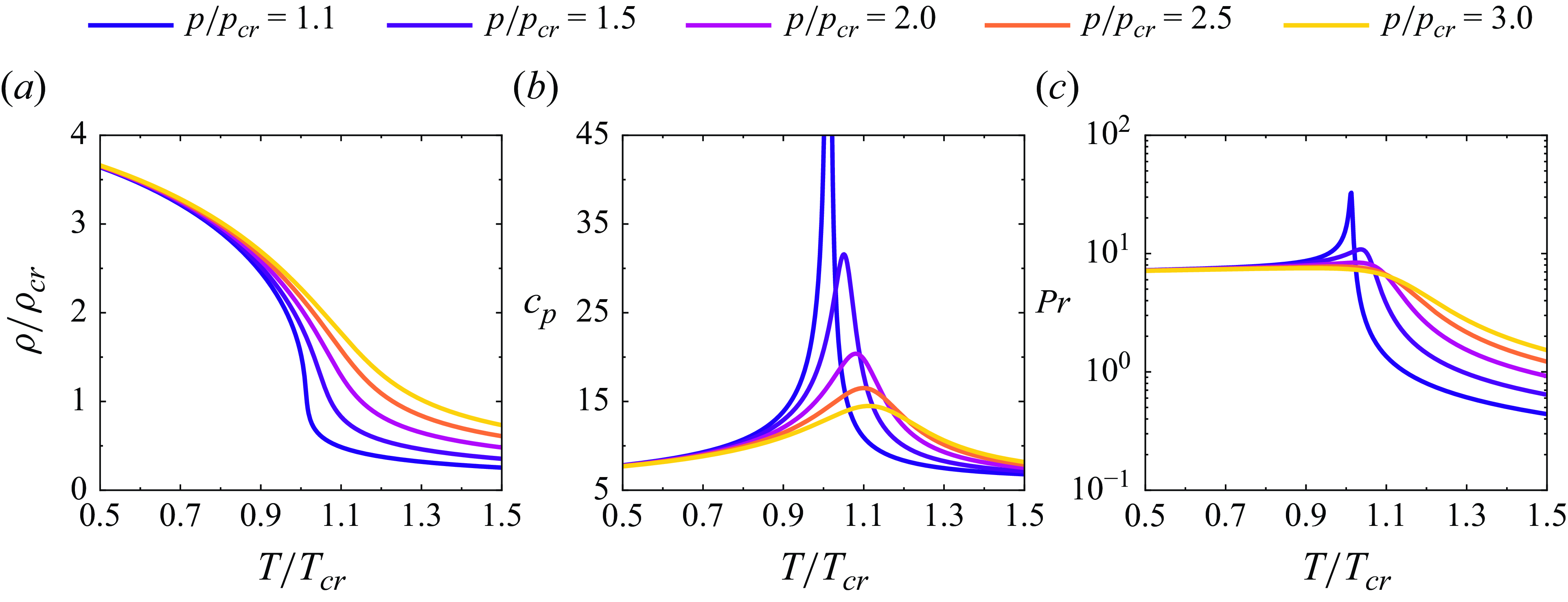
. Figure 1(a) shows the variation of density with temperature for various pressures. It can be seen that the density is drastically affected by pressure and temperature near its critical isochore.
Variation of (a) density
 $\rho$
, (b) specific heat at constant pressure
 $c_p$
and (c) Prandtl number
 $Pr$
with temperature for various pressures.

2.3. Energy equation
We adopt finite difference method to solve the energy equation, which can be expressed as follows (Moukalled et al. Reference Moukalled, Mangani and Darwish2016):
 \begin{align} \frac {\partial T}{\partial t}=-\boldsymbol {u \cdot \nabla } T+ \frac {1}{\rho c_{v}}\boldsymbol {\nabla \cdot }(\lambda \boldsymbol {\nabla } T) -\frac {T}{\rho c_{v}}\left (\frac {\partial p}{\partial T}\right )_{\rho } \boldsymbol {\nabla \cdot u} ,\end{align}
where
 $\lambda$
represents the thermal conductivity and
 $c_{v}$
is the specific heat at constant volume. The specific heat at constant pressure,
 $c_{p}$
, can be calculated using
 \begin{align} c_{p}=c_{v}-\frac {T}{\rho ^{2}} \left (\frac {\partial \rho }{\partial T}\right )_{p}\left (\frac {\partial p}{\partial T}\right )_{\rho }. \end{align}
Considering that LBM exhibits second-order accuracy in both time and space, we employ a second-order Runge–Kutta scheme for temporal discretization and a second-order central difference scheme for spatial discretisation. In this study, we focus on the effects of compressibility on RBC. Thus, we set
 $\nu$
,
 $c_v$
and
 $\lambda$
as constants with values 0.1, 5 and 1, respectively. Meanwhile, the gravity is set to
 $g=0.0001$
unless otherwise noted. Figures 1(b) and 1(c) show the variation of
 $c_p$
and
 $Pr=\rho c_p\nu /\lambda$
with temperature for various pressures, respectively.
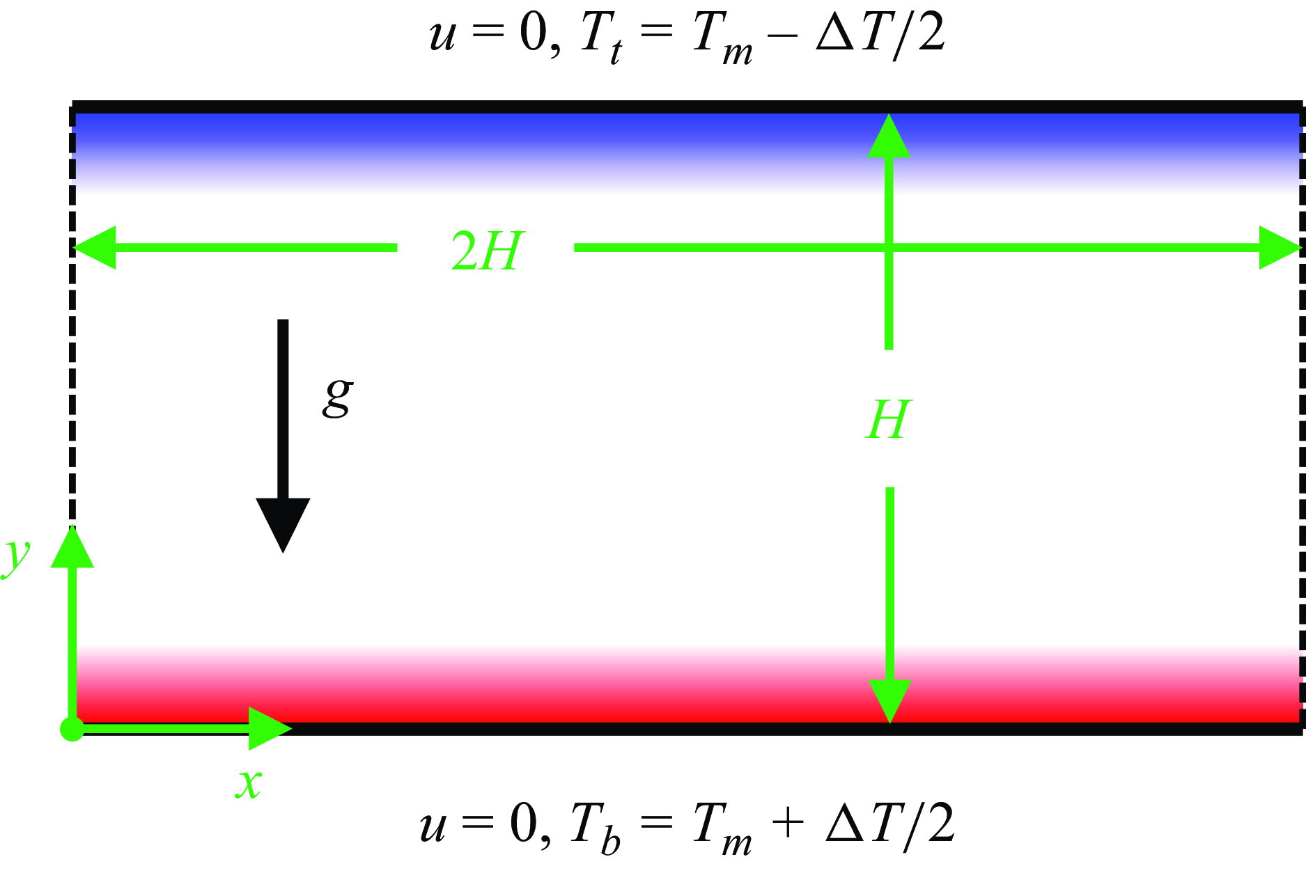
Schematic diagram of the flow configuration, where
 $H$
is the height of the RBC cell,
 $g$
is the acceleration due to gravity,
 $\Delta T$
is the temperature difference between the top and bottom plates,
 $T_{{m}}$
is the mean temperature, and
 $T_{ {t}}$
and
 $T_{ {b}}$
are the temperatures at the top and bottom plates, respectively. Solid lines represent the no-slip boundary conditions. Dashed lines represent the periodic boundary conditions.

2.4. Boundary conditions
Considering the roll period near the onset of RBC is
 $2.016H$
for an infinite aspect ratio (Clever & Busse Reference Clever and Busse1974; Shan Reference Shan1997), we selected a computational domain with an aspect ratio of 2, corresponding to a roll period of
 $2H$
. The schematic diagram of the flow configuration is shown in figure 2. Periodic boundary conditions were applied on the sides. This approach, with a roll period of
 $2H$
and periodic boundary conditions, is well established in the literature (Furukawa & Onuki Reference Furukawa and Onuki2002; Johnston & Doering Reference Johnston and Doering2009; Winchester et al. Reference Winchester, Howell and Dallas2022). The specific boundary conditions are as follows. The top and bottom plates are set as no-slip boundary conditions using Zou–He boundary scheme (Zou & He Reference Zou and He1997).
Top plate:
 \begin{align} f_4=f_2, \\[-28pt] \nonumber \end{align}
 \begin{align} f_7=f_5+\frac {\left ( f_1-f_3 \right )}{2}+\frac {\delta _t\left ( F_x+F_y \right )}{4}, \\[-28pt] \nonumber \end{align}
 \begin{align} f_8=f_6-\frac {\left ( f_1-f_3 \right )}{2}-\frac {\delta _t\left ( F_x-F_y \right )}{4}. \end{align}
Bottom plate:
 \begin{align} f_2=f_4, \\[-28pt] \nonumber \end{align}
 \begin{align} f_5=f_7-\frac {\left ( f_1-f_3 \right )}{2}-\frac {\delta _t\left ( F_x+F_y \right )}{4}, \\[-28pt] \nonumber \end{align}
 \begin{align} f_6=f_8+\frac {\left ( f_1-f_3 \right )}{2}+\frac {\delta _t\left ( F_x-F_y \right )}{4}. \end{align}
The top plate is maintained at a constant temperature
 $T_{{t}}=T_{{m}}-\Delta T/2$
, while the bottom plate is set at
 $T_{{b}}=T_{{m}}+\Delta T/2$
. At this point,
 $T_{{m}}$
is the arithmetic mean value of the top and bottom plates’ temperatures, and
 $\Delta T$
is the temperature difference between the top and bottom plates. Initially, both density and temperature are set to their mean values, with a temperature perturbation introduced at the centre of the domain. As shown in figure 1, fluid compressibility increases as the system approaches the critical point, leading to a corresponding rise in the peak of
 $ c_p$
. The stronger the compressibility, the more pronounced the NOB-II effects. However, the sharp fluctuation of
 $ c_p$
also introduces NOB-I effects. To emphasise NOB-II effects while minimising the impact of NOB-I effects, the computational conditions in this paper are set to
 $p_{{m}} = 2p_{ {cr}}$
and
 $T_{{m}} = 1.05T_{ {cr}}$
. The mean density
 $\rho _{{m}}$
is calculated by substituting
 $T_{{m}}$
and
 $p_{{m}}$
into (2.14).
3. Model validation
3.1. Static cavity
We constructed a static cavity configuration to validate the capability of our model in simulating fluid compressibility. The only difference between this configuration and RBC is that the temperatures of the top and bottom plates are reversed – i.e. the bottom plate is cooled, and the top plate is heated. This set-up ensures that the fluid remains stationary throughout the simulation. Under these conditions, the density and pressure profiles are governed by the following equations:
 \begin{align} \frac {\partial p}{\partial y}=\rho (p,T)g,\quad \frac {\partial p}{\partial x}=0 .\end{align}
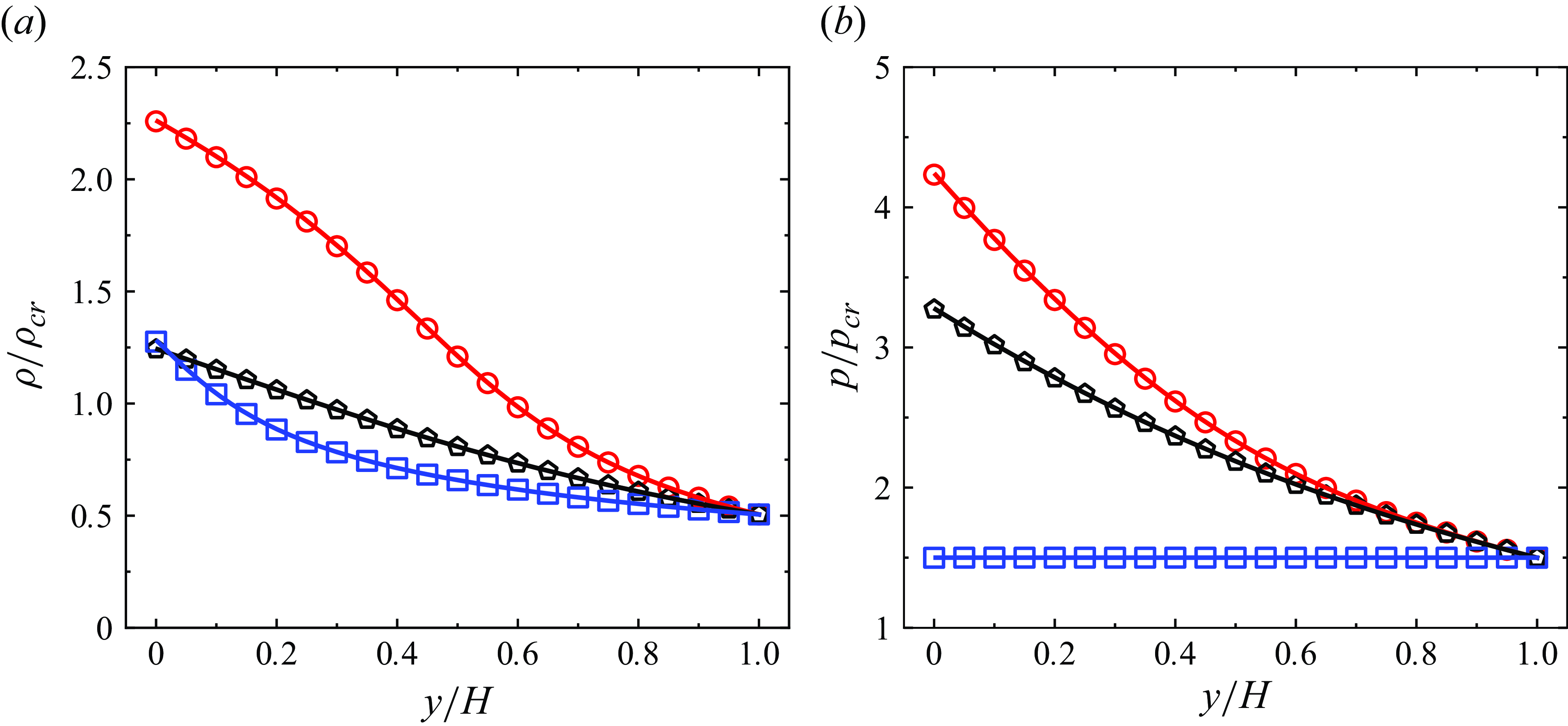
Figure 3 presents the density and pressure profiles of the static cavity under various conditions. Three simulation scenarios were set up: the first considers only the effect of gravity (black), the second considers only the effect of temperature (blue), and the third accounts for the effects of both temperature and gravity (red). The analytical solutions is obtained using the Euler method with a sufficiently small time step. The results demonstrate that the proposed model effectively captures the variation in density as a function of temperature and pressure. The computed results closely match the analytical solutions under all conditions, validating the model’s capability to accurately simulate fluid compressibility.
(a) Density and (b) pressure profiles of the static cavity under various conditions. Lines represent the analytical solutions. Points represent the calculated results using the presented LB model. In these cases, the cavity height is set to
 $H=200$
and the pressure of top plate is set to
 $p(H)=1.5p_{ {cr}}$
. Black lines and pentagon points represent the results for
 $T(y)=1.25T_{ {cr}}$
and
 $g=0.00025$
. Blue lines and square points represent the results for
 $T(y)=(1.05+0.2y/H)T_{ {cr}}$
and
 $g=0$
. Red lines and circle points represent the results for
 $T(y)=(1.05+0.2y/H)T_{ {cr}}$
and
 $g=0.00025$
.

3.2. Schwarzschild criterion
Giterman & Shteinberg (Reference Giterman and Shteinberg1970) proposed that the onset of RBC under NOB-II conditions should be determined using Schwarzschild criterion:
 \begin{align} Ra=\frac {\rho c_p g \beta H^4}{\lambda \nu }\left (\frac {\Delta T}{H}-\frac {\beta g T}{c_p}\right )\geqslant Ra_{{c}}, \end{align}
where
 $Ra_{{c}}$
is the critical Rayleigh number for the Schwarzschild criterion, which equals 1708 for both rigid boundaries (Carlès & Ugurtas Reference Carlès and Ugurtas1999). Based on this criterion, the temperature difference required for the onset of convection can be expressed as (Kogan et al. Reference Kogan, Murphy and Meyer1999)
 \begin{align} \Delta T_{ {on}}=\Delta T_{ {R}}+\Delta T_{ {ad}}=Ra_{{c}}\frac {\lambda \nu }{g\rho c_p\beta H^3}+\frac {gT\beta H}{c_p}. \end{align}
The first term on the right-hand side represents the contribution from the Rayleigh criterion and the second term accounts for the effect of ATG.
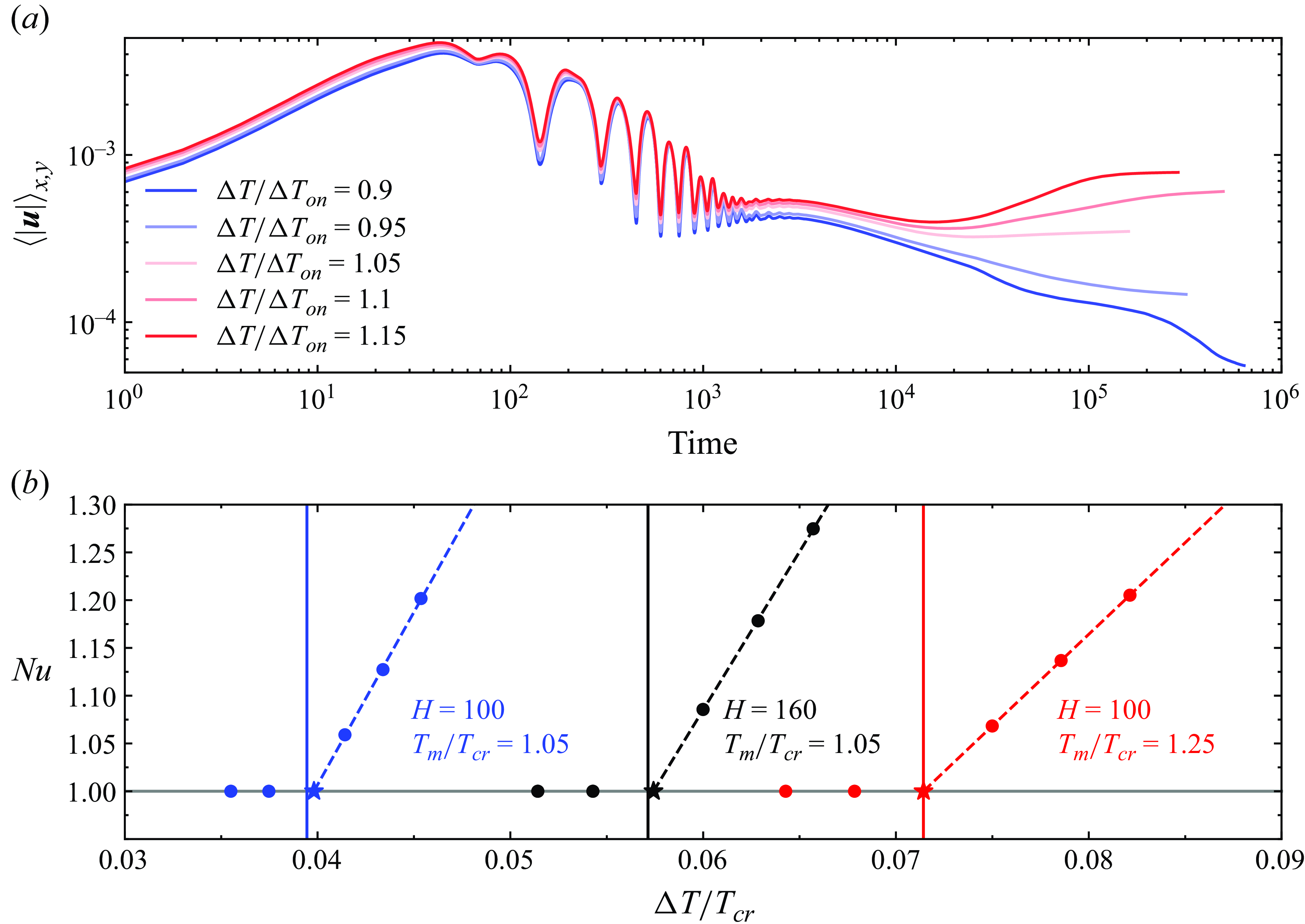
We use the proposed LB model to determine the onset temperature difference for convection and validate it by comparing it with the Schwarzschild criterion. First, we compute
 $\Delta T_{ {on}}$
according to the Schwarzschild criterion using (3.3). Then, we simulate the convective behaviour for
 $\Delta T$
values of 0.9
 $\Delta T_{ {on}}$
, 0.95
 $\Delta T_{on}$
, 1.05
 $\Delta T_{on}$
, 1.1
 $\Delta T_{on}$
and 1.15
 $\Delta T_{on}$
. Figure 4(a) illustrates the evolution of the spatial-averaged velocity
 $\langle |\boldsymbol {u}| \rangle _{x,y}$
over time. In the initial phase, similar oscillatory behaviour is observed across different
 $\Delta T$
due to the comparable nature of the introduced perturbations. However, when
 $\Delta T$
is less than
 $\Delta T_{on}$
,
 $\langle |\boldsymbol {u}| \rangle _{x,y}$
decreases steadily over time, indicating that convection initiated by the initial perturbation is unsustainable. At this point,
 $Nu$
is equal to 1, representing pure heat conduction. When
 $\Delta T$
exceeds
 $\Delta T_{on}$
,
 $\langle |\boldsymbol {u}| \rangle _{x,y}$
stabilises at a certain value over time, enabling sustained convection. Meanwhile, as shown in figure 4(a), the steady-state
 $\langle |\boldsymbol {u}| \rangle _{x,y}$
increases with
 $\Delta T$
, indicating that greater temperature differences lead to greater convective intensity. The convective onset temperature difference is obtained by linearly fitting and extrapolating the
 $Nu$
–
 $\Delta T$
relationship near the convective threshold (Yu et al. Reference Yu, Goldfaden, Flagstad and Scheel2017). As shown in figure 4(b), we fit a line through the points where
 $Nu \gt 1$
and the intersection of this line with
 $Nu = 1$
is taken as the onset point of convection determined by LBM. Here, the Nusselt number
 $Nu$
is defined as (Shishkina & Wagner Reference Shishkina and Wagner2016; Shishkina et al. Reference Shishkina and Wagner2016)
 \begin{align} Nu=-\frac {H}{\Delta T}\left \lt \frac {\partial T}{\partial y}\right \gt _{ {w}} ,\end{align}
where
 $\big \lt \cdot \big \gt _{ {w}}$
denotes the mean value over the top and bottom plates.
(a) Variation of the spatial-averaged velocity
 $\langle |\boldsymbol {u}| \rangle _{x,y}$
with time for various temperature difference
 $\Delta T$
at
 $H=60$
and
 $T_{{m}}=1.05T_{ {cr}}$
. (b) Variation of Nusselt number
 $Nu$
with temperature difference
 $\Delta T$
under various conditions. The same colour represents the same conditions and corresponding parameters have been specified in the figure. The vertical solid lines is the convective onset temperature difference
 $\Delta T_{ {on}}$
given by the Schwarzschild criterion. Five circle points under each condition represent the results calculated by LBM, from left to right the temperature difference is 0.9
 $\Delta T_{ {on}}$
, 0.95
 $\Delta T_{ {on}}$
, 1.05
 $\Delta T_{ {on}}$
, 1.1
 $\Delta T_{ {on}}$
and 1.15
 $\Delta T_{ {on}}$
. The dashed lines represent a linear fit to the last three points. Asterisk points represent the intersection of the dashed line with
 $Nu=1$
.

Effects of the (a–c) height
 $H$
and (d–f) mean temperature
 $T_{{m}}$
on the onset temperature difference. (a)
 $T_{{m}}=0.95T_{ {cr}}$
, (b)
 $T_{{m}}=1.05T_{ {cr}}$
, (c)
 $T_{{m}}=1.2T_{ {cr}}$
, (d)
 $H=50$
, (e)
 $H=100$
, (f)
 $H=150$
. Circle points represent the calculated results of LBM. Black solid lines represent
 $\Delta T_{ {on}}$
, which is obtained from the Schwarzschild criterion. Red dash-dotted lines represent
 $\Delta T_{ {ad}}$
. Blue dashed lines represent
 $\Delta T_{ {R}}$
.

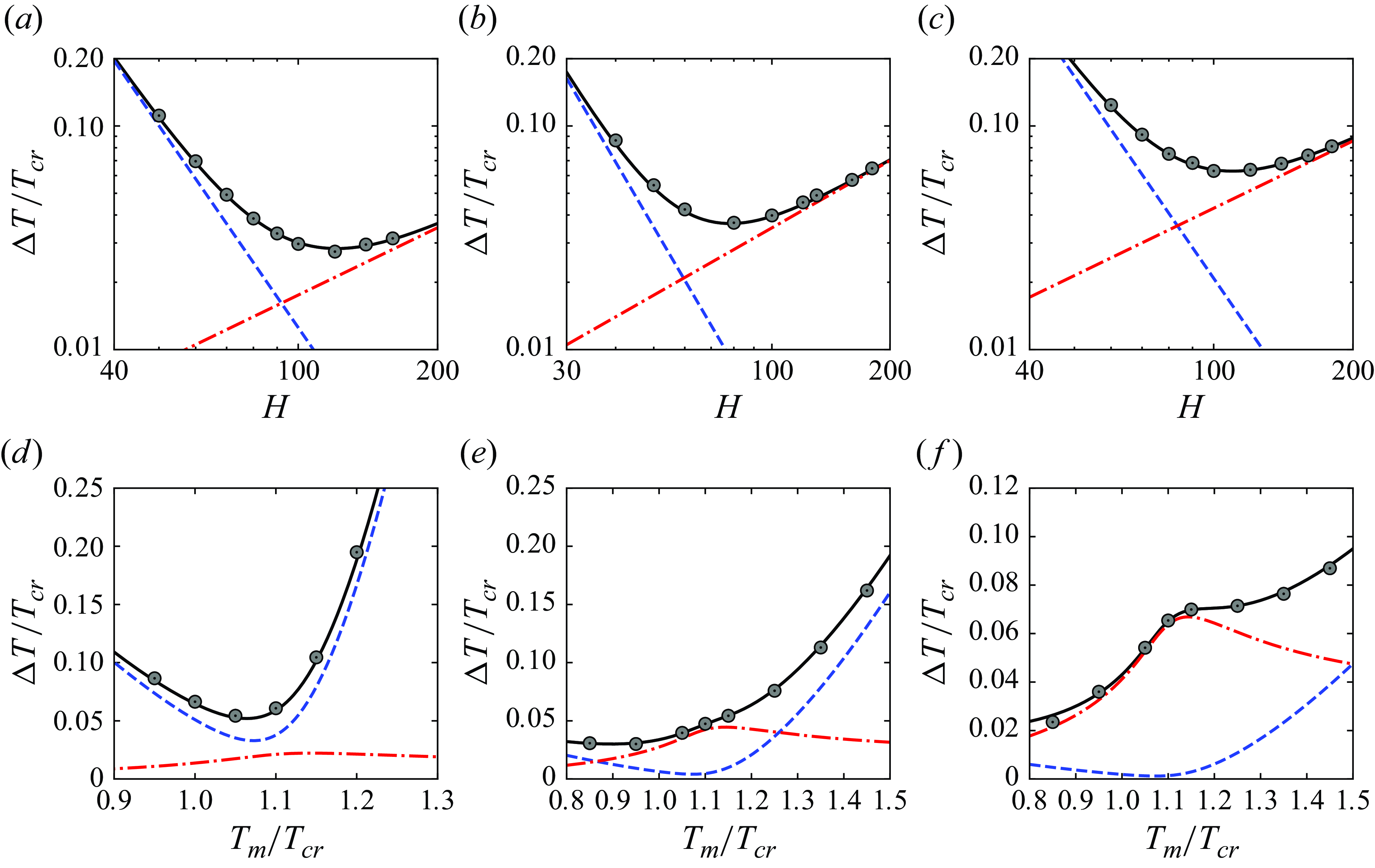
Figure 5 compares the calculated results with the Schwarzschild criterion. The points represent the onset temperature difference
 $\Delta T_{ {on}}$
obtained from the LB simulations, while the solid lines represent
 $\Delta T_{ {on}}$
given by the Schwarzschild criterion. It can be seen that the calculated results are in close agreement with the Schwarzschild criterion, further validating the accuracy of our numerical model. The relationship between
 $\Delta T_{ {on}}$
and
 $H$
for various
 $T_{{m}}$
is shown in figures 5(a)–5(c). When
 $H$
is small,
 $\Delta T_{ {R}}$
is the dominant factor, decreasing at a rate of
 $H^{-3}$
as
 $H$
increases. In contrast, for large
 $H$
,
 $\Delta T_{ {ad}}$
becomes the dominant factor, increasing linearly with
 $H$
. Thus, the onset temperature difference initially decreases and then increases as
 $H$
increases. Figures 5(d)–5(f) depict the variation of
 $\Delta T_{ {on}}$
with
 $T_{{m}}$
. The results show that
 $\Delta T_{ {R}}$
initially decreases and then increases as
 $T_{{m}}$
rises, reaching a minimum near the pseudo-critical point. This behaviour is primarily attributed to the peak in
 $c_p$
near the pseudo-critical point, as illustrated in figure 1(b). Conversely,
 $\Delta T_{ {ad}}$
increases and then gradually decreases as
 $T_{{m}}$
increases. The overall trend of
 $\Delta T_{ {on}}$
is governed by the combined effects of
 $\Delta T_{ {ad}}$
and
 $\Delta T_{ {R}}$
. When
 $H$
is small, the trend follows that of
 $\Delta T_{ {R}}$
, whereas for large
 $H$
, it aligns more closely with
 $\Delta T_{ {ad}}$
.
3.3. Experimental data
In this section, we further validate our model using experimental data. Kogan et al. (Reference Kogan, Murphy and Meyer1999) experimentally studied the RBC in supercritical
 $^3\mathrm {He}$
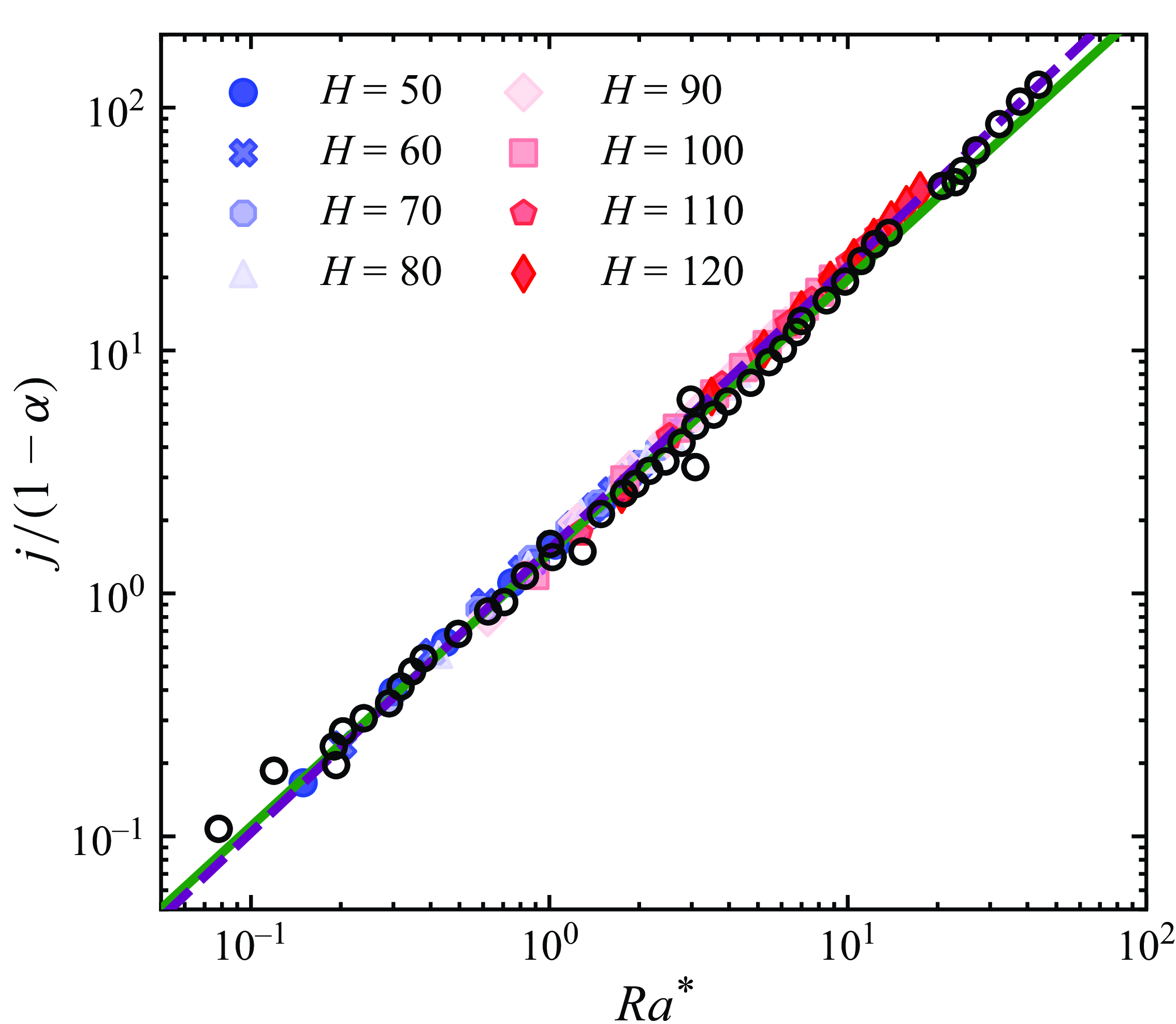
. Figure 6 presents the experimental results, where
 $Ra^*$
is defined as
 \begin{align} Ra^*=\frac {Ra-Ra_{{c}}}{Ra_{{c}}}. \end{align}
The results indicate that
 $j/(1-\alpha )$
follows a power-law relationship with
 $Ra^*$
, with the best power-law fit expressed as
 $j/(1-\alpha )=1.465 (Ra^* )^{1.125}$
. The definition of
 $j$
is given by (Kogan et al. Reference Kogan, Murphy and Meyer1999)
 \begin{align} j=(Nu-1)(Ra^* +1). \end{align}
The parameter
 $\alpha$
represents the ratio of
 $\Delta T_{ {ad}}$
to
 $\Delta T_{ {on}}$
, which can effectively indicate the intensity of NOB-II effects, as will be shown later. The value of
 $\alpha$
ranges from 0 to 1, where
 $\alpha =0$
corresponds to the standard RBC.
Figure 6 compares the best-fit curve from the experimental data with the results of LB simulations. The best power-law fit for the LB results is
 $j/(1-\alpha )=1.517 (Ra^* )^{1.116}$
. The results of the LB simulations are in good agreement with the experimental data. The strong agreement between the two further validates our numerical model. It is worth noting that the definitions of the horizontal and vertical axes in figure 6 differ from those used by Kogan et al. (Reference Kogan, Murphy and Meyer1999); however, they are equivalent, as demonstrated in Appendix A.
Comparation of the calculated results. The columns from left to right indicate the following: the Rayleigh number
 $Ra$
, the height of the RBC cell
 $H$
, the temperature difference
 $\Delta T$
, the ratio of adiabatic temperature gradient to the temperature difference
 $\alpha$
, the Nusselt number calculated by Clever & Busse (Reference Clever and Busse1974)
 $Nu_{ {C \& B}}$
, the Nusselt number calculated by the OB model
 $Nu_{{ob}}$
, the Nusselt number calculated by our model
 $Nu_{{nob}}$
, and the deviation between the results of the OB model and our model
 $Diff=(Nu_{{nob}}-Nu_{{ob}})/Nu_{{ob}}$
.

Variation of
 $j/(1-\alpha )$
with
 $Ra^*$
for various
 $H$
. Hollow points represent experimental data of Kogan et al. (Reference Kogan, Murphy and Meyer1999). Solid points are the calculated results of LBM for various
 $H$
. The green solid line,
 $j/(1-\alpha )=1.465(Ra^*)^{1.125}$
, is the best power-law fit to the experimental data. The purple dashed line,
 $j/(1-\alpha )=1.517(Ra^*)^{1.116}$
, is the best power-law fit to the results of LB simulations.

3.4. OB-RBC
The above comparisons validate the global parameters (e.g.
 $Nu$
,
 $\Delta T_{ {on}}$
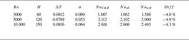
). To further assess the accuracy of our model, we compare the calculated flow fields under weak NOB-II effects with those obtained from OB-RBC. Table 1 presents a comparison of simulation parameters and results. In our simulations, we have used a value of
 $\alpha \approx 0.06$
to represent weak NOB-II effects. The results of OB-RBC are calculated using the thermal lattice Boltzmann method presented by Gao et al. (Reference Guo, Zheng and Shi2021) (denoted as OB model). The results show that the calculated results of OB-RBC closely align with the results reported by Clever & Busse (Reference Clever and Busse1974). The slight deviation observed in table 1 arises from the difference in
 $Pr$
. Clever & Busse (Reference Clever and Busse1974) set
 $Pr$
to 7.0, while in our calculations, we used a
 $Pr$
value of 8.25, which corresponds to supercritical fluid at
 $T_{{m}} = 1.05T_{ {cr}}$
and
 $p_{{m}} = 2p_{ {cr}}$
. Under the weak NOB-II effects, the Nusselt number (
 $ {Nu}$
) calculated by our model is slightly smaller than that obtained from OB-RBC, with a deviation within 5 %. This discrepancy is considered acceptable and further validates our model. The underlying reasons for this deviation will be discussed in detail in § 4.4.
(a,b) Normalised (a) temperature
 $\widetilde {T}$
and (b) reduced velocity
 $\widetilde {u}_y$
contours for
 $Ra=10\,000$
. Solid lines represent the results of the OB model. Dashed lines represent the results of our model. (c,d) Horizontal-averaged (c) temperature
 $\langle \widetilde {T} \rangle _x$
and (d) velocity
 $\langle \widetilde {u}_y \rangle _x$
profiles for various
 $Ra$
. Solid lines represent the results of our model. Points represent the results of the OB model.

For better comparison, we define the normalised temperature as follows:
 \begin{align} \widetilde {T}=\frac {T-T_{{m}}}{T_{ {b}}-T_{ {t}}}. \end{align}
The normalised temperature ranges from
 $-$
0.5 to 0.5, where the bottom plate is fixed at 0.5 and the top plate is fixed at
 $-$
0.5. The reduced velocity is defined as
 \begin{align} \widetilde {u}_y=\frac {u_y H\rho }{\nu \rho _{{m}}}. \end{align}
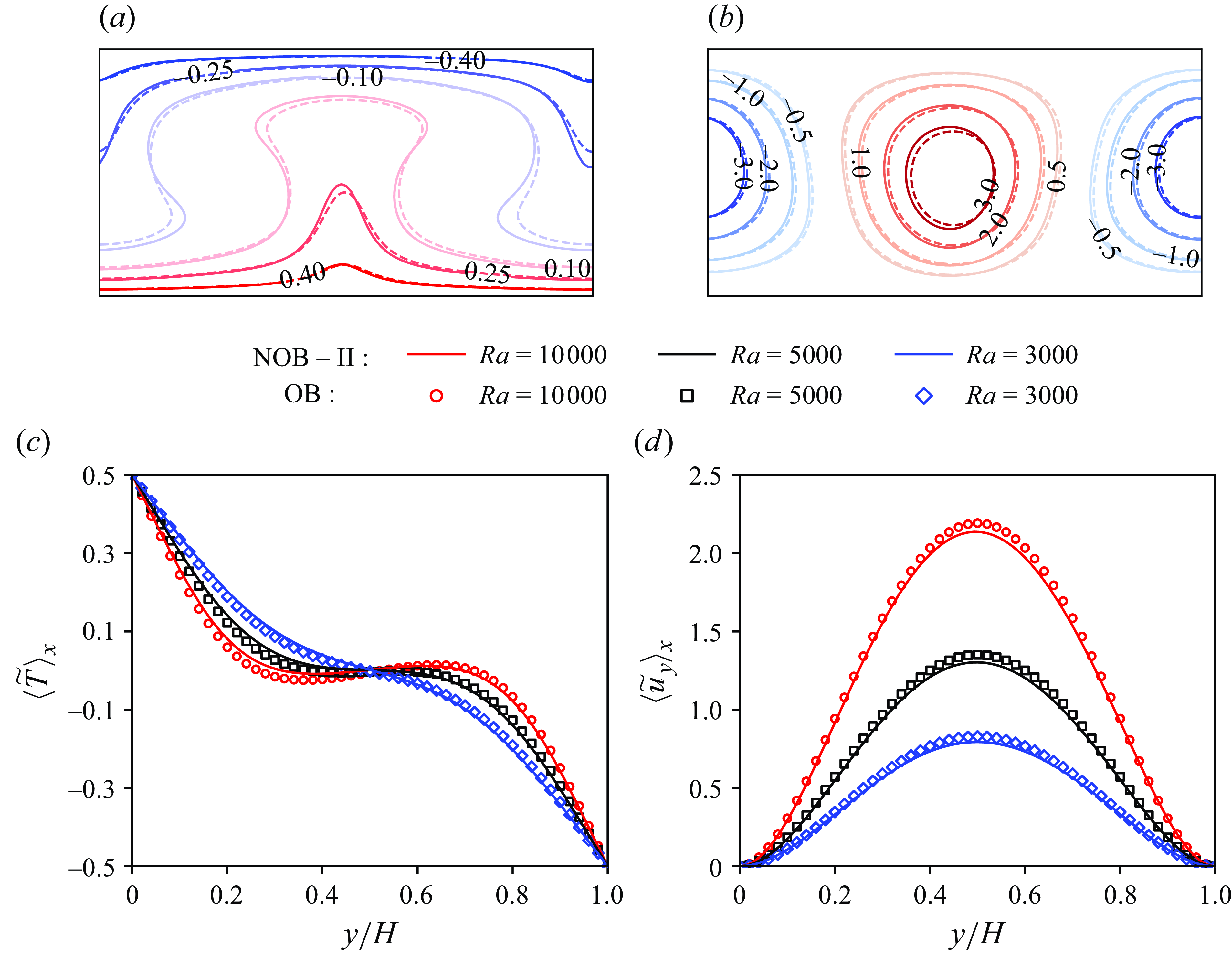
Figures 7(a) and 7(b) compare the flow fields obtained from the OB model with those from our model. It can be observed that the temperature and velocity fields calculated by our model under weak NOB-II effects show a strong agreement with those of the OB model. Figures 7(c) and 7(d) provide further comparison of the horizontal-averaged temperature and velocity profiles calculated by both models, with results again demonstrating good agreement. Overall, the calculations from our model are in close alignment with those of the OB model under weak NOB-II effects. The deviation induced by the NOB-II effect remains within an acceptable range, which serves to fully validate our model. The differences in the results of the two models due to the NOB-II effect will be discussed in detail in § 4.
4. Results and disscussion
4.1. Symmetry
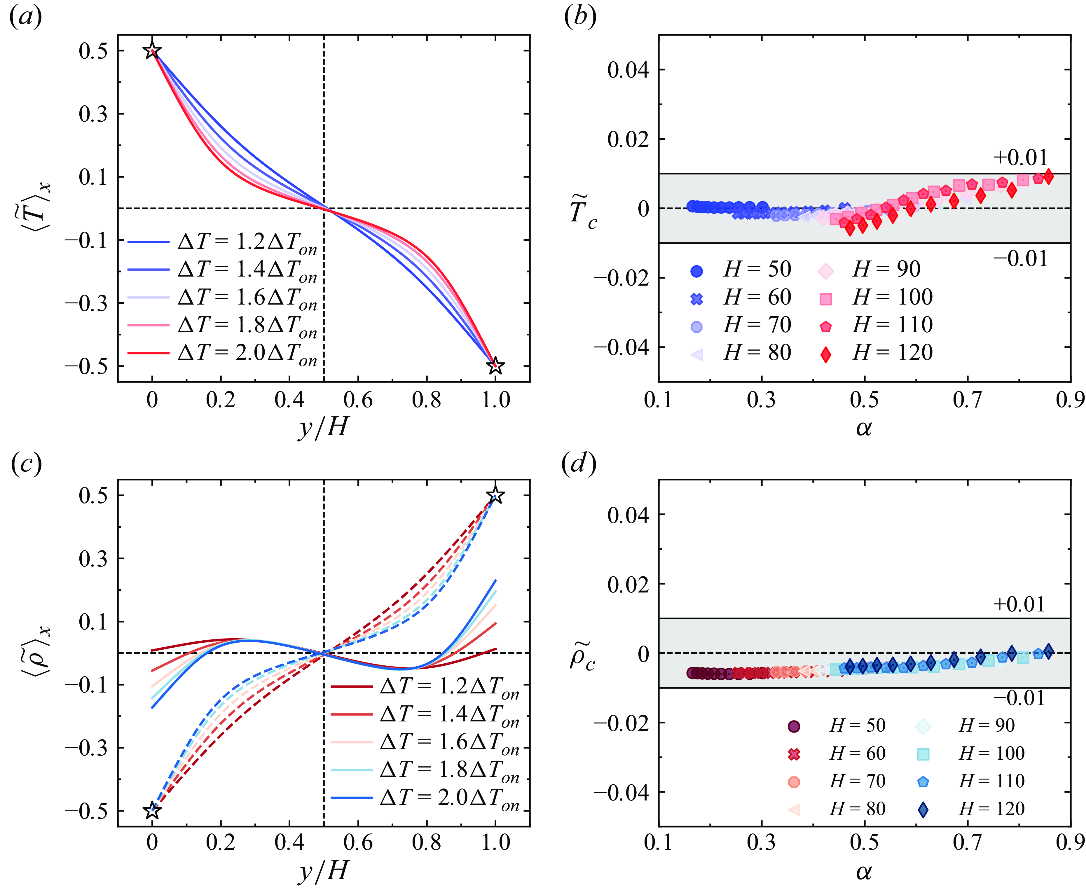
First, we examine whether NOB-II effects disrupt temperature symmetry in the same way as NOB-I effects. Figure 8(a) shows the horizontal-averaged normalised temperature,
 $\langle \widetilde {T} \rangle _x$
, as a function of
 $y/H$
for various temperature differences. The results indicate that the overall symmetry of the temperature profile remains intact. All curves pass through the point (0.5, 0) without significant deviation as the temperature difference increases. We further present the variation of the normalised mean temperature of central plane
 $\widetilde {T}_{{c}}$
with
 $\alpha$
in figure 8(b). The results show that
 $\widetilde {T}_{{c}}$
fluctuates within a narrow range of
 $\pm 0.01$
. Previous studies on the NOB-I effects have reported deviations in
 $\widetilde {T}_{{c}}$
as follows:
 $+0.05{-}+0.17$
for glycerol (Zhang et al. Reference Zhang, Childress and Libchaber1997),
 $0{-} +0.08$
for water (Ahlers et al. Reference Ahlers, Brown, Araujo, Funfschilling, Grossmann and Lohse2006; Sugiyama et al. Reference Sugiyama, Calzavarini, Grossmann and Lohse2009; Demou & Grigoriadis Reference Demou and Grigoriadis2019),
 $0{-} +0.05$
for air (Wan et al. Reference Wan, Wang, Wang, Xia, Zhou and Sun2020),
 $-0.22{-} +0.08$
for supercritical SF
 $_6$
(Yik et al. Reference Yik, Valori and Weiss2020) and
 $-0.035{-} +0.02$
for supercritical ethane (Ahlers et al. Reference Ahlers, Araujo, Funfschilling, Grossmann and Lohse2007, Reference Ahlers, Calzavarini, Araujo, Funfschilling, Grossmann, Lohse and Sugiyama2008). Additionally, these studies consistently show that the deviation increases with the intensity of NOB-I effects. In contrast, the deviations observed in figure 8(b) are minimal (<0.01) and show no clear trend. Therefore, we conclude that the NOB-II effects have no impact on
 $\widetilde {T}_{{c}}$
, meaning that NOB-II effects do not affect
 $\widetilde {T}_{{c}}$
and thus do not break the temperature symmetry. The slight fluctuations in
 $\widetilde {T}_{{c}}$
are most likely caused by minor variations in
 $c_p$
and
 $\beta$
with temperature (see figure 1), which are attributable to the NOB-I effects.
(a) Horizontal-averaged normalised temperature
 $\langle \widetilde {T} \rangle _x$
as a function of
 $y/H$
for various
 $\Delta T$
at
 $H=100$
. (b) Variation of the normalised temperature of centre plane
 $\widetilde {T}_{{c}}$
with
 $\alpha$
for various
 $H$
. (c) Horizontal-averaged normalised density
 $\langle \widetilde {\rho } \rangle _x$
as a function of
 $y/H$
for various
 $\Delta T$
at
 $H=100$
. Dashed lines represent the result of (4.2)
 $\widetilde {\rho } = -\widetilde {T}$
. (d) Variation of the normalised centre plane density
 $\widetilde {\rho }_{{c}}$
with
 $\alpha$
for various
 $H$
. Ten data points for each
 $H$
represent varying
 $\Delta T$
values, specifically from 1.1 to
 $2.0\Delta T_{ {on}}$
in increments.

Under OB and NOB-I conditions, the density in the buoyancy term decreases as temperature increases, maintaining a one-to-one correspondence. However, under NOB-II conditions, density is determined by both temperature and pressure, making the study of the density field particularly important (Amiroudine et al. Reference Amiroudine, Bontoux, LarroudÉ, Gilly and Zappoli2001; Carlès & El Khouri Reference Carlès and El Khouri2001). To examine the density symmetry, we define the normalised density as follows:
 \begin{align} \widetilde {\rho }=\frac {\rho -\rho _{{m}}}{\rho _{{m}} \beta \Delta T}, \end{align}
Under OB conditions,
 $\widetilde {\rho }$
and
 $\widetilde {T}$
are related by the following equation:
 \begin{align} \widetilde {\rho }=\frac {\rho -\rho _{{m}}}{\rho _{{m}} \beta \Delta T} =\frac {-\rho _{{m}}\beta (T-T_{{m}})}{\rho _{{m}}\beta (T_{ {b}}-T_{ {t}})} =-\widetilde {T} .\end{align}
This implies that
 $\widetilde {\rho }$
and
 $\widetilde {T}$
have opposite signs under OB conditions. Figure 8(c) shows the variation of the horizontal-averaged normalised density distribution
 $\langle \widetilde {\rho } \rangle _x$
with
 $y/H$
for various
 $\Delta T$
. The results indicate that the overall symmetry of the density profile remains intact. Figure 8(d) presents the variation of the normalised mean density at the centre plane
 $\widetilde {\rho }_{{c}}$
with
 $\alpha$
. The results show that
 $\widetilde {\rho }_{{c}}$
fluctuates within a narrow range of
 $\pm$
0.01, with deviations of less than 0.01. This suggests that NOB-II effects do not break the density symmetry either. However, the profiles in figure 8(c) deviate significantly from the relationship described by (4.2). Therefore, it is necessary to further investigate the distribution of the density field, which is discussed in detail in § 4.2.
While studying the symmetry of temperature and density, values at the centre plane are of primary interest. In contrast, when analysing the symmetry of velocity under NOB conditions, the focus shifts to the velocity difference between the upper and lower regions (Horn et al. Reference Horn, Shishkina and Wagner2013). Under OB conditions, the velocity field is symmetric along the centre plane. However, under NOB conditions, this symmetry is disrupted. Experimental studies on NOB-I effects have revealed asymmetries in the upper and lower velocity fields (Valori et al. Reference Valori, Elsinga, Rohde, Tummers, Westerweel and van der2017). Therefore, it is essential to investigate the impact of NOB-II effects on the velocity field.
(a) Variation of the horizontal-averaged absolute value of
 $u_y$
with
 $|y/H-0.5|$
for various
 $\Delta T$
at
 $H=100$
. Dashed lines represent the results for the lower region (
 $y/H\lt 0.5$
). Points represent the results for the upper region (
 $y/H\gt 0.5$
). (b) Variation of the velocity deviation
 $\varepsilon _u$
in the upper and lower regions with
 $|y/H-0.5|$
for various
 $\Delta T$
at
 $H=100$
. (c) Variation of the horizontal-averaged absolute value of
 $\rho u_y$
with
 $|y/H-0.5|$
for various
 $\Delta T$
at
 $H=100$
. (d) Variation of the momentum deviation
 $\varepsilon _{\rho u}$
in the upper and lower regions with
 $|y/H-0.5|$
for various
 $\Delta T$
at
 $H=100$
.

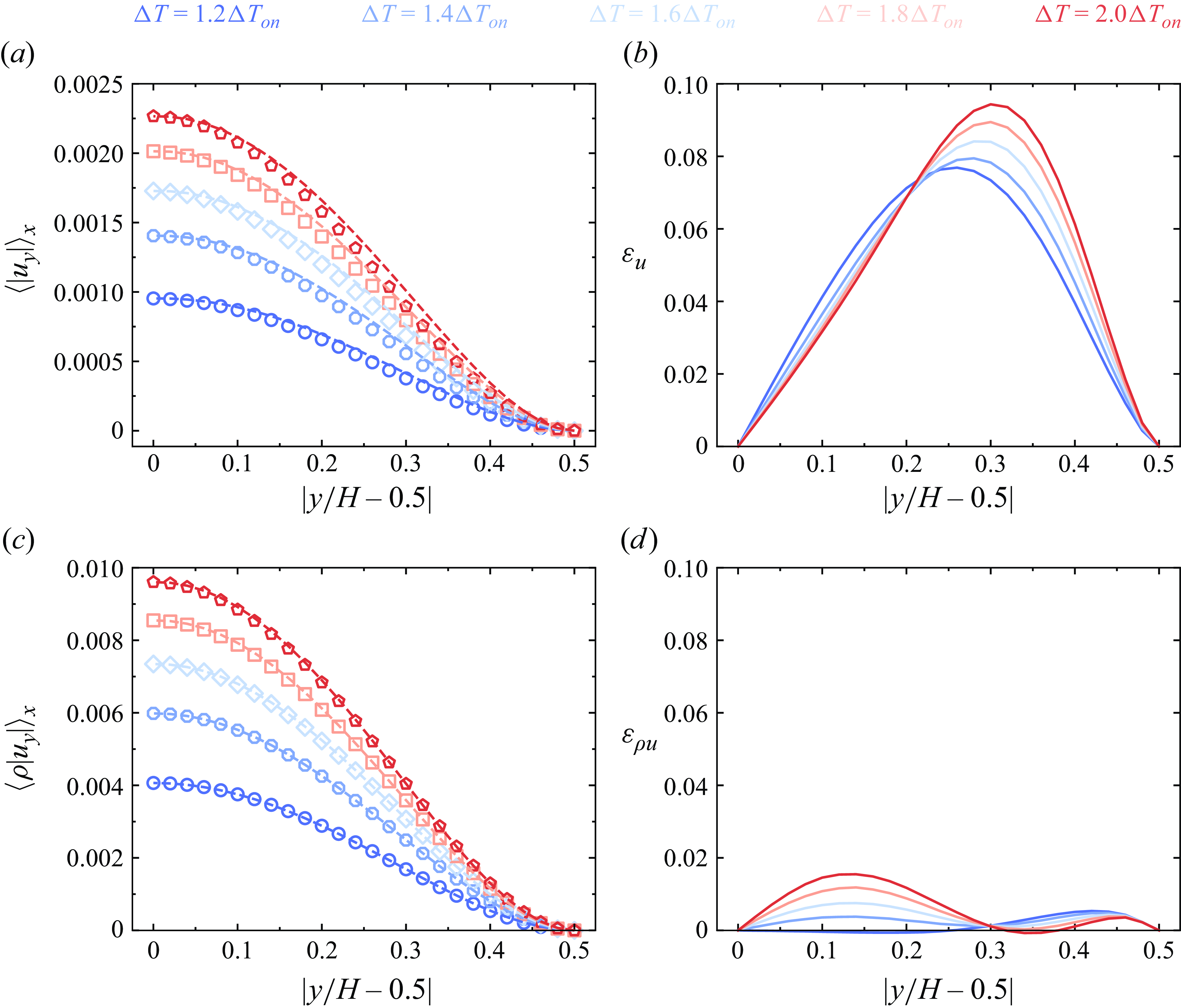
Figure 9(a) shows the variation of the horizontal-averaged absolute value of
 $u_y$
with
 $|y/H - 0.5|$
. Here, the horizontal coordinate is taken as
 $|y/H - 0.5|$
rather than
 $y/H$
to emphasise the asymmetry between the upper and lower regions. The results indicate that the velocity field is asymmetric along the central horizontal plane, with
 $\langle |u_y| \rangle _x$
in the lower region consistently smaller than in the upper region. The relative deviation
 $\varepsilon _u$
between the two regions is shown in figure 9(b), where
 $\varepsilon _u$
is defined as follows:
 \begin{align} \varepsilon _u = \frac {\langle |u_y| \rangle _{x,{upper}} - \langle |u_y| \rangle _{x,{lower}}} { \langle |u_y| \rangle _{x,y}}, \end{align}
with the subscripts ‘upper’ and ‘lower’ representing the upper and lower regions, respectively. Figure 9(b) shows that the deviation between the two regions increases and then decreases with
 $|y/H-0.5|$
and the maximum deviation increases with
 $\Delta T$
.
To further analyse the cause of this asymmetry, figure 9(c) presents the variation of the horizontal-averaged absolute value of
 $\rho u_y$
with
 $y$
. This figure shows that momentum symmetry between the upper and lower regions is maintained, with minimal differences observed between the two regions. Figure 9(d) displays the relative deviation
 $\varepsilon _{\rho u}$
, which is defined as follows:
 \begin{align} \varepsilon _{\rho u} = \frac {\langle |\rho u_y| \rangle _{x,{upper}} - \langle |\rho u_y| \rangle _{x,{lower}}} { \langle |\rho u_y| \rangle _{x,y}} .\end{align}
The results indicate that the momentum deviation remains within 0.02. In contrast, the maximum deviation in velocity is close to 0.1, as shown in figure 9(b). Thus, we conclude that under NOB-II conditions, the symmetry of momentum is preserved, while the asymmetry observed in the velocity field is attributed to variations in the density field.
4.2. Density inversion
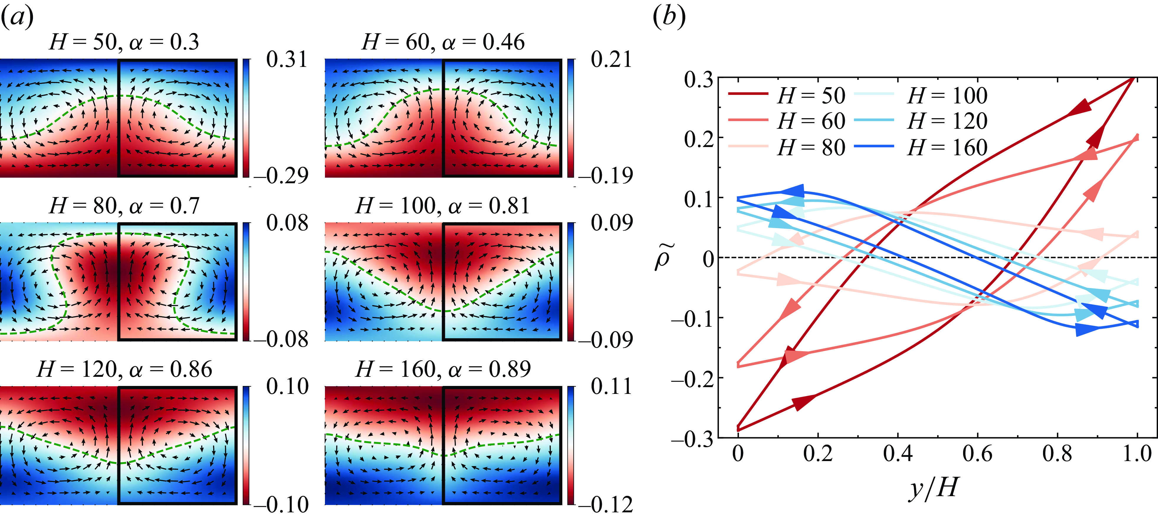
Figure 10(a) presents the normalised density
 $\widetilde {\rho }$
contours at
 $\Delta T = 1.1\Delta T_{ {on}}$
for various heights. In OB-RBC, it is widely accepted that the fluid at the bottom is less dense than at the top. Due to buoyancy, the lighter fluid rises, driving thermal convection. However, as
 $H$
increases, leading to stronger NOB-II effects, the density field exhibits an intriguing inversion. As shown in figure 10(a), when
 $\alpha \leq 0.7$
, the density remains higher at the top and lower at the bottom, consistent with OB-RBC behaviour. At this point, the contours for
 $\widetilde {\rho } = 0$
show a distribution of shapes that are convex upwards at the hot plume and concave downwards at the cold plume. However, when
 $\alpha \geqslant 0.81$
, an inversion in the density field occurs, with the density becoming lower at the top and higher at the bottom. At this point, the contours for
 $\widetilde {\rho } = 0$
display shapes that are concave downwards in the hot plume and convex upwards in the cold plume.
We now examine the mechanism of density inversion, using hot plumes as a representative case (a similar analysis applies to cold plumes). Generally, density decreases with increasing temperature and increases with rising pressure. Due to fluid compressibility, the effect of pressure cannot be neglected. Although the fluid at the bottom is hotter, it is also subjected to higher pressure. As the hot plume ascends, its temperature decreases, which would typically increase its density. Simultaneously, the pressure also decreases, which tends to lower its density. When both the pressure gradient and fluid compressibility are significant, the effect of pressure on density outweighs the effect of temperature. Consequently, the density gradually decreases as the hot plume rises, leading to the phenomenon of density inversion.
Although the mechanism of density inversion is understood, it remains unclear how convection can persist when density inversion occurs. This is particularly intriguing, as it is generally accepted that a fluid is stable when its density increases with height. A typical example of this is the stable conduction stratification of penetrative RBC (Toppaladoddi & Wettlaufer Reference Toppaladoddi and Wettlaufer2018; Wang et al. Reference Wang, Zhou, Wan and Sun2019). To elucidate the mechanism of convection, figure 10(b) shows the normalised density distribution along the flow circulation lines (indicated by the solid lines in figure 10
a). As shown in figure 10(b), the fluid density decreases with increasing height when
 $H$
is large, further confirming the occurrence of density inversion. From figure 10(b), we observe a common feature in the density circulation lines: for all values of
 $H$
, the fluid exhibits counterclockwise circulation on the
 $\rho$
–
 $y/H$
plot. This implies that, for a given
 $y$
, the density of the rising hot plume is always lower than that of the sinking cold plume.
(a) Normalised density
 $\widetilde {\rho }$
contours at
 $\Delta T = 1.1\Delta T_{ {on}}$
for various heights. Black arrows represent velocity vectors. The green dashed lines represent
 $\widetilde {\rho }=0$
. (b) Normalised density
 $\widetilde {\rho }$
distribution on the circulation lines (solid lines in panel a) for various heights.The arrows represent the direction of flow.

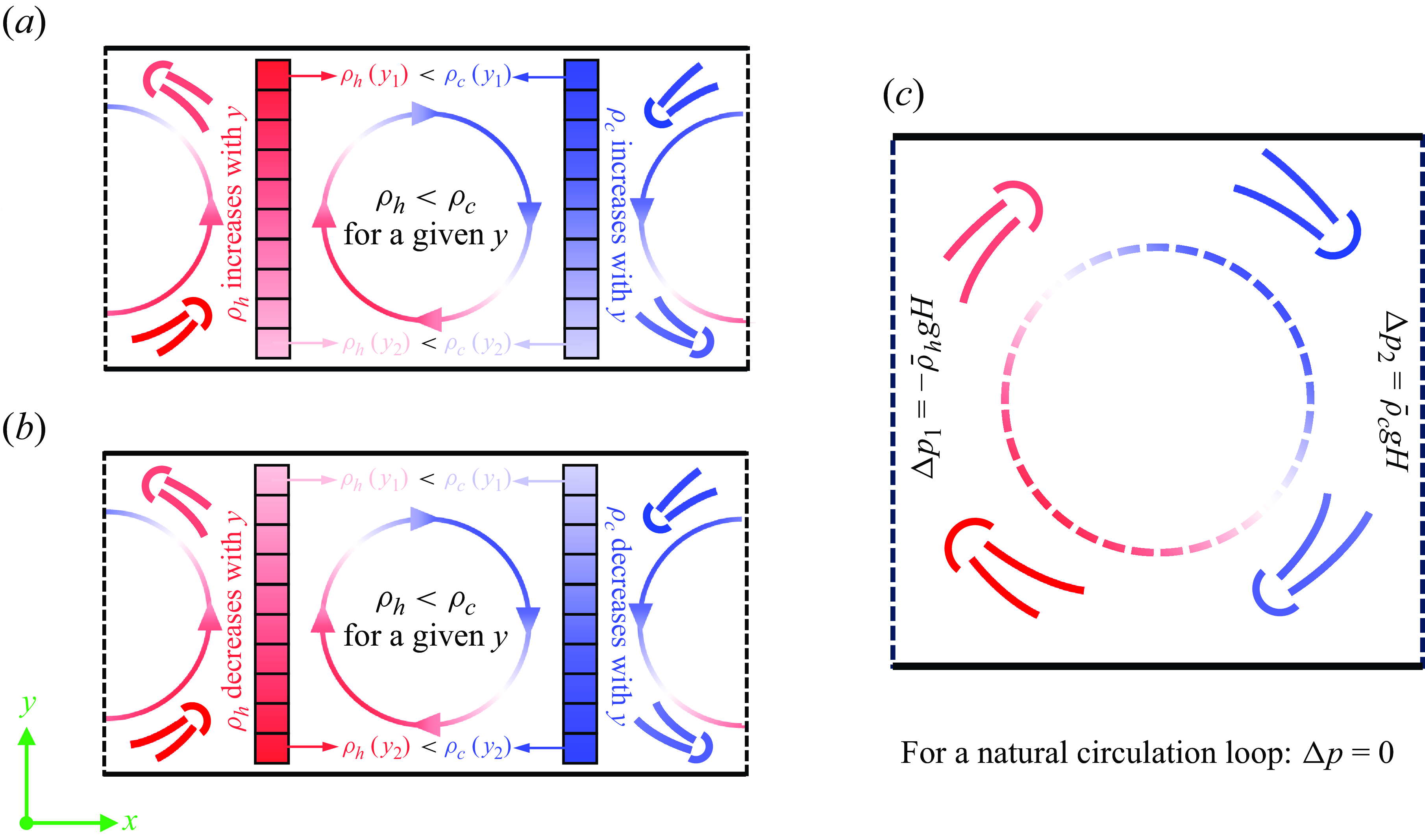
To better explain the flow mechanism when density inversion occurs, we schematically depict the flow structure of RBC in figure 11. As shown in figure 11(a) and 11(b), when density inversion is not present, the densities of both the hot and cold plumes increase as
 $y$
increases. For a given
 $y$
, the density of the hot plume is lower than that of the cold plume. When density inversion occurs, the densities of both the hot and cold plumes decrease as
 $y$
increases. Meanwhile, for a given
 $y$
, the density of the hot plume remains lower than that of the cold plume. We elaborate on the example of one cycle consisting of half a hot plume and half a cold plume, as is illustrated in figure 11(c). It can be seen in figure 10(a) that the flow velocity at the cycle centre is very low. Therefore, we can abstract the cycle as a natural circulation loop (Misale et al. Reference Misale, Garibaldi, Passos and de Bitencourt2007), with the dashed line at the centre of the loop representing the virtual boundary. For the natural circulation loop depicted in figure 10(c), the gravitational pressure drop on the left side is
 $\Delta p_{\mathrm {1}}=-\bar {\rho }_{{h}}gH$
and the gravitational pressure drop on the right side is
 $\Delta p_2=\bar {\rho }_{{c}}gH$
, where
 $\bar {\rho }_{{h}}$
and
 $\bar {\rho }_{{c}}$
represent the average densities of the hot and cold plumes, respectively. In addition, wall friction introduces a frictional pressure drop
 $\Delta p_{\mathrm {3}}=-\Delta p_{ {f}}$
, where
 $\Delta p_{ {f}}$
is positive. The total pressure drops is given by
 $\Delta p= (\bar {\rho }_{{c}}-\bar {\rho }_{ {h}})gH-\Delta p_{ {f}}$
. It is well known that, for a steady-state natural circulation loop, the net pressure drop must be zero. From the above analysis, we observe that
 $\bar {\rho }_{h}$
is lower than
 $\bar {\rho }_{{c}}$
. In this case,
 $\Delta p$
can be equal to 0, allowing the circulation to persist. A similar analysis of the stable stratification in penetrative RBC reveals that, for a given
 $y$
,
 $\bar {\rho }_{ {h}}$
is always greater than
 $\bar {\rho }_{{c}}$
. In this case, the total pressure drop is necessarily negative, and convection cannot persist.
To briefly summarise, under NOB-II conditions, the density of the hot plume is always less than that of the cold plume for a given
 $y$
, regardless of whether density inversion occurs. The buoyancy difference due to the density difference between the two drives the convection to persist. The flow mechanism is very similar to a natural circulation loop.
(a) Schematic of the flow structure and density distribution when the density field is not inverted. (b) Schematic of the flow structure and density distribution when the density field is inverted. (c) Schematic of one cycle consisting of half a hot plume and half a cold plume.
 $\rho _{ {h}}$
represents the density of the hot plume,
 $\rho _{{c}}$
represents the density of the cold plume, and
 $\Delta p_1$
and
 $\Delta p_2$
represent the gravitational pressure drops on the left and right sides of the cycle, respectively.

4.3. Condition for density inversion
Building on our understanding of the convective mechanism, we now seek to identify the conditions under which density inversion occurs. To this end, we define the normalised density difference:
 \begin{align} \Delta \widetilde {\rho } = \widetilde {\rho }_{ {t}}-\widetilde {\rho }_{ {b}} = \frac {\rho _{ {t}}-\rho _{ {b}}}{\rho _{{m}}\beta \Delta T}. \end{align}
where
 $\rho _{{b}}$
and
 $\rho _{{t}}$
represent the mean densities of the bottom and top plates, respectively. Apparently,
 $\Delta \widetilde {\rho }$
is equal to 1 under OB conditions and
 $\Delta \widetilde {\rho } \lt 0$
indicates the occurrence of density inversion. Density is determined by both temperature and pressure. Thus, the density difference
 $\Delta \rho$
arises from the effects of temperature and pressure. The density difference from temperature is given by
 \begin{align} \Delta \rho _T = (T_{ {t}}-T_{ {b}})\left (\frac {\partial \rho }{\partial T}\right )_p = \rho _{{m}}\Delta T \frac {1}{\rho _{{m}}}\left (\frac {\partial \rho }{\partial T}\right )_p = \rho _{{m}}\beta \Delta T. \end{align}
The density difference from pressure can be expressed as
 \begin{align} \Delta \rho _p = (p_{ {t}}-p_{ {b}}) \left (\frac {\partial \rho }{\partial p}\right )_T =\rho _{{m}} gH \left (\frac {\partial \rho }{\partial p}\right )_T. \end{align}
Since the
 $\rho$
,
 $p$
and
 $T$
satisfy equation of state (2.14), triple product rule exists (see Elliott & Lira Reference Elliott and Lira2012, (6.15)):
 \begin{align} \left (\frac {\partial \rho }{\partial p}\right )_T \left (\frac {\partial p}{\partial T}\right )_\rho \left (\frac {\partial T}{\partial \rho }\right )_p = -1. \end{align}
Thus,
 $\Delta \rho _p$
can be further expressed as
 \begin{align} \Delta \rho _p = -\rho _{{m}} gH \left (\frac {\partial \rho }{\partial T}\right )_p \left (\frac {\partial T}{\partial p}\right )_\rho = -\rho ^2_{{m}} gH \beta \left (\frac {\partial T}{\partial p}\right )_\rho. \end{align}
Considering (2.19), the adiabatic temperature difference can be written in the following form (Kogan et al. Reference Kogan, Murphy and Meyer1999; Meyer & Kogan Reference Meyer and Kogan2002):
 \begin{align} \Delta T_{ {ad}} = \frac {gT\beta H}{c_p} = \rho _{{m}} g H\frac {T}{\rho _{{m}}^2 c_p}\left (\frac {\partial \rho }{\partial T}\right )_p \left (\frac {\partial p}{\partial T}\right )_\rho \left (\frac {\partial T}{\partial p}\right )_\rho = \rho _{{m}} g H \frac {c_p-c_v}{c_p}\left (\frac {\partial T}{\partial p}\right )_\rho. \end{align}
Thus,
 $\Delta \rho _p$
can also be expressed as
 \begin{align} \Delta \rho _p = -\frac {c_p}{c_p-c_v}\rho _{{m}}\beta \Delta T_{ {ad}} = -\frac {c_p}{c_p-c_v} \Delta \rho _{ {ad}}, \end{align}
where
 $\Delta \rho _{ {ad}}$
is the density difference from ATG. We assume that the effects of temperature and pressure on the density difference are independent of each other. At this point, the normalised density difference can be expressed as
 \begin{align} \Delta \widetilde {\rho } = \frac {\Delta \rho _T + \Delta \rho _p}{\rho _{{m}}\beta \Delta T} = 1 - \frac {c_p}{c_p - c_v}\alpha. \end{align}
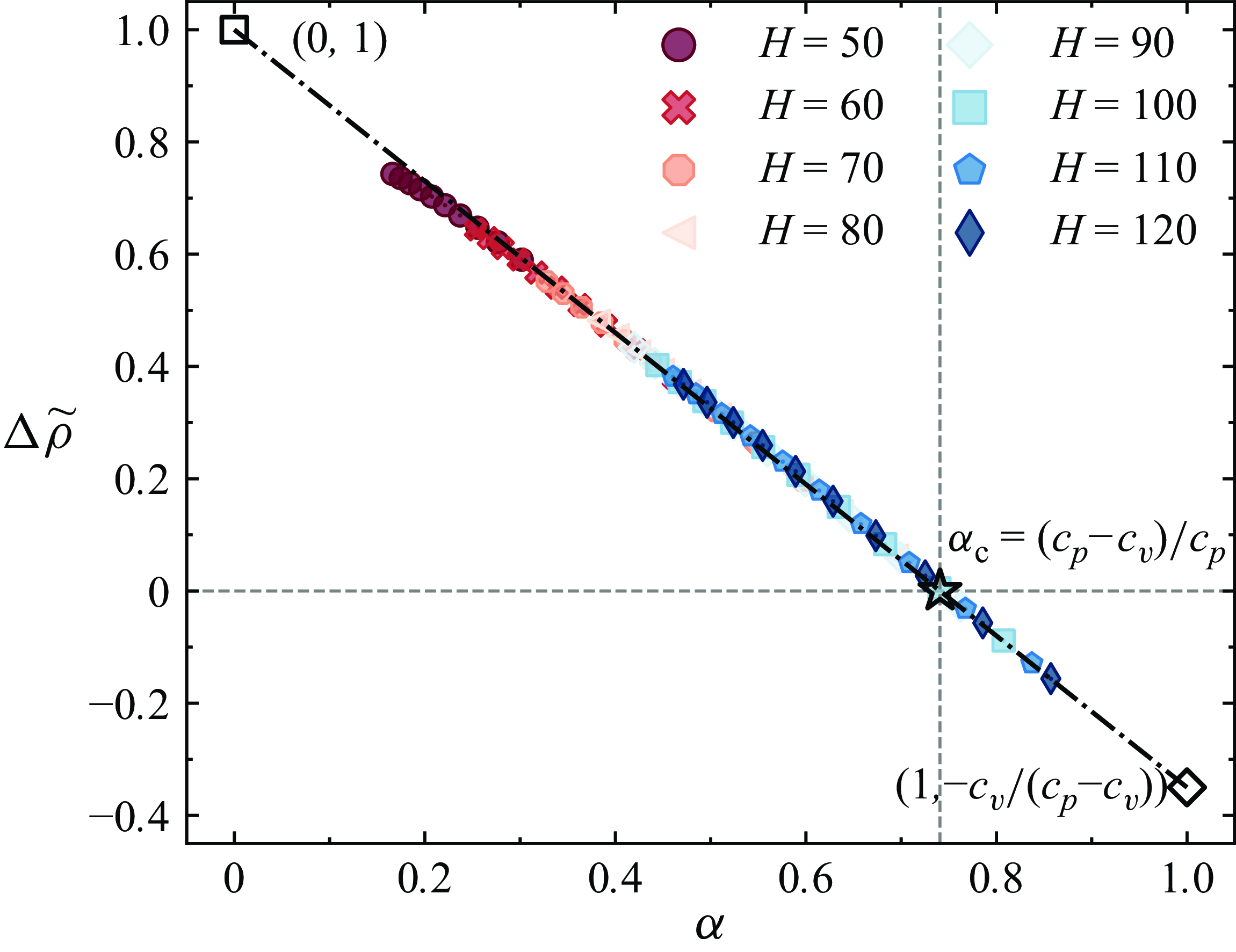
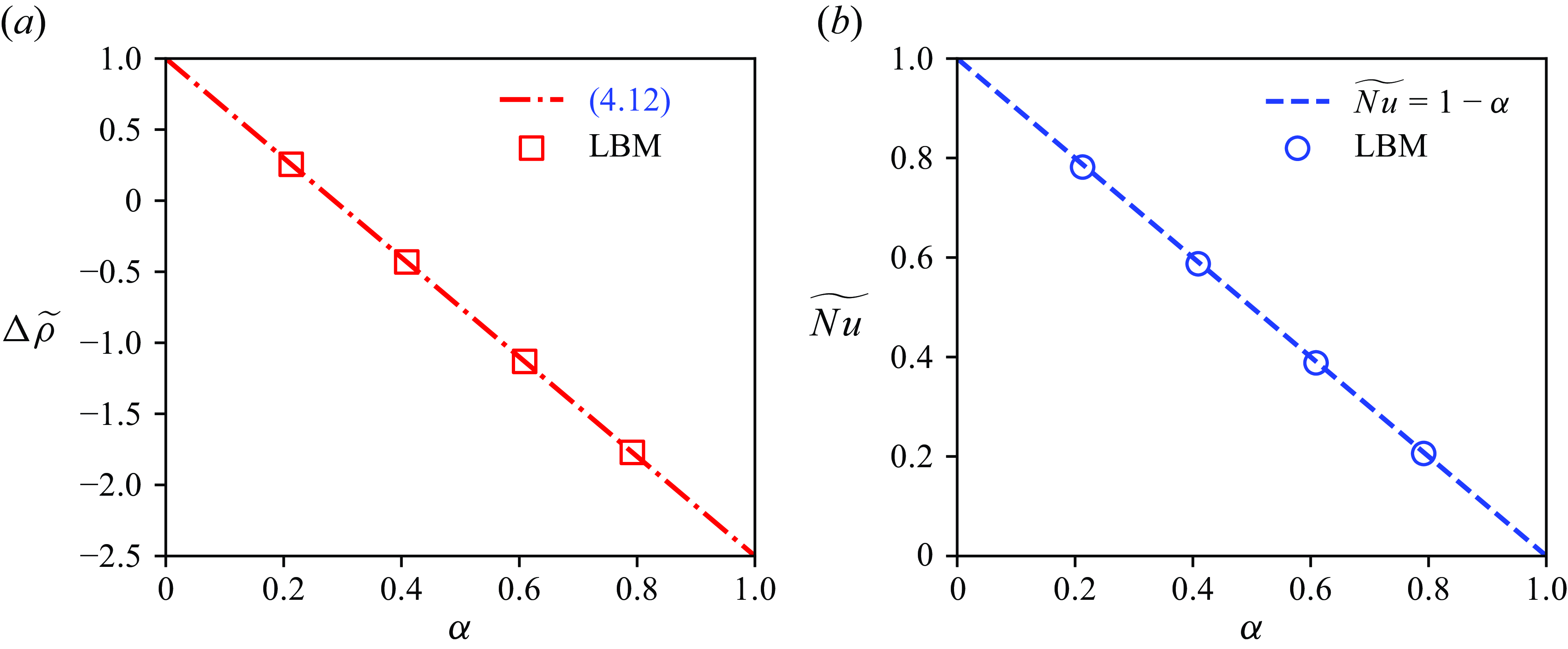
We present both our theoretical results (4.12) and the calculated data in figure 12. Notably, the calculated data closely align with the predictions of (4.12). They both show that the condition for density inversion is
 $\alpha \gt (c_p - c_v)/{c_p}$
. Furthermore, (4.10) indicates that the precondition for density inversion is the inability of the density difference from ATG to fully counterbalance the density difference from pressure. From (4.6) and (4.11), the following equation can also be derived:
 \begin{align} \alpha = \frac {\Delta T_{ {ad}}}{\Delta T_{ {on}}} = \frac {\Delta \rho _{ {ad}}}{\Delta \rho _T} = -\frac {c_p-c_v}{c_p}\frac {\Delta \rho _p}{\Delta \rho _T}. \end{align}
This indicates that
 $\alpha$
is proportional to the ratio of the density difference from pressure to that from temperature. The above analyses suggest that
 $\alpha$
does indicate the intensity of NOB-II effects well.
4.4. Nusselt number
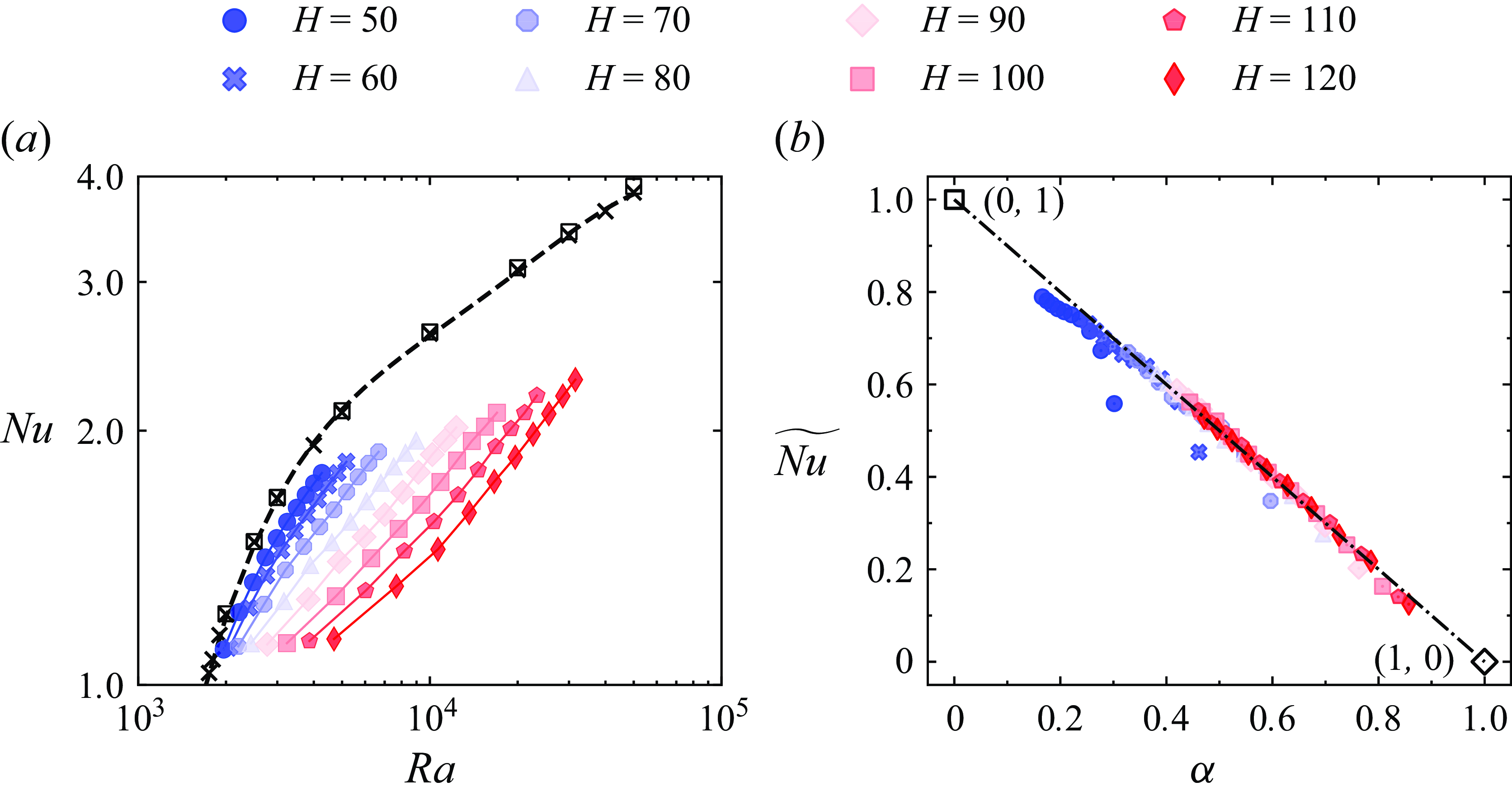
Next, we analyse the impact of NOB-II effects on heat transfer. Figure 13(a) illustrates the variation of the Nusselt number
 $ Nu$
with Rayleigh number
 $ Ra$
. The results clearly show that NOB-II effects deteriorate the heat transfer, as
 $ {Nu}$
is consistently lower than that of OB-RBC for a given
 $ Ra$
. Additionally, for a given
 $ Ra$
, the larger the
 $H$
, the smaller the
 $ Nu$
. We also calculated
 $Nu$
of OB-RBC across various
 $Ra$
using the thermal lattice Boltzmann method presented by Gao et al. (Reference Gao, Yu, Yang, Qin and Hou2021). The results show that the calculated results closely align with the results reported by Clever & Busse (Reference Clever and Busse1974). The slight deviation observed in figure 13(a) arises from the difference in
 $Pr$
. Clever & Busse (Reference Clever and Busse1974)set
 $Pr$
to 7.0, while in our calculations, we used a
 $Pr$
value of 8.25, which corresponds to supercritical fluid at
 $T_{{m}} = 1.05T_{ {cr}}$
and
 $p_{{m}} = 2p_{ {cr}}$
. Previous studies by Clever & Busse (Reference Clever and Busse1974) have already indicated that
 $Nu$
decreases slightly with increasing
 $Pr$
when
 $Pr \gt 2$
.
Variation of the normalised density difference between the top and bottom plates
 $\Delta \widetilde {\rho }$
with
 $\alpha$
for various heights. The dash-dotted line represents the theoretical prediction of (4.12). Ten data points for each
 $H$
represent varying
 $\Delta T$
values, specifically from 1.1 to
 $2.0\Delta T_{ {on}}$
in increments.

(a) Variation of Nusselt number
 $Nu$
with Rayleigh number
 $Ra$
for various
 $H$
. Black square points represent the results of OB-RBC from Clever & Busse (Reference Clever and Busse1974). Black cross points represent the calculated results of OB-RBC using the thermal lattice Boltzmann method presented by Gao et al. (Reference Gao, Yu, Yang, Qin and Hou2021). Dashed line is the best fitting of black cross points. (b) Variation of normalised Nusselt number
 $\widetilde {Nu}$
with
 $\alpha$
for various
 $H$
. Ten data points for each
 $H$
represent varying
 $\Delta T$
values, specifically from 1.1 to
 $2.0\Delta T_{ {on}}$
in increments.

To further quantify the heat transfer deterioration, we define the normalised Nusselt number as follows:
 \begin{align} \widetilde {Nu} = \frac {Nu-1}{Nu_{ {ob}}-1}, \end{align}
where
 $ Nu_{ {ob}}$
is the Nusselt number for the same
 $ Ra$
under OB conditions, obtained by fitting the black cross points in figure 13(a). The variation of
 $ \widetilde {Nu}$
with
 $ \alpha$
for various heights is shown in figure 13(b). The results indicate that the points fall nicely on the line
 $ \widetilde {Nu} = 1 - \alpha$
. This demonstrates that as
 $ \alpha$
increases from 0 to 1,
 $Nu$
decreases linearly from
 $Nu_{ {ob}}$
to 1, indicating significant heat transfer deterioration. Additionally, this further confirms that
 $\alpha$
is a reliable indicator of NOB-II intensity. Notably, several blue outliers are observed in figure 13(b), which primarily arise from the proximity of their
 $Ra$
to
 $Ra_{{c}}$
. This near-critical condition results in
 $Nu_{ {ob}}$
approaching unity, thereby causing the denominator in (4.14) to approach zero and consequently amplifying numerical uncertainties.
4.5. Reynolds number
(a) Variation of Reynolds number
 $Re$
with Rayleigh number
 $Ra$
for various height
 $H$
. (b) Variation of Reynolds number
 $Re$
with reduced Rayleigh number
 $Ra^{\ast}$
for various height
 $H$
. Black asterisk points represent the calculated results of OB-RBC using the thermal lattice Boltzmann method presented by Gao et al. (Reference Gao, Yu, Yang, Qin and Hou2021). The solid line
 $Re=1.042(Ra^*)^{0.541}$
is the best power-law fit to asterisk points. Ten data points for each
 $H$
represent varying
 $\Delta T$
values, specifically from 1.1 to
 $2.0\Delta T_{ {on}}$
in increments.

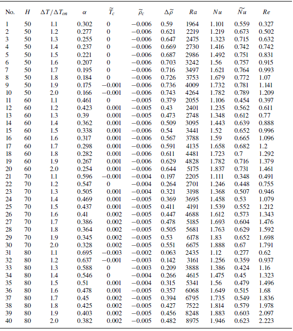
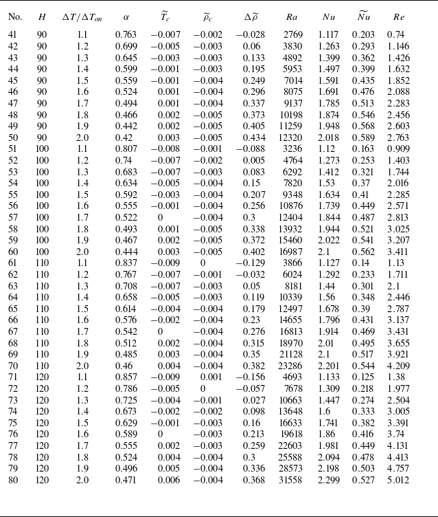
We use the Reynolds number
 $Re$
to indicate the convective intensity and
 $Re$
is defined as follows (Shishkina & Wagner Reference Shishkina and Wagner2016):
 \begin{align} Re = \frac {UH}{\nu }, \quad U = \sqrt {\left \lt \boldsymbol {u\cdot u}\right \gt _{x,y}}, \end{align}
where
 $\left \lt \cdot \right \gt _{x,y}$
denotes the spatial average over the
 $x$
and
 $y$
directions,
 $U$
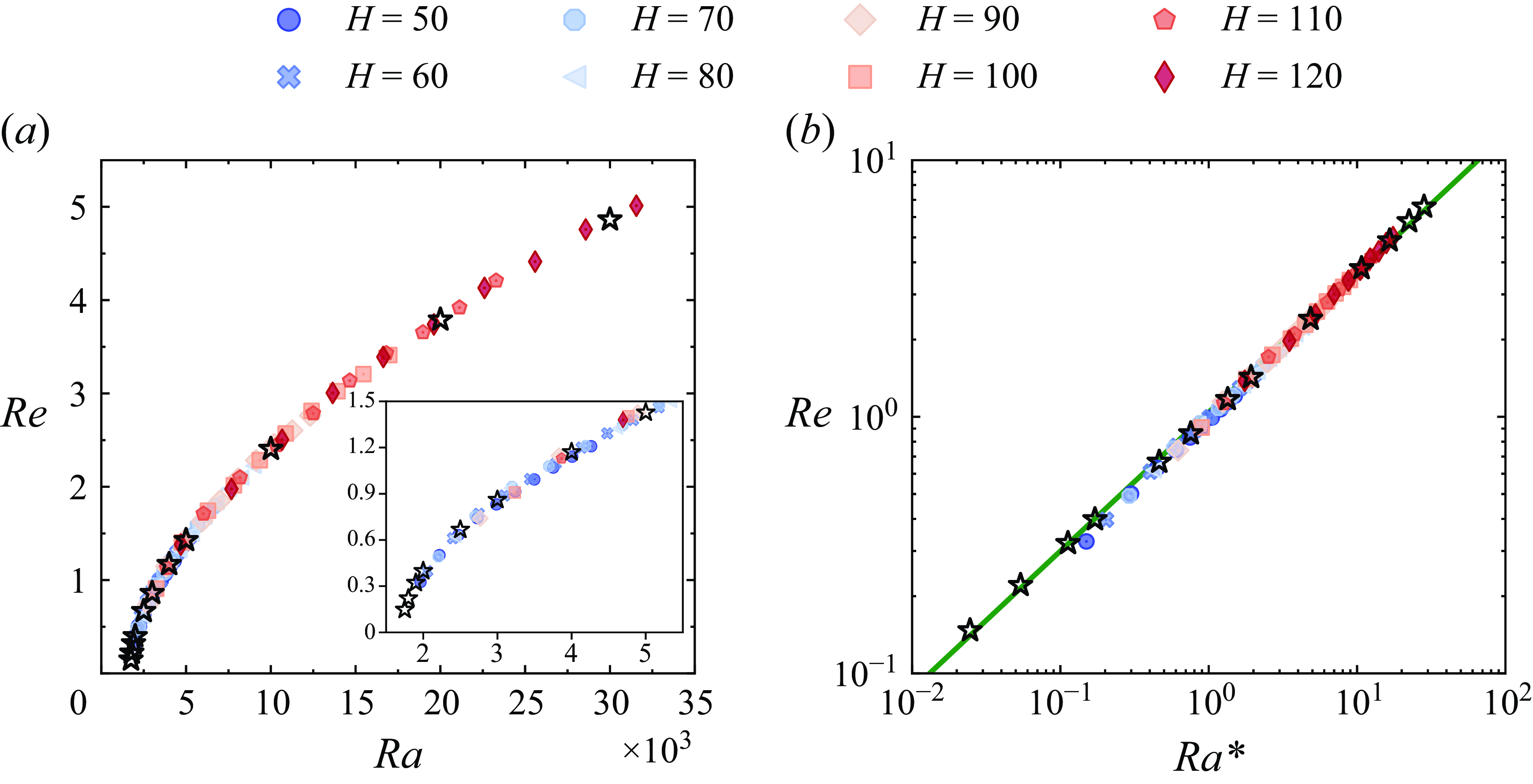
represents the characteristic velocity. Figure 14(a) shows the variation of
 $Re$
with
 $Ra$
for various
 $H$
. The results indicate that
 $Re$
increases with
 $Ra$
. Meanwhile,
 $H$
has no impact on the relation between
 $Re$
and
 $Ra$
, as all points under both OB and NOB-II conditions fall on the same curve. Figure 14(b) shows the variation of
 $Re$
with
 $Ra^*$
. Under OB and NOB-II conditions, all points follow the same power-law relationship
 $Re=1.042 (Ra^* )^{0.541}$
, further confirming the above conclusion.
Combined with the discussion in § 4.4, we observe a unique phenomenon: under dominant NOB-II effects, despite the persistence of vigorous convection, the heat transfer efficiency decreases to a level comparable to pure heat conduction. In other words, as
 $\alpha$
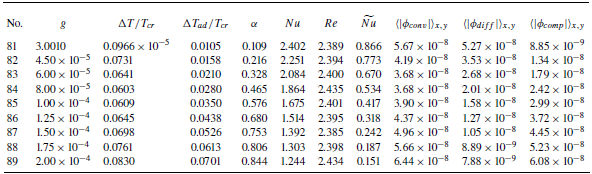
approaches 1, convection ceases to enhance heat transfer relative to pure conduction. The mechanism underlying this significant HTD urgently needs to be explored.
4.6. Mechanism behind heat transfer deterioration
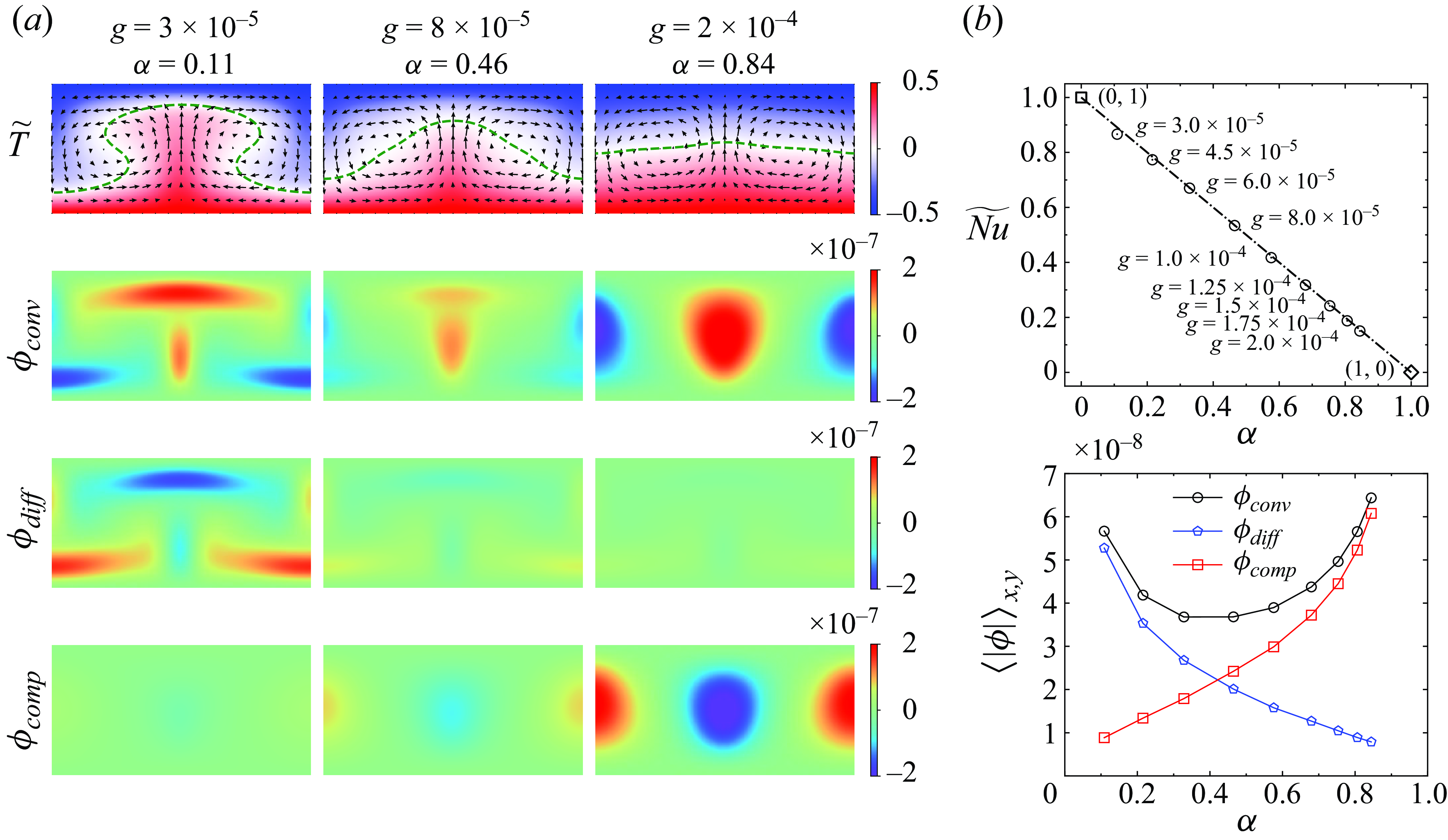
To understand the mechanism behind HTD resulting from NOB-II effects, we first analyse the temperature field. As shown in figure 15(a), as
 $\alpha$
increases, the convective intensity remains essentially unchanged, as reflected by the arrows. However, the temperature distribution becomes progressively flatter as
 $\alpha$
increases. When
 $\alpha = 0.84$
, the temperature distribution closely resembles that of pure heat conduction, characterised by a zero gradient in the
 $x$
-direction and a linear decrease in the
 $y$
-direction. At this point, HTD is observed, as shown in figure 15(b). This suggests that an unknown mechanism is absorbing the heat carried by the hot plume, thereby reducing its ability to transport heat to the top plate. We further investigate this mechanism by examining the energy conservation equation, which is given by
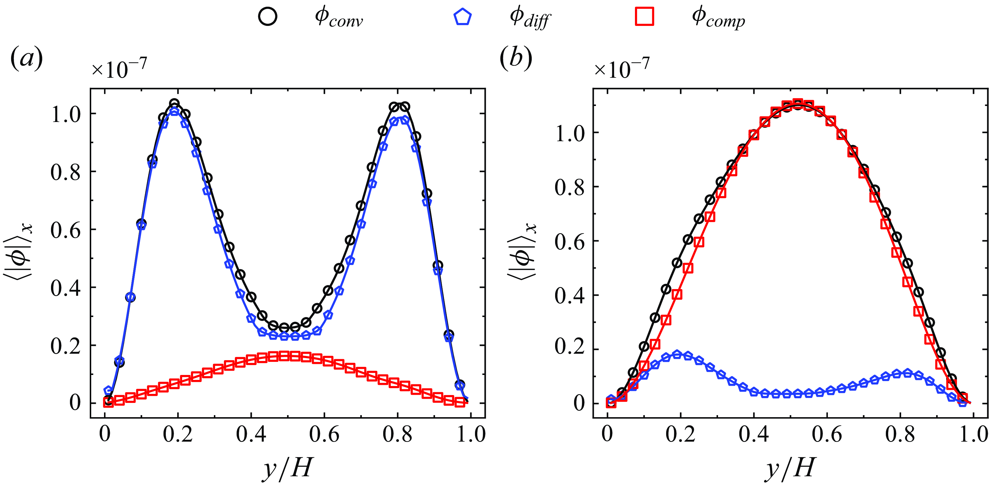
 \begin{align} \frac {\partial T}{\partial t} = \underbrace {-\boldsymbol {u\cdot \nabla } T}_{\displaystyle \phi _{\textit{conv}}} + \underbrace {\frac {1}{\rho c_p}\boldsymbol {\nabla \cdot }(\lambda \boldsymbol {\nabla } T)}_{\displaystyle \phi _{\textit{diff}}} + \underbrace {\frac {1}{\rho c_p}\left (\frac {\partial \mathrm {ln}\rho }{\partial \mathrm {ln}T}\right )_p\frac {\mathrm {d} p}{\mathrm {d} t}} _{\displaystyle \phi _{\textit{comp}}} ,\end{align}
where
 $\mathrm {d} p/\mathrm {d} t = \partial p/\partial t + \boldsymbol {u \cdot \nabla } p$
and (4.16) is equivalent to (2.18) (Moukalled et al. Reference Moukalled, Mangani and Darwish2016). Here, the first term on the right-hand side represents convection term (
 $\phi _{\textit{conv}}$
), the second term represents diffusion term (
 $\phi _{\textit{diff}}$
) and the third term represents compression work term (
 $\phi _{\textit{comp}}$
), which is ignored under OB conditions (Johnston & Doering Reference Johnston and Doering2009).
(a) Normalised temperature
 $\widetilde {T}$
, convection item
 $\phi _{\textit{conv}}$
, diffusion item
 $\phi _{\textit{diff}}$
and compression work item
 $\phi _{\textit{comp}}$
(from top to bottom panel) contours at
 $H=100$
and
 $Ra=10^4$
for various
 $g$
. The green dashed lines represent
 $\widetilde {T}=0$
. (b) Variation of normalised Nusselt number
 $\widetilde {Nu}$
with
 $\alpha$
. The corresponding
 $g$
is indicated in the figure. (c) Variation of the spatial-averaged of the absolute value of source term
 $\langle |\phi |\rangle _{x,y}$
with
 $\alpha$
. Black circle points represent the results of
 $\phi _{\textit{conv}}$
. Blue pentagon points represent the results of
 $\phi _{\textit{diff}}$
. Red square points represent the results of
 $\phi _{\textit{comp}}$
. Connect points with lines for visual enhancement.

Figure 15(c) shows the spatial-averaged of the absolute value of
 $\phi$
,
 $ \left \lt |\phi |\right \gt _{x,y}$
, as a function of
 $ \alpha$
. The results indicate that
 $ \left \lt |\phi _{\textit{diff}}|\right \gt _{x,y}$
decreases with increasing
 $ \alpha$
, while
 $ \left \lt |\phi _{\textit{comp}}|\right \gt _{x,y}$
increases with increasing
 $ \alpha$
. The contours of
 $\phi$
in figure 15(a) reveal that when NOB-II effects are weak, the diffusion and convection terms dominate and the compression term is negligible. This observation is consistent with figures 15(c) and 16(a). Since the diffusion term is related to the temperature gradient, it primarily acts near the plates, where the temperature gradient is the largest (Demou & Grigoriadis Reference Demou and Grigoriadis2019; Wan et al. Reference Wan, Wang, Wang, Xia, Zhou and Sun2020), as shown in figure 8(a). Therefore,
 $\langle |\phi _{\textit{conv}}|\rangle _{x}$
and
 $\langle |\phi _{\textit{diff}}|\rangle _{y}$
present two peaks at the region near the plates, as shown in figure 16(a). At this point, the heat transfer mechanism is that the thermal plume carries the hot fluid near the bottom plate to the top, and then the heat of thermal plume is transfered to the top plate by thermal diffusion. This heat transfer mechanism enables the transfer of heat from the top plate to the bottom plate.
Variation of the horizontal-averaged of the absolute value of source term
 $\langle |\phi |\rangle _{x}$
with
 $y/H$
for (a)
 $g=3\times 10^{-5}$
and (b)
 $g=2\times 10^{-4}$
at
 $H=100$
and
 $Ra=10^4$
. Black circle points represent the results of
 $\phi _{\textit{conv}}$
. Blue pentagon points represent the results of
 $\phi _{\textit{diff}}$
. Red square points represent the results of
 $\phi _{\textit{comp}}$
. Connect points with lines for visual enhancement.

In contrast, when NOB-II effects are strong, the compression and convection terms dominate, while the diffusion term is negligible, as shown in figures 15(a), 15(c) and 16(b). According to (4.16), the compression work term is related to
 $\boldsymbol {u \cdot \nabla } p$
. Although the pressure gradient is uniform throughout the domain (
 $\boldsymbol {\nabla } p \approx \rho \boldsymbol {g}$
), the velocity is higher in the central region and lower near the plates. Additionally, the velocity of the plume in the central region is parallel to the pressure gradient, whereas near the plates, it is perpendicular to the pressure gradient, as shown by the velocity vectors in figure 15(a). As a result, the compression term is larger in the central region and smaller near the plates, as illustrated in figures 15(a) and 16(b). At this point, the heat transfer mechanism changes: when thermal plumes transport hot fluid from the bottom plate to the top plate, the heat of thermal plume is absorbed in the central region by the compression work term. By the time the heat plume reaches the top, its temperature is significantly reduced, greatly reduceing its ability to transfer heat to the top plate. Consequently, the overall heat transfer from the bottom plate to the top plate is significantly impaired.
It is important to clarify that the previous mention of ‘the compressible work term absorbing heat’ is a metaphorical expression. In reality, the flow of fluid along in the opposite direction of the pressure gradient will lead to expansion, and the decrease in temperature during this process is a fundamental characteristic of compressible fluids.
4.7. Perfect gas
The above analysis and discussion pertain to supercritical fluids. However, our analysis is applicable to any compressible fluid. In this section, we perform simulations for a perfect gas to demonstrate the generalisability of our conclusions. The equation of state for a perfect gas is
 $ p = \rho RT$
. To align with the physical properties of air at room temperature, we take the following values for the parameters:
 $ R = 1.6$
,
 $ \nu = 0.05$
,
 $ c_v = 4$
,
 $ \lambda = 1.643$
,
 $ T_{{m}} = 0.15$
and
 $ p_{{m}} = 1$
. With these parameter choices,
 $ c_p/c_v = 1.4$
and
 $ Pr = 0.71$
, which correspond to the typical physical properties of air at room temperature. The height of the computational domain in this section is set to 100. The intensity of NOB-II effects is modulated by adjusting the gravitational acceleration.
Figure 17 illustrates the variation of
 $ \widetilde {Nu}$
and
 $ \Delta \widetilde {\rho }$
with
 $ \alpha$
. The results show that density inversion and HTD also occur in a perfect gas. The simulation results are consistent with the conclusions obtained for supercritical fluids. The density difference
 $ \Delta \widetilde {\rho }$
satisfies (4.12) and
 $ \widetilde {Nu}$
decreases from 1 to 0 with increasing
 $\alpha$
, which fully validates the universality of our conclusions for compressible fluids.
(a) Variation of the normalised density difference
 $ \Delta \widetilde {\rho }$
with
 $ \alpha$
for
 $ Ra = 5000$
. (b) Variation of the normalised Nusselt number
 $ \widetilde {Nu}$
with
 $ \alpha$
for
 $ Ra = 5000$
. The four points in each panel, from left to right, correspond to
 $ g$
:
 $ 2 \times 10^{-4}$
,
 $ 3.2 \times 10^{-4}$
,
 $ 4.8 \times 10^{-4}$
and
 $ 7.5 \times 10^{-4}$
.

5. Outlook and closure
Although previous studies have reported the impact of NOB-I effects on the temperature symmetry and heat transfer, the impact of NOB-II effects on symmetry and heat transfer remains unclear. To address these gaps, we conduct LB simulations of Rayleigh–Bénard convection in supercritical fluids. The specific methodology and conclusions are outlined as follows.
-
(i) Methodology: we present an LB model capable of simulating supercritical fluids. This model uses the D2Q9 discrete velocity model and Peng–Robinson equation of state, which is introduced by considering the intermolecular forces proposed by Shan & Chen (Reference Shan and Chen1993, Reference Shan and Chen1994). The energy equation is solved using finite difference method. The model is validated against static cavity, Schwarzschild criterion and experimental data of Kogan et al. (Reference Kogan, Murphy and Meyer1999). The best power-law fit to the LB results is
 $j/(1-\alpha ) = 1.517 (Ra^*)^{1.116}$
, which is consistent with the experimental data of
$j/(1-\alpha ) = 1.465 (Ra^*)^{1.125}$
. This good agreement demonstrates the potential of LBM for simulating supercritical fluids.
-
(ii) Symmetry of the flow field: the normalised temperature of centre plane is between -0.01 and +0.01 and there is no clear trend with
$\alpha$
. This implies that the unlike NOB-I effects, NOB-II effects do not cause symmetry breaking in temperature. Meanwhile, the normalised density of the centre plane is also between -0.01 and +0.01, indicating that the density field is also symmetric. However, we observe an asymmetry in the velocity. Upon analysis, it is found that the momentum are still symmetric between the upper and lower regions and that the asymmetry in the velocity is due to the difference in density between the upper and lower regions. -
(iii) Density inversion: for the first time, we report that convection can still occur when the bottom fluid is denser than the top fluid, a phenomenon we term density inversion. The underlying mechanism behind density inversion is attributed to the coupling effect of significant pressure gradient and fluid compressibility. In general, the density decreases with temperature and increases with pressure. While the fluid at the bottom is hotter, it is also subjected to higher pressure due to greater depth. Under significant NOB-II effects, the pressure effect dominates, causing the bottom fluid to have a higher density than the top, leading to density inversion. Meanwhile, both theoretical analyses and LB simulations confirm that the normalised density difference
$\Delta \widetilde {\rho }$
and
$\alpha$
satisfy a good linear relationship
$\Delta \widetilde {\rho } = 1 - \alpha c_p /(c_p-c_v)$
, indicating that the condition for density inversion is
$\alpha \gt (c_p - c_v)/{c_p}$
. -
(iv) HTD: we observe that for a given
$Ra$
, NOB-II effects have no impact on
$Re$
. However, the Nusselt number decreases as
$\alpha$
increases. The normalised Nusselt number and
$\alpha$
satisfy a good linear relationship
$\widetilde {Nu} = 1 - \alpha$
. These results indicate that under dominant NOB-II effects, despite the persistence of vigorous convection, the heat transfer efficiency decreases to a level comparable to pure heat conduction, indicating significant HTD. The mechanism behind HTD is attributed to the compression work term in the energy equation, which absorbs heat from the hot plume in the central region, thereby reducing its capacity to transport heat from the bottom plate to the top.


The scope of the current study primarily focuses on laminar convective states. It remains an open question whether these conclusions hold under turbulent convective conditions. In future work, we aim to further optimise the LB model and develop corresponding code for 3-D turbulence simulations. This will enable an in-depth exploration of the impact of NOB-II effects on turbulent thermal 3-D convection.
Acknowledgements.
We thank Chao Sun, Ying He, Ziyang Zhang, Wenxiang Fang and Haodong Yuan for helpful discussions and suggestions on the manuscript.
Funding.
This work was supported by the Nuclear Power Technology Innovation Center of China (Grant No. HDLCXZX-2023-HD-013).
Declaration of interests.
The authors report no conflict of interest.
Appendix A. Equivalence proof
In this appendix, we demonstrate that the definition of the horizontal and vertical axes in figure 6 is equivalent to that of the horizontal and vertical axes in figure 3 of Kogan et al. (Reference Kogan, Murphy and Meyer1999). In the work of Kogan et al. (Reference Kogan, Murphy and Meyer1999), the transverse coordinate is defined as
 \begin{align} Ra_{{corr}}^*=\left (1+\frac {Ra_{ {R}}}{Ra_{{c}}}\alpha \right ) \frac {Ra_{ {R}}-Ra_{ {R,c}}}{Ra_{ {R,c}}} ,\end{align}
where
 $Ra_{ {R}}$
is the Rayleigh number according to Rayleigh criterion, which is defined as
 \begin{align} Ra_{ {R}}=\frac {\rho c_p g \beta H^3\Delta T}{\lambda \nu }. \end{align}
The vertical coordinate is defined as
 \begin{align} j_{{corr}}=\left (1+\frac {Ra_{ {R}}}{Ra_{{c}}}\alpha \right )\frac {Ra_{ {R}}(Nu-1)}{Ra_{ {R,c}}}. \end{align}
According to (3.2) and (A2), when all parameters are the same except
 $\Delta T$
, we can derive
 \begin{align} Ra = Ra_{ {R}}(1-\alpha ) = Ra_{ {R}}\left (1-\frac {\Delta T_{ {ad}}}{\Delta T}\right ) ,\\[-28pt] \nonumber \end{align}
 \begin{align} \frac {Ra_{ {R}}(\Delta T_1)}{Ra_{ {R}}(\Delta T_2)} = \frac {\Delta T_1}{\Delta T_2}, \\[-24pt] \nonumber \end{align}
 \begin{align} \frac {Ra_{ {S}}(\Delta T_1)}{Ra_{ {S}}(\Delta T_2)} = \frac {\Delta T_1-\Delta T_{ {ad}}}{\Delta T_2-\Delta T_{ {ad}}}. \\[3pt] \nonumber \end{align}
Thus, we can derive
 \begin{align} \begin{aligned} Ra_{ {corr}}^{*} & =\left ( 1+\frac {Ra_{ {R}}}{Ra_{{c}}}\alpha \right ) \left ( \frac {Ra_{ {R}}}{Ra_{ {R},{c}}}-1 \right ) \\ & =\left [ 1+\frac {\Delta T}{\Delta T_{{c}}\left ( 1-\Delta T_{ {ad}}/\Delta T_{{c}} \right )}\frac {\Delta T_{ {ad}}}{\Delta T} \right ] \left ( \frac {\Delta T}{\Delta T_{{c}}}-1 \right ) \\ & =\frac {\Delta T_{{c}}}{\Delta T_{{c}}-\Delta T_{ {ad}}}\left ( \frac {\Delta T}{\Delta T_{{c}}}-1 \right ) \\ & =\frac {\Delta T-\Delta T_{{c}}}{\Delta T_{{c}}-\Delta T_{ {ad}}}, \end{aligned} \\[-24pt] \nonumber \end{align}
 \begin{align} Ra^*=\frac {Ra-Ra_{{c}}} {Ra_{{c}}} =\frac {\Delta T-\Delta T_{ {ad}}}{\Delta T_{{c}}-\Delta T_{ {ad}}}-1 =\frac {\Delta T-\Delta T_{{c}}}{\Delta T_{{c}}-\Delta T_{ {ad}}}. \\[3pt] \nonumber \end{align}
Thus,
 $Ra_{{corr}}^{*}$
and
 $Ra^*$
is proven to be equivalent.
 \begin{align} \begin{aligned} j_{ {corr}} & =\left (1+\frac {Ra_{ {R}}}{Ra_{{c}}}\alpha \right )\frac {Ra_{ {R}}(Nu-1)}{Ra_{ {R,c}}} \\ & =\left [ 1+\frac {\Delta T}{\Delta T_{{c}}\left ( 1-\Delta T_{ {ad}}/\Delta T_{{c}} \right )}\frac {\Delta T_{ {ad}}}{\Delta T} \right ] \frac {\Delta T}{\Delta T_{{c}}}(Nu-1) \\ & =\frac {\Delta T_{{c}}}{\Delta T_{{c}}-\Delta T_{ {ad}}}\frac {\Delta T}{\Delta T_{{c}}}(Nu-1) =\frac {\Delta T}{\Delta T_{{c}}-\Delta T_{ {ad}}}(Nu-1), \end{aligned} \end{align}
 \begin{align} \begin{aligned} \frac {j}{1-\alpha } & =\frac {(Nu-1)(Ra^*+1)}{1-\alpha }=(Nu-1)\frac {1}{1-\Delta T_{ {ad}}/\Delta T} \frac {Ra}{Ra_{{c}}} \\ & =(Nu-1)\frac {\Delta T}{\Delta T-\Delta T_{ {ad}}}\frac {\Delta T-\Delta T_{ {ad}}}{\Delta T_{{c}}-\Delta T_{ {ad}}} \\ & =\frac {\Delta T}{\Delta T_{{c}}-\Delta T_{ {ad}}}(Nu-1). \end{aligned} \\[3pt] \nonumber \end{align}
Thus,
 $j_{{corr}}$
and
 $j/(1-\alpha )$
is proven to be equivalent.
Appendix B. Simulation parameters
Simulation parameters are given in tables 2, 3 and 4.
Simulation parameters. The columns from left to right indicate the following: the RBC cell height
 $H$
, the reduced temperature difference
 $\Delta T/\Delta T_{on}$
, the NOB-II parameter
 $\alpha$
, the normalised temperature of the centre plane
 $\widetilde {T}_{{c}}$
, the normalised density of the centre plane
 $\widetilde {\rho }_{{c}}$
, the normalised density difference
 $\Delta \widetilde {\rho }$
, the Rayleigh number
 $Ra$
, the Nusselt number
 $Nu$
, the normalised Nusselt number
 $\widetilde {Nu}$
and the Reynolds number
 $Re$
.

Simulation parameters. The columns from left to right indicate the following: the RBC cell height
 $H$
, the reduced temperature difference
 $\Delta T/\Delta T_{on}$
, the NOB-II parameter
 $\alpha$
, the normalised temperature of the centre plane
 $\widetilde {T}_{{c}}$
, the normalised density of the centre plane
 $\widetilde {\rho }_{{c}}$
, the normalised density difference
 $\Delta \widetilde {\rho }$
, the Rayleigh number
 $Ra$
, the Nusselt number
 $Nu$
, the normalised Nusselt number
 $\widetilde {Nu}$
and the Reynolds number
 $Re$
.

Simulation parameters for
 $Ra=10^4$
. The columns from left to right indicate the following: the gravity
 $g$
, the reduced temperature difference
 $\Delta T/T_{ {cr}}$
, the reduced adiabatic temperature difference
 $\Delta T_{ {ad}}/T_{ {cr}}$
, the NOB-II parameter
 $\alpha$
, the Nusselt number
 $Nu$
, the Reynolds number
 $Re$
, the normalised Nusselt number
 $\widetilde {Nu}$
, the spatial-averaged of the absolute value of convection term
 $\langle |\phi _{ {conv}}|\rangle _{x,y}$
, the spatial-averaged of the absolute value of diffusion term
 $\langle |\phi _{ {diff}}|\rangle _{x,y}$
and the spatial-averaged of the absolute value of compression term
 $\langle |\phi _{ {comp}}|\rangle _{x,y}$
.