1 Introduction
The transport of grains in rivers offers complex interactions among the bed surface, moving grains and water, that has continuously attracted scientists over the last century. Sediment transport on a mobile bed may take place in various conditions. We are focusing on turbulent flows at low Shields values (Shields number represents the dimensionless stress of the flow at the bed) over mild bed-slope. The transport process, under these conditions, is traditionally termed as bed-load and consists of the movement of particles that are entrained from the bed and slide, roll or jump close over it, hitting the particles at rest on the bed surface. After a number of jumps and rebounds, a particle stops in a place where it remains for a ‘resting-time’ interval. A particle movement between two successive periods of repose yields a displacement that Nikora et al. (Reference Nikora, Habersack, Huber and McEwan2002) associated with an intermediate spatial scale. When the Shields value is high enough, a dense sub-layer of moving grains forms in the lower part of the flow (Capart & Fraccarollo Reference Capart and Fraccarollo2011), and the particles rarely stay at rest, sustained by their own collisions (collisionally suspended sediment transport). This can happen also in laminar flows (Ouriemi, Aussillous & Guazzelli Reference Ouriemi, Aussillous and Guazzelli2009). However, the statistics of resting-times and displacements are meaningful only under bed-load conditions. For mono-dispersed bed mixtures, Einstein (Reference Einstein1950) proposed the following law to express
 $q_{s}$
, the volumetric sediment discharge per unit of width
 $$\begin{eqnarray}q_{s}=ELV_{p},\end{eqnarray}$$
based on statistical predictors
 $E$
, the mean number of particles entrained per unit of bed surface and per unit of time, and
 $L$
, the mean travel distance run by particles between two subsequent rests.
 $V_{p}$
is the representative particle volume. Applying (1.1) requires the determination of
 $E$
and
 $L$
as functions of flow and bed conditions. Einstein’s basic conjecture is that
 $L$
is proportional to the grain size, independent of the transport stage, in the bed-load regime. Following Einstein (Reference Einstein1950), several models based on a probabilistic description of the bed-load process have been proposed (Paintal Reference Paintal1971; Nikora et al.
Reference Nikora, Habersack, Huber and McEwan2002; Ancey et al.
Reference Ancey, Böhm, Jodeau and Frey2006; Lajeunesse, Malverti & Charru Reference Lajeunesse, Malverti and Charru2010; Fan et al.
Reference Fan, Zhong, Wu, Foufoula-Georgiou and Guala2014; Fathel, Furbish & Schmeeckle Reference Fathel, Furbish and Schmeeckle2015). Statistical results involving the measurement of local bed-elevation fluctuations in flume experiments suggest that resting-times follow power law distributions associated with long-term sub-diffusive transport while, over longer timescales, they are best described by an exponential distribution (Voepel, Schumer & Hassan Reference Voepel, Schumer and Hassan2013). Travel distances and resting-times are strongly affected by morphological units, such as pools, bars and dunes, which superimpose their transport characteristics (Habersack Reference Habersack2001; Pyrce & Ashmore Reference Pyrce and Ashmore2003; Kasprak et al.
Reference Kasprak, Wheaton, Ashmore, Hensleigh and Peirce2015; Hassan & Bradley Reference Hassan, Bradley, Tsutsumi and Laronne2017). Critical issues to the predictive development proposed by Einstein of (1.1) come from either the proposition of probability distributions without characteristic spatial scales (Ancey et al.
Reference Ancey, Böhm, Jodeau and Frey2006; Ganti et al.
Reference Ganti, Meerschaert, Foufoula-Georgiou, Viparelli and Parker2010; Hill, DellAngelo & Meerschaert Reference Hill, DellAngelo and Meerschaert2010; Campagnol et al.
Reference Campagnol, Radice, Nokes, Bulankina, Lescova and Ballio2013) or from how it deals with particle velocity, resting-time, transition from low to high transport stages, and solid-discharge fluctuation distributions (Ancey et al.
Reference Ancey, Böhm, Jodeau and Frey2006). An important body of research aiming at evaluating entrainment and deposition rates under general flow conditions has recently developed (see Seminara, Solari & Parker Reference Seminara, Solari and Parker2002; Charru, Mouilleron & Eiff Reference Charru, Mouilleron and Eiff2004; Lajeunesse et al.
Reference Lajeunesse, Malverti and Charru2010). This effort permits supplying phenomenological closures for the predictors of (1.1) (or similar) and to make it, eventually, a predictive tool. This work does cover this fundamental issue. To get reliable estimates of the transport predictors in (1.1), the natural approach consists of tracking the trajectories of a large number of grains to obtain information on both step lengths and rest periods (Habersack Reference Habersack2001; Nikora et al.
Reference Nikora, Habersack, Huber and McEwan2002; McNamara & Borden Reference McNamara and Borden2004; Ancey et al.
Reference Ancey, Böhm, Jodeau and Frey2006; Campagnol et al.
Reference Campagnol, Radice, Nokes, Bulankina, Lescova and Ballio2013). Particle-tracking techniques are usually affected by technical limitations and offer, at most, only hundreds of trajectories, which are semi-automatically reconstructed (Campagnol et al.
Reference Campagnol, Radice, Nokes, Bulankina, Lescova and Ballio2013). Seizilles et al. (Reference Seizilles, Lajeunesse, Devauchelle and Bak2014) were able to follow up to approximately 10 000 particle trajectories in a laminar flow, chiefly focusing on lateral transport. Bed-load trajectories referring to poorly sorted sediment-size mixtures and/or to the presence of bed forms, though the expected strong effects of these features on the results, are still not documented in experimental works. To confirm the importance and the need of further experimental analyses on bed-load, a recent paper of Ballio et al. (Reference Ballio, Pokrajac, Radice and Sadabadi2018) bridges Lagrangian and Eulerian outcomes, clarifying limitations of the laboratory set-up with respect to the different reference frames, and enabling operational solutions to be applied.
In contrast with all previous experimental analyses, we provide statistical information on grain movements not based on trajectory reconstruction, but on a straightforward and continuous gauge of the tone of any pixel within a large image sequence. Our procedure is equivalent to obtaining thousands of trajectories and is fully automated, without operator checks and censorship due to the limited sizes of a spatial-temporal observation window (see Ballio et al. Reference Ballio, Radice, Fathel and Furbish2019), allowing us to reach an unprecedented precision in the description of the entrainment process.
Bed-load rate,
 $\tilde{q}_{s}$
and
 $\tilde{t}_{\infty }$
, the dimensionless time needed to reach an almost complete substitution of the pristine particles, for the nine runs.

2 Experimental set-up, run and measurement description
Nine experimental runs were conducted in a 10 cm wide and 6 m long recirculating flume at DICAM, University of Trento, Italy. In each run, sediment and water discharges were constant, and the flow was uniform. Low bed-slopes
 $i_{b}$
were set in all runs (approximately
 $0.3^{\circ }{-}0.5^{\circ }$
). The mobile bed consisted of well-sorted (in size and shape) PVC pseudo-cylindrical grains of equivalent spherical diameter
 $d=3.24\pm 0.08~\text{mm}$
(mean
 $\pm$
standard deviation). The specific submerged density of the particles was
 $\unicode[STIX]{x1D6E5}=\unicode[STIX]{x1D70C}_{s}/\unicode[STIX]{x1D70C}_{w}-1=0.51$
, where
 $\unicode[STIX]{x1D70C}_{s}$
and
 $\unicode[STIX]{x1D70C}_{w}$
are the mass densities of grains and water, respectively. Fall velocity of the particles was approximately
 $w=0.18~\text{m}~\text{s}^{-1}$
and their critical angle of internal friction
 $\unicode[STIX]{x1D6FC}=31^{\circ }$
, measured at very slow shear rates. Most of the grains are white, some are grey, some black. The runs present flow depths
 $h$
between 2–3 cm and flow discharges between
 $5\text{ and }15~\text{l}~\text{m}~\text{s}^{-1}$
. No direct measurements of the flow velocity have been performed.
Variables and results will be reported in dimensionless terms. The dimensionless variables will be denoted by the
 $\tilde{\cdot }$
accent. Our choice is to make times and distances dimensionless by division with, respectively,
 $\sqrt{d/\unicode[STIX]{x0394}g}$
and by
 $d$
, where
 $g$
is the gravitational acceleration. In dimensionless terms, equation (1.1) becomes
 $$\begin{eqnarray}\tilde{q}_{s}=\tilde{E}\tilde{L}\tilde{V}_{p},\quad \text{where }\tilde{q}_{s}=\frac{q_{s}}{\sqrt{g\unicode[STIX]{x0394}d^{3}}},\quad \tilde{E}=E\sqrt{\frac{d^{5}}{g\unicode[STIX]{x1D6E5}}},\quad \tilde{L}=\frac{L}{d},\quad \text{and}\quad \tilde{V}_{p}=\frac{V_{p}}{d^{3}}\approx \frac{1}{2}.\end{eqnarray}$$
Some dimensionless run data are reported in table 1. The recirculated sediment discharge
 $\tilde{q}_{s}$
varied, from run to run, over the range
 $0.014{-}0.200\;(-)$
. The dimensionless value of the sediment discharge, not the Shields stress
 $\tilde{\unicode[STIX]{x1D6E9}}=hi_{b}/(\unicode[STIX]{x0394}d)$
, has been chosen as the reference value to feature the run condition. Though a direct measurement of the Shields stress is available, it is expected to be inaccurate. In fact, it requires measuring the flow depth
 $h$
and the bed-slope
 $i_{b}$
. The flow depth is oscillating a few millimetres in space and time, while the slope is small and its measurement is coarse, affected by errors on even the first digit. On the contrary, the sediment discharge (and the flow discharge, too), measured through volumetric sampling for long time at the outlet of the flume, showed up to be accurate and steady (oscillation within a few
 $\%$
units). To complete the presentation of the hydraulic parameters, calling
 $U$
the average flow velocity and
 $\unicode[STIX]{x1D708}$
the water kinematic viscosity, we report that the Froude number (
 $Fr=U/\sqrt{gh}$
) in the various runs varied approximately between
 $0.4\text{ and }0.6\;(-)$
, the Reynolds number (
 $Re=Uh/\unicode[STIX]{x1D708}$
) approximately between
 $3\times 10^{3}\text{ and }13\times 10^{3}\;(-)$
and the particle Reynolds number (
 $Re_{p}=\sqrt{g\unicode[STIX]{x0394}d}/\unicode[STIX]{x1D708}$
) was approximately
 $400\;(-)$
.
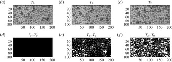
(a–c) Time sequence of three real images, taken at the times
 $T_{i}$
,
 $i=0,1,2$
increasing with the subscript. (d–f) Images obtained after subtracting the first image, taken at
 $T_{0}$
, from the real images of the top row. Units along both axes are dimensionless distances (
 $x$
and
 $y$
divided by
 $d$
).

A video camera positioned approximately 1 m above the free surface was used to record images of the bed surface during the run. Each image covers a bed surface area (BSA) of approximately
 $9\times 35~\text{cm}^{2}$
, consisting of roughly
 $3{-}4\times 10^{3}$
visible grains. Lighting is an important issue. We used two sources of diffused, not flickering, LED lights, which illuminated the bed surface through the transparent sidewall. The lighting is free from outside biases, as the entire flume was covered by a single piece of thick cloth. The recorded images are frames measuring
 $1024~\text{pixel}\times 256~\text{pixel}$
, acquired as matrices having the numbers of rows and columns equal to the sizes, in pixel units, of the image. Figure 1(a–c) shows a portion of the acquired images at three subsequent instants
 $T_{0}$
,
 $T_{1}$
,
 $T_{2}$
. The resolution of the images is high enough to allow us to see and identify the particles lying on the bed surface. A single particle occupies up to 100 pixels. Figure 1(d–f) shows a sequence of special images obtained after subtracting the
 $T_{0}$
image from the real images (see (2.3)). This technique has already been used for other purposes (Heays, Friedrich & Melville Reference Heays, Friedrich and Melville2014) and is termed ‘digital erosion’. The subtraction allows us to assess whether or not any pixel in the current image is occupied by the same grain or group of grains already present in the first image. The particles viewed in the BSA in the first image, at
 $T_{0}$
, are important in our analysis, and will be referred to as ‘pristine’. They form the statistical sample of the present analysis.
We worked through the recorded images of the BSA (figure 1
a–c). Herein, the underscript
 $\infty$
refers to values of quantities at a time equal to, or later than,
 $\tilde{t}_{\infty }$
, (see table 1), a finite time value after which the asymptotic entrainment of all the pristine particles has ended. First, we calculated the dimensionless chromatic area,
 $\tilde{a}(\tilde{t})$
, defined as
 $$\begin{eqnarray}\tilde{a}(\tilde{t})=\frac{a(\tilde{t})}{a_{\infty }},\end{eqnarray}$$
where
 $a(\tilde{t})$
and
 $a_{\infty }$
are
 $$\begin{eqnarray}a(\tilde{t})=\mathop{\sum }_{i=1}^{N}\mathop{\sum }_{j=1}^{M}|\unicode[STIX]{x1D608}_{ij}(\tilde{t})-\unicode[STIX]{x1D608}_{ij}(0)|;\quad a_{\infty }=a(\tilde{t}_{\infty }),\end{eqnarray}$$
with
 $N$
and
 $M$
being the dimensions of the frame matrix; subscripts
 $i,j$
represent the pixel position in the image-frame (i.e., a matrix)
 $\unicode[STIX]{x1D63C}$
. The matrix entries
 $\unicode[STIX]{x1D608}_{ij}$
represent the grade in the grey-scale range (integer values from 0 to 255) of the pixel at position
 $i,j$
of the real image-frame taken at time
 $t$
. The acquired images are standard ‘bmp’ files. To convert them into a matrix, we used MATLAB (‘imread’ function). At
 $\tilde{t}=0$
, the first image (the pristine one) is taken,
 $\unicode[STIX]{x1D608}_{ij}(\tilde{t})$
are the pixel tones of an image-frame taken at the current time
 $\tilde{t}$
;
 $\unicode[STIX]{x1D608}_{ij}(\tilde{t}_{\infty })$
are the pixel tones of an image-frame taken at a later time (
 $\tilde{t}\geqslant \tilde{t}_{\infty }$
), being the asymptotic times
 $\tilde{t}_{\infty }$
reported in table 1.
Any entrainment or deposition of a grain yields variations of the grey-scale grade in the image pixels occupied by that grain (approximately 100 pixels on average per fully visible grain). Entrainment of non-pristine particles lying over non-pristine particles, or deposition of an incoming particle over non-pristine parts of the BSA, provokes local changes of the pixel tones, but no changes on the global function
 $\tilde{a}(\tilde{t})$
. Only the entrainment of pristine particles provokes a steady change of
 $\tilde{a}(\tilde{t})$
. Burial and reappearance of a pristine particle has also substantial effects on
 $\tilde{a}(\tilde{t})$
, but they cancel out as time passes. As time increases after the start of the run, the subtracted images (figure 1
d–f) change from being all black (
 $\text{grey level}=0$
) to becoming images with pixel tones in the whole grey range 0–255 (like any original image in the top row of the figure). The function
 $a(\tilde{t})$
(2.3), tells us how many pristine particles, over their total number, are not visible at time
 $\tilde{t}$
, and is changing from
 $0$
toward its horizontal asymptote. Then, from (2.2),
 $\tilde{a}(\tilde{t})$
is a function starting from 0, at
 $\tilde{t}=0$
, and moving around
 $\tilde{a}=1$
, at
 $\tilde{t}\geqslant \tilde{t}_{\infty }$
. The increase of
 $\tilde{a}$
, from 0 to 1 is not necessarily strictly monotonic. After
 $\tilde{t}_{\infty }$
the pristine bed surface has been almost completely rearranged, i.e., no more pristine particles are still in the place they were at
 $\tilde{t}=0$
. Such a condition is supported by visual inspections of the images and by the function
 $\tilde{a}(\tilde{t})$
asymptotically tending to unity.
The moving particles that appear in the first image are not pristine and move away soon, causing an abrupt increase of the modified area function at the start of the process. This discontinuous jump of
 $a(t)$
, which is smaller in the runs with lower sediment discharge, must be subtracted from the
 $a(t)$
values, so that the modified area function starts from zero. Other temporary changes are due to moving grains passing over the BSA, without stopping on it, or to free-surface wrinkling; these processes alter some spots, but only momentarily, producing meaningless small and quite short fluctuations in the output. These are filtered out by fitting the measured modified areas with analytic functions.
Values of
 $\tilde{a}(\tilde{t})$
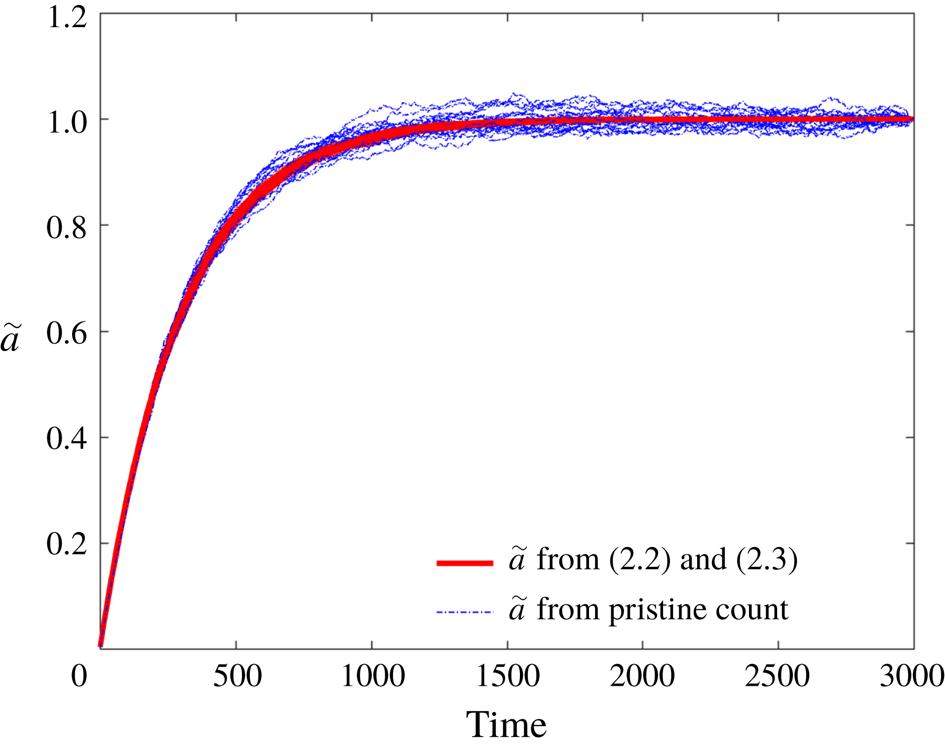
of an artificial image made of
 $N_{t}=3000$
pixels (approximately the number of particles we have in a real image), evolved by randomly substituting, at any time unit, the colour tone of 100 pixels. We calculated
 $\tilde{a}(\tilde{t})$
either by using (2.2)–(2.3) or by counting the number of pristine pixels
 $N_{p}$
at any time and used it as the input in the following expression
 $\tilde{a}(\tilde{t})=1-N_{p}(\tilde{t})/N_{t}$
. We report 20 realisations of the stochastic process.

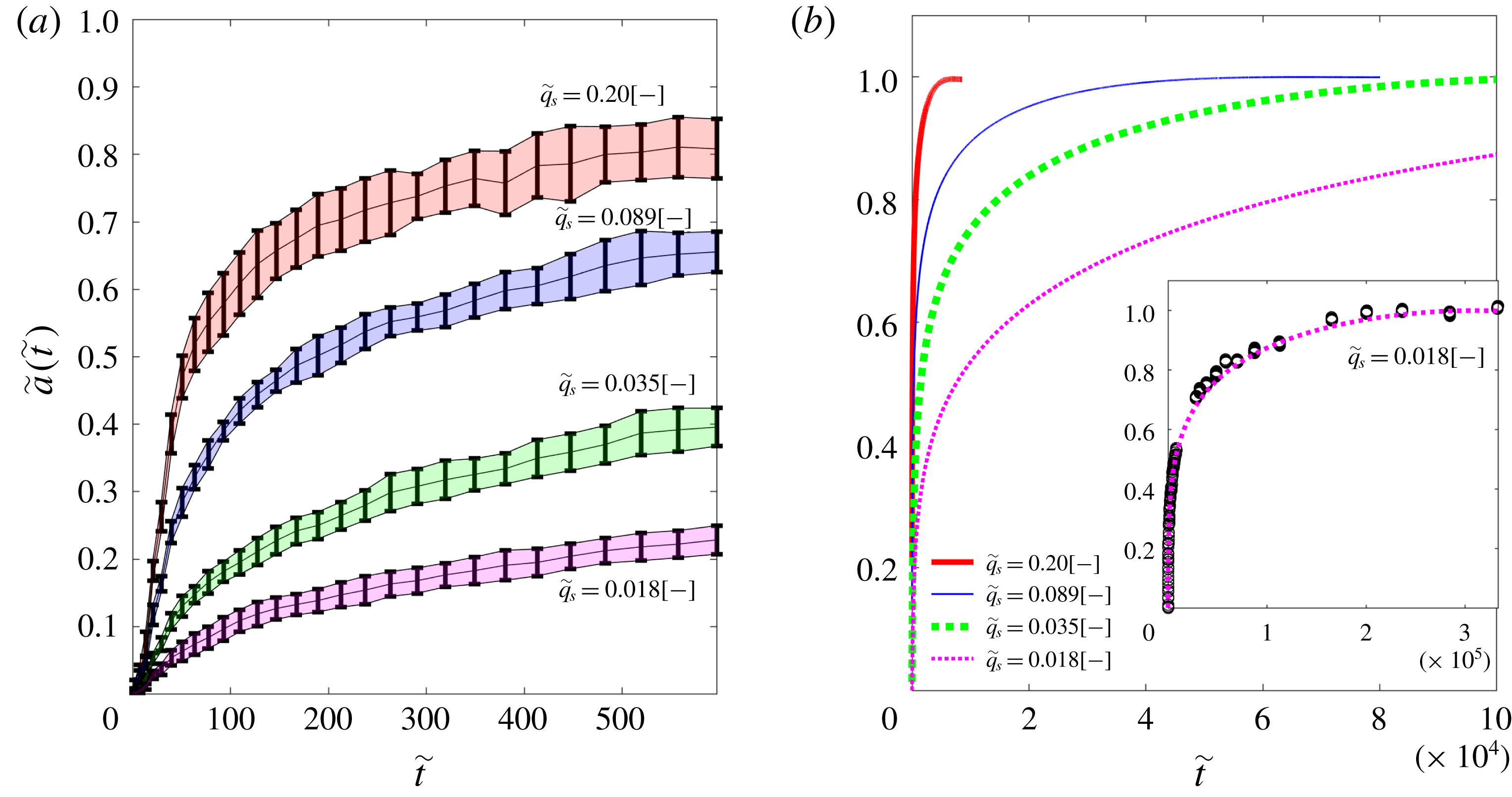
(a) Experimental evolution of
 $\tilde{a}(\tilde{t})$
for four experimental runs, tagged with the relevant values of
 $\tilde{q}_{s}$
The solid lines connect the mean values obtained from several repetitions, the shaded areas envelop the interval bars. (b) Curves representing the analytic fitting of
 $\tilde{a}(\tilde{t})$
, for the same runs of (a), for a longer time interval. The curves stop when the asymptote
 $\tilde{a}(\tilde{t})=1$
is reached. In the inset the fitting curve along with the experimental data (circles) for a single realisation of run
 $\tilde{q}_{s}=0.018\;(-)$
.

A key assumption we make is that the way
 $\tilde{a}(\tilde{t})$
evolves, from 0 to the asymptote 1, represents the percentage of the pristine particles that are either presently covered (at time
 $\tilde{t}$
) or that have been already entrained (before time
 $\tilde{t}$
). Since we are measuring colour tones and do not directly count the pristine particles, the assumption needed to be validated. It has been easily and fully satisfactorily checked by using a stochastic model. Figure 2 shows some relevant results.
In figure 3(a), we present the evolution of the chromatic area
 $\tilde{a}(\tilde{t})$
for four runs. The time window is limited to a few hundred dimensionless time units, thus it may not be evident that all the curves actually tend toward unity. The lower the value of
 $\tilde{q}_{s}$
, the higher the value of
 $\tilde{t}_{\infty }$
(table 1). We repeated most of the runs a few times in order to get a mean value and an interval bar at any time of their evolution. For the same runs and longer times, figure 3(b) shows the analytic functions fitting the
 $\tilde{a}(\tilde{t})$
measurements, with an inset devoted to the slowest run, where all the measurements for a single realisation and the fitting curve are displayed together.
3 Theoretical analysis
Any particle lying on the bed surface is endowed with a stochastic property, the resting-time
 $\tilde{T}_{r}$
, i.e., the time interval (a positive quantity) from its last arrest to its next entrainment. Despite their similarity in all aspects (shape, size, density, etc.), the grains on the bed surface have a different probability of being entrained, reflecting different responses to near-bed fluid turbulence. Different values of
 $\tilde{T}_{r}$
mirror different stability of the grains due to local (at the grain scale) packing, imbrication or flow conditions. Once a particle is entrained, it loses any link to its former condition; when it stops on the bed again, it gains a new value of
 $\tilde{T}_{r}$
, and so on. We assumed that the resting-times associated with the grains on the BSA form a statistical population. Hereafter we describe the theoretical approach that exploits the measured chromatic area
 $\tilde{a}(\tilde{t})$
to get, or approximate, the probability density function
 $p(\tilde{T}_{r})$
of the resting-times. The statistical mean of its inverse,
 $\langle \tilde{T}_{r}^{-1}\rangle$
, is the mean entrainment frequency of the grains on the bed surface. According to the definition of
 $\tilde{E}$
, in (2.1),
 $\langle \tilde{T}_{r}^{-1}\rangle$
is equal to the product of
 $\tilde{E}$
and a particle shape coefficient, that represents the average bed-surface area occupied by a single particle, divided by
 $d^{2}$
and by the volumetric sediment-concentration of the static bed. This coefficient is close to 1 for both closely packed spheres or for uniformly-oriented and aligned cubes, hence it is assumed
 $$\begin{eqnarray}\langle \tilde{T}_{r}^{-1}\rangle \approx \tilde{E}.\end{eqnarray}$$
The start of the recording, when the first image is taken, is chosen to be
 $\tilde{t}=0$
, where
 $\tilde{t}$
is the current time of the evolution process. In a single run, the evolution of the chromatic area
 $\tilde{a}(\tilde{t})$
is modelled through the following equation
 $$\begin{eqnarray}\frac{\text{d}\tilde{a}}{\text{d}\tilde{t}}(\tilde{t})=\underbrace{p_{c}(\tilde{t})}_{\mathit{Pr. Entr. Act}}+\underbrace{\langle \tilde{T}_{r}^{-1}\rangle (1-\tilde{a})}_{\mathit{Pr.Bur.Act}}-\underbrace{\langle \tilde{T}_{r}^{-1}\rangle \int _{0}^{\tilde{t}}(1-\tilde{a}(\unicode[STIX]{x1D709}))p(\tilde{t}-\unicode[STIX]{x1D709})\,\text{d}\unicode[STIX]{x1D709}}_{\mathit{Pr.Reap.Act}},\end{eqnarray}$$
where
 $p_{c}$
is the probability density function (p.d.f.) of the censored resting-times
 $\tilde{T}_{c}$
, i.e, the resting-time interval of the pristine particles calculated from time
 $\tilde{t}=0$
and not from the actual inlet time
 $\tilde{t}_{i}\leqslant 0$
, at which the pristine particle reached its position in the BSA. Because the pristine particles have already been sitting for some time in the position that they occupy at
 $\tilde{t}=0$
,
 $\tilde{T}_{r}=\tilde{T}_{c}-\tilde{t}_{i}\geqslant \tilde{T}_{c}\geqslant 0$
holds. Here
 $\unicode[STIX]{x1D709}$
is a dummy variable for time in the convolution term.
Equation (3.2) is a kind of conservation equation for the exposed surface of the pristine particles that governs the modification of the pixel values of the BSA. Under uniform and steady flow conditions and a flat bed, entrainment and deposition even out at any time, and both contribute to modify the chromatic area. Specifically, three acts affect, during the run, the value of
 $\tilde{a}(\tilde{t})$
. First, when a pristine particle is entrained, a random change occurs in the grey-tone of the pixels occupied by that particle. This is referred to as ‘pristine entrainment act’. Second, a particle coming from upstream can arrive and settle in a position over the BSA. If such a particle covers in part or totally pristine particles, then a temporary change of the grey-tone of the corresponding local pixels takes place. This is referred to as ‘pristine burial act’. Third, when this particle will be later entrained, after even a long residence period, the image of the local pristine bed will be restored. This act will be referred to as ‘pristine reappearance act’. These three acts are mathematically represented in the three terms in the right-hand side of (3.2) and are responsible of the monotonic increment of
 $\tilde{a}(\tilde{t})$
from 0 to 1. The ‘pristine entrainment act’ and the ‘pristine burial act’ terms are always positive and are summed; the last term refers to the ‘pristine reappearance act’ and is positive, but is subtracted. The ‘pristine burial act’ term is proportional to
 $(1-\tilde{a})$
because we assumed that the conditional probability for an arriving particle to stop in the BSA over a pristine (or non-pristine) particle is only equal to the fraction of bed occupied by pristine (or non-pristine) particles. Last contribution (‘pristine reappearance act’) is a convolution integral that involves the distribution
 $p(\tilde{T}_{r})$
. Here we assumed that the probability density function of the resting-times of the arriving, non-pristine, particles, once they deposit, is identical to the
 $p(\tilde{T}_{r})$
of the pristine particles occupying the bed at
 $\tilde{t}=0$
. This term starts from zero, at
 $\tilde{t}=0$
, and ends at zero, at
 $\tilde{t}\geqslant \tilde{t}_{\infty }$
, when no pristine particles may be found and hidden anymore. The integral over time, from 0 to
 $\infty$
, of the difference between the ‘pristine burial act’ term and the ‘pristine reappearance act’ term is null, as can be easily proved by using the Fubini theorem. Hence, from (3.2),
 $\int _{0}^{\infty }p_{c}\,\text{d}\unicode[STIX]{x1D709}=\tilde{a}(\infty )-\tilde{a}(0)=1$
, as expected for a probability density function.
Another relation between
 $p(\tilde{T}_{r})$
and
 $p_{c}(\tilde{T}_{c})$
can be established by considering that the inlet time,
 $\tilde{t}_{i}$
, is also a stochastic variable, fully uncorrelated to
 $\tilde{T}_{r}$
. A pristine particle has an equally distributed probability to have entered the BSA in the time interval
 $[-\tilde{T}_{r},0]$
, with
 $\tilde{T}_{r}$
being its resting-time. Hence, the contribution to
 $p_{c}(\tilde{T}_{c})$
from pristine particles having resting-time
 $\tilde{T}_{r}$
, is proportional to
 $p(\tilde{T}_{r})$
itself, and inversely proportional to
 $\tilde{T}_{r}$
. Keeping in mind that, at any
 $\tilde{t}\geqslant 0$
, only pristine particles having
 $\tilde{T}_{r}\geqslant \tilde{t}$
are still sitting in the BSA, the censored-time p.d.f.,
 $p_{c}(\tilde{T}_{c})$
, is built over just a part of the resting-time p.d.f.,
 $p(\tilde{T}_{r})$
, that is over
 $p(\tilde{T}_{r}\geqslant \tilde{T}_{c})$
. Therefore, stringing all these concepts together, the following expression holds
 $$\begin{eqnarray}p_{c}(\tilde{T}_{c})=\int _{\tilde{T}_{c}}^{\infty }\frac{p(\unicode[STIX]{x1D709})}{\unicode[STIX]{x1D709}}\,\text{d}\unicode[STIX]{x1D709},\end{eqnarray}$$
where
 $\unicode[STIX]{x1D709}$
is a dummy variable for resting-time. Through the Fubini theorem again, it is straightforward to check that
 $\int _{0}^{\infty }p\,\text{d}\unicode[STIX]{x1D709}=1$
, as it must be for a probability density function. From taking the derivative with respect to
 $\tilde{T}_{c}$
of both sides of (3.3), the result is
 $$\begin{eqnarray}p(\tilde{T}_{r})=-\tilde{T}_{c}\frac{\text{d}p_{c}(\tilde{T}_{c})}{\text{d}\tilde{T}_{c}},\quad \text{at }\tilde{T}_{c}=\tilde{T}_{r}.\end{eqnarray}$$
Equations (3.2) and (3.4) form a coupled system in the unknown probability density functions, that is
 $p(\tilde{T}_{r})$
and
 $p_{c}(\tilde{T}_{c})$
. Of course, as the motion is steady uniform, the solutions do not depend on the starting time
 $\tilde{t}=0$
, nor on the choice of the BSA location. In solving (3.2) and (3.4), we replaced the measured chromatic area
 $\tilde{a}(\tilde{t})$
with its fitted analytic function. Its time derivative was then used in (3.2) within the range
 $0\leqslant \tilde{a}\leqslant 0.99$
.
We can further show that
 $p_{c}(0)$
is equal to
 $\langle \tilde{T}_{r}^{-1}\rangle$
, and, in turn, equal to
 $\tilde{E}$
(3.1). To show this, let us build the p.d.f. of the variable
 $\langle \tilde{T}_{r}^{-1}\rangle$
: it, being the inverse of the resting-time, has a p.d.f. equal to
 $p(\tilde{T}_{r})\tilde{T}_{r}^{2}$
; by definition, its mean is
 $$\begin{eqnarray}\langle \tilde{T}_{r}^{-1}\rangle =\int _{\infty }^{0}[p(\unicode[STIX]{x1D709})\unicode[STIX]{x1D709}^{2}]\frac{1}{\unicode[STIX]{x1D709}}\,\text{d}\left(\frac{1}{\unicode[STIX]{x1D709}}\right)=\int _{0}^{\infty }\frac{p(\unicode[STIX]{x1D709})}{\unicode[STIX]{x1D709}}\,\text{d}\unicode[STIX]{x1D709}.\end{eqnarray}$$
Then, from (3.3)
 $$\begin{eqnarray}\int _{0}^{\infty }\frac{p(\unicode[STIX]{x1D709})}{\unicode[STIX]{x1D709}}\,\text{d}\unicode[STIX]{x1D709}=p_{c}(0).\end{eqnarray}$$
This information is important, as it represents a constraint, which must be satisfied in solving the system of (3.2) and (3.4).
More important, from (3.2), evaluated at
 $\tilde{t}=0$
, (3.5) and (3.6) it can be inferred that
 $\langle \tilde{T}_{r}^{-1}\rangle$
is readily available (and so is predictor
 $\tilde{E}$
through (3.1)) from the derivative of
 $\tilde{a}(\tilde{t})$
at
 $\tilde{t}=0$
 $$\begin{eqnarray}\langle \tilde{T}_{r}^{-1}\rangle =p_{c}(0)=\frac{1}{2}\frac{\text{d}\tilde{a}}{\text{d}\tilde{t}}(\tilde{t}=0).\end{eqnarray}$$
4 Results
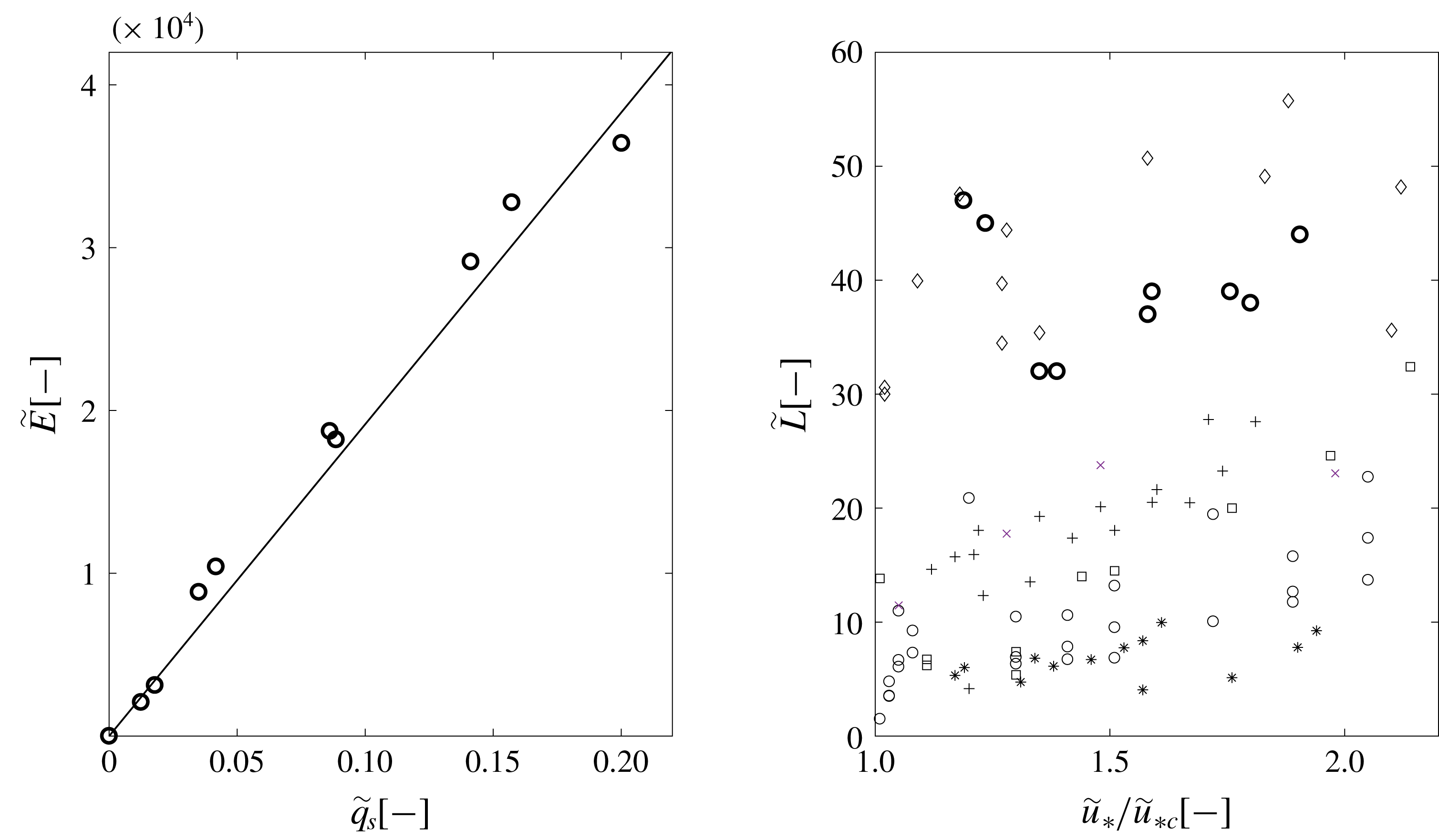
(a) Linear fitting between
 $\tilde{E}$
and
 $\tilde{q}_{s}$
; bold circles represent the measurements. (b) Values of
 $\tilde{L}$
from our measurement (bold circles) and from other authors (from figure 5 of Campagnol, Radice & Ballio (Reference Campagnol, Radice, Ballio, Fry and Chevalier2012)), versus the ratio between friction velocity and its critical value.

From the evolution of the chromatic area, we may directly extract both the predictors
 $\tilde{E}$
and
 $\tilde{L}$
of the sediment discharge relation (2.1). The term
 $\tilde{E}$
comes from (3.7). Figure 4(a) reports the obtained values of
 $\tilde{E}$
versus
 $\tilde{q}_{s}$
; they appear to vary in a proportional way. Their relation is fitted with the line defined in following equation (4.1), crossing the origin and having a
 $R^{2}$
regression coefficient equal to approximately 0.98
 $$\begin{eqnarray}\tilde{E}=\unicode[STIX]{x1D6FD}\tilde{q}_{s},\quad \text{with }\unicode[STIX]{x1D6FD}=0.050\;(-).\end{eqnarray}$$
With this, we move to find the other predictor,
 $\tilde{L}$
(see (2.1)). It is simple to substitute
 $\tilde{E}$
with the right-hand side of relation (4.1) into
 $\tilde{q}_{s}=\tilde{E}\tilde{L}\tilde{V}_{p}$
(2.1), to get
 $$\begin{eqnarray}\tilde{L}\approx 40\;(-).\end{eqnarray}$$
In comparison, Einstein (Reference Einstein1950) proposed
 $\tilde{L}\approx 100\;(-)$
. This value is still a mean value that corresponds to a probability distribution function for the travel distances. The reconstruction of this p.d.f. remains an open issue in the present work. The quality and extension of the presented data provide a neat support to Einstein’s seminal assumption about the independence of
 $\tilde{L}$
on sediment discharge
 $\tilde{q}_{s}$
(and therefore on Shields) in the ordinary bed-load regime and when the bed is formed by given mono-dispersed sediments. Previous experimental research based on the use of tracking techniques and conducted at low Shields stress values (Drake et al.
Reference Drake, Shreve, Dietrich, Whiting and Leopold1988; Niño & Garcia Reference Niño and Garcia1996; Séchet & Le Guennec Reference Séchet and Le Guennec1999; Lee et al.
Reference Lee, Lin, Yunyou and Wenwang2006; Lajeunesse et al.
Reference Lajeunesse, Malverti and Charru2010; Martin, Jerolmack & Schumer Reference Martin, Jerolmack and Schumer2012; Campagnol et al.
Reference Campagnol, Radice, Nokes, Bulankina, Lescova and Ballio2013) yielded
 $\tilde{L}$
values ranging between 1 and
 $100\;(-)$
. In some of these studies, it was also suggested, in contrast with our results, that the dimensionless travel distance depends on the transport stage, either through a power law (Lee et al.
Reference Lee, Lin, Yunyou and Wenwang2006) or a linear relation (Lajeunesse et al.
Reference Lajeunesse, Malverti and Charru2010). In figure 4(b) we plotted the values of
 $\tilde{L}$
versus the ratio of the dimensionless friction velocity
 $\tilde{u} _{\ast }$
and its critical value
 $\tilde{u} _{\ast ,c}=\sqrt{\tilde{\unicode[STIX]{x1D6E9}}_{c}}$
, presented by various authors (most are cited above) and found in figure 5 of Campagnol et al. (Reference Campagnol, Radice, Ballio, Fry and Chevalier2012). Here
 $\tilde{\unicode[STIX]{x1D6E9}}_{c}$
is the critical Shields value at the threshold of particle motion (Pähtz & Durán Reference Pähtz and Durán2018), here assumed equal to 0.05, close to the threshold value of the Meyer-Peter and Müller equation and within the range reported in Shields diagram (Shields Reference Shields1936). To express the friction velocity we did not rely on our measurements of flow depth
 $h$
and bed-slope
 $i_{b}$
, for the accuracy reasons already reported. Instead, we used the Meyer-Peter and Müller equation as a tool to get the
 $\tilde{u} _{\ast }$
value from the measured sediment discharge. In fact, according to the Meyer-Peter and Müller equation (Wong & Parker Reference Wong and Parker2006), it holds that
 $$\begin{eqnarray}{\tilde{u} _{\ast }}^{2}=\tilde{\unicode[STIX]{x1D6E9}}_{c}+(\tilde{q_{s}}/4)^{2/3}.\end{eqnarray}$$
Spanning over a limited range of
 $\tilde{u} _{\ast }/\tilde{u} _{\ast ,c}$
, figure 4(b) shows that our measured values of
 $\tilde{L}$
oscillates with no apparent trend around their mean with a standard deviation of approximately
 $5\;(-)$
. This result supports a constant
 $\tilde{L}$
but says nothing about what
 $\tilde{L}$
would be for other particle type and size or its dependence on the bed-slope and flow regime (laminar, turbulent). Indeed, the scattering of data from various authors shown in figure 4(b) indicates that the Einstein assumption is not exhaustive in describing the travelling process in all conditions, and the need for further research in this area is still needed.
Up to here, our findings join previous results, agreeing or not, from flume or field data, though obtained through an original methodology. What is novel here is the provision of
 $p(\tilde{T}_{r})$
and the way we obtained it, which is analytic (once the images are available) and not based on direct measurements of
 $\tilde{T}_{r}$
that imply (so far) technical troubles. To get the probability distribution of the resting-times, we had to solve (3.2) and (3.4) for the two probability density function’s unknowns,
 $p$
and
 $p_{c}$
, having, as experimental input, the function
 $\tilde{a}(\tilde{t})$
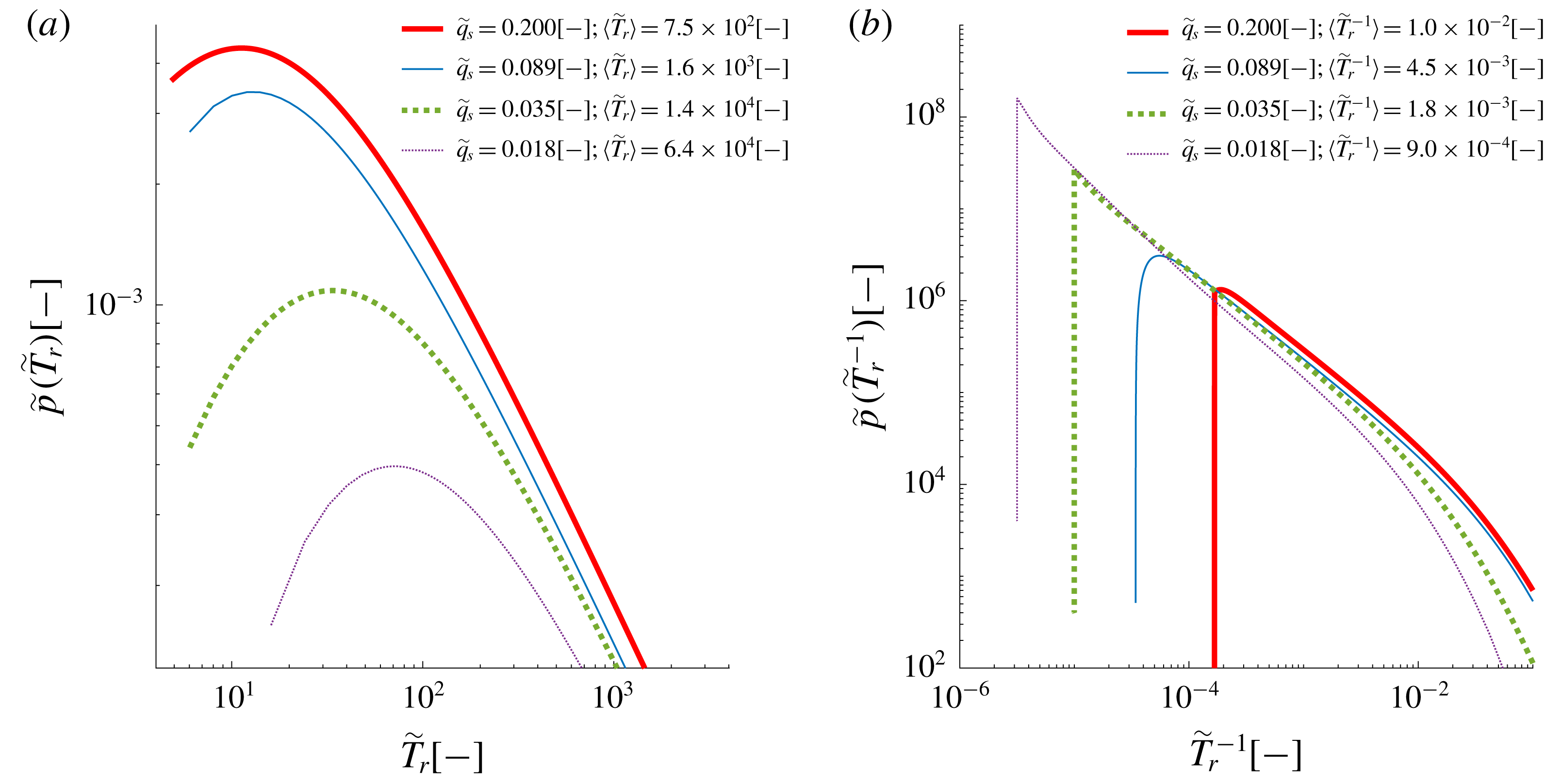
. We developed the solution for the four runs already considered in figure 3. The numerical results for
 $p(\tilde{T}_{r})$
, pursued through a recursive trial and error approach, are reported in figure 5(a), where both axes are logarithmic. We checked that the obtained
 $p(\tilde{T}_{r})$
satisfy all the constraints, i.e., to be positive with a unit integral, and to provide a mean of
 $\langle \tilde{T}_{r}^{-1}\rangle$
from (3.5) coinciding with the value from (3.7). In figure 5(a) each curve is tagged in the legend by the relevant values of
 $\tilde{q}_{s}$
and
 $\langle \tilde{T}_{r}\rangle$
. At a first sight the four
 $p(\tilde{T}_{r})$
curves display long and linear tails, in the log–log plots, features in common with power-law distributions (Voepel et al.
Reference Voepel, Schumer and Hassan2013). The mean resting-time decreases hyperbolically as
 $\tilde{q}_{s}$
increases. By increasing
 $\tilde{q}_{s}$
beyond the values featuring the nine performed runs, it would be approached the boundary between ordinary and collisionally suspended bed-load (Berzi & Fraccarollo Reference Berzi and Fraccarollo2013). This latter, intense sediment-transport regime is associated with the formation of an almost full layer of moving grains, which undergo mutual collisions and have little, almost null, rest-time. Hence, the Einstein conjecture, which applies to ordinary bed-load, breaks when the power of the stream is high enough to make the collisions between moving grains a dominant mechanism of the transport process.
Figure 5(b) displays the probability density functions
 $p({\tilde{T}_{r}}^{-1})$
for the four runs of (a), identified now by the values of
 $\tilde{q}_{s}$
and
 $\langle {\tilde{T}_{r}}^{-1}\rangle$
. The two panels of figure 5, together, provide a description of how the resting-times are distributed at the extremes, when
 $\tilde{T}_{r}$
tends to either 0 or
 $\infty$
.
(a) Probability density functions
 $p(\tilde{T}_{r})$
for four runs, identified by the values of
 $\tilde{q}_{s}$
and
 $\langle \tilde{T}_{r}\rangle$
. (b) Probability density functions
 $p({\tilde{T}_{r}}^{-1})$
for four runs, identified by the values of
 $\tilde{q}_{s}$
and
 $\langle {\tilde{T}_{r}}^{-1}\rangle$
.

5 Conclusions
Statistical information for ordinary bed-load transport have been obtained through an innovative experimental methodology based on image analysis applied where the bed is flat and made of well sorted particles. Two major findings are presented. The first one is a robust confirmation of Einstein’s assumption about average grain displacement, the distance run between two subsequent resting periods, which is shown to scale with only the grain-size at a given bed-slope. The second achievement consists of the probability density function of the grain resting-time inferred through a theoretical analysis of the raw data. These outcomes may be exploited in mechanical/statistical interpretation of the ordinary bed-load process or in the determination of associated features, e.g., the dispersion of pollution carried by the grains. Future analysis could address the role of the grain shape and of the bed-slope to see how our results can be extended to more general conditions.
Acknowledgements
The authors thank the associate editor, E. Guazzelli, and the anonymous reviewers for their commitment and guidance. The experiments have been performed with the vital help of two students, now engineers, A. Viviani and M. Verber. The technicians of the Hydraulic Laboratory of the University of Trento (A. Bampi, L. Forti, F. Sartori and P. Scarfiello) have, as always, provided the best setting to perform experimental works. K. Wlodarczyk (UBC, Vancouver) gave a generous English revision. Fruitful discussions have been had by the authors, at different stages of the work, with F. Ballio, D. Berzi, J. Campagnol, P. Frey, D. Furbish, J. Heyman, M. Larcher, S. Siboni and A. Radice.