


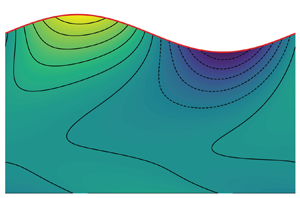



1. Introduction
The linear stability analysis of film-flow solutions predicts whether small disturbances grow or decay in the long term. This is particularly important in the dip-coating industrial process, where growing disturbances make the coating layer uneven, reducing the quality of the final product (Scriven Reference Scriven1988). The dip-coating process consists in applying a thin film of protective material over a solid substrate (Weinstein & Ruschak Reference Weinstein and Ruschak2004), with applications ranging from food industry (Suhag et al. Reference Suhag, Kumar, Petkoska and Upadhyay2020), e.g. coating composed of hydrophilic polymers dissolved in water (Jose, Pareek & Radhakrishnan Reference Jose, Pareek and Radhakrishnan2020), to corrosion-protection material, e.g. zinc coating in hot-dip galvanisation Kuklík & Kudlacek (Reference Kuklík and Kudlacek2016, Chapter 2). The substrate is coated by dipping and then withdrawing it from a liquid bath. Thereby, a liquid film forms on the substrate surface, which then solidifies into a protective layer. The thickness of this liquid film  $\bar {h}$ depends on the withdrawal velocity
 $U_p$ and the action of external control actuators.
In the uncontrolled case, known as free-coating or drag-out problem (Wilson Reference Wilson1982),  $\bar {h}$ depends on the ratio between viscous drag forces over surface tension forces at the free surface (capillary number
 $Ca=U_p\mu /\sigma$). For small Reynolds numbers (
 $Re$),
 $\bar {h}$ is given by the Landau–Levich–Derjaguin (LLD) solution for
 $Ca\ll 1$ (Derjaguin Reference Derjaguin1943; Landau & Levich Reference Landau and Levich1988) and by the Derjaguin (Reference Derjaguin1944) solution for
 $Ca\gg 1$. Both solutions define a monotonically non-decreasing relation between
 $\bar {h}$ and
 $U_p$ with thicker films for faster substrates. This contrasts with industrial needs aiming at thin films and fast substrates. To this end, in industrial lines, external actuators are used to remove the liquid excess from the film, e.g. impinging gas jets in the hot-dip galvanisation (Buchlin Reference Buchlin1997; Gosset & Buchlin Reference Gosset and Buchlin2006), allowing the thickness of the coating to be controlled regardless of the substrate velocity (Mendez et al. Reference Mendez, Gosset, Scheid, Balabane and Buchlin2021).
Tu & Ellen (Reference Tu and Ellen1986) and Gosset (Reference Gosset2007) studied the stability properties of the controlled liquid film, finding that the cutoff wavenumber is  $\propto \bar {h}^2Re^{1/2}Ca^{1/2}$. They solved the Orr–Sommerfeld eigenvalue problem with an asymptotic long-wave expansion at
 $O(k)$, valid for small Reynolds numbers (Benjamin Reference Benjamin1957; Yih Reference Yih1991). Other authors relied on integral boundary layer models to extend the analysis to larger
 $Re$ and short wavelengths. Ivanova et al. (Reference Ivanova, Pino, Scheid and Mendez2022) found that the cutoff wavenumber is
 $\propto \bar {h}^{3/2}Re^{1/2}Ca^{1/6}$, whereas Barreiro-Villaverde et al. (Reference Barreiro-Villaverde, Gosset, Lema and Mendez2023) showed that the film is more stable to three-dimensional (3-D) than to two-dimensional (2-D) disturbances. The disagreement between the Orr–Sommerfeld approximated long-wave solution and integral models suggests that a more thorough analysis of the full Orr–Sommerfeld eigenvalue problem is required, which is still absent from the literature.
An essential aspect of unstable perturbations is the physical mechanism leading to their growth. For a falling liquid film, asymptotic (Smith Reference Smith1990), vorticity and energy arguments (Kelly et al. Reference Kelly, Goussis, Lin and Hsu1989) showed that the motion induced by a small perturbation of the liquid film's free surface feeds the perturbation's energy by the work of shear stresses at the free surface. The extracted energy is stored in the disturbance's kinetic and potential surface tension energy. Understanding the growth mechanism in dip-coating conditions would shed some light on the role of substrate motion.
Another significant result given by the linear stability analysis is the threshold between absolutely and convectively unstable film flows (Kalliadasis et al. Reference Kalliadasis, Ruyer-Quil, Scheid and Velarde2011, Subsection 7.1.2). Knowing this threshold is essential for the design of control actions, which can affect the whole liquid film or only a part of it (Pier Reference Pier2003). The liquid film's impulse response can produce waves propagating along the flow direction (convectively unstable flow) or everywhere in the domain (absolutely unstable flow). Experiments (Liu, Paul & Gollub Reference Liu, Paul and Gollub1993), analytical and numerical works (Brevdo et al. Reference Brevdo, Laure, Dias and Bridges1999) proved that the falling film is convectively unstable, and the suspended film is absolutely unstable (Sterman-Cohen, Bestehorn & Oron Reference Sterman-Cohen, Bestehorn and Oron2017). Between these two extremes, a critical inclination angle defines the threshold between absolute and convective film flows (Brun et al. Reference Brun, Damiano, Rieu, Balestra and Gallaire2015; Scheid, Kofman & Rohlfs Reference Scheid, Kofman and Rohlfs2016; Pino, Scheid & Mendez Reference Pino, Scheid and Mendez2024). Likewise, a critical liquid-film thickness in dip coating defines the absolute/convective (AC) threshold (Pino, Mendez & Scheid Reference Pino, Mendez and Scheid2024). For small coating thicknesses, the entrainment due to the substrate motion sweeps the instabilities upwards; for large coating thicknesses, the gravitational effects push the instability downwards. For intermediate coating thicknesses, gravity and viscous entrainment should compensate for each other, resulting in a window of absolute instability. Knowing the position of this window in the parameters space is essential for the design of control laws, which can affect the liquid film downstream, upstream or everywhere. Despite its implications, this remains an open question that has not yet been answered and which we address theoretically in this paper.
This work studies the stability of controlled and uncontrolled liquid-film-flow solutions over a substrate moving against gravity. Given the wide variety of coating liquids, going from vegetable oils (Sharmin et al. Reference Sharmin, Zafar, Akram, Alam and Ahmad2015) to liquid metals, this analysis focuses on four liquids with a ratio of surface tension forces to inertial forces (Kapitza number  $Ka$) in the range between
 $Ka\sim O(1)$ and
 $Ka\sim O(10^4)$. We solve the Orr–Sommerfeld eigenvalue problem via the Chebyshev–Tau spectral method (Ortiz Reference Ortiz1969; Lanczos Reference Lanczos1988; Johnson Reference Johnson1996, Chapter VII) and compare the neutral stability conditions for different values of non-dimensional film thickness. Based on the Orr–Sommerfeld solution, we calculate the components of the energy balance equations and compute the AC threshold. Although this holds in linear analysis, it is worth noting that nonlinear mechanisms may affect the spanwise development of initial perturbations, as observed by Barreiro-Villaverde et al. (Reference Barreiro-Villaverde, Gosset, Lema and Mendez2023) in a coating film and by Ledda et al. (Reference Ledda, Balestra, Lerisson, Scheid, Wyart and Gallaire2021) in an inverted film with calcium carbonate deposition.
The rest of the article is organised as follows. The problem set-up is described in § 2, and a description of the scaling quantities is given in § 2.1. Section 2.2 reports the governing equations, the eigenvalue problem formulation and the instability energy balance equation. The numerical implementation is reported in § 3 with methods used to solve the Orr–Sommerfeld problem, calculate the energy balance equation and search the AC threshold. Results are presented in § 5 with the stability curves, the perturbation's energy budget and the AC instability threshold. Conclusions and perspectives are given in § 6.
2. Problem description
We consider a 2-D liquid film with density  $\rho$, dynamic viscosity
 $\mu$, kinematic viscosity
 $\nu$ and surface tension
 $\sigma$, over a vertical substrate moving against gravity
 $g$ at constant speed
 $U_{p}$. Table 1 reports the physical properties of the four liquids considered in this work: liquid zinc, water, water–glycerol solution (glycerol concentration 45 % by volume) and corn oil. These cover a broad range of conditions encountered in dip or slot coating (Gosset, Mendez & Buchlin Reference Gosset, Mendez and Buchlin2019; Barreiro-Villaverde et al. Reference Barreiro-Villaverde, Gosset, Lema and Mendez2023). Figure 1(a) shows the fixed reference system (
 $\mathscr {O}xy$) with
 $x$ aligned with the plate and pointing in the direction of the gravitational acceleration,
 $y$ along the wall-normal direction towards the free-surface, with the origin
 $\mathscr {O}$ on an arbitrary point of the substrate, given the translational invariance of the problem.
Properties of the four liquids considered in the analysis (density, dynamic viscosity and surface tension from left to right), Kapitza number ( $Ka$) and range of Reynolds numbers (
 $Re$) for substrate velocity
 $U_{p}\in [0.1,3]$ m s
 $^{-1}$ for the four liquids considered in the analysis.

(a) Schematic of the investigated configuration with a vertical liquid film over a substrate moving with velocity  $U_p$, where the dimensional liquid-film height
 $h$ can be scaled by
 $h_{ref}$ and decomposed into a dimensionless base state
 $\bar {h}$ and a dimensionless harmonic perturbation
 $\tilde {h}$ of
 $O(1)$, with
 $\varepsilon \ll 1$. Liquid-film response (red continuous curve) of a (b) convectively and (c) absolutely unstable base state solution to an initial pulse (black dashed line).

2.1. Scaling quantities
For a given liquid, the two control parameters of the systems are the substrate velocity  $U_{p}$ and the liquid-film thickness
 $h$. We define as reference velocity
 $U_{p}$ and as reference length the film thickness resulting from the steady-state viscous-gravity balance (see Mendez et al. Reference Mendez, Gosset, Scheid, Balabane and Buchlin2021):
 \begin{equation} u_{ref} = U_{p}, \quad h_{ref} = \sqrt{\frac{\nu U_{p}}{g}}, \end{equation}
where the subscript ‘ ${ref}$’ denotes reference quantities. We define the capillary length
 $\ell _{c}$, relating gravity and surface tension, and the viscous length
 $\ell _{\nu }$, relating gravity and viscosity, as
 \begin{equation} \ell_{c} = \sqrt{\frac{\sigma}{\rho g}},\quad \ell_{\nu}=\sqrt[3]{\frac{\nu^2}{g}}. \end{equation}
Based on velocity and length scales in (2.1), the dependent and independent variables are scaled accordingly:
 \begin{gather} (u,v)\rightarrow u_{ref}(\hat{u},\hat{v}), \quad (x,y)\rightarrow h_{ref}(\hat{x},\hat{y}), \quad h\rightarrow h_{ref}\hat{h}, \end{gather}
 \begin{gather}t\rightarrow \frac{h_{ref}}{u_{ref}}\hat{t},\quad p\rightarrow p_{\infty} + \rho g h_{ref}\hat{p}, \end{gather}
where the hat  $\hat {{\cdot }}$ denotes the non-dimensional quantities and
 $p_{\infty }$ the atmospheric pressure. To make the non-dimensional thickness
 $\hat {h}$ independent of
 $U_{p}$ and to have a clearer understanding of the role of the control parameters, we introduce another non-dimensional film thickness
 $\breve {h}$ based on
 $\ell _{\nu }$:
 \begin{equation} h\rightarrow \ell_{\nu}\breve{h}. \end{equation}
The non-dimensional groups arising from our scaling are the Reynolds number:
 \begin{equation} Re = \frac{u_{ref}h_{ref}}{\nu} = \sqrt{\frac{U_{p}^3}{g\nu}}, \end{equation}
which is equivalent to the Froude number defined as
 \begin{equation} F = \frac{u_{ref}^2}{g h_{ref}} = \sqrt{\frac{U_{p}^3}{g\nu}}. \end{equation}
This means that  $Re$ represents the ratio of inertia over viscous forces and the ratio between inertia and gravitational forces. The other non-dimensional group is the inverse of the capillary number defined as the ratio between surface tension and gravity:
 \begin{equation} Ca^{{-}1} = \frac{\sigma}{u_{ref} \mu} = \frac{Ka}{Re^{2/3}},\end{equation}
where  $Ka$ is the Kapitza number defined as
 \begin{equation} Ka = \frac{\sigma}{\rho g^{1/3} \nu^{4/3}}. \end{equation}
Based on these non-dimensional groups, the non-dimensional capillary and viscous wavenumbers read
 \begin{equation} k_{\ell_{c}} = \frac{2{\rm \pi}}{\hat{\ell}_{c}} = \frac{2{\rm \pi} Re^{1/3}}{Ka^{1/2}}, \quad k_{\ell_{\nu}} = \frac{2{\rm \pi}}{\hat{\ell}_{\nu}} = 2{\rm \pi} Re^{1/3}. \end{equation}
Using the scaling in (2.1), the Derjaguin (Reference Derjaguin1944) flat film solution corresponds to  $\hat {h}=1$ and the LLD solution (Derjaguin Reference Derjaguin1943; Landau & Levich Reference Landau and Levich1988; Snoeijer et al. Reference Snoeijer, Ziegler, Andreotti, Fermigier and Eggers2008) corresponds to
 \begin{equation} {\mathop{h}\limits^{\circ}} = 0.945Ca^{1/6}. \end{equation}
2.2. Mathematical formulation
The liquid film is governed by the incompressible 2-D Navier–Stokes equations, with a velocity vector  $\boldsymbol {v}=(u(x,y),v(x,y))$ and a pressure field
 $p(x,y)$. The equations are accompanied by the non-slip condition at the substrate
 $\boldsymbol {v}(x,y=0)=(-U_p,0)$ and a set of kinematic and dynamic boundary conditions at the free surface (
 $y=h$), accounting for the continuity of the interface, and the normal and tangential force balance (see Kalliadasis et al. Reference Kalliadasis, Ruyer-Quil, Scheid and Velarde2011, Chapter 2). The non-dimensional steady-state solutions (base states) are given by a flat interface (
 $\hat {h}=\bar {h}$) and the following velocity and pressure fields:
 \begin{equation} \bar{u}(\hat{y}) ={-}\tfrac{1}{2}\hat{y}^2 + \bar{h}\hat{y} - 1,\quad \bar{v}(\hat{y}) = 0,\quad \bar{p}(\hat{y}) = 0, \end{equation}
where  $\bar {{\cdot }}$ denotes the base state quantities. The balance between wall shear stress and gravity, along with the imposed velocity at the boundary, produce a non-monotonic relation between non-dimensional flow rate
 $\hat {q}=q/(u_{ref}h_{ref})$ and
 $\hat {h}$:
 \begin{equation} \bar{q} = \tfrac{1}{3}\bar{h}^3 - \bar{h}. \end{equation}
As shown in figure 2(a), this relation entails two branches of steady-state solutions: a thin one ( $\bar {h} < 1$) (orange area) and a thick one (
 $\bar {h} > 1$) (blue area) with the Derjaguin's solution (red dot) and the solution
 $\bar {h}=\sqrt {3}$ (green square) defining the limit of zero net flow rate, above which we enter the falling film regime, i.e. for
 $\bar {h}>\sqrt {3}$. Figure 2(b) shows the non-dimensional streamwise velocity profile
 $\bar {u}(\hat {y})$ associated with Dejarguin's solution (continuous red line) and the thin (orange) and thick (blue) film solution (lines with markers).
(a) Relation between the non-dimensional liquid film  $\hat {h}$ and flow rate
 $\hat {q}$ with the Derjaguin solution (red circle), the maximum thickness
 $\hat h=\sqrt {3}$ (green square) and the thin film (orange shadowed) and thick film (blue shadowed) regions with (b) the associated velocity profiles.

To analyse the stability of the base states given by (2.11), we decompose the dependent variables as follows:
 \begin{equation} \hat{u} = \bar{u} + \varepsilon\tilde{u},\quad \hat{v}= \bar{v} + \varepsilon\tilde{v},\quad \hat{p} = \bar{p} + \varepsilon\tilde{p},\quad \hat{h} = \bar{h} + \varepsilon\tilde{h}, \end{equation}
where  $\tilde {{\cdot }}$ represents the perturbations of O(1) and
 $\varepsilon \ll 1$ a small parameter. Inserting (2.13) into the governing equations with the kinematic and dynamic boundary conditions and collecting the term at O
 $(\varepsilon )$ yields the linearised perturbation (Navier–Stokes) equations:
 \begin{gather} \partial_{\hat{x}}\tilde{u} + \partial_{\hat{y}}\tilde{v} = 0, \end{gather}
 \begin{gather}Re(\partial_{\hat{t}}\tilde{u} + \bar{u}\partial_{\hat{x}}\tilde{u} + \tilde{v} D\bar{u}) ={-}\partial_{\hat{x}}\tilde{p} + \nabla^2\tilde{u}, \end{gather}
 \begin{gather}Re(\partial_{\hat{t}}\tilde{v} + \bar{u}\partial_{\hat{x}}\tilde{v}) ={-}\partial_{\hat{y}}\tilde{p} + \nabla^2\tilde{v}, \end{gather}
where  $D({\cdot })=\partial _{\hat {y}}({\cdot })$ is the wall-normal differential operator. The boundary conditions at the substrate (
 $\hat {y}=0$) reads
 \begin{equation} \tilde{u}=\tilde{v}=0,\end{equation}
and, at the free surface ( $\hat {y}=\hat {h}$),
 \begin{gather} \tilde{v} = \partial_{\hat{t}}\tilde{h} + \bar{u}\partial_{\hat{x}}\tilde{u}, \end{gather}
 \begin{gather}\tilde{p} = 2\partial_{\hat{y}}\tilde{v} - Ca^{{-}1}\partial_{\hat{x}\hat{x}}\tilde{h}, \end{gather}
 \begin{gather}\tilde{h} = \partial_{\hat{y}}\tilde{u} + \partial_{\hat{x}}\tilde{v}. \end{gather}
We concatenate the streamwise  $\tilde {u}$ and cross-stream
 $\tilde {v}$ perturbations, by recasting (2.14) in terms of the stream function
 $\varPsi$ defined as
 \begin{equation} \tilde{u} = \partial_{\hat{y}}\varPsi, \quad \tilde{v} ={-}\partial_{\hat{x}}\varPsi, \end{equation}
and assuming a normal mode solution of the form
 \begin{equation} \varPsi = \varphi(\hat{y}) \exp({\rm i}(k\hat{x} - \omega\hat{t})), \quad \tilde{h} = \eta\exp({\rm i}(k\hat{x} - \omega\hat{t})), \end{equation}
where  $\varphi (\hat {y}) = \varphi _r(\hat {y}) + {\rm i}\varphi _i(\hat {y})$ and
 $\eta$ are the amplitudes of the stream function and the film thickness, respectively,
 $k=k_r + {\rm i}k_i$ is the wavenumber,
 $\omega = \omega _r + {\rm i}\omega _i$ the angular frequency, and
 $c=c_r + {\rm i}c_i=\omega /k$ is the perturbation's complex phase speed. This yields the following Orr–Sommerfeld eigenvalue problem:
 \begin{equation} \boldsymbol{OS}(k,c,Re)\varphi(\hat{y}) = [\boldsymbol{A}(k,Re) - c\boldsymbol{B}(k,Re)]\varphi(\hat{y})=0, \end{equation}
where  $\boldsymbol {A}(k,Re)$ is given by
 \begin{equation} \boldsymbol{A}(k,Re) = (D^2-k^2)^2 - {\rm i}\,Re\, k[\bar{u}(D^2-k^2)+1] \end{equation}
and  $\boldsymbol {B}(k,Re)=\partial _c\boldsymbol {OS}(k,c,Re)$ is given by
 \begin{equation} \boldsymbol{B}(k,Re) ={-}{\rm i}\,Re \,k(D^2 -k^2), \end{equation}
with boundary conditions  $\boldsymbol {OS}_{BC}\varphi |_{0,\hat {h}}=0$ defined as
 \begin{gather} \varphi(0)=D\varphi(0)= 0, \end{gather}
 \begin{gather}\eta = \varphi(\hat{h})/(c-a), \end{gather}
 \begin{gather}{}[(D^2 - 3k^2) + {\rm i} \,Re \,k (c -a)]D\varphi(\hat{h}) - {\rm i}\eta \,Ca^{{-}1} \,k^3 = 0, \end{gather}
 \begin{gather}(D^2 + k^2)\varphi(\hat{h}) - \eta = 0, \end{gather}
where  $a = \bar {u}(\bar {h}) = (\bar {h}^2/2-1)$ is the base-state velocity at the interface.
The solution of the eigenvalue problem sets a relation between the wavenumber  $k$ and angular frequency
 $\omega$. This is known as the dispersion relation and depends on three parameters:
 \begin{equation} \mathscr{D}(\omega,k; Re, Ka, \bar{h})= 0. \end{equation}
These solutions are linked to the system's response to a local impulse, known as Green's function (Brevdo et al. Reference Brevdo, Laure, Dias and Bridges1999; Schmid & Henningson Reference Schmid and Henningson2001, pp. 270–271). It can be shown that these are the system's poles (Charru Reference Charru2011, p. 97) and, thus, control whether a disturbance grows or vanishes.
The analysis of poles for varying  $\omega$ with a fixed
 $k$ is known as a temporal analysis, whereas the analysis of poles for varying
 $k$ and fixed
 $\omega$ is known as a spatial analysis. The images of any straight lines
 $k_i=\textit {C}$, where
 $\textit {C}$ is an arbitrary constant, are called temporal branches in the complex frequency space, whereas the images of any straight line
 $\omega _i=\textit {E}$, where
 $\textit {E}$ is an arbitrary constant, are called spatial branches in the complex wavenumber space (Kupfer, Bers & Ram Reference Kupfer, Bers and Ram1987). The points of intersection of spatial branches are called spatial branch points.
For a real  $k$, a base state is classified as temporally stable or unstable, depending on the value of the growth rate (
 $\omega _i$): a state is unstable if
 $\omega _i>0$, as this results in the unbounded temporal growth of infinitesimal perturbation, whereas it is stable if
 $\omega _i<0$, as this results in the return of the perturbed liquid film to its steady-state equilibrium conditions for all
 $k$. The locus of points with zero growth rate (
 $\omega _i=0$) corresponds to the neutral curve, with neither amplified nor damped perturbations.
A base state is absolutely unstable if the solution with zero group velocity  $c_g=\partial \omega /\partial k=0$ has
 $\omega _i>0$ (Gaster Reference Gaster1968; Charru Reference Charru2011). The condition
 $c_g=0$ is equivalent to
 $\partial \omega _r/\partial k_r=\partial \omega _i/\partial k_r=0$ or, because of the Cauchy–Riemann relation, to
 $\partial \omega _i/\partial k_i=\partial \omega _r/\partial k_i=0$. Since both
 $\omega _r$ and
 $\omega _i$ must also satisfy the Laplace equation in the wavenumber domain
 $k$ for a differentiable (holomorphic)
 $\omega (k)$, this implies that the condition
 $c_g=\partial \omega /\partial k=0$ corresponds to a saddle point in the wavenumber domain
 $k$. However, not all saddle points are admissible; we return to this point in § 3.2.
3. Methodology
3.1. Numerical solution of the eigenvalue problem
Before presenting the numerical methods used to solve the Orr–Sommerfeld problem, we remove  $\eta$ from the boundary conditions (2.22), substituting the kinematic condition (2.22b) into the shear stress balance (2.22d) and the original shear stress balance (2.22d) into the normal stress balance (2.22c) (Pelisson Chimetta, Hossain & de Moraes Franklin Reference Pelisson Chimetta, Hossain and de Moraes Franklin2018). The Orr–Sommerfeld eigenvalue problem (2.19) with the modified boundary conditions is solved using the Chebyshev–Tau spectral method (Johnson Reference Johnson1996; Canuto et al. Reference Canuto, Hussaini, Quarteroni and Thomas2012, Section. 3.1). The eigenfunction
 $\varphi (\hat {y})$ is approximated with a combination of
 $N+1$ Chebyshev polynomials of the first kind, with the coefficients
 $a_i$ being collected in the vector
 $\boldsymbol {\phi }=[a_0,a_1,\ldots,a_N]^{\rm T}$. The approximated eigenfunction is introduced in (2.19), and the residual is projected onto another base of Chebyshev polynomials of the first kind. This results in an algebraic system of
 $N+1$ equations representing a generalised eigenvalue problem with eigenvector
 $\phi$ and eigenvalue
 $c$:
 \begin{equation} (\mathsf{{A}}(Re,k) - c\mathsf{{B}}(Re,k))\phi = 0, \end{equation}
with matrices  $\mathsf{{A}}$ and
 $\mathsf{{B}}$ representing the discretisation of the operators
 $\boldsymbol {A}$ in (2.20) and
 $\boldsymbol {B}$ in (2.21). Replacing the last four rows of the system in (3.1) with the modified boundary conditions (Boyd Reference Boyd2001, Section 6.4) leads to the generalised eigenvalue problem:
 \begin{equation} \hat{A}(Re,k)\phi = c \hat{B}(Re,k)\phi, \end{equation}
with  $\hat {A}$ and
 $\hat {B}$ representing matrices
 $\mathsf{{A}}$ and
 $\mathsf{{B}}$ in (3.1) with the enforced boundary conditions. The eigenvalue problem is solved using Python's function numpy.linalg.eig. The approximation error decreases as the magnitude of the four
 $\tau$ coefficients is reduced Lanczos (Reference Lanczos1988, Chapter 7, § 12).
To cope with the spurious eigenvalues (Dawkins, Dunbar & Douglass Reference Dawkins, Dunbar and Douglass1998; Bourne Reference Bourne2003), we solve (3.2) for  $N=20$ and
 $N=80$, retaining the eigenvalues whose difference in magnitude, using the Euclidean norm (
 $\|{\cdot }\|$), is below 0.1 (Gardner, Trogdon & Douglass Reference Gardner, Trogdon and Douglass1989). Among these, that with the largest growth rate
 $\omega_{i1}^{1}=c_{i1}^{1}/k$ (most unstable) is selected. To further improve the computational accuracy of the associated eigenvector
 $\phi_{1}^{1}$, we run 10 iterations of the inverse power method (Trefethen & Bau Reference Trefethen and Bau2022, Lecture 27):
 \begin{equation} \phi^{j+1} = \frac{(C - I/c_1)^{{-}1}\phi^{\{j\}}_{1}}{||(C - I/c_1)^{{-}1}\phi_1^{\{j\}}||}, \end{equation}
where  $j\in \{1,2,\ldots,9\}$ is the iteration count and
 $C=\hat {A}^{-1}\hat {B}$. We defined
 $C$ in this way, with the inverse of
 $\hat {A}$ rather than the inverse of
 $\hat {B}$, because
 $\hat {B}$ is always singular.
Given  $Ka$ and
 $\hat {h}$, to compute the neutral stability curves in the
 $k$–
 $Re$ space with
 $k\in \mathbb {R}$, we start from the long-wave most-unstable mode (
 $(\phi_1,c_1)$ with the largest
 $c_i$), with
 $k^{\{1\}}=3.5\times 10^{-6}$, and we march it along the discrete
 $k$ axis running 20 iterations of Rayleigh quotient iteration at every point
 $k^{\{j\}}$ and collecting the values of
 $c^{\{j\}}$:
 \begin{equation} \phi_1^{\{j+1\}} = \frac{(C - I/c_1^{(j)})\phi_1^{\{j\}}}{||(C - 1/c_1^{\{j\}})^{{-}1}\phi_1^{\{j\}}||}, \quad I/c_1^{\{j+1\}} = \frac{\phi_1^{*\{j+1\}}C\phi_1^{\{j+1\}}}{\phi_1^{*\{j+1\}}\phi_1^{\{j+1\}}}, \end{equation}
where  ${\cdot }^*$ denotes complex conjugate. Thereby, converting
 $c_i$ into
 $\omega _i$, we find the growth rate as a function of
 $k$. The zero of this curve
 $k_f$ (
 $k\in \mathbb {R}:\omega _i(k)=0\wedge k\neq 0$), also known as the cutoff frequency, belongs to the neutral curve. The neutral curve is constructed by repeating this procedure varying
 $Re$.
3.2. Numerical method for zero group-velocity perturbation
To assess whether a base state is absolutely or convectively unstable, we follow Brigg's method (outlined in Schmid & Henningson Reference Schmid and Henningson2001, Subsection 7.2.2). This consists of mapping the complex  $k$ space into the complex
 $\omega$ space, identifying the saddle points, and checking a posteriori if these respect the causality condition using the collision criterion (Briggs Reference Briggs1964; Huerre & Monkewitz Reference Huerre and Monkewitz1985; Thual, Thual & Dewitte Reference Thual, Thual and Dewitte2013; Avanci, Rodríguez & Alves Reference Avanci, Rodríguez and Alves2019). According to this criterion, the only valid saddle points arise as spatial branch points, pinching two spatial branches coming from the positive and negative half-planes of the complex wavenumber space. Depending on the value of the growth rate in these points, the base state is convectively (
 $\omega _i<0$) or absolutely (
 $\omega _i>0$) unstable.
Given a set of parameters ( $Re$,
 $Ka$,
 $\hat {h}$), we explore a portion of the complex wavenumber space
 $k_i\in [k_{i_{min}},k_{i_{max}}]$ and
 $k_r\in [k_{r_{min}},k_{r_{max}}]$, discretised with a uniform mesh of
 $M\times M$ elements with spacing
 $\Delta k_i$ and
 $\Delta k_r$. Starting from the most-unstable mode
 $(\phi_1,c_1)$, obtained solving the Orr–Sommerfeld problem (3.2) for a given pair (
 $k_r^{\{1\}},k_i^{\{1\}}$), we march over the discretised wavenumber space running 20 iterations of Rayleigh quotient iteration (3.4) at every point (
 $k_r^{\{j\}},k_i^{\{j\}}$) and collecting the values of
 $c^{\{j\}}$. The solution at one point of the grid serves as a starting point for the computation of the solution in the adjacent one. We march over the wavenumber space with a spiral matrix algorithm to avoid two consecutive steps falling outside the iterative method's convergence region. Given the computed mapping
 $\omega _r(k_r,k_i),\omega _i(k_r,k_i)$, we calculate the saddle point location using numerical differentiation and checking the collision condition.
Figure 3(a) presents an example of the mapping, with  $\omega _i$ colour plot and contour map as a function of
 $k$, along with the position of the saddle point (red point). To check whether the collision criterion is satisfied, we check the position of the saddle point in the complex
 $\omega$ space. Figure 3(b) shows the saddle point position (red dot) in the complex
 $\omega$ space and the temporal branches of the first five modes (coloured lines), sorted by ascending values of
 $\omega _i$, along the path
 $k_i=0$. The collision criterion is respected if the saddle point is surmounted by an odd number of spatial branches (Kupfer et al. Reference Kupfer, Bers and Ram1987; Suslov Reference Suslov2006).
Position of the saddle point (red dot) for the zinc with  $\hat {h}=0.8885$,
 $Re=30$ (a) in the complex
 $k$ space with the colourmap of
 $\omega _i$ and (b) in the complex frequency space with the cusp (black dashed line) and the spatial branches of the first four modes (coloured lines), sorted by ascending values of
 $\omega _i$, obtained solving the Orr–Sommerfeld problem along the path
 $k_i=0$ in the complex wavenumber space.

To determine the AC instability threshold (saddle point with  $\omega _i=0$), we explore the parameter spaces (
 $Ka$–
 $Re$) and (
 $\hat {h}$–
 $Re$). We fix
 $Re$ and run a line search along the other parameter. A detailed pseudocode description is reported in Appendix A.
4. Energy balance and mechanism of the unstable perturbation
To understand the onset mechanism of unstable perturbations, we solve the linearised Navier–Stokes equations via a long-wave asymptotic expansion up to  $O(k^2)$ in § 4.1. In addition, to gain a deeper insight into the growth mechanism of unstable perturbations for any
 $k$, we derive the kinetic energy balance for the perturbations in § 4.2.
4.1. Mechanism of long-wave instability in a moving reference frame
We consider a solution of (2.14) with boundary conditions (2.15) and (2.16) in the form of normal modes given by
 \begin{gather} \tilde{u} = \acute{u}(\hat{y})\exp({\rm i}k(\hat{x} - c\hat{t})), \quad \tilde{v} = \acute{v}(\hat{y})\exp({\rm i}k(\hat{x} - c\hat{t})), \end{gather}
 \begin{gather}\tilde{h} = \eta\exp({\rm i}k(\hat{x} - c\hat{t})), \quad \tilde{p} = \acute{p}(\hat{y})\exp({\rm i}k(\hat{x} - c\hat{t})), \end{gather}
where the  $\acute {{\cdot }}$ denotes the amplitudes. We consider a reference system moving with the substrate velocity
 $U_p$ (
 $\hat {u}=-1$), with the change of variables:
 \begin{equation} \acute{u}_m(\hat{y}) = \acute{u}(\hat{y}) + 1, \quad c_m = c + 1, \quad \bar{u}_m(\hat{y}) = \bar{u}(\hat{y}) + 1 ={-}\frac{y^2}{2} + \hat{h}\hat{y}, \end{equation}
where  $\acute {u}_m$,
 $c_m$ and
 $\bar {u}_m$ are the streamwise velocity amplitude, the phase speed and the base state velocity in the moving reference frame. We seek an approximated solution via long-wave expansion of the amplitudes and the phase speed up to
 $O(k)$ (Benjamin Reference Benjamin1957; Yih Reference Yih1963; Smith Reference Smith1990):
 \begin{gather} \acute{u}_m = \acute{u}_{m0} + \acute{u}_{m1}k + O(k^2), \quad \acute{v} = \acute{v}_0 + \acute{v}_1k + O(k^2),\quad\acute{p} = \acute{p}_0 + \acute{p}_1k + O(k^2), \end{gather}
 \begin{gather}\eta = \eta_0 + \eta_1k + O(k^2),\quad c_m = c_{m0} + c_{m1}k + O(k^2), \end{gather}
with the normalisation  $\eta _0 = 1$ and
 $\eta _1=0$. Collecting the terms at
 $O(1)$ gives the system
 \begin{equation} D\acute{v}_0(\hat{y}) = 0, \quad \acute{v}_0(\hat{y})D\bar{u}_m(\hat{y})Re = D^2 \acute{u}_{m0}(\hat{y}), \quad D\acute{p}_0(\hat{y}) = D^2 \acute{v}_0(\hat{y}), \end{equation}
with boundary conditions
 \begin{gather} \acute{u}_{m0}(0) = 0, \quad \acute{v}_0(0) = 0, \end{gather}
 \begin{gather}\acute{p}_0(\hat{h}) = 2\acute{v}_0(\hat{h}), \quad \acute{v}_0(\hat{h}) = 0 \quad D\acute{u}_{m0}(\hat{h})=1. \end{gather}
At  $O(k)$, we obtain the system
 \begin{gather} \acute{v}_1(\hat{y})+{\rm i} (\acute{u}_{m0}(\hat{y})-1) = 0, \end{gather}
 \begin{gather}-Re(\acute{u}_{m0}(\hat{y})-1) (c_{m0}-\bar{u}_m(\hat{y})+1)+\acute{p}_0(\hat{h})-{\rm i}\,Re\, \acute{v}_1(\hat{y}) D\bar{u}_m(\hat{y})+{\rm i} D^2\acute{u}_{m1}(\hat{y}) = 0, \end{gather}
 \begin{gather}-{\rm i} c_{m0} \,Re \,\acute{v}_0(\hat{y})+D\acute{p}_1(\hat{y})+{\rm i}\,Re\, \bar{u}_m(\hat{y}) \acute{v}_0(\hat{y})-{\rm i}\,Re\, \acute{v}_0(\hat{y})-D\acute{v}_1(\hat{y}) = 0, \end{gather}
with the boundary conditions
 \begin{gather} \acute{u}_1(0)=0\quad \acute{v}_1(0)=0, \end{gather}
 \begin{gather}\acute{v}_1(\hat{h}) ={-}{\rm i} (c_{m0} - \bar{u}_m(\hat{h})+1), \end{gather}
 \begin{gather}\acute{p}_1(\hat{y})-2 D\acute{v}_1(\hat{h})=0, \quad D\acute{u}_{1m}(\hat{h})+{\rm i} \acute{v}_0(\hat{h}) = 0 . \end{gather}
The solution of these systems is presented in § 5.2.
4.2. Energy balance of the perturbation
To study the instability mechanism, we analyse the contributions to the perturbation's kinetic energy equation as in Kelly et al. (Reference Kelly, Goussis, Lin and Hsu1989) and Lin (Reference Lin1970). This equation is obtained by summing up the product of (2.14b) by  $\tilde {u}$ and of (2.14c) by
 $\tilde {v}$, averaging over a wavelength
 $\lambda$, integrating over the liquid-film thickness
 $\hat {h}$ and then using (2.14a) and the boundary conditions (2.15) and (2.16c) to obtain
 \begin{equation} {\rm RKINE} + {\rm SURTE} = {\rm SHEST} + {\rm REYNS} + {\rm DISSI}, \end{equation}
with
 \begin{gather} {\rm RKINE} =\frac{1}{2\lambda}\frac{{\rm d}}{{\rm d}t}\int_{0}^{\lambda}\int_{0}^{\hat{h}}(\tilde{u}^2 + \tilde{v}^2)\,{\rm d}\hat{y}\,{\rm d}\hat{x}, \end{gather}
 \begin{gather}{\rm SURTE} ={-}\frac{Ca^{{-}1}}{Re\,\lambda}\int_{0}^{\lambda}[\tilde{v}|_{\hat{h}}(\partial_{\hat{x}\hat{x}}\tilde{h})]\, {\rm d}\hat{x}, \end{gather}
 \begin{gather}{\rm SHEST} = \frac{1}{Re\,\lambda}\int_{0}^{\lambda}\tilde{u}|_{\hat{h}}(\partial_{\hat{y}}\tilde{u}|_{\hat{h}} + \partial_{\hat{x}}\tilde{v}|_{\hat{h}})\, {\rm d}\hat{x}, \end{gather}
 \begin{gather}{\rm REYNS} ={-}\frac{1}{\lambda}\int_{0}^{\lambda}\int_{0}^{\hat{h}}\tilde{u}\tilde{v}D\bar{u}\,{\rm d}\hat{y}\,{\rm d}\hat{x}, \end{gather}
 \begin{gather}{\rm DISSI} = {\rm DISSI}_1 + {\rm DISSI}_2 + {\rm DISSI}_3. \end{gather}
The terms on the left-hand side represent the energy stored in the perturbation in the form of kinetic (RKINE) and surface tension potential (SURTE) energies. The terms on the right-hand side represent the energy extracted from the base state through the work of shear stress at the interface (SHEST), Reynolds stress (REYNS) and dissipative viscous effects (DISSI). DISSI encompass the contribution of extensional ( ${\rm DISSI}_1$ and
 ${\rm DISSI}_3$) and shear terms (
 ${\rm DISSI}_2$), given by
 \begin{gather} {\rm DISSI}_1 ={-}\frac{1}{Re\,\lambda}\int_{0}^{\lambda}\int_{0}^{\hat{h}} 2(\partial_{\hat{x}}\tilde{u})^2 \,{\rm d}\hat{y}\,{\rm d}\hat{x}, \end{gather}
 \begin{gather}{\rm DISSI}_2 ={-}\frac{1}{Re\,\lambda}\int_{0}^{\lambda}\int_{0}^{\hat{h}} \upsilon^2 \,{\rm d}\hat{y}\,{\rm d}\hat{x}, \end{gather}
 \begin{gather}{\rm DISSI}_3 ={-}\frac{1}{Re\,\lambda}\int_{0}^{\lambda}\int_{0}^{\hat{h}} 2(\partial_{\hat{y}}\tilde{v})^2\,{\rm d}\hat{y}\,{\rm d}\hat{x}, \end{gather}
where  $\upsilon = \partial _{\hat {y}}\tilde {u} + \partial _{\hat {x}}\tilde {v}$ is proportional to the strain rate. The perturbation quantities are given by
 \begin{gather} \tilde{u} = (D\varphi_r\cos(\theta) - D\varphi_i\sin(\theta))E, \end{gather}
 \begin{gather}\tilde{v} = k(\varphi_i\cos(\theta) + \varphi_r\sin(\theta))E, \end{gather}
 \begin{gather}(\partial_{\hat{y}}\tilde{u} + \partial_{\hat{x}}\tilde{v}) = [(D^2 + k^2)(\varphi_r\cos(\theta) - \varphi_i\sin(\theta)]E, \end{gather}
 \begin{gather}\tilde{\omega} = [(D^2 -k^2)(\varphi_r\cos(\theta) - \varphi_i\sin(\theta)]E, \end{gather}
 \begin{gather}\tilde{h} = (\eta_r\cos(\theta) - \eta_i\sin(\theta))E, \end{gather}
with
 \begin{equation} \theta = k(x - c_rt), \quad E=\exp(kc_it), \quad \tilde{\omega} = \partial_{\hat{y}}\tilde{u} - \partial_{\hat{x}}\tilde{v}, \end{equation}
where  $\tilde {\omega }$ is the perturbation vorticity.
Using the kinematic condition (2.22b), the real  $\eta _r$ and imaginary
 $\eta _i$ parts of surface deflection are given by
 \begin{gather} \eta_r = (\varphi_r(\hat{h})\hat{c} + \varphi_i(\hat{h})c_i)/(\hat{c}^2 + c_i^2), \end{gather}
 \begin{gather}\eta_i = (\varphi_i(\hat{h})\hat{c} - \varphi_r(\hat{h})c_i)/(\hat{c}^2 + c_i^2), \end{gather}
where  $\hat {c} = c_r - a$. To have an accurate computation of the terms in (4.8a), we calculate the integral along
 $\hat {x}$ analytically and along
 $\hat {y}$ numerically, using the Simpson's rule over a grid of
 $10^4$ equispaced points in the range
 $[0,\hat {h}]$ such that the difference in magnitude between the right-hand side and the left-hand side of (4.8a) is below
 $1\,\%$ of the kinetic energy (RKINE) (Lin, Lian & Creighton Reference Lin, Lian and Creighton1990).
5. Results and discussion
In this section, we report the results of the linear stability analysis in terms of neutral curves and growth rates (§ 5.1), instability mechanism (§ 5.2) and AC threshold (§ 5.3) for the fluids in table 1. Moreover, we compute the threshold for the Derjaguin's flat film solution ( $\hat {h}=1$) in the (
 $Ka$–
 $Re$) parameter space.
The Orr–Sommerfeld eigenvalue problem (2.19) is solved using  $N=20$ Chebyshev polynomials in the approximation of the stream function amplitude, and a grid spacing for the saddle point search of
 $\Delta k_r=2.5\times 10^{-4}$ and
 $\Delta k_i=3\times 10^{-4}$ (see Appendix B.1). To verify our implementation, we compare the dispersion relations and the eigenfunctions against a long-wave asymptotic expansion of the Orr–Sommerfeld problem up to the third order in
 $k$ (see Appendix B.2).
5.1. Neutral stability curves and growth rates
First, we compare the neutral stability curves given by the numerical solution of the Orr–Sommerfeld problem and by analytical representation. These representations are obtained by calculating the zeros of the long-wave approximation obtained in Appendix B.1, i.e. cancelling  $c_1^\star$ in (B5), leading to the expression
 \begin{equation} k = \sqrt{\frac{2}{5}\frac{\hat{h}^3}{Ka}Re^{5/3}}, \end{equation}
for an expansion up to  $O(k)$ with the surface tension correction at leading order (
 $Ca^{-1} k^2 = O(1)$), and to the expression
 \begin{equation} k = \frac{24 \sqrt{15015}\hat{h}^{3/2} \sqrt{Re}}{\sqrt{2{\,}427{\,}904 \hat{h}^{11} Re^3+45{\,}463{\,}275 \hat{h}^5Re+21{\,}621{\,}600 \dfrac{Ka}{Re^{2/3}}}}, \end{equation}
for an expansion up to  $O(k^3)$ without correction. Figure 4 shows the approximated neutral curves and the one obtained with the spectral methods for
 $\hat {h}\in [0.2,0.5,0.8]$ considering (a) zinc (
 $Ka=11\,525$) and (b) water (
 $Ka=3400$). The instability region lies between the curve and the
 $k=0$ axis. The analytical expressions agree with the numerics for small values of
 $\hat {h}$. The solution with correction agrees better than the full third-order solution, which highlights the validity of the assumption
 $Ca^{-1}\times k^2=O(1)$ for large
 $Ka$ and small
 $\hat {h}$.
Neutral curves separating the region of stable (above) and unstable (below) wavenumbers, based on asymptotic expansions with surface tension correction up to  $O(k)$ (orange dash-dotted line with triangles) and without correction up to
 $O(k^3)$ (green dashed line with squares), against the numerical ones (continuous blue line), for
 $\hat {h}\in [0.2,0.5,0.8]$ with (a) zinc (
 $Ka=11\,525$) and (b) water
 $(Ka=3400)$.

Going into more depth in the analysis of the neutral curves and the dispersion relations, figures 5 and 6 show the numerical neutral curves for different values of  $\hat {h}$ and the dispersion relations with axes normalised with the maximum value of
 $\omega _i$ (
 $\max (\omega _i)$) and the cutoff wavenumber
 $k_m$ at
 $Re=30$ for the four liquids. The wavenumber
 $k_{max}$ and the magnitudes
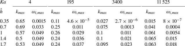
 $\omega _{i,max}$ of the growth rate peaks are reported in table 2. For
 $\hat {h}\leq 1$,
 $\omega _i$ gradually increases with
 $k$, up to the peak, then sharply decreases towards
 $k_m$. For
 $\hat {h}>1$,
 $\omega _i$ reaches the peak after a steep increase, and then it gently reaches
 $k_m$.
(a,c) Neutral curves for different values of the non-dimensional liquid-film thickness  $\hat {h}$, (b,d) dispersion relations normalised with
 $\max (\omega _i)$ and the cutoff frequency
 $k_c$ for
 $Re=30$ for (a,b) liquid zinc (
 $Ka=11\,525$) and (c,d) water
 $(Ka=3400)$.

(a,c) Neutral curve and (b,d) dispersion relations normalised with  $\max (\omega _i)$ and the cutoff frequency
 $k_c$, for
 $Re=30$ and different values of
 $\hat {h}$, for (a,b) liquid water–glycerol (
 $Ka=195$) solution and (c,d) corn oil (
 $Ka=4$).

Peak of growth rate  $\omega _{i,max}$ and the associated wavenumber
 $k_{max}$ for different liquids and
 $\hat {h}$ at
 $Re =30$.
As for the growth rate,  $\hat {h}$ also influences the neutral stability curves. For the four fluids, the instability region enlarges for large
 $\hat {h}$ and small
 $Ka$, with curves progressively gathering around the same wavenumbers for thick film conditions (
 $\hat {h}>1$), with the limit case of corn oil (
 $Ka=4$), where the neutral curves are almost superimposed. Similar behaviour is also visible in the dispersion relations. As
 $Ka$ decreases, the relative distance between the peaks’ positions for
 $\hat {h}> 0.35$ shrinks, with the limit case of corn oil (
 $Ka=4$) where the curves for
 $\hat {h}=0.4$ and
 $\hat {h}=1$ also change shapes, becoming similar to those for
 $\hat {h}>1$.
This highlights stabilising mechanisms given by the balance of inertia, viscous and gravitational forces without the effect of surface tension. As  $Ka$ decreases, the stabilising effects of the surface tension diminish compared with the viscous effects. Even when increasing
 $\hat {h}$, the instability region does not expand much. This suggests that neutral modes with
 $k=O(1)$ arise as an equilibrium of mostly viscous and gravitational forces, which is not linked to the velocity of the plate. Indeed, increasing
 $Re$ does not change the relative position of the neutral curves; it just brings this equilibrium point to larger
 $k$.
Figure 7 shows the evolution of (a) the  $\omega _i$ peak magnitude
 $\max (\omega _i)$ and (b) the wavenumber
 $k_{max}$ varying
 $\hat {h}$ for the different fluids. As
 $Ka$ decreases, the maximum growth rate increases. Corn oil (
 $Ka=4$) has the largest growth rates of all the
 $\hat {h}$ with its peaks overlapping for
 $\hat {h}\geq 1$.
Values of (a) the maximum growth rate  $\max (\omega _i)$ and (b) the associated wavenumber
 $k_m$ for different
 $\hat {h}$ and liquids at
 $Re=30$.

Interestingly, the peaks’ locations do not have a monotonic behaviour with  $\hat {h}$. For the corn oil (
 $Ka=4$), the peak position advances towards smaller wavelengths for
 $\hat {h}=0.7$, and then it goes to longer wavelengths for higher values of
 $\hat {h}$. As
 $Ka$ increases, the peak is located at smaller wavenumbers, and it moves to
 $\hat {h}=1.7$ passing through
 $\hat {h}=1$ for the water–glycerol (
 $Ka=195$) solution.
The liquid-film height  $\hat {h}$ and the Kapitza number also play a role in the phase speed of the unstable perturbations. Figure 8 shows how the phase speed
 $c_r$ as a function of the wavenumber
 $k$ and the liquid-film height
 $\hat {h}$ at
 $Re=30$ with a highlight on the neutral curve (continuous white line) and the positions of the maximum growth rate (white dashed line) for (a) liquid zinc (
 $Ka=11\,525$), (b) water (
 $Ka=3400$) and (c) corn oil (
 $Ka=4$). As we move along
 $k$ for a fixed
 $\hat {h}$, the phase speed varies first linearly (for small
 $\hat {h}$) and then nonlinearly (for large
 $\hat {h}$). This relation is quadratic for zinc (
 $Ka=11\,525$) and water, with the minimum at the same wavenumber of the maximum growth rate. In contrast, for the corn oil (
 $Ka=4$), after a steep variation for
 $k\rightarrow 0$, it becomes linear again with a minimum not coinciding with the peak of growth rate. As we move along
 $\hat {h}$ for a fixed
 $k$, the phase speed of long waves varies quadratically with
 $\hat {h}$, in accordance with the leading order approximation of the asymptotic expansion (B3) (
 $c_r = \hat {h}^2-1$). As we increase
 $k$, this approximation loses validity, with waves propagating slower. This relation tends to become linear as we move to shorter wavelengths. The slope of this relationship changes with
 $k$ and
 $Ka$, becoming almost insensitive to
 $k$, in the case of corn oil (
 $Ka=4$). High
 $Ka$, the most-unstable mode, travels slower than any other unstable mode.
Coloured surface showing the real part of the phase speed  $c_r$ as a function of the wavenumber
 $k$ and the flat liquid-film height
 $\hat {h}$ at
 $Re=30$ with the neutral curve (white continuous line) and maximum growth rate (white dashed line) for (a) liquid zinc (
 $Ka=11\,525$), (b) water (
 $Ka=3400$) and (c) corn oil (
 $Ka=4$).

5.2. Long-wave mechanism and energy balance of the unstable perturbation
In this subsection, we describe the mechanism behind the growth of unstable perturbations using momentum and vorticity arguments. Moreover, we investigate how the perturbation's energy is extracted and stored depending on the values of the non-dimensional groups and the liquid-film height, highlighting the role of viscous terms. In the falling-liquid-film case, Kelly et al. (Reference Kelly, Goussis, Lin and Hsu1989), with the energy-based approach, and Smith (Reference Smith1990), with asymptotic expansions, showed that the long-wave instability is fed by a streamwise flow field resulting from the base state's shear stress deficiency at the free-surface.
5.2.1. Long-wave instability mechanism
Considering the harmonic disturbance  $\tilde {h}$ over a flat interface
 $\bar {h}$ (see § 4.1), the shear stress at the perturbed interface is given by a base state and a perturbation contribution. Expanding
 $D \hat {u}$ around the base state thickness
 $\bar {h}$, we obtain, at first order,
 \begin{equation} D \hat{u}(\hat{h}) = D\bar{u}(\bar{h}) + D\tilde{u}(\bar{h}) + D^2\bar{u}(\bar{h})\tilde{h} =0. \end{equation}
Since the base state is shear-free at the interface ( $D\bar {u}(\bar {h})=0$) and knowing that
 $D^2\bar {u}(\bar {h})=-1$, (5.3) reduces to
 \begin{equation} D\tilde{u}(\bar{h}) - \tilde{h}=0. \end{equation}
The equilibrium of forces implies that the disturbance has to generate a positive shear stress  $D\tilde {u}(\bar {h})$ to compensate for
 $\tilde {h}$. To analyse this mechanism, we considered a reference frame moving at the substrate velocity
 $U_p$ (
 $\hat {u}=-1$), and we expand the streamwise velocity amplitude
 $\acute {u}$ in a power series of
 $k$ assuming long-wave conditions (4.1) (Smith Reference Smith1990). The solution at
 $O(1)$ of (4.4) with boundary conditions (4.5) is given by a linear velocity amplitude
 $\acute {u}_{m0}(\hat {y})$ and a positive phase speed
 $c_{m0}$:
 \begin{equation} \acute{u}_{m0}(\hat{y}) = \hat{y} + 1, \quad c_{m0} = \bar{h}^2. \end{equation}
The behaviour of  $c_{m0}$ is solely determined by gravity. The thicker the base state, the more gravity is important, and the more the wave travels faster downwards along the
 $\hat {x}$ direction.
Figure 9(a) shows the flow field at leading order as a consequence of a harmonic displacement of the interface (red line). Since the flow field is in phase with the liquid-film displacement, the streamwise velocity is maximum at the peak and minimum at the trough. Considering a control volume in the range  $\theta \in [0,{\rm \pi} /2]$, enclosed between a peak and a node at the interface, this has a positive net flow rate. The velocity field pushes liquid to the right at the crest, with a zero flow rate at the node. In accordance with the continuity equation, this implies a positive displacement of the film interface to accommodate this accumulation of mass, leading to a travelling wave in the positive
 $\hat {x}$ direction. The solution of (4.6a) gives the normal velocity at
 $O(k)$:
 \begin{equation} v_{1} ={-}i\hat{y}^2/2. \end{equation}
The link between the phase speed and the flow rate is given by the kinematic boundary condition at the interface (4.7b):
 \begin{equation} c_{m0} - \bar{u}_m(\hat{h}) = v_{1} =\int_{0}^{\hat{h}}u_{m0}-1\,{\rm d}\hat{y} = \hat{h}^2/2. \end{equation}
Magnitude (greyscale) and vector field (arrows) of the perturbation's velocity field (a) at leading order and (b) at first order in the wavenumber  $k$.

This initiating mechanism affects the development of the flow field at  $O(k)$ through two inertial stresses in (4.6b):
 \begin{equation} -{\rm i}Re(u_{m0}(\hat{y}) -1)(\bar{u}_m(\hat{y}) - c_{m0} - 1) \quad \text{and} \quad Re\, v_{1}(\hat{y})D\bar{u}_m(\hat{y}). \end{equation}
The first term corresponds to the advection of the reduced leading-order solution by the base state velocity with respect to the reduced leading order wave speed. The second term corresponds to the advection of the base state velocity by the first-order wall-normal velocity  $v_1$. Since the phase speed
 $c_{m0}$ is larger than any values in
 $\bar {u}_m(\hat {y})$, and being
 $D\bar {u}_m(\hat {y})=-\hat {y} + \hat {h}$ positive for all
 $\hat {y}\in [0,\hat {h}]$, these two terms are both negative. This leads to a destabilising flow field given by the solution of the first-order equations (4.6) with boundary conditions (4.7):
 \begin{equation} u_{m1}(\hat{y}) = \frac{Re}{24} {\rm i} (8\hat{h}^4\hat{y} - 4\hat{h}^2\hat{y}^3 + 12\hat{h}\hat{y} + \hat{h}\hat{y}^4 - 4\hat{y}^3). \end{equation}
Figure 9(b) shows the flow field calculated with (5.9). Since the velocity amplitude  $u_{m1}(\hat {y})$ is imaginary and positive, the flow has a phase shift of
 ${\rm \pi} /2$ with respect to the wave displacement. Consequently, the velocity pushes fluid from the troughs to the peaks, sustaining the growth of the perturbation. This renders a growth mechanism based on the extraction of energy contained in the leading-order solution, which, in turn, extracts energy from the base state through the work done by the shear stress at the interface.
5.2.2. Vorticity perturbation at the free surface and in the bulk
In the previous subsection, we studied the general structure of the instability mechanism. The first-order solution in  $k$, fed by leading-order inertial stresses, generates a destabilising flow from the troughs to the peaks due to a
 ${\rm \pi} /2$ phase shift to the free-surface displacement. In this section, we go into more detail, analysing how the phase shift and the magnitude of the perturbation change with the wavenumber and the flat liquid-film height. To this end, we look at the growth of the perturbation in terms of the vorticity field. The perturbation's shear stress correction in (5.4) can be seen as a source of vorticity at the free surface
 $\omega _{FS}$. We consider a reference frame moving with the wave speed
 $c_r$, i.e.
 $\theta =k(\hat {x}-c_r\hat {t})$, and we assume a sinusoidal displacement of the free surface:
 \begin{equation} \tilde{h} = \sin{(\theta)}, \end{equation}
with  $\theta =0$ at 0, this implies through (4.12a), that
 \begin{equation} \eta_r = 0,\quad \eta_i ={-}1. \end{equation}
By means of the kinematic boundary condition (2.22b), we scale the eigenfunction such that
 \begin{equation} \phi_r(\hat{h}) = c_i, \quad \phi_i(\hat{h}) ={-}\hat{c}. \end{equation}
The shear stress condition (2.22d) imposes that
 \begin{equation} D^2\phi_r(\hat{h}) ={-}k^2 c_i, \quad D^2\phi_i(\hat{h}) ={-}2 + k^2\hat{c}. \end{equation}
By replacing these expressions in (4.10d), we obtain the vorticity at the free surface:
 \begin{equation} \omega_{FS} = \gamma \sin{(\theta - \xi)}, \end{equation}
with the amplitude  $\gamma$ and the phase shift
 $\xi$ given by
 \begin{equation} \gamma = 2\sqrt{(1-k^2\hat{c})^2 + (k^2c_i)^2]}, \quad \xi = \arctan{(k^2c_i/(1-k^2\hat{c})}. \end{equation}
Depending on  $\xi$,
 $\omega _{FS}$ stabilises (
 $\xi <0$) or destabilises (
 $\xi >0$) the free-surface displacement (Kelly et al. Reference Kelly, Goussis, Lin and Hsu1989).
Figure 10 shows (a,d) the growth rate  $\omega _i$, (b,e) the amplitude
 $\gamma$ and (c,f) the phase shift
 $\xi$ of the free-surface vorticity as a function of the wavenumber
 $k$ and the liquid-film thickness
 $\hat {h}$ at
 $Re=30$, with the neutral curve (continuous red line) and the maximum growth rate (dashed red line) for (a–c) the corn oil (
 $Ka=4$) and (d–f) the liquid zinc (
 $Ka=11\,525$). For a fixed
 $k$,
 $\omega _i$ gently grows with
 $\hat {h}$ driven by a vorticity with a large amplitude and a very small positive phase shift. For
 $\hat {h}=1$,
 $\omega _i$ grows more sharply, accompanied by an increase in the phase shift and a decrease in the vorticity amplitude. In the corn oil (
 $Ka=4$) case, the growth rate and the phase shift reach a plateau for large
 $\hat {h}$, in line with the saturating mechanism introduced in § 5.1. The phase shift
 $\xi$ peaks at higher wavenumbers than the growth rate
 $\omega _i$. The decay of the vorticity amplitude
 $\gamma$ with
 $k$ compensates for the destabilising effect of larger phase shifts, decreasing the growth rate. This suggests that the instability mechanism is also driven by the vorticity in the bulk, thus confirming the results in the previous subsections.
(a,d) Growth rate, (b,e) free-surface vorticity amplitude and (c,f) phase shift as a function of  $k$ and
 $\hat {h}$ with the neutral curve (continuous red line) and the positions of maximum growth rates (red dashed line) for
 $Re=30$, considering (a–c) corn oil (
 $Ka=4$) and (d–f) zinc (
 $Ka=11\,525$).

To investigate this behaviour, we analysed the vorticity perturbation  $\tilde {\omega }(\theta,\hat {y})=\partial _{\hat {x}}\tilde {v} - \partial _{\hat {y}}\tilde {u}$ within the liquid film. The vorticity equation is obtained by taking the curl of the momentum equations (2.14b) and (2.14c), considering the continuity equations (2.14a) and the base state (2.11), which leads to
 \begin{equation} \partial_{\hat{t}}\tilde{\omega} + \bar{u}\partial_{\hat{x}}\tilde{\omega} - \tilde{v}D^2\bar{u} = \frac{1}{Re}(\partial_{\hat{x}\hat{x}}\tilde{\omega} + D^2\tilde{\omega}). \end{equation}
Considering the reference frame moving with the wave speed  $c_r$ and knowing that
 $D^2\bar {u}=-1$, we obtain
 \begin{equation} k(\bar{u}-c_r)\partial_{\theta}\tilde{\omega} + \tilde{v} = \frac{1}{Re}(k^2\partial_{\theta\theta}\tilde{\omega} + D^2\tilde{\omega}). \end{equation}
On the left-hand side, the first term corresponds to the advection relative to the wave velocity, and the second term corresponds to the vorticity perturbation's advection of the base state. The term on the right-hand side corresponds to the viscous diffusion of vorticity. Inserting a normal mode solution for the vorticity with  $k\in \mathbb {R}$ and
 $c = c_r + {\rm i}c_i$,
 \begin{equation} \tilde{\omega} = \acute{\omega}(\hat{y})\exp({\rm i}k(\hat{x} - c\hat{t})) = \acute{\omega}(\hat{y})\exp(kc_i\hat{t})\exp({\rm i}\theta), \end{equation}
and for the wall-normal velocity given by (4.1) in (5.17) leads to the expression for the free-surface amplitude  $\acute {v}(\hat {y})$,
 \begin{equation} \acute{v}(\hat{y}) = {\rm i}k(c_r - \bar{u}(\hat{y}))\acute{\omega}(\hat{y}) + \frac{1}{Re}({-}k^2 + D^2)\acute{\omega}(\hat{y}). \end{equation}
Note that for  $Re\gg 1$, the relation reduces at leading order in
 $k$ to
 \begin{equation} \acute{v}(\hat{y}) \approx {\rm i}k(c_r - \bar{u}(\hat{y}))\acute{\omega}(\hat{y}) , \end{equation}
which corresponds to neglecting viscous effects.
Approximating  $c_r$ with the long-wave asymptotic solution at
 $O(1)$ in (B3), the term
 $c_r -\bar {u}$ is always positive
 $\forall \hat {y}\in [0,\hat {h}]$, implying that the vertical velocity amplitude changes linearly with the vorticity amplitude with a phase shift of
 ${\rm \pi} /2$ along
 $\theta$.
Figure 11 shows the perturbation (a, b, c, g, h and i) vorticity and (d, e, f, j, k and l) normal velocity fields at (a–f)  $\hat {h}=0.7$ and (g–l)
 $\hat {h}=1.7$ for the corn oil (
 $Ka=4$) with
 $k=0.5$ (a, d, g and j), 0.93 (b, e, h and k) and 1.2 (c, f, i and l) with the maximum (red square) and minimum (red triangle) of vorticity at the interface with
 $Re=30$. For
 $k=0.5$, the vorticity contours deform towards the left, advected by the flow. Since the advection velocity strengthens, this tilting effect is more intense for large
 $\hat {h}$. This structure recalls the capillary separation eddy in a falling liquid film of finite amplitude in the capillary flow region (Dietze, Al-Sibai & Kneer Reference Dietze, Al-Sibai and Kneer2009). The induced normal velocity field changes sign at the peak of vorticity along
 $\theta$, leading to a positive (negative) net vertical flow rate under the crests (trough), which fosters the growth of the perturbation.
Perturbation (a, b, c, g, h and i) vorticity and (d, e, f, j, k and l) normal velocity fields at (a–f)  $\hat {h}=0.7$ and (g–l)
 $\hat {h}=1.7$ for the corn oil (
 $Ka=4$) with
 $k=0.5$ (a, d, g and j), 0.93 (b, e, h and k) and 1.2 (c, f, i and l) with the maximum (red square) and minimum (red triangle) of vorticity at the interface with
 $Re=30$.

As the wavenumber increases, the vorticity lines bend towards the right near the substrate. This curvature stabilises the perturbation, enlarging the negative (positive) normal velocity area under the peak (trough). At the same time, the vorticity tends to concentrate near the free surface, approaching its maximum value at the interface and forming a boundary layer region with strong shear stresses. Despite the differences in the vorticities and normal velocities’ distributions, the stability mechanism at  $\hat {h}=0.7$ and
 $\hat {h}=1.7$ for the corn oil (
 $Ka=4$) is very similar. As we have seen, the neutral curves and the dispersion relations (figure 6), the vorticity at the free surface (figure 10) and the order of magnitude of the vorticity in bulk are almost the same for the two conditions. This means that for small
 $Ka$, the instability growth is mainly driven by the vorticity at the free surface and in its proximity.
Things change as we move to larger  $Ka$. Figure 12 shows the perturbation (a, b, c, g, h and i) vorticity and (d, e, f, j, k and l) normal velocity fields at (a–f)
 $\hat {h}=0.7$ and (g–l)
 $\hat {h}=1.7$ for the liquid zinc (
 $Ka=11\,525$) with
 $k$ equal to (a,d) 0.002, (g,j) 0.003, (b,e) 0.047, (c,f) 0.051, (h,k) 0.077 and (i,l) 0.15 with the maximum (red square) and minimum (red triangle) of vorticity at the interface at
 $Re=30$. For
 $\hat {h}=0.7$, the advection has a very small effect on the vorticity contour's curvature. The viscous effects almost completely dominate the vorticity distribution. As we have seen in figure 10, for
 $\hat {h}=0.7$, the instability grows mostly due to the vorticity magnitude rather than the phase shift, which is almost zero.
Perturbation (a, b, c, g, h and i) vorticity and (d, e, f, j, k and l) normal velocity fields at (a–f)  $\hat {h}=0.7$ and (g–l)
 $\hat {h}=1.7$ for the liquid zinc (
 $Ka=11\,525$) with
 $k$ equal to (a,d) 0.002, (g,j) 0.003, (b,e) 0.047, (c,f) 0.051, (h,k) 0.077 and (i,l) 0.15 with the maximum (red square) and minimum (red triangle) of vorticity at the interface at
 $Re=30$.

For  $\hat {h}=1.7$, the vorticity lines tilt in the advection direction as we increase the wavenumber. Moreover, for
 $k =0.15$, a region of intense vorticity is created near the substrate, destabilising the flow, increasing the net flow rate under the crests, and creating a boundary layer near the substrate in addition to that near the free surface.
This region is the product of the streamwise pressure gradient induced by the surface tension. The normal vorticity flux at the substrate, also known as vorticity source strength (Lighthill Reference Lighthill1963), is given by(Morton Reference Morton1984)
 \begin{equation} -\partial_{\hat{y}}\omega = \partial_{\hat{x}}\tilde{p} - 1, \end{equation}
where the right-hand side represents the rate of vorticity production per unit area and comprises the perturbation's streamwise pressure gradient and the gravitational effect. Positive vorticity is generated when the streamwise pressure gradient outweighs the gravitational effect.
For small  $k$, the pressure is constant a long
 $\hat {y}$, with the most-sensitive zone to the surface tension close to the substrate. As we have shown in Appendix B.2, for high
 $Ka$, the surface tension influences the first-order solution for small
 $k$. The first-order streamwise velocity amplitude, derived by differentiating the stream function (B5) with respect to the wall-normal coordinate, is given by
 \begin{equation} \acute{u}_1 = D \varphi_1^{{\star}}(\hat{y}) = \frac{{\rm i} \hat{y}^2}{12}(\hat{h}\,Re\,\hat{y}^2 - 4\hat{h}^2Re\hat{y} + 12k^2\,Ca ). \end{equation}
Assuming  $\hat {h}=O(1)$, the surface tension term is dominant for small
 $\hat {y}$ i.e. near the substrate.
Moreover, the surface tension also increases the vorticity near the free surface (figure 12e and f). The normal vorticity flux at the interface is given by (Dietze et al. Reference Dietze, Al-Sibai and Kneer2009; Wu Reference Wu1995)
 \begin{equation} -\partial_{\hat{n}}\tilde{\omega} = \frac{\partial_{\hat{x}}\tilde{p}}{\sqrt{1 + (\partial_{\hat{x}}\tilde{h})^2}}, \end{equation}
where  $\hat {n}$ is the non-dimensional normal vector to the interface pointing toward the liquid. As for the substrate flux, it depends on the streamwise pressure gradient. At a peak (trough) location, the pressure gradient in the streamwise direction is negative (positive), so the film produces positive (negative) vorticity at the free surface.
The mechanism leading to the formation of this boundary layer zone is as follows: the pressure imposed by the surface tension pushes fluid down (up) at the crests (troughs), which, via the continuity equation, produces a positive (negative) streamwise flow near the substrate. The movement of the substrate increases the shear effects compared with the falling film case, leading to more intense vorticity regions.
These outcomes highlight the importance of  $Ka$, even for long-wave perturbation (small
 $k$). This means that surface tension is crucial for stabilising short waves and storing perturbation energy and for the early development of instability and vorticity distribution in liquid film. Moreover, we reveal two mechanisms of instability involving viscous stresses associated with the boundary layer at the free surface for the corn oil (
 $Ka=4$) and the boundary layer at the substrate for the zinc (
 $Ka=11\,525$).
5.2.3. Energy balance of the perturbation
We have analysed the early stages of the long-wave instability mechanism and how the vorticity at the free surface and in bulk fosters the growth of unstable perturbations. Here, we study the terms forming the kinetic energy balance (4.8a) of an unstable perturbation, as presented in § 4.2.
The vorticity near the substrate also affects the dissipation terms defined in (4.8f) and (4.9). Figure 13 shows the elongational ( ${\rm DISSI}_1$ green dashed-dotted line with circles and
 ${\rm DISSI}_3$ orange dashed line with triangles) and shear (
 ${\rm DISSI}_2$ blue dashed line with squares) stresses contributing to the total dissipative viscous effects (
 ${\rm DISSI}_{tot}$ red continuous line) as a function of
 $k$ at
 $\hat {h}=1.7$ and
 $Re=30$ for (a) corn oil (
 $Ka=4$) and (b) liquid zinc (
 $Ka=11\,525$). Here
 ${\rm DISSI}_1$ is equal to
 ${\rm DISSI}_3$ due to the continuity equation. For small
 $k$,
 ${\rm DISSI}_2$, which is a function of the strain rate
 $\upsilon$, dominates the dissipative effects, with
 ${\rm DISSI}_1$ and
 ${\rm DISSI}_2$ slowly increasing with
 $k$. For larger
 $k$,
 ${\rm DISSI}_2$ decreases in magnitude. At
 $Ka=4$ (corn oil), it decreases monotonically with
 $k$, whereas for
 $Ka=11\,525$ (zinc), it reaches a minimum and increases again towards the cutoff wavenumber. This is due to the creation of a boundary layer near the substrate. Near the boundary, the strain rate
 $\upsilon$ is equal to the vorticity, and they are both generated with the same boundary flux densities (Morton Reference Morton1984). In addition to the boundary, the bulk is also a source of strain rate. The equation governing the strain rate is given by
 \begin{equation} \partial_{\hat{t}}\upsilon ={-}2 \partial_{\hat{x}\hat{y}}\tilde{p} + \frac{1}{Re}(\partial_{\hat{x}\hat{x}}\upsilon + \partial_{\hat{y}\hat{y}}\upsilon). \end{equation}
When the surface tension induces a pressure gradient in the liquid film, the bulk also generates a strain rate, feeding  ${\rm DISSI}_2$.
Distribution of the extensional stresses  ${\rm DISSI}_1$ and
 ${\rm DISSI}_3$ and shear stress
 ${\rm DISSI}2$, with
 $\hat {h}=1.7$ and
 $Re=30$ for (a) the corn oil (
 $Ka=4$) and (b) the liquid zinc (
 $Ka=11\,525$).

5.3. Absolute/convective (AC) threshold
The previous subsections focused on the instability mechanism using long-wave expansions, vorticity and energy arguments. In this subsection, we further extend our analysis of unstable perturbations of Pino, Mendez & Scheid (Reference Pino, Mendez and Scheid2024), calculating the AC threshold in the  $\hat {h}$–
 $Re$ and
 $c_r$–
 $Re$ parameter spaces with the LLD solution
 $\mathop{h}\limits^{\circ}$, the real part of the wavenumber
 $k_r$ (red empty triangles) and the non-dimensional capillary length
 $\hat {\ell }_{c}$ defined in (2.9) (blue continuous line with empty squares), for the liquids in table 1. Moreover, we calculate the threshold also in the
 $Ka$–
 $Re$ space for the Derjaguin solution (
 $\hat {h}=1$). The region of absolute instability is depicted as a shaded area bounded by the AC threshold simulated points (continuous black line with black circles).
In the literature on falling films, Brevdo et al. (Reference Brevdo, Laure, Dias and Bridges1999) showed that a flat liquid film over a vertical substrate is always convectively unstable due to gravitational effects. In the case of an inclined substrate, the hydrostatic effects compensate for the gravity, leading to regions of absolute instability (Brun et al. Reference Brun, Damiano, Rieu, Balestra and Gallaire2015; Scheid et al. Reference Scheid, Kofman and Rohlfs2016). Similarly, the leading actors in the moving substrate case are gravity, inertia, viscosity and surface tension. For certain parameters, these compensate for each other, leading to regions of absolute instability.
5.3.1. AC threshold in the  $Ka$–$Re$ space with $\hat {h}=1$


Figure 14 shows the AC threshold for the Derjaguin solution ( $\hat {h}=1$) in (a) the
 $Ka$–
 $Re$ parameter space, with the trend line
 $Ka=0.15Re^{1.8}$ (red dashed line) and in (b) the
 $c_r$–
 $Re$ space. For
 $Ka<30$, the threshold has a minimum of
 $Ka=17$ at
 $Re=3$ and a maximum of
 $Ka=25$ at
 $Re=0.4$. For
 $Ka>30$ and
 $Re\gtrsim 10$, it gets to an asymptote, which goes as
 $Ka\sim Re ^{1.8}$ or in terms of capillary number as
 $Ca^{-1}\sim Re ^{1.5}$. These results show that for fluids with
 $Ka<17$, the Derjaguin solution is always convectively unstable regardless of the Reynolds number.
AC threshold (black dotted line) of the Derjaguin flat film solution ( $\hat {h}=1$) in (a) the
 $Ka$–
 $Re$ space with the trend line
 $Ka=0.15Re^{1.8}$ (red dashed line) and in (b)
 $c_r$–
 $Re$ space with the associated real wavenumber
 $k_r$ (red triangles) and non-dimensional capillary wavenumber
 $k_{\ell _{c}}$ (continuous blue line with blue squares).

The neutral perturbations ( $\omega _i=0$) associated with the AC threshold have a negative phase speed for every
 $Re$. These travel faster than the substrate speed (
 $|c_r|>|U_p|$) for
 $Re\gtrsim 5.5$. The phase speed has a maximum at
 $Re=0.1$ and an asymptote at
 $c_r~2.7$ for
 $Re>300$. The real wavenumber
 $k_r$ of the neutral perturbations has a maximum at
 $k_r\approx 0.8$ in the range
 $100< Re<200$. For
 $Re>300$,
 $k_r$ exceeds
 $\hat {\ell }_{c}$, highlighting how, at these wavelengths, surface tension starts to dominate over gravity.
5.3.2. AC threshold in the $\hat {h}$–$Re$ space for different $Ka$


Moving to the AC threshold for the liquids in table 1, from figures 15–16 show the window of absolute instability in (a) the  $\hat {h}$–
 $Re$ space bounded by a lower and an upper threshold (black dots) and in (b) the
 $c_r$–
 $Re$ space, with the real wavenumber
 $k_r$ of the upper (red empty triangular markers) and lower thresholds (red empty circular markers). We also show a second AC upper threshold (green empty markers) and the LLD solution
 $\mathop{h}\limits^{\circ}$ (dash-dotted orange line) for the water–glycerol (
 $Ka=195$) solution and corn oil (
 $Ka=4$). The absolute region's extrema and the upper threshold inflection points are reported in table 3.
Upper and lower branches of the absolute instability region (black dots) in (a,c) the  $\hat {h}$–
 $Re$ and (b,d)
 $c_r$–
 $Re$ spaces with the associated wavenumber
 $k_r$ for the lower (circles) and upper (triangles) thresholds and the curve
 $k_{\ell _c}$ (dashed blue line) for (a,b) liquid zinc (
 $Ka=11\,525$) and (c,d) water (
 $Ka=3400$).

Upper and lower branches of the absolute instability region (black dots) in (a,c) the  $\hat {h}$–
 $Re$ space with the second branch of the upper threshold (green empty triangles) and the LLD solution (orange dash- dotted line) and in (b,d) the
 $c_r$–
 $Re$ space with the associated wavenumber
 $k_r$ for the lower (circles) and upper (triangles) thresholds and the curve
 $k_{\ell _c}$ (dashed blue line) for (a,b) water–glycerol (
 $Ka=195$) and (c,d) corn oil (
 $Ka=4$).

Maximum and minimum of the absolute instability windows in the  $\hat {h}$–
 $Re$ space for different liquids.

For the four liquids, the lower threshold stems from  $\hat {h}=1$ as
 $Re\rightarrow 0$ and develops mainly in the thin film domain, with a minimum at intermediate
 $Re$ values. The threshold extends into the thick film domain, with a plateau at
 $\hat {h}\approx 1.4$ for water–glycerol (
 $Ka=195$) and corn oil (
 $Ka=4$). The lower threshold of the corn oil extends solely into the thick film, with thin film base states (
 $\hat {h}<1$) always convectively unstable. In the
 $c_r$–
 $Re$ space, the neutral waves associated with the lower threshold travel upward against gravity (
 $c_r<0$). The associated wavenumber
 $k_r$ monotonically increases with
 $Re$. Here
 $k_r$ overtakes
 $k_{\ell _{c}}$ for the liquid zinc (
 $Ka=11\,525$) and water, showing that the surface tension prevails over gravity for large
 $Re$. Due to surface tension effects, which support the entrainment action against gravity for intermediate
 $Re$, the minimum of the lower threshold
 $\hat {h}_{min}$ decreases with
 $Ka$, following the relations:
 \begin{equation} Re_{min} = 1.5496Ka^{0.4677}, \quad \hat{h}_{min} ={-} 0.0022Re_{min} + 0.9403, \end{equation}
where  $Re_{min}$ is the
 $Re$ associated to
 $\hat {h}_{min}$.
The upper thresholds stem from  $\hat {h}=1$ and extend into the thick film domain (
 $\hat {h}>1$) with a maximum of
 $\hat {h}\approx 1.65$ at
 $Re\approx 10$ and a plateau at
 $\hat {h}\approx 1.5$ for
 $Re>100$. In the
 $c_r$–
 $Re$ space, the neutral waves, associated with the upper threshold, travel downwards (
 $c_r>0$) with a maximum at
 $Re\approx 1$ for corn oil (
 $Ka=4$) and
 $Re\approx 100$ for the other liquids. As for the lower branch, based on the liquid's properties, we define the value of
 $\hat {h}_{max}$ and the associated
 $Re$ (
 $Re_{max}$) as a function of
 $Ka$ via the relations
 \begin{equation} Re_{max} = 1.9372Ka^{0.2732}, \quad \hat{h}_{max} ={-} 0.0008Re_{max} + 1.6663. \end{equation}
Considering the operational range of the hot-dip galvanising process, using liquid zinc with  $Re\in [437,2273]$ and
 $\hat {h}<0.2$, the flat liquid film is always convectively unstable.
In addition to the saddle point defining the upper branch, we found other valid saddle points for water–glycerol ( $Ka=195$). Figure 17 shows two saddle points (red circle and red square) (a) in the complex wavenumber space
 $k_r$–
 $k_i$ with the
 $\omega _i$ colour map and (b) in the complex frequency space
 $\omega _r$–
 $\omega _i$ with the spatial branches along the real
 $k$ axis with
 $k_i=0$ for water–glycerol (
 $Ka=195$) at
 $\hat {h}=1.48$ and
 $Re=100$. The two saddle points satisfy the collision criterion since an odd number of temporal branches surmount them. Based on the second saddle point (red square), which appears around
 $Re\approx 40$, we traced another AC threshold (green empty triangles in figure 16a). Interestingly, this threshold is always below the first and approaches the lower branch for larger
 $Re$, closing the window of absolute instability. This is also visible in the
 $c_r$–
 $Re$ space (green triangles in figure 16b), where the phase speed of the two branches converges. Moreover, the wavenumber increases with
 $Re$ reaching 0.5 for
 $Re=3000$.
Position of two saddle points (red circle and red square) in (a) the  $k_r$–
 $k_i$ space with the
 $\omega _i$ colour plot and in (b) the
 $\omega _r$–
 $\omega _i$ space with the temporal branches along the real wavenumber axis with
 $k_i=0$ (continuous coloured lines) for water–glycerol (
 $Ka=195$) with
 $\hat {h}=1.48$ and
 $Re=100$.

For  $Re=3000$, we discovered a collection of saddle points near the imaginary wavenumbers’ axis. Figure 18 shows the position of six saddle points with (a,c) red markers in the
 $k_r$–
 $k_i$ space with the
 $\omega _i$ colour map and with (b,d) coloured markers in the
 $\omega _r$–
 $\omega _i$ space and the temporal branches along the real wavenumber axis (coloured lines) with
 $\hat {h}=1.41$ and
 $Re=3000$ for (a,b) water–glycerol (
 $Ka=195$) and (c,d)
 $Ka=0$. The first saddle point is used to construct the AC threshold described previously. For plotting convenience, we do not show the saddle point of the second upper branch because it is at a much larger real wavenumber. Only the first four of the six saddle points respect the collision criterion, with the first being the last to have a negative growth rate as we increase
 $\hat {h}$. Since the AC associated with this point represents the upper bound for the region of absolute stability, we did not investigate the AC for the other saddle points. The location of these saddle points is invariant with
 $Ka$ since their positions are the same for the case with water–glycerol and
 $Ka=0$. This implies that this part of the AC upper branch is not affected by the surface tension and is solely given by a balance of gravity and inertia.
Multiple saddle points in (a,c) the complex wavenumber space  $k_r$–
 $k_i$ (numbered red markers) and (b,d) in the complex frequency domain
 $\omega _r$–
 $\omega _i$ (empty coloured markers) with the temporal branches along the real wavenumber axis (coloured continuous line) at
 $Re=3000$ and
 $\hat {h}=1.41$ for (a,b) water–glycerol (
 $Ka=195$) and (c,d)
 $Ka=0$.

The LLD solution  $\mathop{h}\limits^{\circ}$ (defined in (2.10)) is always convectively unstable for zinc (
 $Ka=11\,525$), water (
 $Ka=3400$) and water-glycerol (
 $Ka=195$). For convenience, we did not report this curve for liquid zinc and water because it was much smaller
 $\hat {h}$ compared with the window of absolute instability. For corn oil (
 $Ka=4$),
 $\mathop{h}\limits^{\circ}$ crosses the area of absolute instability in the range
 $100< Re<500$. However, since this intersects the lower branch at a
 $Re\approx 300$, it is unrealistic to see it in an experiment. In addition, given that the wavenumber of the lower branch is tiny, this would require a very long domain for substrate velocities in the range
 $U_p\in [0.1$–
 $1]$ (m s
 $^{-1}$).
We rescale the upper and lower AC thresholds in the  $\hat {h}$–
 $Re$ space with (
 $\hat {h}_{max},Re_{max}$) and (
 $\hat {h}_{min},Re_{min}$), respectively, for liquid zinc (
 $Ka=11\,525$), water (
 $Ka=3400$) and water–glycerol (
 $Ka=195$). Figure 19 shows the scaled (a,b) upper and (c,d) lower thresholds in (a,c) the
 $\hat {h}$–
 $Re$ and (c,d) the
 $\breve {h}$–
 $Re$ spaces for the liquid zinc (
 $Ka=11\,525$) (red circle), water (
 $Ka=3400$) (blue squares) and water–glycerol (
 $Ka=195$) (green triangles), where
 $\breve {h}$ is the non-dimensional film thickness based on the viscous length
 $\ell _{\nu }$ defined in (2.4). The curve matches perfectly apart from the lower bound in the
 $\hat {h}$–
 $Re$ space at small and large
 $Re$. Moreover, we found a simple approximation to the lower AC threshold. Figure 19(d) shows a trend line (black loosely dashed line) for the lower branch, given by
 \begin{equation} \breve{h}/\breve{h}_{min}=(Re/Re_{min})^{4/9}. \end{equation}
This approximation enables the construction of the absolute instability window for any fluid within the range  $Ka\in [195,11\,525]$ without the need for further simulations.
Scaled absolute instability window for liquid zinc ( $Ka=11\,525$; red circles), water (
 $Ka=3400$; blue squares) and water-glycerol (
 $Ka=195$; green triangles), with the (a,b) upper and (c,d) lower AC thresholds rescaled with their values at the maximum and the minimum in (a,c) the
 $\hat {h}$–
 $Re$ and (b,d) the
 $\acute {h}$–
 $Re$ space with the trend line
 $\breve {h}/\breve {h}_{min}=(Re/Re_{min})^{4/9}$ (dashed black line).

6. Conclusion and perspectives
This study investigated the linear stability of a vertical liquid film over a substrate moving against gravity for four liquids with  $Ka$ numbers ranging from 4 to 11 525. We have identified the region of unstable perturbations by using long-wave asymptotic analysis and numerical solutions to the Orr–Sommerfeld eigenvalue problem. The instability mechanism has been described for the unstable solutions via momentum, vorticity and energy-based arguments, and the threshold between absolute and convective instability has been traced.
The neutral curves, growth rates and phase speed converge around the same values for  $\hat {h}\gtrsim 0.7$, highlighting a stabilising mechanism where viscous effects balance gravitational effects with minimal influence from surface tension.
For thin films, the instability is driven by the amplitude of the vorticity with a minimal phase shift. For thick films, the amplitude decreases and the phase shift increases, with a peak shifted at larger  $k$. The surface tension strongly affects this mechanism, simultaneously stabilising and destabilising the film, especially for
 $Ka=11\,525$. For long waves, this curves the vorticity lines near the substrate, reducing the flow under the crests. For short waves, this enhances vorticity production at the free surface and creates a region of intense vorticity near the substrate.
Intense Reynolds stresses accompany areas of intense vorticity. At the same time, the dissipative terms also grow in magnitude, leading to two instability mechanisms for small and large  $Ka$. For
 $Ka=11\,525$, surface tension induces a larger vorticity production at the free surface and at the wall, resulting in significant Reynolds stresses and intense dissipative effects. In addition, the contribution to the viscous terms also increases. For
 $Ka=4$ (corn oil), shear effects mainly influence the viscous term. The shear effects diminish for
 $Ka=11\,525$ (zinc), and the extensional term becomes more important.
In terms of AC instability threshold, for  $Ka<17$ the LLD solution is always convectively unstable for any
 $Re$ whereas for
 $Re\gtrsim 10$, the threshold follows an asymptote given by
 $Ka\approx 0.15\ Re ^{1.8}$. In the
 $\hat {h}$–
 $Re$ space, a window of absolute instability arises between the thin and thick film conditions. This window develops solely in the thick film region for
 $Ka=4$ (corn oil). Moreover, a bifurcation point is also present at
 $Re\approx 40$, where two solution branches exist, one independent of
 $Ka$. Rescaling the lower (upper) branch of the absolute instability window with its minimum (maximum), the curves for
 $Ka>4$ converge in the
 $\hat {h}$–
 $Re$ space. A relation linking the value of
 $Re$ at the minimum of this curve to the lower bound was also provided.
These findings provide crucial insights into the stability of the liquid film in dip-coating processes. Our analysis helps validate reduced-order models by comparing their predicted growth rates and neutral curves. By leveraging the numerical and analytical solutions of the Orr–Sommerfeld problem, we can develop optimal control strategies for external actuators to stabilise linearly unstable perturbations.
Future investigations could build on our findings by examining whether perturbations exhibit remnant behaviour, with waves propagating in both directions, as well as exploring transient growth mechanisms or transverse modulation due to nonlinear effects in three dimensions. Understanding instability mechanisms without external influences such as magnetic fields or airflow lays a solid foundation for more detailed studies incorporating these factors. Furthermore, direct numerical simulations could assess the accuracy of the AC threshold and uncover additional unstable saddle points in complex frequency space driven by nonlinear effects.
Funding
F.P. is supported by an F.R.S.-FNRS FRIA grant, and his PhD research project is funded by Arcelor-Mittal. B.S. is Research Director at F.R.S.-FNRS.
Declaration of interest
The authors report no conflict of interest.
Appendix A. Pseudocode for the search of the AC threshold
The pseudocode (Algorithm 1) reports the main steps of the AC threshold search. First, we define the liquid properties and the Kapitza number. Then we select a range of Reynolds numbers to calculate the threshold. Inside the ‘for’ loop, we choose one of these values and a guess value for  $\hat {h}$, and we search for a valid saddle point in the complex wavenumber space. This procedure is done via trial and error. The wavenumbers space is explored in small windows until we find a saddle point. Then, we validate this point by visually inspecting two spatial branches from different half-planes pinch at the saddle point. If the saddle point is validated, we fix the window in the complex wavenumber space and define the limit for the
 $\hat {h}$ optimisation. We define the range of
 $\hat {h}$, such that the growth rate at the saddle point has a different value at the extremes of the range. Then we pass this information to a scalar optimisation algorithm that computes precisely the location of the threshold associated with a saddle point with
 $|\omega _i|<10^6$. We store this value and move to another
 $Re$ number. The procedure for the
 $Ka$–
 $Re$ space is the same; instead of searching along
 $\hat {h}$, we search along
 $Ka$ for a fixed Reynolds number.
AC threshold search in the parameter space  $\hat{h}-Re$.

Appendix B. Convergence study and code verification
Appendix B.1 reports the convergence study used to define a suitable number of Chebyshev polynomials in the solution of the Orr–Sommerfeld eigenvalue problem and the grid spacing of the complex wavenumber space in the AC threshold search. Appendix B.2 validates the numerical implementation, showing the eigenvalue spectrum obtained solving the Orr–Sommerfeld problem and the long-wave approximation of the Orr–Sommerfeld solution.
B.1. Convergence study
The values of the most-unstable eigenvalue are compared by varying the numbers of Chebyshev polynomials ( $N=10$, 20, 80 and 100) in the approximation of the eigenfunction
 $\varphi (\hat {y})$ for the liquid zinc with
 $Re=20$,
 $\hat {h}=1.7$ and
 $k=10^{-2}$. Table 4 reports the real and imaginary part of the most-unstable eigenvalue and the difference in magnitude to the
 $N=100$ case, expressed by the Euclidean norm. Ten polynomials are sufficient to approximate the unstable mode, with minor variation compared with the more-accurate
 $N=100$ case. The solution with
 $N=10$ guarantees an approximation error of at least
 $10^{-5}$ for both (a) the real and (b) the imaginary parts, also in terms of
 $\tau$ coefficients (reported in table 5). To be conservative and limit the linear system's size, we use
 $N=20$ for the rest of the computations. In case matrix
 $\hat {A}$ used for the Rayleigh quotient iteration (3.4) is singular, we use
 $N=30$ polynomials. Concerning the domain and grid spacing for the saddle point computation, we calculate the growth rate at the saddle point in
 $k_r\in [0.05,0.1]$ and
 $k_i\in [-0.02,0.04]$, testing three different meshes:
 $M\times M=\{100\times 100,200\times 200,500\times 500\}$. Table 6 reports the value of
 $k_r$ and
 $k_i$ at the saddle point and the associated
 $\omega _i$. A grid of
 $M\times M=200\times 200$ is sufficient to have an accuracy of the growth rate up to the sixth digit, compared with the
 $M\times M=500\times 500$ case. Therefore, a
 $M\times M=200\times 200$ grid is a good compromise between results accuracy and computational cost. This grid spacing corresponds to a discretisation step of
 $\Delta k_r=2.5\times 10^{-4}$ and
 $\Delta k_i=3\times 10^{-4}$, which are used for the saddle point search.
Values of  $\omega _i$ and
 $\omega _r$ of the most-unstable eigenvalue (largest
 $\omega _i$) for
 $Re=20$,
 $\hat {h}=1.7$ and
 $k=10^{-2}$ for four different numbers of Chebyshev polynomials
 $N$ with their relative accuracy expressed as the Euclidean norm of the eigenvalue difference with respect to the
 $N=100$ case.

Values of the  $\tau$ coefficients estimating the approximation error for four different numbers of Chebyshev polynomials
 $N$ in the case of liquid zinc with
 $Re=20$,
 $\hat {h}=1.7$ and
 $k=1\times 10^{-2}$.

Position of the saddle point in the complex wavenumber space ( $k_r$–
 $k_i$) and the associated growth rate
 $\omega _i$, for three mesh sizes
 $M$ using liquid film with
 $Re = 30$ and
 $\hat {h}=0.9$.

B.2. Verification
To verify the numerical implementation, we compare the growth rate and the eigenfunction obtained with the spectral method (with  $N=20$) against a long-wave asymptotic expansion, obtained approximating the solution (
 $\varphi (\hat {y})$,
 $c$) with a power series, up to third order, of
 $k\in \mathbb {R}$ (Yih Reference Yih1963):
 \begin{gather} \varphi(\hat{y}) = \varphi_0(\hat{y}) + \varphi_1(\hat{y})k + \varphi_2(\hat{y})k^2 + \varphi_3(\hat{y})k^3 + O(k^4), \end{gather}
 \begin{gather}c= c_0 + c_1k + c_2k^2 + c_3k^3 + O(k^4), \end{gather}
with the long-wave assumption
 \begin{equation} k\ll1 \quad \text{and}\quad Re = O(1). \end{equation}
Injecting (B1) into (2.19) and (2.22) and solving for  $O(1)$ leads to the leading-order solution:
 \begin{equation} \varphi_0(\hat{y}) = \hat{y}^2, \quad c_0 = (\hat{h}^2 - 1). \end{equation}
In the calculation, we assumed for convenience that the constant associated with  $\hat {y}^2$ is equal to unity (Kalliadasis et al. Reference Kalliadasis, Ruyer-Quil, Scheid and Velarde2011, Subsection 3.5.3), which is equivalent to setting the liquid film's displacement amplitude to two (
 $\eta =2$). This solution corresponds to the displacement of the film thickness associated with a variation of the flow rate with a simply advected perturbation, which is neither amplified nor damped. In the liquid-film-stability literature, this is known as the Goldstone mode (Colinet, Legros & Velarde Reference Colinet, Legros and Velarde2001). In our case, the magnitude and direction of the phase speed depend on
 $\hat {h}$. Waves have a zero phase speed for
 $\hat {h}=1$. For
 $\hat {h}<1$, waves propagate upwards and for
 $\hat {h}>1$, waves propagate in the direction of the gravitational acceleration, with waves going faster in magnitude than any other particle inside the base flow (
 $c>1$) for
 $\sqrt {2}<\hat {h}<\sqrt {3}$.
The spectral method accurately predicts this leading-order solution. Figure 20 shows the spectrum of the eigenvalue problem for  $k=10^{-5}$ (a) for different
 $\hat {h}$ with
 $Re=50$ and (b) for different
 $Re$ with
 $\hat {h}=1$. The spectrum presents two discrete eigenvalues; that with the largest
 $c_r$ corresponds to the Goldstone mode. The spectrum also presents a continuous branch of eigenvalues in the negative
 $c_r$ plane. As
 $\hat {h}$ increases, the discrete eigenvalues tend to spread on the real axis, whereas the continuous branch approaches the imaginary axis. As
 $Re$ decreases, the continuous spectrum spreads along the imaginary axis. While the left eigenvalue tends to spread along the negative real axis, the Goldstone mode does not move, in agreement with the asymptotic expansion.
Spectrum of the Orr–Sommerfeld operator obtained using 80 Chebyshev polynomials considering liquid zinc and  $k=10^{-5}$ (a) for different values of the liquid-film height
 $\hat {h}$ with
 $Re=50$ and (b) for different values of
 $Re$ with
 $\hat {h}=1$.

Comparison of the growth rate  $\omega _i$ between long-wave expansion up to
 $O(k^3)$ (dash-dotted orange line with circles), up to
 $O(k)$ with (dashed green line with squares) and without (dashed red line with squares) surface tension correction and the result obtained with the spectral method (continuous blue line) considering liquid zinc with
 $Re = 20$ for (a)
 $\hat {h}=0.35$, (b)
 $\hat {h}=0.8$, (c)
 $\hat {h}=1$ and (d)
 $\hat {h}=1.7$.

Moving to higher-order terms in the asymptotic expansion, the solution at  $O(k)$ is given by an imaginary streamwise velocity
 $\varphi _1(\hat {y})$ and an imaginary phase speed
 $c_1$:
 \begin{equation} \varphi_1(\hat{y}) = {\rm i}\frac{1}{60} (\hat{h}\,Re \,\hat{y}^5-5\hat{h}^2\,Re\, \hat{y}^4),\quad c_1 = {\rm i}\frac{2}{15}\hat{h}^6Re. \end{equation}
In the derivation, we set the quadratic term  $\hat {y}^2$ to zero such that (B4) represents a pure higher-order polynomial correction to the leading-order solution
 $\varphi _0(\hat {y})$ (Kalliadasis et al. Reference Kalliadasis, Ruyer-Quil, Scheid and Velarde2011, § 3.5.3). In the phase speed, the sixth-power dependence on
 $\hat {h}$ highlights the critical effect of the liquid-film height even at small
 $k$.
We can include the surface tension effect at this order, assuming  $(Ca^{-1}\times k^2) = O(1)$ (Pelisson Chimetta et al. Reference Pelisson Chimetta, Hossain and de Moraes Franklin2018). This leads to the corrected solution:
 \begin{align} \varphi_1^{{\star}}(\hat{y}) = \frac{{\rm i}}{60}(\hat{h}\,Re \,\hat{y}^5-5\hat{h}^2\,Re\, \hat{y}^4 +20k^2\,Ca^{{-}1}\,\hat{y}^3),\quad c_1^{{\star}} = \frac{{\rm i}}{15}(2\hat{h}^6 \,Re - 5\hat{h}^3k^2 \,Ca^{{-}1}). \end{align}
For the higher-order term solutions, we neglect the hypothesis on the surface tension, which then appears starting at  $O(k^3)$ (Benney Reference Benney1966). The solution at
 $O(k^2)$ reads
 \begin{gather} \varphi_2(\hat{y}) = \frac{\hat{y}^3 (\hat{h}(Re^2\hat{y}(224\hat{h}^5-56\hat{h}^3\hat{y}^2+32\hat{h}^2\hat{y}^3-9\hat{h}\hat{y}^4 +\hat{y}^5)+6720)+3360\hat{y})}{20160}, \end{gather}
 \begin{gather}c_2 = \frac{\hat{h}^4}{63}(4\hat{h}^6Re^2+63), \end{gather}
and at  $O(k^3)$ reads
 \begin{align} \varphi_3(\hat{y}) &={-}\left(\frac{{\rm i}\hat{y}^3({-}17160\,Re\,\hat{y}^5 (\hat{h}^6\,Re^2-12)-27456\hat{h}\,Re\,\hat{y}^4(8\hat{h}^6\,Re^2+45) +51480\hat{h}^5\,Re^3\,\hat{y}^6)}{1037836800}\right.\nonumber\\ &\quad +\frac{+{\rm i}\hat{y}^3(5765760(13\hat{h}^5\,Re-60Ca^{{-}1}) -26884\hat{h}^4\,Re^3\,\hat{y}^7+7904\hat{h}^3\,Re^3\,\hat{y}^8)}{1037836800}\nonumber\\ &\quad +\frac{+{\rm i}\hat{y}^3(17297280\hat{h}^3\,Re\,\hat{y}^2-1365\hat{h}^2\,Re^3\,\hat{y}^9 -1372800\hat{h}^4\,Re\,\hat{y}(4\hat{h}^6\,Re^2+63))}{1037836800}\nonumber\\ &\quad \left.+\frac{{\rm i}\hat{y}^3(192192\hat{h}^2\,Re\,\hat{y}^3(4\hat{h}^6\,Re^2+15) +105\hat{h}\,Re^3\,\hat{y}^{10})}{1037836800}\right), \end{align}
 \begin{equation} c_3 ={-}\frac{75872{\rm i}\hat{h}^{14}\,Re^3}{2027025}-\frac{157}{224}\,{\rm i}\hat{h}^8Re-\frac{1}{3} {\rm i}\hat{h}^3 Ca^{{-}1}. \end{equation}
Comparison of the eigenfunction  $\varphi (\hat {y})$ considering liquid zinc with
 $\hat {h} = 1.3$,
 $Re = 10$ and
 $k=0.02$ between the long-wave expansions up to
 $O(k)$ (dashed orange line with triangle markers), to
 $O(k)$ with surface tension correction (dotted green line with square markers) and to
 $O(k^3)$, against the solution of the Orr–Sommerfeld problem with
 $N=20$ Chebyshev polynomials (continuous blue line) in terms of the (a) real and (b) imaginary parts.

Figure 21 shows a comparison of the growth rates ( $\omega _i = k c_i$) of the most-unstable mode for the expansion up to
 $O(k^3)$ (orange dash-dotted line with circles), up to
 $O(k)$ with (green dashed line with circles) and without (red dashed line with circles) surface tension correction and that obtained with the spectral method (continuous blue line) at
 $Re=20$ with liquid zinc's properties for (a)
 $\hat {h}=0.35$, (b)
 $\hat {h}=0.8$, (c)
 $\hat {h}=1$ and (d)
 $\hat {h}=1.7$. The numerical results agree with the three expansions for
 $k\rightarrow 0$.
For  $\hat {h}=0.35$ the solutions at
 $O(k^3)$, at
 $O(k)$ with correction and the spectral one match for all
 $k$ with the solution at
 $O(k)$ diverging around
 $k=0.75\times 10^{-2}$. As
 $\hat {h}$ increases, the curves start to disagree for larger
 $k$. At
 $\hat {h}=1$, the solution at
 $O(k^3)$ predicts very well the cutoff wavenumber (where
 $\omega _i=0$), despite overpredicting the location and the magnitude of the growth rate peak. At
 $\hat {h}=1.7$, the asymptotic solutions completely disagree with the Orr–Sommerfeld solution as the range of unstable wavenumbers enlarges and the long-wave assumption loses validity. These results verify the numerical implementation and highlight the long-wave nature of the instability for
 $\hat {h}\rightarrow 0$.
The agreement between theory and numerics is also evident in terms of eigenfunctions. Figure 22 shows the comparison of the eigenfunction associated with the most-unstable mode at  $\hat {h}=1.3$,
 $k=0.02$ and
 $Re=20$ for both (a) the real and (b) the imaginary parts, scaled with the normalisation constraint:
 \begin{equation} \int_{0}^{\hat{h}}\, \varphi(\hat{y})\, {\rm d}\hat{y} = 1. \end{equation}
Both the real and the imaginary parts agree perfectly for all the expansions and the spectral results, apart from the solution at  $O(k)$, which overpredicts the peak in the imaginary part and a small deviation for
 $\hat {y}\rightarrow \hat {h}$.
In conclusion, given the agreement of both the growth rates and the eigenfunction, we consider the numerical implementation verified.



