Earth’s ice sheets
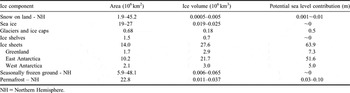
Ice and snow occur on Earth in the form of seasonal snow cover on land surfaces, floating sea ice, lake ice and river ice, permafrost and seasonally frozen ground, glaciers and ice caps at high altitude or latitude, floating ice shelves, and ice sheets. The amount of ice in these reservoirs is shown in Table I. The vast majority of the ice mass is stored in the great ice sheets of Greenland (11%) and Antarctica (88%). For the present day ocean area, the loss of about 390 km3 (about 360 Gt) of ice grounded on land will add 1 mm to global sea level. Small glaciers and ice caps, including those in polar regions, represent less than 1% of the almost 65 m potential sea level rise from ice melt (Table I).
Area, volume and potential sea level contribution of snow and ice reservoirs on the Earth. For snow, sea ice and seasonally frozen ground, the seasonal minimum and maximum are shown; the annual mean is shown for the other components. After Lemke et al. Reference Lemke, Ren, Alley, Allison, Carrasco, Flato, Fujii, Kaser, Mote, Thomas and Zhang2007, with apportioning between EAIS and WAIS based on Lythe et al. (Reference Lythe and Vaughan2001) and with values for glaciers and ice caps (including those around Antarctica and Greenland) from Houghton et al. (Reference Houghton, Ding, Griggs, Noguer, van der Linden, Dai, Maskell and Johnson2001).

NH = Northern Hemisphere.
Three ice sheets exist on Earth today, the Greenland Ice Sheet (GIS) and the West Antarctic and East Antarctic ice sheets (WAIS and EAIS), but other large ice sheets have existed in the Northern Hemisphere during the ice ages of the last ∼3 million years, and elsewhere even further back in time.
Ice sheets are formed mainly from snowfall which, at temperatures that are typically well below the melting point, metamorphoses into ice over decades to centuries. The ice sheets flow towards the coast under their own weight by internal deformation and basal sliding, transferring mass from the interior to the ocean. Inland, ice sheet flow rates may be only a few metres per year, mostly due to internal deformation. Nearer the coast ice flow is more rapid (up to hundreds or even thousands of metres per year) and often channelled into fast-moving ice streams (which flow between slower-moving ice walls) or outlet glaciers (with rock walls). In these, sliding due to lubrication by meltwater or deformable slurries of wet sediment at the base is an important component of the motion (Kamb Reference Kamb2001).
Ice streams and outlet glaciers typically feed into floating ice shelves (Antarctic Ice Sheets, AIS) and calving outlet glaciers (GIS) which are the major sites of mass loss. Around Antarctica ice shelves fringe 44% of the total coastline (Drewry et al. Reference Drewry, Jordan and Jankowski1981) covering an area of 1.5 million km2 with an average thickness of over 400 m. Ice shelves are nourished both by the ice discharged from the ice sheet and by additional snowfall on the surface. Mass loss occurs via iceberg calving, basal melting and sometimes surface melting. Large icebergs calve from the ice front where the ice shelf is typically less than 300 m thick (Lythe et al. Reference Lythe and Vaughan2001). Basal melting into the ocean cavity beneath Antarctic ice shelves can be as high as many tens of metres per year (Rignot & Jacobs Reference Rignot and Jacobs2002) beneath the deepest parts where the ice first starts to float (the grounding line) (e.g. Payne et al. Reference Payne, Holland, Shepherd, Rutt, Jenkins and Joughin2007). There are few ice shelves in Greenland, and these are confined within glacier-carved fjords. More typically, outlet glaciers have floating tongues extending a few kilometres to tens of kilometres seaward between rock walls. These can have important influences on glacier flow, as illustrated by the doubling in speed of Jakobshavn Isbrae (Joughin et al. Reference Joughin, Abdalati and Fahnestock2004) soon after thinning and breakup of its floating ice tongue (Thomas et al. Reference Thomas, Abdalati, Frederick, Krabill, Manizade and Steffen2003).
Much of the ice in the ice sheets is over 2000 m thick, and the thickest ice in EAIS is more than 4800 m (Lythe et al. Reference Lythe and Vaughan2001). The large volume of ice in the ice sheets (Table I) constitutes about 70% of all the freshwater on Earth (e.g. Gleick Reference Gleick1996). The weight of this load of ice depresses the underlying bedrock in the centre of the GIS and AIS land masses by about 30% of the ice thickness, or many hundreds of metres. WAIS differs in morphology from EAIS and GIS. Whereas EAIS and GIS rest on bedrock that is mostly above sea level, the ice in WAIS is grounded on a bed that is in places more than 2000 m below sea level. The response of such a marine ice sheet to external changes depends on interactions with the ocean as well as on other climate factors, and may be susceptible to rapid disintegration if the coastal ice thins and floats (Thomas Reference Thomas1979).
Ice sheet mass balance
Mass is continually added to the ice sheets as snowfall and removed, mostly by iceberg calving and basal melting and, for the GIS, by surface melting. The difference between the amount of mass added and that removed is called the ice sheet mass balance; any imbalance between ice gain and loss results in a change in the mass of ice stored within the ice sheet and a consequent change in global sea level.
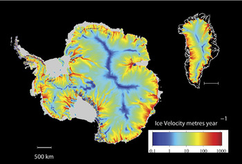
If the total mass of ice that is lost annually equals the annual mass gain, then the ice sheet is said to be “in balance”. If both the surface topography (which determines the direction of ice flow, assuming it is in the direction of the steepest slope) and the distribution of snowfall over an ice sheet are known, then the amount of ice flow necessary to maintain balance can be calculated. Combining this ice flux with measured ice thickness leads to the so-called “balance velocity” which is shown for both Antarctica and Greenland in Fig. 1. The velocity scale on this figure is logarithmic and clearly shows the individual drainage basins, the ice divides, the slow moving interior ice, the focussing of the ice into fast moving ice streams and outlet glaciers, and the acceleration of ice movement towards the coast.
Balance ice velocity for AIS (left, after Budd & Warner Reference Budd and Warner1996) and GIS (right). The surface velocity scale is logarithmic. The grey areas around Antarctica are floating ice shelves. The black coastal areas around Greenland are ice sheet-free land. Since only the flow in the main Greenland Ice Sheet was simulated, this coastal area includes some glaciers and ice caps.

Because the climate over the ice sheets is so cold, the air can hold only a small amount of moisture and snowfall rates are low. In the centre of AIS, for example, the annual snowfall represents less than 5 cm yr-1 of water, and the average over the total AIS is only about 15 cm yr-1: in terms of their precipitation, the ice sheets are deserts. Because of their vast size, however, there is still a large annual addition of snow mass. For GIS the annual gain and loss of mass is about 500 billion tonnes (Gt yr-1), and for WAIS plus EAIS the total is about 2200 Gt yr-1 (e.g. Houghton et al. Reference Houghton, Ding, Griggs, Noguer, van der Linden, Dai, Maskell and Johnson2001). These annual mass fluxes are equivalent to 1.4 mm and 6.1 mm of sea level equivalent respectively.
Changes to the ice sheet mass balance can occur with changes in the rate of snowfall or of surface melt accompanying climate change, or with changes in the rate of ice discharge. Changes in coastal discharge rates may be affected both by present climate change and by longer-term processes. Snowfall events that add mass to the ice sheets occur episodically, with considerable variability from year to year, but once incorporated in an ice sheet the snow remains as part of the ice sheet for thousands of years on average. The amount and distribution of snowfall will respond quickly to changes in weather and climate, but ice velocity over most of an ice sheet changes only slowly in response to changes in the ice sheet shape or surface temperature. Until recently, it was assumed that this was also the case in the faster moving parts of the ice sheets - the ice streams and outlet glaciers that are the main pathways of mass flux to the ocean. However, recent observations have shown that large velocity changes can occur rapidly on ice streams and outlet glaciers in response to changing basal conditions (e.g. Howat et al. Reference Howat, Joughin and Scambos2007) or changes in the ice shelves into which they flow (e.g. Rignot et al. Reference Rignot, Casassa, Gogineni, Krabill, Rivera and Thomas2004).
Because of the vast reservoirs of water mass they store, determining the role that the AIS and GIS play in current global sea level change has long been a major challenge for polar science. Until recent advances in measurement technology, however, even whether the ice sheets were gaining or losing mass was unknown. Here we summarize the status of ice sheets reported in the Fourth Assessment Report of the Intergovernmental Panel on Climate Change (AR4) and review the considerable progress that has been made since the cut-off date for work used in that report.
Past ice sheet changes and sea level
The importance of ice sheets to sea level is demonstrated by major ice sheet fluctuations in the past which are revealed by ocean sediment records and ice core records. For approximately the last million years these fluctuations have been dominated by ice age cycles of around 100 000 years, with about 10% of the time in a high sea level/low ice volume “interglacial” climate, like the present Holocene period. During past glacial periods (“ice ages”), the existing ice sheets of Greenland and Antarctica expanded, and two large ice sheets were established across North America and northern Europe. The combined effect of the water locked in these large ice sheets caused a drop of about 125 m in global sea level (Fleming et al. Reference Fleming, Johnston, Zwartz, Yokoyama, Lambeck and Chappell1998). The record of past ice ages shows that ice sheets shrink in response to warming and grow in response to cooling, and that the shrinkage can be far faster than growth. This occurs because surface melting rates can be much larger than snowfall rates, and because ice discharge may be accelerated by processes such as enhanced basal lubrication, or by the removal of restraint to flow when marginal ice shelves disintegrate. The glacial cycles are believed to have been driven by small changes of the Earth’s orbital geometry, causing subtle changes in the amount, distribution and timing of incoming solar radiation. This small effect was amplified by processes such as changes in the reflectivity of the ground when covered by ice or snow (albedo feedback), and addition or removal of carbon dioxide (a greenhouse gas) from the atmosphere (for example by absorption into a cooler ocean and other oceanic processes).
Ice core records show that some previous interglacial periods have been colder than present and some apparently warmer. This is to be expected, since the net result of the astronomical modulations varies within the overall cycle. Past temperatures recorded by ice cores also partly reflect changes in elevation of the ice sheet relative to sea level.
The best available data for a past interglacial are for the most recent one (also referred to as the Eemian or the Last Inter-Glacial, LIG), which occurred around 125 000 years ago. At the peak of the LIG, summer temperatures in the Arctic are thought to have been around 2°C warmer than present (although with notable spatial variability) and sea level was at least 4–6 m higher than present (Overpeck et al. Reference Overpeck, Otto-Bliesner, Miller, Muhs, Alley and Kiehl2006, Otto-Bliesner et al. Reference Otto-Bliesner, Marsall, Overpeck, Miller and Hu2006). While there would be small contributions from mountain glacier melt and Arctic ice fields, the bulk of that sea level rise must have been from GIS and AIS contributions. Estimates of the LIG sea level contribution from the GIS have ranged from 4–5.5 m (Cuffey & Marshall Reference Cuffey and Marshall2000), through 3.5–4.5 m (Lhomme et al. Reference Lhomme, Clarke and Marshall2005) and 2.2–3.4 m (Overpeck et al. Reference Overpeck, Otto-Bliesner, Miller, Muhs, Alley and Kiehl2006) to only 1–2 m (Oerlemans et al. Reference Oerlemans, Dahl-Jensen and Masson-Delmotte2006). The balance of the increase must have come from Antarctica and, if the total sea level rise was greater than 6 m as Overpeck et al. (Reference Overpeck, Otto-Bliesner, Miller, Muhs, Alley and Kiehl2006) consider possible, then the Antarctic contribution must have been even greater.
The rate of change of sea level during the last interglacial is also relevant to what may happen in the future. An LIG rise of 4–6 m or more may have occurred gradually, or with abrupt steps as ice sheets collapsed due to rapid processes. Recent work based on marine sediment and coral data (Rohling et al. Reference Rohling, Grant, Hemleben, Siddall, Hoogakker, Bolshaw and Kucera2008) shows periods of sea level rise at rates of 1.6 m per century during the LIG.
After the peak of the last ice age (the “glacial maximum”) ∼21 000 years ago, sea level rose at rates which appear to peak at more than 3 m per century (Houghton et al. Reference Houghton, Ding, Griggs, Noguer, van der Linden, Dai, Maskell and Johnson2001). Sea level variation over glacial cycles was predominantly driven by the growth and melting of ice on land with only a small fraction of the contribution coming from thermal expansion or contraction of seawater. At about 2000 years before present (bp), sea level rise had almost ceased and, from 1000 yrs bp to the late 19th century, sea level variation was confined within a range of about 0.2 m.
Recent rates of sea level rise
From 1850–99 to 2001–05, global temperature increased by 0.76°C (Solomon et al. Reference Solomon, Qin, Manning, Chen, Marquis, Averyt, Tignor and Miller2007), leading to warming of the oceans and melting of ice on land. Church & White (Reference Church and White2006) used a combination of tide gauge records and satellite-altimeter data to reconstruct sea level from 1870 to 2004, showing a global-average rise of 0.17 m during the 20th century. Records also suggest an acceleration of sea level rise from about zero rate of rise around the start of the 19th century, to a rate of 1.8 mm yr-1 from 1961 to 2003, and 3.1 mm yr-1 over the period 1993 to 2003.
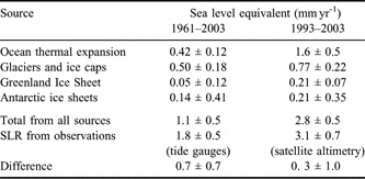
Unlike the sea level variations associated with the glacial-interglacial cycles, thermal expansion of a warming ocean played an important role in 20th century sea level rise (SLR). The AR4 (Solomon et al. Reference Solomon, Qin, Manning, Chen, Marquis, Averyt, Tignor and Miller2007) estimated that the two largest contributions to 20th century SLR were thermal expansion and the melting of glaciers and ice caps (excluding Greenland and Antarctica) (Table II). Thermal expansion of ocean water was estimated by AR4 to account for 0.4 mm yr-1 of SLR for the period 1961–2003 and to have risen to 1.6 mm yr-1 for the period 1993–2003. The most important source of the remainder of the SLR is melting of ice on land in glaciers, ice caps and ice sheets. Glaciers in most mountain regions are retreating, and a recent assessment has suggested that the contribution from ice caps and glaciers is accelerating, and had reached 1.1 mm yr-1 in 2006 (Meier et al. Reference Meier, Dyurgerov, Rick, O’Neel, Pfeffer, Anderson, Anderson and Glazovsky2007).
Contributions to the rate of sea level rise estimated by AR4 (Solomon et al. Reference Solomon, Qin, Manning, Chen, Marquis, Averyt, Tignor and Miller2007).

For the period 1961–2003, comparison of measured SLR with the thermal expansion and cryospheric contributions in Table II leaves an unexplained contribution of 0.7 ± 0.7 mm yr-1. By using statistical techniques to interpolate sparse observations, correcting systematic errors in temperature observations, and making allowance for the contribution from the deep ocean, Domingues et al. (Reference Domingues, Church, White, Gleckler, Wijffels, Barker and Dunn2008) estimate a revised thermal expansion for 1961–2003 of 0.7 mm yr-1 and obtain improved closure of the sea level budget over multi-decadal periods. For the period 1993–2003, the estimated global sea level budget is closed within error limits and the AR4 (Solomon et al. Reference Solomon, Qin, Manning, Chen, Marquis, Averyt, Tignor and Miller2007) was able, for the first time, to conclude that, taken together, GIS and AIS are likely (more than 90% probability) to have contributed to sea level rise at an average rate of about 0.4 mm yr-1 over this period. For GIS, thickening in central regions has been more than offset by increased melting and thinning near the coast. Flow speed has also increased for some GIS outlet glaciers, which drain ice from the interior. In Antarctica mass loss occurred mostly along coastal sectors of the Antarctic Peninsula and in WAIS. Recent accelerations in ice flow explain much of this loss. Over the interior of EAIS there has been some slight thickening, which seems to be associated with higher accumulation rates.
Methods of estimating ice sheet mass balance
The ice sheets are composed of many separate ice drainage basins defined by surface topography, analogous to river drainage basins. These respond with different time scales and to spatially varying patterns of snowfall. In some the total ice mass may be increasing, while in others it may be decreasing, and the mass balance of the entire ice sheet is the sum of all the separate components. There are two observational methods of estimating the mass balance of an ice sheet, the integrated method and the flux component method (Jacka et al. Reference Jacka2004), explained in more detail below. Recent results using these techniques (since AR4) are discussed later.
Integrated method
In the integrated method, direct estimations of the change in i) elevation, or ii) mass of the ice sheet with time are made over an entire ice sheet (or an individual ice drainage basin). This is done using airborne or satellite remote-sensing technologies that have been developed, mostly over the last two decades.
i) Elevation: Ice sheet surface elevation is mapped using radar or laser altimeters on aircraft and satellites to measure the distance from the instrument to the surface, together with precise information on the location of the altimeter. Radar altimeter signals penetrate the near-surface snow and ice layer, and the results can be affected by the internal structure. Satellite-borne radar altimeters have a relatively large footprint (2–3 km), which can lead to a bias over rough or sloping terrain, and challenge measurement accuracy in narrower outlet glaciers. Laser altimeter signals are directly reflected from the surface, have a smaller footprint (tens of metres) and provide higher resolution data than radars, although they are unable to penetrate thick cloud cover, and undergo forward scattering when thinner clouds are present.
The Earth’s crust under the ice sheets, especially AIS, is rising slowly, still adjusting to the removal of ice load since the peak of the last ice age 21 000 years ago. Measured changes in ice sheet surface elevation must be corrected for this glacial isostatic adjustment (GIA). To then convert the volume change into mass change, allowance must be made for any changes in the density profile of the ice that have occurred. A recent study for Antarctica has shown that density changes due to decadal-scale variations in snowfall rate and surface temperature can have an impact on surface elevation of comparable magnitude to the measured altimeter changes (Helsen et al. Reference Helsen, van den Broeke, van de Wal, van de Berg, van Meijgaard, Davis, Li and Goodwin2008), complicating the interpretation of altimeter surveys.
ii) Mass: Change of mass of the ice sheets directly affects the regional gravitational field. Ice sheet mass change has been detected using satellites to measure gravitational field changes by precisely monitoring the separation between a pair of satellites travelling c. 200 km apart in virtually identical orbits (the Gravity Recovery and Climate Experiment (GRACE) satellite mission). These techniques show considerable sensitivity in estimating mass change on a month-by-month basis, but to date different analysis techniques give somewhat different results. Again it is necessary to correct for the GIA which moves crustal mass and has a large impact on the total mass in a region beneath the satellite orbit. Satellite gravity observations have only been made for a few years and ice sheet changes detected may reflect inter-annual variability as well as any trend.
Flux component method
The flux component method requires estimation of the difference between the sum of all the mass inputs to the ice sheet and the sum of all the outputs. This can be done for the whole ice sheet or for individual drainage basins.
Since any imbalance in the ice sheet mass balance is typically only a small fraction of the total input and output fluxes it is difficult to estimate the difference with great accuracy. An imbalance corresponding to 5% of the Antarctic ice sheet accumulation or discharge corresponds to about 0.3 mm yr-1 of sea level change. However the measurements required for the flux component method also provide information on the processes of ice deposition, transport, melting and discharge. Quantitative descriptions of these processes are essential to make projections of future changes, whereas the integrated method reveals only the current status.
Estimation of the mass input requires comprehensive knowledge of the spatially and temporally varying pattern of snow accumulation. In situ observations of mass input include direct measurements of snow accumulation against marker poles, which give short temporal records, and interpretation of snow-pits and ice cores, which provide longer climatological records. Available data are sparse, and large areas of the ice sheets remain unsurveyed, so it is necessary to use other techniques to interpolate the accumulation pattern between survey sites. Surface-based ground penetrating radar surveys can be used to track past accumulation horizons over long distances. Satellite passive microwave measurements provide information on the microstructure of the surface snow, which is related to the accumulation rate, and have also been used to interpolate between direct measurements (Vaughan et al. Reference Vaughan, Bamber, Giovinetto, Russell and Cooper1999, Arthern et al. Reference Arthern, Winebrenner and Vaughan2006).
Recently, computer models of regional atmospheric circulation have been used to simulate the snowfall patterns over the ice sheets (e.g. van de Berg et al. Reference van de Berg, van den Broeke, Reijmer and van Meijgaard2006). These relatively high resolution regional models are driven by the outputs from global weather forecasting models for recent decades. They have demonstrated good general agreement with the sparse in situ observations. Summer melting of snow and ice in coastal regions, which is particularly important in Greenland, can also be well represented by melt and runoff models driven by outputs from the meteorological models (e.g. Hanna et al. Reference Hanna, Huybrechts, Steffen, Cappelen, Huff, Shuman, Irvine-Fynn, Wise and Griffiths2008).
The loss by outflow is usually estimated as the ice discharge across the grounding line of the ice sheet, since this is what matters for sea level. This requires observations of the speed of ice flow and the thickness of the column of moving ice. Satellite observations have been used to provide wide coverage of ice surface velocities (e.g. Jezek Reference Jezek2008). The velocity of an ice sheet varies with depth, and the average velocity of an ice column is usually less than the surface velocity. This contributes a further level of uncertainty to the discharge estimates; although this effect is less important in ice streams and outlet glaciers which move mostly by basal sliding and which discharge most of the ice.
A check on the accuracy of estimates of ice sheet mass change can also be gained from the total sea level budget. Global average sea level rise is now monitored accurately from space, and the residual between the observed rate of change and the sum of the individual components (thermal expansion, mass loss from glaciers and ice caps, mass loss from ice sheets, and changes to ground-water storage) provides an assessment of accuracy of the component estimates (e.g. Cazenave et al. Reference Cazenave, Dominh, Guinehut, Berthier, Llovel, Ramillien, Ablain and Larnicol2009).
Updated estimates of ice sheet mass balance since the IPCC AR4
Satellite techniques are providing increasingly accurate evidence of the current contribution of ice sheets to sea level rise. Since the cut-off date in the latter part of 2005 for work assessed by the IPCC AR4, a number of further studies of the mass balance of Greenland and Antarctica have been made using satellite altimetry, satellite gravity measurements and estimates of mass influx and discharge from a variety of techniques. Considerable errors and uncertainties remain in these assessments, but a consistent picture is emerging of mass loss from GIS and AIS that contributes to sea level rise. Progress since AR4 has been sufficient to generate several reviews on the contribution of ice sheets to sea level rise, including publications by Oerlemans et al. (Reference Oerlemans, Dahl-Jensen and Masson-Delmotte2006), Alley et al. (Reference Alley, Spencer and Anandakrishnan2007), Bentley et al. (Reference Bentley, Thomas and Velicogna2007), Shepherd & Wingham (Reference Shepherd and Wingham2007) and Bell (Reference Bell2008).
Greenland
Integrated method
A number of different analyses of GRACE data consistently give a picture of mass loss from Greenland over the last few years, although the magnitude of the loss varies between different analyses. Velicogna & Wahr (Reference Velicogna and Wahr2005) estimated a net loss rate of 75±20 Gt yr-1 (equivalent to nearly 0.2 mm of SLR) between April 2002 and July 2004 and a much larger loss of 227±33 Gt yr-1 (0.6 mm SLR) over the period April 2002–April 2006 (Velicogna & Wahr Reference Velicogna and Wahr2006a), suggesting a substantial increase in mass loss, most of which occurred in the southern part of the ice sheet. For the period July 2002–March 2005, Ramillien et al. (Reference Ramillien, Lombard, Cazenave, Ivins, Llubes, Remy and Biancale2006) estimated a mass loss using the GRACE data of 128±15 Gt yr-1. The analysis technique used in these studies gives estimates spatially averaged over large regions (∼400 km ground resolution) of the ice sheets. Luthcke et al. (Reference Luthcke, Zwally, Abdalati, Rowlands, Ray, Nerem, Lemoine, McCarthy and Chinn2006) used a different technique with finer spatial resolution to resolve changes in different drainage basins and at different elevation ranges for the period July 2003–July 2005. They estimated a Greenland mass gain of 54 Gt yr-1 above 2000 m surface elevation and a mass loss of 155 Gt yr-1 below 2000 m, yielding a net loss of 101±16 Gt yr-1. Again, most of the net mass loss occurred in drainage basins in the south of Greenland.
Wouters et al. (Reference Wouters, Chambers and Schrama2008) analysed five years of GRACE observations at finer scale, and argue that some of the previous differing gravity-based estimates represent changing rates over time, rather than just differences in methodology. For 2003–2008 they estimate an average loss rate of 179±25 Gt yr-1, but also demonstrate considerable year-to-year variation, particularly in the summer seasonal ice loss, suggesting that long-term studies will be essential for confirmation of any trends. Also for the 2003–08 period, Cazenave et al. (Reference Cazenave, Dominh, Guinehut, Berthier, Llovel, Ramillien, Ablain and Larnicol2009) estimate a loss of 136±18 Gt yr-1, and comment that the reasons for discrepancies between the different analyses are as yet unclear.
Flux component method
In Greenland there is a pattern of near-coastal thinning of the ice sheet primarily in the south along fast-moving outlet glaciers (Rignot & Kanagaratnam Reference Rignot and Kanagaratnam2006, Howat et al. Reference Howat, Joughin and Scambos2007) which is partially, but not fully, compensated by thickening at higher elevations. While the acceleration of some major outlet glaciers appears to have been transient, Howat et al. (Reference Howat, Smith, Joughin and Scambos2008) show that in south-east Greenland many smaller drainage basins are also contributing to ice loss, especially the catchments of marine-terminating outlet glaciers. Although outlet glacier trunks are thinning most rapidly, the dominant loss is from slower thinning dispersed over large inland areas. Near-coastal surface melt and runoff have increased significantly since 1960 in response to warming temperature, but total snow precipitation has also increased (Hanna et al. Reference Hanna, Huybrechts, Steffen, Cappelen, Huff, Shuman, Irvine-Fynn, Wise and Griffiths2008). The average GIS surface temperature rose by more than 1.5°C over the period 2000–06 and mass loss estimated from GRACE gravity data commenced within 15 days of the initiation of surface melt, suggesting that the water drains rapidly from the ice sheet (Hall et al. Reference Hall, Williams, Luthcke and Digirolamo2008).
Rignot et al. (Reference Rignot, Box, Burgess and Hanna2008a) used an empirical method to estimate the flux component mass balance of the Greenland Ice Sheet, year by year, from 1958 to 2007. They show that for eight years for which estimates of total mass discharge are available from Greenland, the anomalies in that discharge were linearly correlated with anomalies in the net surface mass budget. They hypothesize that this relationship holds because in years when there is more surface melt, the ice thins and partially floats near the front, reducing the buttressing of inland ice (Thomas Reference Thomas2004) and increasing outflow. Annual surface mass budget values for the period 1957–2007 were obtained for a combination of two prior estimates, Box et al. (Reference Box, Bromwich, Veenhuis, Bai, Stroeve, Rogers, Steffen, Haran and Wang2006) and Hanna et al. (Reference Hanna, Huybrechts, Steffen, Cappelen, Huff, Shuman, Irvine-Fynn, Wise and Griffiths2008), both of which use temperature (to estimate melt) and snowfall from meteorological models. The total annual mass balance reconstructed by Rignot et al. (Reference Rignot, Box, Burgess and Hanna2008a) shows that the ice sheet was losing around 100 Gt yr-1 during the 1960s, was approximately in balance during the 1970s and 1980s and since 1997 has been increasingly losing mass. These Greenland mass balance estimates from Rignot et al. (Reference Rignot, Box, Burgess and Hanna2008a) for the period 1992–2007 are shown in Fig. 2, averaged over 5–6 year periods.
Estimates of the net mass budget of the Greenland Ice Sheet since 1992. Adapted from Thomas et al. (Reference Thomas, Davis, Frederick, Krabill, Li, Manizade and Martin2008). See text for details, and the appendix for sources of the numbered estimates.

Figure 2 shows estimates of the mass balance of the GIS that have been made since the early 1990s. In this representation, the horizontal dimension of the boxes shows the time period over which the estimate was made, and the vertical dimension shows the upper and lower limits of the estimate. The colours represent the different methods that were used: black is satellite radar altimetry, orange is aircraft laser altimetry, purple is aircraft/satellite laser altimetry, red is the flux component method, and blue is satellite gravity. The dashed green box represents the estimated Greenland balance of IPCC AR4. These data indicate that mass loss from the GIS may be increasing, although it is also clear that the various estimates are frequently not in agreement. It is important however to note that there can be large variability from year to year in the surface melt in Greenland and the short term changes, from GRACE data in particular, which are only available since 2003, may reflect this rather than a long-term trend (Wouters et al. Reference Wouters, Chambers and Schrama2008).
Antarctica
Integrated method
i) Surface elevation: In Antarctica, Zwally et al. (Reference Zwally, Giovinetto, Li, Cornejo, Beckley, Brenner, Saba and Yi2005) used satellite radar altimetry to estimate a net loss in WAIS of 47±4 Gt yr-1, and a net gain in EAIS of 17±11 Gt yr-1 over the period 1993–2003. The radar altimeter data do not cover the immediate area around the pole so data were interpolated to this region. Davis et al. (Reference Davis, Li, McConnell, Frey and Hanna2005) also showed the same general pattern of EAIS thickening and WAIS thinning with the same satellite radar data. They argued that the EAIS change was due to increased snowfall, although Monaghan et al. (Reference Monaghan2006) found no evidence of systematic change in snowfall over the last 50 years in a record they derived from meteorological records and ice core data. The Monaghan et al. (Reference Monaghan2006) conclusion is not inconsistent with that of Davis et al. (Reference Davis, Li, McConnell, Frey and Hanna2005) if a snowfall increase occurred earlier than 50 years ago.
ii) Mass: From the GRACE satellite gravity data between April 2002 and July 2005, Velicogna & Wahr (Reference Velicogna and Wahr2006b) estimated a net loss rate from the AIS, including the Antarctic Peninsula and small glaciers, of 139±73 Gt yr-1. A pattern of near balance for EAIS, and mass loss from WAIS was also seen in these data. Ramillien et al. (Reference Ramillien, Lombard, Cazenave, Ivins, Llubes, Remy and Biancale2006) estimated EAIS mass gain of 67±28 Gt yr-1 and WAIS loss of 107±23 Gt yr-1 from GRACE data for July 2002–March 2005. Cazenave et al. (Reference Cazenave, Dominh, Guinehut, Berthier, Llovel, Ramillien, Ablain and Larnicol2009) estimated an average loss for all of Antarctica of 198±22 Gt yr-1 for the five year period 2003–2008. The GIA correction for AIS is larger than for GIS, and poorly known: it is a major source of uncertainty in these Antarctic estimates.
Flux component method
Rignot et al. (Reference Rignot, Bamber, van den Broeke, Davis, Li, van de Berg and van Meijgaard2008b) determined the ice discharge across 85% of the coastline of Antarctica using satellite data. They used radar interferometry to measure the surface velocity of the ice and estimated the ice thickness at the grounding line, where it starts to float, from surface elevation measurements and the assumption of hydrostatic equilibrium. With snowfall estimates from meteorological modelling (van de Berg et al. Reference van de Berg, van den Broeke, Reijmer and van Meijgaard2006) they were able to apply the flux method to estimate the mass balance of most of the Antarctic drainage basins. For the year 2000 the overall mass balance was essentially zero for EAIS (-4±61 Gt yr-1) but with mass losses in WAIS (-106±60 Gt yr-1) and perhaps along the Antarctic Peninsula (-28±45 Gt yr-1). For some regions velocity observations from different epochs were used to explore changes in ice discharge.
The Rignot et al. (Reference Rignot, Bamber, van den Broeke, Davis, Li, van de Berg and van Meijgaard2008b) flux balance study showed that ice loss from WAIS was large in the basins draining into the Bellingshausen and Amundsen seas where glaciers have been previously observed to accelerate (Joughin et al. Reference Joughin, Rignot, Rosanova, Lucchitta and Bohlander2003, Shepherd et al. Reference Shepherd, Wingham and Rignot2004). The ice discharge in this region increased between 1996 and 2006, increasing the net mass loss over the period by 59%. The rate of loss from the Antarctic Peninsula has also increased to 60±46 Gt yr-1. In EAIS some small loss is occurring in drainage basins such as the Totten Glacier basin in Wilkes Land, but is offset by gain elsewhere (Rignot et al. Reference Rignot, Bamber, van den Broeke, Davis, Li, van de Berg and van Meijgaard2008b).
The Antarctic Peninsula region resembles other mountainous glaciated regions, and arguably the numerous glaciers require separate consideration from the EAIS and WAIS. This region has experienced much greater warming than the continent as a whole - over 3°C in the past fifty years (Meredith & King Reference Meredith and King2005). This has led to widespread retreat (Cook et al. Reference Cook, Fox, Vaughan and Ferrigno2005) and acceleration (Pritchard & Vaughan Reference Pritchard and Vaughan2007) of the tidewater glaciers. Pritchard & Vaughan (Reference Pritchard and Vaughan2007) estimate the mass loss from the Peninsula around 2005 as 52±20 Gt yr-1.
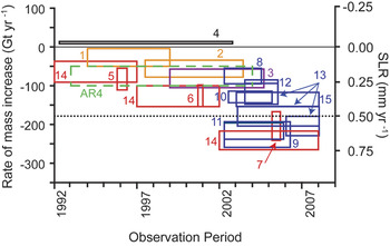
Figure 3 shows estimates of the mass balance of the Antarctic Ice Sheet that have been made since the early 1990s. Again, the horizontal dimension of the boxes shows the time period over which the estimate was made, and the vertical dimension shows the upper and lower limits of the estimate. The colours represent the different methods that were used: black is satellite radar altimetry, red is the flux component method, and blue is satellite gravity. The dashed green box represents the estimated Antarctic balance of IPCC AR4. The uncertainties are such that there is no strong evidence for increasing Antarctic loss over the period shown.
Estimates of the net mass balance of the Antarctic Ice Sheet since 1992. Adapted from Bentley et al. (Reference Bentley, Thomas and Velicogna2007). See text for details, and the appendix for sources of the numbered estimates.

Projections of future sea level rise
Future sea level rise will be a result of global climate change with significant and long-term environmental, social, cultural and economic consequences for human society. Many of the world’s largest cities are built in low-lying coastal regions, and it is expected that sea level rise by the end of the 21st century will affect tens of million people globally (e.g. Nicholls et al. Reference Nicholls, Wong, Burkett, Codignotto, Hay, McLean, Ragoonaden and Woodroffe2007). In addition to possible changes in the frequency and intensity of extreme events such as storm surges and tropical cyclones, sea level rise will result in increased frequency of severe flooding events and coastal erosion.
The IPCC Third Assessment Report (TAR; Houghton et al. 2001) and the AR4 made projections of future sea level for a wide range of scenarios of future greenhouse gas emission. These IPCC projections are derived from quantitative computer models based on the best available understanding of the physics of the climate system, and include sea level contributions from ocean thermal expansion, glacier and ice cap melting, and from some, but not all, potential changes to the Greenland and Antarctic ice sheets. The models were driven by different societal projections of future greenhouse gas emissions (Nakicenovic & Swart Reference Nakicenovic and Swart2000). But any dynamic response of AIS and GIS to climate change, which is not adequately represented in the ice sheet models used by IPCC, was treated only empirically, and in different ways in each of the reports.
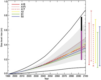
The TAR time-varying SLR projections, averaged over a number of different climate models, are shown in Fig. 4 as curved coloured lines for six emission scenarios (indicated by the letters at the top left; see Nakicenovic & Swart Reference Nakicenovic and Swart2000). The thin, coloured bars at the right of the diagram show the range of predictions from the different models for each of these scenarios (Houghton et al. Reference Houghton, Ding, Griggs, Noguer, van der Linden, Dai, Maskell and Johnson2001). The region in dark grey shading shows the range of the average of the models for 35 emission scenarios, and the region in lighter shading shows the range of all models for all 35 scenarios. These projections do not include additional uncertainties due to land ice, permafrost and ocean sedimentation processes, and the TAR projections account for these by expanding the SLR range to the outermost black lines in Fig. 4 (Houghton et al. Reference Houghton, Ding, Griggs, Noguer, van der Linden, Dai, Maskell and Johnson2001). These expanded error limits did not include rapid dynamical change to WAIS: TAR considered WAIS disintegration within a century as unlikely (Houghton et al. Reference Houghton, Ding, Griggs, Noguer, van der Linden, Dai, Maskell and Johnson2001). At 2100 there is a large range of uncertainty in the TAR SLR projections, from slightly less than 0.1 m to nearly 0.9 m.
IPCC TAR, and IPCC AR4 projections of sea level rise for the 21st century. The TAR projections for different greenhouse gas emission scenarios are shown as the series of curved lines; the AR4 projection for the period 2090–2099 is shown by the pink and black bars. See text for further details. After Church et al. Reference Church, White, Aarup, Wilson, Woodworth, Domingues, Hunter and Lambeck2008.

AR4 also made emission-scenario based projections for SLR projections for well-quantified processes but “excluding future rapid dynamical changes in ice flow” (table SPM.3; IPCC 2007) “because a basis in published literature is lacking” (p. SPM-14; IPCC 2007). The quantified processes included changes to the surface mass budget of the ice sheets, and ice flow response to changing topography. Ice sheet imbalances that have recently occurred due to accelerated ice flow were also factored in by assuming that they will continue to contribute to SLR at the same rate over the projection period. The quantified AR4 range of projections for SLR at 2095 (actually 2090–2099) is shown in Fig. 4 as a vertical pink bar. To account for any future dynamical response of the ice sheets, AR4 used the heuristic argument that an additional imbalance might scale with future temperature increase. Based on a measured increase in SLR of 0.32 mm yr-1 with recent global temperature increase, this was estimated to add an additional 0.1–0.2 m of SLR by 2095 (Solomon et al. Reference Solomon, Qin, Manning, Chen, Marquis, Averyt, Tignor and Miller2007). This is shown as the black vertical bar on Fig. 4. AR4 also added a significant caveat that even greater sea level rise from the AIS and GIS cannot be excluded.
The lower limit of the AR4 projections (0.18 m) is somewhat greater than the lowest TAR estimate. The quantified AR4 upper limit at 2095 (0.59 m, without the empirically estimated ice sheet factor) is less than the TAR upper limit. However with consideration of the AR4 ice sheet scaling factor, the upper ranges of the two sea level projections are similar.
The dynamic response of ice sheets to global warming is the largest unknown in the projections of sea level rise over the next century. Rahmstorf (Reference Rahmstorf2007) made a semi-empirical projection for strong future warming scenarios of a SLR of over 1 m by 2100. This is consistent with what happened during warming in the LIG and cannot be ruled out. The LIG warming was caused by perturbations of Earth’s orbit (Overpeck et al. Reference Overpeck, Otto-Bliesner, Miller, Muhs, Alley and Kiehl2006) and arrived much more gradually than is projected for human-induced warming, so a faster sea level rise in the future than at the LIG would not be surprising. Observed sea level change between 1993 and 2006 was close to the upper limit of the IPCC TAR projections (Rahmstorf et al. Reference Rahmstorf, Cazenave, Church, Hansen, Keeling, Parker and Somerville2007).
There have also been suggestions that sea level rise over the next century could be very much higher than the IPCC projections. Hansen (Reference Hansen2007) argues that the rate of increase in sea level rise will be non-linear rather than linear as observed over the past century (Rahmstorf Reference Rahmstorf2007). Assuming a ten-year doubling time for the non linear response yields a sea level rise by the end of this century of “the order of 5 metres” (Hansen Reference Hansen2007). This is consistent with estimates of the rate of rise at the end of the last ice age, although there were larger decaying ice sheets contributing to SLR then. The Hansen (Reference Hansen2007) example is based on empirical projection and not on an understanding of physical processes that might cause rapid ice sheet decay. Pfeffer et al. (Reference Pfeffer, Harper and O’Neel2008) showed that for such a large sea level rise to occur by 2100, outlet glacier flow rates would need to immediately increase greatly to speeds considered glaciologically unfeasible. Using the AR4 projections of ocean thermal expansion, and an ice flow acceleration they believed was physically possible, Pfeffer et al. (Reference Pfeffer, Harper and O’Neel2008) estimated that total SLR by 2100 could be in the range of 0.8 to 2.0 m, with the most plausible value regarded as closer to 0.8 m.
Improving ice sheet models for projecting future sea level rise
Most of the processes that affect how rapidly ice sheets will respond to future global warming are not properly accounted for in many current ice sheet models (Vaughan & Arthern Reference Vaughan and Arthern2007). The long-accepted idea that ice sheets evolve slowly has been challenged by the realization that processes that matter in the ice sheets can occur on short timescales (Truffer & Fahnestock Reference Truffer and Fahnestock2007). The three main physical processes not adequately treated in the models used for the IPCC AR4 are: 1) the flow transition from ice sheet to floating ice shelf, 2) the dynamics of rapidly flowing ice streams and outlet glaciers, and 3) the effect of basal melt water on ice dynamic processes. These dynamic processes could lead to a more rapid decay of the WAIS and GIS, which would increase the rate of sea level rise above the current IPCC projections.
Flow transition from ice sheet to floating ice
Antarctic ice shelves experience high rates of ice loss from ocean-driven basal melting near the grounding line (Rignot & Jacobs Reference Rignot and Jacobs2002), and are likely to be sensitive to changes in ocean temperatures (Williams et al. Reference Williams, Warner and Budd2002, Holland et al. Reference Holland, Jenkins and Holland2008a). A number of ice shelves along the Antarctic Peninsula, where there has been pronounced regional warming over the last 50 years, have disintegrated, sometimes in a short time. In March 2002, a 3250 km2 section of the Larsen B Ice Shelf on the eastern side of the Antarctic Peninsula broke up completely in just five weeks (Scambos et al. Reference Scambos, Hulbe and Fahnestock2003). In February and June 2008, the Wilkins Ice Shelf underwent two disintegration events on its western side, losing over 500 km2 in what is possibly the start of its complete decay (Humbert & Braun Reference Humbert and Braun2008, Scambos et al. Reference Scambos, Fricker, Liu, Bohlander, Fastook, Sargent, Massom and Wu2009). Because ice shelves are already floating, they do not affect sea level significantly when they melt. But following the collapse of the Larsen B Ice Shelf, the glaciers formerly flowing into this ice shelf accelerated by as much as eight-fold (Rignot et al. Reference Rignot, Casassa, Gogineni, Krabill, Rivera and Thomas2004, Scambos et al. Reference Scambos, Bohlander, Shuman and Skvarca2004), draining more grounded ice into the ocean and thus contributing to sea level rise. Such observations of enhanced flow rates in glaciers feeding ice shelves after they have collapsed support the hypothesis that ice shelves “buttress” the flow of the grounded ice. This implies that ice shelves and their feeder glaciers are tightly coupled, and the demise of ice shelves could lead to increased ice discharge at the grounding line, as well as grounding line retreat (Hughes Reference Hughes1973, Thomas Reference Thomas1977, Mercer Reference Mercer1978, Dupont & Alley Reference Dupont and Alley2005).
Ice shelf buttressing is not properly accounted for in current ice sheet models. This is primarily because, for computational efficiency, the models use a simple formulation of the driving stresses within the ice that does not allow for longitudinal stress gradients. This precludes them being able to account for buttressing, or predict an accelerated discharge following a collapse event. There is good understanding of the physical processes involved in this effect, and the next generation of ice sheet models that is being developed now will include the role of longitudinal stresses in the ice sheets to account for ice sheet–ice stream–ice shelf transition and the buttressing effect of ice shelves. These models will also have improved spatial resolution and will hence better resolve the ice streams that drain most of the grounded ice (Fig. 1).
Rapidly flowing ice streams and outlet glaciers
There are also other processes affecting ice sheet dynamics that are not well understood. The central parts of the AIS and GIS have been observed to change only slowly, but near the coast rapid changes over quite large areas have been observed. The concept of possible rapid disintegration of the marine WAIS was first suggested more than 30 years ago (Hughes Reference Hughes1973, Weertman Reference Weertman1976, Mercer Reference Mercer1978). Where the bedrock under a marine ice sheet slopes down towards the interior, the ice sheet may be unstable: a small retreat could in theory destabilize the entire WAIS leading to rapid disintegration. There are recent observations of significant changes occurring in the Amundsen Sea sector of WAIS. Pine Island Glacier has accelerated 38% since 1975, with most of the increase taking place over the last decade, and is now draining far more ice into the ocean than is gained upstream from snow accumulation (Rignot Reference Rignot2006). The neighbouring Thwaites Glacier is also undergoing significant dynamic change.
Many of the outlet glaciers in southern Greenland have also increased their rate of flow significantly during the past decade or so. On the west coast of Greenland the largest outlet stream, Jakobshavn Isbræ, accelerated greatly, from 5.7 km yr-1 in 1992 to 12.6 km yr-1 in 2003 (Joughin et al. Reference Joughin, Abdalati and Fahnestock2004), reversing an earlier slowdown. It shows seasonal variations in speed that are in phase with seasonal changes in the length of the floating tongue (which is really a small ice shelf embayed in a fjord), indicating a buttressing effect as for other ice shelves (Thomas Reference Thomas2004, Joughin et al. Reference Joughin, Das, King, Smith, Howat and Moon2008). Jakobshavn has had other, lower magnitude periods of acceleration and thinning during the 20th century (Csatho et al. Reference Csatho, Schenk, van der Veen and Krabill2008). Holland et al. (Reference Holland, Thomas, De Young, Ribergaard and Lyberth2008b) suggest that these are driven by occasions when warmer ocean water reaches the base of the floating glacier tongue. This indicates a strong sensitivity to ocean temperatures, even if the present warming is not necessarily a reflection of global ocean warming.
The effect of basal meltwater on ice dynamic processes
On GIS there is increasing surface melting and evidence that this meltwater from surface lakes and streams is making its way to the base of the ice sheet (the hydrofracture mechanism; Alley et al. Reference Alley, Dupont, Parizek and Anandakrishnan2005, Das et al. Reference Das, Joughin, Behn, Howat, King, Lizarralde and Bhatia2008), possibly seasonally lubricating the ice sheet flow. Zwally et al. (Reference Zwally, Abdalati, Herring, Larson, Saba and Steffen2002) observed seasonal speed-up in flow of 5–28%, correlated with summer melting, at the Swiss Camp site where annual flow is around 120 m yr-1. Price et al. (Reference Price, Payne, Catania and Neumann2008) suggest that the effects seen at Swiss Camp could be explained as a non-local upstream consequence of hydrofracture occurring only in thinner ice near the coast. More rapid movement of portions of the ice sheet during the summer melt season and an increased number of glacial “ice-quakes” have been observed (Ekstrom et al. Reference Ekstrom, Nettles and Tsai2006). Joughin et al. (Reference Joughin, Das, King, Smith, Howat and Moon2008) report a 48% seasonal acceleration of the slow-moving near-coastal ice sheet flow (regions where surface velocity is less than 150 m yr-1) but a much lesser acceleration of only 9% in outlet glacier regions where the velocities averaged 594 m yr-1. Das et al. (Reference Das, Joughin, Behn, Howat, King, Lizarralde and Bhatia2008) report the rapid drainage of a supraglacial lake through a kilometre of ice by hydrofracture, but suggest that efficient subglacial drainage may limit the influence of this on ice flow. Nick et al. (Reference Nick, Vieli, Howat and Joughin2009) use a numerical model of the Hellheim Glacier basin to simulate the response of that glacier to perturbations of the calving front and to the supply of meltwater at the base. Their study shows that observed thinning and retreat in Hellheim Glacier can be well simulated by changes to the terminus that are propagated upstream, but that the observed changes are unlikely to be caused by increased basal lubrication.
While there is currently uncertainty about the importance of such melt-driven processes and their action in thick ice, they potentially represent an additional avenue for rapid influence of climate change on ice sheet dynamics. For example, if these mechanisms extend inland in a warming world, the latent heat carried in the lake-drainage events could thaw the base of the ice in regions that are now frozen to the bed, speeding flow (Arnold & Sharp Reference Arnold and Sharp2002, Parizek & Alley Reference Parizek and Alley2004).
On AIS there is less surface melt than on Greenland, but liquid water often exists at the base of the ice sheet; the most recent subglacial lake inventory tallied 145 subglacial lakes (Siegert et al. Reference Siegert, Carter, Tabacco, Popov and Blankenship2005). In EAIS lakes have been found at the onset regions of ice streams (Siegert & Bamber Reference Siegert and Bamber2000, Bell et al. Reference Bell, Studinger, Shuman, Fahnestock and Joughin2007). Recent work has shown that not all lakes are static but that lakes under both EAIS and WAIS can undergo periodic drainage and refilling via subglacial floods (Wingham et al. Reference Wingham, Siegert, Shepherd and Muir2006a, Fricker et al. Reference Fricker, Scambos, Bindschadler and Padman2007), suggesting that a reassessment of the basal thermal and ice dynamics regimes is required. Although new evidence is emerging that such floods may be linked to increased ice discharge (Stearns et al. Reference Stearns, Smith and Hamilton2008), it is not fully understood how changing subglacial hydrology affects ice sheet movement. Further investigation is needed to understand this process and the distribution of water beneath the ice sheets. Due to the inaccessibility of the subglacial environment, detecting, characterizing and modelling the role of complex basal processes presents major challenges.
Concluding remarks
It is becoming increasingly clear that the ice sheets in Greenland and Antarctica are contributing substantially to present sea level rise, although the present records available from satellite laser altimeters and gravity satellites for mass balance assessment by the integrated method are very short in terms of ice sheet response times. Follow-on missions of such satellite systems are essential to narrow the uncertainties in mass balance assessments and to detect any systematic changes that are occurring. However, uncertainties about conditions at the base of the ice sheets and interactions with the surrounding ocean still limit our ability to make accurate projections of their future response to changing climate. Dynamic response of ice sheets to warming is the largest unknown in the projection of sea level rise over the next century. A number of recent studies have shown that GIS and WAIS are currently losing mass through dynamic processes, and have suggested that any additional 21st century sea level rise due to ice sheet dynamic response could be greater than the 0.1–0.2 m estimated by AR4. It is also important to realize that, although the IPCC projections have focused on SLR over the 21st century, in a warmer (even if stabilized) climate, sea level rise from ice sheets will likely continue for millennia into the future.
In this review we have only considered the impact of ice sheet melt on global sea level, but there is another important ramification. When ice sheets melt, they add freshwater to the ocean, not only raising sea level but also decreasing the ocean salinity. If all the ice on land were added to the oceans, it would decrease average ocean salinity by about 2%. But the freshwater is added mostly near the surface of the ocean, and has a greater effect in decreasing the salinity and density of the upper layers. This will make the polar oceans more stable against vertical convective mixing, and could alter the pattern of large scale ocean circulation. A large component of the heat transported by the oceans is carried by what is called the global thermohaline circulation (or global ocean conveyor). This part of the ocean circulation is driven by differences in seawater density, which depend on temperature and salinity. Changes to the salinity of the upper ocean could affect this circulation and have a serious and possibly even abrupt impact on global climate (Solomon et al. Reference Solomon, Qin, Manning, Chen, Marquis, Averyt, Tignor and Miller2007, section. 10.3.4).
Acknowledgements
This paper reviews a rapidly developing field of polar science. We are grateful to the many scientists who have contributed the original work on which it is based. We are particularly grateful to those engineers and scientists with the vision and technical foresight that has led to the space-based systems that are finally providing definitive answers on the role of ice sheets in sea level rise. The contributions of IA and RW to this paper were supported by the Australian Government’s Cooperative Research Centres Programme through the Antarctic Climate and Ecosystems Cooperative Research Centre (ACE CRC); those from RT were supported by NASA’s Cryospheric Sciences Program; RBA acknowledges support from the US National Science Foundation (including grants 0531211, 0440899 and 0424589) and the Comer Science and Education Foundation.
Appendix
Sources of mass balance estimates for Figs 2 and 3.