2.1. Skewness

We begin our analysis by considering a general statistically stationary velocity signal $u(x)$ in the streamwise direction $x$ . The signal is decomposed into its Fourier modes with wavenumbers $k_{i}$ and corresponding amplitudes and phases ${\it\alpha}_{i}$ and ${\it\phi}_{i}$ respectively,

(2.1) $$\begin{eqnarray}\displaystyle u & = & \displaystyle {\it\alpha}_{1}\sin (k_{1}x+{\it\phi}_{1})+{\it\alpha}_{2}\sin (k_{2}x+{\it\phi}_{2})\cdots +{\it\alpha}_{i}\sin (k_{i}x+{\it\phi}_{i})\dots \text{to}\;k_{\infty },\nonumber\\ \displaystyle & & \displaystyle \text{with }0<k_{1}<k_{2}<\cdots <k_{i}<\cdots <k_{\infty }.\end{eqnarray}$$

With ${\it\sigma}$ as the standard deviation of $u$ , the skewness $S$ is written as a triple sum

(2.2) $$\begin{eqnarray}{\it\sigma}^{3}S=\langle u^{3}\rangle =\mathop{\sum }_{l=1}^{\infty }\mathop{\sum }_{m=1}^{\infty }\mathop{\sum }_{n=1}^{\infty }{\it\alpha}_{l}{\it\alpha}_{m}{\it\alpha}_{n}\langle \sin (k_{l}x+{\it\phi}_{l})\sin (k_{m}x+{\it\phi}_{m})\sin (k_{n}x+{\it\phi}_{n})\rangle ,\end{eqnarray}$$

where $\langle \,\rangle$ denotes the mean operator. The triple sum in the above equation can be manipulated using a simple trigonometric identity, and by the orthogonal nature of sinusoids it can be shown that only triadic combinations of $k_{l},k_{m},k_{n}$ with $k_{l}=k_{n}-k_{m}$ and wavenumber pairs $k_{l},k_{n}$ with $k_{n}=2k_{l}$ make non-zero contributions to $S$ . It should be noted that here we assume $k_{l}<k_{m}<k_{n}$ without a loss of generality. The skewness $S$ can then be reduced to the following form:

(2.3) $$\begin{eqnarray}S=\frac{6}{4{\it\sigma}^{3}}\mathop{\sum }_{\begin{array}{@{}c@{}}\forall l,m,n\mid \\ k_{l}<k_{m}<k_{n}\\ k_{l}+k_{m}=k_{n}\end{array}}{\it\alpha}_{l}{\it\alpha}_{m}{\it\alpha}_{n}\sin ({\it\phi}_{l}+{\it\phi}_{m}-{\it\phi}_{n})+\frac{3}{4{\it\sigma}^{3}}\mathop{\sum }_{\begin{array}{@{}c@{}}l=1\\ k_{n}=2k_{l}\end{array}}^{\infty }{\it\alpha}_{l}^{2}{\it\alpha}_{n}\sin (2{\it\phi}_{l}-{\it\phi}_{n}).\end{eqnarray}$$

From the above equation it is seen that the skewness is nothing but a weighted (by mode amplitudes) and normalized (by ${\it\sigma}^{3}$ ) sum of the quantity $\sin ({\it\phi}_{l}+{\it\phi}_{m}-{\it\phi}_{n})$ over all sets of triads and wavenumber pairs. It is shown next by considering $R$ that $\sin ({\it\phi}_{l}+{\it\phi}_{m}-{\it\phi}_{n})$ is a measure of the phase difference between the mode $\sin (k_{l}x+{\it\phi}_{l})$ and the envelope of higher wavenumber modes $\sin (k_{m}x+{\it\phi}_{m})$ and $\sin (k_{n}x+{\it\phi}_{n})$ .

2.2. Amplitude modulation coefficient

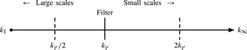
The procedure to calculate $R$ as outlined by Mathis et al. (Reference Mathis, Hutchins and Marusic2009) is followed here, but with a slight departure in the enveloping technique which is explained below. First, the velocity signal $u$ is split into large- and small-scale components using a spatial Fourier filter at a set wavenumber, arbitrarily chosen as $k_{{\it\gamma}}$ (see figure 1). We then have the large- and small-scale velocity signals $u_{L}$ and $u_{S}$ ,

(2.4) $$\begin{eqnarray}\left.\begin{array}{@{}l@{}}u_{L}={\it\alpha}_{1}\sin (k_{1}x+{\it\phi}_{1})\cdots +{\it\alpha}_{l}\sin (k_{l}x+{\it\phi}_{l})\cdots +{\it\alpha}_{{\it\gamma}-1}\sin (k_{{\it\gamma}-1}x+{\it\phi}_{{\it\gamma}-1}),\\ u_{S}={\it\alpha}_{{\it\gamma}}\sin (k_{{\it\gamma}}x+{\it\phi}_{{\it\gamma}})\cdots +{\it\alpha}_{m}\sin (k_{m}x+{\it\phi}_{m})\cdots +{\it\alpha}_{n}\sin (k_{n}x+{\it\phi}_{n})\dots \text{ to }k_{\infty }.\end{array}\right\}\end{eqnarray}$$

Here again we assume without a loss of generality that $k_{l}<k_{{\it\gamma}}<k_{m}<k_{n}$ . Next, an envelope function $\mathscr{E}(x)$ for the small-scale velocity signal is obtained using the Hilbert transform. Mathis et al. (Reference Mathis, Hutchins and Marusic2009) use the analytic signal $A$ , written as $A(x)=\sqrt{u_{S}^{2}(x)+\mathscr{ H}^{2}(x)}$ , where $\mathscr{H}(x)$ is the Hilbert transform of $u_{S}(x)$ , as an envelope of the small-scale activity. Here we take $A^{2}$ to be our envelope function, i.e. $\mathscr{E}(x)=A^{2}(x)$ . This allows for a more direct interpretation of the final result in terms of phase in triadic interactions. For the purposes of forming a correlation coefficient, as in the calculation of $R$ , $A^{2}(x)$ is a valid proxy for $A(x)$ . As $R$ is a normalized measure, no significant differences are expected in its value between the cases of $A(x)$ and $A^{2}(x)$ being used as the envelope function, and this was easily verified by experimental data (not shown here). Following the rest of the procedure, and with some trigonometric manipulation, the expression for $R$ can be reduced to the form

(2.5) $$\begin{eqnarray}R=\frac{1}{{\it\Omega}}\mathop{\sum }_{\begin{array}{@{}c@{}}\forall l,m,n\mid \\ k_{n}-k_{m}=k_{l}\\ 0<k_{l}<k_{{\it\gamma}}\\ k_{m},k_{n}>k_{{\it\gamma}}\end{array}}{\it\alpha}_{l}{\it\alpha}_{m}{\it\alpha}_{n}\sin ({\it\phi}_{l}+{\it\phi}_{m}-{\it\phi}_{n}),\end{eqnarray}$$

where ${\it\Omega}=\sqrt{\langle \mathscr{E}_{L}^{2}\rangle \langle u_{L}^{2}\rangle }$ is the normalization factor for the covariance $\langle \mathscr{E}_{L}u_{L}\rangle$ , with $\mathscr{E}_{L}$ denoting the large-scale-pass filtered envelope function. As in the case of $S$ , only triadic interactions between wavenumbers have non-zero contributions to $R$ .

Following the phase interpretation of Chung & McKeon (Reference Chung and McKeon2010), it is seen that ${\it\phi}_{l}+{\it\phi}_{m}-{\it\phi}_{n}={\rm\Delta}{\it\phi}$ in the above equation is the phase difference between the large scale $k_{l}$ and the envelope of the triadic small scales $k_{m}$ , $k_{n}$ . Hence, $R$ can be interpreted as an amplitude-weighted (and normalized) phase measure $\sin ({\rm\Delta}{\it\phi})$ of all triadic interactions where the large scale and the two triadic small scales fall on either side of the filter cutoff. It should be noticed that the skewness (2.3) is also a measure of the same phase quantity, but over all triadic interactions without any filter restrictions. The similarity between $S$ and $R$ was first pointed out by Sharma & McKeon (Reference Sharma and McKeon2013) for a single triad, i.e. a single set of three triadically consistent wavenumbers. Although $S$ and $R$ exhibit similar trends with wall-normal height in a turbulent boundary layer, it is easy to see from (2.3) and (2.5) that differences exist between the two. This is discussed in the following subsection, and an analytical relationship is established between the two phase measures.

Figure 1.

A schematic of the wavenumber line.

2.3. An exact relationship between the skewness and the amplitude modulation coefficient

There are significant differences between measured values of $S$ and $R$ in the near-wall and the outer-wake regions of a turbulent boundary layer (see for instance Mathis et al. Reference Mathis, Marusic, Hutchins and Sreenivasan2011, figure 1). These differences can be understood by a direct comparison of (2.3) and (2.5); $S$ accounts for triadic and wavenumber pair interactions over the entire wavenumber range, whereas $R$ accounts for only those triadic interactions that occur across the filter cutoff location $k_{{\it\gamma}}$ (see figure 1). Moreover, the weights and normalization factors for triadic interactions in $S$ and $R$ are different. The triadic and wavenumber pair interactions captured by $S$ but not by $R$ can be accounted for by considering the three quantities $\langle u_{S}^{3}\rangle ,\langle u_{L}^{3}\rangle ,\langle u_{L}^{2}u_{S}\rangle$ , as explained below with reference to the schematic shown in figure 1.

(i) $\langle u_{S}^{3}\rangle$ : $u_{S}$ only contains velocity scales with wavenumbers greater than $k_{{\it\gamma}}$ , hence $\langle u_{S}^{3}\rangle$ captures all triadic and wavenumber pair interactions to the right of the filter. This is similar to $\langle u^{3}\rangle$ , but $\langle u^{3}\rangle$ captures those interactions across the entire wavenumber line whereas $\langle u_{S}^{3}\rangle$ is band-limited, and likely to be most active close to the wall.

(ii) $\langle u_{L}^{3}\rangle$ : $u_{L}$ only contains velocity scales with wavenumbers smaller than $k_{{\it\gamma}}$ ; hence $\langle u_{L}^{3}\rangle$ captures triadic interactions to the left of the filter where the two smaller wavenumbers are less than $k_{{\it\gamma}}/2$ , and wavenumber pair interactions for all wavenumbers $k_{l},k_{n}$ such that $k_{n}=2k_{l}$ and $k_{1}<k_{l}<k_{{\it\gamma}}/2$ . Larger-scale activity is most prevalent in the wake region.

(iii) $\langle u_{L}^{2}u_{S}\rangle$ : with workings similar to $S$ and $R$ in (2.3) and (2.5) respectively, it can be shown that $\langle u_{L}^{2}u_{S}\rangle$ reduces to the following form:

(2.6) $$\begin{eqnarray}\langle u_{L}^{2}u_{S}\rangle =\frac{1}{2}\mathop{\sum }_{\begin{array}{@{}c@{}}\forall l,m,n\mid \\ k_{l}<k_{m}<k_{{\it\gamma}}<k_{n}\\ k_{{\it\gamma}}/2<k_{m}\\ k_{l}+k_{m}=k_{n}\end{array}}{\it\alpha}_{l}{\it\alpha}_{m}{\it\alpha}_{n}\sin ({\it\phi}_{l}+{\it\phi}_{m}-{\it\phi}_{n})+\frac{1}{4}\mathop{\sum }_{\begin{array}{@{}c@{}}l={\it\gamma}/2\\ k_{n}=2k_{l}\end{array}}^{{\it\gamma}}{\it\alpha}_{l}^{2}{\it\alpha}_{n}\sin (2{\it\phi}_{l}-{\it\phi}_{n}).\end{eqnarray}$$

The first term on the right-hand side captures triadic interactions where the intermediate wavenumber necessarily lies in between $k_{{\it\gamma}}/2$ and $k_{{\it\gamma}}$ , and the second term captures wavenumber pair interactions for all wavenumbers $k_{l},k_{n}$ such that $k_{n}=2k_{l}$ and $k_{{\it\gamma}}/2<k_{l}<k_{{\it\gamma}}$ .

From the above descriptions of $\langle u_{S}^{3}\rangle$ , $\langle u_{L}^{3}\rangle$ and $\langle u_{L}^{2}u_{S}\rangle$ , it is seen that the three quantities exactly capture the triadic and wavenumber interactions accounted for by $S$ and missed by $R$ . An analytical relationship can now be established between $S$ and $R$ . Balancing the weights between $S$ , $R$ , $\langle u_{S}^{3}\rangle$ , $\langle u_{L}^{3}\rangle$ and $\langle u_{L}^{2}u_{S}\rangle$ gives

(2.7) $$\begin{eqnarray}{\it\sigma}^{3}S=1.5{\it\Omega}R+\langle u_{S}^{3}\rangle +\langle u_{L}^{3}\rangle +3\langle u_{L}^{2}u_{S}\rangle .\end{eqnarray}$$

The terms on the right-hand side have a clear resemblance to scale-decomposed skewness, but with a scaled version of $R$ replacing $3\langle u_{L}u_{S}^{2}\rangle$ . This confirms the suggestion of Mathis et al. (Reference Mathis, Marusic, Hutchins and Sreenivasan2011) that the cross-term $3\langle u_{L}u_{S}^{2}\rangle$ can be used as an alternative or complementary diagnostic tool to $R$ .

It is worth noting that the analysis presented thus far makes no assumptions regarding the underlying dynamics of the system that generates the signal $u$ . Hence (2.7) is applicable to any statistically stationary signal in general. This helps in understanding the results of the amplitude modulation coefficient presented by Mathis et al. (Reference Mathis, Hutchins and Marusic2009) and Schlatter & Örlu (Reference Schlatter and Örlu2010) for synthetic turbulent signals. Mathis et al. (Reference Mathis, Hutchins and Marusic2009) show that $R(y)$ is nearly zero when phase information is randomly scrambled in velocity signals obtained from a turbulent boundary layer. By assigning random phases to different scales, we expect that on average the phase difference between large scales and the envelopes of two triadically interacting small scales ( ${\rm\Delta}{\it\phi}$ ) will be zero, and hence $R(y)\approx 0$ . Schlatter & Örlu (Reference Schlatter and Örlu2010) consider synthetic signals with matched probability density functions (PDFs) to real turbulent signals but with no scale (amplitude) information contained in them. However, by matching the PDF (and hence skewness), they retain the phase information contained in the real signal. Although all amplitude information is removed from the signal, as $R$ is a normalized measure, it is not surprising to see that there is a good match between $R(y)$ calculated from their real and synthetic signals.

It is seen from this analysis that both the skewness and the amplitude modulation coefficient are amplitude-weighted average measures of phase in triadic scale interactions. It should be noted that the extension of this analysis to a broader definition of triadic interactions, for example including the spanwise wavenumber and temporal frequency, is straightforward. In the following section we describe an experiment in which the natural phase relationships between scales in a turbulent boundary layer are altered by exciting a synthetic large-scale motion in the flow.

Figure 2.

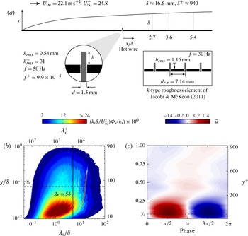
Schematic of the experimental set-up (not to scale), spectral data and synthetic mode shape. (a) The turbulent boundary layer is forced by a spatially impulsive single rib dynamic roughness, and phase-locked hot-wire measurements are made at three downstream stations as marked. Here, momentum thickness Reynolds number $Re_{{\it\theta}}=2780$ and friction Reynolds number $Re_{{\it\tau}}=940$ at the first measurement station $x=2.7{\it\delta}$ , where ${\it\delta}$ is the boundary layer thickness. The k-type roughness of Jacobi & McKeon (Reference Jacobi and McKeon2011) is shown as an inset at the bottom right of the figure for comparison. (b) Premultiplied power spectrum of streamwise velocity fluctuations at $x=2.7{\it\delta}$ (log scale in $y$ ). (c) Synthetic mode shape over one temporal period $x=2.7{\it\delta}$ (linear scale in $y$ , contour scale in $\text{m}~\text{s}^{-1}$ ).

3.1. The experiment

A zero-pressure-gradient turbulent boundary-layer flow over a smooth flat plate was set up for this study in the Merrill wind tunnel at Caltech. A spanwise-constant spatio-temporal mode was excited (or forced) in the flow following the technique of Jacobi & McKeon (Reference Jacobi and McKeon2011) with modifications. Details of the experiment were presented recently by the authors (Duvvuri & McKeon Reference Duvvuri and McKeon2014), and are recounted here in brief for the sake of completeness. Detailed description of a similar experiment can also be found in Jacobi & McKeon (Reference Jacobi and McKeon2011). Figure 2(a) shows a schematic of the flat plate and the roughness perturbation in the form of a thin rib aligned along the spanwise direction. The boundary layer with a free-stream velocity of $U_{\infty }=22.1~\text{m}~\text{s}^{-1}$ is fully turbulent with $Re_{{\it\theta}}\approx 2750$ at the perturbation rib location. The rib was oscillated sinusoidally at a frequency $f=50~\text{Hz}$ in the wall-normal direction $y$ with a peak-to-trough amplitude of $h=0.76~\text{mm}$ ( $h_{rms}=0.54\pm 0.02~\text{mm}$ ) such that the rib sat flush with the plate surface at the trough of every oscillation cycle.

The dynamic roughness perturbation introduces a dominant temporal scale and a dominant streamwise length scale (i.e. a travelling wave or a spatio-temporal mode) in the boundary layer downstream; the temporal scale corresponds to the time period of forcing ( $1/f$ ), and the length scale is a function of the roughness geometry. The k-type roughness element used by Jacobi & McKeon (Reference Jacobi and McKeon2011) is shown as an inset in figure 2 for comparison with the present study. Along with dynamic forcing effects, significant static roughness effects are reported by Jacobi & McKeon (Reference Jacobi and McKeon2011). Here, the number of roughness ribs was reduced from four to one, and the perturbation amplitude was decreased from $h_{rms}=1.16$ to 0.54 mm. With a significantly shorter streamwise extent and reduced mean blockage, any static roughness effects due to the relatively weaker perturbation at the downstream measurement locations were minimal (see the mean velocity profiles in figure 3 a). Moreover, the oscillation frequency was increased from $f=30$ to 50 Hz to generate sufficiently strong dynamic forcing effects. It is important to note at this point that multiple scales are excited by static roughness effects immediately downstream of the perturbation ( $x<1{\it\delta}$ ); this is seen in the experimental data of Jacobi & McKeon (Reference Jacobi and McKeon2011). However, these evanescent modes decay quickly and the flow is dominated by a single spatio-temporal mode for a relatively large streamwise extent.

Hot-wire measurements were made at three different stations downstream of the roughness in the canonical (no roughness perturbation, fully smooth plate) and dynamically perturbed (or forced) flows using a Dantec 55P05 boundary-layer probe ( $5~{\rm\mu}\text{m}$ diameter and 1.25 mm active length) with a Dantec StreamLine Pro anemometer.

Figure 3.

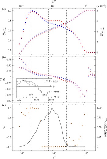
Statistical and phase data from station-1. The dashed line is the estimated critical layer location and the dash-dot lines are the locations where the synthetic mode energy drops to 15 % of its maximum value. (a) Mean streamwise velocity profiles: canonical flow (CF), ○; forced flow (FF), ▫. Variance profiles: CF, ●; FF, ▪. (b) Skewness ( $S$ ): CF, $+$ ; FF, $\times$ . Amplitude modulation coefficient ( $R$ ): CF, ▵; FF, ♢. The inset shows the difference between FF and CF for $S$ (○) and $R$ (▫). (c) Correlation coefficient ${\it\Psi}$ (●) and normalized synthetic mode energy (–).

3.2. Results: statistics, spectrum and synthetic mode shape

Data from hot-wire measurements made at the first station $x=2.7{\it\delta}$ downstream of the perturbation, herein referred to as station-1, are used for most of the analysis presented here. The boundary-layer thickness ${\it\delta}$ at station-1 based on 99 % of $U_{\infty }$ was 16.55 mm, and the momentum-thickness-based Reynolds number $Re_{{\it\theta}}$ was 2780 for the canonical flow. The friction Reynolds number $Re_{{\it\tau}}$ was estimated to be 940 using the Coles–Fernholz empirical relation, $C_{f}=2[{\it\kappa}^{-1}\log (Re_{{\it\theta}})+C]^{-2}$ ; here $C_{f}$ is the skin-friction coefficient. The relation was also used to estimate $Re_{{\it\tau}}$ for the forced flow, and wall-normal distances and streamwise wavelengths are scaled in inner units along with outer units in figures. It should be noted that the Coles–Fernholz estimate is strictly applicable only to the canonical flow; however, viscous scaling in the figures provides a useful reference. The instantaneous streamwise velocity $U(y,t)$ , where $t$ is time, is decomposed into a time mean $\overline{U}(y)$ and a fluctuating component $u(y,t)$ (Reynolds decomposition). Profiles of $\overline{U}(y)$ and variance of $u(y,t)$ at station-1 are shown in figure 3(a). The dynamic forcing effect is clearly seen in the form of an energetic bulge in the variance profile of the forced flow; this results from the excitation of a synthetic scale in the flow. As the forcing is spatially impulsive and applied only at one location, the energy associated with the synthetic scale decays with the downstream distance, and eventually the variance profile collapses onto the canonical case (see Duvvuri & McKeon Reference Duvvuri and McKeon2014, figure 2). As the mean velocity profiles of the canonical and forced flows almost overlap, there is no significant change in ${\it\delta}$ and $Re_{{\it\tau}}$ between the two flows.

Figure 2(b) shows the premultiplied power spectrum of $u$ for the forced flow at station-1 (for the corresponding spectrum of the unforced case, see Duvvuri & McKeon Reference Duvvuri and McKeon2014). Taylor’s hypothesis of frozen turbulence is used to project temporal velocity fluctuations to the streamwise spatial direction through the local mean velocity. The presence of a synthetic large scale in the forced boundary layer is distinctly seen in the spectrum of the forced flow. In a strict sense, the following analysis is valid only in the temporal domain. However, the energetic content of the synthetic mode is centred sufficiently far from the wall that any errors associated with Taylor’s hypothesis are unlikely to be sufficiently large to cause significant contamination of the results, and the conclusions presented here remain unaffected by projection from $t$ to $x$ . There is clear scale separation between the synthetic large scale and the energetic small scales that constitute the near-wall cycle of turbulence. A spatial Fourier filter is used to separate the velocity fluctuations $u$ into large and small scales ( $u=u_{L}+u_{S}$ ) for calculation of $R$ . The cutoff for the filter was chosen as ${\it\lambda}_{{\it\gamma}}=2{\rm\pi}/k_{{\it\gamma}}=5{\it\delta}$ (marked by a vertical line in figure 2 b), where the separation between the synthetic large scale and the energetic small scales is clear for all $y$ .

Following Hussain & Reynolds (Reference Hussain and Reynolds1970), the turbulent fluctuations $u(y,t)$ are further decomposed as $u(y,t)=\widetilde{u}(y)+u^{\prime }(y,t)$ into coherent and turbulent parts; here, $\widetilde{u}$ is the periodic velocity component associated with the forcing and $u^{\prime }$ is the rest of the turbulence. The periodic velocity component $\widetilde{u}(y)$ is obtained by subjecting $u(y,t)$ to a narrow-band-pass filter around the forcing frequency and then phase averaging the filter output with respect to the input forcing signal (for details, see Duvvuri & McKeon Reference Duvvuri and McKeon2014); it represents the amplitude and shape of the synthetic mode. Figure 2(c) shows $\widetilde{u}(y)$ at station-1 ( $x=2.7{\it\delta}$ ) over one temporal period. The periodic velocity component $\widetilde{u}(y)$ is also calculated at $x=3.6{\it\delta}$ and $x=5.4{\it\delta}$ (not shown here); by tracking the phase change of $\widetilde{u}(y)$ with streamwise distance (at each $x$ the local phase value of $\widetilde{u}$ is taken at the wall-normal peak), the wavelength ${\it\lambda}_{sls}$ ( $=2{\rm\pi}/k_{sls}$ ) of the synthetic mode is estimated to be $15{\it\delta}$ . The wave speed $c$ of the synthetic mode is given by $c=f{\it\lambda}_{sls}=0.59U_{\infty }$ . The critical layer location $y_{c}$ for the synthetic mode (i.e. the location in $y_{c}$ where $\overline{U}(y)=c$ ) is estimated to be $y_{c}=0.072{\it\delta}$ ( $y_{c}^{+}\approx 68$ ); this is marked by a dashed line in all relevant figures in this paper.