1 Introduction
The goal of large-eddy simulations (LES) is to accurately capture the coarse-grained dynamics of high-Reynolds-number turbulent flows (Sagaut Reference Sagaut2006). In doing so, a large majority of the turbulent kinetic energy may be resolved at a small fraction of the cost of direct numerical simulations (DNS) by replacing the fine-scale details of the flow with a subgrid scale (SGS) model for their effect on the resolved dynamics (Lilly Reference Lilly and Gladstone1967; Meneveau & Katz Reference Meneveau and Katz2000). While such an approach has, in many cases, proven successful for simulating high-Reynolds-number turbulence, many applications require a more detailed representation of the fine-scale properties of the flow. Examples include particle dispersion (Sawford Reference Sawford2001), preferential concentration of inertial particles (Maxey Reference Maxey1987; Eaton & Fessler Reference Eaton and Fessler1994), rotation and orientation dynamics of rigid particles and fibres (Pumir & Wilkinson Reference Pumir and Wilkinson2011; Chevillard & Meneveau Reference Chevillard and Meneveau2013; Voth & Soldati Reference Voth and Soldati2017), breakup and coalescence of aggregates, drops and bubbles (Maniero et al. Reference Maniero, Masbernat, Climent and Risso2012; Biferale, Meneveau & Verzicco Reference Biferale, Meneveau and Verzicco2014; Babler et al. Reference Babler, Biferale, Brandt, Feudel, Guseva, Lanotte, Marchioli, Picano, Sardina and Soldati2015; Marchioli & Soldati Reference Marchioli and Soldati2015; Spandan, Verzicco & Lohse Reference Spandan, Verzicco and Lohse2016), micro-organism motility and nutrient uptake (Batchelor Reference Batchelor1980; Karp-Boss, Boss & Jumars Reference Karp-Boss, Boss and Jumars1996; Guasto, Rusconi & Stocker Reference Guasto, Rusconi and Stocker2012), flow-induced haemolysis (Behbahani et al. Reference Behbahani, Behr, Hormes, Steinseifer, Arora, Coronado and Pasquali2009; De Tullio et al. Reference De Tullio, Nam, Pascazio, Balaras and Verzicco2012; Vitale et al. Reference Vitale, Nam, Turchetti, Behr, Raphael, Annesini and Pasquali2014; De Vita, de Tullio & Verzicco Reference De Vita, de Tullio and Verzicco2016), polymer stretching–relaxation dynamics (Balkovsky, Fouxon & Lebedev Reference Balkovsky, Fouxon and Lebedev2000; Chertkov Reference Chertkov2000; Procaccia, L’Vov & Benzi Reference Procaccia, L’Vov and Benzi2008; White & Mungal Reference White and Mungal2008), and strain-rate quenching of turbulent premixed flames (Meneveau & Poinsot Reference Meneveau and Poinsot1991; Dopazo et al. Reference Dopazo, Cifuentes, Martin and Jimenez2015).
While improvements for SGS modelling of LES have been an important topic of research for the past three decades, some focus is now shifting towards how micro-physical processes such as those mentioned above might be accurately dealt with in the context of LES, where the relevant small-scale turbulence dynamics are simply not resolved. For instance, there has been work on modelling unresolved velocity fluctuations for studying dispersion and other particle statistics such as inertial particle clustering (Kuerten & Vreman Reference Kuerten and Vreman2005; Fede, Simonin & Villedieu Reference Fede, Simonin and Villedieu2006; Mazzitelli, Toschi & Lanotte Reference Mazzitelli, Toschi and Lanotte2014; Minier, Chibbaro & Pope Reference Minier, Chibbaro and Pope2014; Ray & Collins Reference Ray and Collins2014; Park et al. Reference Park, Bassenne, Urzay and Moin2017). However, many of the aforementioned micro-physical applications are strongly affected by the gradient of the velocity field (or coarse-grained gradient depending on the scale of the physics involved), which has not received much attention in LES modelling contexts. A notable exception is the work of Chen, Jin & Zhang (Reference Chen, Jin and Zhang2016), which coupled the tensorial Ornstein–Uhlenbeck (OU) model of Pumir & Wilkinson (Reference Pumir and Wilkinson2011) to an LES of isotropic turbulence. In that case, the limitations of the OU model in faithfully representing turbulent velocity gradient dynamics severely limited the resulting accuracy. The dynamics of velocity gradients in turbulence are highly non-Gaussian (Li & Meneveau Reference Li and Meneveau2005; Wilczek & Friedrich Reference Wilczek and Friedrich2009) with significant spatio-temporal complexity. These highly non-trivial dynamics can have important consequences for a wide range of micro-physical applications where turbulence can play a role. The dynamics of velocity gradients provide not only a rich description of the local flow conditions (Meneveau Reference Meneveau2011) but are also of theoretical interest to better understand phenomena such as intermittency (Nelkin Reference Nelkin1990; Schumacher et al. Reference Schumacher, Scheel, Krasnov, Donzis, Yakhot and Sreenivasan2014) and Lagrangian chaos (Ottino Reference Ottino1989; Ott Reference Ott1993).
For sufficiently small objects and features in a turbulent environment, the flow in the immediate vicinity of a point
 $\boldsymbol{x}_{0}$
can be well approximated by a linearized description,
 $u_{i}(\boldsymbol{x},t)\approx u_{i}(\boldsymbol{x}_{0},t)+(x_{j}-x_{0,j})\unicode[STIX]{x1D608}_{ij}(\boldsymbol{x}_{0},t)$
, where
 $\unicode[STIX]{x1D608}_{ij}=\unicode[STIX]{x2202}u_{i}/\unicode[STIX]{x2202}x_{j}$
is the velocity gradient tensor having nine components. In an incompressible flow, the trace of
 $\unicode[STIX]{x1D63C}$
vanishes due to the solenoidal constraint on the velocity field, leaving eight independent quantities of interest. The velocity gradient tensor describes both the local straining and rotating behaviour of the fluid, given by the strain-rate tensor
 $\unicode[STIX]{x1D61A}_{ij}=(\unicode[STIX]{x1D608}_{ij}+\unicode[STIX]{x1D608}_{ji})/2$
and rotation-rate tensor
 $\unicode[STIX]{x1D6FA}_{ij}=(\unicode[STIX]{x1D608}_{ij}-\unicode[STIX]{x1D608}_{ji})/2$
, respectively (the rotation-rate tensor, being anti-symmetric, can be more compactly expressed by the vorticity
 $\unicode[STIX]{x1D714}_{i}=-\unicode[STIX]{x1D716}_{ijk}\unicode[STIX]{x1D6FA}_{jk}$
).
In terms of statistical descriptions of the small-scale structure of turbulence and gradients, the hypothesis of local isotropy for small-scale turbulence, which can be traced back to Kolmogorov (Reference Kolmogorov1941), i.e. ‘K41’, is very prominent and has garnered considerable empirical support (see, for example, Saddoughi & Veeravalli Reference Saddoughi and Veeravalli1994; Sreenivasan & Antonia Reference Sreenivasan and Antonia1997; Johnson et al. Reference Johnson, Hamilton, Burns and Meneveau2017). This hypothesis also provides a rationale for modelling the dynamics of small-scale quantities such as velocity gradients in the canonical flow of isotropic turbulence. The velocity gradient in isotropic turbulence, particularly from a Lagrangian perspective, has generated much interest since the work of Vieillefosse (Reference Vieillefosse1982, Reference Vieillefosse1984) and Cantwell (Reference Cantwell1992) on the restricted Euler system. The restricted Euler system shares a number of qualitative features with fully developed turbulence (not captured by an OU process) but succumbs to a finite-time singularity because important viscous and pressure effects are ignored. A simple linear damping model prevents this singularity for some but not all initial conditions (Martin, Dopazo & Valino Reference Martin, Dopazo and Valiño1998). Girimaji & Pope (Reference Girimaji and Pope1990) introduced a stochastic model with an expression for the viscous and pressure terms which by design produced a lognormal probability density function (PDF) for pseudo-dissipation. Further efforts by Jeong & Girimaji (Reference Jeong and Girimaji2003), Chevillard & Meneveau (Reference Chevillard and Meneveau2006) and Chevillard et al. (Reference Chevillard, Meneveau, Biferale and Toschi2008) borrowed a technique from tetrad modelling (Chertkov, Pumir & Shraiman Reference Chertkov, Pumir and Shraiman1999) to build a more physics-based closure using Lagrangian deformation history. Meanwhile, Wilczek & Meneveau (Reference Wilczek and Meneveau2014) computed a stochastic closure for the pressure and viscous terms in the Lagrangian velocity gradient evolution equation using Gaussian field statistics. Johnson & Meneveau (Reference Johnson and Meneveau2016) further showed that detailed analytical calculations assuming Gaussian statistics, when combined with a Lagrangian deformation map, provides a quite robust and accurate closure to model Lagrangian velocity gradients in isotropic turbulence.
In this paper, we extend the stochastic model of Johnson & Meneveau (Reference Johnson and Meneveau2016) to predict velocity gradients in inhomogeneous turbulence by coupling the model to an LES solution of the large-scale flow. The resulting model is compared with velocity gradients from DNS of a turbulent channel flow. We also demonstrate its capability to predict morphology deformation features of small droplets embedded in the channel flow. This modelling approach opens up the possibility for simulating velocity gradient effects across the wide range of natural and man-made turbulent flows for which inhomogeneity is an important feature. The structure of the paper is as follows. The relevant background is given in § 2, where the theory for the model is summarized. The details of the various numerical simulations are provided in § 3 and results are shown in § 4. A summary of results and conclusions are drawn in § 5.
2 Background and model development
This section provides background theory and modelling details for the paper. The status of energy dissipation and velocity gradients in the context of LES is reviewed in § 2.1, particularly emphasizing what small-scale information is and is not present in an LES representation of the flow. Then, § 2.2 reviews stochastic models for the velocity gradient tensor and develops the method for (one-way) coupling to LES. This coupling requires tracking the particle trajectories in LES, which is done using a modelling framework reviewed in § 2.3 along with a theoretical derivation for one of the model coefficients. Finally, to facilitate a demonstration of micro-physics which are strongly influenced by the velocity gradient, a simple model for droplet deformation and relaxation dynamics is presented in § 2.4.
In this paper, we consider the incompressible Navier–Stokes (INS) equations,
 $$\begin{eqnarray}\unicode[STIX]{x2202}_{t}u_{i}+u_{j}\unicode[STIX]{x2202}_{j}u_{i}=-\unicode[STIX]{x2202}_{i}p+\unicode[STIX]{x1D708}\unicode[STIX]{x1D735}^{2}u_{i},\quad \unicode[STIX]{x2202}_{j}u_{j}=0,\end{eqnarray}$$
for a Newtonian fluid with kinematic viscosity
 $\unicode[STIX]{x1D708}$
, where
 $u_{i}(\boldsymbol{x},t)$
is the velocity field and
 $p(\boldsymbol{x},t)$
is the pressure field (divided by density). The INS equations form the basis for the modelling and analysis of velocity gradients discussed below.
2.1 Energy dissipation and gradients in large-eddy simulations (LES)
Large-eddy simulations (LES) represent an attempt to simulate the evolution of a filtered velocity field (Germano Reference Germano1992),
 $$\begin{eqnarray}\widetilde{u}_{i}(\boldsymbol{x})=\iiint G(\boldsymbol{r};\unicode[STIX]{x1D6E5})u_{i}(\boldsymbol{x}+\boldsymbol{r})\,\text{d}^{3}r,\end{eqnarray}$$
defined using a filter kernel
 $G(\boldsymbol{r};\unicode[STIX]{x1D6E5})$
with width
 $\unicode[STIX]{x1D6E5}$
. The LES equations are derived by applying the filtering operation, (2.2), to the INS equations, (2.1),
 $$\begin{eqnarray}\unicode[STIX]{x2202}_{t}\widetilde{u}_{i}+\widetilde{u}_{j}\unicode[STIX]{x2202}_{j}\widetilde{u}_{i}=-\unicode[STIX]{x2202}_{i}\widetilde{p}+\unicode[STIX]{x1D708}\unicode[STIX]{x1D735}^{2}\widetilde{u}_{i}-\unicode[STIX]{x2202}_{j}\unicode[STIX]{x1D70E}_{ij},\end{eqnarray}$$
where
 $\unicode[STIX]{x1D70E}_{ij}=\widetilde{u_{i}u_{j}}-\widetilde{u}_{i}\widetilde{u}_{j}$
is the subgrid stress (SGS) tensor which requires a closure model (Sagaut Reference Sagaut2006). In this paper, we consider the popular, broad class of Smagorinsky models based on the eddy viscosity approximation for the deviatoric stress
 $\unicode[STIX]{x1D70E}_{ij}^{d}$
, with length scale
 $\unicode[STIX]{x1D6E5}$
and inverse time scale
 $|\widetilde{\unicode[STIX]{x1D64E}}|=\sqrt{2\widetilde{\unicode[STIX]{x1D61A}}_{ij}\widetilde{\unicode[STIX]{x1D61A}}_{ij}}$
(Smagorinsky Reference Smagorinsky1963),
 $$\begin{eqnarray}\unicode[STIX]{x1D70E}_{ij}^{d}=-2(C_{s}\unicode[STIX]{x1D6E5})^{2}|\widetilde{\unicode[STIX]{x1D64E}}|\widetilde{\unicode[STIX]{x1D61A}}_{ij},\end{eqnarray}$$
where
 $C_{s}$
is the Smagorinsky coefficient. This coefficient may be specified as a prescribed model parameter (Lilly Reference Lilly and Gladstone1967), or determined dynamically using information from the resolved flow field (Germano et al.
Reference Germano, Piomelli, Moin and Cabot1991). When considering the large-scale kinetic energy equation derived from (2.3), energy is dissipated from the filtered field in two ways: (i) resolved molecular dissipation,
 $\unicode[STIX]{x1D708}|\widetilde{\unicode[STIX]{x1D64E}}|^{2}$
, and (ii) transfer of energy to unresolved scales,
 $\unicode[STIX]{x1D6F1}=-\unicode[STIX]{x1D70E}_{ij}\widetilde{\unicode[STIX]{x1D61A}}_{ij}$
. When using a Smagorinsky model, this so-called SGS production becomes
 $\unicode[STIX]{x1D6F1}=(C_{s}\unicode[STIX]{x1D6E5})^{2}|\widetilde{\unicode[STIX]{x1D64E}}|^{3}$
, and is positive (no backscatter) as long as
 $C_{s}^{2}$
remains positive.
The goal of LES is to resolve the most energetic motions of the flow. In fact, some consider the defining quality of an LES to be the resolution of a certain percentage (e.g. 80 %) of the flow’s turbulent kinetic energy (Pope Reference Pope2000). Away from walls, this goal can often be achieved with cost relatively independent of Reynolds number since most of the energy resides in the largest decade (or so) of length scales. However, when velocity gradients are important to the application at hand, the situation becomes more difficult.
Consider a turbulent flow with Hölder exponents
 $h(\boldsymbol{x},t)$
, that is, the velocity increments at length
 $\ell$
locally scale as
 $\unicode[STIX]{x1D6FF}u(\ell )\sim \ell ^{h}$
(this scaling can also be done in a global sense for
 $L_{p}$
norms using Besov exponents (Eyink & Aluie Reference Eyink and Aluie2009)). The fully resolved velocity gradient scales as
 $|\unicode[STIX]{x1D63C}|\sim \unicode[STIX]{x1D6FF}u(\unicode[STIX]{x1D702})/\unicode[STIX]{x1D702}\sim \unicode[STIX]{x1D702}^{h-1}$
, where
 $\unicode[STIX]{x1D702}=\unicode[STIX]{x1D708}^{3/4}\langle \unicode[STIX]{x1D716}\rangle ^{-1/4}$
is the Kolmogorov length scale. Further, the filtered velocity gradient scales as
 $|\widetilde{\unicode[STIX]{x1D63C}}|\sim \unicode[STIX]{x1D6FF}u(\unicode[STIX]{x1D6E5})/\unicode[STIX]{x1D6E5}\sim \unicode[STIX]{x1D6E5}^{h-1}$
. Thus, the percentage of resolved velocity gradient can be estimated roughly as
 $$\begin{eqnarray}\frac{|\widetilde{\unicode[STIX]{x1D63C}}|}{|\unicode[STIX]{x1D63C}|}\sim \left(\frac{\unicode[STIX]{x1D702}}{\unicode[STIX]{x1D6E5}}\right)^{1-h},\end{eqnarray}$$
which becomes very small for
 $\unicode[STIX]{x1D6E5}\gg \unicode[STIX]{x1D702}$
when
 $h<1$
(
 $h\approx 1/3$
is the K41 approximation). According to (2.5), to resolve a certain fraction of the velocity gradient as the Reynolds number is increased, the grid resolution (
 ${\sim}\unicode[STIX]{x1D6E5}$
) must increase proportional to
 $\unicode[STIX]{x1D702}$
, which leads to DNS-like scaling of the computation cost. At high Reynolds numbers, direct resolution of velocity gradients becomes prohibitively expensive and further modelling effort is needed. Therefore, while the average value of the magnitude of velocity gradients in a turbulent flow can be approximated from LES according to
 $|\unicode[STIX]{x1D63C}|\sim \sqrt{\unicode[STIX]{x1D6F1}/\unicode[STIX]{x1D708}}$
, the velocity gradient’s tensorial structure, dynamical evolution, and increasing intermittency at smaller scales cannot easily be predicted in LES.
2.2 Lagrangian velocity gradients
The evolution of velocity gradients along Lagrangian paths is given by the gradient of (2.1),
 $$\begin{eqnarray}\frac{\text{d}}{\text{d}t}\unicode[STIX]{x1D608}_{ij}=-\unicode[STIX]{x1D608}_{ik}\unicode[STIX]{x1D608}_{kj}-\unicode[STIX]{x2202}_{i}\unicode[STIX]{x2202}_{j}p+\unicode[STIX]{x1D708}\unicode[STIX]{x1D735}^{2}\unicode[STIX]{x1D608}_{ij},\end{eqnarray}$$
where
 $\text{d}/(\text{d}t)=\unicode[STIX]{x2202}_{t}+u_{j}\unicode[STIX]{x2202}_{j}$
is the Lagrangian time derivative. We can consider (2.6) as a nine-component ordinary differential equation (ODE) for the velocity gradient tensor. In this view, the nonlinear
 $\unicode[STIX]{x1D63C}^{2}$
term and the isotropic part of the pressure Hessian
 $\unicode[STIX]{x1D735}^{2}p=-\text{tr}\unicode[STIX]{x1D63C}^{2}$
are represented exactly, but the deviatoric part of the pressure Hessian and the viscous Laplacian terms require closure models. A class of Lagrangian velocity gradient models have been built using the Langevin equation associated with (2.6),
 $$\begin{eqnarray}\text{d}\unicode[STIX]{x1D608}_{ij}=\left[-\unicode[STIX]{x1D608}_{ik}\unicode[STIX]{x1D608}_{kj}-\unicode[STIX]{x1D617}_{ij}+\unicode[STIX]{x1D61D}_{ij}\right]\text{d}t+\unicode[STIX]{x1D623}_{ijk\ell }\,\text{d}\unicode[STIX]{x1D61E}_{k\ell },\end{eqnarray}$$
where the stochastic forcing uses a tensorial Wiener process,
 $\langle \text{d}\unicode[STIX]{x1D61E}_{ij}\rangle =0$
and
 $\langle \text{d}\unicode[STIX]{x1D61E}_{ij}\,\text{d}\unicode[STIX]{x1D61E}_{k\ell }\rangle =\unicode[STIX]{x1D6FF}_{ik}\unicode[STIX]{x1D6FF}_{j\ell }\,\text{d}t$
. Here,
 $\unicode[STIX]{x1D617}_{ij}$
and
 $\unicode[STIX]{x1D61D}_{ij}$
represent a model for the deterministic effect of the pressure and viscous terms in (2.6), respectively. The form of (2.7) was derived by Wilczek & Meneveau (Reference Wilczek and Meneveau2014) for stochastically forced isotropic turbulence from the evolution equation for the (single-time) velocity gradient PDF, with an alternate modelling interpretation relevant to unforced turbulence discussed by Johnson & Meneveau (Reference Johnson and Meneveau2016), whereby the stochastic forcing enters as part of the model for the pressure and viscous terms accounting for interactions with nearby particle trajectories. The deterministic part of the modelled terms in (2.7),
 $P_{ij}$
and
 $V_{ij}$
, can then be constructed from conditional averages using assumptions about the statistical structure of turbulent velocity fields. The fact that the terms in (2.6) which do not require modelling (i.e. the nonlinear
 $-\unicode[STIX]{x1D63C}^{2}$
term and the isotropic part of the pressure Hessian
 $\unicode[STIX]{x1D735}^{2}p$
) give rise to a significant portion of the unique signatures of turbulent velocity gradient dynamics makes such a modelling approach quite fruitful.
In this paper, we use the Recent Deformation of Gaussian Fields (RDGF) model of Johnson & Meneveau (Reference Johnson and Meneveau2016) to prescribe the diffusion tensor
 $\unicode[STIX]{x1D623}_{ijk\ell }$
and the conditional averages in (2.7). In short, this closure approach applies a short-time deformation map
 $\unicode[STIX]{x1D60B}_{ij}^{-1}=\exp (-\unicode[STIX]{x1D63C}\unicode[STIX]{x1D70F})_{ij}$
with deformation time
 $\unicode[STIX]{x1D70F}\sim \unicode[STIX]{x1D70F}_{\unicode[STIX]{x1D702}}$
to conditional averages computed by assuming velocity fields with all
 $n$
-point PDFs being joint-Gaussian. While the Gaussian assumption makes the calculation of conditional averages tractable, the short-time deformation map introduces non-Gaussianity which is essential for the description of turbulence at small scales.
The RDGF model for the Lagrangian velocity gradients in homogeneous isotropic turbulence is
 $$\begin{eqnarray}\text{d}\unicode[STIX]{x1D608}_{ij}=\left[-\left(\unicode[STIX]{x1D608}_{ik}\unicode[STIX]{x1D608}_{kj}-\frac{\unicode[STIX]{x1D60A}_{ij}^{-1}}{\unicode[STIX]{x1D60A}_{kk}^{-1}}\text{tr}\left(\unicode[STIX]{x1D63C}^{2}\right)\right)-\left(\unicode[STIX]{x1D60E}_{ij}-\frac{\unicode[STIX]{x1D60A}_{ij}^{-1}}{\unicode[STIX]{x1D60A}_{kk}^{-1}}\text{tr}\left(\unicode[STIX]{x1D642}\right)\right)+\unicode[STIX]{x1D61D}_{ij}\right]\text{d}t+\unicode[STIX]{x1D623}_{ijk\ell }\,\text{d}\unicode[STIX]{x1D61E}_{ij},\end{eqnarray}$$
where the Gaussian calculations specify,
 $$\begin{eqnarray}\displaystyle \unicode[STIX]{x1D60E}_{ij} & = & \displaystyle \unicode[STIX]{x1D60B}_{mi}^{-1}\left[-{\textstyle \frac{2}{7}}\left(\unicode[STIX]{x1D61A}_{mk}\unicode[STIX]{x1D61A}_{kn}-{\textstyle \frac{1}{3}}\unicode[STIX]{x1D61A}_{k\ell }\unicode[STIX]{x1D61A}_{\ell k}\unicode[STIX]{x1D6FF}_{mn}\right)-{\textstyle \frac{2}{5}}\left(\unicode[STIX]{x1D6FA}_{mk}\unicode[STIX]{x1D6FA}_{kn}-{\textstyle \frac{1}{3}}\unicode[STIX]{x1D6FA}_{k\ell }\unicode[STIX]{x1D6FA}_{\ell k}\unicode[STIX]{x1D6FF}_{mn}\right)\right.\nonumber\\ \displaystyle & & \displaystyle \left.+{\textstyle \frac{86}{1365}}\left(\unicode[STIX]{x1D61A}_{mk}\unicode[STIX]{x1D6FA}_{kn}-\unicode[STIX]{x1D6FA}_{mk}\unicode[STIX]{x1D61A}_{kn}\right)\right]\unicode[STIX]{x1D60B}_{nj}^{-1},\end{eqnarray}$$
 $$\begin{eqnarray}\unicode[STIX]{x1D61D}_{ij}=-\frac{7\unicode[STIX]{x1D60A}_{kk}}{30\sqrt{15}\unicode[STIX]{x1D70F}_{\unicode[STIX]{x1D702}}}\left(\unicode[STIX]{x1D61B}_{ij}\unicode[STIX]{x1D60A}_{kk}^{-1}+2\unicode[STIX]{x1D61B}_{ik}\unicode[STIX]{x1D609}_{kj}^{-1}-\frac{4}{21}\unicode[STIX]{x1D609}_{ik}^{-1}\unicode[STIX]{x1D61A}_{kj}-\frac{2}{21}\unicode[STIX]{x1D609}_{k\ell }^{-1}\unicode[STIX]{x1D61A}_{k\ell }\unicode[STIX]{x1D6FF}_{ij}\right),\end{eqnarray}$$
where
 $\unicode[STIX]{x1D61B}_{ij}=23/105\unicode[STIX]{x1D608}_{ij}+2/105\unicode[STIX]{x1D608}_{ji}$
is a mixture of strain rate and rotation rate. The short-time deformation map is described by the inverse of the left and right Cauchy–Green tensors,
 $\unicode[STIX]{x1D60A}_{ij}^{-1}=\unicode[STIX]{x1D60B}_{ki}^{-1}\unicode[STIX]{x1D60B}_{kj}^{-1}$
and
 $\unicode[STIX]{x1D609}_{ij}^{-1}=\unicode[STIX]{x1D60B}_{ik}^{-1}\unicode[STIX]{x1D60B}_{jk}^{-1}$
, and the diffusion coefficient tensor of the stochastic forcing term is
 $$\begin{eqnarray}\unicode[STIX]{x1D623}_{ijk\ell }=-\frac{1}{3}\sqrt{\frac{D_{s}}{5}}\unicode[STIX]{x1D6FF}_{ij}\unicode[STIX]{x1D6FF}_{k\ell }+\frac{1}{2}\left(\sqrt{\frac{D_{s}}{5}}+\sqrt{\frac{D_{a}}{3}}\right)\unicode[STIX]{x1D6FF}_{ik}\unicode[STIX]{x1D6FF}_{j\ell }+\frac{1}{2}\left(\sqrt{\frac{D_{s}}{5}}-\sqrt{\frac{D_{a}}{3}}\right)\unicode[STIX]{x1D6FF}_{i\ell }\unicode[STIX]{x1D6FF}_{jk}.\end{eqnarray}$$
As derived, the RDGF model has three parameters (
 $\unicode[STIX]{x1D70F},D_{s},D_{a}$
), which are prescribed by three constraints. First, a consistency condition for the magnitude of the strain-rate tensor,
 $\langle |\unicode[STIX]{x1D64E}|^{2}\rangle =\unicode[STIX]{x1D70F}_{\unicode[STIX]{x1D702}}^{-2}$
, is required for constant energy dissipation rate. Additionally, the Betchov relations
 $\langle Q\rangle =-\langle \text{tr}[\unicode[STIX]{x1D63C}^{2}]\rangle /2=0$
and
 $\langle R\rangle =-\langle \text{tr}[\unicode[STIX]{x1D63C}^{3}]\rangle /3=0$
(Betchov Reference Betchov1956) are required for homogeneous turbulence. These three constraints fix the model parameters to
 $\unicode[STIX]{x1D70F}=0.1302\unicode[STIX]{x1D70F}_{\unicode[STIX]{x1D702}}$
,
 $D_{s}=0.1014\unicode[STIX]{x1D70F}_{\unicode[STIX]{x1D702}}^{-3}$
and
 $D_{a}=0.0505\unicode[STIX]{x1D70F}_{\unicode[STIX]{x1D702}}^{-3}$
, thus completing the specification of the RDGF model. More details concerning the development and assumptions of this model can be found in Johnson & Meneveau (Reference Johnson and Meneveau2016).
The above RDGF model was developed in the context of homogeneous isotropic turbulence. In high-Reynolds-number turbulence, the behaviour small-scale quantities such as the velocity gradient can be approximated by an assumption of local isotropy. In the present context, this means that the RDGF model for isotropic turbulence can serve as a general model for velocity gradients in inhomogeneous turbulent flows (provided we are not too close to the wall). For inhomogeneous turbulent flows, the essential information needed for using the local isotropy approximation is a local dissipation rate, which we will call
 $\hat{\unicode[STIX]{x1D716}}(\boldsymbol{x},t)$
, or equivalently, the dissipation time scale
 $\unicode[STIX]{x1D70F}_{\unicode[STIX]{x1D702}}=\sqrt{\unicode[STIX]{x1D708}/\hat{\unicode[STIX]{x1D716}}}$
for a given fluid viscosity. In theory, we can think of
 $\hat{\unicode[STIX]{x1D716}}(\boldsymbol{x},t)$
as the mean dissipation rate at a point in the flow given the entire space–time field of filtered velocity,
 $\hat{\unicode[STIX]{x1D716}}(\boldsymbol{x},t)=\langle 2\unicode[STIX]{x1D708}\unicode[STIX]{x1D61A}_{ij}\unicode[STIX]{x1D61A}_{ij}(\boldsymbol{x},t)|\widetilde{\boldsymbol{u}}\rangle$
. That is, if we simulated an ensemble of particles in the filtered flow field all at a given point
 $\boldsymbol{x}$
and time
 $t$
, their expected dissipation rate would be
 $\hat{\unicode[STIX]{x1D716}}$
.
To construct a simple model for
 $\hat{\unicode[STIX]{x1D716}}$
when LES flow information is available, it is quite natural to balance the dissipation rate from LES (
 $\unicode[STIX]{x1D6F1}$
) with this expected dissipation
 $\hat{\unicode[STIX]{x1D716}}$
for the small scales. In order to build in a cascade time delay (Meneveau & Lund Reference Meneveau and Lund1994; Wan et al.
Reference Wan, Xiao, Meneveau, Eyink and Chen2010) between production and dissipation of energy, we propose the following model,
 $$\begin{eqnarray}\frac{\text{d}\hat{\unicode[STIX]{x1D716}}}{\text{d}t}=\frac{\unicode[STIX]{x1D6F1}-\hat{\unicode[STIX]{x1D716}}}{\unicode[STIX]{x1D70F}_{\unicode[STIX]{x1D716}}},\end{eqnarray}$$
with
 $\unicode[STIX]{x1D70F}_{\unicode[STIX]{x1D716}}^{-1}=C_{\unicode[STIX]{x1D716}}\hat{\unicode[STIX]{x1D716}}^{1/3}\unicode[STIX]{x1D6E5}^{-2/3}$
being the energy cascade time lag and
 $C_{\unicode[STIX]{x1D716}}=1.5$
is seen to provide good results in § 4. At small Reynolds numbers, one can use
 $\unicode[STIX]{x1D6F1}+\unicode[STIX]{x1D708}|\widetilde{\unicode[STIX]{x1D64E}}|^{2}$
instead of just
 $\unicode[STIX]{x1D6F1}$
in (2.12) to include the resolved dissipation rate from LES as well, though this correction will be negligible at high Reynolds numbers. For this paper, given that the DNS cases used are at relatively low Reynolds numbers, we implement this correction. A model similar to (2.12) for the turbulence frequency
 $\unicode[STIX]{x1D716}/k$
was used by Sheikhi, Givi & Pope (Reference Sheikhi, Givi and Pope2009) in a filtered density function (FDF) approach to LES.
When the dissipation time scale
 $\unicode[STIX]{x1D70F}_{\unicode[STIX]{x1D702}}$
is constant in time, the RDGF model has the form,
 $$\begin{eqnarray}\frac{\text{d}}{\text{d}t}\unicode[STIX]{x1D608}_{ij}=f_{ij}(\unicode[STIX]{x1D63C}),\end{eqnarray}$$
where
 $$\begin{eqnarray}f_{ij}(\unicode[STIX]{x1D608})=-\unicode[STIX]{x1D608}_{ik}\unicode[STIX]{x1D608}_{kj}+h_{ij}(\unicode[STIX]{x1D63C})+\text{d}\unicode[STIX]{x1D60D}_{ij}/\text{d}t,\end{eqnarray}$$
and the corresponding dimensionless form,
 $$\begin{eqnarray}\frac{\text{d}}{\text{d}t^{\ast }}\unicode[STIX]{x1D608}_{ij}^{\ast }=f_{ij}^{\ast }(\unicode[STIX]{x1D63C}^{\ast }),\quad \text{where}~\unicode[STIX]{x1D608}_{ij}^{\ast }=\unicode[STIX]{x1D608}_{ij}\unicode[STIX]{x1D70F}_{\unicode[STIX]{x1D702}},~\text{d}t^{\ast }=\text{d}t/\unicode[STIX]{x1D70F}_{\unicode[STIX]{x1D702}},~f_{ij}^{\ast }=f_{ij}\unicode[STIX]{x1D70F}_{\unicode[STIX]{x1D702}}^{2}.\end{eqnarray}$$
Here,
 $h_{ij}$
represents the pressure Hessian and viscous Laplacian closures in (2.8)–(2.10). This dimensionless system is constrained to satisfy
 $\langle |\unicode[STIX]{x1D64E}^{\ast }|^{2}\rangle =1$
, as explained above for constant
 $\unicode[STIX]{x1D70F}_{\unicode[STIX]{x1D702}}$
.
When
 $\unicode[STIX]{x1D70F}_{\unicode[STIX]{x1D702}}(t)$
fluctuates in time, an added constraint term must be added to the model. This can be seen by considering the product rule to expand the dimensionless time derivative:
 $$\begin{eqnarray}\displaystyle \frac{\text{d}}{\text{d}t^{\ast }}(\unicode[STIX]{x1D608}_{ij}^{\ast })=\unicode[STIX]{x1D70F}_{\unicode[STIX]{x1D702}}\frac{\text{d}}{\text{d}t}(\unicode[STIX]{x1D608}_{ij}\unicode[STIX]{x1D70F}_{\unicode[STIX]{x1D702}})=\unicode[STIX]{x1D70F}_{\unicode[STIX]{x1D702}}^{2}\frac{\text{d}}{\text{d}t}\unicode[STIX]{x1D608}_{ij}+\unicode[STIX]{x1D608}_{ij}\unicode[STIX]{x1D70F}_{\unicode[STIX]{x1D702}}\frac{\text{d}\unicode[STIX]{x1D70F}_{\unicode[STIX]{x1D702}}}{\text{d}t}. & & \displaystyle\end{eqnarray}$$
Further, substituting for the time derivative of
 $\unicode[STIX]{x1D608}$
, it is straightforward to obtain
 $$\begin{eqnarray}f(\unicode[STIX]{x1D63C},\unicode[STIX]{x1D70F}_{\unicode[STIX]{x1D702}})=\frac{1}{\unicode[STIX]{x1D70F}_{\unicode[STIX]{x1D702}}^{2}}f^{\ast }(\unicode[STIX]{x1D63C}^{\ast })-\frac{1}{\unicode[STIX]{x1D70F}_{\unicode[STIX]{x1D702}}}\frac{\text{d}\unicode[STIX]{x1D70F}_{\unicode[STIX]{x1D702}}}{\text{d}t}\unicode[STIX]{x1D608}_{ij}.\end{eqnarray}$$
In this way, the RDGF model originally designed for constant-in-time dissipation rate can be constrained to follow any
 $\unicode[STIX]{x1D70F}_{\unicode[STIX]{x1D702}}(t)$
signal from the LES via (2.12) by adding
 $-1/\unicode[STIX]{x1D70F}_{\unicode[STIX]{x1D702}}(\text{d}\unicode[STIX]{x1D70F}_{\unicode[STIX]{x1D702}}/\text{d}t)\unicode[STIX]{x1D63C}\,\text{d}t$
to the stochastic differential equation (2.8).
2.3 Lagrangian trajectories
Lagrangian trajectories are computed by using the fluid velocity at the particle location,
 $$\begin{eqnarray}\frac{\text{d}X_{i}}{\text{d}t}=u_{i}(X_{i}(t),t)=\widetilde{u}(\boldsymbol{X},t)+u_{i}^{\prime }.\end{eqnarray}$$
In LES, however, the velocity is not fully resolved, and advancing particles using the resolved component of velocity
 $\widetilde{u}_{i}$
leads to an underprediction of dispersion. While other approaches have been developed (Ray & Collins Reference Ray and Collins2014; Park et al.
Reference Park, Bassenne, Urzay and Moin2017), in this paper we consider a stochastic model for the unresolved velocity component,
 $u_{i}^{\prime }=u_{i}-\widetilde{u}_{i}$
, by Fede et al. (Reference Fede, Simonin and Villedieu2006), which is based on the simplified Langevin model (SLM) of Pope (Reference Pope1985, Reference Pope1994),
 $$\begin{eqnarray}\text{d}u_{i}^{\prime }=\frac{\unicode[STIX]{x2202}\unicode[STIX]{x1D70E}_{ij}}{\unicode[STIX]{x2202}x_{j}}\,\text{d}t-u_{j}^{\prime }\frac{\unicode[STIX]{x2202}\widetilde{u}_{i}}{\unicode[STIX]{x2202}x_{j}}\,\text{d}t-\left(\frac{1}{2}+\frac{3}{4}C_{0}\right)\frac{\unicode[STIX]{x1D6F1}}{k_{r}}u_{i}^{\prime }\,\text{d}t+\sqrt{C_{0}\unicode[STIX]{x1D6F1}}\,\text{d}W_{i}.\end{eqnarray}$$
Here,
 $\text{d}W_{i}$
is a vector Wiener process with
 $\langle \text{d}W_{i}\rangle =0$
and
 $\langle \text{d}W_{i}\,\text{d}W_{j}\rangle =\unicode[STIX]{x1D6FF}_{ij}\,\text{d}t$
. The first term is the subscale force acting equally and opposite to its role in (2.3). The second term is a ‘production’ term for subgrid kinetic energy resulting from the subgrid velocity acting on the resolved velocity gradient. The third and fourth terms represent the SLM using
 $\unicode[STIX]{x1D6F1}=(C_{s}\unicode[STIX]{x1D6E5})^{2}|\widetilde{\unicode[STIX]{x1D64E}}|^{3}$
from the LES model as the dissipation rate. The basic form leading to (2.19) was first proposed by Gicquel et al. (Reference Gicquel, Givi, Jaberi and Pope2002) (therein called ‘VFDF2’) for the instantaneous velocity, whereas Fede et al. (Reference Fede, Simonin and Villedieu2006) rephrased it for the unresolved velocity and coupled it with an LES using a Smagorinksy–Yoshizawa subgrid model. It is worth pointing out that while we assume tracer particles for this work, generalizations for stochastic modelling of inertial particles have been considered in detail by, for example, Minier (Reference Minier2015) and reviewed by Marchioli (Reference Marchioli2017).
The third term depends on the residual (or unresolved) kinetic energy
 $k_{r}$
. To specify
 $k_{r}$
, we follow Fede et al. (Reference Fede, Simonin and Villedieu2006) and use the Yoshizawa model (Yoshizawa Reference Yoshizawa1982),
 $$\begin{eqnarray}k_{r}=2C_{y}\unicode[STIX]{x1D6E5}^{2}|\widetilde{\unicode[STIX]{x1D64E}}|^{2},\end{eqnarray}$$
where
 $C_{y}$
is the Yoshizawa constant, which results in
 $$\begin{eqnarray}\frac{\unicode[STIX]{x1D6F1}}{k_{r}}=C^{\prime }|\widetilde{\unicode[STIX]{x1D64E}}|,\end{eqnarray}$$
where
 $C^{\prime }=C_{s}^{2}/(2C_{y})$
. While
 $C_{s}$
can be computed from a dynamic procedure, for this paper we compute
 $C_{y}$
by considering a constant ratio,
 $$\begin{eqnarray}C^{\prime }=\frac{C_{s}^{2}}{2C_{y}}=\frac{1}{{\mathcal{S}}_{s}}\left(\frac{2}{3C_{k}}\right)^{3/2},\end{eqnarray}$$
where
 ${\mathcal{S}}_{s}=\langle |\widetilde{\unicode[STIX]{x1D64E}}|^{3}\rangle /\langle |\widetilde{\unicode[STIX]{x1D64E}}|^{2}\rangle ^{3/2}$
is the skewness of the resolved strain-rate magnitude and
 $C_{k}$
is the Kolmogorov constant for the energy spectrum of isotropic turbulence,
 $E(k)=C_{k}\langle \unicode[STIX]{x1D716}\rangle ^{2/3}k^{-5/3}$
. This result, with detailed derivation given in appendix A, is computed similarly to Lilly (Reference Lilly and Gladstone1967) using a spectral cutoff filter, where Lilly (Reference Lilly and Gladstone1967) assumed
 ${\mathcal{S}}_{s}=1.0$
. However, we find from the LES in this paper that
 ${\mathcal{S}}_{s}\approx 1.3$
, and so we use that value with (2.22) to obtain
 $k_{r}$
. The commonly accepted value of the Kolmogorov constant
 $C_{k}=1.6$
is used, resulting in
 $C^{\prime }\approx 0.21$
. Also, the value
 $C_{0}=2.1$
from Pope (Reference Pope1994) is used. The results of this model for dispersion in the channel flow LES are shown later, in § 4.1.
It is worthwhile mentioning that, while the RDGF stochastic model for velocity gradient is designed to describe dynamics on the viscous timescale
 $\unicode[STIX]{x1D70F}_{\unicode[STIX]{x1D702}}$
, the SLM-based model (2.19) has infinite acceleration and thus does not provide an accurate description of viscous-scale behaviour. As was pointed out in § 2.1, accurate depiction of viscous-scale behaviour is vital for the velocity gradient (or any other ‘small-scale quantity’), but this is not necessarily true for ‘large-scale quantities’ such as the velocity. For the present purposes, we consider the details of the viscous-scale velocity dynamics fairly unimportant for reproducing single-particle dispersion statistics. However, a modelling approach considering dynamics down to the viscous scale for the Lagrangian velocity could consider, for example, an acceleration-based stochastic model for the particle trajectories (Pope Reference Pope2002; Lamorgese et al.
Reference Lamorgese, Pope, Yeung and Sawford2007). Further, it should be noted that the Smagorinsky SGS model (2.4) and the SLM particle model are based on fundamentally different representations of the subgrid velocity field. An SGS model consistent with the SLM particle model would require solving the relevant transport equation for
 $\unicode[STIX]{x1D70E}_{ij}$
(Minier Reference Minier2016), which we presently avoid by following Fede et al. (Reference Fede, Simonin and Villedieu2006) and reverting to a Smagorinsky model for convenience.
2.4 Sub-Kolmogorov droplet model
As a sample application of the model to describing small-scale physics, we consider sub-Kolmogorov scale, deformable droplets sparsely distributed in a turbulent flow. Further, for our purposes here, the inertia of the droplets is neglected, assuming small Stokes number. Also, only one-way coupling is considered. Maffettone & Minale (Reference Maffettone and Minale1998) introduced a simple ellipsoidal model which describes the droplet with a symmetric morphology tensor,
 $\unicode[STIX]{x1D614}_{ij}$
. The eigenvectors of
 $\unicode[STIX]{x1D648}$
indicate the direction of the three semi-axes and (the square root of) their associated eigenvalues indicate the semi-axis lengths. The evolution of the morphology tensor includes rotation by the vorticity, deformation by the strain rate, and relaxation towards a spherical shape (
 $\unicode[STIX]{x1D614}_{ij}=\unicode[STIX]{x1D6FF}_{ij}$
),
 $$\begin{eqnarray}\frac{\text{d}\unicode[STIX]{x1D614}_{ij}}{\text{d}t}=\unicode[STIX]{x1D6FA}_{ik}\unicode[STIX]{x1D614}_{kj}-\unicode[STIX]{x1D614}_{ik}\unicode[STIX]{x1D6FA}_{kj}+f_{2}(\hat{\unicode[STIX]{x1D707}})(\unicode[STIX]{x1D61A}_{ik}\unicode[STIX]{x1D614}_{kj}-\unicode[STIX]{x1D614}_{ik}\unicode[STIX]{x1D61A}_{kj})-\frac{f_{1}(\hat{\unicode[STIX]{x1D707}})}{\unicode[STIX]{x1D70F}_{d}}\left(\unicode[STIX]{x1D614}_{ij}-\frac{3\text{III}}{\text{II}}\unicode[STIX]{x1D6FF}_{ij}\right),\end{eqnarray}$$
where
 $\text{II}$
and
 $\text{III}$
are the second and third invariants of the morphology tensor,
 $f_{1}$
and
 $f_{2}$
are modelled functions of the viscosity ratio
 $\hat{\unicode[STIX]{x1D707}}=\unicode[STIX]{x1D707}_{d}/\unicode[STIX]{x1D707}_{0}$
between droplet and surrounding fluid, and
 $\unicode[STIX]{x1D70F}_{d}=\unicode[STIX]{x1D707}_{0}R/\unicode[STIX]{x1D70E}$
is the relaxation time scale for a droplet with (undeformed) radius
 $R$
and interfacial tension
 $\unicode[STIX]{x1D70E}$
.
For this paper, we note that (2.23) can be rewritten in terms of a deformation tensor
 ${\mathcal{D}}_{ij}$
, which is related to the morphology tensor by
 $\unicode[STIX]{x1D648}=\boldsymbol{{\mathcal{D}}}\boldsymbol{{\mathcal{D}}}^{\text{T}}$
,
 $$\begin{eqnarray}\frac{\text{d}{\mathcal{D}}_{ij}}{\text{d}t}=\unicode[STIX]{x1D6FA}_{ik}{\mathcal{D}}_{kj}+f_{2}(\hat{\unicode[STIX]{x1D707}})\unicode[STIX]{x1D61A}_{ik}{\mathcal{D}}_{kj}-\frac{f_{1}(\hat{\unicode[STIX]{x1D707}})}{2\unicode[STIX]{x1D70F}_{d}}\left({\mathcal{D}}_{ij}-\frac{3\text{III}}{\text{II}}{\mathcal{D}}_{ji}^{-1}\right),\end{eqnarray}$$
where II and III are the invariants of
 $\unicode[STIX]{x1D648}$
as in (2.23). It is straightforward to show the equivalence of (2.23) and (2.24) by substituting
 $\unicode[STIX]{x1D614}_{ij}={\mathcal{D}}_{ik}{\mathcal{D}}_{jk}$
. The same information about the semi-axes can be extracted from the deformation using a singular value decomposition,
 $\boldsymbol{{\mathcal{D}}}=\unicode[STIX]{x1D650}\unicode[STIX]{x1D72E}\boldsymbol{V}^{\text{T}}$
, where
 $\unicode[STIX]{x1D650}$
is a unitary matrix comprised of the singular vectors indicating the semi-axis directions and
 $\unicode[STIX]{x1D72E}$
is a diagonal matrix whose elements are the associate singular values
 $\unicode[STIX]{x1D70E}_{1}\geqslant \unicode[STIX]{x1D70E}_{2}\geqslant \unicode[STIX]{x1D70E}_{3}$
, i.e., the length of the semi-axes (Greene & Kim Reference Greene and Kim1987). The total extent of deformation away from a spherical droplet is commonly measured using a deformation parameter,
 $D=(\unicode[STIX]{x1D70E}_{1}-\unicode[STIX]{x1D70E}_{3})/(\unicode[STIX]{x1D70E}_{1}+\unicode[STIX]{x1D70E}_{3})$
.
The viscosity ratio functions are given by (Maffettone & Minale Reference Maffettone and Minale1998),
 $$\begin{eqnarray}f_{1}(\hat{\unicode[STIX]{x1D707}})=\frac{40(\hat{\unicode[STIX]{x1D707}}+1)}{(2\hat{\unicode[STIX]{x1D707}}+3)(19\hat{\unicode[STIX]{x1D707}}+16)},\quad f_{2}(\hat{\unicode[STIX]{x1D707}})=\frac{5}{2\hat{\unicode[STIX]{x1D707}}+3}.\end{eqnarray}$$
Note that in the case of zero surface tension with unity viscosity ratio,
 $f_{2}=1$
and the fluid material deformation tensor evolution equation (Johnson & Meneveau Reference Johnson and Meneveau2015),
 $\text{d}{\mathcal{D}}_{ij}/\text{d}t=\unicode[STIX]{x1D608}_{ik}{\mathcal{D}}_{kj}$
, is recovered from (2.24), where
 ${\mathcal{D}}_{ij}=\unicode[STIX]{x2202}X_{i}/\unicode[STIX]{x2202}X_{0,j}$
, is the sensitivity of final Lagrangian position
 $\boldsymbol{X}$
to initial condition
 $\boldsymbol{X}_{0}$
. The model of Maffettone & Minale (Reference Maffettone and Minale1998), i.e. (2.23), has been successfully implemented with one-way coupling in DNS for both isotropic (Biferale et al.
Reference Biferale, Meneveau and Verzicco2014) and Taylor–Couette flows (Spandan et al.
Reference Spandan, Verzicco and Lohse2016). Here, we implement the same model in LES, but using the formulation given by (2.24).
The magnitudes of
 $\unicode[STIX]{x1D734}$
and
 $\boldsymbol{S}$
being set by the dissipation time scale, the dynamics described by (2.24) are influenced by two dimensionless parameters: the viscosity ratio already introduced and the capillary number
 $Ca$
,
 $$\begin{eqnarray}Ca=\frac{\unicode[STIX]{x1D707}_{0}R}{\unicode[STIX]{x1D70E}\unicode[STIX]{x1D70F}_{\unicode[STIX]{x1D702},bulk}},\end{eqnarray}$$
where
 $\unicode[STIX]{x1D70F}_{\unicode[STIX]{x1D702},bulk}$
is a single characteristic (or ‘bulk’) dissipation time scale of the flow, defined in the next section for a channel flow. For
 $Ca=\mathit{O}(1)$
, the deforming force of the turbulent velocity gradients fluctuates around the same magnitude as the restorative force of surface tension. The surface tension dominates when
 $Ca\ll 1$
and the particles remain very close to spherical, while for
 $Ca\gg 1$
the droplet deformation begins to be unbounded and other physical mechanisms (e.g. droplet breakup) become important. The simple ellipsoidal model used here is less accurate for highly deformed droplets near breakup (Maffettone & Minale Reference Maffettone and Minale1998). In this paper, we do not use this model to perform a detailed study of droplet behaviour in turbulence, but rather as a simple model to demonstrate the effectiveness of the velocity gradient model introduced above for evaluating the impact of turbulence on micro-physics within the flow.
Parameters for the turbulent channel flow case considered in this paper.

3 Computational set-up
3.1 Problem statement
Lagrangian particles in a turbulent channel flow at
 $Re_{\unicode[STIX]{x1D70F}}=u_{\unicode[STIX]{x1D70F}}h/\unicode[STIX]{x1D708}=1000$
are considered as a test case for the proposed modelling technique for inhomogeneous turbulent flows. The friction velocity,
 $u_{\unicode[STIX]{x1D70F}}$
, is prescribed by the imposed pressure drop, while
 $h=L_{y}/2$
is the channel half-height and
 $\unicode[STIX]{x1D708}$
is the molecular viscosity. The parameters for the particular turbulent channel flow considered here are given in table 1. The channel has unit half-height and the bulk velocity is near unity, so the unit time scale is the time to traverse a half-channel height travelling according to the mean flow rate. Under statistically stationary conditions, we consider an ensemble of particles released from random positions along the centreline of the channel (
 $y^{+}=1000$
) at
 $t=0$
. The particles disperse from the centreline according to (2.18) until
 $t=L_{t}$
while the velocity and pressure fields evolve according to (2.1). The duration of the flow,
 $L_{t}=26$
, is approximately one flow-through time in the periodic domain. The notation
 $\langle \cdot \rangle _{E}$
is used to denote Eulerian averaging (in time and homogeneous space directions
 $x$
and
 $z$
) while
 $\langle \cdot \rangle _{L}$
is used to denote averaging over the ensemble of Lagrangian trajectories which sample the flow in a biased, time-dependent manner after being released from the centreline at
 $t=0$
. As the particles disperse away from the centreline of the channel, where there is minimum dissipation rate on average, the particles tend to experience more intense velocity gradients.
In addition to velocity gradient statistics, we consider the deformation of sub-Kolmogorov scale droplets according to the simple ellipsoidal model (Maffettone & Minale Reference Maffettone and Minale1998) described in § 2.4. The droplets are initialized as spherical at
 $t=0$
and are deformed by the velocity gradient tensor according to (2.24). The ‘bulk’ dissipation time scale used here to define
 $Ca$
for the channel flow (Johnson et al.
Reference Johnson, Hamilton, Burns and Meneveau2017),
 $$\begin{eqnarray}\unicode[STIX]{x1D70F}_{\unicode[STIX]{x1D702},bulk}=\sqrt{\frac{\unicode[STIX]{x1D708}}{\langle \unicode[STIX]{x1D716}\rangle _{\mathit{space}}}}=\sqrt{\frac{\unicode[STIX]{x1D708}h}{u_{\unicode[STIX]{x1D70F}}^{2}U_{bulk}}},\end{eqnarray}$$
is constructed from the kinematic viscosity and the pumping power required to drive the flow at a volumetric rate of
 $U_{bulk}A_{\bot }$
through a cross-sectional area of
 $A_{\bot }$
. This time scale gives a single, convenient value for the average velocity gradient magnitude across the channel, although as will be shown, velocity gradient magnitudes vary significantly with distance from the wall.
Table 2 summarizes the four cases considered in this paper. A DNS dataset of turbulent channel flow from the Johns Hopkins Turbulence Databases (JHTDB) (Graham et al. Reference Graham, Kanov, Yang, Lee, Malaya, Burns, Eyink, Moser and Meneveau2016), with details given in § 3.2, is used as the baseline for judging the performance of the model. The particle trajectories and velocity gradients were calculated from the DNS data using built-in database functions (Yu et al. Reference Yu, Kanov, Perlman, Graham, Frederix, Burns, Szalay, Eyink and Meneveau2012; Kanov & Burns Reference Kanov and Burns2015; Johnson et al. Reference Johnson, Hamilton, Burns and Meneveau2017). In order to provide insight into the accuracy of the RDGF velocity gradient model isolated from LES SGS modelling accuracy concerns, an a priori case is constructed by filtering the DNS dataset (fDNS), which can be treated as a ‘perfect’ LES result. The next case consists of actually running an a posteriori LES with no input from the DNS, which can be argued to provide the most relevant results on the performance of the model in simulations. For this reason, the comparison of the a posteriori case with DNS results will be explored in the most detail. Finally, in order to highlight clearly the contribution provided by the velocity gradient modelling, it is sometimes useful to compare results with a ‘no model’ case in which the velocity gradients from the LES are used, i.e. neglecting entirely the SGS range of scales that are known to dominate the velocity gradient statistics. It should be kept in mind that the relative performance of LES velocity gradients in mimicking DNS results is sensitive to the resolution of the LES and the Reynolds number of the flow, i.e., given by the scaling arguments in § 2.1.
Methods used for calculating trajectories
 $\boldsymbol{X}$
, subgrid production
 $\unicode[STIX]{x1D6F1}$
, and velocity gradients
 $\unicode[STIX]{x1D63C}$
for the four cases considered in this paper.

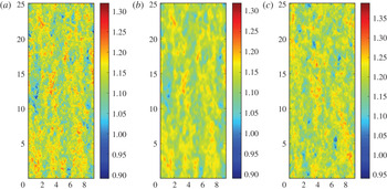
Figure 1 presents a visualization of the streamwise velocity along the centreline of the channel for the DNS, fDNS, and LES datasets. Note that the DNS and fDNS are from the same time step, so the corresponding regions of high and low velocity can be seen. The LES, of course, is from a completely different realization, so the correspondence is only qualitative with the other two. Also, as will be seen later in a more quantitative sense, the LES corresponds to a slightly smaller filter scale as compared to the fDNS. Because the mean velocity along the centreline is higher for the LES compared with DNS and fDNS, the colour scale in figure 1 has been adjusted to facilitate a qualitative visual comparison focusing on the fluctuations.
Snapshots of streamwise velocity on a plane parallel to the wall at the centre of the channel from the DNS (a), fDNS (b), LES (c). Note that the colour scale for the LES is different from the DNS and fDNS, due to the higher centreline mean velocity (see figure 3).

3.2 Direct numerical simulations
The baseline DNS data is taken from the publicly available JHTDB (Li et al.
Reference Li, Perlman, Wan, Yang, Meneveau, Burns, Chen, Szalay and Eyink2008). The channel flow dataset from Graham et al. (Reference Graham, Kanov, Yang, Lee, Malaya, Burns, Eyink, Moser and Meneveau2016) stores velocity and pressure at each grid location every five simulation time steps for one flow-through time, which amounts to 24 GB per snapshot and requires nearly 100 TB for the 4000 snapshots saved (not including overhead). This dataset was produced using the simulation code of Lee, Malaya & Moser (Reference Lee, Malaya and Moser2013), which uses pseudo-spectral discretization with
 $2/3$
-rule dealiasing (Orszag Reference Orszag1971) in the streamwise (
 $x$
) and spanwise (
 $z$
) directions. In the wall-normal (
 $y$
) direction, a collocation method using seventh-order B-splines is employed. The Navier–Stokes equations, (2.1), were solved in wall-normal velocity–vorticity form, and the pressure Poisson equation was solved only when needed for storage on the database, i.e., every 5 time steps. Time advancement was done with a third-order low-storage Runge–Kutta scheme. The parameters for the simulation are given in table 1 and the details of the numerical discretization are given in table 3. The numerical resolution in terms of effective Kolmogorov scale
 $\unicode[STIX]{x1D702}(y)=\sqrt{\unicode[STIX]{x1D708}/\langle \unicode[STIX]{x1D716}|y\rangle _{E}}$
remains near
 $k_{max}\unicode[STIX]{x1D702}\sim 1$
which, while typical for isotropic simulations, may not be sufficiently fine for capturing the most extreme velocity gradient events in the flow (Donzis, Yeung & Sreenivasan Reference Donzis, Yeung and Sreenivasan2008).
The DNS particle trajectories for the baseline and a priori cases were tracked through the database using the built-in getPosition function. This function solves (2.18) using a second-order predictor–corrector method with sixth-order Lagrange interpolation for the velocity at the particle location (fourth- and eighth-order interpolation is also available). For more details on the parallel implementation of the particle tracking in the database, see Kanov & Burns (Reference Kanov and Burns2015), Johnson et al. (Reference Johnson, Hamilton, Burns and Meneveau2017). Similarly, the velocity gradients at the particle locations were computed from the database using the built-in getVelocityGradient function with fourth-order finite differencing and fourth-order Lagrange interpolation.
For the a priori test case, every sixteenth snapshot was downloaded and filtered using a non-isotropic box filter. The box filter was implemented by averaging over 32 grid points with trapezoidal rule integration in each direction and storing the value on a new grid point at the centroid of the averaged region. The filtered DNS (fDNS) dataset is computed for every sixteenth grid point, so that there is a factor of two overlap between neighbouring points on the filtered grid. In this way, the grid for the fDNS is also non-uniform in the wall-normal direction with
 $y^{+}\approx 8$
for the first grid point away from the wall. It should be noted that such a grid would not be optimal for an actual LES simulation since the boundary conditions would be difficult to set, but is unproblematic for present purposes. The numerical details of the fDNS dataset are given in table 3.
Mean velocity (a) and Reynolds stress tensor components (b) profiles for DNS (continuous lines) and filtered DNS (symbols). In (a), the well-established linear,
 $\langle u^{+}\rangle =y^{+}$
(dotted line), and log-law,
 $\langle u^{+}\rangle =\ln y^{+}/0.41+5.2$
(dashed line), profiles are also shown for reference. For the Reynolds stress components in (b):
 $\langle {u^{\prime }}^{2}\rangle _{E}$
(◯),
 $\langle {v^{\prime }}^{2}\rangle _{E}$
(▿),
 $\langle {w^{\prime }}^{2}\rangle _{E}$
(▵), and
 $\langle u^{\prime }v^{\prime }\rangle _{E}$
(▫).

Parameters for the DNS, filtered DNS, and LES databases used in this paper.

The results for Eulerian-averaged velocity profile and Reynolds stress components for the DNS and fDNS datasets are shown in figure 2. The mean velocity profile displays the expected log-law behaviour
 $\langle u\rangle ^{+}\approx (1/\unicode[STIX]{x1D705})\ln \left(y^{+}\right)+B$
with
 $\unicode[STIX]{x1D705}\approx 0.41$
and
 $B\approx 5.2$
. The filtered dataset matches this mean velocity profile well except for the first two grid points in the buffer region, where spatial smoothing in the wall-normal direction causes the mismatch. The velocity variances, however, are significantly impacted by the filtering procedure, and roughly half of the turbulent kinetic energy is unresolved.
In the first fDNS tests, trajectories computed from the fully resolved DNS dataset are used for the a priori test so as to avoid introducing errors from the subgrid dispersion model of § 2.3. Care is also taken in establishing dissipation rates from the fDNS so as to match DNS dissipation rates in the sense of the mean profile
 $\langle \unicode[STIX]{x1D716}|y\rangle _{E}$
. The details of the fDNS dissipation rate are given in appendix B. Using DNS information to carefully construct the fDNS data allows the a priori case to focus on the particular errors of the RDGF model without introducing other modelling errors involved in coarse-grained simulations. The LES simulation described next then provides an a posteriori view on the model’s effectiveness in the context of other modelling errors such as particle trajectory errors and LES SGS model errors.
3.3 Large-eddy simulation
A wall-modelled large-eddy simulation of the same turbulent channel flow provides the main (a posteriori) test case for the velocity gradient model. As with the DNS simulation, the parameters of the LES are given in table 1. The in-house LESGO code (LESGO: A parallel pseudo-spectral large-eddy simulation code. https://lesgo-jhu.github.io/lesgo (2017)) was used to generate a dataset with a time sequence of snapshots mimicking those from the fDNS. This code uses pseudo-spectral treatment with
 $2/3$
dealiasing in the wall-parallel directions and second-order finite differencing on a staggered grid in the wall-normal direction. The wall-normal grid spacing is constrained to be uniform. With 32 grid points across the channel,
 $\unicode[STIX]{x1D6E5}y^{+}=62.5$
, and the first grid point for wall-parallel velocity components resides at
 $y^{+}=31.25$
, at the inner edge of the log-law region. The equilibrium specification of Moeng (Reference Moeng1984) is used to set the boundary condition at the wall along with a no-penetration condition. Time is advanced with a second-order Adams–Bashforth method and the pressure Poisson equation is used to maintain a solenoidal velocity field to within machine precision. The scale-dependent Lagrangian dynamic Smagorinsky model (Bou-Zeid, Meneveau & Parlange Reference Bou-Zeid, Meneveau and Parlange2005) is used for the subgrid stresses. This model is also used to compute
 $\unicode[STIX]{x1D6F1}=(C_{s}\unicode[STIX]{x1D6E5})^{2}|\widetilde{\unicode[STIX]{x1D64E}}|^{3}$
for input to (2.12) to determine the dissipation rate for the velocity gradient model. While the LES resides on a grid having the same dimensions as the fDNS in wall-normal planes, the wall-normal spacing is different (uniform versus non-uniform) and the filter width is chosen using the grid spacing (rather than twice the grid spacing as in the fDNS case). The result is that the LES results are more finely resolved than the fDNS, as is apparent in figure 1. The numerical details of the LES dataset are given in table 3.
The LES results provide quite accurate mean velocity and Reynolds stress profiles, as shown in figure 3. The first few grid points show excellent agreement with the DNS log-law. The wake region correction, however, appears to be overpredicted, which leads to the overprediction of bulk velocity (flow rate) seen in table 3, i.e., an underprediction of the friction coefficient. The overprediction of bulk velocity at a prescribed pressure drop leads to an overprediction of volume-averaged dissipation rate (pumping power), and hence a slight underprediction of
 $\unicode[STIX]{x1D70F}_{\unicode[STIX]{x1D702},bulk}$
. The majority of the turbulent kinetic energy is resolved by the LES, in keeping with general heuristics for LES resolution (Pope Reference Pope2000), which highlights the smaller effective filter width in the LES results compared with fDNS in § 3.2.
Mean velocity (a) and Reynolds stress tensor components (b) profiles for DNS (continuous lines) and LES (symbols). In (a), the well-established linear,
 $\langle u^{+}\rangle =y^{+}$
(dotted line), and log-law,
 $\langle u^{+}\rangle =\ln y^{+}/0.41+5.2$
(dashed line), profiles are also shown for reference. For the Reynolds stress components in (b):
 $\langle {u^{\prime }}^{2}\rangle$
(◯),
 $\langle {v^{\prime }}^{2}\rangle$
(▿),
 $\langle {w^{\prime }}^{2}\rangle$
(▵), and
 $\langle u^{\prime }v^{\prime }\rangle$
(▫).

Of even more relevance to the modelling effort at hand is the prediction of wall-normal dependence of dissipation rates. For the LES, we do not allow for any use of information from the DNS. The dissipation rate in the LES is determined by adding the resolved dissipation rate
 $\unicode[STIX]{x1D708}|\widetilde{\unicode[STIX]{x1D64E}}|^{2}$
to the subgrid production rate
 $\unicode[STIX]{x1D6F1}$
. The resulting Kolmogorov scale as a function wall distance is shown in figure 4(a) compared with DNS. Overall, the prediction is quite acceptable, although there is a noticeable overprediction of dissipation rate throughout most of the channel (the equilibrium model underpredicts the dissipation in the near-wall region, but as shown in table 3, the volume-averaged dissipation is overpredicted). To provide some perspective to the level of differences between LES and DNS, figure 4(a) shows the Kolmogorov scale using only the resolved dissipation rate (i.e. if no model for unresolved velocity gradients is used). A significant error is committed in this case because velocity gradients are dominated by the smallest scales, which are unresolved in the LES even when most of the velocity fluctuations are resolved. This error in velocity gradient magnitude will only increase with increasing Reynolds number, as discussed in § 2.1. In figure 4(b), the average Smagorinsky coefficient determined in the LES is shown against the assumed Smagorinsky coefficient used for the fDNS in § 3.2. While the turbulence is more finely resolved in the LES compared to the fDNS, the Smagorinsky coefficient is also quite different between the two cases, since
 $C_{s}$
can also depend on resolution, type of filtering, etc.
(a) Kolmogorov time scales
 $\unicode[STIX]{x1D70F}_{\unicode[STIX]{x1D702}}=\sqrt{\unicode[STIX]{x1D708}/\langle \unicode[STIX]{x1D716}|y\rangle _{E}}$
from DNS (——), LES-RDGF (◯), and LES-NM (▵). (b) Smagorinsky coefficient prescribed for fDNS-RDGF (——), i.e. (B 1), and
 $\langle C_{s}|y\rangle _{E}$
as computed by the LES with the scale-dependent Lagrangian dynamic formulation (◯).

3.4 Stochastic differential equations
For each case enumerated in table 2, an ensemble of 172 800 particles is initialized on the centreline of the channel with location in
 $x$
and
 $z$
determined in the following way. The domain in
 $x$
and
 $z$
is split into
 $24\times 9$
square regions of size
 $\unicode[STIX]{x03C0}/3\times \unicode[STIX]{x03C0}/3$
and the particles are divided evenly into 800 per subdomain. Each particle is given a random
 $x$
and
 $z$
location within its subdomain from a uniform distribution. While the baseline and a priori cases use the built-in interpolation, differentiation, and particle advancement from the JHTDB database, the a posteriori and no-model cases use second-order finite differencing, trilinear interpolation, and a second-order predictor–corrector time advancement. The particles are advanced in the LES using the resolved velocity plus the stochastic model for the unresolved velocity, (2.19), which itself is updated with a second-order predictor–corrector method for stochastic differential equations (Honeycutt Reference Honeycutt1992). The same predictor–corrector method is used to update (2.8) for the velocity gradients and (2.24) for the droplet morphologies. Note that the diffusion coefficients in the stochastic differential equations (2.8) and (2.19) do not depend on any of the stochastic variables, so the remarks of Minier, Cao & Pope (Reference Minier, Cao and Pope2003) do not apply concerning the consistency of the predictor–corrector scheme.
The stochastic differential equations (SDE) for velocity and velocity gradient are initialized by starting with a random Gaussian condition and running the stochastic model for each particle frozen at its initial location for a start-up time until transients subside. Then that result is used to initialize the velocity and velocity gradient in the particle dispersion simulation. The droplet morphology tensors are initialized to the identity tensor (indicating a spherical droplet). When the particles travel below the first grid point in the LES (
 $y^{+}<31.25$
) the velocity gradient model is turned off and arbitrarily set to
 $\unicode[STIX]{x1D608}_{ij}=0$
because the LES flow is no longer resolved below this point and an equilibrium wall model is used. Accordingly, when statistics are taken over the ensemble of particles, those closer to the wall than
 $y^{+}=100$
are not included in the ensemble, since particles below this threshold will experience velocity gradient stretching statistics which differ significantly from isotropic turbulence (Johnson et al.
Reference Johnson, Hamilton, Burns and Meneveau2017). This approach focuses the comparisons on the region of the channel flow displaying isotropic turbulence-like velocity gradient statistics, i.e., where the model assumptions are expected to hold. The discrepancy between the model cutoff at
 $y^{+}=31.25$
and the post-processing observation cutoff at
 $y^{+}=100$
provides a safeguard against the propagation of modelling errors from
 $y^{+}<31.25$
into the observed results as particles move towards and away from the wall in time. It is also worthwhile to note that the SLM particle model used here also would require modification to be accurate in the near-wall region, such as those introduced by Dreeben & Pope (Reference Dreeben and Pope1998), Waclawczyk, Pozorski & Minier (Reference Waclawczyk, Pozorski and Minier2004).
Finally, for the droplet deformation, it is possible for regions of strong velocity gradient for high-
 $Ca$
droplet to undergo unbounded deformation. In that case, numerical round-off errors become more significant when the disparity between singular values (ellipsoid semi-axes) becomes large. To prevent this, droplets with
 $D>0.9999$
at any time step are removed from the ensemble at the time step and are not replaced.
4 Results
In this section, the results for particle trajectories (§ 4.1), velocity gradients (§ 4.2), and droplet deformation (§ 4.3) are shown. We primarily focus on the comparison of the LES-RDGF results with DNS, although the other cases in table 2 are used at times to shed further light on the accuracy of the various models used. Figure 5 shows sample time histories for wall-normal location, transverse velocity gradient, and droplet deformation for six trajectories chosen at random. As the particles approach closer to the boundaries of the channel at
 $y=-1$
and
 $y=1$
, they tend to experience higher velocity gradient magnitudes which fluctuate at higher frequencies.
Sample time histories of particle locations in three dimensions (a), the wall-normal location (b,c), the transverse velocity gradient (d,e) and deformation magnitude parameter
 $D$
(f,g) from the DNS (b,d,f) and LES-RDGF (c,e,g) results for 6 independent Lagrangian trajectories. The droplets shown are have
 $Ca=1.0$
and
 $\hat{\unicode[STIX]{x1D707}}=1.0$
.

4.1 Particle dispersion statistics
It is important to first validate the dispersion of particles in LES away from the centreline by the combination of resolved velocity and the stochastic model for subgrid velocity contributions, § 2.3. Such a validation is presented in figure 6 by comparing particle location PDFs as a function of time from the LES and DNS cases. The distributions of particles at eight different times are shown, four early times in panel (a) (
 $0.26\leqslant t\leqslant 2.34$
) and four later times in panel (b) (
 $2.6\leqslant t\leqslant 23.4$
). The LES with the stochastic model provides excellent agreement with the dispersion seen in the DNS, with some small differences arising at later times. The first particles begin to interact with the wall around
 $t\approx 10$
. After that, there is a small but noticeable underprediction of the uniformity of the particle location PDF given by the LES results. The overall results are, however, quite good.
Distribution of particles at different times after being released from the centreline at
 $t=0$
. Continuous lines show the distributions from DNS while symbols show the results from LES with stochastic model for subgrid velocity. (a)
 $t=0.26$
(▫),
 $t=0.78$
(◯),
 $t=1.56$
(▵),
 $t=2.34$
(▿). (b)
 $t=2.6$
(▫),
 $t=7.8$
(◯),
 $t=15.6$
(▵),
 $t=23.4$
(▿).

4.2 Velocity gradient statistics
We now compare the results of the LES-RDGF model with DNS results in terms of the magnitude and tensorial structure of the velocity gradient along particle paths. The magnitude of velocity gradient determines the dissipation rate and thus establishes the ability of turbulence to rotate, deform, and otherwise affect small objects in a flow. Meanwhile, the statistical topology of velocity gradients are also important for accurately capturing how various micro-physical parameters, such as the aspect ratio of rigid particles in Jeffery’s equation (Jeffery Reference Jeffery1922; Junk & Illner Reference Junk and Illner2007) or the capillary number of small droplets in (2.24), impact the efficiency of velocity gradients in imposing their effects. Following a presentation of results for general velocity gradient statistics, we pursue further validation for the particular case of small droplets in § 4.3.
Figure 7 considers the distribution of dissipation and enstrophy (
 $\unicode[STIX]{x1D712}=(1/2)\unicode[STIX]{x1D714}_{i}\unicode[STIX]{x1D714}_{i}$
), characterizing the fluctuations in velocity gradient magnitudes in the flow. These distributions are computed by averaging over the particle ensembles and averaging in time. As a result, these PDFs contain both internal fluctuations of the RDGF velocity gradient model, as well as fluctuations due to the spatial–temporal behaviour of
 $\unicode[STIX]{x1D6F1}$
from LES. In this figure, the results of the a posteriori case compare quite favourably with the DNS results, indicating the accuracy of the fluctuations within the RDGF model which generate stretched-exponential tails in the dissipation and enstrophy PDFs. The dotted lines in this figure indicate the distribution of resolved dissipation rate in the LES (i.e., the ‘no model’ case), which severely underpredicts the intermittency of dissipation and enstrophy – in addition to significantly underpredicting the mean dissipation. Thus, figure 7 highlights the importance of the subgrid velocity gradient model in generating accurate intermittency levels for extreme fluctuations in the velocity gradient magnitude.
Probability distribution functions for dissipation (a) and enstrophy (b) using an ensemble of all particle locations at each time for
 $0<t<L_{t}$
, excluding
 $y^{+}<100$
. The continuous black line indicates LES-RDGF results compared with DNS (red dashed line) and LES-NM results (black dotted line).

Turbulence dynamics is known to generate a non-trivial signature in the structure of the velocity gradient tensor. For instance, the vorticity vector tends to align most prevalently with the strain-rate eigenvector associated with its intermediate eigenvalue,
 $\unicode[STIX]{x1D6EC}_{2}$
, while noticeably avoiding alignment with the compressive eigenvector with eigenvalue
 $\unicode[STIX]{x1D6EC}_{3}<0$
(Ashurst et al.
Reference Ashurst, Kerstein, Kerr and Gibson1987). The RDGF model, by faithfully capturing the nonlinear self-stretching term in the governing equations, has been shown to capture this tendency well (Johnson & Meneveau Reference Johnson and Meneveau2016). Indeed, the results for this alignment tendency are quite accurate in LES-RDGF, as shown in figure 8(a). Without using any model for unresolved velocity gradients, the LES particularly underpredicts the tendency of vorticity to align perpendicularly with the
 $\unicode[STIX]{x1D6EC}_{3}$
eigenvector. Additionally, the
 $s^{\ast }$
parameter, introduced by Lund & Rogers (Reference Lund and Rogers1994) for quantifying the tendency of the strain-rate tensor to deform spherical material elements towards prolate (
 $s^{\ast }<0$
) or oblate (
 $s^{\ast }>0$
) ellipsoids, has its own unique signature in turbulence. Shown in figure 8(b), the PDF of
 $s^{\ast }$
is also predicted quite successfully by the LES-RDGF model, while the LES-NM results underpredict the bias towards oblate topologies. The coarse-grained velocity gradient evolution equations share the same self-stretching term with the fully resolved equation; therefore, the results in figure 8 for LES-NM are qualitatively the same as DNS.
Probability distribution functions for alignment cosine between vorticity and strain-rate eigenvectors (a) and topology indicator
 $s^{\ast }=-3\sqrt{6}\unicode[STIX]{x1D6EC}_{1}\unicode[STIX]{x1D6EC}_{2}\unicode[STIX]{x1D6EC}_{3}/(\unicode[STIX]{x1D6EC}_{1}^{2}+\unicode[STIX]{x1D6EC}_{2}^{2}+\unicode[STIX]{x1D6EC}_{3}^{2})^{3/2}$
(b) using an ensemble of all particle locations at each time for
 $0<t<L_{t}$
, excluding
 $y^{+}<100$
. The continuous lines indicate LES-RDGF results compared with DNS (dashed lines) and LES-NM results (dotted lines). In (a), colours indicate the eigenvectors associated with largest eigenvalue (blue), intermediate eigenvalue (green), smallest eigenvalue (red).

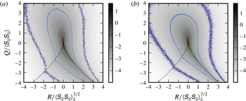
Finally, in figure 9, the joint-PDF of invariants
 $Q=-\text{tr}\unicode[STIX]{x1D63C}^{2}/2$
and
 $R=-\text{tr}(\unicode[STIX]{x1D63C}^{3})/3$
are considered from the DNS and the LES-RDGF results. It is well known that turbulence dynamics generates a signature feature in this joint-PDF, namely, the increased probability for rare fluctuations along the right-hand side of the so-called Vieillefosse tail in the fourth quadrant. This feature is intimately connected with the nonlinear dynamics of the
 $\unicode[STIX]{x1D63C}^{2}$
term in (2.6), and hence is naturally captured in the RDGF and other similar models (Chevillard et al.
Reference Chevillard, Meneveau, Biferale and Toschi2008; Wilczek & Meneveau Reference Wilczek and Meneveau2014; Johnson & Meneveau Reference Johnson and Meneveau2016). Figure 9 highlights the accuracy of the RDGF model in reproducing the key features of the PDF in
 $QR$
invariant space.
Logarithmically spaced contours of the joint probability density function for the second and third invariants of the velocity gradient tensor along the particle trajectories, excluding
 $y^{+}<100$
. The results of DNS (a) are compared with LES-RDGF model results (b).

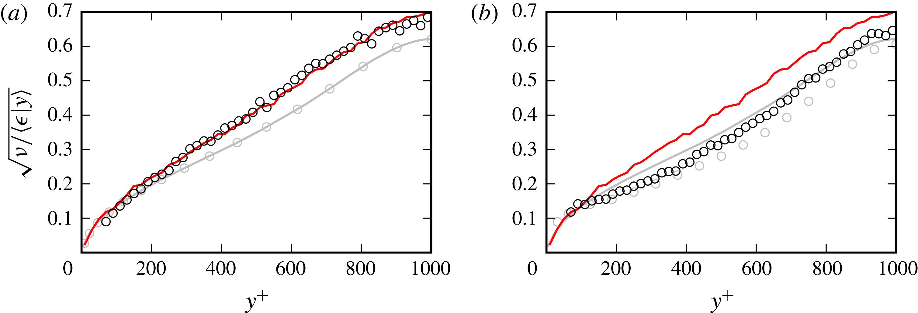
The discussion of velocity gradient accuracy in this section so far has centred on the benefits of the stochastic model, namely, the tensorial structure and intermittent fluctuations of the velocity gradient. We now turn our attention to predictions of the mean dissipation rates (velocity gradient magnitudes). As will be seen, inherent difficulties exist for providing accurate inputs to the RDGF model (i.e. accurate trajectory-specific dissipation rates) from the LES. The ensemble of Lagrangian particles is initialized at the centre of the channel, where there is a minimum of dissipation rate from an Eulerian perspective. However, as illustrated by the DNS results in figure 10, the average dissipation rate over the whole ensemble initially decreases (i.e., the dissipation time scale increases), even as the particles spread to locations nearer the wall where there is more dissipation in terms of Eulerian averages. Furthermore, in figure 11, it can be seen from DNS by comparing the red and grey continuous lines (or from the model comparing black and grey circles), that Lagrangian particles which begin in the centreline tend to sample regions with lower dissipation than given by Eulerian averaging.
Kolmogorov time scale
 $\unicode[STIX]{x1D70F}_{\unicode[STIX]{x1D702}}=\sqrt{\unicode[STIX]{x1D708}/\langle \unicode[STIX]{x1D716}\rangle _{L}}$
with averaging over the particle ensemble as a function of time after release from the centreline. The DNS results (dashed red) are compared with fDNS-RDGF (continuous grey) and LES-RDGF (continuous black).

Kolmogorov time scales as a function of wall distance for Eulerian averaging (grey) and particle ensemble averaging at time
 $t=23.4$
(black). Continuous lines indicate DNS results and symbols (◯) indicate RDGF results. (a) fDNS-RDGF (a priori) compared with DNS. (b) LES-RDGF (a posteriori) compared with DNS.
This effect can be understood as follows. While it is true that Eulerian-averaged dissipation is minimum at the centre of the channel, a more extreme minimum at the centreline is found in the SGS production results (see figure 18). In fact, from a Reynolds-averaged Navier–Stokes (RANS) perspective, the production of turbulent kinetic energy from mean flow energy is exactly zero (by symmetry) at the centreline. The following picture emerges as a simplification of the physics. While no kinetic energy is produced at the centreline, as the energy cascade proceeds to small scales, turbulent diffusion tends to move turbulent energy from high-production regions nearer to the wall towards the centreline, resulting in a more uniform profile for large-scale energy dissipation as the filter width is decreased. Still, even at the smallest scales (i.e. viscous dissipation in unfiltered equations), the profile of dissipation rate is not perfectly uniform.
Some evidence has been shown in isotropic turbulence that the energy cascade has a distinct Lagrangian characteristic (Meneveau & Lund Reference Meneveau and Lund1994; Wan et al.
Reference Wan, Xiao, Meneveau, Eyink and Chen2010), and that fluctuations in SGS production are correlated with molecular dissipation fluctuations with a time lag along Lagrangian trajectories, an effect which motivates the use of (2.12). This suggests that while particles starting on the centreline tend to have the least dissipation rate compared to starting elsewhere, at a slightly later time, their dissipation rate is strongly affected by their SGS production rate from when they were on the centreline. The initial phase of increasing dissipation time scale in figure 10 suggests that this Lagrangian cascade effect is, at least initially, stronger than the effect of particle dispersion to higher dissipation regions (in an Eulerian-averaged sense) nearer the wall. As the particle ensemble continues to spread towards the walls and the memory of initial conditions continues to fade, the average dissipation rate over the particle ensemble increases as expected from the Eulerian observations. However, as shown by figure 11, this Lagrangian effect can still be seen even at much later times by conditional averaging based on
 $y$
.
In the a priori test case, shown as a grey line in figure 10, the actual DNS trajectories are used and a non-equilibrium correction (explained in appendix B) ensures an accurate wall-normal profile of Eulerian-averaged dissipation rates in the fDNS. The result is that this initial ‘bump’ in the ensemble time scale is captured and the time history of particle ensemble dissipation rate is quite accurately reproduced. In fact, the time lag model between
 $\unicode[STIX]{x1D6F1}$
and
 $\hat{\unicode[STIX]{x1D716}}$
given in (2.12) has been introduced and the coefficient
 $C_{\unicode[STIX]{x1D716}}=1.5$
has been chosen precisely to accurately capture this effect, which can be important in non-homogeneous flows. Similarly, figure 11 shows that dissipation rates conditioned on wall distance are also captured well in the a priori case due the combination of accurate Eulerian-averaged dissipation profiles and Lagrangian trajectories. However, the results for the a posteriori test case are not as accurate, owing both to a deterioration in accuracy of the trajectories themselves due to the limitations of the stochastic dispersion model described in § 2.3 and to the overprediction of Eulerian-averaged dissipation rate by the LES, as shown in figure 4. These errors are largely independent of the details of the RDGF velocity gradient model, and improvements in velocity gradient magnitude would need to be accomplished primarily through a more accurate model for
 $\hat{\unicode[STIX]{x1D716}}$
in the LES, for example, by including turbulent diffusion effects in the spirit of RANS modelling of the
 $\unicode[STIX]{x1D716}$
equation (Pope Reference Pope2000; Wilcox Reference Wilcox2006). Improved accuracy of subgrid dispersion modelling could also be helpful here. It is important to recall from figure 4, and more generally from the scaling arguments of § 2.2, that the LES with no model will more severely underpredict the dissipation rates, and the LES-RDGF model still represents a significant improvement which is even more important as Reynolds number increases, as emphasized in § 2.2.
The results shown in this section (and the following one) have neglected data from any particle closer to the wall than 100 viscous units, so as to compare only data from regions which roughly follow local isotropy behaviour at small scales in this flow (Johnson et al. Reference Johnson, Hamilton, Burns and Meneveau2017). A clear limitation to the LES-RDGF model as presented here is that the RDGF model is designed for isotropic (or approximately isotropic) turbulence at small scales. Near the wall, this type of behaviour is no longer seen, and capturing velocity gradient statistics in the near-wall region (as well as at higher Reynolds number flows) will require more detailed future modelling efforts.
4.3 Droplet deformation statistics
To illustrate the benefits and predictive properties of the velocity gradient modelling technique proposed in this paper, we choose one particular application for which velocity gradient information is necessary, namely predicting deformation statistics of sub-Kolmogorov scale droplets. The droplets are evolved numerically according to (2.24) using a second-order predictor–corrector method. They are deformed by the velocity gradients from the stochastic model (one-way coupling). The main parameter used to quantify the magnitude of deformation for a droplet is
 $$\begin{eqnarray}D=\frac{\unicode[STIX]{x1D70E}_{1}-\unicode[STIX]{x1D70E}_{3}}{\unicode[STIX]{x1D70E}_{1}+\unicode[STIX]{x1D70E}_{3}},\end{eqnarray}$$
where
 $\unicode[STIX]{x1D70E}_{i}$
is the
 $i$
th singular value of the deformation tensor
 $\boldsymbol{{\mathcal{D}}}$
. These three singular values, representing the lengths of the three semi-axes of the ellipsoid, are computed using a singular value decomposition routine from LAPACK. The deformation parameter
 $0\leqslant D<1$
takes on the value
 $D=0$
when the droplet is spherical (as in the initial condition) and asymptotically approaches
 $D=1$
for strongly deformed droplets (
 $\unicode[STIX]{x1D70E}_{1}\gg \unicode[STIX]{x1D70E}_{3}$
). In this way, the temporal history of
 $D$
(and other droplet measures) is computed along each trajectory.
For
 $Ca=1$
, figure 12 compares the PDF of
 $D$
for the ensemble of droplets at a time late in the simulation. It is clear that the LES-NM results significantly underpredict the extent of deformation, which is a straightforward result of the lower velocity gradient magnitudes. Meanwhile, the results of the a posteriori (LES-RDGF) test reveal results that are much closer to the DNS results. A slight overprediction of
 $D$
can be observed, which is related to the small overprediction of dissipation rates. The a priori test shows the best accuracy compared with DNS, but does slightly underpredict the deformations. This is most likely attributable to minor inaccuracies in the RDGF model itself, for example, in the Lagrangian auto-correlation of strain.
At
 $t=23.4$
, the PDF of
 $D$
(a) and conditional average
 $\langle D|y\rangle _{L}$
(b) for the droplet ensemble. Droplet with location
 $y^{+}<100$
are removed from the ensemble for these plots. The DNS results (red dashed lines) are compared with fDNS-RDGF (grey lines), LES-RDGF (black lines), and LES-NM (black dotted lines).

(a) PDF of the shape parameter
 $s_{d}^{\ast }$
at
 $t=23.4$
for the ensemble of droplets, exclude those with
 $y^{+}<100$
. (b) PDFs of alignment cosines between the
 $\unicode[STIX]{x1D70E}_{1}$
singular vector of the droplet deformation tensor and the three eigenvectors of the strain-rate tensor (blue:
 $\unicode[STIX]{x1D6EC}_{1}$
, green:
 $\unicode[STIX]{x1D6EC}_{2}$
, red:
 $\unicode[STIX]{x1D6EC}_{3}$
) as well as the vorticity vector (black). In both, the continuous lines indicate LES-RDGF results, the dashed lines show DNS results, and the dotted lines are results from the LES-NM case.

In addition to
 $D$
, we introduce the shape parameter,
 $$\begin{eqnarray}s_{d}^{\ast }=-\frac{3\sqrt{6}\ln \unicode[STIX]{x1D70E}_{1}\ln \unicode[STIX]{x1D70E}_{2}\ln \unicode[STIX]{x1D70E}_{3}}{\left(\ln ^{2}\unicode[STIX]{x1D70E}_{1}+\ln ^{2}\unicode[STIX]{x1D70E}_{2}+\ln ^{2}\unicode[STIX]{x1D70E}_{3}\right)^{3/2}},\end{eqnarray}$$
which helps differentiate between prolate and oblate droplet shapes. A droplet having the shape of a prolate spheroid assumes the value
 $s_{d}^{\ast }=-1$
while an oblate shape has
 $s_{d}^{\ast }=1$
. The value
 $s_{d}^{\ast }=0$
signifies that the intermediate semi-axis has its original (undeformed length) while
 $\unicode[STIX]{x1D70E}_{3}=-\unicode[STIX]{x1D70E}_{1}$
. For short times starting from an initial sphere,
 $\ln \unicode[STIX]{x1D70E}_{i}\approx \unicode[STIX]{x1D6EC}_{i}$
, where
 $\unicode[STIX]{x1D6EC}_{i}$
is the
 $i$
th eigenvalue of the strain-rate tensor. This means that, for arbitrarily short time,
 $s_{d}^{\ast }=s^{\ast }$
, where
 $s^{\ast }$
is the original parameter defined by Lund & Rogers (Reference Lund and Rogers1994) for the strain-rate tensor. Therefore,
 $s_{d}^{\ast }\approx s^{\ast }$
for nearly spherical droplets, and the PDF of
 $s_{d}^{\ast }$
approaches that of
 $s^{\ast }$
for
 $Ca\ll 1$
. The PDF of
 $s_{d}^{\ast }$
at
 $Ca=1$
is shown in figure 13 for the different cases. At this capillary number, a bias towards oblate droplets is seen in the DNS and is well matched by both fDNS-RDGF and LES-RDGF cases. The LES-NM results underpredict the bias towards
 $s_{d}^{\ast }>0$
.
Also shown in figure 13 are the PDFs of alignment between the singular vector of the deformation tensor associated with its largest singular value with the three strain-rate eigenvalues as well as with vorticity. Here, LES-RDGF and LES-NM are compared with DNS. The main qualitative features are similar: a strong tendency towards parallel alignment with the largest strain-rate eigenvalue and perpendicular alignment with the other two, especially the smallest strain-rate eigenvalue. The slight bias towards parallel alignment with the vorticity seen in the DNS results is mimicked by the LES-RDGF model but not by LES-NM. The most notable advantage gained by the LES-RDGF velocity gradient model over simply using the velocity gradients from LES without a model is the magnitude of deformation (figure 12), but some improvements in droplet shape and alignment with flow features are also seen. The importance of the RDGF model is expected to become even more important for higher Reynolds numbers.
The deformation magnitude (
 $0<D<1$
) (a) and shape parameter (
 $-1<s_{d}^{\ast }<1$
) (b) averaged over the particle ensemble as a function of time for
 $Ca=0.25$
(black), 0.5 (magenta), 1.0 (blue), 2.0 (green), 4.0 (red). Dashed lines show DNS results while continuous lines show results from the a posteriori LES simulation. Arrows indicate the direction of increasing
 $Ca$
.

We now consider a more detailed comparison directly between the DNS and the a posteriori LES-RDGF model. To this end, droplets with
 $0.25<Ca<4.0$
were simulated to characterize the ability of the models developed in this paper to capture dependence of droplet deformation on relative surface tension strength. For simplicity, a viscosity ratio of
 $\unicode[STIX]{x1D707}_{d}/\unicode[STIX]{x1D707}_{0}=1.0$
is assumed. Again, inertial effects due to density differences are neglected.
Figure 14 shows the temporal evolution of particle ensemble averages after spherical droplets are released from the centreline of the channel at
 $t=0$
and allowed to deform as they are advected by the flow. There is a rapid adjustment from initially spherical droplets (
 $D=0$
) to a quasi-equilibrium in which velocity gradient stretching is approximately balanced by surface tension in the sense of ensemble averages. This rapid adjustment period is followed by a slow variation dictated by the magnitude of velocity gradients experienced as the droplets spread away from the centre of the channel and towards the walls, where they experience higher velocity gradient magnitudes. The droplets’ initial departure from sphericity follows the local strain rate at
 $t=0$
, so
 $s_{d}^{\ast }=s^{\ast }$
for short times. As observed by Johnson & Meneveau (Reference Johnson and Meneveau2016),
 $\langle s^{\ast }\rangle \approx 0.37$
in isotropic turbulence and the same value is observed here for
 $\langle s_{d}^{\ast }\rangle$
at
 $t=0$
.
At any given time, the average deformation increases as surface tension forces are decreased (increasing
 $Ca$
). Less trivially, the average shape parameter decreases as
 $Ca$
is increased, signalling a decreasing bias towards disk-shaped (oblate) droplets. In fact, near the very end of the simulation (
 $t>20$
), the
 $Ca=4.0$
DNS results show a slightly negative
 $s_{d}^{\ast }$
average, indicating a slight bias towards cigar-shaped (prolate) droplets. The full distributions of
 $D$
and
 $s^{\ast }$
for a single time near the end of the simulation are shown in figure 15. For the deformation magnitude, the PDF shifts from most droplets slightly deformed (
 $D<0.2$
) at
 $Ca=0.25$
to a situation in which most droplets become highly deformed for
 $Ca=4.0$
. Meanwhile, as
 $Ca$
increases, the bias towards oblate droplets decreases. One of the more noticeable differences between the PDFs for DNS and LES-RDGF results is the consistent overprediction of
 $s_{d}^{\ast }\approx 1$
droplets.
Probability density functions for droplet deformation magnitude (a) and shape parameter (b) near the end of the simulation,
 $t=23.4$
. In (a), the range of
 $Ca$
in figure 14 is shown, while in (b), a reduced set
 $Ca=0.25$
, 1.0, 4.0 is shown. Continuous lines indicate LES-RDGF results while dashed lines show DNS results. Arrows indicate the direction of increasing
 $Ca$
.

Figure 16 further elaborates on these trends. The deformation magnitude as a function of wall-normal distance shows that the trend with
 $Ca$
is captured very well, but the slight overprediction of deformation is consistent at any
 $Ca$
. The conditional average of
 $s_{d}^{\ast }$
as a function of
 $D$
shows the dependence of shape on the extent to which droplets are deformed. At all
 $Ca$
, the maximum
 $\langle s_{d}^{\ast }|D\rangle$
(most bias towards oblate shapes) occurs near the peak of the PDF. The LES-RDGF model gives an accurate prediction for
 $\langle s_{d}^{\ast }|D\rangle$
when
 $D$
is small, regardless of
 $Ca$
. The increasing errors for
 $\langle s_{d}^{\ast }\rangle$
at higher
 $Ca$
are caused by errors in
 $\langle s_{d}^{\ast }|D\rangle$
for large
 $D$
. The LES-RDGF model appears to overpredict the bias towards oblate shapes for highly deformed droplets, whereas DNS even shows a prolate bias for very high
 $D$
. Because higher
 $Ca$
leads to higher probabilities for large
 $D$
events, the total error in
 $\langle s^{\ast }\rangle$
increases with
 $Ca$
, as shown in figure 14. Taken together with figure 15, this shows that the velocity gradient model overpredicts the amount of highly deformed oblate droplets compared with the DNS. Otherwise, the agreement between the LES-RDGF model and DNS is very good.
Conditional means for deformation magnitude conditioned on wall-normal distance (a) and shape parameter conditioned on deformation magnitude near the end of the simulation,
 $t=23.4$
(b). The same range of
 $Ca$
from figure 15 is shown. Arrows indicate the direction of increasing
 $Ca$
.

Finally, while the above simulations have demonstrated the relative accuracy of the LES-RDGF model compared with DNS, we close by considering a more physically motivated choice of parameters (
 $Ca$
and
 $\hat{\unicode[STIX]{x1D707}}$
) to mimic oil droplet behaviour in a turbulent environment. The following parameter choices are rough estimates for the purpose of demonstration only, and not necessarily meant to directly match any particular flow experiment or simulation. We consider oil droplets in water (
 $\unicode[STIX]{x1D707}_{0}=1\times 10^{-3}~\text{Pa}~\text{s}$
,
 $\unicode[STIX]{x1D70C}_{0}=1\times 10^{3}~\text{kg}~\text{m}^{-3}$
) with estimated surface tension of about
 $\unicode[STIX]{x1D70E}=2\times 10^{-2}~\text{N}~\text{m}^{-1}$
and viscosity
 $\unicode[STIX]{x1D707}_{d}=4\times 10^{-3}~\text{Pa}~\text{s}$
without added dispersants (Daling et al.
Reference Daling, Leirvik, Almås, Brandvik, Hansen, Lewis and Reed2014) and
 $\unicode[STIX]{x1D70E}=5\times 10^{-5}~\text{N}~\text{m}^{-1}$
with a dispersant-to-oil ratio of 50 (Johansen, Brandvik & Farooq Reference Johansen, Brandvik and Farooq2013). We use a dissipation rate of
 $\langle \unicode[STIX]{x1D716}\rangle =5~\text{m}^{2}~\text{s}^{-3}$
(Derakhti & Kirby Reference Derakhti and Kirby2014), which yields
 $\unicode[STIX]{x1D702}\approx 2\times 10^{-5}~\text{m}$
,
 $\unicode[STIX]{x1D70F}_{\unicode[STIX]{x1D702}}\approx 4\times 10^{-4}~\text{s}$
,
 $\unicode[STIX]{x1D710}_{\unicode[STIX]{x1D702}}\approx 5\times 10^{-2}~\text{m}~\text{s}^{-1}$
, for estimated Kolmogorov length, time, and velocity scales respectively. These values result in
 $\hat{\unicode[STIX]{x1D707}}=4$
and
 $Ca=5\times 10^{-3}$
(without dispersants) and
 $2$
(with dispersants) for droplets with radius
 $R\approx 2\unicode[STIX]{x1D702}$
, which would be on the upper end of droplet sizes which can be described well by (2.24), namely
 $R\ll 10\unicode[STIX]{x1D702}$
, since most of the dissipation occurs at scales near
 ${\sim}10\unicode[STIX]{x1D702}$
(Pope Reference Pope2000).
Figure 17 shows results for droplets with viscosity ratio
 $\hat{\unicode[STIX]{x1D707}}=4$
in the turbulent channel flow using DNS and LES-RDGF with
 $Ca=5\times 10^{-3}$
(‘without dispersants’) and
 $Ca=2$
(‘with dispersants’). Given the dramatic reduction in surface tension caused by the dispersants, the behaviour of the droplets also changes dramatically. The droplets without dispersants deform negligibly and remain very close to spherical, while the
 $Ca=2$
case shows significant deformation. Qualitatively the results in figure 17 are similar to those of previous figures in this section, so that same conclusions about droplet behaviour and model accuracy also apply to this case.
Comparison of deformation for oil droplet cases for
 $Ca=5\times 10^{-3}$
(without dispersants) and
 $Ca=2$
(with dispersants). (a) Time history of ensemble averaged deformation magnitude after release from channel centreline at
 $t=0$
. (b) Average deformation magnitude conditioned on wall distance at
 $t=23.4$
. (c) PDF of deformation magnitude at
 $t=23.4$
. (d) PDF of droplet shape parameter at
 $t=23.4$
.

5 Summary and conclusions
In this paper, we have demonstrated that, while direct use of coarse-grained velocity gradients in a large-scale flow simulation leads to significant errors (which increase with
 $Re$
), the stochastic modelling techniques for the velocity gradient tensor in isotropic turbulence can be successfully coupled to LES to provide small-scale information along trajectories. In this way, the effect of large-scale features captured in the LES is transmitted to the small-scale dynamics and flow inhomogeneity from LES is naturally incorporated into the stochastic model previously used only for isotropic turbulence.
The stochastic model provides an accurate level of intermittency for the dissipation and enstrophy fluctuations, matching the stretched-exponential tails of the PDFs. By taking into account the nonlinear dynamics of the velocity gradient in the viscous range, the tensorial structure is captured with remarkable accuracy by the stochastic model. This includes the various alignment trends of vorticity with strain-rate eigenvectors as well as the relative probability of prolate and oblate deformation events in the strain-rate eigenvalues. Further, the velocity gradient models provide a rich description of the local flow conditions and can be coupled to micro-physical models to predict the effect of inhomogeneous turbulence on small-scale physics. In particular, this was demonstrated for small droplets using a phenomenological model relating their deformation and rotational behaviour to the velocity gradient. In addition to capturing deformation magnitude trends with
 $Ca$
and accurate PDF shapes, the stochastic model results were also able to represent shape distributions with good accuracy, although there was a tendency to slightly overpredict highly deformed oblate droplets.
While the LES-RDGF model shown here enjoys a good amount of success, a few discrepancies with DNS results have been identified, such as the overprediction of dissipation rate by the LES in the core of the channel and the overprediction by the RDGF model of the bias towards creating oblate droplet morphologies for highly deformed droplets. Further improvement on these shortcomings would rely on (i) improved modelling of dissipation rate statistics from LES and (ii) improved multi-time statistics in the RDGF stochastic model or similar modelling approach.
The scope of the velocity gradient model could also be quite usefully extended if near-wall deviations from approximate isotropy could be taken into account. We recall that the application of the RDGF model to the channel flow case studied in this paper was predicated on the ability of isotropic turbulence to capture the main small-scale effects in this non-homogeneous flow. This prevents the current methodology from capturing some effects. For instance, it is known that the peak of the
 $\unicode[STIX]{x2202}u/\unicode[STIX]{x2202}y$
PDF in channel flow occurs for negative gradients (Pumir, Xu & Siggia Reference Pumir, Xu and Siggia2016), an observation that cannot be explained by a local isotropy assumption. In fact, in our proposed formulation, the tensorial structure of the resolved velocity gradient
 $\widetilde{\unicode[STIX]{x1D63C}}$
is not used when computing the total velocity gradient. However, in wall-bounded applications, even at high Reynolds numbers, the local Reynolds number decreases near the wall, and consideration of the resolved velocity gradient,
 $\widetilde{\unicode[STIX]{x1D63C}}$
, becomes more important. Also, the pressure Hessian and viscous Laplacian closures developed for unbounded isotropic turbulence may also need modification to capture important near-wall effects in the buffer region and viscous sublayer. Incorporating information from resolved velocity gradients near the wall (for particles above the first grid point), as well as from the LES wall model (for particles below the first grid point), into stochastic models of the velocity gradient tensor is an important topic for future research.
For realistic modelling of droplet behaviour, inertial effects caused by mismatched density between the droplet and surrounding fluid (
 $\unicode[STIX]{x1D70C}_{d}\neq \unicode[STIX]{x1D70C}_{0}$
) could also become important, e.g. in the case of oil droplets in § 4.3 above where the droplets are lighter than the surrounding fluid. While preliminary steps have been taken towards including inertial effects in both dispersion (Fede et al.
Reference Fede, Simonin and Villedieu2006) and velocity gradient models (Johnson & Meneveau Reference Johnson and Meneveau2017a
), a fully functional version of RDGF does not yet exist for inertial trajectories. Lighter particles tend to sample more rotationally dominant regions of the flow, while heavy particles tend towards strain-dominated regions, which could have an important impact on droplet deformation rates for large enough particles.
Finally, the channel flow considered here has a relatively low Reynolds number compared to many turbulent flow applications. At higher Reynolds numbers, the phenomenon of intermittency means that extreme velocity gradient events become more likely. Intermittency effects can be introduced into LES-RDGF by following the approach of Johnson & Meneveau (Reference Johnson and Meneveau2017b ).
In conclusion, the proposed method for coupling SDE models for the velocity gradient tensor with LES provides an alternative to expensive DNS simulations for capturing the effect of turbulence on the detailed dynamics of important (approximately) passive micro-physics such as droplet deformation, rigid particle rotation/orientation, or scalar dissipation and mass transfer, to name a few. While most of the dissipation (velocity gradient magnitude) is not directly resolved in LES, we have demonstrated a fairly simple way to estimate local dissipation rates from the LES solution (at least for the channel flow considered here), and thus set expected velocity gradient magnitudes, leaving the detailed evolution of the complex tensorial structure of the velocity gradient tensor to the stochastic model. The recent advances in physics-based modelling of the Lagrangian velocity gradient serves as a basis for the success of this approach.
Acknowledgements
P.L.J. would like to thank J. Bretheim for his support adapting the LES code for the simulations in this paper. P.L.J. was supported by an NSF Graduate Research Fellowship (DGE-1232825) and C.M. and JHTDB are supported by the National Science Foundation (Big Data grant OCE-1633124).
Appendix A. Derivation of Yoshizawa and Smagorinsky coefficients
In this derivation, we assume a spectral cutoff filter
 $\widehat{G}(\unicode[STIX]{x1D705})=H(\unicode[STIX]{x1D705}_{c}-\unicode[STIX]{x1D705})$
for wavenumber magnitude
 $\unicode[STIX]{x1D705}$
, where
 $H$
is the Heaviside step function and
 $\unicode[STIX]{x1D705}_{c}=\unicode[STIX]{x03C0}/\unicode[STIX]{x1D6E5}$
is the cutoff wavenumber. An infinitely long inertial range with spectrum
 $E(\unicode[STIX]{x1D705})=C_{k}\unicode[STIX]{x1D716}^{2/3}\unicode[STIX]{x1D705}^{-5/3}$
valid from
 $k=0$
to
 $k=\infty$
is assumed to simplify the calculations.
In order to estimate
 $C_{y}$
and
 $C_{s}$
in the expressions
 $$\begin{eqnarray}k_{r}=2C_{y}\unicode[STIX]{x1D6E5}^{2}|\widetilde{\unicode[STIX]{x1D64E}}|^{2},\end{eqnarray}$$
and
 $$\begin{eqnarray}\unicode[STIX]{x1D6F1}=C_{s}^{2}\unicode[STIX]{x1D6E5}^{2}|\widetilde{\unicode[STIX]{x1D64E}}|^{3},\end{eqnarray}$$
it is first necessary to estimate the strain-rate magnitude,
 $|\widetilde{\unicode[STIX]{x1D64E}}|=\sqrt{2\widetilde{\unicode[STIX]{x1D61A}}_{ij}\widetilde{\unicode[STIX]{x1D61A}}_{ij}}$
, as follows (Lilly Reference Lilly and Gladstone1967),
 $$\begin{eqnarray}\langle |\widetilde{\unicode[STIX]{x1D64E}}|^{2}\rangle =\int _{0}^{\infty }{\hat{G}}^{2}(\unicode[STIX]{x1D705})\left[2\unicode[STIX]{x1D705}^{2}E(\unicode[STIX]{x1D705})\right].\end{eqnarray}$$
Substituting the above expressions for the filter kernel and assumed energy spectrum,
 $$\begin{eqnarray}\langle |\widetilde{\unicode[STIX]{x1D64E}}|^{2}\rangle =2C_{k}\langle \unicode[STIX]{x1D716}\rangle ^{2/3}\int _{0}^{\unicode[STIX]{x03C0}/\unicode[STIX]{x1D6E5}}\unicode[STIX]{x1D705}^{1/3}\text{d}\unicode[STIX]{x1D705}=\frac{3C_{k}\unicode[STIX]{x03C0}^{4/3}}{2}\langle \unicode[STIX]{x1D716}\rangle ^{2/3}\unicode[STIX]{x1D6E5}^{-4/3}.\end{eqnarray}$$
The ensemble average of (A 1) is
 $$\begin{eqnarray}\langle k_{r}\rangle =2C_{y}\unicode[STIX]{x1D6E5}^{2}\langle |\widetilde{\unicode[STIX]{x1D64E}}|^{2}\rangle .\end{eqnarray}$$
The residual kinetic energy per mass is given by (Pope Reference Pope2000),
 $$\begin{eqnarray}\langle k_{r}\rangle =\int _{0}^{\infty }(1-{\hat{G}}^{2}(\unicode[STIX]{x1D705}))E(\unicode[STIX]{x1D705})\,\text{d}\unicode[STIX]{x1D705}.\end{eqnarray}$$
Using the spectral cutoff filter kernel and inertial range spectrum assumed above, it is straightforward to compute
 $$\begin{eqnarray}\langle k_{r}\rangle =C_{k}\langle \unicode[STIX]{x1D716}\rangle ^{2/3}\int _{\unicode[STIX]{x03C0}/\unicode[STIX]{x1D6E5}}^{\infty }\unicode[STIX]{x1D705}^{-5/3}\text{d}\unicode[STIX]{x1D705}=\frac{3C_{k}}{2\unicode[STIX]{x03C0}^{2/3}}\langle \unicode[STIX]{x1D716}\rangle ^{2/3}\unicode[STIX]{x1D6E5}^{2/3}.\end{eqnarray}$$
Substituting (A 4) and (A 7) into (A 5), one finds for the Yoshizawa coefficient,
 $$\begin{eqnarray}C_{y}=\frac{1}{2\unicode[STIX]{x03C0}^{2}},\end{eqnarray}$$
independent of
 $\unicode[STIX]{x1D6E5}$
or
 $\langle \unicode[STIX]{x1D716}\rangle$
.
Meanwhile, equating average SGS production (A 2) with the average dissipation rate,
 $$\begin{eqnarray}\langle \unicode[STIX]{x1D6F1}\rangle =\langle \unicode[STIX]{x1D716}\rangle =C_{s}^{2}\unicode[STIX]{x1D6E5}^{2}\langle |\widetilde{\unicode[STIX]{x1D64E}}|^{3}\rangle ={\mathcal{S}}_{s}C_{s}^{2}\unicode[STIX]{x1D6E5}^{2}\langle |\widetilde{\unicode[STIX]{x1D64E}}|^{2}\rangle ^{3/2},\end{eqnarray}$$
where
 ${\mathcal{S}}_{s}=\langle |\widetilde{\unicode[STIX]{x1D64E}}|^{3}\rangle /\langle |\widetilde{\unicode[STIX]{x1D64E}}|^{2}\rangle ^{3/2}$
is the strain-skewness. Lilly (Reference Lilly and Gladstone1967) assumes
 ${\mathcal{S}}_{s}$
to be equal to unity but we find
 ${\mathcal{S}}_{s}\approx 1.3$
in the channel flow simulation for this paper. Substituting (A 4) into (A 9), one obtains an estimate for the Smagorinsky coefficient,
 $$\begin{eqnarray}C_{s}^{2}=\frac{1}{{\mathcal{S}}_{s}\unicode[STIX]{x03C0}^{2}}\left(\frac{2}{3C_{k}}\right)^{3/2}.\end{eqnarray}$$
Finally, for the drift term in (2.19), we can compute,
 $$\begin{eqnarray}\frac{\unicode[STIX]{x1D6F1}}{k_{r}}=C^{\prime }|\widetilde{\unicode[STIX]{x1D64E}}|=\frac{C_{s}^{2}}{2C_{y}}|\widetilde{\unicode[STIX]{x1D64E}}|=\frac{1}{{\mathcal{S}}_{s}}\left(\frac{2}{3C_{k}}\right)^{3/2}|\widetilde{\unicode[STIX]{x1D64E}}|,\end{eqnarray}$$
which is the result reported in (2.22). Substituting
 ${\mathcal{S}}_{s}\approx 1.3$
as an empirical result from our LES with scale-dependent Lagrangian model (Bou-Zeid et al.
Reference Bou-Zeid, Meneveau and Parlange2005), along with
 $C_{k}\approx 1.6$
, one obtains
 $$\begin{eqnarray}\frac{\unicode[STIX]{x1D6F1}}{k_{r}}=C^{\prime }|\widetilde{\unicode[STIX]{x1D64E}}|\approx 0.207|\widetilde{\unicode[STIX]{x1D64E}}|.\end{eqnarray}$$
While we have used a prescribed constant for
 $C^{\prime }$
in this paper, a dynamic model based on (2.20) using a test filter could be constructed for
 $C_{y}$
(Moin et al.
Reference Moin, Squires, Cabot and Lee1991) and combined with the dynamic model for
 $C_{s}$
to compute
 $C^{\prime }$
.
Appendix B. Dissipation rates in the filtered DNS
In this appendix, the specialized treatment of dissipation rates in the fDNS dataset is described. The main goal is to construct a dataset which isolates the modelling error of the velocity gradient stochastic model by removing other errors such as LES SGS modelling errors and particle trajectory errors. In particular, this appendix deals with how
 $\unicode[STIX]{x1D6F1}$
is computed in the fDNS for use in (2.12).
For the a priori case,
 $\unicode[STIX]{x1D6F1}=-\unicode[STIX]{x1D70E}_{ij}\widetilde{\unicode[STIX]{x1D61A}}_{ij}$
could have been computed directly from the database by computing the subgrid stress in addition to the filtered velocity gradient; this would introduce the problem of dealing with significant backscatter, which complicates the implementation of the velocity gradient model in § 2.2. In practice, most LES models are designed to prevent backscatter, so we do not pursue this difficulty further. Instead, for the fDNS data, we compute
 $\unicode[STIX]{x1D6F1}=(C_{s}\unicode[STIX]{x1D6E5})^{2}|\widetilde{\unicode[STIX]{x1D64E}}|^{3}$
using a Smagorinsky model with a fixed
 $y$
-dependent
 $C_{s}$
from Porté-Agel, Meneveau & Parlange (Reference Porté-Agel, Meneveau and Parlange2000),
 $$\begin{eqnarray}C_{s}(y)=\left[C_{s,0}^{-n}+\left(\frac{\unicode[STIX]{x1D705}y}{\unicode[STIX]{x1D6E5}}\right)^{-n}\right]^{-1/n},\end{eqnarray}$$
where
 $C_{s,0}=0.19$
and
 $n=2$
are chosen because they give good results for Eulerian-averaged quantities for this flow (see figure 18
a). Here, the coarse-grained velocity gradient necessary for computing
 $\unicode[STIX]{x1D6F1}$
for (2.12) along the trajectories, is computed using second-order finite differencing and trilinear interpolation.
Figure 18 elucidates the dissipative behaviour of the DNS and fDNS datasets. As indicated by the agreement between the
 $\triangle$
symbols and dashed line on the left, the average subgrid production as a function of wall-normal distance is matched well by (B 1) when the values
 $C_{s}=0.19$
and
 $n=2$
are chosen. However, there is a significant mismatch between the average production and dissipation near the centreline of the channel (and near the wall). This mismatch is physical and related to the non-trivial dynamics of subgrid kinetic energy, and is exacerbated by the relatively large filter width used to construct the fDNS dataset. For the purposes of constructing an a priori test case, we simply use the DNS dissipation to provide a non-equilibrium correction,
 $\unicode[STIX]{x1D6F1}_{corr}=C_{neq}(y)\unicode[STIX]{x1D6F1}$
, where the correction factor
 $C_{neq}(y)=\langle \unicode[STIX]{x1D716}|y\rangle _{E}/\langle \unicode[STIX]{x1D6F1}|y\rangle _{E}$
enforces the agreement for average dissipation rate seen between
 $\circ$
symbols and the continuous line on the left of figure 18. This does not, in general, guarantee the correct local dissipation rate, and (2.12) is used with
 $\unicode[STIX]{x1D6F1}_{corr}$
to determine an approximate
 $\hat{\unicode[STIX]{x1D716}}$
for input to the RDGF model.
(a) Kolmogorov time scales from DNS (lines) and fDNS (symbols) constructed using subgrid production
 $\unicode[STIX]{x1D70F}_{\unicode[STIX]{x1D702}}=\sqrt{\unicode[STIX]{x1D708}/\langle \unicode[STIX]{x1D6F1}|y\rangle _{E}}$
(- - - -, ▵) and using dissipation rate
 $\unicode[STIX]{x1D70F}_{\unicode[STIX]{x1D702}}=\sqrt{\unicode[STIX]{x1D708}/\langle \unicode[STIX]{x1D716}|y\rangle _{E}}$
(——, ◯). (b) Non-equilibrium correction used for matching the DNS dissipation rate in the fDNS case.