


Introduction
The temperature distribution in an ice sheet is governed both by diffusion and advection, and is therefore dependent not only on boundary conditions such as surface temperature and geothermal heat flux but also on ice velocity. At Vostok, the past surface temperature has been estimated on the basis of the deuterium-isotope record which covers the last 160 000 years (Jouzel and others, 1987). By varying the surface-boundary condition as suggested by this record, the down-core temperature profile can be computed for a given set of parameters. In this study, the two-dimensional time-dependent heat equation is solved for a wide range of parameters in order to determine the parameter sets which provide the best fit to the measured temperature profile.
This approach has been used, for example, by Jenssen and Campbell (1983), Budd and Young (1983), and Dahl-Jensen and Johnsen (1986) to derive surface-temperature change from the temperature profiles in deep ice holes. For the present work, the palaeotemperature record, as determined by Jouzel and others (1987), is used to compute the vertical temperature distribution at Vostok. Comparison with the measured temperature profile gives information on the more sensitive parameters, which are the geothermal flux and the accumulation rate.
Field Measurements
Temperature
Temperature was measured in the Vostok bore hole on three occasions (1977, 1980, and 1982) by Soviet scientists (Vostresov and others, 1984). The precision given for the measurements was 0.01°C between 100 and 900 m and 0.1°C between 900 and 2040 m. The deeper measurements were less precise as they were taken shortly after the thermal drilling.
The vertical temperature profile is given in Figure la. In Figure lb, we present the differences between measured values and a smoothed curve (obtained using a spline approximation). The maximum discrepancy between the different surveys is 0.05°C in the upper part of the bore hole (above 800 m) and 0.1°C in the lower part.
The present-day surface temperature at Vostok is −57°C (Barkov and Uvarov, 1970). There are no data about surface temperature up-stream from Vostok. Following Budd and others (1971), we assume a 0.005 deg/m temperature gradient along the slope.
Accumulation rate
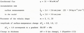
The recent accumulation rate, as determined by β-activity, is 22-24 kg m−2 year−1, which corresponds to 2.4–2.6 cm year−1 of ice (Young and others, 1982). In this study, we assume a constant accumulation rate between Ridge Β (ice divide) and Vostok.
Surface and bedrock topography
For the Vostok area, surface elevation (E) and thickness (H) are taken from the Antarctic map folio (Drewry, 1983). For Vostok Station, we use the more precise data from Kapitsa (1964): E = 3490 m and Η = 3700 m. In this work, H, E, and all depths are expressed in metres of ice. The firn layer is therefore replaced by an equivalent layer of ice with a density ρi = 0.916. The difference between depth in metres ice
(a) Temperature profile measured in the Vostok bore hole. (b) Difference between measured values and a smoothed curve (spline approximation).

equivalent and true depth from the surface is 30 m.
Model Description
Governing equations
The flow lines are assumed to be along the steepest surface slope that is perpendicular to the elevation contours as given in Drewry (1983). In the Vostok area, such flow lines are almost parallel, indicating that the transverse velocity is very small and hence the transverse advection term can be neglected. Consequently, the temperature distribution at Vostok can be reasonably computed using a two-dimensional model with the x-axis defined along the flow line.
The heat equation is solved both for the ice and for a 5 km thick layer of underlying bedrock in order to simulate the geothermal heat-flux changes induced by climatic variations (Ritz, 1987). The heat equation for ice is given by:

Equation (2) is the corresponding equation for the bedrock:
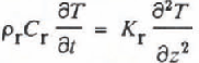
Here, x is the distance from the ice divide, z is the vertical coordinate, positive downward from sea-level, u and w are the horizontal and vertical components of the velocity, Q is the strain heating in the ice, ρ is the density, C is the specific heat, and Κ is the thermal conductivity (subscript i for ice and r for rock). The values of these parameters are given in Table I.
Numerical methods
In order to avoid computational problems at the boundaries, the vertical coordinate z is transformed to a relative coordinate

Boundary conditions
The temperature (Ts) is defined at the ice surface according to the Vostok record (see climatic history), and a constant geothermal flux (φ) is defined at the base of the rock layer (5 km below the ice-rock interface). East Antarctica is generally assumed to be a Precambrian shield with typical heat-flux values of 40 ± 10 mW/m2 (Lee, 1970). However, near Vostok, the bedrock shows subglacial highlands, indicating that this area may have had a more complex geological history (Drewry, 1975) with a higher geothermal flux.
Model simulations were therefore performed with φ values between 35 and 90 mW/m2.
At the ice-rock interface, three types of boundary condition are used depending on (Tb), the basal temperature. When Tb is below the melting temperature, the heat flux across the ice-rock interface is continuous and the boundary condition is given by Equation (3).

When ice at the interface is at its melting point, the melting temperature is prescribed and the melting rate


where L is the latent heat of fusion. A third type of base is the “temperate basal layer”, in which the ice is at its melting point in a basal layer as well as at the ice—rock interface (Lliboutry, 1987). In our model, the occurrence of such a base is tested but it has never been found in the Vostok area.
Velocity field
Following Lliboutry (1981), the horizontal velocity (u) is written

where Ū is the balance velocity and m is a parameter describing the shape of the velocity profile with depth. Using the Lliboutry model, m is about 11 in the Vostok area. In order to study the sensitivity of the model to the velocity shape, the computation is also performed using m = 5 and m = 20.
The balance velocity is obtained by solving numerically the mass-continuity equation at each time step:

where Ṁ is the melting rate, computed using Equation (4). ḃ (the accumulation rate) and H (the ice thickness) are both functions of time (see climatic history).
The vertical velocity (w) is computed using the ice-incompressibility equation:


to the bottom

Following Lliboutry (1987), we assume that sliding is significant only in the case of a temperate basal layer. As this condition does not appear in the Vostok area, u(x, 1) is taken to be equal to 0. The velocity profiles with depth at Vostok are given in Figure 2. Note that vertical velocity is much less sensitive to the value of the exponent m than is horizontal velocity. Note that in Equations (6), (7), and (8) ḃ and Ṁ are expressed in m (of ice)/year.
Physical parameters for ice and rock; Τ is temperature in °c

Velocity profile with depth with different values of m. (a) Horizontal velocity, and (b) vertical velocity.

Strain heating
The heating released by deformation within the glacier is:

where g is the acceleration due to gravity, and

Strain heating is concentrated at the base of the ice sheet. For instance, from Equations (5) and (9), and with m = 11, 20% of the total strain heating is produced in a basal layer representing 1/60 of the ice thickness. This layer corresponds to 1/2 vertical step above the ice-rock interface. Using the finite-difference method, heat production is not taken into account at the interface node and therefore in this layer. This is because the boundary condition applies instead of the heat equation where Q is introduced. To avoid this systematic error, a heat flux φd is added to


where h is the vertical step (h = H/30).
Climatic history
The continuous deuterium record from the Vostok ice core has been used to reconstruct the palaeotemperature record for the Vostok area over the last 160 000 years (Jouzel and others, 1987). From the 6D record, past surface temperature has been estimated and reported relative to the present-value gradient of 6‰ per °C. The authors estimated that the error in the temperature change can be up to 20%. In order to determine the sensitivity of our results to this parameter, the model was run with three values of the temperature-variation amplitude: ΔTS = 0.8, 1, or 1.2 (ΔTS = 1 corresponding to a gradient of 6‰). In this study, we use the smoothed palaeotemperature curve given by Jouzel and others (1987), corrected for temperature variations due to different ice origins. As the palaeotemperature record gives the past surface temperature even in those cases of thickness change, the only correction needed is that which arises from the difference in elevation between Vostok and the location of ice origin. This later correction was made using the velocity field described above.
The smoothed palaeotemperature curve is suited to this model because high-frequency temperature oscillations are damped by heat diffusion in ice. However, very recent surface-temperature variations may affect the upper part of the down-core temperature profile. In order to assess the influence of such variations, some computations are performed for the last 5000 years with a less smoothed surface-temperature record.
Changes in the accumulation rate can be estimated from the Vostok palaeotemperature record. If one assumes (Robin, 1977) that the accumulation rate is governed by the amount of water vapour contained in the air, the accumulation rate is then proportional to ∂P/∂T, where Ρ is the water-vapour pressure at the condensation temperature (Tc). The palaeo-accumulation rate (ḃt) can therefore be estimated given the present-day accumulation rate (ḃ0) and the palaeotemperature using Equation (11).

The condensation temperature (Tc) is taken to be the temperature at the top of the inversion layer. At Vostok, the mean value of inversion is −16.6°C (Kovrova, 1964). According to Jouzel and others (1987), the variations in condensation temperature can be derived from changes in the surface temperature using the empirical relation ∂T c/∂T s=0.67. The accumulation-rate changes obtained in this way are in good agreement with those estimated from the 10Be profile (Raisbeck and others, 1987). From Equation (11), accumulation rate as a function of time is described entirely using the present value (ḃ0) and the palaeotemperature.
The last parameter related to climatic change is the ice thickness. A first-order approximation of the maximum change in thickness is obtained by assuming that the horizontal velocity does not vary during a climatic cycle. This neglects the influence of temperature on ice flow and changes in basal stress due to thickness variations.

Because the accumulation rates between Vostok and Ridge Β are supposed to be identical, ∂H/∂x must be almost constant over time and the mass-continuity Equation (6) then gives:

where ḃm is the average value of ḃ over a climatic cycle. This relation was used to test the sensitivity of the computed temperature profile to change in ice thickness by running the model for two cases: no variation (∂H/∂t) and maximum variation (Equation (12)).
Variations in surface temperature, accumulation rate, and ice thickness over 160 000 years (duration of the Vostok record) are presented in Figure 3. In order to decrease the influence of the initial temperature field, the model is run over several climatic cycles.
Results
Method
The model described above is used with a number of different sets of parameters. Table II lists the different parameters and their range of variation.
Comparison between the computed and observed temperature profile is first done by calculating the standard deviation (σ) and the difference of the means (ϒ)

where T0 is the smoothed observed temperature and Tm is the computed temperature, both taken at the depths z(i) corresponding to the nodes of the model. As temperature profile is measured between 0 and 2010 m (ice equivalent), only the first 17 nodes of the computed temperature are used (N = 17). The “best fits” are given by a minimum σ, while ϒ is useful in determining whether the computed temperature is globally colder (ϒ < 0) or warmer (ϒ > 0) than the observed one.
Standard tests
The first computations are performed with ΔTs = 1, ΔH = 1, and m = 11 which are the more plausible values of these parameters. The study then concerns accumulation rate and geothermal flux. Figure 4 shows σ and γ versus φ for several values of ḃ0.
When φ is less than 50 mW/m2, the computed profile is much lower than the observed one. With such values, one cannot simulate the measured temperature profile with any accumulation rate. This provides a minimum value for geothermal heat flux of 50 mW/m2. We also note that, in
Standard deviation and mean of (Tcomputed - Tobserved) versus geothermal flux for different values of present accumulation rate.

those cases where φ < 50 mW/m2, basal temperature is below the melting point. With larger values of geothermal flux, basal ice reaches the melting point and agreement between calculated and measured profiles can be very good with σ values equal to 0.05°C. The minimum geothermal flux necessary to obtain good agreement is dependent on the accumulation rate. Minimum φ values range from 54 mW/m2 for ḃ0 = 2.3 cm/year to 67 mW/m2 for ḃ0 = 2.6 cm/year. This behaviour is expected because higher accumulation rates require a larger geothermal flux to compensate for the cooling due to the advective process.
When φ is larger than 65 mW/m2, melting is important with consequent increase in the vertical velocity as well as advection at the base (Equations (4) and (8)). This effect is clearly seen in Figure 4 where the highest φ values correspond to relatively cold computed profiles. The maximum in each γ curve occurs not as soon as melting is initiated but only when it occurs during almost the whole climatic cycle, because there is competition between this process (which is not very efficient) and the warming effect of heat flux which prevails when the base is cold.
Parameters of the model and their range of variation
The maximum in γ corresponds to the warmest calculated profile that it is possible to obtain with a given accumulation rate. For low accumulation rates, this maximum is positive, yielding two different best fits (γ = 0), the second one being for a high melting rate. If accumulation rate is higher than 2.55 cm/year, the computed profile is colder than the observed one for any heat flux. In this case, the basal melting point is reached but an advective process removes heat in the upper part of the ice sheet. This result is interesting as it provides an upper limit for the accumulation rate. With the “standard” set of parameters, this limit is 2.6 cm/year which agrees well with surface measurements (Young and others, 1982).
In summary, one can estimate the minimum value of γ and a maximum accumulation rate from a comparison between the computed and the observed temperature profiles. On the other hand, it is not realistic to derive a maximum value of the geothermal flux from these model results. Indeed, Equation (8) which gives the basal velocity as a function of melting assumes implicitly that all the water produced by melting penetrates into the substrate. This is not always the case and must depend on the type of substrate underlying the glacier. Robin and others (1977) found the existence of a subglacial lake at Vostok, indicating that some water does not in fact penetrate the underlying substrate. In this case, Equation (8) gives only the maximum value of basal vertical velocity and it is not possible to link geothermal flux and temperature.
The following studies will determine whether these conclusions are sensitive to the other parameters of the model.
Sensitivity to the amplitude of surface-temperature change
The model is run with ΔTS = 0.8 and ΔTS = 1.2, γ and ḃ0 varying as in the previous section. When the amplitude of the surface-temperature change (ΔTS) is smaller than the standard (ΔTS), the computed profile is warmer because the reference is taken at the present time and such an assumption implies the surface temperature was warmer during the ice age. The reverse reasoning can be made for ΔT = 1.2.
The results of these model runs are very similar to those with ΔT = 1. It is possible to simulate the temperature profile only if the base is at the melting point. The main effect of changing ΔTS is to move the limits on ḃ0 and φ. Figure 5 shows, for different geothermal fluxes, the values of ḃ0 giving a good simulation of observation versus ΔTS. For ΔTS = 1.2, the maximum accumulation rate is 2.25 cm/year, which is lower than the field measurements, and a geothermal flux of about 70 mW/m2 is needed. For ΔTS = 0.8, the maximum ḃ0 is 2.9 cm/year.
Values of present accumulation rate giving the best simulation of observation versus ΔTS, the amplitude of surface-temperature change (for geothermal flux = 53, 55, 60, and 65 mW/m2). In grey, the accumulation rate is too high and no fit can be achieved.

Values of present accumulation rate giving the best simulation of observation versus m, the parameter describing the velocity shape (for geothermal flux = 53, 55, 60, and 65 mW/m2). In grey, the accumulation rate is too high and no fit can be achieved.

Influence of velocity shape
The sensitivity to the velocity-shape parameter (m) is presented in Figure 6. For these model runs, changing the parameter also moves the limits. For example, a low value of m corresponds to a lower vertical velocity and hence less advection which must be balanced by higher accumulation rates to obtain the same result. This effect is small but, as we have already noticed, vertical velocity is not very sensitive to changes in m.
Our conclusion is that, given the uncertainty in the value of accumulation rate, it is not possible to obtain information about the velocity shape at Vostok. The case may be different at an ice divide, where the range of plausible shape is larger (Bolzan, 1985), or near the coast where horizontal advection is important and is affected more by the value of m than is vertical advection.
Effect of thickness change
Calculations are also performed with ΔH = 0 (no thickness change). This affects the temperature in two different ways. First, with ΔH = 0, the surface vertical velocity follows accumulation rate (Equation (7)) and changes more than in the standard case. For instance, it is greater during the Holocene than during the glacial periods. From that, we can expect a colder temperature in the upper part of the ice sheet. Secondly, ice is warmer when thickness is greater because of the insulating effect and, during the Holocene, H is larger if no change is assumed (see Fig. 3). The two influences balance each other and, finally, temperature profiles differ by less than 0.2°C between the two cases (ΔH = 1 and ΔH = 0).
Graphical comparison
The differences (T0 - Tm) between the observed and the calculated temperatures is plotted against depth. Figures 7 and 8 present the influence of the different parameters: Figure 7 shows the effect of changing the geothermal flux for a given accumulation rate (ḃ0 = 2.5 cm/year); Figure 8 shows the effect of changing the accumulation rate (with φ = 60 mW/m2). All these computed curves reach the melting point of ice at the base. One can see that the shape of the curve remains the same regardless of the parameter chosen. In Figure 9, we select a few best fits with different values of ΔTS and ḣ0. All the curves are very similar with the difference between observed and computed temperature not exceeding ±0.1°C. However, they have some oscillations. In order to check whether these oscillations could be due to recent surface-temperature variations not taken into account by the smoothed palaeotemperature record, the model was run with a more detailed record over the last 5000 years using a 10 year time step. This palaeotemperature record was obtained by using a less smoothed spline approximation of isotope data. The result of this experiment is shown in Figure 10. The
Influence of geothermal flux. Difference between observed and computed temperature versus depth, for φ = 55 (a), 60 (b), 65 (c), 70 (d), and 75 (e) mW/m2. For all the curves, ḃ0 = 2.5 cm/year and ΔTS = 1.

Influence of accumulation rate. b0 = 2.3 (a), 2.4 (b), 2.5 (c), and 2.6 (d) cm/year. For all the curves φ = 60 mW/m2 and ΔT5 = 1.

Best fits between observed and computed temperature profiles, (a) ḃ0 = 2.5 cm/year, ΔTS = 1, φ = 60 mW/m2; (b) ḃ0 = 2.3 cm/year, ΔTS = 1, φ = 55 mW/m2; (c) ḃ0 = 2.55 cm/year, ΔTS = 0.8, φ = 55 mW/m2; (d) ḃ = 2 cm/year, ΔTS = 1.2, φ = 60 mW/m2.

Influence of the palaeotemperature curve used in the model; (a) with a smoothed curve (standard), (b) with a detailed record.

first 700 m of the computed temperature profile seem to be affected by only 0.03°C. One explanation of this (small) discrepancy between observed and computed temperature profiles could be that the isotope record does not give a sufficiently precise surface-temperature record for the recent years. The difficulty of extracting the climatic signal in the first 100 m has been documented by Benoist and others (1982).
Conclusion
Our model gives a temperature distribution with depth that agrees within 0.1°C of the measured temperature in the bore hole. The computed profile shows that melting occurs at the ice—rock interface which also agrees with the presence of a subglacial lake near Vostok Station. It is possible to obtain a good fit with several combinations of the model parameters, but certain values of geothermal flux and of accumulation rate can be excluded.
The minimum value of the geothermal flux is 50 mW/m2 and is slightly greater than that usually assumed for the Precambrian shield (40 mW/m2). This difference seems small but it considerably affects the temperature distribution and consequently the velocity because of the ice-deformation dependence on temperature. For instance, with a flux of 40 mW/m2 the basal temperature is about −15°C, leading to a five times smaller horizontal velocity than one obtains by using the observed temperature profile. This result confirms the Budd and Young (1983) analysis of the upper part of the measured temperature profile.
A maximum value for accumulation rate is also deduced. This value is dependent on the transfer function used to determine the surface temperature at Vostok from the deuterium record. With the standard transfer function (∂D/∂T=6%₀), the model-predicted maximum accumulation rate corresponds exactly to the upper limit of the accumulation-rate measurements.
It is interesting to note that none of the standard parameters can be excluded. This conclusion is especially important for the chronology of the Vostok record which is very sensitive to the accumulation rate. The upper limit for the accumulation rate found in this work confirms the dating given by Lorius and others (1985).
Acknowledgements
This study was initiated by the Programme National d’Étude de la Dynamique du Climat (CNRS). I thank Professor L. Lliboutry, Professor W. Budd, R. Jenssen, D. Dahl-Jenssen, M. Vallon, and T. Sowers for stimulating discusssions.



