

1. Introduction
The Belt and Road Initiative (BRI) is a strategy proposed by China for infrastructure development and investment in 65 countries in Europe, Asia, and Africa (Chin and He, Reference Chin and He2016), where 30% of world GDP is produced by 64% of the world's population (Huang, Reference Huang2016). Unbalanced economic and population growth implies that agriculture plays an important role in maintaining the national economies of these BR countries, including the livelihoods of farmers. In China, agricultural output has grown rapidly since the 1980s. However, agricultural production still faces the challenge of high costs and low benefits for various reasons such as limited resources and diminishing marginal efficiency of fertilizer use. In particular, there is potential for agriculture in these countries to benefit from moving up the global value chains (GVCs) to receive a higher share of value added (VA) (Zhang and Tang, Reference Zhang and Tang2018). Hence, the present study will examine whether and to what extent the share of the GVCs of the agricultural products of China and these BR countries could increase if trade barriers among them were reduced in the spirit of the BRI.
Generally, developed countries stay at higher positions in GVCs and obtain higher VA (Tang and Zhang, Reference Tang and Zhang2009). In contrast, developing countries including China and most BR countries stay at lower positions in GVCs and obtain lower VA. The BRI, unveiled in 2013, may have improved the positions of China and the BR countries in GVCs. The trade in agricultural products among these countries has increased considerably over time. In 1998, China exported agricultural products valued at only USD 2.606 billion to the BR countries. By 2017, the exports had increased to USD 22.683 billion, nearly 10 times the export volume of 20 years earlier. To explore the potential development opportunities for trade between China and the BR countries, we assume that the BRI impacts can be mimicked by reduction in trade barriers, including both non-tariff barriers (NTB) and tariff barriers (TB), where the reduced NTB captures a potential reduction in trade costs induced by the BRI, and the reduced NB captures the features of an agreement similar to a Free Trade Agreement (FTA), which the BRI countries are expected to enter in the long term (State Council, 2015). We estimate the potential reduction in trade barriers between the BR countries based on historical data and previous studies. Furthermore, we design and simulate scenarios in a global computable general equilibrium (CGE) model to identify the impact of the reduction in trade barriers on the value chains of agricultural products.
Note that the BRI is not equivalent to a reduction in tariffs and non-tariff measures. The BRI seeks to connect the BR countries via land and maritime networks to improve regional integration, increase trade, and stimulate economic growth. The initiative prioritizes five major aspects: policy coordination; infrastructure connectivity; unimpeded trade; financial integration; and connecting people. While not all of the five aspects directly address trade barriers, they can remove certain non-tariff trade barriers by, for example, significantly reducing trade costs. As shown by de Soyres et al. (Reference De Soyres, Mulabdic, Murray, Rocha and Ruta2019), the trade costs for the BR countries will be reduced by 1.5–2.8% due to the transport infrastructure investments of the BRI. Rather than simulating the whole effect of the BRI, this article attempts to study only the impact of reduced trade barriers on the global value chain of agricultural products in the BR countries.
Compared to previous studies, this study considers reductions of both tariff and non-tariff barriers at different levels, besides the extreme case of no trade barriers. The reduction in trade barriers is also based on historical data and relevant studies. Notice that the BRI impact estimated in this study may be underestimated since the reduction of trade barriers captures only the trade costs potentially reduced by the BRI. On the other hand, the BRI impact may be overestimated to some extent because we do not consider the costs of investments induced by the BRI.
2. Literature Review
Previous studies on GVCs have focused on macro-level issues such as the reconstruction of value chains (Strange and Zucchella, Reference Strange and Zucchella2017) and GVC integration (Beverelli, et al., 2019). At the industrial level, most studies have focused on industrial manufacturing (Strange and Zucchella, Reference Strange and Zucchella2017), the financial services industry (Zhang and Tang, Reference Zhang and Tang2018; Amendolagine et al., Reference Amendolagine, Presbitero, Rabellotti and Marco2019) and high-tech industries (Rehnberg and Ponte, Reference Rehnberg and Ponte2018). Some studies have focused on agricultural products, mainly the processing of agricultural products (Gao and Xu, Reference Gao and Xu2016; Hu and Chen, Reference Hu and Chen2018); these studies have enhanced our understanding of the agricultural value chain. However, to our knowledge, no study has quantitatively considered the potential impact of the BRI on agricultural value chains in China and the BR countries, although some studies have estimated the potential impact of the BRI on agricultural trade (e.g. Ma et al., Reference Ma, Balezentis, Zhao and Fang2017). This study extends four streams of the previous studies.
The first stream is about the valuation of regional positions in agricultural value chains. Antràs and Chor (Reference Antràs and Chor2018) summarized several measures to capture the up- or downstreamness of countries and industries in GVCs. Meng et al. (Reference Meng, Peters, Wang and Li2018) estimated the potential environmental costs in GVCs from the perspectives of production, consumption, and trade. Wang et al. (Reference Wang, Wei, Yu and Zhu2017) found that the co-movement with global GDP growth of complex GVC activities was stronger than the co-movement of other types of production activities. Johnson (Reference Johnson and Measuring Global Value Chains2018) distinguished macro- and microapproaches for measuring GVCs and highlighted the contact points between them. He concluded that further convergence between these two approaches could better portray GVCs empirically. Bernhardt and Pollak (Reference Bernhardt and Pollak2016) found that upgrading of industries through participation in GVCs might not be realized for everyone.
The second stream is about the role of regional factors in value chains. Dollar et al. (Reference Dollar, Ge and Yu2016) showed that institutional variations, including the rule of law and political stability, could determine nations’ involvement in GVCs. Evidence from China suggest that local institutions also affect firms’ participation in GVCs (Dollar et al., Reference Dollar, Ge and Yu2016). Amendolagine et al. (Reference Amendolagine, Presbitero, Rabellotti and Marco2019) investigated how foreign investors interact with local countries in GVCs. Beverelli et al. (Reference Beverelli, Stolzenburg, Koopman and Neumueller2019) studied the role of Domestic Value Chains (DVCs) for GVC integration. Rehnberg and Ponte (Reference Rehnberg and Ponte2018) showed that widespread adoption of 3D printing could affect the restructuring, upgrading, and distributing of VA along manufacturing GVCs. Strange and Zucchella (Reference Strange and Zucchella2017) assessed how the widespread adoption of new digital technologies might influence the location and organization of activities within GVCs.
The third stream concerns the value chain of agricultural products in the context of the BRI. Huang et al. (Reference Huang, Liu and Feng2018) showed considerable fluctuations of intensive and extensive margins in China's agricultural product exports to the BR countries, where the extensive margin played a major role in promoting exports. Zhan (Reference Zhan2018) noted the increasing network density of agricultural product exports, competition, and complementarity in the BR countries, as well as the relatively weak position of China in the agricultural value chain in the BR countries, compared to the positions of India, Russia, and Poland. Yu et al. (Reference Yu, Liang and Gao2016) also showed that China's agricultural trade is generally at a disadvantage compared with South Asia. Li et al. (Reference Li, Sun and Tian2018) concluded that comprehensive examination would be necessary to study the regional position of the BR countries in GVCs due to characteristics including high passiveness, strong dependence, significant gradient, and resource orientation. On the other hand, some researchers have questioned the role of the BRI in the promotion of positions in the value chain in general. For example, Ma and He (Reference Ma and He2018) showed that, from the perspective of the BR countries, integration into GVCs does not promote the upgrading of industrial structure.
The last stream is about the impact of trade barriers on GVCs based on CGE models. Most of the studies in this stream focus on FTAs or international organizations. For example, Cai et al. (Reference Cai, Zhang and Meng2015) used a GVC-based CGE model to assess the impact of the TTIP (Transatlantic Trade and Investment Partnership) between the US and the EU. Their results indicate that the TTIP will have a positive impact on global trade and the economy due to the reduction in tariff barriers and non-tariff barriers. Ferraz and Ribeiro (Reference Ferraz and Ribeiro2018) used member states of the Mercosur and China as examples to explore the impact of changes in non-tariff barriers on GVCs using a CGE model. Their results showed that the formalization of preferential trade agreements with natural trade partners may pave the way for Brazilian industry to integrate into GVCs. Fusacchia et al. (Reference Fusacchia, Antimiani and Salvatici2021) used a CGE model focusing on Italy to explore the impact of tariffs on exporting companies that rely on imported intermediate products in the context of GVC.
To the best of our knowledge, no study has addressed the impact of trade barriers reduction on GVCs in the regions along the Belt and Road based on a CGE model. Our study fills in the knowledge gap on this issue. In this article, we adopt the plausible valuation indicators developed by studies in the first stream to address how the value chain of agricultural products in the context of the BRI (the third stream) might be influenced by reduction in trade barriers, which is one of the factors affecting regional positions in the value chain that is discussed in the second stream. Our study is also a new CGE modeling example addressing the impact of trade barriers on GVC, which is relevant to the fourth stream in the literature.
3. Data and Methods
3.1 Measurement of the GVCs of Agricultural Products
A GVC position index refers to the relative position (upstream or downstream) of a country (or industry) in a GVC when participating in global economic activities. Previous studies have adopted a variety of methods to estimate a country's position in GVCs. These methods include: (1) the traditional export trade data statistics method (Qiu et al., Reference Qiu, Ye and Sun2012); (2) the vertical specialization index method (Hummels et al., Reference Hummels, Ishii and Yi2001; Yu and Deng, Reference Yu and Deng2014); (3) the value-added trade measurement method (Koopman et al., Reference Koopman, Powers, Wang and Wei2010, Koopman et al., Reference Koopman, Wang and Wei2014); (4) the net trade index (NET) measure method (Tang, Reference Tang2015); and (5) the import and export unit price comparison method (Mulder et al., Reference Mulder, Paillacar and Zignago2009; Lin and He, Reference Lin and He2015). Following Koopman et al. (Reference Koopman, Powers, Wang and Wei2010) and Wang (Reference Wang2014), the global value chain of agricultural products is interpreted as the global chain of added value generated from international trade in the agricultural products. Hence, the added value obtained by a country from international trade is used to calculate the GVC position of the country at a sectoral level such as agriculture. Assume the world includes G countries and each country produces tradable goods in N sectors. In each sector, goods can be used as intermediate inputs in production activities and to meet final demand from both domestic and foreign economic agents:
 $$x_{is} = \mathop \sum \limits_{\,j = 1}^N a_{ijss}x_{\,js} + \mathop \sum \limits_{r\ne s}^G \mathop \sum \limits_{\,j = 1}^N a_{ijsr}x_{\,jr} + y_{iss} + \mathop \sum \limits_{r\ne s}^G y_{isr}, \;\;\;i\in ( {1, \;N} ) , \;s\in ( {1, \;G} ) $$
where xis is the total output of sector i in country s; aijsr is the direct input–output (IO) coefficient describing units of the product of sector i produced in country s and consumed in the production of one unit gross output of sector j in country r; and yisr is the final demand in country r for goods of sector i produced in country s. Eq. (1) can be written in matrix form,
 $$\left[{\matrix{ {X_1} \cr {\matrix{ {X_2} \cr {X_3} \cr {X_4} \cr } } \cr } } \right] = \left[{\matrix{ {\matrix{ {I-A_{11}} & {-A_{12}} \cr } } & \cdots & {-A_{1G}} \cr {\matrix{ {-A_{21}} & {I-A_{22}} \cr } } & \cdots & {-A_{2G}} \cr {\matrix{ {\matrix{ \cdots \cr {-A_{G1}} \cr } } & {\matrix{ \cdots \cr {-A_{G2}} \cr } } \cr } } & {\matrix{ \cdots \cr \cdots \cr } } & {\matrix{ \cdots \cr {I-A_{GG}} \cr } } \cr } } \right]^{{-}1}\left[{\matrix{ {\mathop \sum \limits_r^G Y_{1r}} \cr {\mathop \sum \limits_r^G Y_{2r}} \cr {\matrix{ \cdots \cr {\mathop \sum \limits_r^G Y_{Gr}} \cr } } \cr } } \right]$$
where Xs is the sectoral gross output vector of country s; Asr is the IO coefficient matrix indicating intermediate inputs from country s to country r Footnote 1; and ysr is the vector of final demand in country r produced in country s. The Leontief inverse matrix (or total requirement matrix) can be expressed by
 $$B = \left[{\matrix{ {\matrix{ {B_{11}} & {B_{12}} \cr } } & \cdots & {B_{1G}} \cr {\matrix{ {B_{21}} & {B_{22}} \cr } } & \cdots & {B_{2G}} \cr {\matrix{ {\matrix{ \cdots \cr {B_{G1}} \cr } } & {\matrix{ \cdots \cr {B_{G2}} \cr } } \cr } } & {\matrix{ \cdots \cr \cdots \cr } } & {\matrix{ \cdots \cr {B_{GG}} \cr } } \cr } } \right] = \left[{\matrix{ {\matrix{ {I-A_{11}} & {-A_{12}} \cr } } & \cdots & {-A_{1G}} \cr {\matrix{ {-A_{21}} & {I-A_{22}} \cr } } & \cdots & {-A_{2G}} \cr {\matrix{ {\matrix{ \cdots \cr {-A_{G1}} \cr } } & {\matrix{ \cdots \cr {-A_{G2}} \cr } } \cr } } & {\matrix{ \cdots \cr \cdots \cr } } & {\matrix{ \cdots \cr {I-A_{GG}} \cr } } \cr } } \right]^{{-}1}$$
where Bsr denotes the N × N block Leontief inverse matrix. Furthermore, we define a direct value-added coefficient matrix by
 $$\hat{V} = \left[{\matrix{ {\matrix{ {\widehat{{V_1}}} & 0 \cr 0 & {\widehat{{V_2}}} \cr } } & {\matrix{ \cdots & 0 \cr \cdots & 0 \cr } } \cr {\matrix{ \cdots & \cdots \cr 0 & 0 \cr } } & {\matrix{ \cdots & \cdots \cr \cdots & {\widehat{{V_G}}} \cr } } \cr } } \right]_{( {GN \times GN} ) }$$
where each element ( $\hat{V}_s$) shows the share of direct domestic value added in total output in country s. Similarly, the global export matrix can be defined by
 $$\hat{E} = \left[{\matrix{ {\matrix{ {\widehat{{E_1}}} & 0 \cr 0 & {\widehat{{E_2}}} \cr } } & {\matrix{ \cdots & 0 \cr \cdots & 0 \cr } } \cr {\matrix{ \cdots & \cdots \cr 0 & 0 \cr } } & {\matrix{ \cdots & \cdots \cr \cdots & {\widehat{{E_G}}} \cr } } \cr } } \right]_{( {GN \times GN} ) }$$
where each element ( $\hat{E}_s$) shows sectoral gross exports in country s. Hence, the value-added of country-sectoral exports can be decomposed as follows:
 $$\hat{V}B\hat{E} = \left[{\matrix{ {\matrix{ {{\hat{V}}_1B_{11}{\hat{E}}_1} & {{\hat{V}}_1B_{12}{\hat{E}}_2} \cr {{\hat{V}}_2B_{21}{\hat{E}}_1} & {{\hat{V}}_2B_{22}{\hat{E}}_2} \cr } } & {\matrix{ \cdots & {{\hat{V}}_1B_{1G}{\hat{E}}_G} \cr \cdots & {{\hat{V}}_2B_{2G}{\hat{E}}_G} \cr } } \cr {\matrix{ \cdots & \cdots \cr {{\hat{V}}_GB_{G1}{\hat{E}}_1} & {{\hat{V}}_GB_{G2}{\hat{E}}_2} \cr } } & {\matrix{ \cdots & \cdots \cr \cdots & {{\hat{V}}_GB_{GG}{\hat{E}}_G} \cr } } \cr } } \right]_{( {GN \times GN} ) }$$
where each element ( $\hat{V}_rB_{rs}\hat{E}_s$) is an N × N block matrix, representing the domestic sectoral value-added in country r embodied in the exports of country s. To sum up the off-diagonal elements along a row, we obtain a country's indirect value-added (IV) embodied in exports of other countries (Eq. (6)). Similarly, to sum up off-diagonal elements along a column, we obtain the foreign value-added (FV) embodied in a country's gross exports (Eq. (7)).
 $$IV_r = \hat{V}_r\mathop \sum \limits_{s\ne r}^G ( {B_{rs}{\hat{E}}_s} ) $$
 $$FV_r = \mathop \sum \limits_{s\ne r} ( {{\hat{V}}_sB_{sr}} ) \hat{E}_r$$
If the IV of a country is high relative to its gross exports, then a relatively large share of the country's exports comes from demand for domestic intermediates induced by the exports of other countries, which indicates the country's upstreamness in the GVC. On the contrary, if the FV of a country is high relative to its gross exports, then a relatively large share of the country's exports goes to the value-added of other countries that export to the country's intermediates, which indicates the country's downstreamness in the GVC. Hence, both indicators should be considered when determining a country's position in the GVC. Following Koopman et al. (Reference Koopman, Powers, Wang and Wei2010), the position in the GVC at a country-sector level is defined by the index
 $$GVC\_position_{ir} = Ln\left({1 + \displaystyle{{IV_{ir}} \over {E_{ir}}}} \right)-Ln\left({1 + \displaystyle{{FV_{ir}} \over {E_{ir}}}} \right)$$
where i represents sector i and r represents country r. The index is valid only if a country participates in international trade, i.e., has positive exports. If the index is large, the country lies upstream in the GVC in the sense that the country obtains more value-added from its exports of intermediates compared to the value-added that another country receives from its exports. If the index is small, the country lies downstream in the GVC. If a country moves from downstream to upstream in the GVC, the country becomes relatively more important as a destination to which other countries export their products, implying a stronger position in the GVC.
In this study, since the Global Trade Analysis Project (GTAP) model described in Section 3.2 does not directly report the value of the GVC position index, we use the relevant results from the model to calculate the GVC based on the above-mentioned method. We compare values of the GVC position index in alternative scenarios to identify changes of a country's position in the agricultural GVC.
3.2 GTAP Model
This study adopts the static version of the GTAP model, a global multi-region, multi-sector CGE model (Hertel, Reference Hertel1997). Key assumptions of this model include: (1) complete market competition; (2) constant return to scale in production; (3) cost minimization for producers; (4) utility maximization for consumers; and (5) market clearing for all products and production factors. The model allocates household consumption, savings, and government consumption to regions according to Cobb–Douglas functions, while distinguishing between domestic and imported products. In particular, the model describes the bilateral import and export between regions. More details about the GTAP model can be found at Hertel et al. (Reference Hertel, McDougall and Walmsley2007).
The GTAP static model in this study is built with a base year of 2011. The base year is only two years ahead of 2013, when the BRI was officially announced, providing a plausible benchmark economy without any BRI impact. To isolate the BRI impacts from any other factors affecting the GVC positions, a comparative static analysis is conducted to examine the BRI impacts by simulating reduction in trade barriers in the 2011 economy in alternative scenarios. We acknowledge that it would be more interesting to provide estimates for the coming years by extending the static model to a dynamic model, to better simulate the impact over time of investments in, for example, infrastructure. However, this study intends to explore the impact of removal of trade barriers rather than the impact of investments. In our case, a dynamic model needs a schedule of stepwise reductions of trade tariffs and non-tariff barriers, which is not available and difficult to assume.
3.3 Data
The GTAP model in this study is based on the GTAP 9 database, which contains the 2011 data for 140 countries (or regions), 57 industries (or products), and eight basic production factors (Aguiar et al., Reference Aguiar, Narayanan and McDougall2016). We aggregate the regions, industries, and production factors to simplify the calculation while still meeting the needs of this study.
In this study, the 65 BR countries are aggregated into seven regions: Central Asia Mongolia and the Commonwealth of Independent States (MCIS), ASEANFootnote 2, West Asia, South Asia, Central and Eastern Europe, and China. All the other regions are treated as one region (rest of the world – ROW).
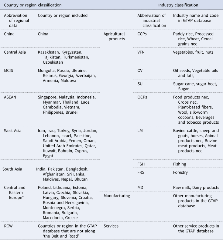
The economy of each country is divided into three major sectors: agriculture, manufacturing, and services. Agriculture is further divided into nine sub-sectors: cereal crops (CCPs); vegetables, fruit, and nuts (VFN); oil crops (OV); sugar (SU); other crops (OCPs); livestock meat (LM); fishery (FSH); forestry (FRS); and milk and dairy products (MD). The detailed classifications are shown in Table 1.
Aggregated regions and sectors based on the GTAP database classification

Note: *In this article, the TB reduction in Central and Eastern Europe is the same as in other regions. This article assumes that these states face lower TB and NTB than other EU member states, although some Central and Eastern Europe countries are part of the EU. These eastern EU member states are affected by BRI much more than the other EU member states in any case. Hence, this article assumes that Central and Eastern Europe has the same TB reduction as other BR regions.
Source: GTAP v9 database and own aggregation.
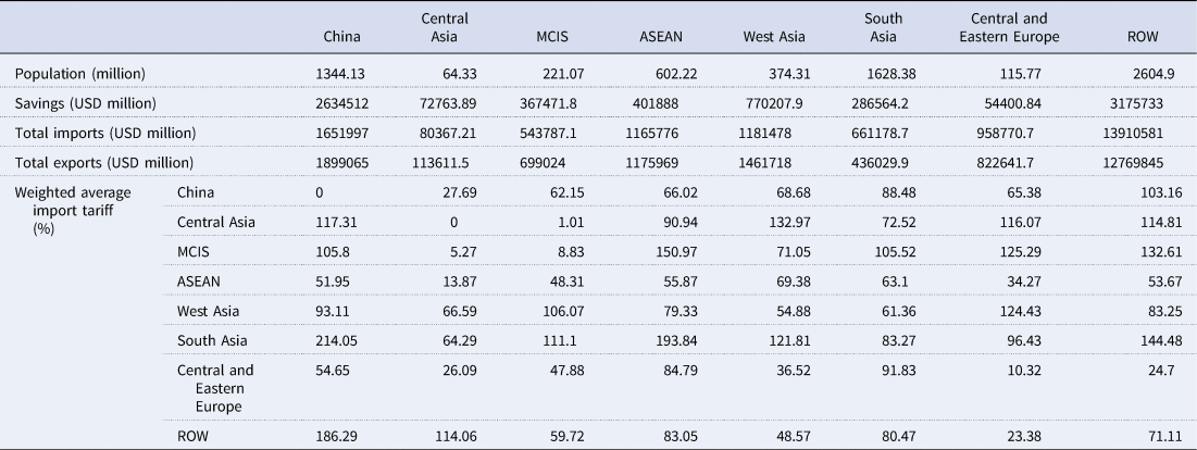
For 2011, the populations, savings, imports and exports, and tariffs of the BR regions are shown in Table 2. The population in South Asia was slightly more than that in China, while the population in ASEAN is slightly less than half of China's population. On the contrary, the amount of savings in China is nine times that in South Asia and 6.6 times that in ASEAN, indicating a dominant role of China in available funding for investments. The regions with the highest total imports among all the BR regions are China, ASEAN, and West Asia, which are also the only regions with total imports exceeding USD 1,000 billion. The regions with the lowest total imports are Central Asia, MCIS, and South Asia, of which Central Asia is the only region that does not exceed USD 100 billion. China's total imports are more than 20 times those of Central Asia, 3 times those of MCIS, and nearly 2.5 times those of South Asia; they account for approximately 8% of the world's total imports. The total imports of all the BR regions accounted for approximately 31% of the world's total imports. In addition, China, ASEAN, and West Asia were the regions with the highest total exports among all the BR regions. The regions with the lowest total exports were also Central Asia, MCIS, and South Asia. China's total exports accounted for about 10% of the world's total exports; these exports exceeded 16 times those of Central Asia. The total exports of all the BR regions accounted for approximately 34% of the world's total exports. The weighted average import tariff varied among the BR regions. The highest tariff level was the import tariff of China against South Asia, where the weighted average import tariff exceeds 200%. The second is ASEAN's import tariffs on South Asia, with a weighted average tariff of 194%. Only a few regions had an import tariff of less than 10%; as an example of these few regions, the import tariff of MCIS on Central Asia was only 1%.
Economic situation of the regions along the route in 2011

Source: GTAP v9 database and own aggregation.
3.4 Trade Barriers in the GTAP Model and Potential Impacts on GVC Positions
We assume that all products being traded among the BR countries enjoy the reduction of trade barriers assumed in the scenarios described in Section 4. In the GTAP model adopted in this study, trade barriers are represented by two parameters of bilateral tariff and non-tariff levels. A change in the tariff level leads to changes in the prices of imported products, which subsequently affect the quantity of the imported products. The NTBs are indicated in the GTAP model by the parameter representing the impact of foreign technology on the country, an increase of which reduces export volume and prices of the corresponding products. The effects of both trade barriers disturb the whole global economic system and finally the economy reaches an equilibrium different from the original one. By comparing the two equilibria, we identify the impact of the reduction in trade barriers for the BR countries on the GVCs of agricultural products.
Notice that the reduction in trade barriers reduces the purchasing prices of imported products and induces more demand for imports to a country. From the perspective of other countries, this means an increase in demand for their exported products, which pushes up the prices of the products being exported from these countries. Hence, the reduction in trade barriers generally reduces the purchasing prices in the importing countries while increasing the producer prices in the exporting countries. If a country has both imports and exports of specific products, then how prices of the product evolve in its domestic market depends on whether the effect of the imports is stronger than that of the exports.
According to the definition in Eq. (8), the position of a country in a GVC depends on exports of all regions and on prices in the international market, which modify both the IV embodied in exports of other countries and the FV embodied in a country's gross exports. A removal of trade barriers among the BR countries can encourage exports among these countries. If barriers are reduced, more intermediate products from one country will be demanded due to the additional exports of the other countries, which leads to more IV embodied in the exports of other countries. On the other hand, additional exports from one country require more intermediate products from other countries, which induces more FV embodied in a country's gross exports. In addition, the changes in prices can affect exports, IV and FV. Hence, it is unclear whether the GVC position of a BR country will move up or not following a removal of trade barriers among the BR countries. However, the GVC positions of the BR countries as a group and of other countries are respectively enhanced and weakened since a removal of trade barriers among the BR countries discourages their trade with the other countries.
4. Scenarios
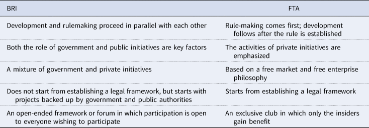
Investments in the BRI countries have been increasing since the BRI was proposed in 2013. Most of the investments have focused on construction of infrastructural facilities in energy and transport (Du, Reference Du2016). These infrastructural facilities could potentially reduce transportation costs and improve the efficiency in logistics to promote trade among the BR countries in the future. The reduction in trade costs can be interpreted as a kind of removal of non-tariff trade barriers. Moreover, the BRI has strengthened communication among the BR countries and increased the degree of integration, creating a better environment to facilitate the negotiations of a free trade agreement among the BR countries, Particularly in the long term, the BRI countries are expected to enter into agreements with the characteristics of an FTA (State Council, 2015) although the characteristics of the BRI and an FTA differ considerably at present, as shown in Table 3 (Chaisse and Matsushita, Reference Chaisse and Matsushita2018).
Characteristics of BRI and FTA

Source: Chaisse and Matsushita (Reference Chaisse and Matsushita2018).
Given the anticipation that the BRI will become an FTA, and its potential to promote bilateral trade between the 65 BR countries, we design several scenarios of reduction in trade barriers to explore the potential implications of the BRI for these countries. It should be noted that TB and NTB are only some of the expected impacts of the Belt and Road Initiative. As mentioned above, previous studies based on the GTAP model typically adopt an extreme scenario where all TB are removed (Chen and Yang, Reference Chen and Yang2015) and the NTB are overlooked. To tackle this issue, we design several scenarios corresponding to different reductions in TB and NTB among the BR countries based on historical trade barrier data. The BRI is expected to improve the trade environment generally among the BR countries without differentiating one sector from another. For example, if a train becomes available between two countries, the reduction in transportation costs for agricultural goods may not differ a lot from that for other goods. In this sense, it is reasonable to assume the same rate of reduction of NTB for all sectors, and higher initial tariffs of a sector should remain relatively higher even after the BRI effect is considered. However, the reduced TB or NTB cannot capture the investment costs; thus, as noted above, this study captures only part of the impact of the investments induced by the BRI.
In this study, to identify the potential impact of reduction in trade barriers, all scenarios are compared to a Reference Scenario, where the actual economy in 2011 described by the GTAP database is regenerated by running the static GTAP model. Hence, our results show what would have occurred if the reduction in trade barriers was implemented in 2011, since effects of future changes in all factors other than the reduction in trade barriers are abstracted from our simulations.
4.1 Best Estimate Scenario
This study mainly focuses on the Best Estimate Scenario, where reductions in both TB and NTB are estimated from historical data and previous studies. In the long term, the BRI countries are expected to enter agreements similar to FTAs (State Council, 2015). Hence, in the Best Estimate Scenario, we assume that all BR countries enjoy the same reduction in trade barriers as those BR countries that currently have FTAs with China. Since the relevant adjustment parameters of TB and NTB are built into the model, this article needs to calculate the specific reduction values of TB and NTB, and then adjust the two parameters in the model. Changes in TB and NTB in the model can have an impact on import and export prices, income, welfare, etc. This affects total volumes of imports and exports until the model reaches a new general equilibrium. Although we consider the joint impacts of the reduced TB and NTB in the ‘Best Estimate’ scenario, the reduced TB and NTB may have different impacts on the economies of different BR countries, as indicated by the simulation results reported in the appendix.
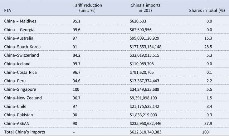
The reduction in TB is estimated by a simplified method derived from Petri et al. (Reference Petri, Plummer and Zhai2012) based on the FTAs that have been signed with China. In our estimate, the tariff reduction is assumed symmetrical in bilateral relationships. Because of data availability, we follow previous studies (Huang and Yu, Reference Huang and Yu2018) to assume that the tariffs of agricultural products in all the BR countries have been reduced at the same rate, which is comprehensively measured from current FTAs between China and 13 FTA countries (or regions) as shown in Table 4,
 $$\Delta tariff = \displaystyle{{\sum tariff_i \times im_i^{2017} } \over {\sum im_i^{2017} }}$$
where Δtariff is the estimated overall tariff reduction in all 65 BR countries (or the 7 BR regions in our model); Δtariffi is the average tariff reduction of China in the FTA with country i, expressed as the share of imports of all FTA duty-free goods in total imports; and  $im_i^{2017} $ represents the imports from country i to China in 2017. Our calculation shows that the average tariff reduction among the BR countries is 92%, meaning 92% imports of all products in the bilateral trade among the BR countries are tax free. In our model, the tariff on all products is assumed to be reduced by 92%.
The FTAs between China and other BR countries (or regions) as of 2018

Note: Tariff reduction is based on data from China FTA Network (http://fta.mofcom.gov.cn/english/index.shtml), accessed on 26 January 2019. Imports in 2017 are from the UN Comtrade database (https://comtrade.un.org/data/).
We also consider reduction in NTB among the BR countries based on the iceberg trade cost approach. Following Petri et al. (Reference Petri, Plummer and Zhai2012), we divide the aspects covered by the FTAs into 24 issue areas and score the reduction in NTB of each area based on the content of the FTAs. The overall reduction of the NTB is then calculated as the weighted sum of the reduction in NTB across the 24 areas. Specifically, the NTB reduction (ΔNTB) is associated with three factors: average score S j, reflecting subjective assessments of the issues in the FTAs; policy weight P j, indicating relative importance of different FTAs for NTS; and coefficient λ,⋅
 $$\Delta NTB = \lambda \mathop \sum \limits_{\,j\in A} P_jS_j$$
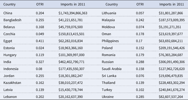
The values of policy weights and average scores are directly from Petri et al. (Reference Petri, Plummer and Zhai2012). The coefficient λ is calculated using the iceberg trade cost based on the Overall Trade Restrictiveness Index (OTRI) (Huang and Yu, Reference Huang and Yu2018). The OTRI data are derived from Looi Kee, et al. (Reference Looi Kee, Nicita and Olarreaga2009) by estimating the ad-valorem equivalents (AVEs) of NTBs for each country at the tariff line level. The OTRI index summarizes the impact of each country's trade policies on its imports, depending on the overall level of protection and the elasticity of import demand and imports. In this paper, the OTRI of a country is weighted by the shares of imports from other countries relative to the gross imports of the country in the base year 2011, i.e.,
 $${\rm \lambda } = \mathop \sum \limits_{i\in N} OTRI_i \times w_i^{import} $$
where OTRI i is the overall trade restrictiveness index of country i, and  $w_i^{import} $ indicates the share of imports from country i relative to the gross imports of all countries in the collection N, where the countries in collection N are the BR countries that have OTRI.
Based on Eq. (10), we adopt the higher scores of S j from Petri et al. (Reference Petri, Plummer and Zhai2012) and the data of imports and OTRIs of countries in collection N (Table 5) to calculate the overall reduction of NTB as 15.36%, which is assumed for all the BR countries in the Best Estimate Scenario.
Countries’ imports and OTRI

Source: The OTRI data are derived from the study by Looi Kee et al. (Reference Looi Kee, Nicita and Olarreaga2009). Imports in 2011 are from the UN Comtrade database (https://comtrade.un.org/data/).
4.2 Two Alternative Scenarios
In the best estimate scenario, we assume a certain level of reduction in trade barriers. However, the assumption might be too optimistic or too pessimistic from the perspective of the potential influence of the BRI on trade barrier reduction. Hence, we also consider two alternative scenarios: one is the pessimistic scenario and the other is the optimistic scenario.
4.21 Pessimistic Scenario
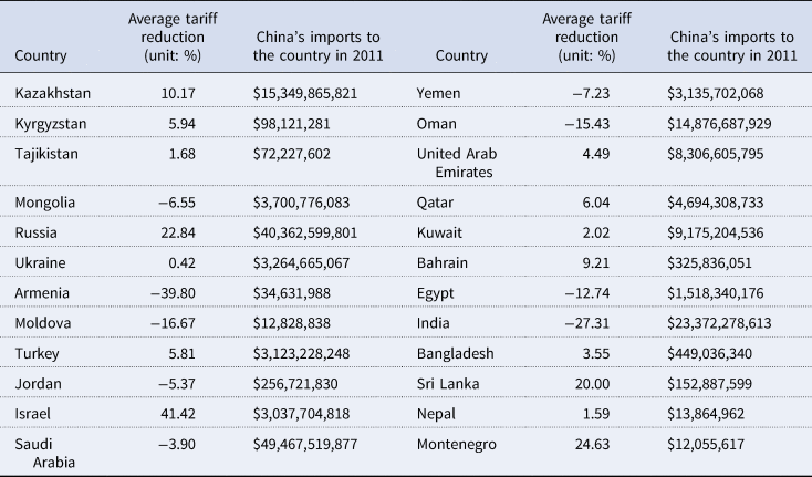
In this scenario, we assume that the effect of BRI on trade tariffs had been fully realized by 2019, meaning there will be no further tariff reductions due to BRI after 2019. We determine the reduction in trade barriers by comparing the trade barriers among the BR countries before and after the BRI was proposed in 2013 (Table 6). We obtain the average import tariff data from the BR countriesFootnote 3 to China in the WTO database and calculate the average tariff in 2011 weighted by the imports of each country in 2011, the same as the base year in our model. The average tariff is taken as the tariff level of China and these BR countries before the BRI. The tariff level after the BRI is then calculated as the average tariff data of the same BR countries still weighted by the imports in 2011 based on the latest tariff data from the WTO database as of February 2019. By comparing the tariff levels before and after the BRI, we obtain an average reduction in trade tariffs of only 1.01%, which is assumed for all the BR countries in the pessimistic scenario.
National tariff reduction and trade data along the BRI route

Source: Tariff level is based on data from WTO Network (http://tao.wto.org/report/TariffAverages.aspx), accessed on 22 February 2019.
Tariff reduction data are from author calculation and the negative signs signal tariff increases. China's imports to the country in 2011 are from the UN Comtrade database (https://comtrade.un.org/data/).
As for the calculation of NTB, the calculation method of formula (10) is still adopted. In order to compare with the Best Estimate Scenario, we adopt the lower scores of S j from Petri et al. (Reference Petri, Plummer and Zhai2012) for the calculation. The reduction of NTB in this scenario appears to be only 10.56%.
4.2.2 Optimistic Scenario
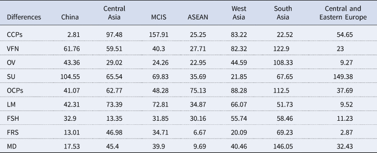
This scenario follows the typical assumptions in previous studies to set the tariffs between the BR countries as zero. Table 7 shows the differences between the weighted average import tariffs of various industries and regions between the optimistic and pessimistic scenarios. For the non-tariff barriers, a reduction by 20% is assumed, which is almost double the reduction level in the pessimistic scenario.
The differences in tariff cuts between the pessimistic and the best estimate scenario. %

4.3 Key Differences between Scenarios
Table 8 summarizes the key assumptions about the reduced TB and NTB in the three scenarios mentioned above. Compared to the ‘best estimate’ scenario, the TB are reduced to a much larger extent than the NTB in the Pessimistic scenario, while the opposite is true in the optimistic scenario.
The assumed reductions of TB and NTB in alternative scenarios

5. Results and Discussion
5.1 Trade Volume and Price
5.1.1 Imports of the BR Countries
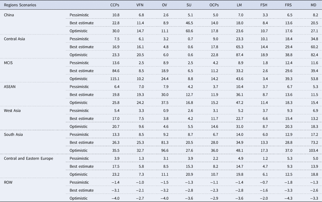
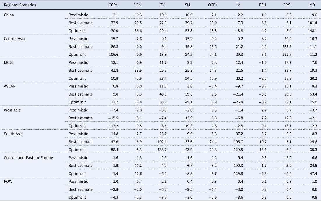
Table 9 shows the deviations of imports from the reference scenario. In the Best Estimate Scenario, the imports of each BR country increase markedly compared to the reference scenario due to relatively lower consumer prices of imported products compared to domestic prices. For example, the imports of LM and MD in Central Asia and MD in South Asia increase by more than 60%, and the imports of CCPs in the MCIS region and OV in South Asia increase by more than 80%. Compared with the pessimistic scenario, where the BRI does not successfully reduce barriers, the increases in imports of most products are considerable. However, the increases in imports in the optimistic scenario are relatively modest compared to the best estimate scenario.
Deviations of imports from reference scenario. %

Source: Own calculations.
5.1.2 Export from the BR Countries
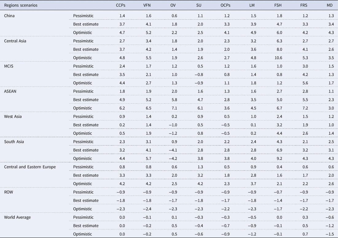
Table 10 shows the deviations of exports from the reference scenario. In the best scenario, exports of most products in most of the BR regions increase considerably due to the reduction in trade barriers. On the contrary, we observe declining exports of most products from the rest of the world. Compared to the two alternative scenarios, we observe similar patterns for imports. However, there are exceptions among certain disadvantaged industries in some countries, such as LM in ASEAN and SU in Central Asia, where the reduction in trade barriers does not increase the export of these products. In these cases, the reduction in trade barriers promotes exports from other countries with relative advantages, plundering the market that originally belonged to the domestic industry in the country, and making it more difficult to export the product. This negative impact increases as the trade barriers are reduced more.
Deviations of exports from Reference Scenario. %

Source: Own calculations.
5.1.3 Export FOB Prices
Table 11 lists the changes in Free on Board (FOB) prices of various agricultural products for exports. The price changes compared to the reference scenario are calculated from corresponding price indices extracted from the modeling results. Notice that the increase in export prices is driven by the stronger demand induced by the reduction in trade barriers, although the consumers in the importing countries face a still lower buying price. In general, the export prices in China increase, while the world average of export prices decline for some products. Most of the agricultural products in the BR countries are exported at higher prices. The comparison with the two alternative scenarios shows that the greater the reduction in trade barriers among the BR countries, the higher the domestic and export prices of agricultural products in China and the BR countries.
Deviations of export FOB prices from the reference scenario. %

Source: Own calculations.
5.2 Value Chain Positions
5.2.1 Regional Level
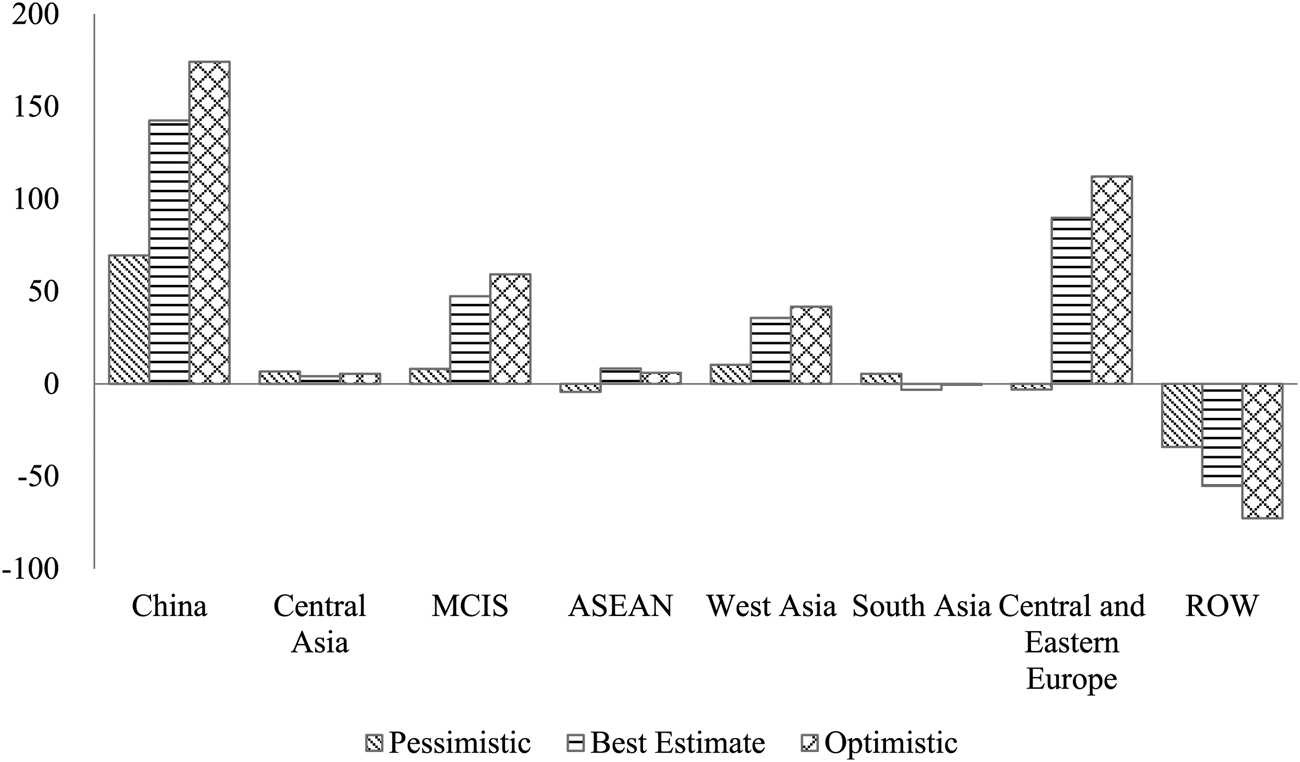
Figure 1 shows the percentage changes in agricultural GVC position at the regional level. Overall, the reduction in trade barriers increases the agricultural GVC position of China and the BR countries. Changes in the GVC position are mainly affected by IV and FV. The reduction of trade barriers causes changes in IV and FV, which shows that GVC is related to both backward and forward linkages. The inter-regional trade becomes easier and the import and export of intermediate goods becomes more frequent with trade barriers reduction. Therefore, the greater the reduction in trade barriers, the better the agricultural GVC position of China and the BR countries. The agricultural GVC position in non-BR countries declines, with the highest decline of 55% in the optimistic scenario. In the best scenario, China's agricultural GVC position increases significantly by 142%. The agricultural GVC position of MCIS, ASEAN, and Central and Eastern Europe increase by over 35%. In other BR regions, most of the agricultural GVC positions increase, with an exception for South Asia in the best estimate scenario. This is because South Asia industries can still trade as before to promote their GVC position in the pessimistic scenario where the trade barriers are reduced. Trade between the BR countries become more frequent with reduced trade barriers (the best estimate). The GVC position of South Asia declines because the comparative advantages of most industries (such as OV, SU, LM) are relatively weak in other BR countries. With the further decline of trade barriers in the optimistic scenario, the comparative advantage of the South Asia industries is improved due to frequent trade exchange; as a result, the GVC position of South Asia is improved. However, the GVC position of South Asia in the optimistic scenario still declines compared with the case without the reduced trade barriers. Hence, the reduction in trade barriers can enhance the agricultural GVC positions of the BR countries in general, although at various rates.
Percentage changes in agricultural GVC position.
Source: Own calculation.

5.2.2 Industry Level
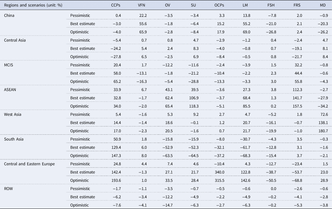
Table 12 lists the changes in the GVC position of various industries in each BR country. For China, the GVC position of many agricultural industries is increased. In the best estimate scenario, the GVC position of the LM industry and VFM industry increase markedly, by more than 55%. The GVC position of the OCPs industry also improves by more than 15%. For other BR countries, the reduction in trade barriers has certain impacts on their agricultural industries’ GVC positions. The GVC positions of comparative advantage industries (CAI) in various BR countries (or regions) are greatly enhanced with the reduction in trade barriers. For example, the GVC positions of South Asia's CCPs industry, Central and Eastern Europe's CCPs industry, ASEAN's SU industry, Central and Eastern Europe's OCPs industry, Central and Eastern Europe's LM industry, and ASEAN's FRS industry increase by 100%. However, the GVC positions of some industries have declined by more than 50%; these include South Asia's OV, SU, and LM industries, and Central and Eastern Europe's FRS industry, due to relatively weak competitiveness.
Changes in GVC position of various industries

Source: Own calculations.
5.3 Sensitivity Analysis
The above results can be determined by the values of key parameters. In this study, the elasticity between domestic and imported products is one of the key parameters since it determines how international trade responds to market price signals. In the GTAP model and other CGE models, the elasticity is called the Armington elasticity of substitution. Table 13 shows the values of the Armington elasticities in the above analysis.
Default Armington substitution elasticities between imported and domestic products by product

Source: GTAP model described by Hertel et al. (Reference Hertel, McDougall and Walmsley2007).
To examine how our results are sensitive to the Armington elasticities, we shift up (or down) the values of all the elasticities in Table 10 by 50%, and run our simulation again for the best estimate scenario to obtain the changes in GVC position, which is compared with the GVC position in the best estimate scenario with the default values of the elasticities in Section 4. Our results show that, with the alternative values of the Armington elasticities, the GVC position of most regions at the regional level changes in the same direction as in the default case shown in Section 4, although the indicated scale of the changes differs, with absolute deviations within 50% of those in the default case.
6. Conclusion
The BRI may potentially provide tremendous opportunities for international trade of agricultural products between China and the BR countries. This study explores the potential impact of the BRI on the GVC positions of the agricultural product industries of the BR countries, by assuming that the BRI leads to reduction in trade barriers. This paper focuses on agricultural trade between China and the BR countries and deepens the understanding of the impact on agricultural GVCs of the reduction in trade barriers implied by FTAs between China and the BR countries.
Based on previous studies and historical data, this paper has estimated the possible reduction of trade barriers, including both tariff and non-tariff barriers, between China and the BR countries in a best estimate scenario and two alternative scenarios. In the best scenario, we estimate the reduction of tariffs on the BR countries by 92% based on the FTAs currently signed by China. We also estimate a 15% in non-trade barriers, based on OTRI data. The reductions in trade barriers are then used in the GTAP model to study their impact on the international trade of agricultural products and the implications for the GVC positions of each industry in these countries.
This study concludes that the reduction in trade barriers implied by the BRI can promote the growth of exports of various agricultural products in China and effectively increase the export prices of various agricultural products. Most of the agricultural products of China have improved their GVC position. The same story is valid for most agricultural products of the other BR countries.
Several policy implications can be drawn from this study. The reduction in trade barriers implied by the BRI can promote the overall GVC position of China's agricultural products, but not for all the agricultural products. Therefore, certain policies could target those products with comparative disadvantages to promote their output and export. Since China can benefit from reduction in trade barriers in general according to our study, China should continue to deepen regional exchanges and cooperation and increase trade relations with other countries, thus improving the international trade environment for agricultural products and promoting the vigorous development of China's agricultural trade.
The results of this study need to be interpreted with caution due to several limitations of the adopted methods. For example, similar to many CGE studies, we assumed a perfect market where consumers pursue utility maximization and producers pursue profit maximization, which may deviate from reality by overlooking other factors determining the behavior of consumers and producers. This analysis would be improved if a dynamic version of the GTAP model were adopted instead of the static version. The BRI impacts in this study are mimicked by reduction in trade barriers, which captures only certain part of the BRI impacts, rather than the whole effect of the BRI. We have also abstracted from considerable political, social, and environmental risks that may dampen the positive impacts shown in this study. We have not considered the costs of trade barrier reduction, which implies that the results are possibly overestimated. The last but not the least concern is related to data availability. In the GTAP model, we could not distinguish intermediate products imported from a specific country at the sectoral level and thus we have assumed that sectoral imports of intermediate products by country follow the composition shares of national imports by country. This assumption is plausible since our purpose is to examine the changes in the agricultural GVC positions before and after considering the reduction in trade barriers, rather than an accurate accounting of the GVC positions of the target countries.
Acknowledgments
We are grateful for the valuable comments from two anonymous reviewers. This study was supported by the National Social Science Fund of China (grant no. 21AJY008).
Author Contributions
Zhang and Gao jointly decided to study the topic. With inputs from Gao and Wei, Zhang simulated the scenarios by the GTAP model and wrote the initial draft. Gao and Wei improved the study considerably by providing valuable comments and revised the draft several times.
Appendix A. Respective Impacts of Reduced Tariff and Non-Tariff Barriers in the Scenario ‘Best Estimate’
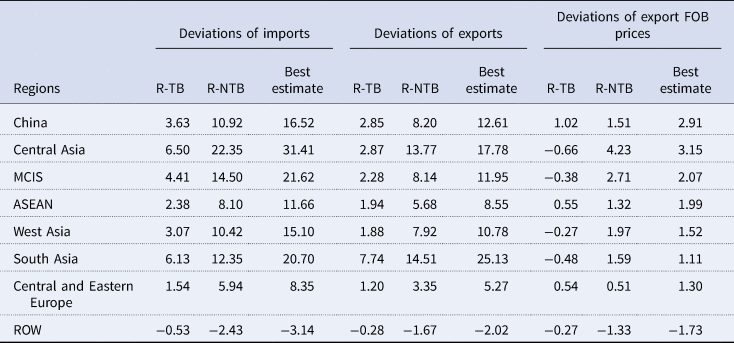
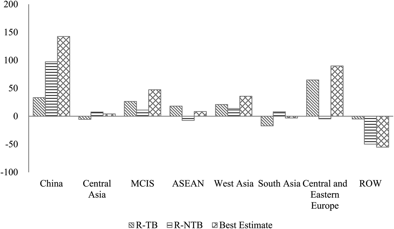
In the main text, all the scenarios include the joint impact of reduced tariff barriers (TB) and non-tariff barriers (NTB). In this appendix, we examine the impact if only one of the reduced TB and NTB is considered in the ‘best estimate’ scenario. Hence, two additional scenarios are introduced: one reducing TB only (R-TB) and the other reducing NTB only (R-NTB). Both scenarios are compared with the Reference Scenario to obtain their impacts on international trade and agricultural GVC positions. If only the reduced TBs are considered in the R-TB scenario, the imports and exports in the BR countries increase to a certain extent, but the increases are always less than the increases when the NTBs alone are considered, in the R-NTB scenario (Table A1). This indicates that NTB reductions have stronger impacts on international trade in our ‘best estimate’ scenario. Hence, the impacts on export prices in the ‘best estimate’ scenario are dominated by the reduced NTB in all regions. Generally, the joint impacts in the ‘best estimate’ scenario are greater than the simple sum of the impacts when only one of the trade barriers is reduced in the R-TB and R-NTB scenarios.
Comparison of various trade barrier reduction scenarios.%

Percentage changes in agricultural GVC position of three scenarios
Source: own calculation.