


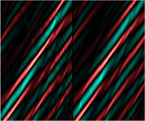



1. Introduction
The deterministic (i.e. phase-resolved) prediction of the incoming wave loads on marine structures represents one of the main challenges towards more efficient and safer offshore operations. The cost reduction of offshore wind through the extension of operational time windows for the installation/maintenance of offshore wind turbines, the gain in efficiency of marine energy devices through active control or the safety improvement of aircraft takeoffs/landings are only a few examples of domains that could benefit from the advance knowledge of wave-induced structure motions. Such predictions are performed by means of the calculation of the ocean surface evolution from the analysis of surrounding wave measurements. More specifically, they consist of three steps: (i) measuring some wave-related quantities, (ii) reconstructing the underlying wave field (i.e. extracting wave information from the measurements) and (iii) propagating the reconstructed wave field to the area of interest.
Regardless of their well-characterized properties and proven suitability for deterministic predictions, in situ wave measurements, such as made from wave buoys (e.g. Fisher, Thomson & Schwendeman Reference Fisher, Thomson and Schwendeman2021) or acoustic Doppler current profilers (Huchet et al. Reference Huchet, Babarit, Ducrozet, Gilloteaux and Ferrant2021), are not adaptable to predictions over a region in motion, such as around a ship with forward speed, due to the need to update the measured region according to the trajectory of the area of interest. In that case, measurements are typically performed from remote sensors mounted on a moving structure. Lidar cameras, for example, have recently been developed for the measurement of ocean surface displacements at a distance (Belmont et al. Reference Belmont, Horwood, Thurley and Baker2007; Kabel, Georgakis & Rod Zeeberg Reference Kabel, Georgakis and Rod Zeeberg2019), providing suitable data for wave prediction (Grilli, Guérin & Goldstein Reference Grilli, Guérin and Goldstein2011; Nouguier, Grilli & Guérin Reference Nouguier, Grilli and Guérin2014). Stereovideo systems are also able, through the mapping of the surface elevation, to give access to sufficient information for short-term forecasts (Mérigaud & Tona Reference Mérigaud and Tona2022). However, the real-time accessibility of wave data from stereo imaging is still constrained by the ‘significant computational time required to extract the three-dimensional elevation maps from a pair of images’ (Guimarães et al. Reference Guimarães, Ardhuin, Bergamasco, Leckler, Filipot, Shim, Dulov and Benetazzo2020), and subject to strong visibility limitations. Moreover, both lidar cameras and stereovideo systems are limited to measurement distances of  ${\sim }100$ m, restraining the prediction horizon to a few characteristic wave periods. Even if such prediction horizons are already valuable for applications such as optimal control of marine energy harvesting systems (e.g. Li et al. Reference Li, Weiss, Mueller, Townley and Belmont2012; Ma et al. Reference Ma, Sclavounos, Cross-Whiter and Arora2018), using sensors of higher measurement range could benefit a much larger variety of offshore operations.
The most commonly used remote sensors for the analysis of the ocean surface surrounding an offshore structure are non-coherent X-band marine radars, which are capable of measuring ocean surfaces over a much larger spatial domain, that is within a radius of  ${\sim }3$ km around the antenna. Surface wave identification from non-coherent radar data relies on the interpretation of the backscattered intensity which depends, through Bragg resonance, on the slope modulations of short ripples (gravity–capillary waves) by longer gravity waves (e.g. Alpers & Hasselmann Reference Alpers and Hasselmann1978; Alpers, Ross & Rufenach Reference Alpers, Ross and Rufenach1981). In addition, both the radars and the aforementioned remote sensing instruments located onboard a structure acquire data at grazing incidence. They are thus subject to wave shadowing that creates spatial gaps in the measured data sets. Two main approaches are used to retrieve the wave field from radar measurements (see the extensive review of Huang, Liu & Gill Reference Huang, Liu and Gill2017). The traditional method employs a semi-empirical modulation transfer function that relates the modal amplitudes of radar intensity to those of surface elevation in the frequency–wavenumber space (Young, Rosenthal & Ziemer Reference Young, Rosenthal and Ziemer1985; Nieto Borge et al. Reference Nieto Borge, Rodríguez, Hessner and González2004). Because this method identifies gravity wave components by choosing those which satisfy the linear dispersion relation, nonlinearities are disregarded. The alternative approach relies on the direct resolution of the modulation mechanisms of the radar backscattered intensity by assuming its proportionality to the surface slope. In that case, the linear wave theory is also assumed to facilitate data processing (Dankert & Rosenthal Reference Dankert and Rosenthal2004; Naaijen et al. Reference Naaijen, Van Oosten, Roozen and Van't Veer2018; Simpson et al. Reference Simpson, Haller, Walker, Lynett and Honegger2020).
Nevertheless, the linear wave assumptions have been shown to limit the prediction accuracy as the wave steepness and prediction horizon increase. To overcome this issue, second-order wave models that better represent the steep waves’ sharpness have been investigated (e.g. Hlophe et al. Reference Hlophe, Wolgamot, Kurniawan, Taylor, Orszaghova and Draper2021), albeit with a limited impact on the prediction accuracy because they miss nonlinear phase effects. Including corrections of the dispersion relation, appearing at third order, was shown to significantly help improve predictions (e.g. Blondel-Couprie, Bonnefoy & Ferrant Reference Blondel-Couprie, Bonnefoy and Ferrant2013; Desmars et al. Reference Desmars, Bonnefoy, Grilli, Ducrozet, Perignon, Guérin and Ferrant2020; Meisner et al. Reference Meisner, Galvagno, Andrade, Liberzon and Stuhlmeier2023), as well as using higher-order models based on the modified nonlinear Schrödinger equation (e.g. Trulsen Reference Trulsen2007; Simanesew et al. Reference Simanesew, Trulsen, Krogstad and Nieto Borge2017). For large wave steepness, the high-order spectral (HOS) method theoretically outperforms the aforementioned wave models (Klein et al. Reference Klein, Dudek, Clauss, Ehlers, Behrendt, Hoffmann and Onorato2020) by considering the evolution of the surface dynamics up to any arbitrary order of nonlinearity, with a relatively high computational efficiency. However, despite the rather large number of studies on HOS predictions, either based on sequential (Yoon, Kim & Choi Reference Yoon, Kim and Choi2016; Wang & Pan Reference Wang and Pan2021; Wang et al. Reference Wang, Zhang, Ma, Zhang, Li and Pan2022) or variational (Aragh & Nwogu Reference Aragh and Nwogu2008; Blondel, Bonnefoy & Ferrant Reference Blondel, Bonnefoy and Ferrant2010; Qi et al. Reference Qi, Wu, Liu, Kim and Yue2018a; Fujimoto & Waseda Reference Fujimoto and Waseda2020; Wu, Hao & Shen Reference Wu, Hao and Shen2022) assimilation strategies, the compatibility of the developed algorithms with remote measurement techniques must be further evaluated. Indeed, previous works suppose that the measurements (i) provide direct access to the surface elevation and (ii) are uniformly sampled in space and time. These two assumptions are not verified by non-coherent X-band radars in realistic conditions, for which the measurements take the form of return intensities subject to (a priori unknown) wave shadowing. Moreover, rather than a generally assumed sequence of spatial snapshots, radar data describe a space/time helix (Al-Ani et al. Reference Al-Ani, Christmas, Belmont, Duncan, Duncan and Ferrier2019). The available data are thus indirectly related to surface elevation and distributed in space and time in a non-trivial manner. It is expected that both of these features have an influence on the capacity of the methods to access information about the surface dynamics and predict the wave field.
It is thus proposed in the present paper to assess the impact of the modulation mechanisms that non-coherent radar measurements are subject to on the performance of linear, weakly nonlinear and highly nonlinear prediction algorithms. With this aim, three types of measurements (also called observations) with different levels of modulation are considered as input for the prediction of unidirectional wave fields with various wave steepness values. First, the observations correspond to surface elevations randomly distributed in space and time. Then, they are related to a radar model – the second type takes the shadowing modulation into account whereas the third one also includes the tilt modulation that makes the observed quantity mainly dependent on the surface slope. Regarding the prediction algorithms, two approaches are employed. The first one, based on the inversion of analytical wave models, extends the linear and weakly nonlinear approaches proposed by Desmars et al. (Reference Desmars, Bonnefoy, Grilli, Ducrozet, Perignon, Guérin and Ferrant2020) to radar observations and to the assessment of the reconstructed/predicted surface potential. The second one relies on the HOS method and extends the numerical basis of Desmars et al. (Reference Desmars, Hartmann, Behrendt, Klein and Hoffmann2022) to irregular waves and to radar observations. It follows a rather classical iterative optimization procedure that seeks the optimal variables (here, the HOS model parameters) by fitting the observations during a predefined time interval, such as done by variational assimilation, but presents some interesting numerical properties that are detailed later in the paper. By inter-comparison of the performance pertaining to each algorithm, the important hydrodynamic properties are highlighted for either the wave field reconstruction or prediction, which are independently evaluated. The case of regular waves is first considered to clearly identify the characteristics of each modelling method, then irregular waves are investigated. High-fidelity synthetic wave data are first used, before applying the methods to experimental wave tank data.
The paper is structured as follows. The theoretical aspects of non-coherent radar measurements, followed by those of the algorithms used for the wave field reconstructions, are presented in § 2. Section 3 details the numerical set-up that is used to evaluate the performance of the surface reconstructions and discusses the results. Likewise, § 4 describes the chosen configuration to study the methods’ prediction performance, before analysing the results. In § 5, the reconstruction/prediction methods are evaluated against wave tank experiments. Finally, § 6 presents the overall conclusions.
2. Theoretical background
Predicting surface waves deterministically implies going through three major steps. The first one is the measurement of the quantities that contain relevant information about the wave field for its prediction over a specific area of interest. The second step, referred to as surface reconstruction, is the extraction of wave information from the measurements to initialize the physical model that is used for the propagation of the wave field. The last step is the propagation of the reconstructed surface, giving access to the prediction. Considering that the ocean surface has to be predicted around a potentially mobile structure (e.g. a ship with forward speed), measurements are assumed to be done at a distance by a sensor mounted onboard the structure. The particularities of such remote measurements are detailed in this section, emphasizing their spatial non-uniformity and indirect relationship with surface fields. Then the investigated linear, weakly nonlinear and highly nonlinear methods for surface reconstruction are presented. For the sake of completeness, the theoretical aspects of the methods detailed in this paper describe the general case of directional wave fields, although the applications presented later are restricted to unidirectional waves.
2.1. Remote measurements
The prediction of the wave field around a mobile structure has to rely on measurements whose locations adapt to the structure's trajectory. X-band marine radars are considered in the subsequent developments. In contrast to coherent radars that can provide an estimation of the waves’ orbital velocities through the measurement of the Doppler frequency of the backscattered signal (e.g. Lyzenga et al. Reference Lyzenga, Nwogu, Beck, O'Brien, Johnson, de Paolo and Terrill2015; Støle-Hentschel et al. Reference Støle-Hentschel, Seemann, Nieto Borge and Trulsen2018), the considered sensor in the following applications is the much more common non-coherent radar, i.e. it only gives access to the backscattered signal intensity.
2.1.1. Marine radar model
Raw marine radar data are given in a polar coordinate system  $\left ( r,\beta,z \right )$. As depicted in figure 1,
 $r$ denotes the range distance, i.e. the distance between the antenna and the horizontal location of the ocean surface whose elevation is referred to as
 $\eta$, and
 $\beta$ is the azimuth angle of the radar look direction.
Geometrical parameters used for the representation of the shadowing and tilt modulations of marine radar beams.

The  $r$-axis is located at the mean surface level and points towards the radar look direction, while the
 $z$-axis is vertical and positive upward. The range resolution is constant and decided by the radar beam's pulse period, and the azimuth resolution is determined by the antenna beamwidth. For convenience, the ocean surface dynamics is described in a Cartesian system
 $\left ( x,y,z \right )=\left ( x_a+r\cos \beta,y_a+r\sin \beta,z \right )$, with
 $\left ( x_a,y_a \right )$ the horizontal coordinates of the radar antenna. Even though many studies consider radar data to be a sequence of instantaneous two-dimensional spatial snapshots (usually called ‘radar images’), the spatio-temporal distribution of the radar data actually describes a helix (Al-Ani et al. Reference Al-Ani, Christmas, Belmont, Duncan, Duncan and Ferrier2019). For unidirectional waves, however, the helix structure of the data does not apply, and they are modelled as a sequence of one-dimensional snapshots separated by a time step that corresponds to the antenna rotation period.
Among the different modulation mechanisms of the backscattered signal by the ocean surface, the shadowing and tilt modulations are considered prominent (e.g. Naaijen & Wijaya Reference Naaijen and Wijaya2014; Salcedo-Sanz et al. Reference Salcedo-Sanz, Nieto Borge, Carro-Calvo, Cuadra, Hessner and Alexandre2015) and their respective impact on wave prediction is studied in the present paper. The shadowing modulation describes the impact of obstructing waves in the region illuminated by the radar. Although the actual wave shadowing follows complex diffraction processes (Plant & Farquharson Reference Plant and Farquharson2012), it can be conveniently approximated by a geometrical approach (see figure 1): a point on the ocean surface is shadowed if a continuous straight line between that point and the radar antenna cannot be drawn without crossing the ocean surface. Practically, the shadowing modulation produces gaps in the spatial distribution of the radar measurements, as shown in figure 2(a). Because shadowing is stronger for larger angles of incidence  $\varTheta$ (defined in figure 1), the number and size of the gaps increase with the measurement distance and decrease with the sensor's height
 $z_a$. The tilt modulation modifies the intensity
 $\sigma$ of the backscattered signal according to the local angle of incidence of the radar beam on the surface. A geometrical approach can also be used to express this intensity (Nieto Borge et al. Reference Nieto Borge, Rodríguez, Hessner and González2004) and reads
 \begin{equation} \sigma=c_1\frac{\boldsymbol u\boldsymbol{\cdot}\boldsymbol n}{\left| \boldsymbol u \right|\left| \boldsymbol n \right|}+c_2, \end{equation}
where  $\boldsymbol n$ and
 $\boldsymbol u$ are the surface-normal and radar-beam vectors (see figure 1), respectively, and
 $\left | \boldsymbol u \right |$ (
 $\left | \boldsymbol n \right |$) denotes the Euclidean norm of
 $\boldsymbol u$ (
 $\boldsymbol n$). Here,
 $c_1$ is a scaling factor and
 $c_2$ an offset, which both depend on the calibration of the radar system and environmental conditions. The determination of these scaling coefficients is an active field of research. To name the most common methods, they can be found based on the signal-to-noise ratio of the backscattered signal (e.g. Lund et al. Reference Lund, Collins, Graber, Terrill and Herbers2014), on the shadowing (e.g. Ludeno & Serafino Reference Ludeno and Serafino2019) or statistical (e.g. Gangeskar Reference Gangeskar2000) properties of radar images or on an external reference measurement (e.g. Naaijen et al. Reference Naaijen, Van Oosten, Roozen and Van't Veer2018). The determination of these coefficients is outside of the scope of the present paper, hence they are here assumed to be known.
(a) Typical spatio-temporal distribution of observations from a marine radar scanning irregular unidirectional waves travelling from the left to the right. (b) Random spatio-temporal distribution using the same number of observations.

To study the influence of the modulation mechanisms on the wave prediction accuracy, surface reconstructions are systematically performed using three types of wave measurements, referred to as data types. Data type 1 corresponds to a set of randomly distributed surface elevations. Data type 2 refers to surface elevations that are subject to shadowing modulation. Both distributions are depicted in figure 2 with the same number of points. Finally, data type 3 designates radar intensities calculated from (2.1). All data types are summarized in table 1. The influence of the shadowing modulation or of the tilt modulation is studied by comparing results obtained with data types 1 and 2 or 2 and 3, respectively.
Definition of the three investigated types of observations.

2.1.2. Linear tilt modulation
The radar intensity model described by (2.1) is related to the surface elevation and slope in a nonlinear manner. Instead of inverting this nonlinear model during the surface reconstruction, a simplified linear model is used. Linearizing the intensity with respect to the surface slope and elevation (see details in Appendix A), (2.1) reduces to
 \begin{equation} \sigma=c_1\left( \cos\varTheta+\eta_r\sin\varTheta-\eta\frac{\sin^2\varTheta}{R} \right)+c_2, \end{equation}
where the index notation represents the corresponding derivative. Since the surface elevation in (2.2) is multiplied by the factor  $\sin ^2\varTheta /R\ll \sin \varTheta$, the dominant part of
 $\sigma$ is proportional to the surface radial slope
 $\eta _r$. Because the slope contains less information than the surface elevation (i.e. loss of an integration constant), using
 $\sigma$ as observations instead of
 $\eta$ is expected to impact the performance of the reconstruction methods.
It should be noted that the simplified approach leading to (2.1) and (2.2) does not consider the full complexity of non-coherent radar measurements, whose deterministic relationship with the surface elevation has yet to be empirically identified. Using real radar data instead of data type 3 is thus expected to have a negative effect on the surface reconstruction accuracy. Nevertheless, algorithms based on this model have been shown to yield sound results using field measurements (Dankert & Rosenthal Reference Dankert and Rosenthal2004; Naaijen et al. Reference Naaijen, Van Oosten, Roozen and Van't Veer2018).
2.2. Highly nonlinear surface reconstruction
The spatial and temporal scales of the problem allow us to use the potential flow theory, which assumes that the flow is irrotational and the fluid inviscid and incompressible. The flow is then described by the Laplace equation  ${\rm \Delta} \phi =0$ in the fluid domain, with
 $\phi$ the velocity potential, and by a non-penetration condition
 $\phi _z=0$ on the seabed, i.e. at
 $z=-h$ with
 $h$ the water depth. On the free surface, and using the surface velocity potential
 $\phi ^{s}\left ( x,y,t \right )=\phi \left ( x,y,z=\eta,t \right )$, the dynamic and kinematic free surface boundary conditions (FSBCs) yield (Zakharov Reference Zakharov1968)
 \begin{align} \left.\begin{aligned}
\phi^{s}_t&={-}g\eta-\tfrac{1}{2}\left|
\boldsymbol\nabla\phi^{s} \right|^2+\tfrac{1}{2}\left(
1+\left| \boldsymbol\nabla\eta \right|^2
\right)W,\\ \eta_t&=\left( 1+\left|
\boldsymbol\nabla\eta \right|^2
\right)W-\boldsymbol\nabla\phi^{s}\boldsymbol{\cdot}\boldsymbol\nabla\eta,
\end{aligned}\right\} \end{align}
where  $W=\phi _z\rvert _{z=\eta }$ is the vertical velocity on the free surface,
 $\boldsymbol \nabla =\left \{ \partial _x,\partial _y \right \}^{\textrm{T}}$ is the horizontal gradient,
 $t$ is the time and
 $g$ is the gravitational acceleration.
2.2.1. The HOS method
The HOS method is employed for both the generation of the reference ocean surface and its reconstruction. The core of the HOS method is the expression of the potential as a power series of  $\eta$ to a given arbitrary order
 $M\geq 1$, allowing the formulation of
 $W$ as a Taylor series involving
 $\eta$ and
 $\phi ^{s}$ (Dommermuth & Yue Reference Dommermuth and Yue1987; West et al. Reference West, Brueckner, Janda, Milder and Milton1987). Following the order-consistent formulation from West et al. (Reference West, Brueckner, Janda, Milder and Milton1987), the HOS FSBCs, expressed on the free surface, read
 \begin{align} \left.\begin{aligned}
\phi^{s}_t+g\eta&={-}\tfrac{1}{2}\left|
\boldsymbol\nabla\phi^{s} \right|^2+
\tfrac{1}{2}\left\lbrack \left( W^2 \right)_M+\left|
\boldsymbol\nabla\eta \right|^2\left( W^2 \right)_{M-2}
\right\rbrack,\\
\eta_t-\phi^{s}_z&=W_M^{nl}+\left| \boldsymbol\nabla\eta
\right|^2W_{M-2}-\boldsymbol\nabla\phi^{s}\boldsymbol{\cdot}\boldsymbol\nabla\eta,
\end{aligned}\right\} \end{align}
in which the linear terms have all been moved to the left-hand side, the subscript of the terms involving  $W$ denotes the order of expansion and
 $W_M^{nl}=W_M-W_1=W_M-\phi ^{s}_z$. The calculations are performed using a pseudo-spectral approach, in which the physical quantities are expressed by means of basis functions that satisfy the Laplace equation, the seabed condition and the horizontal boundary conditions of the computational domain. Here, the latter boundary conditions are assumed periodic so the velocity potential reads
 \begin{align} \phi\left( \boldsymbol
x,z,t \right)=\mbox{Re}\left\{
\sum_{i={-}\infty}^{+\infty}\sum_{j={-}\infty}^{+\infty}
{\mathsf{A}}^{\phi}_{ij}\left( t \right)\exp({\mathrm{i}\boldsymbol
k_{ij}\boldsymbol{\cdot}\boldsymbol x})
\frac{\cosh\left\lbrack \left| \boldsymbol k_{ij}
\right|\left( z+h \right) \right\rbrack}{\cosh\left( \left|
\boldsymbol k_{ij} \right|h \right)} \right\},
\end{align}
in which  ${\mathsf{A}}^{\phi }_{ij}\left ( t \right )$ are the complex spectral coordinates of
 $\phi$,
 $\boldsymbol x=\left \{ x,y \right \}^{\textrm{T}}$ and
 $\boldsymbol k_{ij}=\left \{ {k_x}_i,{k_y}_j \right \}^{\textrm{T}}$, where
 ${k_x}_i=i2{\rm \pi} /L_x$ and
 ${k_y}_j=j2{\rm \pi} /L_y$ with
 $L_x$ and
 $L_y$ the lengths of the computational domain along the
 $x$- and
 $y$-directions, respectively. The surface elevation has a similar expression without the
 $z$-dependent term. In practice, the sums in (2.5) are truncated to finite numbers
 $N_x$ and
 $N_y$. This approach allows the spatial-derivative operations to be performed efficiently due to the use of fast Fourier transforms (FFTs).
2.2.2. The HOS–observation coupling method
The highly nonlinear surface reconstruction is performed using the HOS–observation coupling method (HOS–OCM), which numerical basis follows that of Desmars et al. (Reference Desmars, Hartmann, Behrendt, Klein and Hoffmann2022). It consists of the inversion of a system that couples the equations describing the evolution of the ocean surface to a set of observation constraints having the form
 \begin{equation} \mathcal{M}\left( \phi^{s},\eta \right)=\zeta, \end{equation}
in which  $\zeta$ is the observed quantity (here, either the surface elevation or the radar intensity), and
 $\mathcal {M}$ is the observation-mapping function. This function both maps the physical quantities of interest (
 $\eta$ and
 $\phi ^{s}$) to the observation space and interpolates them to the spatio-temporal location of the observations. The wave equations are solved on a computational domain that has spatial lengths
 $L_x$ and
 $L_y$ and a duration
 $T_a$ (also called assimilation period). It is discretized with constant steps
 ${\rm \Delta} x$ and
 ${\rm \Delta} y$ in space and
 ${\rm \Delta} t$ in time (see figure 3). It contains
 $N_x$ and
 $N_y$ points along the spatial dimensions and
 $N_t$ points along the temporal dimension, leading to
 $N_p=N_xN_yN_t$ grid points in total. The reference point in space
 $\left ( x_0,y_0 \right )$ corresponds to the beginning of the computational domain, and the reference point in time
 $t_0$ corresponds to its first time (see figure 3).
Characteristics of the Cartesian computational domain used to perform the surface reconstruction with HOS–OCM.

The evolution equations (2.4) are coupled to (2.6) to form the inverse problem that is to be solved for the surface reconstruction. By recasting the resulting system in matrix form, it leads to
 \begin{align}
{{\boldsymbol{\mathsf{A}}}}\boldsymbol{\cdot}\left\lbrack
\begin{array}{@{}c@{}} \begin{matrix} \boldsymbol{\phi}^{s}
\end{matrix} \\ \hdashline[1pt/2pt] \begin{matrix}
\boldsymbol{\eta} \end{matrix} \end{array}
\right\rbrack=\boldsymbol b \iff \left\lbrack
\begin{array}{@{}c@{}} \begin{array}{c;{1pt/2pt}c} \begin{matrix}
{{\boldsymbol{\mathsf{A}}}}^{\partial_t} \end{matrix} &
\begin{matrix} g{{\boldsymbol{\mathsf{I}}}} \end{matrix}
\\ \hdashline[1pt/2pt] \begin{matrix}
-{{\boldsymbol{\mathsf{A}}}}^{\partial_z} \end{matrix} &
\begin{matrix} {{\boldsymbol{\mathsf{A}}}}^{\partial_t}
\end{matrix} \\ \hdashline[1pt/2pt] \end{array}\\
\begin{matrix} {{\boldsymbol{\mathsf{A}}}}^{\mathcal{M}}
\end{matrix} \end{array}
\right\rbrack\boldsymbol{\cdot} \left\lbrack
\begin{array}{@{}c@{}} \begin{matrix} \boldsymbol{\phi}^{s}
\end{matrix} \\ \hdashline[1pt/2pt] \begin{matrix}
\boldsymbol{\eta} \end{matrix} \end{array} \right\rbrack=
\left\lbrack \begin{array}{@{}c@{}} \begin{matrix}
\boldsymbol{b}^{d} \end{matrix} \\ \hdashline[1pt/2pt]
\begin{matrix} \boldsymbol{b}^{k} \end{matrix} \\
\hdashline[1pt/2pt] \begin{matrix} \boldsymbol{\zeta}
\end{matrix} \end{array} \right\rbrack,
\end{align}
where  ${{\boldsymbol{\mathsf{A}}}}^{\partial _t}$ corresponds to the time-derivative operator matrix,
 ${{\boldsymbol{\mathsf{A}}}}^{\partial _z}$ to the vertical-derivative operator matrix and
 ${{\boldsymbol{\mathsf{I}}}}$ to the identity matrix, all being
 $N_p$-by-
 $N_p$ matrices. The
 $N_o$-by-
 $2N_p$ (with
 $N_o$ the number of observations) matrix
 ${{\boldsymbol{\mathsf{A}}}}^{\mathcal {M}}$ corresponds to the observation-mapping function matrix. Vectors
 $\boldsymbol {\phi }^{s}$ and
 $\boldsymbol {\eta }$ contain the
 $N_p$ unknown grid values of surface potential and elevation, respectively. The right-hand side terms
 $\boldsymbol {b}^{d}$ and
 $\boldsymbol {b}^{k}$ correspond to the nonlinear parts of the dynamic and kinematic HOS FSBCs, respectively, and yield
 \begin{align} \boldsymbol{b}^{d}&={-}\frac{1}{2}\left\lbrack \left( {{\boldsymbol{\mathsf{A}}}}^{\partial_x}\boldsymbol{\cdot}\boldsymbol{\phi}^{s} \right)^2+ \left( {{\boldsymbol{\mathsf{A}}}}^{\partial_y}\boldsymbol{\cdot}\boldsymbol{\phi}^{s} \right)^2 \right\rbrack \nonumber\\ &\quad +\frac{1}{2}\left\{\left( \boldsymbol W^2 \right)_M+\left\lbrack \left( {{\boldsymbol{\mathsf{A}}}}^{\partial_x}\boldsymbol{\cdot} \boldsymbol{\eta} \right)^2+\left( {{\boldsymbol{\mathsf{A}}}}^{\partial_y}\boldsymbol{\cdot}\boldsymbol{\eta} \right)^2 \right\rbrack\left( \boldsymbol W^2 \right)_{M-2}\right\}, \end{align}
 \begin{align} \boldsymbol{b}^{k} &= \boldsymbol W_M^{nl}+\left\lbrack \left( {{\boldsymbol{\mathsf{A}}}}^{\partial_x}\boldsymbol{\cdot} \boldsymbol{\eta} \right)^2+\left( {{\boldsymbol{\mathsf{A}}}}^{\partial_y}\boldsymbol{\cdot}\boldsymbol{\eta} \right)^2 \right\rbrack\boldsymbol W_{M-2} \nonumber\\ &\quad -\left\lbrack \left( {{\boldsymbol{\mathsf{A}}}}^{\partial_x}\boldsymbol{\cdot}\boldsymbol{\eta} \right) \left( {{\boldsymbol{\mathsf{A}}}}^{\partial_x}\boldsymbol{\cdot}\boldsymbol{\phi}^{s} \right)+ \left( {{\boldsymbol{\mathsf{A}}}}^{\partial_y}\boldsymbol{\cdot}\boldsymbol{\eta} \right) \left( {{\boldsymbol{\mathsf{A}}}}^{\partial_y}\boldsymbol{\cdot}\boldsymbol{\phi}^{s} \right) \right\rbrack, \end{align}
where  ${{\boldsymbol{\mathsf{A}}}}^{\partial _x}$ and
 ${{\boldsymbol{\mathsf{A}}}}^{\partial _y}$ are the horizontal-derivative operator matrices, and
 $\boldsymbol W_M$ is a vector whose elements are the vertical velocities
 $W_M$. Finally, the vector
 $\boldsymbol \zeta$ contains the observations. When not specified by a distinctive mathematical symbol, operations on vectors are performed element-wise. The formulation of the matrices is detailed in Appendix B. The solution vectors
 $\boldsymbol {\phi }^{s}$ and
 $\boldsymbol \eta$ are found by minimizing, with the loose generalized minimum residual (LGMRES) algorithm (Baker, Jessup & Manteuffel Reference Baker, Jessup and Manteuffel2005), the norm of the residual function
 \begin{equation} \boldsymbol F={{\boldsymbol{\mathsf{A}}}}^{\textrm{T}}\boldsymbol{\cdot}{{\boldsymbol{\mathsf{A}}}}\boldsymbol{\cdot} \left\lbrack \begin{array}{@{}c@{}} \begin{matrix} \boldsymbol{\phi}^{s} \end{matrix} \\ \hdashline[1pt/2pt] \begin{matrix} \boldsymbol{\eta} \end{matrix} \end{array} \right\rbrack -{{\boldsymbol{\mathsf{A}}}}^{\textrm{T}}\boldsymbol{\cdot}\boldsymbol b. \end{equation}
For  $M=1$,
 $\boldsymbol {b}^{d}$ and
 $\boldsymbol {b}^{k}$ are full of zeros. For
 $M>1$, the solutions are obtained by inverting the system order by order, evaluating
 $\boldsymbol {b}^{d}$ and
 $\boldsymbol {b}^{k}$ from the lower-order solution. In the following, the first- and third-order solutions, referred to as HOSM1 and HOSM3, respectively, are investigated. The tolerances and restart parameter of the LGMRES iterative process have been fixed in such a way that they lead to converged results in terms of reconstruction accuracy.
Note that the computational cost of HOS–OCM is not related to that of a large dense matrix inversion as one might initially assume. Indeed, the chosen iterative solver for the minimization of (2.10) allows matrix-free calculations:  ${{\boldsymbol{\mathsf{A}}}}$ is not assembled, only matrix–vector products involving its submatrices are performed. These submatrices exhibit a high level of sparsity that leads them to have a product cost
 $O\left ( N_pN_s \right )$ for derivation or
 $O\left ( N_oN_s \right )$ for interpolation with
 $N_s\ll N_p$ the number of stencils to perform the considered operation. Matrix–vector products involving the spatial-derivative operator matrices
 ${{\boldsymbol{\mathsf{A}}}}^{\partial _{x,y,z}}$ are accelerated with FFTs resulting in a cost
 $O\left(N_p\log N_s\right)$. The transpose operations require the exact same computational effort. In fact, there is no additional cost coming from the matrix formulation of the problem, and the resulting number of operations is of the same order of magnitude as that of other HOS-based prediction algorithms relying on variational assimilation.
However, in contrast to variational approaches that control the HOS variables (namely the surface elevation and potential) at only one time step and propagate the solution over the assimilation period with a classical time-stepping procedure (typically using an explicit fourth-order Runge–Kutta scheme), HOS–OCM controls the variables at all time steps simultaneously. This formulation has two interesting numerical properties. First, no sequential time propagation of the solution is required, making possible the time parallelization of the model evaluation in the optimization process. This parallelization in time offers a greater impact on the computational time reduction than the parallelization in space whose effect is limited by the relatively small domain used for such surface reconstructions. Second, the embedded time integration of the wave equations has the properties of implicit schemes at no additional cost. More specifically, it exhibits high numerical stability – no evidence of instability was observed even for very large time steps – without the need to perform the additional system inversion that is required when the solution is sequentially propagated with implicit schemes. This gives flexibility in the choice of the time-step size, thus in the management of the computational time.
2.3. Parameterization of analytical wave models
The other investigated surface reconstruction method relies on the parameterization of analytical wave models. Besides a linear model that represents the water surface as the superposition of independent sine waves subject to the linear dispersion relation, two weakly nonlinear models are investigated. Based on a Lagrangian description of the surface motion, the improved choppy wave model catches nonlinear effects on both shape, i.e. sharper crests and flatter troughs, and phase, i.e. higher wave velocity (Guérin et al. Reference Guérin, Desmars, Grilli, Ducrozet, Perignon and Ferrant2019). In contrast, the second weakly nonlinear model considered here includes the correction of the dispersion relation pertaining to the improved choppy wave model, but no shape correction.
For these models, detailed below, the surface reconstruction is based on a least-squares algorithm that minimizes a quadratic cost function, similar to the approaches investigated by Desmars et al. (Reference Desmars, Bonnefoy, Grilli, Ducrozet, Perignon, Guérin and Ferrant2020). The cost function that is minimized reads
 \begin{equation} C=\tfrac{1}{2}\left| \boldsymbol\varLambda\left( \boldsymbol p \right)-\boldsymbol\varLambda^{o} \right|^2, \end{equation}
where the vector  $\boldsymbol \varLambda$ contains the wave model estimates of the observations,
 $\boldsymbol p$ contains the parameters of the wave model and
 $\boldsymbol \varLambda ^{o}$ contains either observed elevations (
 $\boldsymbol \eta ^{o}$) or radar intensities (
 $\boldsymbol \sigma ^{o}$) depending on the chosen data type. The optimal wave model parameters are obtained by applying the Levenberg–Marquardt algorithm (Moré Reference Moré1978) with explicit formulations of the Jacobian matrices that allow the procedure to be performed efficiently. The Jacobian matrices depend on the considered wave model and data type. Their expression for each configuration is given in Appendix C. In the rest of the paper, and in contrast to HOS–OCM, this reconstruction algorithm is referred to as the analytical-model-based method (AMBM).
2.3.1. Linear wave theory
The linear wave theory (LWT) gives the surface velocity potential and corresponding elevation according to
 $$\begin{gather} \phi_{LWT}^{s}\left( \boldsymbol x,t \right)=\sum_{n=1}^N\frac{\omega_n}{k_n}\left( a_n\sin\psi_n-b_n\cos\psi_n \right), \end{gather}$$
 $$\begin{gather}\eta_{LWT}\left( \boldsymbol x,t \right)=\sum_{n=1}^N\left( a_n\cos\psi_n+b_n\sin\psi_n \right), \end{gather}$$
in which  $\psi _n=\boldsymbol {k}_n\boldsymbol {\cdot }\boldsymbol x-\omega _n t$, with
 $\boldsymbol {k}_n=\left \{ {k_x}_n,{k_y}_n \right \}^{\textrm{T}}$, and
 $a_n$ and
 $b_n$ are the model parameters related to the amplitude and phase of
 $N$ individual wave components of predefined wavenumbers
 $k_n=\left | \boldsymbol {k}_n \right |$ related to angular frequencies
 $\omega _n$ through the linear dispersion relation
 $\omega _n^2=gk_n\tanh \left ( k_nh \right )$.
2.3.2. Improved choppy wave model
The improved choppy wave model (ICWM) was developed and characterized by Guérin et al. (Reference Guérin, Desmars, Grilli, Ducrozet, Perignon and Ferrant2019). It relies on the Lagrangian description of the water surface which allows the derivation, in a relatively simple mathematical form, of terms appearing at higher orders of expansion in wave steepness in the Eulerian formalism. Compared with the second-order Lagrangian solution (e.g. Nouguier, Chapron & Guérin Reference Nouguier, Chapron and Guérin2015), ICWM corrects the nonlinear effects affecting the waves’ velocity resulting in a more accurate description of the free surface kinematics. An Eulerian form of ICWM was used by Desmars et al. (Reference Desmars, Bonnefoy, Grilli, Ducrozet, Perignon, Guérin and Ferrant2020) to predict unidirectional waves and writes
 $$\begin{gather} \phi_{ICWM}^{s}\left( \boldsymbol x,t \right)=\sum_{n=1}^N\frac{\tilde\omega_n^{s}}{k_n} \left( a_n\sin\varPsi_n-b_n\cos\varPsi_n \right), \end{gather}$$
 $$\begin{gather}\eta_{ICWM}\left( \boldsymbol x,t \right)=\sum_{n=1}^N\left( a_n\cos\varPsi_n+b_n\sin\varPsi_n \right)+ \frac{1}{2}\sum_{n=1}^N\left( a_n^2+b_n^2 \right)k_n, \end{gather}$$
with
 \begin{align}
\left.\begin{aligned}
\displaystyle\varPsi_n&=\boldsymbol{k}_n\boldsymbol{\cdot}\left\lbrack
\boldsymbol x-\sum_{m=1}^N \dfrac{\boldsymbol
k_m}{k_m}\left({-}a_m\sin\psi_m^{nl}+b_m\cos\psi_m^{nl}
\right) \right\rbrack-\omega_n^{nl}t,\\
\psi_n^{nl}&=\boldsymbol{k}_n\boldsymbol{\cdot}\boldsymbol
x-\omega_n^{nl}t,\\
\displaystyle\omega_n^{nl}&=\omega_n+\frac{1}{2}\boldsymbol
k_n\boldsymbol{\cdot} \sum_{m=1}^N\left( a_m^2+b_m^2
\right)\omega_m\boldsymbol k_m,\\
\displaystyle\tilde\omega_n^{s}&=\omega_n-\frac{1}{2}\boldsymbol
k_n\boldsymbol{\cdot}\sum_{m=1}^N\left( a_m^2+b_m^2
\right)\omega_m\boldsymbol k_m. \end{aligned}\right\}
\end{align}
Note that the formulation of the surface potential of ICWM, not given yet in the literature, is discussed in Appendix D.
2.3.3. Linear wave theory with corrected dispersion relation
To quantify the importance of the correction of the dispersion relation only, a linear wave model that includes the correction of the dispersion relation pertaining to ICWM is also used. This model is referred to as LWT with corrected dispersion relation (LWT–CDR) and reads
 $$\begin{gather} \phi_{LC}^{s}\left( \boldsymbol x,t \right)=\sum_{n=1}^N\frac{\tilde\omega_n^{s}}{k_n} \left( a_n\sin\psi_n^{nl}-b_n\cos\psi_n^{nl} \right), \end{gather}$$
 $$\begin{gather}\eta_{LC}\left( \boldsymbol x,t \right)=\sum_{n=1}^N\left( a_n\cos\psi_n^{nl}+b_n\sin\psi_n^{nl} \right). \end{gather}$$
2.4. Numerical differences between HOS–OCM and AMBM
Throughout the paper, a systematic comparison of the reconstruction and prediction accuracy of each algorithm is performed. Leaving aside hydrodynamic considerations, this section aims at highlighting the numerical differences between HOS–OCM and AMBM to support the discussion of the results.
Even if both HOS–OCM and AMBM use least squares, through the minimization of  $\left | \boldsymbol F \right |$ (2.10) for HOS–OCM and of
 $C$ (2.11) for AMBM, a fundamental difference between the two methods is the nature of the control parameters of the minimization process. While they consist of the surface elevation and potential at the grid points for HOS–OCM, AMBM solves for the amplitude and phase of the wave components, and the surface fields are calculated from the model expressions after the minimization. This way, AMBM always gives a solution to the equations of the surface dynamics according to the considered wave model (i.e. LWT, LWT–CDR or ICWM). In contrast, the wave equations for HOS–OCM are seen as constraints that are not necessarily exactly verified by the solution. In addition, the wavenumbers of the wave components are not defined the same way for each method: they are implicitly defined by the grid size and resolution for HOS–OCM, and arbitrarily chosen for AMBM. To improve the comparability of the methods, the wave components of AMBM are chosen according to those implicitly defined by the computational grid of HOS–OCM. Although this might not correspond to the optimal choice of parameters for AMBM, convergence studies on the number of wave components have shown that, for both the synthetic and experimental configurations depicted in this paper (§§ 3 and 4, respectively), this choice leads to results that fairly represent the accuracy of the AMBM solver. Because numerical instabilities are arising for AMBM when very long modes are solved for, wave components whose wavenumber
 $k$ is lower than half the peak wavenumber
 $k_p$ of the observed wave field (i.e. the wavenumber of maximal energy) are not considered in the LWT, LWT–CDR and ICWM solutions.
2.5. Influence of the spatial periodicity assumption
Both HOS–OCM and AMBM (with similar wavenumbers to those of HOS–OCM, see the previous section) assume that the solution of the surface reconstruction problem is  $L_x$- and
 $L_y$-periodic, while the observations have no reason to exhibit spatial periodicity. Forcing the solution to match at the spatial boundaries of the reconstructed domain leads to discrepancies if no numerical treatment is employed. In the presented applications, the discrepancies induced by the periodicity assumption are restricted to a relatively small region on the domain boundaries. In consequence, no special treatment for the periodicity assumption was used a priori, the influence of these discrepancies on the results is reduced by evaluating the quality of the solution over a restricted domain that ends one peak wavelength (
 $\lambda _p=2{\rm \pi} /k_p$) away from each boundary. The size of the regions to be removed from the analysis was chosen for this study based on the evaluation of the actual results of the investigated cases. Changing the configuration, in particular the space and time extent of the observed domain, could modify the size of the impacted regions by the periodicity assumption.
3. Reconstructions
In this section, the numerical set-up to evaluate the accuracy of the reconstruction methods from synthetic surface observations is described before discussing the results.
3.1. Numerical set-up
Two unidirectional wave fields, made of regular and irregular waves that propagate along the positive  $x$-direction, aim at being reconstructed. Throughout the paper, the reconstruction and prediction configurations are set up with respect to the characteristics of the irregular wave field, even in the case of regular waves that is seen as a ‘simplified’ wave field of similar scales to help interpret the results. The irregular wave field is based on a JONSWAP energy distribution (Hasselmann et al. Reference Hasselmann1973) with a peak period
 $T_p=10$ s and a peak-enhancement factor of
 $3.3$. The wave height varies depending on the investigated wave steepness
 $H_s/\lambda _p$ (differing by a factor of
 ${\rm \pi}$ from the alternative steepness definition
 $\frac {1}{2} k_pH_s$), with
 $H_s$ the significant wave height defined as four times the standard deviation of the surface elevation. The regular wave field is defined from the peak wave characteristics of the irregular one, i.e. the period is
 $T=T_p$ and different values of wave steepness
 $H/\lambda$ (
 $=kA/{\rm \pi}$) are investigated, with
 $H=2A$ the wave height defined as the crest-to-trough height, and
 $\lambda =2{\rm \pi} /k=\lambda _p$ the wavelength. These wave fields, called reference wave fields and indicated by the superscript ‘r’ (e.g.
 $\eta ^{r}$), are generated using the HOS solver HOS-ocean (Ducrozet et al. Reference Ducrozet, Bonnefoy, Le Touzé and Ferrant2016) with a nonlinear order
 $M=4$, which provides converged results in terms of nonlinearity. The length of the domain is set to 32 peak wavelengths, deep water is assumed and a relaxation period
 $T_r$, such as described by Dommermuth (Reference Dommermuth2000), is used to smoothly turn the linearly initialized wave field into a fourth-order solution. A conservative simulation time of
 $2T_r$ is used before considering that the nonlinearities are fully developed and generating the synthetic observations. Regarding the spatial discretization, 32 points per peak wavelength are used, which ensures that the shortest wave sampled by the radar is properly resolved. This discretization, however, limits the steepness of the simulated irregular wave field to
 $H_s/\lambda _p\lesssim 3.2\,\%$ according to application ranges of highly nonlinear potential flow solvers (Ducrozet, Bonnefoy & Perignon Reference Ducrozet, Bonnefoy and Perignon2017).
To generate the radar observations, a virtual radar scans the surface and gives at every non-shadowed point one of the two observed quantities, that is either the surface elevation  $\boldsymbol \eta ^{o}=\eta _j^{r}$ (with
 $j=1,\ldots,N_o$) or the intensity
 $\boldsymbol \sigma ^{o}=\sigma _j^{r}$ according to (2.1). In the case the observations consist of radar intensities, the distances
 $\boldsymbol R^{o}=R_j$ and angles of incidence
 $\boldsymbol \varTheta ^{o}=\varTheta _j$ (see figure 1) are stored as well. In operating conditions,
 $R$ is approximated based on the time of flight of the radar beam, and
 $\varTheta$ is calculated based on the geometric relation
 $\varTheta =\cos ^{-1}\left ( z_a/R \right )$. Moreover, to decouple the effects of the wave shadowing (i.e. larger gaps in the spatial distribution of observations) from those of the wave steepness (i.e. stronger impact of the nonlinear wave physics) on the reconstruction accuracy for larger wave heights, the height of the radar antenna is made proportional to the wave height according to
 $z_a=8H_{\left ( s \right )}$ in the case of (ir)regular waves. This way, the shadowing properties are kept similar for all the investigated wave heights, and the observed differences in reconstruction accuracy between various steepness values are only related to hydrodynamic nonlinearities. The influence of the wave shadowing is quantified by comparing the results with those obtained with randomly distributed observations (i.e. data type 1 vs data type 2). Since the number of observations in the case of data type 1 is set similar to that obtained with the radar sampling of the surface (which includes wave shadowing), the overall density of observations is independent of the data type. Despite the unrealistic nature of the dependence between
 $z_a$ and the wave height, the factor of 8 already depicts a situation of strong shadowing (see figure 2a). The radar horizontal location is chosen such that it is facing the incoming waves and that there is a gap of
 $3\lambda _p\approx 470$ m between the radar and the reconstructed domain, i.e.
 $x_a=x_0+L_x+3\lambda _p$. The remaining radar characteristics are chosen according to Naaijen & Wijaya (Reference Naaijen and Wijaya2014), i.e. the range resolution is set to 7.5 m and the antenna rotation period, fixing the temporal resolution, to 1.5 s. Only the observations that fall into the reconstructed domain
 $\left \lbrack x_0,x_0+L_x \right \rbrack \times \left \lbrack t_0,t_0+T_a \right \rbrack$ are used for the reconstruction.
Concerning the computational domain of HOS–OCM, its spatial extent is  $L_x=12\lambda _p$ for a number of points
 $N_x=246$, leading to a resolution of
 ${\rm \Delta} x\approx \lambda _p/20.4\approx 7.6$ m. This is in agreement with the maximal spatial resolution of 7.5 m imposed by the observations in the case the ocean surface is sampled by the radar. The assimilation period is
 $T_a=3T_p$, which is long enough to give a converged reconstruction accuracy for the chosen measurement length, and the number of time steps is
 $N_t=48T_a/T_p=144$ (i.e.
 ${\rm \Delta} t\approx 0.21$ s).
3.2. Reconstruction accuracy quantification
For the quantification of the error between the reconstructed surface and the reference, the surface similarity parameter (SSP) is used. This indicator was developed by Perlin & Bustamante (Reference Perlin and Bustamante2016) and already used in the context of ocean wave prediction (e.g. Lünser et al. Reference Lünser, Hartmann, Desmars, Behrendt, Hoffmann and Klein2022). For the surface elevation, the SSP between the reconstructed field  $\eta$ and the reference
 $\eta ^{r}$ is formulated as
 \begin{equation} \mathrm{SSP}_\eta\left( t \right)=\frac{\displaystyle\left( \int\left| \mathcal{F}_\eta\left( k,t \right)- \mathcal{F}_{\eta^{r}}\left( k,t \right) \right|^2\,\mathrm{d} k \right)^{1/2}}{\displaystyle\left( \int\left| \mathcal{F}_\eta\left( k,t \right) \right|^2\,\mathrm{d} k \right)^{1/2}+\left( \int\left| \mathcal{F}_{\eta^{r}}\left( k,t \right) \right|^2\,\mathrm{d} k \right)^{1/2}}, \end{equation}
where  $\mathcal {F}_\eta$ denotes the spatial FFT of
 $\eta \left ( x,t \right )$ over the points of the computational domain of HOS–OCM. A similar expression holds for the surface potential error
 $\mathrm {SSP}_{\phi ^{s}}\left ( t \right )$. As mentioned in § 2.5, a restricted region that begins (ends) one peak wavelength after (before) the left (right) spatial boundary is selected for the quantification of the reconstruction accuracy to limit the influence of the periodicity assumption, i.e.
 $x\in \left \lbrack x_0+\lambda _p,x_0+L_x-\lambda _p \right \rbrack$. The value of the SSP is bounded by 0 and 1, meaning a perfect agreement or disagreement between the compared signals, respectively. Because the motion response of marine structures is most likely influenced by a limited frequency range, i.e. similar to a low-pass filter, the presented SSP calculation focuses on wavenumbers whose expected impact is significant. More specifically, this is done by retaining in (3.1) only the complex amplitudes
 $\mathcal {F}$ associated with wavenumbers lower than or equal to a cutoff value, here defined as
 $5k_p$. This choice is supported by the fact that the wave field evolution is mainly driven by wave components of wavenumber
 $k<5k_p$ (Ducrozet et al. Reference Ducrozet, Bonnefoy and Perignon2017). Moreover, to have an error indicator representing the global accuracy over the reconstructed domain, the time-averaged SSP between the two instants
 $t_0$ and
 $t_0+T_a$ is calculated. For the surface elevation, it reads
 \begin{equation} \overline{\mathrm{SSP}}_\eta=\frac{1}{T_a}\int_{t_0}^{t_0+T_a}\mathrm{SSP}_\eta\left( t \right)\,\mathrm{d} t. \end{equation}
An expression similar to (3.2) is used to quantify  $\overline {\mathrm {SSP}}_{\phi ^{s}}$. In the case of irregular waves, the SSP values are averaged over 200 wave field realizations with different sets of randomly chosen initial wave phases.
3.3. Reconstruction results
In this section, the ability of HOS–OCM and AMBM to accurately reconstruct the observed wave field is studied. First, regular waves are considered, leading to a clear distinction between the characteristics of each modelling method. Then irregular waves are reconstructed, showing the performance of the methods in more realistic wave conditions.
3.3.1. Regular waves
Reconstruction results for regular waves are presented in figure 4. They show that, for all data types, the reconstruction accuracy decreases for larger wave steepness when the wave model is not able to catch enough nonlinear features, consisting here of increasing the wave shape asymmetry and the wave velocity, the latter appearing from the third order. The HOSM1 and LWT are fully linear and miss the aforementioned nonlinear effects, penalizing the reconstruction accuracy when the steepness increases. The trend followed by LWT–CDR is almost similar to that of LWT (and of HOSM1), showing that modelling the nonlinear correction of the wave velocity is not enough to improve the reconstruction significantly. However, the influence of the wave velocity having linear and quadratic dependencies on the simulation time and wave steepness, respectively, means that the nonlinear correction of LWT–CDR is expected to be more impactful for longer assimilation period  $T_a$ and larger steepness. In contrast, the accuracy is very high for HOSM3 and ICWM, and barely affected by the steepness variation. This is because both models include all the nonlinear effects associated with regular waves up to the third order. As seen from the slightly lower accuracy obtained with data type 2 compared with data type 1, the wave shadowing effect, which tends to concentrate the discrepancies at the non-visible parts of the waves (e.g. troughs), has a limited impact. Using observations of radar intensity (data type 3) instead of elevation (data type 2) has a small influence as well, which validates that both HOS–OCM and AMBM can extract correct information about the surface dynamics from elevation or slope samples. In the case of data type 3, the fact that the accuracy of HOS–OCM is generally a little lower than that of AMBM most likely comes from the numerical differences detailed in § 2.4 between the two methods. In particular, performing the reconstruction from radar intensities instead of elevations might affect the relative weight of the HOS equations (2.4) with respect to the observation-mapping function in the minimized residual (2.10) of HOS–OCM, resulting in a lower accuracy. A penalty approach (e.g. Nocedal & Wright Reference Nocedal and Wright1999) could be employed to investigate the effect of the wave model enforcement (i.e. forcing the solution to strictly satisfy the HOS equations) on the reconstructed surface. Nevertheless, the SSP values remain below 0.05 in all configurations, and almost the same results are obtained for the surface potential.
Reconstruction accuracy for the regular wave field as a function of the steepness  $H/\lambda$ for HOSM1 (- -
 $\bullet$- -), HOSM3 (—
 $\bullet$—), LWT (- -
 $\triangle$- -, red), LWT–CDR (
 $\cdots \triangle \cdots $, red) and ICWM (–
 $\cdot \triangle$–
 $\cdot$, red). Results using data type (a,d) 1, (b,e) 2 and (c, f) 3 are presented (see table 1 for definitions).

Reconstruction of regular waves of larger steepness (up to  $H/\lambda \sim 10\,\%$) have been performed and provide results that are in line with the physical properties of the wave models, i.e. similar accuracy between HOSM3 and ICWM and progressive distinction between LWT and LWT–CDR for increasing steepness. For the very steep cases, however, the reference data generation, surface reconstruction and surface prediction procedures had to be slightly adapted to prevent various numerical perturbations from appearing, and whose study is left out of this paper for the sake of brevity.
3.3.2. Irregular waves
Reconstruction results for irregular waves are presented in figure 5. As expected, and similar to the case of regular waves, the lower-order models are less accurate, and the SSP values increase for larger wave steepness. However, larger SSP values than those of the regular waves are found, which can be explained by the increased complexity resulting from the interaction phenomena between waves of different scales. This is especially clear when the reconstruction relies on slope information (i.e. data type 3) for which the accuracy strongly depends on the correct resolution of the modulation of short waves by long waves, making the whole range of wave scales important to resolve. In contrast, mainly the waves of high amplitude (localized around the peak of the energy spectrum) influence the correct extraction of wave information from the observations when they consist of surface elevations (i.e. data types 1 and 2), simplifying the reconstruction. Radar intensities are also harder to use for surface reconstruction because they contain less information about the wave field than surface elevations, as explained in § 2.1.2. Regarding the linear approaches, HOSM1 systematically leads to a higher accuracy than LWT for data types 1 and 2, and to a significantly lower accuracy for data type 3. This could be explained, as for the regular waves, by the numerical differences between HOS–OCM and AMBM (see § 2.4). In combination with the numerical characteristics of HOS–OCM, the third-order modelling of HOSM3 gives the most accurate reconstructions for data types 1 and 2. As shown in figure 6(a) for data type 2, the improvement of HOSM3 over HOSM1 is mainly visible for large surface deformation. Without providing clear hints for interpretation, the discrepancies implied by the use of data type 3 in nonlinear reconstructions of the same surface can be spotted in figure 6(b). In general, the SSP values for the surface potential are a bit larger than for the surface elevation, which could come from the fact that, for all data types, the observations are related to the surface elevation but not directly to the surface potential. The potential is calculated from the wave model only, leading its reconstruction error to be slightly higher than that of the elevation.
Reconstruction accuracy for the irregular wave field as a function of the steepness  $H_s/\lambda _p$ for HOSM1 (- -
 $\bullet$- -), HOSM3 (—
 $\bullet$—), LWT (- -
 $\triangle$- -, red), LWT–CDR (
 $\cdots \triangle \cdots$, red) and ICWM (–
 $\cdot \triangle$–
 $\cdot$, red). Results using data type (a,d) 1, (b,e) 2 and (c, f) 3 are presented (see table 1 for definitions). The shaded areas show the standard deviation for HOSM3 and ICWM for the 200 wave field realizations.

Reconstructed surface elevation of irregular waves of steepness  $H_s/\lambda _p\approx 3.2\,\%$ at time
 $t_0+T_a$ using observations subject to wave shadowing and that consist of (a) surface elevations (i.e. data type 2) and (b) radar intensities (i.e. data type 3). Comparison of the reference surface (——, green) with HOSM1 (- - - -,
 $\mathrm {SSP}_\eta \approx 0.078$), HOSM3 (——,
 $\mathrm {SSP}_\eta \approx 0.024$ (a) and 0.076 (b)) and ICWM (–
 $\cdot$–
 $\cdot$, red,
 $\mathrm {SSP}_\eta \approx 0.062$).

4. Predictions
After investigating the performance of the methods for surface reconstruction, this section focuses on quantifying the accuracy that can be obtained by propagating the reconstructed solutions in view of predictions.
4.1. Definition of the prediction domain
The prediction accuracy is quantified over the theoretically accessible prediction zone corresponding to the spatio-temporal domain within which pieces of information about the reconstructed wave components, travelling at the group velocity  $c_g=\partial \omega /\partial k$, overlap (e.g. Naaijen, Trulsen & Blondel-Couprie Reference Naaijen, Trulsen and Blondel-Couprie2014; Qi et al. Reference Qi, Wu, Liu and Yue2018b). In practice, the boundaries of the prediction zone are defined by considering that the wave field can be accurately described by a finite frequency bandwidth containing the most energetic wave components. Here, similar to Desmars et al. (Reference Desmars, Bonnefoy, Grilli, Ducrozet, Perignon, Guérin and Ferrant2020) and Huchet et al. (Reference Huchet, Babarit, Ducrozet, Gilloteaux and Ferrant2021), cutoff angular frequencies
 $\omega _\ell$ and
 $\omega _h$ (with
 $\omega _\ell <\omega _h$) are selected such that
 $E\left ( \omega _\ell \right )=E\left ( \omega _h \right )=0.05E\left ( \omega _p \right )$, with
 $E\left ( \omega \right )$ the wave energy spectrum of the irregular wave field and
 $\omega _p=2{\rm \pi} /T_p$. These angular frequencies give the highest and lowest group velocities of the wave components of interest that define the prediction zone boundaries. Because it is supposed that the radar is mounted close to the location where the waves have to be anticipated, the target location for prediction is the radar location
 $x_a$ and the predicted surface is evaluated as a time series. Also, to maximize the prediction horizon, the last reconstructed solution (i.e. at
 $t=t_0+T_a$) is taken as the initial condition for the propagation. Finally, since the solution is considered valid over a restricted domain due to the spatial periodicity assumption (see § 2.5), the prediction zone is determined by neglecting information out of
 $\left \lbrack x_0-\lambda _p,x_0+L_x+\lambda _p \right \rbrack$. In consequence, a future time
 $t$ is included in the prediction zone at
 $x_a$ if it is part of the interval
 $\left \lbrack t_h,t_\ell \right \rbrack$ with
 $$\begin{gather} t_h=t_0+T_a+\frac{x_a-\left( x_0+L_x-\lambda_p \right)}{{c_g}_h}, \end{gather}$$
 $$\begin{gather}t_\ell=t_0+T_a+\frac{x_a-\left( x_0+\lambda_p \right)}{{c_g}_\ell}, \end{gather}$$
and the group velocities are calculated using the linear dispersion relation, i.e.  ${{c_g}=\frac {1}{2}\omega /k\left \lbrack 1+2kh/\sinh \left ( 2kh \right ) \right \rbrack}$, which already gives a good estimation of the extent of the prediction zone compared with a higher-order formulation of the dispersion relation (Qi et al. Reference Qi, Wu, Liu, Kim and Yue2018a). Figure 7 shows the geometrical interpretation of the prediction zone definition. In the depicted configuration, the obtained limits of the prediction horizon lead to
 $t_h-\left ( t_0+T_a \right )\approx 14T_p$ and
 $t_\ell -t_h\approx 6T_p$.
Definition of the theoretically accessible prediction zone from information contained in the reconstructed solution at  $t=t_0+T_a$.

4.2. Numerical aspects of the prediction using HOS–OCM
While the analytical models can be propagated in space and time without requiring any special numerical treatment, the HOS solutions from HOS–OCM need a fixed, periodic spatial domain to be propagated over. Here, the propagation of the HOS solutions is done as follows. First, the spatial computational domain of HOS–OCM is extended to include the location of the prediction  $x_a$. This domain is set similarly to that used for the generation of the reference surface described in § 3.1, and it is used to express the reconstructed solution at
 $t=t_0+T_a$ with zeros for
 $x\notin \left \lbrack x_0,x_0+L_x \right \rbrack$. The prediction is thus based on the propagation of the reconstructed solution obtained at the end of the assimilation period. Second, to avoid discontinuities, the solution is made smoothly go to zero at both ends of the reconstructed domain. More specifically, the surface fields
 $\eta$ and
 $\phi ^{s}$ are multiplied by the third-order polynomial
 \begin{equation}
f_s\left( x \right)=\begin{cases} \left\lbrack
\dfrac{x-\left( x_0-\lambda_p \right)}{\lambda_p}
\right\rbrack^2 \left\{ 3-2\left\lbrack \dfrac{x-\left(
x_0-\lambda_p \right)}{\lambda_p} \right\rbrack \right\}, &
\text{if }x\in\left\lbrack x_0-\lambda_p,x_0
\right\rbrack,\\ 1, & \text{if }x\in\left\lbrack
x_0,x_0+L_x \right\rbrack,\\ 1-\left\lbrack \dfrac{x-\left(
x_0+L_x \right)}{\lambda_p} \right\rbrack^2 \left\{
3-2\left\lbrack \dfrac{x-\left( x_0+L_x \right)}{\lambda_p}
\right\rbrack \right\}, \\
\quad \text{if }x\in\left\lbrack
x_0+L_x,x_0+L_x+\lambda_p \right\rbrack. \end{cases}
\end{equation}
Finally, the HOS-ocean solver is used for the forward propagation of the solution with an order of nonlinearity  $M$ matching that used for the reconstruction, i.e. either 1 or 3.
As described in § 4.1, even if the initial surface is perfectly known over a limited spatial domain, the dispersion of wave information during the surface propagation automatically prevents the prediction at a further point in space from perfectly matching the true solution. The accuracy of such a prediction depends on the amount of truncated energy by the cutoff frequencies defining the extent of the prediction zone, and a perfect prediction remains out of reach even with a perfectly reconstructed surface. Consequently, the optimal prediction accuracy can be quantified by applying the propagation procedure described above (although with  $M=4$) to the reference solution and comparing the obtained prediction with the normally propagated reference solution. The determination of this error is done in the following for the case of irregular waves and indicates how far the accuracy obtained with the investigated prediction algorithms is from the best achievable one. This optimal prediction accuracy quantification does not apply to regular wave fields because they are not subject to wave dispersion.
Because propagating a solution which boundaries have been smoothed down to zero potentially introduces non-physical artefacts in the simulation, the spectra of the reference prediction and that of the optimal prediction have been compared. This comparison showed that no artefact appears in the solution subject to the described smoothing process.
4.3. Prediction accuracy quantification
The SSP is used again to quantify the accuracy of the predicted surface elevation and potential. Because the comparison with the reference surface relies on time series, its formulation is different from (3.1) and follows
 \begin{equation}
\widetilde{\mathrm{SSP}}_\eta=\frac{\displaystyle\left(
\int\left| \mathcal{F}_\eta \left(\,f
\right)-\mathcal{F}_{\eta^{r}}\left(\,f \right)
\right|^2\,\mathrm{d} f \right)^{1/2}}{\displaystyle\left(
\int\left| \mathcal{F}_\eta \left(\,f \right)
\right|^2\,\mathrm{d} f \right)^{1/2}+\left( \int\left|
\mathcal{F}_{\eta^{r}}\left(\,f \right)
\right|^2\,\mathrm{d} f \right)^{1/2}},
\end{equation}
where  $\mathcal {F}_\eta$ denotes the temporal FFT of
 $\eta \left ( x_a,t \right )$ over the prediction period, i.e.
 $t\in \left \lbrack t_h,t_\ell \right \rbrack$, and
 $f$ is the frequency. A similar expression holds for the surface potential error
 $\widetilde {\mathrm {SSP}}_{\phi ^{s}}$. To only take into account the theoretically predictable wave components, the integral boundaries span the frequency range that is used to determine the extent of the prediction zone, i.e. the interval between
 $f_\ell =\omega _\ell /\left ( 2{\rm \pi} \right )$ and
 $f_h=\omega _h/\left ( 2{\rm \pi} \right )$.
4.4. Prediction results
Similar to the reconstruction, the ability of the different methods to predict the observed wave field is investigated for both regular and irregular wave fields.
4.4.1. Regular waves
Prediction results for regular waves are presented in figure 8, and unambiguously show the advantage of models that take into account the nonlinear correction of the wave velocity. Indeed, the accuracy decreases significantly with the wave steepness for both HOSM1 and LWT, while it remains very high for all the other models. This is in agreement with previous studies that compare the prediction performance of linear and nonlinear models and find that correct predictions of severe sea states can only be obtained with an accurate modelling of the wave velocity (e.g. Blondel-Couprie et al. Reference Blondel-Couprie, Bonnefoy and Ferrant2013; Desmars et al. Reference Desmars, Bonnefoy, Grilli, Ducrozet, Perignon, Guérin and Ferrant2020; Meisner et al. Reference Meisner, Galvagno, Andrade, Liberzon and Stuhlmeier2023). The effect of the nonlinear phase shift on the predicted surfaces is depicted in figure 9. The influence of both measurement modulation mechanisms, i.e. the wave shadowing effect and the use of radar intensities, on the prediction accuracy is very limited.
Prediction accuracy for the regular wave field as a function of the steepness  $H/\lambda$ for HOSM1 (- -
 $\bullet$- -), HOSM3 (—
 $\bullet$—), LWT (- -
 $\triangle$- -, red), LWT–CDR (
 $\cdots \triangle \cdots$, red) and ICWM (–
 $\cdot \triangle$–
 $\cdot$, red). Results using data type (a,d) 1, (b,e) 2 and (c, f) 3 are presented (see table 1 for definitions).

Predicted surface elevation of regular waves of steepness  $H/\lambda \approx 3.2\,\%$ at location
 $x_a$ from a reconstruction using observations subject to wave shadowing and that consist of radar intensities (i.e. data type 3). (a) Comparison of the reference surface (——, green) with LWT (- - - -, red,
 $\widetilde {\mathrm {SSP}}_\eta \approx 0.287$) and LWT–CDR (
 $\cdot \cdot \cdot \cdot \cdot \cdot \cdot \cdot$, red,
 $\widetilde {\mathrm {SSP}}_\eta \approx 0.049$). (b) Comparison of the reference surface with HOSM3 (——,
 $\widetilde {\mathrm {SSP}}_\eta \approx 0.014$) and ICWM (–
 $\cdot$–
 $\cdot$, red,
 $\widetilde {\mathrm {SSP}}_\eta \approx 0.023$).

4.4.2. Irregular waves
Prediction results for irregular waves are presented in figure 10. In this configuration, the benefit of HOSM3 is clear. Even if LWT–CDR and ICWM significantly improve the prediction compared with HOSM1 and LWT, the additional modelling effects included in HOSM3 substantially increase the accuracy. For data types 1 and 2, the results obtained with HOSM3 are satisfactory (see surface profiles in figure 11a), although there remains room to reach the optimal accuracy defined in § 4.2. Even for data type 3, for which HOSM3 leads to a relatively poor reconstruction compared with ICWM (see figure 5c, f), the propagation performance of HOSM3 leads to a prediction accuracy comparable to or even higher than that of ICWM for large wave steepness. Examples of nonlinear predictions using data type 3 are shown in figure 11(b) to illustrate the impact of the complete third-order modelling compared with ICWM. The nonlinear phase velocity correction of ICWM is independent of the properties of individual wave components, i.e. it acts as a global horizontal shift of the surface according to the sum of every wave component's Stokes drift (Guérin et al. Reference Guérin, Desmars, Grilli, Ducrozet, Perignon and Ferrant2019). In consequence, ICWM only models an ‘average’ nonlinear phase shift that is mainly driven by the most energetic wave components, and misses the frequency-dependent phase correction modelled by HOSM3. More specifically, compared with the modification of the dispersion relation due to third-order resonant effects (Longuet-Higgins & Phillips Reference Longuet-Higgins and Phillips1962), ICWM tends to overestimate (underestimate) the velocity correction of low-(high-)frequency wave components. It is also interesting to note that in the case of data type 3, ICWM gives better prediction results than LWT–CDR, while they are similar for data types 1 and 2. This emphasizes the need for accurate modelling of surface slopes when the observations are radar intensities.
Prediction accuracy for the irregular wave field as a function of the steepness  $H_s/\lambda _p$ for HOSM1 (- -
 $\bullet$- -), HOSM3 (—
 $\bullet$—), LWT (- -
 $\triangle$- -, red), LWT–CDR (
 $\cdots \triangle \cdots $, red) and ICWM (–
 $\cdot \triangle$–
 $\cdot$, red). The optimal accuracy defined in § 4.2 is also shown (— —). Results using data type (a,d) 1, (b,e) 2 and (c, f) 3 are presented (see table 1 for definitions). The shaded areas show the standard deviation for HOSM3 and ICWM for the 200 wave field realizations.

Predicted surface elevation of irregular waves of steepness  $H_s/\lambda _p\approx 3.2\,\%$ at location
 $x_a$ from a reconstruction using observations subject to wave shadowing and that consist of (a) surface elevations (i.e. data type 2) and (b) radar intensities (i.e. data type 3). Comparison of the reference surface (——, green) with HOSM1 (- - - -,
 $\widetilde {\mathrm {SSP}}_\eta \approx 0.498$), HOSM3 (——,
 $\widetilde {\mathrm {SSP}}_\eta \approx 0.036$ (a) and 0.062 (b)) and ICWM (–
 $\cdot$–
 $\cdot$, red,
 $\widetilde {\mathrm {SSP}}_\eta \approx 0.193$). The optimal prediction defined in § 4.2 is also shown in (a) (— —,
 $\widetilde {\mathrm {SSP}}_\eta \approx 0.010$).

5. Application to experimental data
In this section, the surface reconstruction/prediction algorithms are applied to real wave measurements from wave tank experiments. A description and characterization of the experimental data are provided by Clauss & Klein (Reference Clauss and Klein2011) and briefly recalled below.
5.1. Experimental set-up
The experimental campaign was carried out in the seakeeping wave tank of the Technical University of Berlin and aimed at studying the spatial development of an extreme wave. To this end, the New Year wave (also known as the Draupner wave) was reproduced at a scale 1:70 in the wave tank of length 120 m, width 8 m and depth 1 m. By generating the same unidirectional wave field multiple times and successively moving an array of wave gauges, a total number of 520 gauge measurements were performed with a spatial step of 0.1 m. In full scale (which will be used hereafter), the spatial extent of the measurements is 3633 m with a resolution of  ${\rm \Delta} x_e=7$ m, which is comparable to the spatial scale and resolution of radar measurements. The New Year wave appears at predefined target location and time, and the energy distribution of the surrounding wave field is assumed to be described by a JONSWAP spectrum with
 $T_p=16.7$ s,
 $H_s=11.92$ m and a peak-enhancement factor of 1. With a water depth of 70 m, it leads to a peak wavelength
 $\lambda _p\approx 364$ m.
This experimental configuration generalizes the applicability of the reconstruction/ prediction algorithms in three ways. First, the dimensionless wavenumber  $k_ph\approx 1.2$ makes the configuration fall into the finite water depth regime. Second, even if no specific characterization of the signal perturbations was done, the data generation process, based on the (generally non-perfect) repeatability of model tests (e.g. calibration and measurement inaccuracies with respect to vertical surface displacement but also horizontal position of the wave gauge array and distance in between) contaminates the space series of surface elevation with spurious fluctuations. Because the surface elevation was measured with an array of 13 wave gauges separated by an interval of
 $2{\rm \Delta} x_e$, that was translated by
 ${\rm \Delta} x_{e}$ between two successive wave generations, the main measurement repeatability errors take the form of localized fluctuations of wavelength
 $2{\rm \Delta} x_{e}$. The amplitude of these fluctuations depends on the repeatability between the two successive measurements for which the array of wave gauges was translated by
 ${\rm \Delta} x_{e}$, it is thus not constant all over the covered spatial domain. For instance, such fluctuations are clearly identifiable in figure 12 around
 $x-x_0=2800$ m. To check that the presented approaches are applicable to non-perfect input data, the raw experimental measurements are used without any preprocessing procedure to attenuate these perturbations. Finally, the wave field contains waves that are above the breaking limit, as reported by Clauss & Klein (Reference Clauss and Klein2011), leading breaking events to be included in the reference data. None of the reconstruction methods take into account wave breaking and, as explained in the next section, only the third-order HOS solution (HOSM3) models wave breaking during the surface propagation phase (i.e.
 $t>t_0+T_a$). Hence, the following results also inspect the capability of the reconstruction approaches to handle wave breaking in the input data, although they do not model it.
Time evolution of the spatial surface profiles, from the reconstruction ( $t-(t_0+T_a)\in [-50,0]$ s) to the prediction (
 $t-(t_0+T_a)>0$ s) using data type 1. The wave gauge measurements (——, green) are compared with the linear and nonlinear solutions of HOS–OCM, namely HOSM1 (- - - -) and HOSM3 (——). The solutions outside the theoretical prediction zone (
 $\cdots \cdots \cdot\cdot$, grey) are coloured in grey. The extreme wave appears at
 $t-(t_0+T_a)=40$ s.

5.2. Adaptation of the algorithms
Because (i) the observed waves are longer and steeper than in the numerical set-up and (ii) highly nonlinear potential flow solvers are subject to limitations in terms of wave steepness and space/modal discretization (Ducrozet et al. Reference Ducrozet, Bonnefoy and Perignon2017), the reconstruction algorithms are adapted as follows. First, the computational domain of HOS–OCM is extended and discretized according to its new dimension relative to  $\lambda _p$. Considering the limited spatial extent of the surface measurements, a length
 $L_x=2485\,{\rm m}\approx 6.8\lambda _p$ is chosen. By keeping the same number of points per peak wavelength, the grid is made of
 $N_x=140$ points. This extension also affects the choice of the wavenumbers
 $k_n$ of the wave components of the analytical models (see § 2.4). Note that the resulting spatial step
 ${\rm \Delta} x\approx 17.9$ m is longer than the wavelength of the measurement perturbations of wavelength
 $2{\rm \Delta} x_e=14\,{\rm m}$ described in the previous section. A similar assimilation period
 $T_a=3T_p$ (here
 ${\sim }50$ s) is used, and the number of time steps
 $N_t$ is still fixed to 48 per peak period. The location of the synthetic radar remains similar, i.e. approximately 470 m after the end of the computational domain. Then, due to the presence of breaking waves, the third-order HOS propagation of the reconstructed surface leads the surface elevation to be multi-valued if no energy is dissipated, making the simulation crash. In consequence, the propagation of the HOSM3 solution is performed by an in-house HOS engine that includes a wave breaking model as described by Wu (Reference Wu2004, § 4.4). It has been ensured, by comparing predicted surfaces for the steepest case presented in § 4.4.2, that the two employed HOS solvers lead to consistent results. The other wave models, whose numerical frameworks handle the propagation of very steep surfaces without crashing, are propagated without modelling any energy dissipation.
5.3. Results
The application of the algorithms to the experimental data is illustrated through one specific configuration chosen such that the New Year wave appears in the middle of the prediction zone 40 s after the surface reconstruction. Similar to the numerical investigation, the three data types described in § 2.1.1 are used as surface observations. The calculation of the prediction zone is similar to that described in § 4.1 with the characteristics of the wave field generated experimentally. Only the regions on the domain boundaries that are left out of the prediction zone due to the periodicity assumption (see § 2.5) are kept constant, i.e. approximately equal to 156 m. This choice follows the observation that the impact of the periodicity assumption on the accuracy of the reconstruction is very limited, and taking regions spanning one peak wavelength would be unnecessarily conservative.
The time evolutions of the reference and reconstructed space series of HOSM1 and HOSM3 using data type 1 are presented in figure 12, together with the propagated surfaces up to 100 s of prediction. Both solutions match well the reference surface in the reconstructed domain, that is for  $t-\left ( t_0+T_a \right )\in \left \lbrack -50,0 \right \rbrack$ s. The distinction between the linear and nonlinear solutions becomes stronger as time increases during the prediction, the linear solution being subject to an increasing phase delay and shape mismatch. In contrast, HOSM3 is able to predict the main features of the surface even after 100 s of prediction. It can also be noted from figure 12 that the definition of the theoretical prediction zone is conservative as the predicted surfaces also correlate, to a certain extent, with the reference outside the boundaries denoted by the dotted lines. A refined procedure for the determination of the actual prediction zone would be of practical interest to avoid underestimating the prediction horizon.
The accuracy is quantified through the calculation of  $\mathrm {SSP}_\eta$ (see § 3.2 for definition) over the reconstructed or predicted domain. In the latter case, the integral terms of (3.1) are bounded by
 $k_\ell$ and
 $k_h$ (calculated from
 $\omega _\ell$ and
 $\omega _h$, see § 4.1), the limiting wavenumbers of the waves included in the prediction zone. The results are presented in figure 13 for all wave models and data types. In agreement with the numerical results, HOSM3 and ICWM give the most accurate reconstructions/predictions for all data types, with a significant advantage for HOSM3. The linear solutions HOSM1 and LWT follow approximately the same trend and become rapidly incorrect as time increases. The LWT–CDR is consistent with the numerical results in the case of data types 1 and 2, i.e. its reconstruction accuracy is close to that of LWT, but gets closer to that of ICWM during the prediction phase. For data type 3, however, LWT–CDR fails to correctly reconstruct the surface with
 $\mathrm {SSP}_\eta >0.3$ for all the investigated times. The observed much harder convergence (i.e. need for much more iterations) of the weakly nonlinear AMBM solutions in the case of the experimental set-up compared with the numerical one could explain the depicted inconsistency in the results of LWT–CDR. The determination of the parameter responsible for this lower convergence rate, e.g. the presence of wave breaking events or measurement perturbations, would necessitate further investigations that are outside of the scope of this paper. In contrast, the convergence rate of HOS–OCM is similar in both numerical and experimental configurations.
Evolution of the spatial SSP of the surface elevation in time during the reconstruction ( $t-\left ( t_0+T_a \right )\leq 0$ s) and prediction (
 $t-\left ( t_0+T_a \right )>0$ s) periods for HOSM1 (- -
 $\bullet$- -), HOSM3 (—
 $\bullet$—), LWT (- -
 $\triangle$- -, red), LWT–CDR (
 $\cdots \triangle \cdots $, red) and ICWM (–
 $\cdot \triangle$–
 $\cdot$, red). Results using data type (a) 1, (b) 2 and (c) 3 are presented (see table 1 for definitions).

Finally, figure 14 gives a closer view of the New Year wave prediction for all wave models and data types. While all the other wave models miss the description of the surface elevation, HOSM3 is able to predict the correct phase and amplitude of the New Year wave for all data types. In addition to confirming that all the physics modelled at the third order is crucial for the correct description of steep wave fields (e.g. Lünser et al. Reference Lünser, Hartmann, Desmars, Behrendt, Hoffmann and Klein2022), this result suggests that a prediction system based on such a third-order surface dynamics would be enough for severe wave conditions.
Prediction of the New Year wave, 40 s after the reconstruction. The reference surface (——, green) is compared with the predicted solution obtained using data types 1 (——), 2 (- - - -) and 3 ( $\cdot \cdot \cdot \cdot \cdot \cdot \cdot\,\cdot$) for (a) HOSM1, (b) HOSM3, (c) LWT, (d) LWT–CDR and (e) ICWM.

6. Conclusions
The reconstruction and prediction accuracy of surface waves was investigated using observations representing different modulation mechanisms pertaining to remote measurements. Using a selection of methods that model different physical properties of the ocean surface, the impact of the wave shadowing and tilt modulations on the capacity of the prediction algorithms were highlighted. Reconstructing surfaces from observations subject to shadowing was found to have an impact limited to the non-visible regions. However, using radar intensities (assumed proportional to the surface slopes) instead of surface elevations affected the reconstruction more generally due to the indirect, more complex extraction of wave information from the measurements. It also brought to light some numerical properties of the reconstruction methods, HOS–OCM and AMBM, that influence their respective performances significantly. Still, both methods were able to predict waves in all configurations with an accuracy that depends on the limitations of the embedded physical model. It was shown that the accuracy of the surface reconstruction was mainly related to the correct modelling of the wave shape nonlinearities. In contrast, modelling the nonlinear correction of the dispersion relation had a marginal effect on the reconstruction accuracy but substantially helped improve the prediction. The third-order terms included in HOSM3 that model a frequency-dependent nonlinear wave phase correction (unlike ICWM) were shown to be crucial for the correct prediction of steep irregular waves. In addition, the application of the algorithms to data from wave tank experiments confirmed their suitability for non-perfect measurements, wave breaking and finite water depth. It demonstrated as well the feasibility of extreme wave predictions with HOSM3.
The encouraging results of HOS–OCM/HOSM3 call for further investigations on improving the compatibility of highly nonlinear wave models with reconstruction/ prediction algorithms from real radar measurements and other types of remotely acquired wave data. Though the presented study is restricted to unidirectional wave fields, the formalism has been developed to be applicable to directional waves, which will be the object of future studies. Relying on the explicit resolution of the wave equations also allows extending of the reconstruction to additional environmental parameters. Ongoing investigations are considering the inclusion of the current as an unknown of the surface reconstruction problem.
Acknowledgements
The authors would like to thank all the reviewers for their constructive comments.
Funding
This paper is published as a contribution to the joint research project EproBOSS. The authors wish to express their gratitude to the German Federal Ministry for Economic Affairs and Climate Action (BMWK) and Project Management Jülich (PtJ) for funding and supporting the project (M.K. and N.H., grant no. 03SX510A). Part of this work was funded by the Deutsche Forschungsgemeinschaft (DFG) (N.H., grant no. 277972093).
Declaration of interests
The authors report no conflict of interest.
Appendix A. Linearization of the radar intensity
Under the assumption that the main property affecting the radar backscatter is the local incidence angle of the radar beam on the surface, it is possible to express the intensity of the backscattered signal by the ocean surface as (Nieto Borge et al. Reference Nieto Borge, Rodríguez, Hessner and González2004)
 \begin{equation} \sigma=c_1\frac{\boldsymbol u\boldsymbol{\cdot}\boldsymbol n}{\left| \boldsymbol u \right|\left| \boldsymbol n \right|}+c_2, \end{equation}
with  $c_1$ is a scaling factor and
 $c_2$ an offset, and where
 $\boldsymbol n$ is the surface-normal vector and
 $\boldsymbol u$ the radar-beam vector, both depicted in § 2.1.1. These vectors are expressed as
 \begin{equation} \boldsymbol n= \left\lbrack \begin{array}{@{}c@{}} -\eta_x\\ -\eta_y\\ 1 \end{array} \right\rbrack= \left\lbrack \begin{array}{@{}c@{}} -\eta_r\cos\beta+\eta_\beta/r\sin\beta\\ -\eta_r\sin\beta-\eta_\beta/r\cos\beta\\ 1 \end{array} \right\rbrack, \end{equation}
and
 \begin{equation} \boldsymbol u= \left\lbrack \begin{array}{@{}c@{}} x_a-x\\ y_a-y\\ z_a-\eta \end{array} \right\rbrack= \left\lbrack \begin{array}{@{}c@{}} -r\cos\beta\\ -r\sin\beta\\ z_a-\eta \end{array} \right\rbrack, \end{equation}
from which is deduced
 \begin{equation} \frac{\boldsymbol u\boldsymbol{\cdot}\boldsymbol n}{\left| \boldsymbol u \right|\left| \boldsymbol n \right|} =\frac{r\eta_r+z_a-\eta}{\sqrt{r^2+\left( z_a-\eta \right)^2}\sqrt{\eta_r^2+\eta_\beta^2/r^2+1}}. \end{equation}
This leads to a nonlinear relation between  $\sigma$ and the surface elevation. By referring as
 $\epsilon$ to either the surface slopes
 $\eta _r$ and
 $\eta _\beta$ or elevation
 $\eta$, (A3) turns into
 \begin{equation} \frac{\boldsymbol u\boldsymbol{\cdot}\boldsymbol n}{\left| \boldsymbol u \right|\left| \boldsymbol n \right|}=\frac{r\eta_r}{R}+ \frac{z_a}{R}-\frac{r^2}{R^3}\eta+O\left( \epsilon^2 \right). \end{equation}
As a function of the nominal angle of incidence  $\varTheta$, it yields
 \begin{equation} \frac{\boldsymbol u\boldsymbol{\cdot}\boldsymbol n}{\left| \boldsymbol u \right|\left| \boldsymbol n \right|} =\cos\varTheta+\eta_r\sin\varTheta-\eta\frac{\sin^2\varTheta}{R}+O\left( \epsilon^2 \right). \end{equation}
The linearized solution of the backscattered radar intensity, assumed valid for the considered sea states, thus reads
 \begin{equation} \sigma=c_1\left( \cos\varTheta+\eta_r\sin\varTheta-\eta\frac{\sin^2\varTheta}{R} \right)+c_2. \end{equation}
Appendix B. Formulation of the HOS–OCM matrices
The formulation of the matrices used in HOS–OCM are described in this section.
B.1. In the HOS equations
The matrix  ${{\boldsymbol{\mathsf{A}}}}^{\partial _t}$ is defined according to a finite difference scheme using seven stencils (i.e. of sixth order of accuracy). A central scheme is used, except on the time boundaries of the grid where either forward or backward schemes are used instead. Spatial-derivative matrices
 ${{\boldsymbol{\mathsf{A}}}}^{\partial _x}$,
 ${{\boldsymbol{\mathsf{A}}}}^{\partial _y}$ and
 ${{\boldsymbol{\mathsf{A}}}}^{\partial ^\ell _z}$ are derived from the spectral definition of the derivative operators, i.e.
 $\partial _x\equiv \mathrm {i}k_x$,
 $\partial _y\equiv \mathrm {i}k_y$ and
 $\partial ^\ell _z\equiv \left | \boldsymbol k \right |^\ell$ (with a factor
 $\tanh \left ( \left | \boldsymbol k \right |h \right )$ for
 $\ell$ odd), respectively. The notation
 ${{\boldsymbol{\mathsf{A}}}}^{\partial _z}$ in (2.7) refers to
 ${{\boldsymbol{\mathsf{A}}}}^{\partial ^1_z}$. The vertical-velocity vector at order
 $M$ follows:
 \begin{equation} \boldsymbol W_M=\sum_{m=1}^M\boldsymbol W^{\left( m \right)}, \end{equation}
and each order is evaluated as
 \begin{equation} \boldsymbol W^{\left( m \right)}=\sum_{\ell=0}^{m-1}\frac{\boldsymbol{\eta}^\ell}{\ell !} {{\boldsymbol{\mathsf{A}}}}^{\partial^{\ell+1}_z}\boldsymbol{\cdot}\boldsymbol\phi^{\left( m-\ell \right)}. \end{equation}
The vector  $\boldsymbol \phi ^{\left ( m \right )}$ contains the approximation of the velocity potential at
 $z=0$ at order
 $m$ and is derived iteratively as
 $$\begin{gather} \boldsymbol\phi^{\left( 1 \right)}=\boldsymbol\phi^{s}, \end{gather}$$
 $$\begin{gather}\boldsymbol\phi^{\left( m \right)}={-}\sum_{\ell=1}^{m-1}\frac{\boldsymbol{\eta}^\ell}{\ell !}{{\boldsymbol{\mathsf{A}}}}^{\partial^\ell_z}\boldsymbol{\cdot}\boldsymbol\phi^{\left( m-\ell \right)},\quad m=2,\ldots,M. \end{gather}$$
To avoid spurious numerical results due to aliasing during the calculation of the products, a full dealiasing procedure is employed (e.g. Bonnefoy et al. Reference Bonnefoy, Ducrozet, Le Touzé and Ferrant2010). Finally, in order to prevent potential numerical instabilities from appearing in case of high wave steepness, high-frequency modal coefficients of the solution vectors  $\boldsymbol {\phi }^{s}$ and
 $\boldsymbol \eta$ that are used to construct the right-hand side terms
 $\boldsymbol {b}^{d}$ and
 $\boldsymbol {b}^{k}$, and of the right-hand side terms themselves, are damped according to an exponential filter before performing the system inversion.
B.2. Observation-mapping function
The observation-mapping function relates the quantities at the HOS grid points to the observations. It performs two basic operations, an interpolation (from the grid point locations to the observation locations, in both space and time) and a mapping (from the wave-quantities space to the observation space). More specifically, the latter operation is based on a function that expresses the measured quantity from the surface elevation and/or potential at the grid points. In the presented applications, the observations are related to the surface elevation only, as it is the case for considered wave sensors that give either  $\eta$ or
 $\sigma$ according to (2.2). The interpolation function takes the form of a
 $N_o$-by-
 $N_p$ matrix, denoted
 ${{\boldsymbol{\mathsf{A}}}}^{i}$, that uses Lagrange cubic polynomials. The mapping function depends on the considered observations, and its formulation is detailed below.
B.2.1. Mapping surface elevations
In the case the observations consist of surface elevations (i.e. data types 1 and 2), the constraint related to the observations is formulated as a simple interpolation following  $\boldsymbol \eta ^{o}={{\boldsymbol{\mathsf{A}}}}^{i}\boldsymbol {\cdot }\boldsymbol \eta$. To match the formalism of (2.7), this equality can be recast into
 \begin{equation} {{\boldsymbol{\mathsf{A}}}}^{\mathcal{M}}\boldsymbol{\cdot} \left\lbrack \begin{array}{@{}c@{}} \begin{matrix} \boldsymbol{\phi}^{s} \end{matrix} \\ \hdashline[1pt/2pt] \begin{matrix} \boldsymbol{\eta} \end{matrix} \end{array} \right\rbrack=\boldsymbol\zeta, \end{equation}
with  ${{\boldsymbol{\mathsf{A}}}}^{\mathcal {M}}=\left \{ {{\boldsymbol{\mathsf{O}}}},{{\boldsymbol{\mathsf{A}}}}^{i} \right \}$,
 $\boldsymbol \zeta =\boldsymbol \eta ^{o}$, and
 ${{\boldsymbol{\mathsf{O}}}}$ an
 $N_o$-by-
 $N_p$ matrix that is full of zeros.
B.2.2. Mapping radar intensities
In the case the observations consist of radar intensities, the constraint related to the observations is formulated based on the linear radar model (2.2). Consequently, the constraint related to the radar observations reads
 \begin{align} \boldsymbol\sigma^{o} &= c_1\left\{\cos\boldsymbol\varTheta^{o}+\left\lbrack \left( {{\boldsymbol{\mathsf{A}}}}^{i} \boldsymbol{\cdot}{{\boldsymbol{\mathsf{A}}}}^{\partial_x}\boldsymbol{\cdot}\boldsymbol\eta \right)\cos\boldsymbol\beta^{o}+ \left( {{\boldsymbol{\mathsf{A}}}}^{i}\boldsymbol{\cdot}{{\boldsymbol{\mathsf{A}}}}^{\partial_y} \boldsymbol{\cdot}\boldsymbol\eta \right)\sin\boldsymbol\beta^{o} \right\rbrack\sin\boldsymbol\varTheta^{o} \vphantom{\frac{\sin^2\boldsymbol\varTheta^{o}}{\boldsymbol R^{o}}}\right.\nonumber\\ &\quad \left.-\left( {{\boldsymbol{\mathsf{A}}}}^{i}\boldsymbol{\cdot}\boldsymbol\eta \right) \frac{\sin^2\boldsymbol\varTheta^{o}}{\boldsymbol R^{o}}\right\}+c_2\boldsymbol w, \end{align}
where vectors having the superscript  $^{o}$ contain quantities related to observations, namely the radar intensity
 $\sigma$, the angle of incidence
 $\varTheta$, the azimuth
 $\beta$ or the distance
 $R$ and
 $\boldsymbol w$ is a vector of length
 $N_o$ that is full of ones. The last equation is equivalent to
 \begin{equation} \frac{\boldsymbol\sigma^{o}}{\sin\boldsymbol\varTheta^{o}} = c_1\left\lbrack \frac{\cos\boldsymbol\varTheta^{o}}{\sin\boldsymbol\varTheta^{o}}+ \left( {{\boldsymbol{\mathsf{D}}}}^{c}\boldsymbol{\cdot}{{\boldsymbol{\mathsf{A}}}}^{i}\boldsymbol{\cdot} {{\boldsymbol{\mathsf{A}}}}^{\partial_x}+{{\boldsymbol{\mathsf{D}}}}^{s}\boldsymbol{\cdot} {{\boldsymbol{\mathsf{A}}}}^{i}\boldsymbol{\cdot}{{\boldsymbol{\mathsf{A}}}}^{\partial_y}- {{\boldsymbol{\mathsf{D}}}}^{e}\boldsymbol{\cdot}{{\boldsymbol{\mathsf{A}}}}^{i} \right)\boldsymbol{\cdot}\boldsymbol\eta \right\rbrack+ \frac{c_2}{\sin\boldsymbol\varTheta^{o}}, \end{equation}
in which  ${{\boldsymbol{\mathsf{D}}}}^{c}$,
 ${{\boldsymbol{\mathsf{D}}}}^{s}$ and
 ${{\boldsymbol{\mathsf{D}}}}^{e}$ are diagonal matrices built from vectors
 $\cos \boldsymbol \beta ^{o}$,
 $\sin \boldsymbol \beta ^{o}$ and
 $\sin \boldsymbol \varTheta ^{o}/\boldsymbol R^{o}$, respectively. To match the formalism of (2.7), equation (B7) is recast into
 \begin{equation} {{\boldsymbol{\mathsf{A}}}}^{\mathcal{M}}\boldsymbol{\cdot} \left\lbrack \begin{array}{@{}c@{}} \begin{matrix} \boldsymbol{\phi}^{s} \end{matrix} \\ \hdashline[1pt/2pt] \begin{matrix} \boldsymbol{\eta} \end{matrix} \end{array} \right\rbrack=\boldsymbol\zeta, \end{equation}
with
 \begin{equation} {{\boldsymbol{\mathsf{A}}}}^{\mathcal{M}}=\left\{ {{\boldsymbol{\mathsf{O}}}}, {{\boldsymbol{\mathsf{D}}}}^{c}\boldsymbol{\cdot}{{\boldsymbol{\mathsf{A}}}}^{i}\boldsymbol{\cdot} {{\boldsymbol{\mathsf{A}}}}^{\partial_x}+{{\boldsymbol{\mathsf{D}}}}^{s}\boldsymbol{\cdot} {{\boldsymbol{\mathsf{A}}}}^{i}\boldsymbol{\cdot}{{\boldsymbol{\mathsf{A}}}}^{\partial_y}- {{\boldsymbol{\mathsf{D}}}}^{e}\boldsymbol{\cdot}{{\boldsymbol{\mathsf{A}}}}^{i} \right\}, \end{equation}
and
 \begin{equation} \boldsymbol\zeta=\left( \frac{\boldsymbol\sigma^{o}}{c_1}-\frac{c_2}{c_1}\boldsymbol w-\cos \boldsymbol\varTheta^{o} \right)/\sin\boldsymbol\varTheta^{o}. \end{equation}
Appendix C. Expression of the analytical Jacobian matrices for the least-square problems of AMBM
In this section, the explicit formulation of the Jacobian matrix is given for all configurations of AMBM. Each one is characterized by a wave model (namely LWT, ICWM or LWT–CDR) and an observed quantity (i.e. surface elevation or radar intensity). For the considered wave models, the model parameters are always of the same form, i.e.  $\boldsymbol p=\left \{ a_1,\ldots,a_N,b_1,\ldots,b_N \right \}^{\textrm{T}}=\left \{ \boldsymbol v_a^{\textrm{T}},\boldsymbol v_b^{\textrm{T}} \right \}^{\textrm{T}}$, where
 $\boldsymbol v_a=a_n$ and
 $\boldsymbol v_b=b_n$ with
 $n=1,\ldots,N$ and
 $N$ the number of wave components. The matrix notation is used for conciseness and its similarity to the syntax of matrix-computation programming languages.
C.1. With elevation observations
Using the surface elevation as observed quantity, the cost function described by (2.11) writes
 \begin{equation} C=\tfrac{1}{2}\left| \boldsymbol\eta_{m}\left( \boldsymbol p \right)-\boldsymbol\eta^{o} \right|^2, \end{equation}
with  $\boldsymbol \eta _{m}$ the wave model evaluations of
 $\boldsymbol \eta ^{o}$. The corresponding
 $N_o$-by-
 $N$ Jacobian matrix is formed by the partial derivatives of every component of
 $\boldsymbol \eta _{m}$ with respect to every model parameter in
 $\boldsymbol p$. Explicit expressions are detailed below for LWT, ICWM and LWT–CDR.
C.1.1. Linear wave theory
The expression of the surface elevation according to LWT is given by (2.13), leading to the Jacobian matrix  ${{\boldsymbol{\mathsf{J}}}}_{\eta,LWT}=\left \{ {{\boldsymbol{\mathsf{B}}}}^{\textrm{T}}, {{\boldsymbol{\mathsf{C}}}}^{\textrm{T}} \right \}$ where
 ${{\boldsymbol{\mathsf{B}}}}=\cos \left ( \boldsymbol \kappa _x\otimes \boldsymbol x^{o}+\boldsymbol \kappa _y\otimes \boldsymbol y^{o}-\boldsymbol \omega \otimes \boldsymbol t^{o} \right )$ and
 ${{\boldsymbol{\mathsf{C}}}}=\sin \left ( \boldsymbol \kappa _x\otimes \boldsymbol x^{o}+\boldsymbol \kappa _y\otimes \boldsymbol y^{o}-\boldsymbol \omega \otimes \boldsymbol t^{o} \right )$ with
 $\otimes$ the outer product,
 $\boldsymbol \kappa _x={k_x}_n$,
 $\boldsymbol \kappa _y={k_y}_n$,
 $\boldsymbol \omega =\omega _n$, and
 $\boldsymbol x^{o}$,
 $\boldsymbol y^{o}$,
 $\boldsymbol t^{o}$ contain the
 $x$-,
 $y$-,
 $t$-coordinates of the observations, respectively.
C.1.2. Improved choppy wave model
The expression of the surface elevation according to ICWM is given by (2.15), leading to the Jacobian matrix  ${{\boldsymbol{\mathsf{J}}}}_{\eta,ICWM}=\left \{ {{\boldsymbol{\mathsf{E}}}}^{\textrm{T}}, {{\boldsymbol{\mathsf{F}}}}^{\textrm{T}} \right \}$ with
 $$\begin{gather} {{\boldsymbol{\mathsf{E}}}}={{\boldsymbol{\mathsf{G}}}}-\left( {{\boldsymbol{\mathsf{D}}}}^{a} \boldsymbol{\cdot}{{\boldsymbol{\mathsf{H}}}}-{{\boldsymbol{\mathsf{D}}}}^{b}\boldsymbol{\cdot} {{\boldsymbol{\mathsf{G}}}} \right)\odot{{\boldsymbol{\mathsf{K}}}}+ {{\boldsymbol{\mathsf{D}}}}^{ka}\boldsymbol{\cdot}{{\boldsymbol{\mathsf{U}}}}, \end{gather}$$
 $$\begin{gather}{{\boldsymbol{\mathsf{F}}}}={{\boldsymbol{\mathsf{H}}}}-\left( {{\boldsymbol{\mathsf{D}}}}^{a} \boldsymbol{\cdot}{{\boldsymbol{\mathsf{H}}}}-{{\boldsymbol{\mathsf{D}}}}^{b}\boldsymbol{\cdot} {{\boldsymbol{\mathsf{G}}}} \right)\odot{{\boldsymbol{\mathsf{L}}}}+{{\boldsymbol{\mathsf{D}}}}^{kb} \boldsymbol{\cdot}{{\boldsymbol{\mathsf{U}}}}, \end{gather}$$
where
 $$\begin{gather} {{\boldsymbol{\mathsf{K}}}}={{\boldsymbol{\mathsf{D}}}}^{k}\boldsymbol{\cdot} \left\lbrack {{\boldsymbol{\mathsf{C}}}}^{nl}-\left( {{\boldsymbol{\mathsf{D}}}}^{ka}\boldsymbol{\cdot} {{\boldsymbol{\mathsf{B}}}}^{nl}+{{\boldsymbol{\mathsf{D}}}}^{kb}\boldsymbol{\cdot} {{\boldsymbol{\mathsf{C}}}}^{nl}+{{\boldsymbol{\mathsf{U}}}} \right)\odot \left( \boldsymbol\kappa\boldsymbol\omega\boldsymbol v_a \right)\otimes\boldsymbol t^{o} \right\rbrack, \end{gather}$$
 $$\begin{gather}{{\boldsymbol{\mathsf{L}}}}={{\boldsymbol{\mathsf{D}}}}^{k}\boldsymbol{\cdot} \left\lbrack -{{\boldsymbol{\mathsf{B}}}}^{nl}-\left( {{\boldsymbol{\mathsf{D}}}}^{ka}\boldsymbol{\cdot} {{\boldsymbol{\mathsf{B}}}}^{nl}+{{\boldsymbol{\mathsf{D}}}}^{kb}\boldsymbol{\cdot} {{\boldsymbol{\mathsf{C}}}}^{nl}+{{\boldsymbol{\mathsf{U}}}} \right)\odot \left( \boldsymbol\kappa\boldsymbol\omega\boldsymbol v_b \right)\otimes\boldsymbol t^{o} \right\rbrack, \end{gather}$$
in which  $\odot$ denotes the element-wise matrix multiplication. Here,
 ${{\boldsymbol{\mathsf{D}}}}^{a}$,
 ${{\boldsymbol{\mathsf{D}}}}^{b}$,
 ${{\boldsymbol{\mathsf{D}}}}^{k}$,
 ${{\boldsymbol{\mathsf{D}}}}^{ka}$ and
 ${{\boldsymbol{\mathsf{D}}}}^{kb}$ are diagonal matrices built from vectors
 $\boldsymbol v_a$,
 $\boldsymbol v_b$,
 $\boldsymbol \kappa$,
 $\boldsymbol \kappa \boldsymbol v_a$ and
 $\boldsymbol \kappa \boldsymbol v_b$, respectively, where
 $\boldsymbol \kappa =k_n$.
 ${{\boldsymbol{\mathsf{B}}}}^{nl}=\cos \left ( \boldsymbol \kappa _x\otimes \boldsymbol x^{o}+\boldsymbol \kappa _y\otimes \boldsymbol y^{o}-\boldsymbol \omega ^{nl}\otimes \boldsymbol t^{o} \right )$ and
 ${{\boldsymbol{\mathsf{C}}}}^{nl}=\sin \left ( \boldsymbol \kappa _x\otimes \boldsymbol x^{o}+\boldsymbol \kappa _y\otimes \boldsymbol y^{o}-\boldsymbol \omega ^{nl}\otimes \boldsymbol t^{o} \right )$ are the nonlinear counterparts of
 ${{\boldsymbol{\mathsf{B}}}}$ and
 ${{\boldsymbol{\mathsf{C}}}}$ that include a correction of the dispersion relation, and
 $\boldsymbol \omega ^{nl}=\omega _n^{nl}$. Further,
 ${{\boldsymbol{\mathsf{U}}}}$ is an
 $N$-by-
 $N_o$ matrix that is full of ones. Finally,
 ${{\boldsymbol{\mathsf{G}}}}=\cos {{\boldsymbol{\mathsf{Q}}}}$ and
 ${{\boldsymbol{\mathsf{H}}}}=\sin {{\boldsymbol{\mathsf{Q}}}}$ with
 ${{\boldsymbol{\mathsf{Q}}}}$ a modified phase term defined by
 \begin{align} {{\boldsymbol{\mathsf{Q}}}} &= \boldsymbol\kappa_x\otimes \left\{ \boldsymbol x^{o}-\left\lbrack -\left( \frac{\boldsymbol\kappa_x\boldsymbol v_a}{\boldsymbol\kappa} \right)^{\textrm{T}} \boldsymbol{\cdot}{{\boldsymbol{\mathsf{C}}}}^{nl}+\left( \frac{\boldsymbol\kappa_x\boldsymbol v_b}{\boldsymbol\kappa} \right)^{\textrm{T}}\boldsymbol{\cdot} {{\boldsymbol{\mathsf{B}}}}^{nl} \right\rbrack \right\} \nonumber\\ &\quad +\boldsymbol\kappa_y\otimes\left\{ \boldsymbol y^{o}-\left\lbrack -\left( \frac{\boldsymbol\kappa_y\boldsymbol v_a}{\boldsymbol\kappa} \right)^{\textrm{T}} \boldsymbol{\cdot}{{\boldsymbol{\mathsf{C}}}}^{nl}+\left( \frac{\boldsymbol\kappa_y\boldsymbol v_b}{\boldsymbol\kappa} \right)^{\textrm{T}}\boldsymbol{\cdot} {{\boldsymbol{\mathsf{B}}}}^{nl} \right\rbrack \right\} \nonumber\\ &\quad -\boldsymbol\omega^{nl}\otimes\boldsymbol t^{o}. \end{align}
C.1.3. Linear wave theory with corrected dispersion relation
The expression of the surface elevation according to LWT–CDR is given by (2.18), leading to the Jacobian matrix  ${{\boldsymbol{\mathsf{J}}}}_{\eta,LC}=\left \{ {{\boldsymbol{\mathsf{M}}}}^{\textrm{T}}, {{\boldsymbol{\mathsf{N}}}}^{\textrm{T}} \right \}$ with
 $$\begin{gather} {{\boldsymbol{\mathsf{M}}}}={{\boldsymbol{\mathsf{B}}}}^{nl}+\left( {{\boldsymbol{\mathsf{D}}}}^{ka} \boldsymbol{\cdot}{{\boldsymbol{\mathsf{C}}}}^{nl}-{{\boldsymbol{\mathsf{D}}}}^{kb}\boldsymbol{\cdot} {{\boldsymbol{\mathsf{B}}}}^{nl} \right)\odot\left( \boldsymbol\kappa\boldsymbol\omega\boldsymbol v_a \right)\otimes\boldsymbol t^{o}, \end{gather}$$
 $$\begin{gather}{{\boldsymbol{\mathsf{N}}}}={{\boldsymbol{\mathsf{C}}}}^{nl}+\left( {{\boldsymbol{\mathsf{D}}}}^{ka} \boldsymbol{\cdot}{{\boldsymbol{\mathsf{C}}}}^{nl}-{{\boldsymbol{\mathsf{D}}}}^{kb}\boldsymbol{\cdot} {{\boldsymbol{\mathsf{B}}}}^{nl} \right)\odot\left( \boldsymbol\kappa\boldsymbol\omega\boldsymbol v_b \right)\otimes\boldsymbol t^{o}. \end{gather}$$
C.2. With radar intensity observations
Using the radar intensity as observed quantity, the cost function described by (2.11) writes
 \begin{equation} C=\tfrac{1}{2}\left| \boldsymbol\sigma_{m}\left( \boldsymbol p \right)-\boldsymbol\sigma^{o} \right|^2, \end{equation}
with  $\boldsymbol \sigma _{m}$ the wave model evaluations of
 $\boldsymbol \sigma ^{o}$. The corresponding
 $N_o$-by-
 $N$ Jacobian matrix is formed by the partial derivatives of every component of
 $\boldsymbol \sigma _{m}$ with respect to every model parameter in
 $\boldsymbol p$. Explicit expressions are detailed below for LWT, ICWM and LWT–CDR.
C.2.1. Linear wave theory
The formulation of the LWT radar intensity is obtained by inserting (2.13) into (2.2), which gives
 \begin{align} \sigma_{LWT}\left( \boldsymbol x,t \right) &= c_1\sin\varTheta\sum_{n=1}^{N} \left\{{-}a_n\left\lbrack \left( {k_x}_n\cos\beta+{k_y}_n\sin\beta \right)\sin\psi_n+\frac{\sin\varTheta}{R}\cos\psi_n \right\rbrack \right. \nonumber\\ &\quad \left.+ b_n\left\lbrack \left( {k_x}_n\cos\beta+{k_y}_n\sin\beta \right)\cos\psi_n-\frac{\sin\varTheta}{R}\sin\psi_n \right\rbrack\right\} \nonumber\\ &\quad + c_1\cos\varTheta+c_2. \end{align}
The corresponding Jacobian matrix is  ${{\boldsymbol{\mathsf{J}}}}_{\sigma,LWT}=\left \{ {{\boldsymbol{\mathsf{R}}}}^{\textrm{T}}, {{\boldsymbol{\mathsf{S}}}}^{\textrm{T}} \right \}$ with
 $$\begin{gather} {{\boldsymbol{\mathsf{R}}}}={-}\left( {{\boldsymbol{\mathsf{T}}}}\odot {{\boldsymbol{\mathsf{C}}}}+{{\boldsymbol{\mathsf{B}}}}\boldsymbol{\cdot} {{\boldsymbol{\mathsf{D}}}}^{e} \right)\boldsymbol{\cdot}{{\boldsymbol{\mathsf{D}}}}^{g}, \end{gather}$$
 $$\begin{gather}{{\boldsymbol{\mathsf{S}}}}=\left( {{\boldsymbol{\mathsf{T}}}}\odot {{\boldsymbol{\mathsf{B}}}}-{{\boldsymbol{\mathsf{C}}}}\boldsymbol{\cdot}{{\boldsymbol{\mathsf{D}}}}^{e} \right) \boldsymbol{\cdot}{{\boldsymbol{\mathsf{D}}}}^{g}, \end{gather}$$
in which  ${{\boldsymbol{\mathsf{T}}}}=\boldsymbol \kappa _x\otimes \cos \boldsymbol \beta ^{o}+\boldsymbol \kappa _y\otimes \sin \boldsymbol \beta ^{o}$, the definitions of
 $\boldsymbol \beta ^{o}$,
 $\boldsymbol \varTheta ^{o}$,
 $\boldsymbol w$ and
 ${{\boldsymbol{\mathsf{D}}}}^{e}$ follow from § B.2.2, and
 ${{\boldsymbol{\mathsf{D}}}}^{g}$ is a diagonal matrix built from the vector
 $c_1\sin \boldsymbol \varTheta ^{o}$.
C.2.2. Improved choppy wave model
The formulation of the ICWM radar intensity is obtained by inserting (2.15) into (2.2), which gives
 \begin{align} & \sigma_{ICWM}\left( \boldsymbol x,t \right) \nonumber\\ &\quad =c_1\sin\varTheta\sum_{n=1}^{N} \left[{-}a_n\left(\{[{k_x}_n(1-l)-{k_y}_nd]\cos\beta+[{k_y}_n\left( 1-q \right)-{k_x}_nd]\sin\beta\}\sin\varPsi_n \vphantom{\frac{\sin\varTheta}{R}}\right.\right. \nonumber\\ &\qquad \left.+\frac{\sin\varTheta}{R}\cos\varPsi_n\right) \nonumber\\ &\qquad +b_n\left(\{[{k_x}_n(1-l)-{k_y}_nd]\cos\beta+[{k_y}_n\left( 1-q \right)-{k_x}_nd]\sin\beta\}\cos\varPsi_n \vphantom{\frac{\sin\varTheta}{R}}\right. \nonumber\\ &\qquad \left.\left.-\frac{\sin\varTheta}{R}\sin\varPsi_n\right)- \frac{\sin\varTheta}{2R}\left(a_n^2+b_n^2\right)k_n\right]+c_1\cos\varTheta+c_2, \end{align}
with
 \begin{align} \left.\begin{aligned}
d&=\displaystyle\sum_{n=1}^N\frac{{k_x}_n{k_y}_n}{k_n}\left({-}a_n\cos\psi_n^{nl}-b_n\sin\psi_n^{nl}
\right),\\
l&=\displaystyle\sum_{n=1}^N\frac{{k_x}_n^2}{k_n}\left({-}a_n\cos\psi_n^{nl}-b_n\sin\psi_n^{nl}
\right),\\
q&=\displaystyle\sum_{n=1}^N\frac{{k_y}_n^2}{k_n}\left({-}a_n\cos\psi_n^{nl}-b_n\sin\psi_n^{nl}
\right). \end{aligned}\right\} \end{align}
The corresponding Jacobian matrix is  ${{\boldsymbol{\mathsf{J}}}}_{\sigma,ICWM}= \left \{ {{\boldsymbol{\mathsf{V}}}}^{\textrm{T}},{{\boldsymbol{\mathsf{W}}}}^{\textrm{T}} \right \}$ with
 \begin{align} {{\boldsymbol{\mathsf{V}}}} &= \left\{{{\boldsymbol{\mathsf{X}}}}\odot\left\lbrack {{\boldsymbol{\mathsf{H}}}}+ \left( {{\boldsymbol{\mathsf{D}}}}^{a}\boldsymbol{\cdot}{{\boldsymbol{\mathsf{G}}}}+ {{\boldsymbol{\mathsf{D}}}}^{b}\boldsymbol{\cdot}{{\boldsymbol{\mathsf{H}}}} \right)\odot{{\boldsymbol{\mathsf{K}}}} \right\rbrack \right.\nonumber\\ &\quad \left.-\left( {{\boldsymbol{\mathsf{D}}}}^{m}\boldsymbol{\cdot}{{\boldsymbol{\mathsf{M}}}}\boldsymbol{\cdot} {{\boldsymbol{\mathsf{D}}}}^{c} +{{\boldsymbol{\mathsf{D}}}}^{n}\boldsymbol{\cdot} {{\boldsymbol{\mathsf{M}}}}\boldsymbol{\cdot}{{\boldsymbol{\mathsf{D}}}}^{s} \right) \odot\left( {{\boldsymbol{\mathsf{D}}}}^{a}\boldsymbol{\cdot}{{\boldsymbol{\mathsf{H}}}}- {{\boldsymbol{\mathsf{D}}}}^{b}\boldsymbol{\cdot}{{\boldsymbol{\mathsf{G}}}} \right) -{{\boldsymbol{\mathsf{E}}}}\boldsymbol{\cdot}{{\boldsymbol{\mathsf{D}}}}^{e}\right\}\boldsymbol{\cdot} {{\boldsymbol{\mathsf{D}}}}^{g}, \end{align}
 \begin{align} {{\boldsymbol{\mathsf{W}}}} &= \left\{{{\boldsymbol{\mathsf{X}}}}\odot\left\lbrack -{{\boldsymbol{\mathsf{G}}}}+ \left( {{\boldsymbol{\mathsf{D}}}}^{a}\boldsymbol{\cdot}{{\boldsymbol{\mathsf{G}}}}+ {{\boldsymbol{\mathsf{D}}}}^{b}\boldsymbol{\cdot}{{\boldsymbol{\mathsf{H}}}} \right)\odot{{\boldsymbol{\mathsf{L}}}} \right\rbrack \right.\nonumber\\ &\quad \left.-\left( {{\boldsymbol{\mathsf{D}}}}^{m}\boldsymbol{\cdot} {{\boldsymbol{\mathsf{N}}}}\boldsymbol{\cdot}{{\boldsymbol{\mathsf{D}}}}^{c} + {{\boldsymbol{\mathsf{D}}}}^{n}\boldsymbol{\cdot}{{\boldsymbol{\mathsf{N}}}} \boldsymbol{\cdot}{{\boldsymbol{\mathsf{D}}}}^{s} \right)\odot\left( {{\boldsymbol{\mathsf{D}}}}^{a} \boldsymbol{\cdot}{{\boldsymbol{\mathsf{H}}}}-{{\boldsymbol{\mathsf{D}}}}^{b}\boldsymbol{\cdot} {{\boldsymbol{\mathsf{G}}}} \right)-{{\boldsymbol{\mathsf{F}}}}\boldsymbol{\cdot}{{\boldsymbol{\mathsf{D}}}}^{e}\right\} \boldsymbol{\cdot}{{\boldsymbol{\mathsf{D}}}}^{g}, \end{align}
in which  ${{\boldsymbol{\mathsf{X}}}}=-{{\boldsymbol{\mathsf{T}}}} +\boldsymbol \kappa _x\otimes \boldsymbol l\cos \boldsymbol \beta ^{o} +\boldsymbol \kappa _y\otimes \boldsymbol d\cos \boldsymbol \beta ^{o} +\boldsymbol \kappa _y\otimes \boldsymbol q\sin \boldsymbol \beta ^{o} +\boldsymbol \kappa _x\otimes \boldsymbol d\sin \boldsymbol \beta ^{o}$. Diagonal matrices
 ${{\boldsymbol{\mathsf{D}}}}^{m}$ and
 ${{\boldsymbol{\mathsf{D}}}}^{n}$ are built from vectors
 $\boldsymbol \kappa _x\boldsymbol \kappa$ and
 $\boldsymbol \kappa _y\boldsymbol \kappa$, respectively, and
 $$\begin{gather} \boldsymbol d={-}\left( \frac{\boldsymbol\kappa_x\boldsymbol\kappa_y\boldsymbol v_a}{\boldsymbol\kappa} \right)^{\textrm{T}}\boldsymbol{\cdot} {{\boldsymbol{\mathsf{B}}}}^{nl}-\left( \frac{\boldsymbol\kappa_x\boldsymbol\kappa_y\boldsymbol v_b}{\boldsymbol\kappa} \right)^{\textrm{T}} \boldsymbol{\cdot}{{\boldsymbol{\mathsf{C}}}}^{nl}, \end{gather}$$
 $$\begin{gather}\boldsymbol l={-}\left( \frac{\boldsymbol\kappa_x^2\boldsymbol v_a}{\boldsymbol\kappa} \right)^{\textrm{T}}\boldsymbol{\cdot} {{\boldsymbol{\mathsf{B}}}}^{nl}-\left( \frac{\boldsymbol\kappa_x^2\boldsymbol v_b}{\boldsymbol\kappa} \right)^{\textrm{T}} \boldsymbol{\cdot}{{\boldsymbol{\mathsf{C}}}}^{nl}, \end{gather}$$
 $$\begin{gather}\boldsymbol q={-}\left( \frac{\boldsymbol\kappa_y^2\boldsymbol v_a}{\boldsymbol\kappa} \right)^{\textrm{T}}\boldsymbol{\cdot}{{\boldsymbol{\mathsf{B}}}}^{nl}- \left( \frac{\boldsymbol\kappa_y^2\boldsymbol v_b}{\boldsymbol\kappa} \right)^{\textrm{T}}\boldsymbol{\cdot}{{\boldsymbol{\mathsf{C}}}}^{nl}. \end{gather}$$
C.2.3. Linear wave theory with corrected dispersion relation
The formulation of the LWT–CDR radar intensity is obtained by inserting (2.18) into (2.2), which gives
 \begin{align} \sigma_{LC}\left( \boldsymbol x,t \right) &= c_1\sin\varTheta \sum_{n=1}^{N}\left\{{-}a_n\left\lbrack \left( {k_x}_n\cos\beta+{k_y}_n\sin\beta \right) \sin\psi_n^{nl}+\frac{\sin\varTheta}{R}\cos\psi_n^{nl} \right\rbrack \right. \nonumber\\ &\quad \left.+ b_n\left\lbrack \left( {k_x}_n\cos\beta+{k_y}_n\sin\beta \right)\cos\psi_n^{nl}- \frac{\sin\varTheta}{R}\sin\psi_n^{nl} \right\rbrack\right\} \nonumber\\ &\quad + c_1\cos\varTheta+c_2. \end{align}
The corresponding Jacobian matrix is  ${{\boldsymbol{\mathsf{J}}}}_{\sigma,LC}= \left \{ {{\boldsymbol{\mathsf{Y}}}}^{\textrm{T}},{{\boldsymbol{\mathsf{Z}}}}^{\textrm{T}} \right \}$ with
 $$\begin{gather} {{\boldsymbol{\mathsf{Y}}}}=\left\{ {{\boldsymbol{\mathsf{T}}}}\odot \left\lbrack -{{\boldsymbol{\mathsf{C}}}}^{nl} +\left( {{\boldsymbol{\mathsf{D}}}}^{ka}\boldsymbol{\cdot} {{\boldsymbol{\mathsf{B}}}}^{nl}+{{\boldsymbol{\mathsf{D}}}}^{kb}\boldsymbol{\cdot} {{\boldsymbol{\mathsf{C}}}}^{nl} \right) \odot\left( \boldsymbol\kappa\boldsymbol\omega\boldsymbol v_a \right)\otimes \boldsymbol t^{o} \right\rbrack -{{\boldsymbol{\mathsf{M}}}}\boldsymbol{\cdot}{{\boldsymbol{\mathsf{D}}}}^{e} \right\}\boldsymbol{\cdot} {{\boldsymbol{\mathsf{D}}}}^{g}, \end{gather}$$
 $$\begin{gather}{{\boldsymbol{\mathsf{Z}}}}=\left\{ {{\boldsymbol{\mathsf{T}}}}\odot \left\lbrack {{\boldsymbol{\mathsf{B}}}}^{nl} +\left({{\boldsymbol{\mathsf{D}}}}^{ka}\boldsymbol{\cdot}{{\boldsymbol{\mathsf{B}}}}^{nl}+ {{\boldsymbol{\mathsf{D}}}}^{kb}\boldsymbol{\cdot}{{\boldsymbol{\mathsf{C}}}}^{nl} \right) \odot\left( \boldsymbol\kappa\boldsymbol\omega\boldsymbol v_b \right)\otimes\boldsymbol t^{o} \right\rbrack -{{\boldsymbol{\mathsf{N}}}}\boldsymbol{\cdot}{{\boldsymbol{\mathsf{D}}}}^{e} \right\}\boldsymbol{\cdot} {{\boldsymbol{\mathsf{D}}}}^{g}. \end{gather}$$
Appendix D. Velocity potential of ICWM
In this section, the velocity potential of ICWM in its original Lagrangian framework is derived under deep water assumption. Then, the corresponding surface potential is approximated in the Eulerian framework, leading to the expression that is used for comparison with the reference solution.
D.1. Velocity potential in the Lagrangian framework
A potential  $P$ of a Lagrangian flow is defined such that its derivatives according to a particle instantaneous location
 $\boldsymbol {\mathcal {R}}=\left \{ x\left ( \bar x,\bar y,\bar z,t \right ),y\left ( \bar x,\bar y,\bar z,t \right ),z\left ( \bar x,\bar y,\bar z,t \right ) \right \}^{\textrm{T}}$ (with
 $\bar {\boldsymbol {\mathcal {R}}}=\left \{ \bar x,\bar y,\bar z \right \}^{\textrm{T}}$ the reference particle location defined by the surface at rest) give the particle velocity, i.e.
 $\boldsymbol \nabla _{\boldsymbol {\mathcal {R}}}P=\boldsymbol {\mathcal {R}}_t$ with
 $\boldsymbol \nabla _{\boldsymbol {\mathcal {R}}}=\left \{ \partial _x,\partial _y,\partial _z \right \}^{\textrm{T}}$. Because the Lagrangian framework leads to the knowledge of
 $\boldsymbol {\mathcal {R}}_t$ at the particle location
 $\boldsymbol {\mathcal {R}}$ instead of at any arbitrary spatial point, the calculation of
 $P$ by direct integration of
 $\boldsymbol {\mathcal {R}}_t$ with respect to
 $\boldsymbol {\mathcal {R}}$ is not trivial. Alternatively, demonstrating that a function
 $P$ is a velocity potential of the Lagrangian flow can be done as follows. By definition, a perfect differential
 $\mathrm {d} P$ can be written in the form
 \begin{equation} \mathrm{d} P=\boldsymbol\nabla_{\bar{\boldsymbol{\mathcal{R}}}}P\boldsymbol{\cdot}\mathrm{d}\bar{\boldsymbol{\mathcal{R}}}= \boldsymbol\nabla_{\boldsymbol{\mathcal{R}}}P\boldsymbol{\cdot}\mathrm{d}\boldsymbol{\mathcal{R}}, \end{equation}
with  $\boldsymbol \nabla _{\bar {\boldsymbol {\mathcal {R}}}}=\left \{ \partial _{\bar x},\partial _{\bar y},\partial _{\bar z} \right \}^{\textrm{T}}$. Then, using the following relation
 \begin{equation} \left( {{\boldsymbol{\mathsf{J}}}}\boldsymbol{\cdot}\boldsymbol{\mathcal{R}}_t \right)\boldsymbol{\cdot} \mathrm{d}\bar{\boldsymbol{\mathcal{R}}}=\boldsymbol{\mathcal{R}}_t\boldsymbol{\cdot}\mathrm{d}\boldsymbol{\mathcal{R}}, \end{equation}
with  ${{\boldsymbol{\mathsf{J}}}}$ the Jacobian matrix of
 $\boldsymbol {\mathcal {R}}$ defined by
 \begin{equation} {{\boldsymbol{\mathsf{J}}}}= \left\lbrack \begin{array}{@{}ccc@{}} \begin{matrix} x_{\bar x} \end{matrix} & \begin{matrix} y_{\bar x} \end{matrix} & \begin{matrix} z_{\bar x} \end{matrix} \\ \begin{matrix} x_{\bar y} \end{matrix} & \begin{matrix} y_{\bar y} \end{matrix} & \begin{matrix} z_{\bar y} \end{matrix} \\ \begin{matrix} x_{\bar z} \end{matrix} & \begin{matrix} y_{\bar z} \end{matrix} & \begin{matrix} z_{\bar z} \end{matrix} \end{array} \right\rbrack, \end{equation}
it is possible to state that finding a function  $P$ such that
 $\mathrm {d} P=\left ( {{\boldsymbol{\mathsf{J}}}}\boldsymbol {\cdot }\boldsymbol {\mathcal {R}}_t \right )\boldsymbol {\cdot }\mathrm {d}\bar {\boldsymbol {\mathcal {R}}}$ is a perfect differential (equivalent to showing that
 $\boldsymbol \nabla _{\bar {\boldsymbol {\mathcal {R}}}}P={{\boldsymbol{\mathsf{J}}}}\boldsymbol {\cdot }\boldsymbol {\mathcal {R}}_t$) implies that
 $\boldsymbol \nabla _{\boldsymbol {\mathcal {R}}}P=\boldsymbol {\mathcal {R}}_t$, thus that
 $P$ is a velocity potential.
The components of the free surface (i.e. at  $\bar z=0$) particle displacement according to ICWM is given by Guérin et al. (Reference Guérin, Desmars, Grilli, Ducrozet, Perignon and Ferrant2019). Noticing that the only differences between the classical second-order Lagrangian solution, such as derived by Nouguier et al. (Reference Nouguier, Chapron and Guérin2015, (5.25)–(5.27)) and Pierson (Reference Pierson1961, (8) and (27) with a second-order vertical mean correction), and ICWM are (i) the corrected horizontal particle shift and (ii) the neglected interaction terms between waves of different frequencies, the ICWM components
 $\boldsymbol {\mathcal {R}}$ are extended here to any water depth
 $\bar z$ to yield
 $$\begin{gather} \boldsymbol x\left( \bar{\boldsymbol x},\bar z,t \right)=\bar{\boldsymbol x}+\sum_{n=1}^N \frac{\boldsymbol k_n}{k_n}\left({-}a_n\sin\tilde\psi_n+b_n\cos\tilde\psi_n \right) \mathrm{e}^{k_n\bar z}+\boldsymbol{\mathcal{U}}_st, \end{gather}$$
 $$\begin{gather}z\left( \bar{\boldsymbol x},\bar z,t \right)=\bar z+\sum_{n=1}^N\left( a_n\cos\tilde\psi_n+b_n\sin\tilde\psi_n \right) \mathrm{e}^{k_n\bar z}+\frac{1}{2}\sum_{n=1}^N\left( a_n^2+b_n^2 \right)k_n\,\mathrm{e}^{2k_n\bar z}, \end{gather}$$
where  $\tilde \psi _n=\boldsymbol {k}_n\boldsymbol {\cdot }\bar {\boldsymbol x}-\tilde {\omega }_nt$,
 $\tilde {\omega }_n=\omega _n-\frac {1}{2}\boldsymbol k_n\boldsymbol {\cdot }\boldsymbol {\mathcal {U}}_s$, and
 $\boldsymbol {\mathcal {U}}_s=\sum _{n=1}^N\left ( a_n^2+b_n^2 \right )\omega _n\boldsymbol k_n\mathrm {e}^{2k_n\bar z}$, and their time derivatives
 $\boldsymbol {\mathcal {R}}_t$ follow
 $$\begin{gather} \boldsymbol x_t\left( \bar{\boldsymbol x},\bar z,t \right)=\sum_{n=1}^N \frac{\boldsymbol k_n}{k_n}\tilde\omega_n\left( a_n\cos\tilde\psi_n+b_n\sin \tilde\psi_n \right)\mathrm{e}^{k_n\bar z}+\boldsymbol{\mathcal{U}}_s, \end{gather}$$
 $$\begin{gather}z_t\left( \bar{\boldsymbol x},\bar z,t \right)=\sum_{n=1}^N\tilde\omega_n\left( a_n\sin\tilde\psi_n-b_n\cos\tilde\psi_n \right)\mathrm{e}^{k_n\bar z}. \end{gather}$$
The corresponding Jacobian matrix, written in the form  ${{\boldsymbol{\mathsf{J}}}}=\left \{ \boldsymbol {J}_1,\boldsymbol {J}_2,\boldsymbol {J}_3 \right \}$, reads
 $$\begin{gather}
\boldsymbol{J}_1=\left\lbrack \begin{array}{@{}c@{}}
\begin{matrix} x_{\bar x} \end{matrix}\\ \begin{matrix}
x_{\bar y} \end{matrix}\\ \begin{matrix} x_{\bar z}
\end{matrix} \end{array} \right\rbrack= \left\lbrack
\begin{array}{@{}c@{}} \begin{matrix} \displaystyle
1+\sum_{n=1}^N\dfrac{{k_x}_n^2}{k_n}
\left({-}a_n\cos\tilde\psi_n-b_n\sin\tilde\psi_n
\right)\mathrm{e}^{k_n\bar z} \end{matrix} \\
\begin{matrix}
\displaystyle\sum_{n=1}^N\dfrac{{k_x}_n{k_y}_n}{k_n}
\left({-}a_n\cos\tilde\psi_n-b_n\sin\tilde\psi_n
\right)\mathrm{e}^{k_n\bar z} \end{matrix} \\ \left(
\begin{matrix}
\displaystyle\sum_{n=1}^N{k_x}_n\left({-}a_n\sin\tilde\psi_n+b_n\cos\tilde\psi_n
\right) \mathrm{e}^{k_n\bar z}\\ \displaystyle
+\sum_{n=1}^N\left( a_n^2+b_n^2 \right)2k_n\omega_n{k_x}_n
\mathrm{e}^{2k_n\bar z}t +O\left( \epsilon^3 \right)
\end{matrix} \right) \end{array} \right\rbrack,
\end{gather}$$
 $$\begin{gather}\boldsymbol{J}_2= \left\lbrack \begin{array}{@{}c@{}} \begin{matrix} y_{\bar x} \end{matrix}\\ \begin{matrix} y_{\bar y} \end{matrix}\\ \begin{matrix} y_{\bar z} \end{matrix} \end{array} \right\rbrack= \left\lbrack \begin{array}{@{}c@{}} \begin{matrix} \displaystyle\sum_{n=1}^N\dfrac{{k_x}_n{k_y}_n}{k_n} \left({-}a_n\cos\tilde\psi_n-b_n\sin\tilde\psi_n \right)\mathrm{e}^{k_n\bar z} \end{matrix} \\ \begin{matrix} 1+\displaystyle\sum_{n=1}^N\dfrac{{k_y}_n^2}{k_n}\left({-}a_n\cos\tilde\psi_n-b_n\sin\tilde\psi_n \right) \mathrm{e}^{k_n\bar z} \end{matrix} \\ \left( \begin{matrix} \displaystyle\sum_{n=1}^N{k_y}_n\left({-}a_n\sin\tilde\psi_n+b_n\cos\tilde\psi_n \right)\mathrm{e}^{k_n\bar z}\\ +\displaystyle\sum_{n=1}^N\left( a_n^2+b_n^2 \right)2k_n\omega_n{k_y}_n\mathrm{e}^{2k_n\bar z}t +O\left( \epsilon^3 \right) \end{matrix} \right)\end{array} \right\rbrack, \end{gather}$$
 $$\begin{gather}\boldsymbol{J}_3= \left\lbrack \begin{array}{@{}c@{}} \begin{matrix} z_{\bar x} \end{matrix}\\ \begin{matrix} z_{\bar y} \end{matrix}\\ \begin{matrix} z_{\bar z} \end{matrix} \end{array} \right\rbrack= \left\lbrack \begin{array}{@{}c@{}} \begin{matrix} \displaystyle\sum_{n=1}^N{k_x}_n\left({-}a_n\sin\tilde\psi_n+b_n\cos\tilde\psi_n \right) \mathrm{e}^{k_n\bar z} \end{matrix} \\ \begin{matrix} \displaystyle\sum_{n=1}^N{k_y}_n\left({-}a_n\sin\tilde\psi_n+b_n\cos\tilde\psi_n \right)\mathrm{e}^{k_n\bar z} \end{matrix} \\ \left( \begin{matrix} 1+\displaystyle\sum_{n=1}^Nk_n\left( a_n\cos\tilde\psi_n+b_n\sin\tilde\psi_n \right)\mathrm{e}^{k_n\bar z}\\ +\displaystyle\sum_{n=1}^N\left( a_n^2+b_n^2 \right)k_n^2\mathrm{e}^{2k_n\bar z} +O\left( \epsilon^3 \right) \end{matrix} \right) \end{array} \right\rbrack, \end{gather}$$
in which  $\epsilon \equiv k\sqrt {a^2+b^2}$ characterizes the wave steepness. Then, retaining terms up to the second order in
 $\epsilon$ and ignoring interaction terms of waves having different frequencies, such as done for ICWM (Guérin et al. Reference Guérin, Desmars, Grilli, Ducrozet, Perignon and Ferrant2019), the components of
 ${{\boldsymbol{\mathsf{J}}}}\boldsymbol {\cdot }\boldsymbol {\mathcal {R}}_t$ yield
 $$\begin{gather} \boldsymbol{J}_1\boldsymbol{\cdot}\boldsymbol{\mathcal{R}}_t = \sum_{n=1}^N \frac{{k_x}_n}{k_n}\tilde\omega_n\left( a_n\cos\tilde\psi_n+b_n\sin\tilde\psi_n \right) \mathrm{e}^{k_n\bar z}, \end{gather}$$
 $$\begin{gather}\boldsymbol{J}_2\boldsymbol{\cdot}\boldsymbol{\mathcal{R}}_t =\sum_{n=1}^N\frac{{k_y}_n}{k_n}\tilde\omega_n\left( a_n\cos\tilde\psi_n+b_n \sin\tilde\psi_n \right)\mathrm{e}^{k_n\bar z}, \end{gather}$$
 $$\begin{gather}\boldsymbol{J}_3\boldsymbol{\cdot}\boldsymbol{\mathcal{R}}_t =\sum_{n=1}^N\tilde\omega_n\left( a_n\sin\tilde\psi_n-b_n\cos\tilde\psi_n \right) \mathrm{e}^{k_n\bar z}. \end{gather}$$
A function  $P$ that satisfies the first-order Lagrangian expansion for an irregular unidirectional wave field is given by Pierson (Reference Pierson1961, (8)) and Nouguier et al. (Reference Nouguier, Chapron and Guérin2015, (3.10)). For the second order, Nouguier et al. (Reference Nouguier, Chapron and Guérin2015, (4.46)) give a continuous form of such a function for a directional irregular wave field, while Pierson (Reference Pierson1961, (27)) gives its discrete formulation for a bichromatic two-dimensional wave field. This latter expression only involves interaction terms of wave components of different frequencies, which are neglected in the present formulation of ICWM. Hence, the first-order potential function that includes the ICWM nonlinear phase correction appears to be a good candidate for the velocity potential and reads
 \begin{equation} P=\sum_{n=1}^N\frac{\tilde\omega_n}{k_n}\left( a_n\sin\tilde\psi_n-b_n\cos\tilde\psi_n \right)\,{\rm e}^{k_n\bar z}. \end{equation}
Indeed, using the above function, the components of  $\boldsymbol \nabla _{\bar {\boldsymbol {\mathcal {R}}}}P$ correspond to those of
 ${{\boldsymbol{\mathsf{J}}}}\boldsymbol {\cdot }\boldsymbol {\mathcal {R}}_t$ (D11) to (D13). Consequently,
 $\left ( {{\boldsymbol{\mathsf{J}}}}\boldsymbol {\cdot }\boldsymbol {\mathcal {R}}_t \right )\boldsymbol {\cdot }\mathrm {d}\bar {\boldsymbol {\mathcal {R}}}$ is a perfect differential of
 $P$ to the second order, meaning that
 $\boldsymbol \nabla _{\boldsymbol {\mathcal {R}}}P=\boldsymbol {\mathcal {R}}_t$ and
 $P$ is a velocity potential of ICWM in the Lagrangian framework.
D.2. Approximation of the surface potential in Eulerian form
In order to compare the value of the potential with the reference solution at any spatial point, an Eulerian form of (D14) is required. Because the derivation of the complete explicit Eulerian formulation is not trivial and would lead to lose the mathematical simplicity of the Lagrangian formulation, only an approximation the Lagrangian solution is calculated. Similar to the procedure used by Desmars et al. (Reference Desmars, Bonnefoy, Grilli, Ducrozet, Perignon, Guérin and Ferrant2020) to evaluate the Eulerian surface elevation of ICWM, the quantities are expressed on the free surface, i.e. at  $\bar z=0$, and a change of reference is performed to implicitly take into account the horizontal particle shift
 $\boldsymbol {\mathcal {U}}_s\rvert _{\bar z=0}$. This leads to the following expressions of the surface particle horizontal location and velocity potential
 \begin{align} \boldsymbol x\left( \bar{\boldsymbol x}-\boldsymbol{\mathcal{U}}_s\rvert_{\bar z=0}t,0,t \right) &=\boldsymbol{\mathcal{X}}\left( \bar{\boldsymbol x},t \right) =\bar{\boldsymbol x}+\sum_{n=1}^N\frac{\boldsymbol k_n}{k_n}\left({-}a_n\sin\psi_n^{nl}+b_n\cos\psi_n^{nl} \right) \nonumber\\ &=\bar{\boldsymbol x}+\boldsymbol{\mathcal{D}}\left( \bar{\boldsymbol x},t \right), \end{align}
 \begin{align} P\left( \bar{\boldsymbol x}-\boldsymbol{\mathcal{U}}_s\rvert_{\bar z=0}t,0,t \right) &=\mathcal{P}\left( \bar{\boldsymbol x},t \right) =\sum_{n=1}^N\frac{\tilde\omega_n\rvert_{\bar z=0}}{k_n}\left( a_n\sin\psi_n^{nl}-b_n\cos\psi_n^{nl} \right), \end{align}
where  $\psi _n^{nl}=\boldsymbol {k}_n\boldsymbol {\cdot }\boldsymbol x-\omega _n^{nl}t$ and
 $\omega _n^{nl}=\omega _n+\frac {1}{2}\boldsymbol k_n\boldsymbol {\cdot }\boldsymbol {\mathcal {U}}_s\rvert _{\bar z=0}$. Then, the surface potential of ICWM at any spatial point is evaluated by computing the particle horizontal displacement at its instantaneous rather than its reference location according to
 \begin{equation} \mathcal{P}\left( \bar{\boldsymbol x} \right) =\mathcal{P}\left( \boldsymbol{\mathcal{X}}-\boldsymbol{\mathcal{D}}\left( \bar{\boldsymbol x} \right) \right) \approx\mathcal{P}\left( \boldsymbol{\mathcal{X}}-\boldsymbol{\mathcal{D}}\left( \boldsymbol{\mathcal{X}} \right) \right) =\phi_{ICWM}^{s}\left( \boldsymbol{\mathcal{X}} \right). \end{equation}
Finally, the expression of the surface potential of ICWM in the Eulerian framework is
 \begin{equation} \phi_{ICWM}^{s}\left( \boldsymbol x,t \right)=\sum_{n=1}^N \frac{\tilde\omega_n\rvert_{\bar z=0}}{k_n}\left( a_n\sin\varPsi_n-b_n\cos\varPsi_n \right), \end{equation}
where
 \begin{equation} \varPsi_n=\boldsymbol{k}_n\boldsymbol{\cdot}\left\lbrack \boldsymbol x-\sum_{m=1}^N \frac{\boldsymbol k_m}{k_m}\left({-}a_m\sin\psi_m^{nl}+b_m\cos\psi_m^{nl} \right) \right\rbrack-\omega_n^{nl}t. \end{equation}
The surface potential of LWT–CDR follows directly by removing the effect of the nonlinear shape correction from (D18), i.e. replacing  $\varPsi _n$ with
 $\psi _n^{nl}$.


 Open access

