



1 Introduction
Fronts, or regions with large horizontal density gradients, are common and important features in the atmosphere and ocean. Atmospheric fronts are associated with weather patterns on both the local (Ostdiek & Blumen Reference Ostdiek and Blumen1997) and the continental (Hoskins Reference Hoskins1982) scale, and coincide with strong winds and updraughts. Similarly, fronts in the upper ocean can enhance the vertical transport of tracers such as heat and nutrients (Garrett & Loder Reference Garrett and Loder1981; Ferrari Reference Ferrari2011).
Fronts develop and intensify through a process known as frontogenesis (Hoskins Reference Hoskins1982). This phenomenon occurs in both the atmosphere and oceans, and can be driven by a variety of processes including externally imposed strain, surface heat flux, wind stress and adjustment from an unbalanced initial state (Hoskins & Bretherton Reference Hoskins and Bretherton1972; Blumen Reference Blumen2000). Large-scale fronts in the ocean and atmosphere are often close to a state of thermal wind balance, i.e. the balance between a pressure gradient in hydrostatic balance with changes in density and the Coriolis force associated with an along-front jet (Rudnick & Luyten Reference Rudnick and Luyten1996; Holton & Hakim Reference Holton and Hakim2012). When a balanced front is disturbed (for example by turbulent mixing, large-scale flow or surface stress), the dynamic response results in a secondary circulation with flow in the cross-front and vertical directions (Eliassen Reference Eliassen1962; Hoskins & Bretherton Reference Hoskins and Bretherton1972; Orlanski & Ross Reference Orlanski and Ross1977). The horizontal convergence associated with the secondary circulation further intensifies frontogenesis (Hoskins & Bretherton Reference Hoskins and Bretherton1972).
Inviscid analytic solutions for fronts subject to an imposed convergent strain flow can develop singularities in finite time (Hoskins & Bretherton Reference Hoskins and Bretherton1972). These infinitely sharp fronts are not observed physically, suggesting the existence of a process controlling frontal width. One candidate for arresting frontogenesis is mixing of density and momentum by small-scale turbulence (McWilliams Reference McWilliams2016; Sullivan & McWilliams Reference Sullivan and McWilliams2018).
The evolution of a front in response to frictional forcing was considered by Thompson (Reference Thompson2000), who used a two-dimensional semi-geostrophic model modified to include vertical mixing. Constant diffusivity and viscosity were used to represent turbulent effects in the ocean surface mixed layer. A cross-front ageostrophic flow proportional to the horizontal buoyancy gradient led to a slumping of the frontal region and the formation of a sharp surface buoyancy gradient. In the case where vertical diffusion was small, a buoyancy balance between time evolution and cross-front advection was considered, giving an equation for the nonlinear evolution of the surface buoyancy. The solution evolved towards a finite-time discontinuity, as with the inviscid case, and gave a good approximation to the frontal sharpening before the singularity was reached.
Early theoretical work by Garrett & Loder (Reference Garrett and Loder1981) considered an idealised model of a front for two-layer and continuous stratification. For a continuously stratified front with small Ekman number, it was assumed that the along-front velocity satisfies thermal wind balance, allowing the cross-front velocity to be approximated using an eddy viscosity acting on the thermal wind flow. Using the equation for density advection and neglecting eddy diffusivity, a diffusion equation with variable horizontal diffusivity was found for the depth of isopycnals outside of the surface Ekman layer.
Later, Young (Reference Young1994) derived the subinertial mixed-layer (SML) approximation using a simple vertical mixing parametrisation which assumed that quantities evolve towards their depth-averaged values at a rate linearly proportional to their departure from this depth average. Separate time scales for vertical mixing and inertia were considered, and analytic solutions were given in terms of their ratio under the assumption of small Rossby number
 $Ro$
. In the case of fast momentum mixing, the temperature and salinity were found to satisfy nonlinear advection–diffusion equations, with an effective diffusivity proportional to the square of the buoyancy gradient. In this case, the effective diffusivity was due to shear dispersion associated with a vertically sheared cross-front flow and vertical diffusion.
In the limit of rapid mixing, the dominant balance in the SML approximation is between the hydrostatic pressure gradient, the Coriolis force and the vertical mixing of momentum. This quasisteady balance, recently termed the ‘turbulent thermal wind’ (TTW) or ‘generalised Ekman’ has been seen in models and observations of ocean fronts (Cronin & Kessler Reference Cronin and Kessler2009; Taylor & Ferrari Reference Taylor and Ferrari2010; Gula, Molemaker & McWilliams Reference Gula, Molemaker and McWilliams2014; McWilliams et al.
Reference McWilliams, Gula, Molemaker, Renault and Shchepetkin2015; Wenegrat & McPhaden Reference Wenegrat and McPhaden2016), where the vertical momentum fluxes are associated with small-scale turbulence. As we will show, TTW balance arises as the small-
 $Ro$
and small-aspect-ratio limit, corresponding to a shallow strongly rotating flow, as described earlier by Charney (Reference Charney1973).
McWilliams (Reference McWilliams2017) extended the previous analysis by combining the generalised nonlinear TTW equations with an Omega equation (
 $\unicode[STIX]{x1D6FA}E$
) to construct a diagnostic framework to analyse the frontogenetic tendency and secondary circulation for fronts and filaments. For a given buoyancy field, the velocity fields were decomposed into TTW and
 $\unicode[STIX]{x1D6FA}E$
components, and an iterative procedure was used to numerically converge to the diagnostic secondary circulation. This procedure allowed the velocity field to be diagnosed for an imposed buoyancy field, boundary conditions and an externally imposed strain flow. By diagnosing the time tendency, McWilliams (Reference McWilliams2017) showed that the ageostrophic secondary circulation associated with TTW balance could drive frontogenesis. While this analysis allowed the diagnosis of the instantaneous time tendency, it did not examine the temporal evolution of the front.
Other recent studies have examined the evolution of submesoscale filaments in TTW balance using numerical simulations with parametrised (McWilliams et al. Reference McWilliams, Gula, Molemaker, Renault and Shchepetkin2015) and partially resolved (Sullivan & McWilliams Reference Sullivan and McWilliams2018) turbulence. These studies found that the TTW circulation is associated with convergent surface flow and downwelling along the centre of the filament. This induces frontogenesis which is eventually arrested by small-scale turbulence (Sullivan & McWilliams Reference Sullivan and McWilliams2018).
Our objective is to develop a theoretical description of the evolution of a front in TTW balance. This can be viewed as an extension to the diagnostic analysis by McWilliams (Reference McWilliams2017), although we restrict our analysis to small Rossby numbers where TTW balance holds. However, our analysis does extend to large Ekman numbers, and in this way our study can be viewed as a generalisation of the Garrett & Loder (Reference Garrett and Loder1981) model. For simplicity, we represent small-scale turbulence through prescribed viscosity and diffusivity, which are allowed to vary in depth but are assumed to be independent of time and both horizontal directions.
We find that frontogenesis, or intensification of the surface density gradient, occurs during a brief transient ‘adjustment’ period. After this transient period, we find that the front spreads through shear dispersion associated with the vertical diffusivity and the vertically sheared cross-front velocity, as described by Young (Reference Young1994). Here, our focus will be on the spreading regime, rather than the frontogenetic regime, conditions for which were examined in detail in McWilliams (Reference McWilliams2017). In a region of frontogenesis, the cross-front length scales can become small, corresponding to an order-one Rossby number and advection by the secondary circulation at leading order; we instead consider an unforced front with no sharp surface gradients, in which the horizontal length scale can be taken as the frontal width and the resulting Rossby number is small.
Further, we find that when the viscosity and diffusivity are sufficiently large, the front spreads through shear dispersion associated with the vertical diffusivity and the vertical shear of the cross-front velocity, a process also described by Young (Reference Young1994) in the context of the SML equations. Further, we find that the density evolves towards a self-similar profile, with the density being an approximately piecewise linear function of the cross-front distance with a relatively constant density gradient inside the front and large curvature at the edges of the front. The vertical velocity is intensified in the regions of large curvature at the edges of the front, consistent with the instantaneous TTW balance associated with the self-similar density profile.
In § 2, we describe the problem set-up and our approach to finding a solution using an expansion in Rossby number and a multiple time-scale analysis. In §§ 3.1–3.3, we consider the balances at
 $O(1)$
,
 $O(Ro)$
and
 $O(Ro^{2})$
, which we find to be sufficient to determine a solution to leading order in velocity and first order in buoyancy. We find that the governing equation for the depth-averaged buoyancy can be solved using a similarity solution, which we calculate in § 3.5. Analytic solutions for velocity and buoyancy are found in terms of vertical structure functions. These can be solved for analytically for simple turbulence parametrisations, while numerical solutions are required in general. Finally, in § 4, we discuss our results and future work.
2 Problem set-up
We will consider an idealised frontal geometry consisting of an incompressible fluid bounded from above and below by rigid horizontal surfaces in a reference frame rotating about the vertical (
 $z$
)-axis. The fluid density varies continuously across a single isolated front. This geometry is a canonical configuration for studies of frontal dynamics (e.g. Hoskins & Bretherton Reference Hoskins and Bretherton1972; Blumen Reference Blumen2000). For simplicity, we neglect the horizontal component of the rotation vector, the so-called ‘traditional approximation’ (Salmon Reference Salmon1998).
We will assume that density changes can be represented by a single scalar equation, invoking a linear equation of state, and that variations in density are small compared with a reference value, invoking the Boussinesq approximation. We will let
 $b\equiv -g\unicode[STIX]{x1D70C}^{\prime }/\unicode[STIX]{x1D70C}_{0}$
denote the fluid buoyancy, where
 $g$
is the acceleration due to gravity,
 $\unicode[STIX]{x1D70C}_{0}$
is a constant reference density,
 $\unicode[STIX]{x1D70C}^{\prime }$
denotes departures from
 $\unicode[STIX]{x1D70C}_{0}$
and
 $\unicode[STIX]{x1D70C}^{\prime }\ll \unicode[STIX]{x1D70C}_{0}$
.
We will consider the response of an initially balanced front to an imposed viscosity
 $\unicode[STIX]{x1D708}$
and diffusivity
 $\unicode[STIX]{x1D705}$
, which we assume to depend only on the depth,
 $z$
. It should be noted that, while
 $\unicode[STIX]{x1D708}$
and
 $\unicode[STIX]{x1D705}$
will be assumed to be constant in time, our primary motivation is to study the influence of small-scale turbulence on the evolution of the front. By using a time-independent
 $\unicode[STIX]{x1D708}$
and
 $\unicode[STIX]{x1D705}$
, we are able to isolate the influence of a turbulent viscosity and diffusivity on the evolution of the front, without allowing the feedback associated with the front to alter the properties of small-scale turbulence. This assumption is artificial but greatly simplifies the analysis. When considering constant
 $\unicode[STIX]{x1D708}$
and
 $\unicode[STIX]{x1D705}$
(as in Thompson Reference Thompson2000), the set-up can also be viewed as a laboratory-scale analogue with molecular
 $\unicode[STIX]{x1D708}$
and
 $\unicode[STIX]{x1D705}$
.
We can non-dimensionalise the governing equations using a horizontal length scale
 $L$
, vertical length scale
 $H$
and buoyancy scale
 $\unicode[STIX]{x0394}b$
, with the horizontal velocity scale
 $U=\unicode[STIX]{x0394}bH/(fL)$
, vertical velocity scale
 $W=UH/L=\unicode[STIX]{x0394}bH^{2}/(fL^{2})$
, pressure scale
 $P=fUL=\unicode[STIX]{x0394}bH$
and time scale
 $T=L/U=fL^{2}/(H\unicode[STIX]{x0394}b)$
for Coriolis parameter
 $f$
. We define the Rossby number,
 $Ro=U/(fL)$
, using the geostrophic shear,
 $U/H=\unicode[STIX]{x2202}b/\unicode[STIX]{x2202}x/f=\unicode[STIX]{x0394}b/(fL)$
, and write the aspect ratio,
 $H/L$
, as
 $\unicode[STIX]{x1D716}$
. The Ekman number and Prandtl number are defined in terms of the depth-averaged dimensional viscosity and diffusivity,
 $\overline{\unicode[STIX]{x1D708}}$
and
 $\overline{\unicode[STIX]{x1D705}}$
, as
 $E=\overline{\unicode[STIX]{x1D708}}/(fH^{2})$
and
 $Pr=\overline{\unicode[STIX]{x1D708}}/\overline{\unicode[STIX]{x1D705}}$
. This gives the following non-dimensional equations (Charney Reference Charney1973):
 $$\begin{eqnarray}\displaystyle Ro\frac{\text{D}u}{\text{D}t}-v & = & \displaystyle -\frac{\unicode[STIX]{x2202}p}{\unicode[STIX]{x2202}x}+E\unicode[STIX]{x1D735}_{\unicode[STIX]{x1D716}}\boldsymbol{\cdot }(\unicode[STIX]{x1D708}\unicode[STIX]{x1D735}_{\unicode[STIX]{x1D716}}u),\end{eqnarray}$$
 $$\begin{eqnarray}\displaystyle Ro\frac{\text{D}v}{\text{D}t}+u & = & \displaystyle -\frac{\unicode[STIX]{x2202}p}{\unicode[STIX]{x2202}y}+E\unicode[STIX]{x1D735}_{\unicode[STIX]{x1D716}}\boldsymbol{\cdot }(\unicode[STIX]{x1D708}\unicode[STIX]{x1D735}_{\unicode[STIX]{x1D716}}v),\end{eqnarray}$$
 $$\begin{eqnarray}\displaystyle Ro\,\unicode[STIX]{x1D716}^{2}\frac{\text{D}w}{\text{D}t} & = & \displaystyle -\frac{\unicode[STIX]{x2202}p}{\unicode[STIX]{x2202}z}+b+\unicode[STIX]{x1D716}^{2}E\unicode[STIX]{x1D735}_{\unicode[STIX]{x1D716}}\boldsymbol{\cdot }(\unicode[STIX]{x1D708}\unicode[STIX]{x1D735}_{\unicode[STIX]{x1D716}}w),\end{eqnarray}$$
 $$\begin{eqnarray}\displaystyle Ro\frac{\text{D}b}{\text{D}t} & = & \displaystyle \frac{E}{Pr}\unicode[STIX]{x1D735}_{\unicode[STIX]{x1D716}}\boldsymbol{\cdot }(\unicode[STIX]{x1D705}\unicode[STIX]{x1D735}_{\unicode[STIX]{x1D716}}b),\end{eqnarray}$$
 $$\begin{eqnarray}\displaystyle \frac{\unicode[STIX]{x2202}u}{\unicode[STIX]{x2202}x}+\frac{\unicode[STIX]{x2202}v}{\unicode[STIX]{x2202}y}+\frac{\unicode[STIX]{x2202}w}{\unicode[STIX]{x2202}z} & = & \displaystyle 0,\end{eqnarray}$$
 $\unicode[STIX]{x1D708}(z)$
and
 $\unicode[STIX]{x1D705}(z)$
, depend only on the depth,
 $z$
, and are normalised by their depth-averaged values,
 $\overline{\unicode[STIX]{x1D708}}$
and
 $\overline{\unicode[STIX]{x1D705}}$
respectively. The operators
 $\text{D}/\text{D}t$
and
 $\unicode[STIX]{x1D735}_{\unicode[STIX]{x1D716}}$
are given by
 $$\begin{eqnarray}\displaystyle \frac{\text{D}}{\text{D}t} & = & \displaystyle \frac{\unicode[STIX]{x2202}}{\unicode[STIX]{x2202}t}+u\frac{\unicode[STIX]{x2202}}{\unicode[STIX]{x2202}x}+v\frac{\unicode[STIX]{x2202}}{\unicode[STIX]{x2202}y}+w\frac{\unicode[STIX]{x2202}}{\unicode[STIX]{x2202}z},\end{eqnarray}$$
 $$\begin{eqnarray}\displaystyle \unicode[STIX]{x1D735}_{\unicode[STIX]{x1D716}} & = & \displaystyle \left(\unicode[STIX]{x1D716}\frac{\unicode[STIX]{x2202}}{\unicode[STIX]{x2202}x},\unicode[STIX]{x1D716}\frac{\unicode[STIX]{x2202}}{\unicode[STIX]{x2202}y},\frac{\unicode[STIX]{x2202}}{\unicode[STIX]{x2202}z}\right).\end{eqnarray}$$
In the following analysis, we will allow arbitrary values of
 $Pr$
, but will highlight the case where
 $Pr=1$
. We use boundary conditions with vanishing vertical shear, vertical velocity and buoyancy flux on the top and bottom boundaries, and consider a fluid layer between
 $z=\pm 0.5$
for unbounded
 $x$
and
 $y$
.
Non-dimensional frontal geometry.

Definitions of the dimensionless parameters and their values for the buoyancy difference,
 $\unicode[STIX]{x0394}b$
, Coriolis parameter,
 $f$
, horizontal length scale,
 $L$
, vertical length scale,
 $H$
, and depth-averaged dimensional viscosity and diffusivity,
 $\overline{\unicode[STIX]{x1D708}}$
and
 $\overline{\unicode[STIX]{x1D705}}$
.

We will later consider the two-dimensional case where the
 $x$
-axis is aligned with the local density (or buoyancy) gradient. Motivated by the observation that variations aligned with the frontal axis are much smaller than cross-front variations, we will neglect along-front derivatives, although we will retain all three components of the velocity vector. We then assume without loss of generality that the low-buoyancy region is on the left of the front while the high-buoyancy region is on the right (see figure 1).
3 Analytic solution
Here, we analyse (2.1) using a multiple-time-scale asymptotic analysis with
 $Ro$
as our small parameter and
 $\unicode[STIX]{x1D716}=O(Ro)$
. Unlike the Rossby number, we do not assume that the Ekman number is small, and specifically consider
 $E=O(1)$
. Later, in § 3.4, we will discuss the limit of
 $E=O(Ro)$
and the connection with previous work by Garrett & Loder (Reference Garrett and Loder1981).
After expanding
 $\boldsymbol{u}$
and
 $b$
in powers of
 $Ro$
, we find that there are two relevant time scales: a fast time scale,
 $\unicode[STIX]{x1D70F}=t/Ro$
, representing vertical diffusion and initial adjustment, and a slow time scale,
 $T=Ro\,t$
, representing horizontal shear dispersion and spreading. The intermediate time scale,
 $t$
, does not appear in the analysis.
We can use these new time scales to expand the time derivative as
 $$\begin{eqnarray}\frac{\unicode[STIX]{x2202}}{\unicode[STIX]{x2202}t}=\frac{1}{Ro}\frac{\unicode[STIX]{x2202}}{\unicode[STIX]{x2202}\unicode[STIX]{x1D70F}}+Ro\frac{\unicode[STIX]{x2202}}{\unicode[STIX]{x2202}T}.\end{eqnarray}$$
The velocity and buoyancy are also expanded in powers of
 $Ro$
,
 $$\begin{eqnarray}\boldsymbol{u}=\boldsymbol{u}_{0}+Ro\,\boldsymbol{u}_{1}+\cdots \quad \text{and}\quad b=b_{0}+Ro\,b_{1}+\cdots \,.\end{eqnarray}$$
For simplicity, we restrict our attention to initial conditions where the buoyancy is independent of depth, i.e.
 $b|_{t=0}=f(x,y)$
, although the initial velocity can have arbitrary depth dependence. After using the expansions introduced above, we collect terms in the governing equations (2.1) of like order in
 $Ro$
. The sections below describe solutions of the resulting equations for the leading-order contributions to velocity and buoyancy.
3.1 The
 $\boldsymbol{O}(\mathbf{1})$
balance

We now consider the leading-order buoyancy and momentum balances with
 $O(1)$
terms. The steady version of this balance is the TTW balance described by Gula et al. (Reference Gula, Molemaker and McWilliams2014) and McWilliams (Reference McWilliams2017). The analysis in this section extends their work by including time dependence and unbalanced initial conditions. We find that the time dependence occurs on the fast time scale,
 $\unicode[STIX]{x1D70F}$
, and that as
 $\unicode[STIX]{x1D70F}\rightarrow \infty$
, the steady TTW balance is recovered.
3.1.1 Buoyancy
The
 $O(1)$
terms in the buoyancy conservation equation (2.1d
) are
 $$\begin{eqnarray}\frac{\unicode[STIX]{x2202}b_{0}}{\unicode[STIX]{x2202}\unicode[STIX]{x1D70F}}=\frac{E}{Pr}\frac{\unicode[STIX]{x2202}}{\unicode[STIX]{x2202}z}\left(\unicode[STIX]{x1D705}\frac{\unicode[STIX]{x2202}b_{0}}{\unicode[STIX]{x2202}z}\right).\end{eqnarray}$$
This is a diffusion equation and, since the initial state is depth-independent, the solution is of the form
 $$\begin{eqnarray}b_{0}=b_{0}(x,y,T),\quad \text{where }b_{0}(x,y,0)=f(x,y),\end{eqnarray}$$
which is vertically homogeneous and hence not affected by vertical diffusion. We note that a
 $z$
-dependent initial buoyancy field will result in diffusion towards a vertically homogeneous state on the fast time scale
 $\unicode[STIX]{x1D70F}$
; hence, the leading-order buoyancy will be depth-independent after some fast initial adjustment. Taking a depth-independent initial
 $b_{0}$
will not change the long-term behaviour of the system and will just add additional transients to the velocity fields and higher-order buoyancy terms.
3.1.2 Velocity
The
 $O(1)$
terms in the momentum and continuity equations (2.1a
)–(2.1c
) and (2.1e
) are
 $$\begin{eqnarray}\displaystyle \frac{\unicode[STIX]{x2202}u_{0}}{\unicode[STIX]{x2202}\unicode[STIX]{x1D70F}}-v_{0} & = & \displaystyle -\frac{\unicode[STIX]{x2202}p_{0}}{\unicode[STIX]{x2202}x}+E\frac{\unicode[STIX]{x2202}}{\unicode[STIX]{x2202}z}\left(\unicode[STIX]{x1D708}\frac{\unicode[STIX]{x2202}u_{0}}{\unicode[STIX]{x2202}z}\right),\end{eqnarray}$$
 $$\begin{eqnarray}\displaystyle \frac{\unicode[STIX]{x2202}v_{0}}{\unicode[STIX]{x2202}\unicode[STIX]{x1D70F}}+u_{0} & = & \displaystyle -\frac{\unicode[STIX]{x2202}p_{0}}{\unicode[STIX]{x2202}y}+E\frac{\unicode[STIX]{x2202}}{\unicode[STIX]{x2202}z}\left(\unicode[STIX]{x1D708}\frac{\unicode[STIX]{x2202}v_{0}}{\unicode[STIX]{x2202}z}\right),\end{eqnarray}$$
 $$\begin{eqnarray}\displaystyle -\frac{\unicode[STIX]{x2202}p_{0}}{\unicode[STIX]{x2202}z}+b_{0} & = & \displaystyle 0,\end{eqnarray}$$
 $$\begin{eqnarray}\displaystyle \frac{\unicode[STIX]{x2202}u_{0}}{\unicode[STIX]{x2202}x}+\frac{\unicode[STIX]{x2202}v_{0}}{\unicode[STIX]{x2202}y}+\frac{\unicode[STIX]{x2202}w_{0}}{\unicode[STIX]{x2202}z} & = & \displaystyle 0.\end{eqnarray}$$
 $b_{0}$
is independent of
 $z$
, this gives
 $$\begin{eqnarray}p_{0}=b_{0}z,\end{eqnarray}$$
using
 $z=0$
as the reference level. It should be noted that the
 $O(1)$
momentum equations are linear in the horizontal velocity,
 $\boldsymbol{u}_{H0}=(u_{0},v_{0},0)$
. Through the hydrostatic relation, the horizontal pressure gradient is a linear function of the horizontal buoyancy gradient. Therefore, the horizontal velocity is a linear function of the horizontal buoyancy gradient, i.e.
 $$\begin{eqnarray}\left(\begin{array}{@{}c@{}}u_{0}\\ v_{0}\end{array}\right)=-\sqrt{E}\left(\begin{array}{@{}cc@{}}A_{1}(\unicode[STIX]{x1D701},\unicode[STIX]{x1D70F}) & A_{2}(\unicode[STIX]{x1D701},\unicode[STIX]{x1D70F})\\ B_{1}(\unicode[STIX]{x1D701},\unicode[STIX]{x1D70F}) & B_{2}(\unicode[STIX]{x1D701},\unicode[STIX]{x1D70F})\end{array}\right)\left(\begin{array}{@{}c@{}}\displaystyle \frac{\unicode[STIX]{x2202}b_{0}}{\unicode[STIX]{x2202}x}\\ \displaystyle \frac{\unicode[STIX]{x2202}b_{0}}{\unicode[STIX]{x2202}y}\end{array}\right),\end{eqnarray}$$
where
 $\unicode[STIX]{x1D701}=z/\sqrt{E}$
. By splitting (3.5a
), (3.5b
) into parts linear in
 $\unicode[STIX]{x2202}b_{0}/\unicode[STIX]{x2202}x$
and
 $\unicode[STIX]{x2202}b_{0}/\unicode[STIX]{x2202}y$
, we obtain the system of equations
 $$\begin{eqnarray}\displaystyle L_{\unicode[STIX]{x1D708}}A_{1} & = & \displaystyle B_{1}+\unicode[STIX]{x1D701},\end{eqnarray}$$
 $$\begin{eqnarray}\displaystyle L_{\unicode[STIX]{x1D708}}A_{2} & = & \displaystyle B_{2},\end{eqnarray}$$
 $$\begin{eqnarray}\displaystyle L_{\unicode[STIX]{x1D708}}B_{1} & = & \displaystyle -A_{1},\end{eqnarray}$$
 $$\begin{eqnarray}\displaystyle L_{\unicode[STIX]{x1D708}}B_{2} & = & \displaystyle -A_{2}+\unicode[STIX]{x1D701},\end{eqnarray}$$
 $L_{\unicode[STIX]{x1D708}}=(\unicode[STIX]{x2202}/\unicode[STIX]{x2202}\unicode[STIX]{x1D70F})-(\unicode[STIX]{x2202}/\unicode[STIX]{x2202}\unicode[STIX]{x1D701})(\unicode[STIX]{x1D708}(\unicode[STIX]{x2202}/\unicode[STIX]{x2202}\unicode[STIX]{x1D701}))$
is a diffusion operator. These equations can be combined to give
 $$\begin{eqnarray}-L_{\unicode[STIX]{x1D708}}^{2}K(\unicode[STIX]{x1D701},\unicode[STIX]{x1D70F})=K(\unicode[STIX]{x1D701},\unicode[STIX]{x1D70F})+\unicode[STIX]{x1D701},\end{eqnarray}$$
and
 $K(\unicode[STIX]{x1D701},\unicode[STIX]{x1D70F})$
is a function to be determined. By applying stress-free boundary conditions at
 $z=\pm 1/2$
, we obtain
 $B_{1}=-A_{2}=K$
and
 $A_{1}=B_{2}=-L_{\unicode[STIX]{x1D708}}K$
. The
 $O(1)$
horizontal velocity can then be written as
 $$\begin{eqnarray}\boldsymbol{u}_{H0}=-\sqrt{E}\,\boldsymbol{K}(\unicode[STIX]{x1D701},\unicode[STIX]{x1D70F})\boldsymbol{\cdot }\unicode[STIX]{x1D735}_{H}b_{0},\end{eqnarray}$$
where
 $$\begin{eqnarray}\boldsymbol{K}=\left(\begin{array}{@{}cc@{}}-L_{\unicode[STIX]{x1D708}}K & -K\\ K & -L_{\unicode[STIX]{x1D708}}K\end{array}\right)\end{eqnarray}$$
and
 $\unicode[STIX]{x1D735}_{H}$
is the horizontal gradient operator. It is instructive to rewrite (3.10) as
 $$\begin{eqnarray}\boldsymbol{u}_{H0}=-\sqrt{E}[-L_{\unicode[STIX]{x1D708}}K\,\unicode[STIX]{x1D735}_{H}b_{0}+K\,\hat{\boldsymbol{z}}\times \unicode[STIX]{x1D735}_{H}b_{0}];\end{eqnarray}$$
hence,
 $-L_{\unicode[STIX]{x1D708}}K$
describes the velocity component that is locally perpendicular to the front while
 $K$
describes the velocity that is locally orientated along the front.
From mass conservation, we can solve for
 $w_{0}$
in terms of
 $K(\unicode[STIX]{x1D701},\unicode[STIX]{x1D70F})$
,
 $$\begin{eqnarray}\frac{\unicode[STIX]{x2202}w_{0}}{\unicode[STIX]{x2202}z}=-\unicode[STIX]{x1D735}_{H}\boldsymbol{\cdot }\boldsymbol{u}_{H0}=-\sqrt{E}\,L_{\unicode[STIX]{x1D708}}K(z^{\prime },\unicode[STIX]{x1D70F})\unicode[STIX]{x1D6FB}_{H}^{2}b_{0},\end{eqnarray}$$
which can be integrated to obtain
 $$\begin{eqnarray}w_{0}=-\sqrt{E}\left(\int _{-1/2}^{z}L_{\unicode[STIX]{x1D708}}K(z^{\prime },\unicode[STIX]{x1D70F})\,\text{d}z^{\prime }\right)\unicode[STIX]{x1D6FB}_{H}^{2}b_{0}.\end{eqnarray}$$
To complete the solution for the
 $O(1)$
velocity, we need to solve for
 $K(\unicode[STIX]{x1D701},\unicode[STIX]{x1D70F})$
. We begin by considering the steady-state solution obtained by neglecting the time derivatives in (3.5a
), (3.5b
) and denoting the steady-state solution
 $K_{0}(\unicode[STIX]{x1D701})$
. Equation (3.9) becomes
 $$\begin{eqnarray}-\frac{\unicode[STIX]{x2202}}{\unicode[STIX]{x2202}\unicode[STIX]{x1D701}}\left(\unicode[STIX]{x1D708}\frac{\unicode[STIX]{x2202}^{2}}{\unicode[STIX]{x2202}\unicode[STIX]{x1D701}^{2}}\left(\unicode[STIX]{x1D708}\frac{\unicode[STIX]{x2202}}{\unicode[STIX]{x2202}\unicode[STIX]{x1D701}}K_{0}\right)\right)=K_{0}+\unicode[STIX]{x1D701}.\end{eqnarray}$$
For a general
 $\unicode[STIX]{x1D708}(\unicode[STIX]{x1D701})$
, we can solve this equation numerically, subject to boundary conditions
 $K_{0}^{\prime }=0$
and
 $(\unicode[STIX]{x1D708}K_{0}^{\prime })^{\prime \prime }=0$
at
 $z=\pm 0.5$
. The steady-state vertical velocity is given by
 $$\begin{eqnarray}w_{0}=E\,\unicode[STIX]{x1D708}(z)\,K_{0}^{\prime }(z/\sqrt{E})\unicode[STIX]{x1D6FB}_{H}^{2}b_{0}.\end{eqnarray}$$
We now return to the general time-dependent case described by (3.9) and let
 $K(\unicode[STIX]{x1D701},t)=K_{1}(\unicode[STIX]{x1D701},t)+K_{0}(\unicode[STIX]{x1D701})$
for steady-state solution
 $K_{0}$
. Equation (3.9) becomes
 $$\begin{eqnarray}-\frac{\unicode[STIX]{x2202}}{\unicode[STIX]{x2202}\unicode[STIX]{x1D701}}\left(\unicode[STIX]{x1D708}\frac{\unicode[STIX]{x2202}^{2}}{\unicode[STIX]{x2202}\unicode[STIX]{x1D701}^{2}}\left(\unicode[STIX]{x1D708}\frac{\unicode[STIX]{x2202}}{\unicode[STIX]{x2202}\unicode[STIX]{x1D701}}K_{0}\right)\right)-L_{\unicode[STIX]{x1D708}}^{2}K_{1}=K_{0}+K_{1}+\unicode[STIX]{x1D701};\end{eqnarray}$$
hence,
 $$\begin{eqnarray}-L_{\unicode[STIX]{x1D708}}^{2}K_{1}=K_{1},\end{eqnarray}$$
with boundary conditions
 $K_{1}^{\prime }=(L_{\unicode[STIX]{x1D708}}K_{1})^{\prime }=0$
at
 $z=\pm 0.5$
. On substituting for
 $L_{\unicode[STIX]{x1D708}}$
, we obtain
 $$\begin{eqnarray}\left(\frac{\unicode[STIX]{x2202}}{\unicode[STIX]{x2202}\unicode[STIX]{x1D70F}}-E\frac{\unicode[STIX]{x2202}}{\unicode[STIX]{x2202}z}\unicode[STIX]{x1D708}\frac{\unicode[STIX]{x2202}}{\unicode[STIX]{x2202}z}\right)^{2}K_{1}=-K_{1},\end{eqnarray}$$
which we solve using separation of variables. Seeking solutions of the form
 $K_{1}={\mathcal{T}}(\unicode[STIX]{x1D70F}){\mathcal{Z}}(z)$
, we find
 $$\begin{eqnarray}K_{1}=\mathop{\sum }_{n=0}^{\infty }B_{n}\text{e}^{-E\unicode[STIX]{x1D706}_{n}\unicode[STIX]{x1D70F}}[\cos \unicode[STIX]{x1D70F}+E\unicode[STIX]{x1D706}_{n}\sin \unicode[STIX]{x1D70F}]{\mathcal{Z}}_{n}(z),\end{eqnarray}$$
where
 ${\mathcal{Z}}_{n}$
is an eigenfunction of the linear system
 $$\begin{eqnarray}\frac{\unicode[STIX]{x2202}}{\unicode[STIX]{x2202}z}\left(\unicode[STIX]{x1D708}\frac{\unicode[STIX]{x2202}{\mathcal{Z}}_{n}}{\unicode[STIX]{x2202}z}\right)=-\unicode[STIX]{x1D706}_{n}{\mathcal{Z}}_{n},\end{eqnarray}$$
with eigenvalue
 $\unicode[STIX]{x1D706}_{n}$
. The boundary conditions discretise the modes and lead to an orthogonality relation
 $$\begin{eqnarray}\int _{-1/2}^{1/2}{\mathcal{Z}}_{n}{\mathcal{Z}}_{m}\,\text{d}z=z_{n}^{2}\unicode[STIX]{x1D6FF}_{nm}.\end{eqnarray}$$
We now consider initial conditions for
 $K=K_{0}+K_{1}$
and use (3.22) to determine the coefficients
 $B_{n}$
for each case. We denote the initial conditions
 $K(z,0)={\mathcal{K}}(z)$
. Using (3.20), we have
 $$\begin{eqnarray}K_{1}(z,0)=\mathop{\sum }_{n=0}^{\infty }B_{n}{\mathcal{Z}}_{n}(z),\end{eqnarray}$$
and using (3.22), we have
 $$\begin{eqnarray}B_{n}=\frac{1}{z_{n}^{2}}\int _{-1/2}^{1/2}K_{1}(z,0){\mathcal{Z}}(z)\,\text{d}z=\frac{1}{z_{n}^{2}}\int _{-1/2}^{1/2}[{\mathcal{K}}(z)-K_{0}(z/\sqrt{E})]{\mathcal{Z}}(z)\,\text{d}z.\end{eqnarray}$$
Combining the results given above, we can now write out the solution for
 $K(\unicode[STIX]{x1D701},\unicode[STIX]{x1D70F})$
,
 $$\begin{eqnarray}K(z,\unicode[STIX]{x1D70F})=K_{0}\left(z/\sqrt{E}\right)+\mathop{\sum }_{n=0}^{\infty }B_{n}\text{e}^{-E\unicode[STIX]{x1D706}_{n}\unicode[STIX]{x1D70F}}[\cos \unicode[STIX]{x1D70F}+E\unicode[STIX]{x1D706}_{n}\sin \unicode[STIX]{x1D70F}]{\mathcal{Z}}_{n}(z),\end{eqnarray}$$
and the solution for
 $-L_{\unicode[STIX]{x1D708}}K$
,
 $$\begin{eqnarray}-L_{\unicode[STIX]{x1D708}}K(z,\unicode[STIX]{x1D70F})=E\frac{\unicode[STIX]{x2202}}{\unicode[STIX]{x2202}z}\left(\unicode[STIX]{x1D708}\frac{\unicode[STIX]{x2202}K_{0}}{\unicode[STIX]{x2202}z}\right)+\mathop{\sum }_{n=0}^{\infty }B_{n}\text{e}^{-E\unicode[STIX]{x1D706}_{n}\unicode[STIX]{x1D70F}}[\sin \unicode[STIX]{x1D70F}-E\unicode[STIX]{x1D706}_{n}\cos \unicode[STIX]{x1D70F}]{\mathcal{Z}}_{n}(z).\end{eqnarray}$$
Some important initial conditions include stationary flow (
 $\boldsymbol{u}=0$
), which corresponds to
 ${\mathcal{K}}=0$
, thermal wind balance, which corresponds to
 ${\mathcal{K}}=-z/\sqrt{E}$
, and steady TTW balance, which corresponds to
 ${\mathcal{K}}=K_{0}$
and hence
 $B_{n}=0$
. In all cases, after an initial adjustment period, the solution for
 $\boldsymbol{u}_{0}$
approaches steady TTW balance. The transients decay exponentially on a time scale of
 $\unicode[STIX]{x1D70F}=O(1/E)$
, corresponding to
 $t=O(Ro/E)$
.
Leading-order steady (
 $\unicode[STIX]{x1D70F}$
-independent) velocity fields
 $u_{0}$
(a),
 $v_{0}$
(b) and
 $w_{0}$
(c) and streamfunction
 $\unicode[STIX]{x1D713}_{0}$
(d) for
 $E=0.1$
,
 $\unicode[STIX]{x1D708}=1$
and
 $b_{0}=\tanh x$
.

3.1.3 Summary of the
$O(1)$
solution

When expanded in the limit of small Rossby number, the buoyancy conservation equation at leading order
 $(O(1))$
reduces to a diffusion equation on the fast time scale,
 $\unicode[STIX]{x1D70F}$
.
In summary, the
 $O(1)$
velocity is
 $$\begin{eqnarray}\displaystyle & \displaystyle u_{0}=-\sqrt{E}\left[-L_{\unicode[STIX]{x1D708}}K(z,\unicode[STIX]{x1D70F})\frac{\unicode[STIX]{x2202}b_{0}}{\unicode[STIX]{x2202}x}-K(z,\unicode[STIX]{x1D70F})\frac{\unicode[STIX]{x2202}b_{0}}{\unicode[STIX]{x2202}y}\right], & \displaystyle\end{eqnarray}$$
 $$\begin{eqnarray}\displaystyle & \displaystyle v_{0}=-\sqrt{E}\left[K(z,\unicode[STIX]{x1D70F})\frac{\unicode[STIX]{x2202}b_{0}}{\unicode[STIX]{x2202}x}-L_{\unicode[STIX]{x1D708}}K(z,\unicode[STIX]{x1D70F})\frac{\unicode[STIX]{x2202}b_{0}}{\unicode[STIX]{x2202}y}\right], & \displaystyle\end{eqnarray}$$
where
 $K$
and
 $-L_{\unicode[STIX]{x1D708}}K$
are given by (3.25) and (3.26), and
 $$\begin{eqnarray}w_{0}=E\left[\unicode[STIX]{x1D708}\,K_{0}^{\prime }(z/\sqrt{E})-\mathop{\sum }_{n=0}^{\infty }\frac{B_{n}}{\sqrt{E}}\text{e}^{-E\unicode[STIX]{x1D706}_{n}\unicode[STIX]{x1D70F}}[-\text{sin}\,\unicode[STIX]{x1D70F}+E\unicode[STIX]{x1D706}_{n}\cos \unicode[STIX]{x1D70F}]\int _{-1/2}^{z}{\mathcal{Z}}_{n}(z^{\prime })\,\text{d}z^{\prime }\right]\unicode[STIX]{x1D6FB}_{H}^{2}b_{0},\end{eqnarray}$$
which reduces to steady TTW balance (3.16), for large
 $\unicode[STIX]{x1D70F}$
. The
 $\cos \unicode[STIX]{x1D70F}$
and
 $\sin \unicode[STIX]{x1D70F}$
terms correspond to inertial waves generated by departures from steady TTW balance in the initial conditions. Analytic solutions can be obtained for constant
 $\unicode[STIX]{x1D708}$
(see appendix A).
It is useful to consider two limiting cases of the
 $O(1)$
velocity in terms of the Ekman number,
 $E$
. For small
 $E$
, the along-front velocity approaches thermal wind balance and all other velocity components become small, while for large
 $E$
, all velocity components become small due to the damping of motion by the high viscosity. The dependence of
 $K_{0}$
, and hence
 $\boldsymbol{u}_{0}$
and
 $\unicode[STIX]{x1D713}_{0}$
, on the Ekman number for a constant
 $\unicode[STIX]{x1D708}$
is given in appendix A.
Figure 2 shows the steady-state
 $O(1)$
velocity field (i.e. TTW balance) expressed in terms of an
 $x{-}z$
streamfunction,
 $\unicode[STIX]{x1D713}_{0}$
, for a
 $y$
-independent buoyancy field
 $$\begin{eqnarray}b_{0}=\tanh (x)\end{eqnarray}$$
and constant
 $\unicode[STIX]{x1D708}$
with
 $E=0.1$
. The streamfunction is defined by
 $u=\unicode[STIX]{x2202}\unicode[STIX]{x1D713}/\unicode[STIX]{x2202}z$
and
 $w=-\unicode[STIX]{x2202}\unicode[STIX]{x1D713}/\unicode[STIX]{x2202}x$
, and in this case is
 $$\begin{eqnarray}\unicode[STIX]{x1D713}_{0}=-EK_{0}^{\prime }(z/\sqrt{E})\frac{\unicode[STIX]{x2202}b_{0}}{\unicode[STIX]{x2202}x}.\end{eqnarray}$$
The streamfunction corresponds to anticlockwise circulation in the
 $x{-}z$
plane and will lead to stable stratification inside the front. There is upwelling on the high-buoyancy side of the front and downwelling on the low-buoyancy side, in regions of negative and positive curvature in the buoyancy field respectively. The along-front velocity (
 $v_{0}$
) consists of jets perpendicular to the buoyancy gradient and is in the same direction as the thermal wind velocity but with reduced shear near the top and bottom boundaries.
To demonstrate the time dependence of the leading-order velocity field, figure 3 shows
 $K(z,\unicode[STIX]{x1D70F})$
for
 $E=0.1$
and 0.01,
 $\unicode[STIX]{x1D708}=1$
and initial condition
 $K(z,0)=0$
. This initial condition corresponds to no flow, so the system will rapidly adjust to a balanced state. Inertial waves occur with a period of
 $2\unicode[STIX]{x03C0}$
, corresponding to a dimensional period of
 $2\unicode[STIX]{x03C0}/f$
, and are damped by viscosity on a time scale of
 $\unicode[STIX]{x1D70F}=O(1/E\unicode[STIX]{x1D706}_{1})$
, corresponding to a dimensional decay rate of
 $\unicode[STIX]{x1D706}_{1}\overline{\unicode[STIX]{x1D708}}/H^{2}$
, where
 $\unicode[STIX]{x1D706}_{1}$
is the smallest non-zero eigenvalue. For constant
 $\unicode[STIX]{x1D708}$
,
 $\unicode[STIX]{x1D706}_{1}=\unicode[STIX]{x03C0}^{2}\approx 10$
, and inertial waves will be observed for
 $E\ll 0.1$
. Figure 3 shows that damped inertial waves occur for
 $E=0.01$
, while for
 $E=0.1$
, no waves are apparent since the inertial period and damping time scale are nearly equal.
Plots of
 $K(z,\unicode[STIX]{x1D70F})$
for
 $E=0.1$
(a) and 0.01 (b), constant
 $\unicode[STIX]{x1D708}$
and initial condition
 $K(z,0)=0$
, corresponding to no initial flow. It should be noted that the along-front velocity is proportional to
 $K$
and the cross-front velocity is proportional to
 $L_{\unicode[STIX]{x1D708}}K=[\unicode[STIX]{x2202}/\unicode[STIX]{x2202}\unicode[STIX]{x1D70F}-E\,\unicode[STIX]{x2202}/\unicode[STIX]{x2202}z(\unicode[STIX]{x1D708}\,\unicode[STIX]{x2202}/\unicode[STIX]{x2202}z)]K$
.

3.2 The
$\boldsymbol{O}(\boldsymbol{R}\boldsymbol{o})$
buoyancy balance

As shown above, the leading-order (
 $O(1)$
) buoyancy,
 $b_{0}$
, is independent of depth,
 $z$
. However, the leading-order cross-front velocity,
 $u_{0}$
, does exhibit depth dependence, and this shear causes the front to ‘slump’ over, leading to a stable stratification, a result consistent with the SML model of Young (Reference Young1994). This can be seen by solving the
 $O(Ro)$
buoyancy conservation equation, which conveniently involves just the
 $O(1)$
contributions to the velocity field found above.
The
 $O(Ro)$
terms in the buoyancy conservation equation are
 $$\begin{eqnarray}\frac{\unicode[STIX]{x2202}b_{1}}{\unicode[STIX]{x2202}\unicode[STIX]{x1D70F}}+u_{0}\frac{\unicode[STIX]{x2202}b_{0}}{\unicode[STIX]{x2202}x}+v_{0}\frac{\unicode[STIX]{x2202}b_{0}}{\unicode[STIX]{x2202}y}=\frac{E}{Pr}\frac{\unicode[STIX]{x2202}}{\unicode[STIX]{x2202}z}\left(\unicode[STIX]{x1D705}\frac{\unicode[STIX]{x2202}b_{1}}{\unicode[STIX]{x2202}z}\right),\end{eqnarray}$$
which can be rewritten as the forced diffusion equation
 $$\begin{eqnarray}\left[\frac{\unicode[STIX]{x2202}}{\unicode[STIX]{x2202}\unicode[STIX]{x1D70F}}-\frac{E}{Pr}\frac{\unicode[STIX]{x2202}}{\unicode[STIX]{x2202}z}\left(\unicode[STIX]{x1D705}\frac{\unicode[STIX]{x2202}}{\unicode[STIX]{x2202}z}\right)\right]b_{1}=-\boldsymbol{u}_{H0}\boldsymbol{\cdot }\unicode[STIX]{x1D735}_{H}b_{0},\end{eqnarray}$$
where
 $$\begin{eqnarray}-\boldsymbol{u}_{H0}\boldsymbol{\cdot }\unicode[STIX]{x1D735}_{H}b_{0}=\sqrt{E}(\unicode[STIX]{x1D735}_{H}b_{0}\boldsymbol{\cdot }\boldsymbol{K}\boldsymbol{\cdot }\unicode[STIX]{x1D735}_{H}b_{0})=-\sqrt{E}L_{\unicode[STIX]{x1D708}}K|\unicode[STIX]{x1D735}_{H}b_{0}|^{2}.\end{eqnarray}$$
It is convenient to define a function
 $M(z,\unicode[STIX]{x1D70F})$
such that
 $$\begin{eqnarray}b_{1}=-\sqrt{E}M(z,\unicode[STIX]{x1D70F})|\unicode[STIX]{x1D735}_{H}b_{0}|^{2},\end{eqnarray}$$
and, using the definition of
 $L_{\unicode[STIX]{x1D708}}$
, (3.33) becomes
 $$\begin{eqnarray}\left[\frac{\unicode[STIX]{x2202}}{\unicode[STIX]{x2202}\unicode[STIX]{x1D70F}}-\frac{E}{Pr}\frac{\unicode[STIX]{x2202}}{\unicode[STIX]{x2202}z}\left(\unicode[STIX]{x1D705}\frac{\unicode[STIX]{x2202}}{\unicode[STIX]{x2202}z}\right)\right]M=\left[\frac{\unicode[STIX]{x2202}}{\unicode[STIX]{x2202}\unicode[STIX]{x1D70F}}-E\frac{\unicode[STIX]{x2202}}{\unicode[STIX]{x2202}z}\left(\unicode[STIX]{x1D708}\frac{\unicode[STIX]{x2202}}{\unicode[STIX]{x2202}z}\right)\right]K.\end{eqnarray}$$
A general solution to (3.36) for
 $\unicode[STIX]{x1D708}\neq \unicode[STIX]{x1D705}$
and arbitrary
 $Pr$
is derived in appendix B. We note that the steady-state solution for
 $M$
, denoted
 $M_{0}$
, is given by
 $$\begin{eqnarray}M_{0}=Pr\int _{-1/2}^{z}\left[\frac{\unicode[STIX]{x1D708}}{\unicode[STIX]{x1D705}}\frac{\unicode[STIX]{x2202}}{\unicode[STIX]{x2202}z^{\prime }}K_{0}(z^{\prime }/\sqrt{E})\right]\,\text{d}z^{\prime },\end{eqnarray}$$
which reduces to
 $M_{0}=Pr\,K_{0}$
for
 $\unicode[STIX]{x1D708}=\unicode[STIX]{x1D705}$
. For
 $Pr=1$
and
 $\unicode[STIX]{x1D708}=\unicode[STIX]{x1D705}$
, we can write (3.36) as
 $$\begin{eqnarray}\left[\frac{\unicode[STIX]{x2202}}{\unicode[STIX]{x2202}\unicode[STIX]{x1D70F}}-E\frac{\unicode[STIX]{x2202}}{\unicode[STIX]{x2202}z}\left(\unicode[STIX]{x1D708}\frac{\unicode[STIX]{x2202}}{\unicode[STIX]{x2202}z}\right)\right](M-K)=0,\end{eqnarray}$$
so we write
 $M^{\prime }=M-K$
with initial condition
 $M^{\prime }|_{\unicode[STIX]{x1D70F}=0}={\mathcal{M}}-{\mathcal{K}}$
, corresponding to
 $M|_{\unicode[STIX]{x1D70F}=0}={\mathcal{M}}$
. We now use separation of variables to write
 $$\begin{eqnarray}M^{\prime }=\mathop{\sum }_{n=0}^{\infty }D_{n}\text{e}^{-E\unicode[STIX]{x1D706}_{n}\unicode[STIX]{x1D70F}}{\mathcal{Z}}_{n}(z),\end{eqnarray}$$
where
 $$\begin{eqnarray}D_{n}=\frac{1}{z_{n}^{2}}\int _{-1/2}^{1/2}[{\mathcal{M}}-{\mathcal{K}}]{\mathcal{Z}}_{n}\,\text{d}z;\end{eqnarray}$$
hence,
 $$\begin{eqnarray}M=K_{0}+\mathop{\sum }_{n=0}^{\infty }[B_{n}(\cos \unicode[STIX]{x1D70F}+E\unicode[STIX]{x1D706}_{n}\sin \unicode[STIX]{x1D70F})+D_{n}]\text{e}^{-E\unicode[STIX]{x1D706}_{n}\unicode[STIX]{x1D70F}}{\mathcal{Z}}_{n}(z).\end{eqnarray}$$
The balanced buoyancy solution for
 $\unicode[STIX]{x1D708}=\unicode[STIX]{x1D705}$
and arbitrary
 $Pr$
can be written as
 $$\begin{eqnarray}b=b_{0}(x,y,T)-\sqrt{E}\,Ro\,Pr\,K_{0}(z/\sqrt{E})|\unicode[STIX]{x1D735}_{H}b_{0}|^{2}+O(Ro^{2}).\end{eqnarray}$$
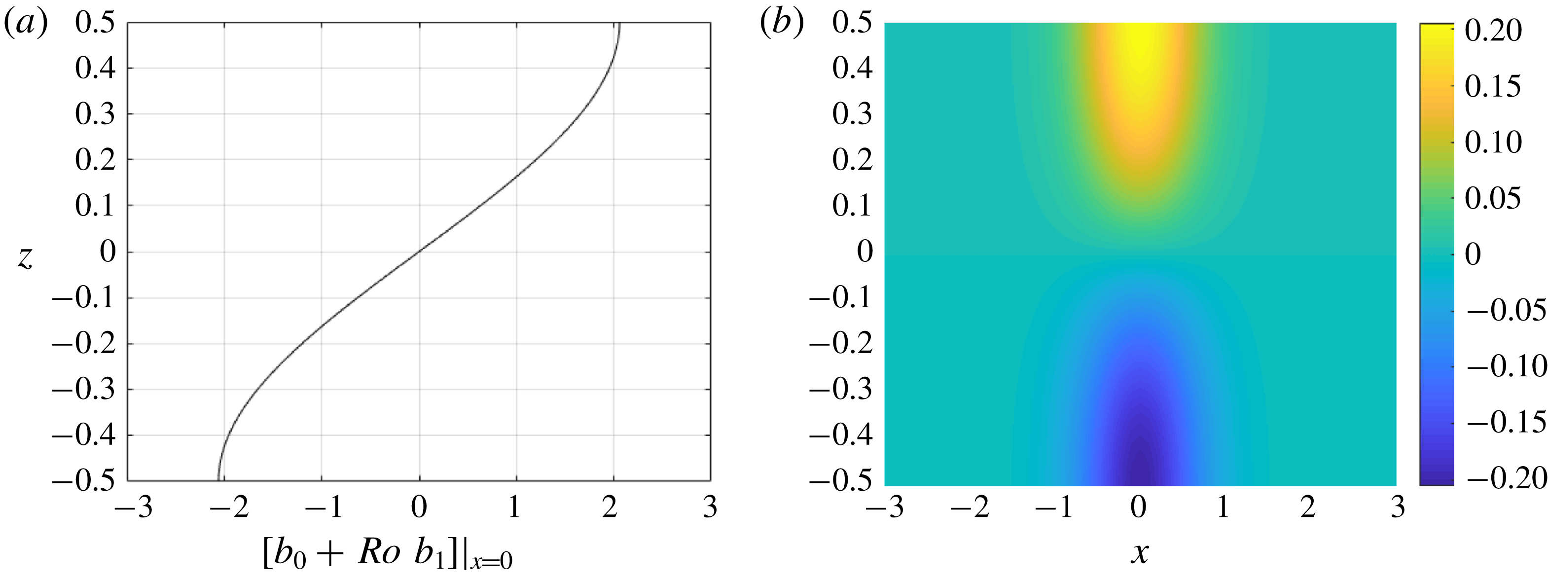
Figure 4 shows the
 $O(1)$
and
 $O(Ro)$
contributions to the buoyancy for
 $E=0.1$
,
 $Ro=0.01$
and
 $Pr=1$
and
 $b_{0}(x)=\tanh (x)$
. The
 $O(Ro)$
contribution to the buoyancy results in a slumping of the front towards a stable stratification.
(a) The steady-state buoyancy field to
 $O(Ro)$
at
 $x=0$
,
 $b(0,z)=b_{0}(0)+Ro\,b_{1}(0,z)$
; (b) the
 $O(Ro)$
correction term,
 $b_{1}(x,z)$
. Here,
 $E=0.1$
,
 $Ro=0.01$
,
 $Pr=1$
,
 $\unicode[STIX]{x1D708}=\unicode[STIX]{x1D705}=1$
and
 $b_{0}=\tanh (x)$
.
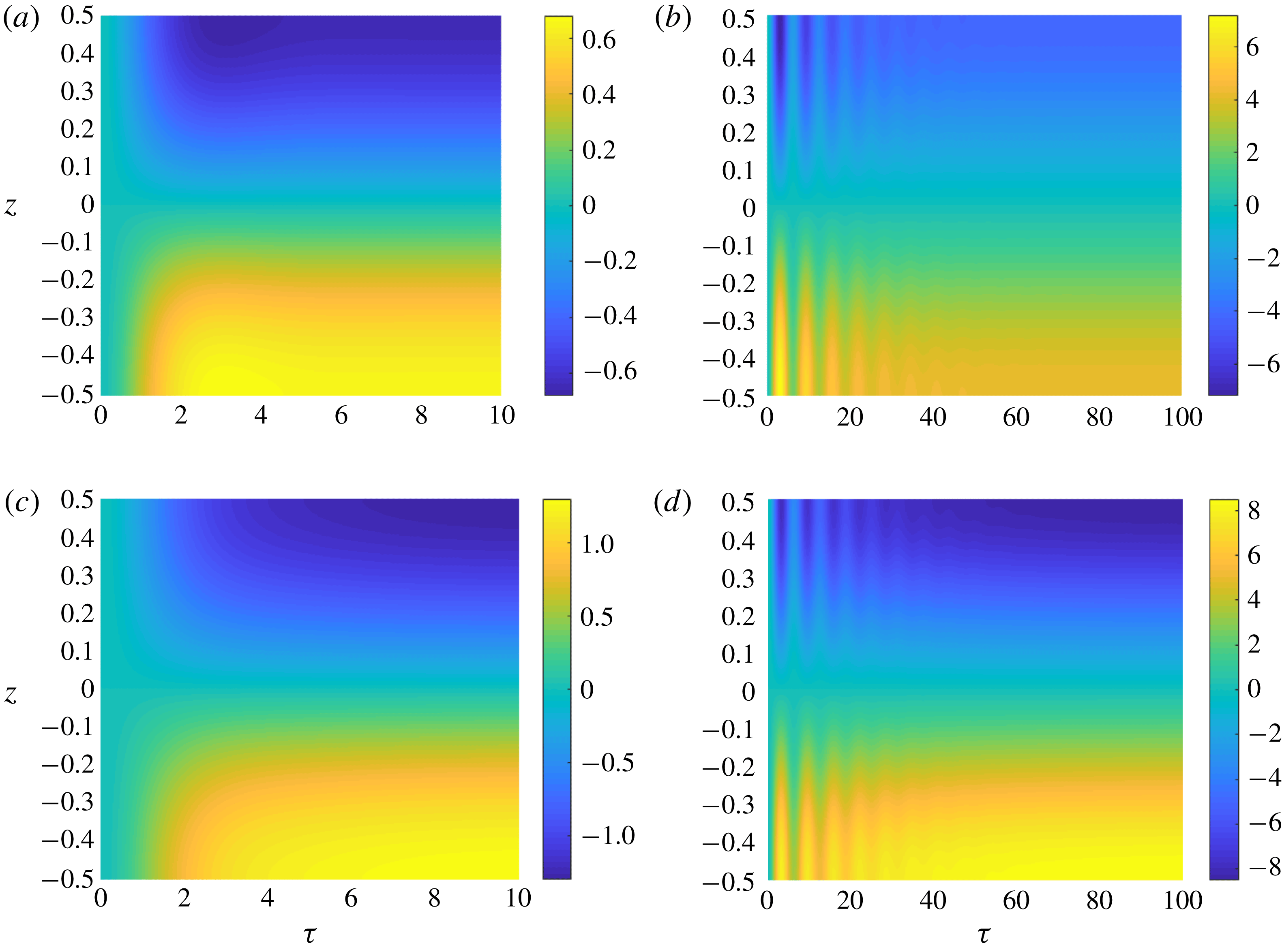
Plots of
 $M(z,\unicode[STIX]{x1D70F})$
for
 $(E,Pr)=(0.1,1)$
(a),
 $(0.01,1)$
(b),
 $(0.1,2)$
(c) and
 $(0.01,2)$
(d). We use
 $\unicode[STIX]{x1D708}=\unicode[STIX]{x1D705}=1$
and initial conditions
 $K(z,0)=0$
, corresponding to no initial flow, and
 $M(z,0)=0$
, corresponding to an initially depth-independent front. It should be noted that
 $b_{1}=-\sqrt{E}\,M|\unicode[STIX]{x1D735}_{H}b_{0}|^{2}$
.
As the front slumps, the surface buoyancy gradient can increase, corresponding to a sharpening of the front, hence allowing for short periods of frontogenesis. The horizontal buoyancy gradient is given by
 $$\begin{eqnarray}\unicode[STIX]{x1D735}_{H}b=\unicode[STIX]{x1D735}_{H}b_{0}(x,y,T)-\sqrt{E}\,Ro\,Pr\,K_{0}(z/\sqrt{E})\unicode[STIX]{x1D735}_{H}|\unicode[STIX]{x1D735}_{H}b_{0}|^{2}+O(Ro^{2}).\end{eqnarray}$$
At the upper surface where
 $K_{0}<0$
, the buoyancy gradient
 $(|\unicode[STIX]{x1D735}_{H}b|)$
is larger than its initial value
 $(|\unicode[STIX]{x1D735}_{H}b_{0}|)$
on the low-buoyancy side of the front, while the converse is true on the high-buoyancy side of the front. Along the midplane (
 $z=0$
),
 $K_{0}=0$
, and hence the buoyancy gradient is equal to
 $\unicode[STIX]{x1D735}_{H}b_{0}$
. It should be noted that the enhancement and reduction in the buoyancy gradient relative to
 $\unicode[STIX]{x1D735}_{H}b_{0}$
is
 $O(Ro)$
, and hence frontogenesis is a relatively weak effect for
 $Ro\ll 1$
.
Figure 5 shows the time-dependent
 $M(z,\unicode[STIX]{x1D70F})$
for four pairs of values of
 $(E,Pr)$
and initial conditions of no flow and no depth dependence in the buoyancy field. We can see that the system rapidly adjusts to a balanced state with inertial waves for small
 $E$
. Larger
 $Pr$
results in a longer adjustment period and more stable stratification.
3.3 The
$\boldsymbol{O}(\boldsymbol{R}\boldsymbol{o}^{2})$
buoyancy balance and shear dispersion

We now consider the
 $O(Ro^{2})$
buoyancy balance. The depth average of this balance allows us to determine the evolution of the leading-order buoyancy field,
 $b_{0}$
, over the slow time scale,
 $T$
. The evolution is found to be due to both shear dispersion and horizontal diffusion, although horizontal diffusion is only important at late times.
3.3.1 Depth-averaged buoyancy
The previous two sections examined the leading-order solutions to the time-dependent TTW equations. For initial conditions not in TTW balance, the leading-order contributions consist of an adjustment phase with damped inertial oscillations. The evolution of
 $\boldsymbol{u}_{0}$
and
 $b_{1}$
during the adjustment phase involves the fast time scale,
 $\unicode[STIX]{x1D70F}$
. After the end of the adjustment phase, the front will still evolve, but now on the slow time scale,
 $T$
. In this section, we examine the slow evolution of
 $b_{0}(x,z,T)$
by depth-averaging the
 $O(Ro^{2})$
buoyancy conservation equation.
The
 $O(Ro^{2})$
buoyancy equation is
 $$\begin{eqnarray}\frac{\unicode[STIX]{x2202}b_{0}}{\unicode[STIX]{x2202}T}+\frac{\unicode[STIX]{x2202}b_{2}}{\unicode[STIX]{x2202}\unicode[STIX]{x1D70F}}+\boldsymbol{u}_{1}\boldsymbol{\cdot }\unicode[STIX]{x1D735}_{H}b_{0}+\boldsymbol{u}_{0}\boldsymbol{\cdot }\unicode[STIX]{x1D735}b_{1}=\frac{E}{Pr}\frac{\unicode[STIX]{x2202}}{\unicode[STIX]{x2202}z}\left(\unicode[STIX]{x1D705}\frac{\unicode[STIX]{x2202}b_{2}}{\unicode[STIX]{x2202}z}\right)+\frac{\unicode[STIX]{x1D716}^{2}E}{Ro^{2}Pr}\unicode[STIX]{x1D705}\unicode[STIX]{x1D6FB}_{H}^{2}b_{0},\end{eqnarray}$$
where we note that
 $\unicode[STIX]{x1D716}=O(Ro)$
. We define the depth average as
 $$\begin{eqnarray}\overline{\ast }=\int _{-1/2}^{1/2}\ast \,\text{d}z\end{eqnarray}$$
and write a field
 $f$
as
 $f=\overline{f}+f^{\prime }$
, where
 $\overline{f^{\prime }}=0$
. We assume that the depth averages of the cross-front components of
 $\boldsymbol{u}_{H0},\boldsymbol{u}_{H1},\ldots$
and the depth averages of
 $b_{1},b_{2},\ldots \,$
are zero. This assumption holds if the initial conditions, the viscosity,
 $\unicode[STIX]{x1D708}$
, and the diffusivity,
 $\unicode[STIX]{x1D705}$
, are symmetric in
 $z$
about
 $z=0$
. We note that it is possible for depth-independent velocity components to develop, balanced by a depth-independent pressure term, but these lead to along-front velocities which do not affect buoyancy advection across the front and hence can be ignored. With this assumption, the depth-averaged buoyancy is simply
 $$\begin{eqnarray}\overline{b}=b_{0}(x,y,T).\end{eqnarray}$$
We now take a depth average of (3.44) and note that
 $\overline{\unicode[STIX]{x1D705}}=1$
to get
 $$\begin{eqnarray}\frac{\unicode[STIX]{x2202}b_{0}}{\unicode[STIX]{x2202}T}+\frac{\unicode[STIX]{x2202}}{\unicode[STIX]{x2202}x}\overline{u_{0}b_{1}}+\frac{\unicode[STIX]{x2202}}{\unicode[STIX]{x2202}y}\overline{v_{0}b_{1}}=\frac{\unicode[STIX]{x1D716}^{2}E}{Ro^{2}Pr}\unicode[STIX]{x1D6FB}_{H}^{2}b_{0},\end{eqnarray}$$
where
 $$\begin{eqnarray}\overline{\boldsymbol{u}_{H0}b_{1}}=(\overline{u_{0}b_{1}},\,\overline{v_{0}b_{1}})=E\,\overline{M\boldsymbol{K}}\boldsymbol{\cdot }\unicode[STIX]{x1D735}_{H}b_{0}|\unicode[STIX]{x1D735}_{H}b_{0}|^{2},\end{eqnarray}$$
so we can define a second-rank effective diffusivity tensor
 $\unicode[STIX]{x1D73F}_{eff}$
by
 $$\begin{eqnarray}-\overline{\boldsymbol{u}_{H0}b_{1}}=\unicode[STIX]{x1D73F}_{eff}\boldsymbol{\cdot }\unicode[STIX]{x1D735}_{H}b_{0},\end{eqnarray}$$
such that
 $$\begin{eqnarray}\unicode[STIX]{x1D73F}_{eff}=-E\,\overline{M\boldsymbol{K}}\,|\unicode[STIX]{x1D735}_{H}b_{0}|^{2},\end{eqnarray}$$
and allowing us to write (3.47) as
 $$\begin{eqnarray}\frac{\unicode[STIX]{x2202}b_{0}}{\unicode[STIX]{x2202}T}=\unicode[STIX]{x1D735}_{H}\boldsymbol{\cdot }\left[\unicode[STIX]{x1D73F}_{eff}\boldsymbol{\cdot }\unicode[STIX]{x1D735}_{H}b_{0}+\frac{\unicode[STIX]{x1D716}^{2}E}{Ro^{2}Pr}\unicode[STIX]{x1D735}_{H}b_{0}\right].\end{eqnarray}$$
Since
 $b_{0}$
does not evolve on the short time scale
 $\unicode[STIX]{x1D70F}$
, we can describe its evolution using the steady-state effective diffusivity,
 $\unicode[STIX]{x1D73F}_{eff}^{(0)}$
, given by
 $$\begin{eqnarray}\unicode[STIX]{x1D73F}_{eff}^{(0)}=-E\,\overline{M_{0}\boldsymbol{K}_{0}}\,|\unicode[STIX]{x1D735}_{H}b_{0}|^{2},\end{eqnarray}$$
where
 $M_{0}$
is given by (3.37) and
 $$\begin{eqnarray}\boldsymbol{K}_{0}=\left(\begin{array}{@{}cc@{}}E\displaystyle \frac{\unicode[STIX]{x2202}}{\unicode[STIX]{x2202}z}\left(\unicode[STIX]{x1D708}\displaystyle \frac{\unicode[STIX]{x2202}K_{0}}{\unicode[STIX]{x2202}z}\right) & -K_{0}\\ K_{0} & E\displaystyle \frac{\unicode[STIX]{x2202}}{\unicode[STIX]{x2202}z}\left(\unicode[STIX]{x1D708}\displaystyle \frac{\unicode[STIX]{x2202}K_{0}}{\unicode[STIX]{x2202}z}\right)\end{array}\right).\end{eqnarray}$$
We note that
 $$\begin{eqnarray}\int _{-1/2}^{1/2}E\frac{\unicode[STIX]{x2202}}{\unicode[STIX]{x2202}z}\left(\unicode[STIX]{x1D708}\frac{\unicode[STIX]{x2202}K_{0}}{\unicode[STIX]{x2202}z}\right)\left[\int _{-1/2}^{z}\frac{\unicode[STIX]{x1D708}}{\unicode[STIX]{x1D705}}\frac{\unicode[STIX]{x2202}K_{0}}{\unicode[STIX]{x2202}z^{\prime }}\,\text{d}z^{\prime }\right]\,\text{d}z=-\int _{-1/2}^{1/2}E\frac{\unicode[STIX]{x1D708}^{2}}{\unicode[STIX]{x1D705}}\left(\frac{\unicode[STIX]{x2202}K_{0}}{\unicode[STIX]{x2202}z}\right)^{2}\,\text{d}z<0;\end{eqnarray}$$
hence, the diagonal terms of
 $\overline{M_{0}\boldsymbol{K}_{0}}$
are negative, the diagonal terms of
 $\unicode[STIX]{x1D73F}_{eff}^{(0)}$
are positive and
 $\unicode[STIX]{x1D73F}_{eff}^{(0)}$
is positive definite.
Using
 $\unicode[STIX]{x1D73F}_{eff}^{(0)}$
, we write (3.51) as
 $$\begin{eqnarray}\frac{\unicode[STIX]{x2202}b_{0}}{\unicode[STIX]{x2202}T}=\unicode[STIX]{x1D735}_{H}\boldsymbol{\cdot }\left[-E\,\overline{M_{0}\boldsymbol{K}_{0}}\boldsymbol{\cdot }\unicode[STIX]{x1D735}_{H}b_{0}|\unicode[STIX]{x1D735}_{H}b_{0}|^{2}+\frac{\unicode[STIX]{x1D716}^{2}E}{Ro^{2}Pr}\unicode[STIX]{x1D735}_{H}b_{0}\right]\end{eqnarray}$$
and define
 $$\begin{eqnarray}\unicode[STIX]{x1D64C}(E)=-E\,\overline{M_{0}\boldsymbol{K}_{0}}/Pr\end{eqnarray}$$
for positive definite matrix
 $\unicode[STIX]{x1D64C}$
that depends only on
 $E$
. Hence, we can write the nonlinear diffusion equation, (3.55), as
 $$\begin{eqnarray}\frac{\unicode[STIX]{x2202}b_{0}}{\unicode[STIX]{x2202}T}=\unicode[STIX]{x1D735}_{H}\boldsymbol{\cdot }\left[Pr\unicode[STIX]{x1D64C}\boldsymbol{\cdot }\unicode[STIX]{x1D735}_{H}b_{0}|\unicode[STIX]{x1D735}_{H}b_{0}|^{2}+\frac{\unicode[STIX]{x1D716}^{2}E}{Ro^{2}Pr}\unicode[STIX]{x1D735}_{H}b_{0}\right].\end{eqnarray}$$
In the case of a
 $y$
-independent front,
 $b_{0}=b_{0}(x,T)$
, (3.57) reduces to
 $$\begin{eqnarray}\frac{\unicode[STIX]{x2202}b_{0}}{\unicode[STIX]{x2202}T}=\frac{\unicode[STIX]{x2202}}{\unicode[STIX]{x2202}x}\left[PrQ\left(\frac{\unicode[STIX]{x2202}b_{0}}{\unicode[STIX]{x2202}x}\right)^{3}+\frac{\unicode[STIX]{x1D716}^{2}E}{Ro^{2}Pr}\frac{\unicode[STIX]{x2202}b_{0}}{\unicode[STIX]{x2202}x}\right],\end{eqnarray}$$
where
 $$\begin{eqnarray}Q(E)=E^{2}\int _{-1/2}^{1/2}\frac{\unicode[STIX]{x1D708}^{2}}{\unicode[STIX]{x1D705}}\left(\frac{\unicode[STIX]{x2202}K_{0}}{\unicode[STIX]{x2202}z}\right)^{2}\,\text{d}z=E\int _{-1/2}^{1/2}\frac{\unicode[STIX]{x1D708}^{2}}{\unicode[STIX]{x1D705}}(K_{0}^{\prime })^{2}\,\text{d}z>0,\end{eqnarray}$$
since
 $K_{0}=K_{0}(z/\sqrt{E})$
and hence
 $\unicode[STIX]{x2202}K_{0}/\unicode[STIX]{x2202}z=E^{-1/2}K_{0}^{\prime }$
. Equation (3.58) is the Erdogan–Chatwin equation, first derived for longitudinal dispersion in pipe flow by Erdogan & Chatwin (Reference Erdogan and Chatwin1967). This equation arises in many non-rotating physical contexts where the dispersion rate is enhanced by buoyancy driven flow (Smith Reference Smith1982).
3.4 Shear dispersion in the limit of small Ekman number
Although the solution described in the previous sections is valid up to
 $E=O(1)$
, it is useful to examine the solution for small Ekman number, specifically
 $E=O(Ro)$
. In this limit, we recover a solution obtained previously by Garrett & Loder (Reference Garrett and Loder1981).
We can write the buoyancy frequency,
 $N^{2}$
, as
 $$\begin{eqnarray}N^{2}=\frac{\unicode[STIX]{x2202}b}{\unicode[STIX]{x2202}z}=Ro\frac{\unicode[STIX]{x2202}b_{1}}{\unicode[STIX]{x2202}z}+O(Ro^{2}),\end{eqnarray}$$
so
 $$\begin{eqnarray}N^{2}=-Ro\left(\sqrt{E}\frac{\unicode[STIX]{x2202}M}{\unicode[STIX]{x2202}z}\right)|\unicode[STIX]{x1D735}_{H}b_{0}|^{2}+O(Ro^{2}).\end{eqnarray}$$
During the spreading regime,
 $\sqrt{E}\,\unicode[STIX]{x2202}M/\unicode[STIX]{x2202}z=\sqrt{E}\,\unicode[STIX]{x2202}M_{0}/\unicode[STIX]{x2202}z=(Pr\,\unicode[STIX]{x1D708}/\unicode[STIX]{x1D705})K_{0}^{\prime }$
, so
 $$\begin{eqnarray}N^{2}=-Ro\,Pr\frac{\unicode[STIX]{x1D708}}{\unicode[STIX]{x1D705}}K_{0}^{\prime }(z/\sqrt{E})|\unicode[STIX]{x1D735}_{H}b_{0}|^{2}+O(Ro^{2}).\end{eqnarray}$$
In the case of
 $E=O(Ro)$
, the solution for velocity approaches that of thermal wind balance with
 $K_{0}(z/\sqrt{E})=-z/\sqrt{E}$
outside of thin Ekman layers near the top and bottom surfaces. These Ekman layers generate a depth-independent vertical velocity in the interior by Ekman pumping (Garrett & Loder Reference Garrett and Loder1981). The vertical velocity is independent of
 $z$
and the cross-front velocity is zero outside of the Ekman layers. Hence,
 $K_{0}^{\prime }\rightarrow -1$
, so
 $$\begin{eqnarray}N^{2}\sim Ro\,Pr\frac{\unicode[STIX]{x1D708}}{\unicode[STIX]{x1D705}}|\unicode[STIX]{x1D735}_{H}b_{0}|^{2}+O(Ro^{2}).\end{eqnarray}$$
In the 2d case, we have that
 $$\begin{eqnarray}\unicode[STIX]{x1D705}_{eff}=E\,Pr\left[\overline{\frac{\unicode[STIX]{x1D708}^{2}}{\unicode[STIX]{x1D705}}(K_{0}^{\prime })^{2}}\right]\left|\frac{\unicode[STIX]{x2202}b_{0}}{\unicode[STIX]{x2202}x}\right|^{2}.\end{eqnarray}$$
and from (3.62), to leading order,
 $$\begin{eqnarray}N^{2}=-Ro\,PrK_{0}^{\prime }\frac{\unicode[STIX]{x1D708}}{\unicode[STIX]{x1D705}}\,\left|\frac{\unicode[STIX]{x2202}b_{0}}{\unicode[STIX]{x2202}x}\right|^{2},\end{eqnarray}$$
and hence
 $$\begin{eqnarray}\unicode[STIX]{x1D705}_{eff}=\frac{E[\overline{\unicode[STIX]{x1D708}^{2}K_{0}^{\prime 2}/\unicode[STIX]{x1D705}}]N^{2}}{-Ro\,\unicode[STIX]{x1D708}\,K_{0}^{\prime }/\unicode[STIX]{x1D705}}.\end{eqnarray}$$
For small
 $E$
, we have
 $K_{0}^{\prime }\rightarrow -1$
, so
 $K_{0}^{\prime 2}\rightarrow 1$
. If we assume that
 $\unicode[STIX]{x1D708}$
and
 $\unicode[STIX]{x1D705}$
are approximately constant and equal in the interior region, away from the Ekman layers, the effective diffusivity is
 $$\begin{eqnarray}\unicode[STIX]{x1D705}_{eff}\sim \frac{N^{2}}{Ro}E,\end{eqnarray}$$
in the small-
 $E$
and -
 $Ro$
limit. We note that
 $N^{2}$
is approximately constant in the interior. Dimensionally, this result corresponds to
 $$\begin{eqnarray}\unicode[STIX]{x1D705}_{eff}\sim \frac{{\mathcal{N}}^{2}}{f^{2}}\overline{\unicode[STIX]{x1D708}}_{dim},\end{eqnarray}$$
where
 $\overline{\unicode[STIX]{x1D708}}_{dim}$
is the depth-averaged turbulent viscosity and
 ${\mathcal{N}}$
is the dimensional buoyancy frequency. This result was obtained previously by Garrett & Loder (Reference Garrett and Loder1981).
3.5 Self-similar solution
As the front spreads through shear dispersion on the slow time scale,
 $T$
, it adopts a self-similar cross-front profile. The self-similar solution can be obtained from the Erdogan–Chatwin equation (3.58). In this section, we will consider a two-dimensional front with
 $b_{0}=F(x,T)$
. This assumption is not necessary for the analysis but simplifies the notation. In this case, (3.58) can be written as
 $$\begin{eqnarray}\frac{\unicode[STIX]{x2202}F}{\unicode[STIX]{x2202}T}=\frac{\unicode[STIX]{x2202}}{\unicode[STIX]{x2202}x}\left[\left(c_{0}+c_{2}\left(\frac{\unicode[STIX]{x2202}F}{\unicode[STIX]{x2202}x}\right)^{2}\right)\frac{\unicode[STIX]{x2202}F}{\unicode[STIX]{x2202}x}\right],\end{eqnarray}$$
where
 $$\begin{eqnarray}c_{0}=\frac{\unicode[STIX]{x1D716}^{2}E}{Ro^{2}Pr}\quad \text{and}\quad c_{2}=PrQ(E),\end{eqnarray}$$
subject to boundary and initial conditions
 $$\begin{eqnarray}F\rightarrow \pm 1\quad \text{as }x\rightarrow \pm \infty \quad \text{and}\quad F(x,0)=f(x).\end{eqnarray}$$
We now consider the limit in which we can neglect horizontal diffusion, i.e.
 $c_{0}\simeq 0$
. This limit gives
 $$\begin{eqnarray}\frac{\unicode[STIX]{x2202}F}{\unicode[STIX]{x2202}T}=c_{2}\frac{\unicode[STIX]{x2202}}{\unicode[STIX]{x2202}x}\left(\frac{\unicode[STIX]{x2202}F}{\unicode[STIX]{x2202}x}\right)^{3}.\end{eqnarray}$$
We now seek a similarity solution of the form
 $$\begin{eqnarray}F(x,T)=F(\unicode[STIX]{x1D702})\quad \text{for similarity variable }\unicode[STIX]{x1D702}=\frac{x}{\unicode[STIX]{x1D6FE}T^{\unicode[STIX]{x1D6FC}}}.\end{eqnarray}$$
We note that it will not in general be possible to satisfy the initial condition
 $F(x,0)=f(x)$
; however, Smith (Reference Smith1982) showed that, in the case where the nonlinear diffusion dominates, the solutions to (3.69) will limit to this similarity solution for all nearby initial conditions. Using (3.72), we have
 $$\begin{eqnarray}-\frac{\unicode[STIX]{x1D6FC}\unicode[STIX]{x1D702}}{T}F^{\prime }=\frac{c_{2}}{\unicode[STIX]{x1D6FE}^{4}T^{4\unicode[STIX]{x1D6FC}}}(F^{\prime 3})^{\prime }.\end{eqnarray}$$
We let
 $\unicode[STIX]{x1D6FC}=1/4$
and
 $k_{2}=4c_{2}/\unicode[STIX]{x1D6FE}^{4}$
, so (3.74) becomes
 $$\begin{eqnarray}\unicode[STIX]{x1D702}F^{\prime }=-k_{2}(F^{\prime 3})^{\prime },\end{eqnarray}$$
which we can solve for
 $F^{\prime }$
; without loss of generality, we assume that
 $F^{\prime }(0)=1$
. The solution for
 $F^{\prime }$
is
 $$\begin{eqnarray}F^{\prime }(\unicode[STIX]{x1D702})=\left\{\begin{array}{@{}ll@{}}0,\quad & \unicode[STIX]{x1D702}<-\sqrt{3k_{2}},\\ \sqrt{1-{\displaystyle \frac{\unicode[STIX]{x1D702}^{2}}{3k_{2}}}},\quad & \unicode[STIX]{x1D702}\in \left[-\sqrt{3k_{2}},\sqrt{3k_{2}}\right],\\ 0,\quad & \unicode[STIX]{x1D702}>\sqrt{3k_{2}},\end{array}\right.\end{eqnarray}$$
which we integrate to obtain the solution (Smith Reference Smith1982)
 $$\begin{eqnarray}F(\unicode[STIX]{x1D702})=\left\{\begin{array}{@{}ll@{}}-1,\quad & \unicode[STIX]{x1D702}<-\sqrt{3k_{2}},\\ {\displaystyle \frac{1}{2}}\left[\unicode[STIX]{x1D702}\sqrt{1-{\displaystyle \frac{\unicode[STIX]{x1D702}^{2}}{3k_{2}}}}+\sqrt{3k_{2}}\arcsin \left({\displaystyle \frac{\unicode[STIX]{x1D702}}{\sqrt{3k_{2}}}}\right)\right],\quad & \unicode[STIX]{x1D702}\in \left[-\sqrt{3k_{2}},\sqrt{3k_{2}}\right],\\ 1,\quad & \unicode[STIX]{x1D702}>\sqrt{3k_{2}}.\end{array}\right.\end{eqnarray}$$
By matching
 $F(\pm \sqrt{3k_{2}})=\pm 1$
, we obtain
 $\sqrt{3k_{2}}=4/\unicode[STIX]{x03C0}$
; hence,
 $$\begin{eqnarray}k_{2}=\frac{16}{3\unicode[STIX]{x03C0}^{2}}\end{eqnarray}$$
and
 $$\begin{eqnarray}\unicode[STIX]{x1D6FE}=\left(\frac{3\unicode[STIX]{x03C0}^{2}c_{2}}{4}\right)^{1/4}.\end{eqnarray}$$
As
 $k_{2}$
is independent of
 $E$
and
 $Pr$
, we can see that the form of the solution is the same for all parameter ranges, with the parameters entering only through the spreading parameter
 $\unicode[STIX]{x1D6FE}$
which describes the frontal width.
We note that
 $F$
and
 $F^{\prime }$
are continuous while
 $F^{\prime \prime }$
diverges at the edge of the front, i.e. as
 $\unicode[STIX]{x1D702}\rightarrow \pm \sqrt{3k_{2}}$
, as
 $$\begin{eqnarray}F^{\prime \prime }(\unicode[STIX]{x1D702})=\left\{\begin{array}{@{}ll@{}}0,\quad & \unicode[STIX]{x1D702}<-\sqrt{3k_{2}},\\ -{\displaystyle \frac{\unicode[STIX]{x1D702}}{3k_{2}\sqrt{1-\unicode[STIX]{x1D702}^{2}/3k_{2}}}},\quad & \unicode[STIX]{x1D702}\in \left(-\sqrt{3k_{2}},\sqrt{3k_{2}}\right),\\ 0,\quad & \unicode[STIX]{x1D702}>\sqrt{3k_{2}}.\end{array}\right.\end{eqnarray}$$
When horizontal diffusion is included as in (3.69), this singularity is smoothed.
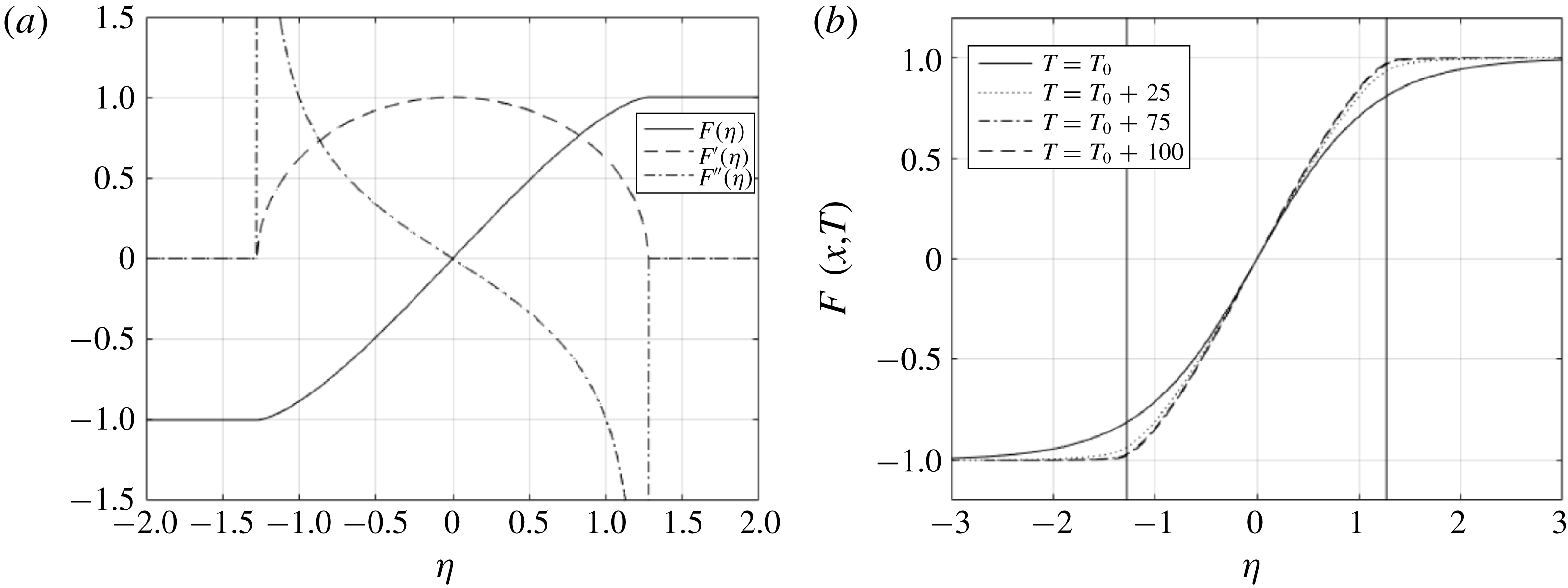
Figure 6(a) shows the similarity solution,
 $F(\unicode[STIX]{x1D702})$
, and its first and second derivatives. The function
 $F(\unicode[STIX]{x1D702})$
is approximately linear inside the front, with regions of large curvature at the edges. Figure 6(b) shows the numerical solution to (3.69) for
 $c_{0}=1.6\times 10^{-4}$
and
 $c_{2}=0.0208$
at
 $T=T_{0}$
,
 $T=T_{0}+25$
,
 $T=T_{0}+75$
and
 $T=T_{0}+100$
. The initial profile is given by
 $b(x,T_{0})=\tanh (x)$
for
 $T_{0}=4$
, and we see that this profile has evolved towards the similarity solution,
 $F(\unicode[STIX]{x1D702})$
, by time
 $T=T_{0}+75$
before spreading out in a self-similar manner for larger
 $T$
.
(a) Plots of the analytic similarity solution,
 $F(\unicode[STIX]{x1D702})$
, to (3.72) and derivatives
 $F^{\prime }(\unicode[STIX]{x1D702})$
and
 $F^{\prime \prime }(\unicode[STIX]{x1D702})$
. It should be noted that
 $b_{0}\propto F$
,
 $(u_{0},v_{0})\propto F^{\prime }$
and
 $w_{0}\propto F^{\prime \prime }$
. (b) The numerical solution to (3.69),
 $F(x,T)$
, with initial condition
 $b(x,T_{0})=\tanh (x)$
for
 $T_{0}=4$
,
 $E=0.1$
,
 $\unicode[STIX]{x1D708}=\unicode[STIX]{x1D705}=1$
,
 $Ro=0.05$
,
 $\unicode[STIX]{x1D716}=0.002$
and
 $Pr=1$
, corresponding to
 $c_{0}=1.6\times 10^{-4}$
and
 $c_{2}=0.0208$
. The initial condition in the numerical solution is imposed at
 $T=T_{0}$
to avoid the singularity in
 $\unicode[STIX]{x1D702}$
at
 $T=0$
. The vertical lines in (b) show the predicted frontal edges,
 $\unicode[STIX]{x1D702}=\pm 4/\unicode[STIX]{x03C0}$
.
By considering the relative magnitudes of the shear dispersion and horizontal diffusion terms, we find that our similarity solution is valid for
 $$\begin{eqnarray}t\ll \frac{Ro^{3}Pr^{3}Q(E)}{\unicode[STIX]{x1D716}^{4}E^{2}}.\end{eqnarray}$$
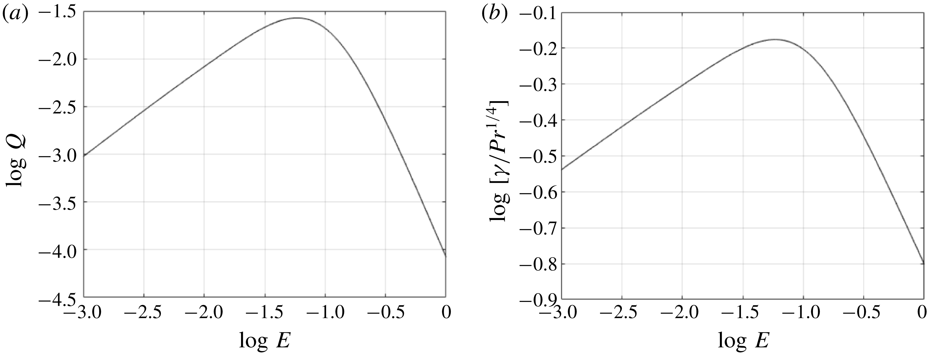
Figure 7 shows logarithmic plots of
 $Q$
and
 $\unicode[STIX]{x1D6FE}/Pr^{1/4}$
as functions of the Ekman number for constant
 $\unicode[STIX]{x1D708}$
. It should be noted from (3.69) and (3.70) that the effective diffusivity is proportional to
 $PrQ$
, while the frontal width is given by
 $$\begin{eqnarray}l_{f}(T)=8\unicode[STIX]{x1D6FE}T^{1/4}/\unicode[STIX]{x03C0},\end{eqnarray}$$
since the edges of the front correspond to
 $\unicode[STIX]{x1D702}=\pm \sqrt{3k_{2}}$
. As described in § 3.3.1, the effective diffusivity depends on the departure from the depth-averaged buoyancy,
 $b_{1}=-\sqrt{E}PrK_{0}|\unicode[STIX]{x2202}b_{0}/\unicode[STIX]{x2202}x|^{2}$
, and the cross-front velocity,
 $u_{0}=-\sqrt{E}K_{0}^{\prime \prime }\unicode[STIX]{x2202}b_{0}/\unicode[STIX]{x2202}x$
.
In the limit of small
 $E$
, the cross-front velocity becomes small as the system is approximately in thermal wind balance. As discussed in § 3.4, this leads to a small effective diffusivity, consistent with the result that
 $Q\sim E$
and
 $\unicode[STIX]{x1D6FE}\sim E^{1/4}$
in this limit (see figure 7). In the limit of large
 $E$
, strong vertical mixing causes the stratification and the cross-front velocity to decrease with increasing
 $E$
, resulting in a smaller effective diffusivity and slower spreading. In the limit of large
 $E$
,
 $Q\sim E^{-3}$
and
 $\unicode[STIX]{x1D6FE}\sim E^{-3/4}$
, consistent with this description. The effective diffusivity and spreading rate are maximum for an intermediate value of
 $E\approx 0.06$
. See appendix A for a more complete description of the dependence of
 $u_{0}$
and
 $b_{1}$
on
 $E$
.
Logarithmic plots of
 $Q(E)$
(a) and
 $\unicode[STIX]{x1D6FE}/Pr^{1/4}$
(b) as functions of
 $E$
for constant
 $\unicode[STIX]{x1D708}$
. It should be noted that
 $\unicode[STIX]{x1D6FE}/Pr^{1/4}$
depends only on
 $E$
and the frontal width is proportional to
 $\unicode[STIX]{x1D6FE}T^{1/4}$
.
Ferrari & Young (Reference Ferrari and Young1997) consider a frontal problem using an ‘intermittent mixing’ parametrisation where the tracers are advected freely until time
 $t=t_{mix}$
where the vertical tracer profile is instantaneously set to its vertical average and the process is repeated. The governing equation for the depth-independent buoyancy profile is of the same form as (3.72) with a different value of
 $c_{2}$
; hence, it admits the same similarity solution. This will be true for any parametrised model in which the leading-order velocity is linear in the buoyancy gradient,
 $u\approx c(z)\overline{b}_{x}$
, and the leading-order buoyancy flux scales as
 $F_{b}=\overline{ub}\sim \overline{uD_{z}u}\,\overline{b}_{x}\sim \overline{b}_{x}^{3}$
for some linear
 $z$
-dependent operator
 $D_{z}$
, which is determined by the parametrisation. We note that the vertical profiles of velocity and buoyancy differ between models, although the leading-order depth-averaged tracer profiles have the same form over long times.
Plots of
 $b_{0}(x,T)$
(a),
 $N_{0}^{2}(x,z,T)=Ro\,\unicode[STIX]{x2202}b_{1}/\unicode[STIX]{x2202}z$
at
 $z=0$
(b),
 $M_{0}^{2}(x,T)=\unicode[STIX]{x2202}b_{0}/\unicode[STIX]{x2202}x$
(c) and
 $u_{0}(x,z,T)$
at
 $z=1/2$
(d) for
 $E=0.1$
,
 $Ro=0.01$
and
 $Pr=1$
. We use the similarity solution for
 $b_{0}$
and assume that all transients have decayed. It should be noted that
 $b_{0}\sim F$
,
 $N_{0}^{2}\sim F^{\prime 2}$
and
 $M_{0}^{2},u_{0}\sim F^{\prime }$
.

Figure 8 shows the long-term evolution of the background buoyancy, buoyancy gradients and cross-front velocity using the similarity solution. We can see that as the front spreads, both the vertical and the horizontal buoyancy gradients decrease and the cross-front velocity decelerates. Since the vertical buoyancy stratification formed by the initial slumping is maintained by the cross-front velocity shear, this stratification weakens as expected when the cross-front velocity decelerates. The along-front velocity,
 $v_{0}$
, and vertical velocity,
 $w_{0}$
, also decrease as the front spreads.
It should be noted that the vertical structure of the buoyancy perturbation,
 $b_{1}$
, and the velocities,
 $(u_{0},v_{0},w_{0})$
, are independent of the long time scale,
 $T$
, and assuming that any transients have decayed, only depend on the depth
 $z$
and Ekman number.
3.6 Summary of the analytic solution
Combining our results from the
 $O(1)$
,
 $O(Ro)$
and
 $O(Ro^{2})$
balances, we can write our analytic solution as
 $$\begin{eqnarray}\displaystyle \boldsymbol{u}_{H}(x,y,z,\unicode[STIX]{x1D70F},T) & = & \displaystyle -\sqrt{E}\,\boldsymbol{K}(z,\unicode[STIX]{x1D70F})\boldsymbol{\cdot }\unicode[STIX]{x1D735}_{H}b_{0}(x,y,T)+O(Ro),\end{eqnarray}$$
 $$\begin{eqnarray}\displaystyle w(x,y,z,\unicode[STIX]{x1D70F},T) & = & \displaystyle E\left[\int _{-1/2}^{z}\frac{-L_{\unicode[STIX]{x1D708}}K(z^{\prime },\unicode[STIX]{x1D70F})}{\sqrt{E}}\,\text{d}z^{\prime }\right]\unicode[STIX]{x1D6FB}_{H}^{2}b_{0}(x,y,T)+O(Ro),\end{eqnarray}$$
 $$\begin{eqnarray}\displaystyle b(x,y,z,\unicode[STIX]{x1D70F},T) & = & \displaystyle b_{0}(x,y,T)-Ro\,\sqrt{E}\,M(z,\unicode[STIX]{x1D70F})|\unicode[STIX]{x1D735}_{H}b_{0}(x,y,T)|^{2}+O(Ro^{2}),\qquad\end{eqnarray}$$
 $b_{0}$
satisfies
 $$\begin{eqnarray}\frac{\unicode[STIX]{x2202}b_{0}}{\unicode[STIX]{x2202}T}=\unicode[STIX]{x1D735}_{H}\boldsymbol{\cdot }\left[Pr\unicode[STIX]{x1D64C}\boldsymbol{\cdot }\unicode[STIX]{x1D735}_{H}b_{0}|\unicode[STIX]{x1D735}_{H}b_{0}|^{2}+\frac{\unicode[STIX]{x1D716}^{2}E}{Ro^{2}Pr}\unicode[STIX]{x1D735}_{H}b_{0}\right].\end{eqnarray}$$
4 Conclusions and discussion
Here, we have examined the influence of small-scale turbulence on the adjustment and spreading of density fronts in a rotating reference frame using a multiple-time-scale analysis and asymptotic analysis. After a short initial adjustment period, a self-similar spreading regime develops in which an effective horizontal diffusion results from the coupling of a vertically sheared cross-front flow and vertical diffusion. During the initial adjustment period, weak frontogenesis is possible due to the slumping of the front while the long-term spreading is always frontolytic.
The time dependence and similarity solutions during the spreading phase have been calculated analytically using an expansion in small Rossby number, and allow us to predict the rate of spreading for a wide range of Ekman and Rossby numbers. The dominant balance in the buoyancy equation is between vertical diffusion and cross-front advection, resulting in a buoyancy field consisting of both spreading and slumping components in a dynamic equilibrium. The dominant balance in the momentum equations is the TTW balance between Coriolis forces, vertical momentum mixing and horizontal pressure gradients, for which analytic and numerical solutions have been presented. This balance holds until the effects of horizontal diffusion become significant at late times.
Horizontal spreading of the depth-averaged buoyancy results from shear dispersion, which dominates the horizontal turbulent diffusion in the frontal region until late times (3.81). The spreading is described by the nonlinear Erdogan–Chatwin (Erdogan & Chatwin Reference Erdogan and Chatwin1967) equation, which arises in many contexts and has solutions that tend to a similarity solution in the region where shear dispersion dominates. Shear dispersion leads to a cross-front density profile that is nearly linear inside the front, with high curvature at the edges of the frontal zone. High curvature is associated with large vertical velocity through the TTW balance, which results in up-/downwelling confined to thin bands at the edges of the front. Qualitatively, this result is similar to the velocity confinement effect observed by Shakespeare & Taylor (Reference Shakespeare and Taylor2013) for inviscid strain-driven fronts, although it arises from a different mechanism.
Dimensionally, we can write the frontal width as
 $$\begin{eqnarray}L_{f}(t)=\left(\frac{3072}{\unicode[STIX]{x03C0}^{2}}\right)^{1/4}\left[\frac{Q(E)H^{2}\unicode[STIX]{x0394}b^{2}Pr}{f^{3}}\right]^{1/4}t^{1/4}\end{eqnarray}$$
using (3.82), and hence the spreading rate is given by
 $$\begin{eqnarray}\frac{\text{d}L_{f}}{\text{d}t}=\frac{768}{\unicode[STIX]{x03C0}^{2}}\left[\frac{Q(E)H^{2}\unicode[STIX]{x0394}b^{2}Pr}{f^{3}}\right]L_{f}^{-3},\end{eqnarray}$$
where
 $Q(E)$
is defined in (3.59). For a typical ocean front with
 $H\sim 100~\text{m}$
,
 $L_{f}\sim 10~\text{km}$
,
 $f\sim 10^{-4}~\text{s}^{-1}$
and
 $\unicode[STIX]{x0394}\unicode[STIX]{x1D70C}\sim 0.1~\text{kg}~\text{m}^{-3}$
, the observed frontal spreading would occur at a rate of order 1 km per day for an Ekman number of
 $E=0.1$
(corresponding to a turbulent viscosity of
 $\unicode[STIX]{x1D708}\sim 0.1~\text{m}^{2}~\text{s}^{-1}$
). By comparison, spreading due to horizontal diffusion would just be of the order of 1 m per day for the same parameters.
Using scaling arguments, we can relate the Ekman number to the turbulent viscosity associated with convection driven by a surface heat flux,
 $J_{0}$
, or a surface wind stress,
 $\unicode[STIX]{x1D70F}_{w}$
. In the case of convection, the turbulent Ekman number scales according to (Taylor & Ferrari Reference Taylor and Ferrari2011)
 $$\begin{eqnarray}E\simeq \frac{C}{f}\left(\frac{J_{0}\unicode[STIX]{x1D6FC}g}{c_{p}\unicode[STIX]{x1D70C}_{0}H^{2}}\right)^{1/3},\end{eqnarray}$$
where
 $H$
is the depth of the convective layer,
 $\unicode[STIX]{x1D70C}_{0}$
is the water density,
 $c_{p}$
is the heat capacity,
 $\unicode[STIX]{x1D6FC}$
is the thermal expansion coefficient,
 $C$
is an empirical scaling constant and
 $g$
is gravitational acceleration. Using typical values for the ocean, including a convective layer depth of 100 m and
 $f=10^{-4}~\text{s}^{-1}$
, typical heat flux values in the range
 $Q_{0}=1{-}1000~\text{W}~\text{m}^{-2}$
correspond to Ekman numbers in the range
 $E\simeq 0.1{-}1$
. Similarly, the Ekman number can be related to the wind stress using (Enriquez & Taylor Reference Enriquez and Taylor2015)
 $$\begin{eqnarray}E\simeq \frac{C}{fH}\left(\frac{\unicode[STIX]{x1D70F}_{w}}{\unicode[STIX]{x1D70C}_{0}}\right)^{1/2},\end{eqnarray}$$
and a wind stress of
 $\unicode[STIX]{x1D70F}_{w}=1~\text{N}~\text{m}^{-2}$
corresponds to
 $E\simeq 0.1$
.
In our analysis, the only mechanism driving frontogenesis is the coupling between the cross-front velocity and the along-front thermal wind through the turbulent mixing. For less idealised flows, the tendency for fronts to sharpen or spread is governed by a competition between the classical frontogenesis function and the effects of turbulent mixing. Interestingly, we observe that turbulent mixing can both sharpen and spread fronts, with sharpening associated with frontogenesis during an initial adjustment phase and spreading associated with shear dispersion.
In the ocean and atmosphere, deformation of fronts by larger-scale circulation can generate cross-front circulation that can drive further frontogenesis (Hoskins & Bretherton Reference Hoskins and Bretherton1972). Shear dispersion through vertical mixing might provide a mechanism to arrest deformation-driven frontogenesis, which can lead to finite-time singularities (Hoskins & Bretherton Reference Hoskins and Bretherton1972). Future work could include externally imposed large-scale strain to examine frontal arrest, which would provide insight into the properties of equilibrated fronts.
To simplify our analysis, we have kept the viscosity and diffusivity independent of time. Recent observations and numerical simulations have found that turbulence can be significantly enhanced at strong fronts, including the Kuroshio (D’Asaro et al. Reference D’Asaro, Lee, Rainville, Harcourt and Thomas2011), the Gulf Stream (Thomas et al. Reference Thomas, Taylor, Ferrari and Joyce2013) and the California Current (Johnston, Rudnick & Pallàs-Sanz Reference Johnston, Rudnick and Pallàs-Sanz2011). On the other hand, the stable stratification that develops as a front slumps has been implicated in the suppression of turbulent mixing (Taylor & Ferrari Reference Taylor and Ferrari2010; Taylor Reference Taylor2016). It remains unclear how small-scale turbulence depends on the large-scale properties of the front and the surface wind and buoyancy forcing. In either case, the turbulent viscosity and diffusivity probably vary with position across the front and in time, effects that are neglected here. Varying levels of small-scale turbulence could lead to a feedback between the evolution of the front through TTW balance and turbulent mixing. The coupled response of turbulence and frontal dynamics will be the topic of future work.
Acknowledgements
The authors would like to thank R. Ferrari, J. McWilliams, L. Thomas and J. Wenegrat for stimulating and helpful conversations. We are also very grateful to B. Young for comments on an early draft of the paper and for pointing out various connections with previous literature on shear dispersion.
Appendix A. Analytic solution for the
$O(1)$
velocity for constant
$\unicode[STIX]{x1D742}$


We assume constant viscosity,
 $\unicode[STIX]{x1D708}=1$
, to find an analytic solution for the structure function
 $K_{0}$
. Equation (3.15) becomes
 $$\begin{eqnarray}-K_{0}^{(4)}=K_{0}+\unicode[STIX]{x1D701},\end{eqnarray}$$
with boundary conditions
 $K_{0}^{\prime }=K_{0}^{\prime \prime \prime }=0$
at
 $\unicode[STIX]{x1D701}=\pm \unicode[STIX]{x1D701}_{0}$
, where
 $\unicode[STIX]{x1D701}_{0}=1/\sqrt{4E}$
. This is a fourth-order ordinary differential equation which can be solved analytically. The exponents of the independent solutions are
 $(1\pm \text{i})/\sqrt{2}$
and
 $(-1\pm \text{i})/\sqrt{2}$
, so, since the system is clearly odd in
 $\unicode[STIX]{x1D701}$
, we use symmetry to obtain the solution
 $$\begin{eqnarray}K_{0}=-\unicode[STIX]{x1D701}+C_{+}\text{cs}(\unicode[STIX]{x1D701})+C_{-}\text{sc}(\unicode[STIX]{x1D701}),\end{eqnarray}$$
where
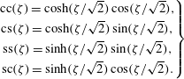 $$\begin{eqnarray}\left.\begin{array}{@{}c@{}}\text{cc}(\unicode[STIX]{x1D701})=\cosh (\unicode[STIX]{x1D701}/\sqrt{2})\cos (\unicode[STIX]{x1D701}/\sqrt{2}),\\ \text{cs}(\unicode[STIX]{x1D701})=\cosh (\unicode[STIX]{x1D701}/\sqrt{2})\sin (\unicode[STIX]{x1D701}/\sqrt{2}),\\ \text{ss}(\unicode[STIX]{x1D701})=\sinh (\unicode[STIX]{x1D701}/\sqrt{2})\sin (\unicode[STIX]{x1D701}/\sqrt{2}),\\ \text{sc}(\unicode[STIX]{x1D701})=\sinh (\unicode[STIX]{x1D701}/\sqrt{2})\cos (\unicode[STIX]{x1D701}/\sqrt{2}).\end{array}\right\}\end{eqnarray}$$
From the boundary conditions,
 $K_{0}^{\prime }(\unicode[STIX]{x1D701}_{0})=K_{0}^{\prime \prime \prime }(\unicode[STIX]{x1D701}_{0})=0$
, we get
 $$\begin{eqnarray}\left(\begin{array}{@{}cc@{}}\text{cc}(\unicode[STIX]{x1D701}_{0})+\text{ss}(\unicode[STIX]{x1D701}_{0}) & \text{cc}(\unicode[STIX]{x1D701}_{0})-\text{ss}(\unicode[STIX]{x1D701}_{0})\\ \text{cc}(\unicode[STIX]{x1D701}_{0})-\text{ss}(\unicode[STIX]{x1D701}_{0}) & -\text{cc}(\unicode[STIX]{x1D701}_{0})-\text{ss}(\unicode[STIX]{x1D701}_{0})\end{array}\right)\left(\begin{array}{@{}c@{}}C_{+}\\ C_{-}\end{array}\right)=\left(\begin{array}{@{}c@{}}\sqrt{2}\\ 0\end{array}\right),\end{eqnarray}$$
which we invert to get
 $$\begin{eqnarray}C_{\pm }=\frac{1}{\sqrt{2}}\frac{\text{cc}(\unicode[STIX]{x1D701}_{0})\pm \text{ss}(\unicode[STIX]{x1D701}_{0})}{\text{cc}^{2}(\unicode[STIX]{x1D701}_{0})+\text{ss}^{2}(\unicode[STIX]{x1D701}_{0})}.\end{eqnarray}$$
We can also solve for
 ${\mathcal{Z}}_{n}$
analytically using (3.21), which reduces to
 $$\begin{eqnarray}\frac{\unicode[STIX]{x2202}^{2}{\mathcal{Z}}_{n}}{\unicode[STIX]{x2202}z^{2}}=-\unicode[STIX]{x1D706}_{n}{\mathcal{Z}}_{n}.\end{eqnarray}$$
We obtain solutions
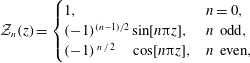 $$\begin{eqnarray}{\mathcal{Z}}_{n}(z)=\left\{\begin{array}{@{}ll@{}}1,\quad & n=0,\\ (-1)^{(n-1)/2}\sin [n\unicode[STIX]{x03C0}z],\quad & n\text{ odd},\\ (-1)^{\,\,n\,/\,2}\quad \cos [n\unicode[STIX]{x03C0}z],\quad & n\text{ even},\end{array}\right.\end{eqnarray}$$
for
 $$\begin{eqnarray}\unicode[STIX]{x1D706}_{n}=n^{2}\unicode[STIX]{x03C0}^{2},\end{eqnarray}$$
and
 $$\begin{eqnarray}z_{n}^{2}=\left\{\begin{array}{@{}ll@{}}1,\quad & n=0,\\ {\textstyle \frac{1}{2}},\quad & n\in \mathbb{N},\end{array}\right.\end{eqnarray}$$
and integrate to get
 $$\begin{eqnarray}\int _{-1/2}^{z}{\mathcal{Z}}_{n}(z^{\prime })\,\text{d}z^{\prime }=\left\{\begin{array}{@{}ll@{}}z+{\textstyle \frac{1}{2}},\quad & n=0,\\ (-1)^{(n+1)/2}{\displaystyle \frac{\cos [(1+2n)\unicode[STIX]{x03C0}z]}{n\unicode[STIX]{x03C0}}},\quad & n\text{ odd},\\ (-1)^{n/2}{\displaystyle \frac{\sin [(1+2n)\unicode[STIX]{x03C0}z]}{n\unicode[STIX]{x03C0}}},\quad & n\text{ even}.\end{array}\right.\end{eqnarray}$$
We plot
 $K_{0}$
and
 ${\mathcal{Z}}_{n}$
in appendix C when considering the numerical solutions for general
 $\unicode[STIX]{x1D708}$
; see figures 11 and 12(a,b).
We now consider the Ekman number dependence of
 $K_{0}$
in the case of constant
 $\unicode[STIX]{x1D708}$
and
 $\unicode[STIX]{x1D705}$
, and
 $Pr=1$
. We find that there are regimes for small and large
 $E$
where the maximum values of
 $K_{0}$
and its derivatives obey power law dependences on
 $E$
. These are given in table 2 and can be calculated by expanding (A 2) for small and large
 $E$
.
The Ekman number dependence of the maximum values of
 $K_{0}(\unicode[STIX]{x1D701})$
,
 $K_{0}^{\prime }(\unicode[STIX]{x1D701})$
,
 $K_{0}^{\prime \prime }(\unicode[STIX]{x1D701})$
,
 $\sqrt{E}K_{0}(\unicode[STIX]{x1D701})$
,
 $EK_{0}^{\prime }(\unicode[STIX]{x1D701})$
and
 $\sqrt{E}K_{0}^{\prime \prime }(\unicode[STIX]{x1D701})$
for
 $\unicode[STIX]{x1D701}=z/\sqrt{E}$
in the case of small and large
 $E$
. Here, we ignore any constant coefficients.

The maximum values for
 $K_{0}$
and
 $K_{0}^{\prime \prime }$
occur at the boundaries, as the horizontal velocity is highest at the surface while the maximum for
 $K_{0}^{\prime }$
occurs in the interior of the vertical domain corresponding to the location of the maximum vertical velocity.
Logarithmic plots of the maximum magnitude as a function of the Ekman number of (a)
 $K_{0}(\unicode[STIX]{x1D701})$
,
 $K_{0}^{\prime }(\unicode[STIX]{x1D701})$
and
 $K_{0}^{\prime \prime }(\unicode[STIX]{x1D701})$
and (b)
 $\sqrt{E}K_{0}(\unicode[STIX]{x1D701})$
,
 $EK_{0}^{\prime }(\unicode[STIX]{x1D701})$
and
 $\sqrt{E}K_{0}^{\prime \prime }(\unicode[STIX]{x1D701})$
for
 $\unicode[STIX]{x1D701}=z/\sqrt{E}$
.
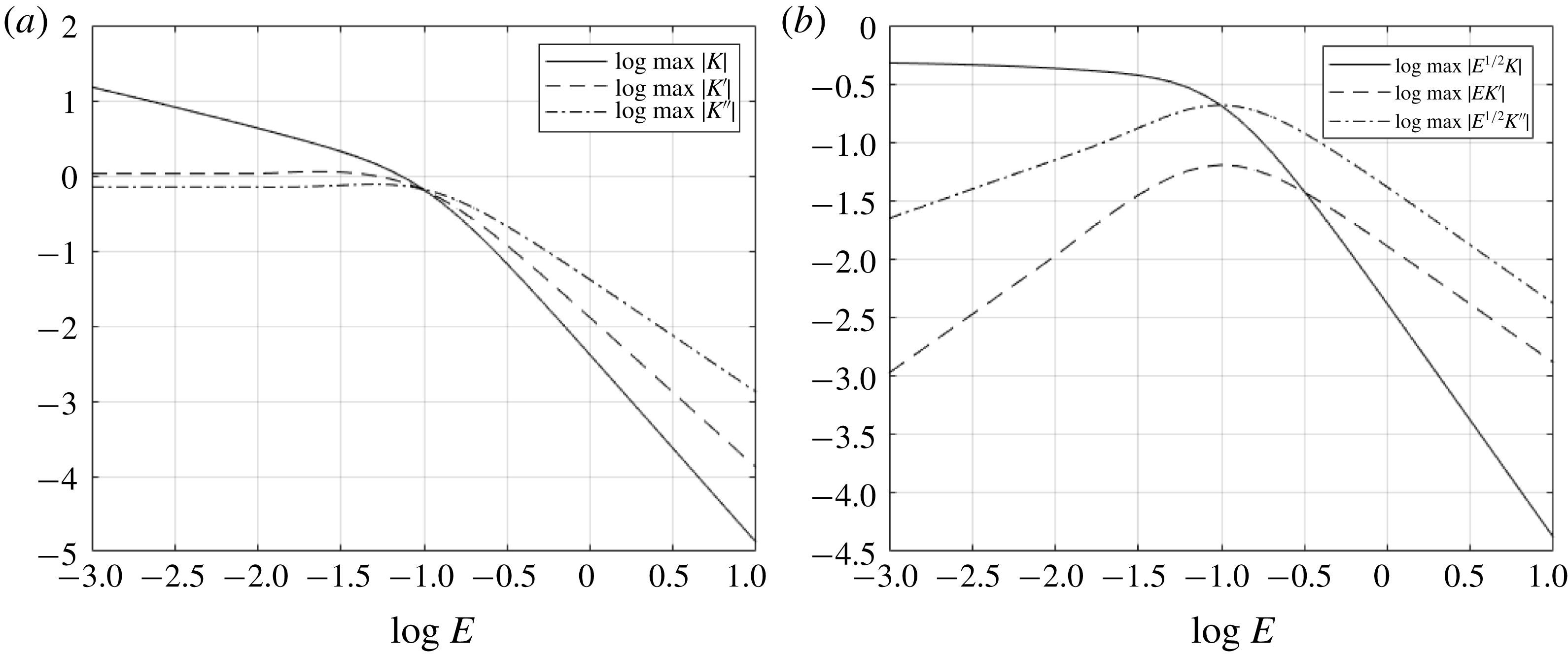
Figure 9 shows logarithmic plots of the maximum magnitude of
 $K_{0}(\unicode[STIX]{x1D701})$
,
 $K_{0}^{\prime }(\unicode[STIX]{x1D701})$
,
 $K_{0}^{\prime \prime }(\unicode[STIX]{x1D701})$
,
 $\sqrt{E}K_{0}(\unicode[STIX]{x1D701})$
,
 $EK_{0}^{\prime }(\unicode[STIX]{x1D701})$
and
 $\sqrt{E}K_{0}^{\prime \prime }(\unicode[STIX]{x1D701})$
as functions of the Ekman number. We can see that for small
 $E$
, the along-front velocity, proportional to
 $\sqrt{E}\,K_{0}$
, approaches a constant value corresponding to the surface velocity from the thermal wind balance profile. The cross-front and vertical velocities tend to zero for small
 $E$
, in agreement with thermal wind balance. For large
 $E$
, all velocity components become small as motion is damped by the high viscosity. We note that there is a maximum for both the vertical and the cross-front velocities at
 $E\approx 0.1$
. Analytically, we can show that
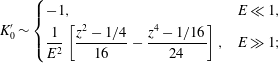 $$\begin{eqnarray}K_{0}^{\prime }\sim \left\{\begin{array}{@{}ll@{}}-1,\quad & E\ll 1,\\ {\displaystyle \frac{1}{E^{2}}}\left[{\displaystyle \frac{z^{2}-1/4}{16}}-{\displaystyle \frac{z^{4}-1/16}{24}}\right],\quad & E\gg 1;\end{array}\right.\end{eqnarray}$$
hence,
 $$\begin{eqnarray}Q(E)\sim \left\{\begin{array}{@{}ll@{}}E,\quad & E\ll 1,\\ {\textstyle \frac{31}{362\,880}}E^{-3},\quad & E\gg 1,\end{array}\right.\end{eqnarray}$$
in agreement with figure 7.
Appendix B. Solution for
$M$
with arbitrary
$\unicode[STIX]{x1D742}$
and
$\unicode[STIX]{x1D73F}$


To solve for
 $M$
with arbitrary
 $\unicode[STIX]{x1D708}$
and
 $\unicode[STIX]{x1D705}$
, we take the Laplace transform of (3.36) to get
 $$\begin{eqnarray}\left[s-\frac{E}{Pr}\frac{\unicode[STIX]{x2202}}{\unicode[STIX]{x2202}z}\left(\unicode[STIX]{x1D705}\frac{\unicode[STIX]{x2202}}{\unicode[STIX]{x2202}z}\right)\right]\widetilde{M}(z,s)-M(z,0)=\widetilde{P}(z,s),\end{eqnarray}$$
where we take
 $M(z,0)={\mathcal{M}}(z)$
as our initial state. We usually take
 ${\mathcal{M}}=0$
, corresponding to a depth-independent front; if we were instead to consider a balanced initial set-up, the solution would be given by the steady-state solution,
 $M_{0}$
. The forcing term,
 $\widetilde{P}$
, is given by
 $$\begin{eqnarray}\widetilde{P}(z,s)=\left[s-E\frac{\unicode[STIX]{x2202}}{\unicode[STIX]{x2202}z}\left(\unicode[STIX]{x1D708}\frac{\unicode[STIX]{x2202}}{\unicode[STIX]{x2202}z}\right)\right]\widetilde{K}(z,s)-{\mathcal{K}}(z),\end{eqnarray}$$
where we can use (3.25) to write
 $$\begin{eqnarray}\widetilde{K}(z,s)=\frac{1}{s}K_{0}(z/\sqrt{E})+\mathop{\sum }_{n=0}^{\infty }B_{n}\left[\frac{s+2E\unicode[STIX]{x1D706}_{n}}{(s+E\unicode[STIX]{x1D706}_{n})^{2}+1}\right]{\mathcal{Z}}_{n}(z),\end{eqnarray}$$
so
 $$\begin{eqnarray}\widetilde{P}(z,s)=[K_{0}-{\mathcal{K}}]-\frac{1}{s}E\frac{\unicode[STIX]{x2202}}{\unicode[STIX]{x2202}z}\left(\unicode[STIX]{x1D708}\frac{\unicode[STIX]{x2202}K_{0}}{\unicode[STIX]{x2202}z}\right)+\mathop{\sum }_{n=0}^{\infty }B_{n}\left[\frac{(s+E\unicode[STIX]{x1D706}_{n})(s+2E\unicode[STIX]{x1D706}_{n})}{(s+E\unicode[STIX]{x1D706}_{n})^{2}+1}\right]{\mathcal{Z}}_{n}(z).\end{eqnarray}$$
We note that
 $$\begin{eqnarray}K_{0}-{\mathcal{K}}=-\mathop{\sum }_{n=0}^{\infty }B_{n}{\mathcal{Z}}_{n}(z);\end{eqnarray}$$
hence,
 $$\begin{eqnarray}\widetilde{P}(z,s)=-\frac{1}{s}E\frac{\unicode[STIX]{x2202}}{\unicode[STIX]{x2202}z}\left(\unicode[STIX]{x1D708}\frac{\unicode[STIX]{x2202}K_{0}}{\unicode[STIX]{x2202}z}\right)+\mathop{\sum }_{n=0}^{\infty }B_{n}\left[\frac{E\unicode[STIX]{x1D706}_{n}(s+E\unicode[STIX]{x1D706}_{n})-1}{(s+E\unicode[STIX]{x1D706}_{n})^{2}+1}\right]{\mathcal{Z}}_{n}(z).\end{eqnarray}$$
We now write
 $$\begin{eqnarray}\widetilde{M}=\mathop{\sum }_{n=0}^{\infty }\widetilde{C}_{n}(s){\mathcal{Y}}_{n}(z),\end{eqnarray}$$
where the eigenfunctions,
 ${\mathcal{Y}}_{n}$
, are given by
 $$\begin{eqnarray}\frac{\unicode[STIX]{x2202}}{\unicode[STIX]{x2202}z}\left(\unicode[STIX]{x1D705}\frac{\unicode[STIX]{x2202}{\mathcal{Y}}_{n}}{\unicode[STIX]{x2202}z}\right)=-\unicode[STIX]{x1D707}_{n}{\mathcal{Y}}_{n},\end{eqnarray}$$
for eigenvalues
 $\unicode[STIX]{x1D707}_{n}$
, where
 $n=0,1,2,\ldots \,$
. We also define the orthogonality relation
 $$\begin{eqnarray}\int _{-1/2}^{1/2}{\mathcal{Y}}_{n}{\mathcal{Y}}_{m}\,\text{d}z=y_{n}^{2}\unicode[STIX]{x1D6FF}_{nm},\end{eqnarray}$$
for constant
 $y_{n}$
representing the normalisation of
 ${\mathcal{Y}}_{n}$
.
We can expand
 $\widetilde{P}$
and
 ${\mathcal{M}}$
in the basis
 ${\mathcal{Y}}_{n}$
, so (B 1) becomes
 $$\begin{eqnarray}\mathop{\sum }_{n=0}^{\infty }\left(s+\frac{E}{Pr}\unicode[STIX]{x1D707}_{n}\right)\widetilde{C}_{n}(s){\mathcal{Y}}_{n}(z)=\mathop{\sum }_{n=0}^{\infty }(M_{n}+\widetilde{E}_{n}(s)){\mathcal{Y}}_{n}(z),\end{eqnarray}$$
where
 $$\begin{eqnarray}\widetilde{E}_{n}(s)=\frac{1}{y_{n}^{2}}\int _{-1/2}^{1/2}\widetilde{P}(z,s){\mathcal{Y}}_{n}(z)\,\text{d}z\end{eqnarray}$$
and
 $$\begin{eqnarray}M_{n}=\frac{1}{y_{n}^{2}}\int _{-1/2}^{1/2}{\mathcal{M}}(z){\mathcal{Y}}_{n}(z)\,\text{d}z.\end{eqnarray}$$
Using the orthogonality relation, (B 9), we obtain
 $$\begin{eqnarray}\widetilde{C}_{n}(s)=\frac{M_{n}+\widetilde{E}_{n}(s)}{s+{\displaystyle \frac{E}{Pr}}\unicode[STIX]{x1D707}_{n}},\end{eqnarray}$$
and hence
 $$\begin{eqnarray}M=\mathop{\sum }_{n=0}^{\infty }C_{n}(\unicode[STIX]{x1D70F}){\mathcal{Y}}_{n}(z),\end{eqnarray}$$
where the functions
 $C_{n}(\unicode[STIX]{x1D70F})$
are obtained as the inverse Laplace transforms of the functions
 $\widetilde{C}_{n}(s)$
, i.e.
 $$\begin{eqnarray}C_{n}(\unicode[STIX]{x1D70F})={\mathcal{L}}^{-1}\widetilde{C}_{n}(s).\end{eqnarray}$$
We can write
 $\widetilde{E}_{n}(s)$
as
 $$\begin{eqnarray}\displaystyle \widetilde{E}_{n}(s) & = & \displaystyle \frac{E\unicode[STIX]{x1D707}_{n}}{s}\frac{1}{y_{n}^{2}}\int _{-1/2}^{1/2}\left[\int _{-1/2}^{z}\frac{\unicode[STIX]{x1D708}}{\unicode[STIX]{x1D705}}\frac{\unicode[STIX]{x2202}K_{0}}{\unicode[STIX]{x2202}z^{\prime }}\,\text{d}z^{\prime }\right]{\mathcal{Y}}_{n}\,\text{d}z\nonumber\\ \displaystyle & & \displaystyle +\,\mathop{\sum }_{m=0}^{\infty }B_{m}\left[\frac{E\unicode[STIX]{x1D706}_{m}(s+E\unicode[STIX]{x1D706}_{m})-1}{(s+E\unicode[STIX]{x1D706}_{m})^{2}+1}\right]\frac{1}{y_{n}^{2}}\int _{-1/2}^{1/2}{\mathcal{Z}}_{m}{\mathcal{Y}}_{n}\,\text{d}z,\end{eqnarray}$$
where we have used integration by parts on the first term to write
 $$\begin{eqnarray}\int _{-1/2}^{1/2}\frac{\unicode[STIX]{x2202}}{\unicode[STIX]{x2202}z}\left(\unicode[STIX]{x1D708}\frac{\unicode[STIX]{x2202}K_{0}}{\unicode[STIX]{x2202}z}\right){\mathcal{Y}}_{n}\,\text{d}z=-\unicode[STIX]{x1D707}_{n}\int _{-1/2}^{1/2}\left[\int _{-1/2}^{z}\frac{\unicode[STIX]{x1D708}}{\unicode[STIX]{x1D705}}\frac{\unicode[STIX]{x2202}K_{0}}{\unicode[STIX]{x2202}z^{\prime }}\,\text{d}z^{\prime }\right]{\mathcal{Y}}_{n}\,\text{d}z.\end{eqnarray}$$
Hence,
 $$\begin{eqnarray}\displaystyle \widetilde{C}_{n}(s) & = & \displaystyle \frac{M_{n}}{s+{\displaystyle \frac{E}{Pr}}\unicode[STIX]{x1D707}_{n}}+\frac{E\unicode[STIX]{x1D707}_{n}}{s\left(s+{\displaystyle \frac{E}{Pr}}\unicode[STIX]{x1D707}_{n}\right)}\frac{1}{y_{n}^{2}}\int _{-1/2}^{1/2}\left[\int _{-1/2}^{z}\frac{\unicode[STIX]{x1D708}}{\unicode[STIX]{x1D705}}\frac{\unicode[STIX]{x2202}K_{0}}{\unicode[STIX]{x2202}z^{\prime }}\,\text{d}z^{\prime }\right]{\mathcal{Y}}_{n}\,\text{d}z\nonumber\\ \displaystyle & & \displaystyle +\,\mathop{\sum }_{m=0}^{\infty }B_{m}\left[\frac{E\unicode[STIX]{x1D706}_{m}(s+E\unicode[STIX]{x1D706}_{m})-1}{\left(s+{\displaystyle \frac{E}{Pr}}\unicode[STIX]{x1D707}_{n}\right)((s+E\unicode[STIX]{x1D706}_{m})^{2}+1)}\right]\frac{1}{y_{n}^{2}}\int _{-1/2}^{1/2}{\mathcal{Z}}_{m}{\mathcal{Y}}_{n}\,\text{d}z,\end{eqnarray}$$
and so
 $$\begin{eqnarray}\displaystyle C_{n}(\unicode[STIX]{x1D70F}) & = & \displaystyle M_{n}\text{e}^{-(E/Pr)\unicode[STIX]{x1D707}_{n}\unicode[STIX]{x1D70F}}+Pr\left[1-\text{e}^{-(E/Pr)\unicode[STIX]{x1D707}_{n}\unicode[STIX]{x1D70F}}\right]\frac{1}{y_{n}^{2}}\int _{-1/2}^{1/2}\left[\int _{-1/2}^{z}\frac{\unicode[STIX]{x1D708}}{\unicode[STIX]{x1D705}}\frac{\unicode[STIX]{x2202}K_{0}}{\unicode[STIX]{x2202}z^{\prime }}\,\text{d}z^{\prime }\right]{\mathcal{Y}}_{n}\,\text{d}z\nonumber\\ \displaystyle & & \displaystyle +\,\mathop{\sum }_{m=0}^{\infty }B_{m}\left[\frac{1}{y_{n}^{2}}\int _{-1/2}^{1/2}{\mathcal{Z}}_{m}{\mathcal{Y}}_{n}\,\text{d}z\right]\left[\frac{E^{2}\unicode[STIX]{x1D706}_{m}\left(\unicode[STIX]{x1D706}_{m}-{\displaystyle \frac{\unicode[STIX]{x1D707}_{n}}{Pr}}\right)-1}{E^{2}\left(\unicode[STIX]{x1D706}_{m}-{\displaystyle \frac{\unicode[STIX]{x1D707}_{n}}{Pr}}\right)^{2}+1}\text{e}^{-(E/Pr)\unicode[STIX]{x1D707}_{n}\unicode[STIX]{x1D70F}}\right.\nonumber\\ \displaystyle & & \displaystyle +\left.\frac{\left(1-E^{2}\unicode[STIX]{x1D706}_{m}\left(\unicode[STIX]{x1D706}_{m}-{\displaystyle \frac{\unicode[STIX]{x1D707}_{n}}{Pr}}\right)\right)\cos (\unicode[STIX]{x1D70F})+E\left(2\unicode[STIX]{x1D706}_{m}-{\displaystyle \frac{\unicode[STIX]{x1D707}_{n}}{Pr}}\right)\sin (\unicode[STIX]{x1D70F})}{E^{2}\left(\unicode[STIX]{x1D706}_{m}-{\displaystyle \frac{\unicode[STIX]{x1D707}_{n}}{Pr}}\right)^{2}+1}\text{e}^{-E\unicode[STIX]{x1D706}_{m}\unicode[STIX]{x1D70F}}\right].\qquad\end{eqnarray}$$
The general solution for
 $M$
can now be written as
 $$\begin{eqnarray}\displaystyle M(z,\unicode[STIX]{x1D70F}) & = & \displaystyle \mathop{\sum }_{n=0}^{\infty }M_{n}{\mathcal{Y}}_{n}(z)\text{e}^{-(E/Pr)\unicode[STIX]{x1D707}_{n}\unicode[STIX]{x1D70F}}+Pr\int _{-1/2}^{z}\frac{\unicode[STIX]{x1D708}}{\unicode[STIX]{x1D705}}\frac{\unicode[STIX]{x2202}K_{0}}{\unicode[STIX]{x2202}z^{\prime }}\,\text{d}z^{\prime }\nonumber\\ \displaystyle & & \displaystyle -\,Pr\mathop{\sum }_{n=0}^{\infty }\left[\frac{1}{y_{n}^{2}}\int _{-1/2}^{1/2}\left(\int _{-1/2}^{z}\frac{\unicode[STIX]{x1D708}}{\unicode[STIX]{x1D705}}\frac{\unicode[STIX]{x2202}K_{0}}{\unicode[STIX]{x2202}z^{\prime }}\,\text{d}z^{\prime }\right){\mathcal{Y}}_{n}(z)\,\text{d}z\right]{\mathcal{Y}}_{n}(z)\text{e}^{-(E/Pr)\unicode[STIX]{x1D707}_{n}\unicode[STIX]{x1D70F}}\nonumber\\ \displaystyle & & \displaystyle +\,\mathop{\sum }_{n=0}^{\infty }\mathop{\sum }_{m=0}^{\infty }B_{m}\left[\frac{1}{y_{n}^{2}}\int _{-1/2}^{1/2}{\mathcal{Z}}_{m}(z){\mathcal{Y}}_{n}(z)\,\text{d}z\right]\left[\frac{E^{2}\unicode[STIX]{x1D706}_{m}\left(\unicode[STIX]{x1D706}_{m}-{\displaystyle \frac{\unicode[STIX]{x1D707}_{n}}{Pr}}\right)-1}{E^{2}\left(\unicode[STIX]{x1D706}_{m}-{\displaystyle \frac{\unicode[STIX]{x1D707}_{n}}{Pr}}\right)^{2}+1}\text{e}^{-(E/Pr)\unicode[STIX]{x1D707}_{n}\unicode[STIX]{x1D70F}}\right.\nonumber\\ \displaystyle & & \displaystyle +\left.\frac{\left(1-E^{2}\unicode[STIX]{x1D706}_{m}\left(\unicode[STIX]{x1D706}_{m}-{\displaystyle \frac{\unicode[STIX]{x1D707}_{n}}{Pr}}\right)\right)\cos (\unicode[STIX]{x1D70F})+E\left(2\unicode[STIX]{x1D706}_{m}-{\displaystyle \frac{\unicode[STIX]{x1D707}_{n}}{Pr}}\right)\sin (\unicode[STIX]{x1D70F})}{E^{2}\left(\unicode[STIX]{x1D706}_{m}-{\displaystyle \frac{\unicode[STIX]{x1D707}_{n}}{Pr}}\right)^{2}+1}\text{e}^{-E\unicode[STIX]{x1D706}_{m}\unicode[STIX]{x1D70F}}\right]{\mathcal{Y}}_{n}(z).\nonumber\\ \displaystyle & & \displaystyle\end{eqnarray}$$
The first term of (B 20) corresponds to adjustment from the initial state, the second and third correspond to adjustment towards the final steady-state solution and the last double sum term represents the effects of the velocity adjustment, with the
 $\cos \unicode[STIX]{x1D70F}$
and
 $\sin \unicode[STIX]{x1D70F}$
terms describing the inertial waves generated during the adjustment phase.
When
 $\unicode[STIX]{x1D708}=\unicode[STIX]{x1D705}$
, (3.21) and (B 8) have the same form, and hence
 ${\mathcal{Z}}_{n}={\mathcal{Y}}_{n}$
,
 $\unicode[STIX]{x1D706}_{n}=\unicode[STIX]{x1D707}_{n}$
and
 $z_{n}=y_{n}$
. Therefore, we can write
 $$\begin{eqnarray}\displaystyle & & \displaystyle C_{n}(\unicode[STIX]{x1D70F})=\frac{Pr}{z_{n}^{2}}[1-\text{e}^{-(E/Pr)\unicode[STIX]{x1D706}_{n}\unicode[STIX]{x1D70F}}]\left[\int _{-1/2}^{1/2}K_{0}{\mathcal{Z}}_{n}\,\text{d}z\right]+B_{n}\left[\frac{E^{2}\unicode[STIX]{x1D706}_{n}^{2}\left(1-{\displaystyle \frac{1}{Pr}}\right)-1}{E^{2}\unicode[STIX]{x1D706}_{n}^{2}\left(1-{\displaystyle \frac{1}{Pr}}\right)^{2}+1}\text{e}^{-(E/Pr)\unicode[STIX]{x1D706}_{n}\unicode[STIX]{x1D70F}}\right.\nonumber\\ \displaystyle & & \displaystyle \quad +\left.\frac{\left(1-E^{2}\unicode[STIX]{x1D706}_{n}^{2}\left(1-{\displaystyle \frac{1}{Pr}}\right)\right)\cos \unicode[STIX]{x1D70F}+E\unicode[STIX]{x1D706}_{n}\left(2-{\displaystyle \frac{1}{Pr}}\right)\sin \unicode[STIX]{x1D70F}}{E^{2}\unicode[STIX]{x1D706}_{n}^{2}\left(1-{\displaystyle \frac{1}{Pr}}\right)^{2}+1}\text{e}^{-E\unicode[STIX]{x1D706}_{n}\unicode[STIX]{x1D70F}}\right]+M_{n}\text{e}^{-(E/Pr)\unicode[STIX]{x1D706}_{n}\unicode[STIX]{x1D70F}}.\nonumber\\ \displaystyle & & \displaystyle\end{eqnarray}$$
For
 $Pr=1$
, this becomes
 $$\begin{eqnarray}C_{n}(\unicode[STIX]{x1D70F})=\frac{1}{z_{n}^{2}}[1-\text{e}^{-E\unicode[STIX]{x1D706}_{n}\unicode[STIX]{x1D70F}}]\left[\int _{-1/2}^{1/2}K_{0}{\mathcal{Z}}_{n}\,\text{d}z\right]+[(B_{n}\cos \unicode[STIX]{x1D70F}+E\unicode[STIX]{x1D706}_{n}\sin \unicode[STIX]{x1D70F}-1)+M_{n}]\text{e}^{-E\unicode[STIX]{x1D706}_{n}\unicode[STIX]{x1D70F}}.\end{eqnarray}$$
Appendix C. Numerical solutions for the structure functions
For general
 $\unicode[STIX]{x1D708}$
and
 $\unicode[STIX]{x1D705}$
, we need to solve for the functions
 $K_{0}$
,
 ${\mathcal{Z}}_{n}$
and
 ${\mathcal{Y}}_{n}$
and eigenvalues
 $\unicode[STIX]{x1D706}_{n}$
and
 $\unicode[STIX]{x1D707}_{n}$
numerically. The equations and boundary conditions are
 $$\begin{eqnarray}\left\{\begin{array}{@{}ll@{}}(\unicode[STIX]{x1D708}(\unicode[STIX]{x1D708}K_{0}^{\prime })^{\prime \prime })^{\prime }=-K_{0}-\unicode[STIX]{x1D701},\quad & \unicode[STIX]{x1D701}\in [-1/\sqrt{4E},1/\sqrt{4E}],\\ (\unicode[STIX]{x1D708}K_{0}^{\prime })^{\prime \prime }=0,\quad & \unicode[STIX]{x1D701}=\pm 1/\sqrt{4E},\\ K_{0}^{\prime }=0,\quad & \unicode[STIX]{x1D701}=\pm 1/\sqrt{4E},\end{array}\right.\end{eqnarray}$$
for
 $K_{0}(\unicode[STIX]{x1D701})$
, and
 $$\begin{eqnarray}\left\{\begin{array}{@{}ll@{}}(\unicode[STIX]{x1D708}{\mathcal{Z}}_{n}^{\prime })^{\prime }=-\unicode[STIX]{x1D706}_{n}{\mathcal{Z}}_{n},\quad & z\in [-1/2,1/2],\\ {\mathcal{Z}}_{n}^{\prime }=0,\quad & z=\pm 1/2,\\ {\mathcal{Z}}_{n}=1,\quad & z=1/2\end{array}\right.\end{eqnarray}$$
and
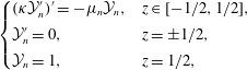 $$\begin{eqnarray}\left\{\begin{array}{@{}ll@{}}(\unicode[STIX]{x1D705}{\mathcal{Y}}_{n}^{\prime })^{\prime }=-\unicode[STIX]{x1D707}_{n}{\mathcal{Y}}_{n},\quad & z\in [-1/2,1/2],\\ {\mathcal{Y}}_{n}^{\prime }=0,\quad & z=\pm 1/2,\\ {\mathcal{Y}}_{n}=1,\quad & z=1/2,\end{array}\right.\end{eqnarray}$$
for
 ${\mathcal{Z}}_{n}(z)$
and
 ${\mathcal{Y}}_{n}(z)$
. We choose the boundary conditions
 ${\mathcal{Z}}_{n},{\mathcal{Y}}_{n}=1$
at
 $z=1/2$
to normalise our eigenfunctions. The constants
 $z_{n}$
and
 $y_{n}$
can be calculated by numerical integration using the solutions.
We now consider a function
 $\boldsymbol{g}(\unicode[STIX]{x1D748})\in \mathbb{R}^{m}$
, where
 $\unicode[STIX]{x1D748}\in \mathbb{R}^{m}$
for some positive integer
 $m$
. We seek the roots of
 $\boldsymbol{g}$
, i.e. the solutions
 $\unicode[STIX]{x1D748}=\unicode[STIX]{x1D748}^{\ast }$
satisfying
 $\boldsymbol{g}(\unicode[STIX]{x1D748})=\mathbf{0}$
. We can solve for
 $\unicode[STIX]{x1D748}^{\ast }$
numerically using the Newton–Raphson iteration,
 $$\begin{eqnarray}\unicode[STIX]{x1D748}_{n+1}=\unicode[STIX]{x1D748}_{n}-\left[\frac{\unicode[STIX]{x2202}\boldsymbol{g}}{\unicode[STIX]{x2202}\unicode[STIX]{x1D748}}(\unicode[STIX]{x1D748}_{n})\right]^{-1}\boldsymbol{\cdot }\boldsymbol{g}(\unicode[STIX]{x1D748}_{n}),\end{eqnarray}$$
for some suitable chosen initial guess
 $\unicode[STIX]{x1D748}_{0}$
. The Jacobian matrix, given by
 $$\begin{eqnarray}\left[\frac{\unicode[STIX]{x2202}\boldsymbol{g}}{\unicode[STIX]{x2202}\unicode[STIX]{x1D748}}\right]_{ij}=\frac{\unicode[STIX]{x2202}g_{i}}{\unicode[STIX]{x2202}\unicode[STIX]{x1D70E}_{j}},\end{eqnarray}$$
can be approximated numerically to second order by
 $$\begin{eqnarray}\left[\frac{\unicode[STIX]{x2202}\boldsymbol{g}}{\unicode[STIX]{x2202}\unicode[STIX]{x1D748}}\right]_{ij}\approx \frac{1}{2\unicode[STIX]{x1D6FF}}[g_{i}(\unicode[STIX]{x1D748}+\unicode[STIX]{x1D6FF}\boldsymbol{e}_{j})-g_{i}(\unicode[STIX]{x1D748}-\unicode[STIX]{x1D6FF}\boldsymbol{e}_{j})],\end{eqnarray}$$
for some small
 $\unicode[STIX]{x1D6FF}$
requiring
 $2m$
evaluations of
 $\boldsymbol{g}$
. We now iterate (C 4) until a suitable convergence condition is met;
 $\unicode[STIX]{x1D748}_{0}$
is chosen near the root such that the method converges. We say that the method has converged once
 $$\begin{eqnarray}|\boldsymbol{g}(\unicode[STIX]{x1D748}_{n})|<\unicode[STIX]{x1D716}^{\ast },\end{eqnarray}$$
for small parameter
 $\unicode[STIX]{x1D716}^{\ast }$
.
We now write (C 1)–(C 3) as first-order systems of the form
 $$\begin{eqnarray}\boldsymbol{y}^{\prime }=\boldsymbol{h}(\boldsymbol{y},z),\end{eqnarray}$$
for solution vector
 $\boldsymbol{y}$
, function
 $\boldsymbol{h}$
and parameter
 $z$
. We write (C 1) as
 $$\begin{eqnarray}\left(\begin{array}{@{}c@{}}K_{0}\\ \unicode[STIX]{x1D708}K_{0}^{\prime }\\ (\unicode[STIX]{x1D708}K_{0}^{\prime })^{\prime }\\ \unicode[STIX]{x1D708}(\unicode[STIX]{x1D708}K_{0}^{\prime })^{\prime \prime }\end{array}\right)^{\prime }=\left(\begin{array}{@{}c@{}}[\unicode[STIX]{x1D708}K_{0}^{\prime }]/\unicode[STIX]{x1D708}\\ (\unicode[STIX]{x1D708}K_{0}^{\prime })^{\prime }\\ \hspace{0.0pt}[\unicode[STIX]{x1D708}(\unicode[STIX]{x1D708}K_{0}^{\prime })^{\prime \prime }]/\unicode[STIX]{x1D708}\\ -K_{0}-\unicode[STIX]{x1D701}\end{array}\right),\end{eqnarray}$$
with initial condition
 $$\begin{eqnarray}\left(\begin{array}{@{}c@{}}K_{0}\\ \unicode[STIX]{x1D708}K_{0}^{\prime }\\ (\unicode[STIX]{x1D708}K_{0}^{\prime })^{\prime }\\ \unicode[STIX]{x1D708}(\unicode[STIX]{x1D708}K_{0}^{\prime })^{\prime \prime }\end{array}\right)=\left(\begin{array}{@{}c@{}}\unicode[STIX]{x1D70E}_{1}\\ 0\\ \unicode[STIX]{x1D70E}_{2}\\ 0\end{array}\right),\end{eqnarray}$$
at
 $\unicode[STIX]{x1D701}=-1/\sqrt{4E}$
. We now integrate from
 $\unicode[STIX]{x1D701}=-1/\sqrt{4E}$
to
 $\unicode[STIX]{x1D701}=1/\sqrt{4E}$
using a Runge–Kutta method and define
 $$\begin{eqnarray}\boldsymbol{g}(\unicode[STIX]{x1D70E}_{1},\unicode[STIX]{x1D70E}_{2})=\left.\left(\begin{array}{@{}c@{}}\unicode[STIX]{x1D708}K_{0}^{\prime }\\ \unicode[STIX]{x1D708}(\unicode[STIX]{x1D708}K_{0}^{\prime })^{\prime \prime }\end{array}\right)\right|_{\unicode[STIX]{x1D701}=1/\sqrt{4E}}.\end{eqnarray}$$
We can see that finding a numerical solution for
 $K_{0}$
requires us to calculate the correct initial conditions
 $(\unicode[STIX]{x1D70E}_{1},\unicode[STIX]{x1D70E}_{2})$
such that the boundary conditions at
 $\unicode[STIX]{x1D701}=1/\sqrt{4E}$
are satisfied. These conditions correspond to
 $\boldsymbol{g}=\mathbf{0}$
, so we can solve for
 $(\unicode[STIX]{x1D70E}_{1},\unicode[STIX]{x1D70E}_{2})$
iteratively using (C 4). The solution for
 $K_{0}$
is given by the solution using the value of
 $\unicode[STIX]{x1D748}_{n}$
once the convergence condition has been met.
The vertical structure function,
 $K_{0}$
, as a function of
 $z$
for
 $E=1$
(a), 0.1 (b), 0.01 (c) and 0.001 (d) and
 $\unicode[STIX]{x1D708}=11/8-9/2z^{2}$
.
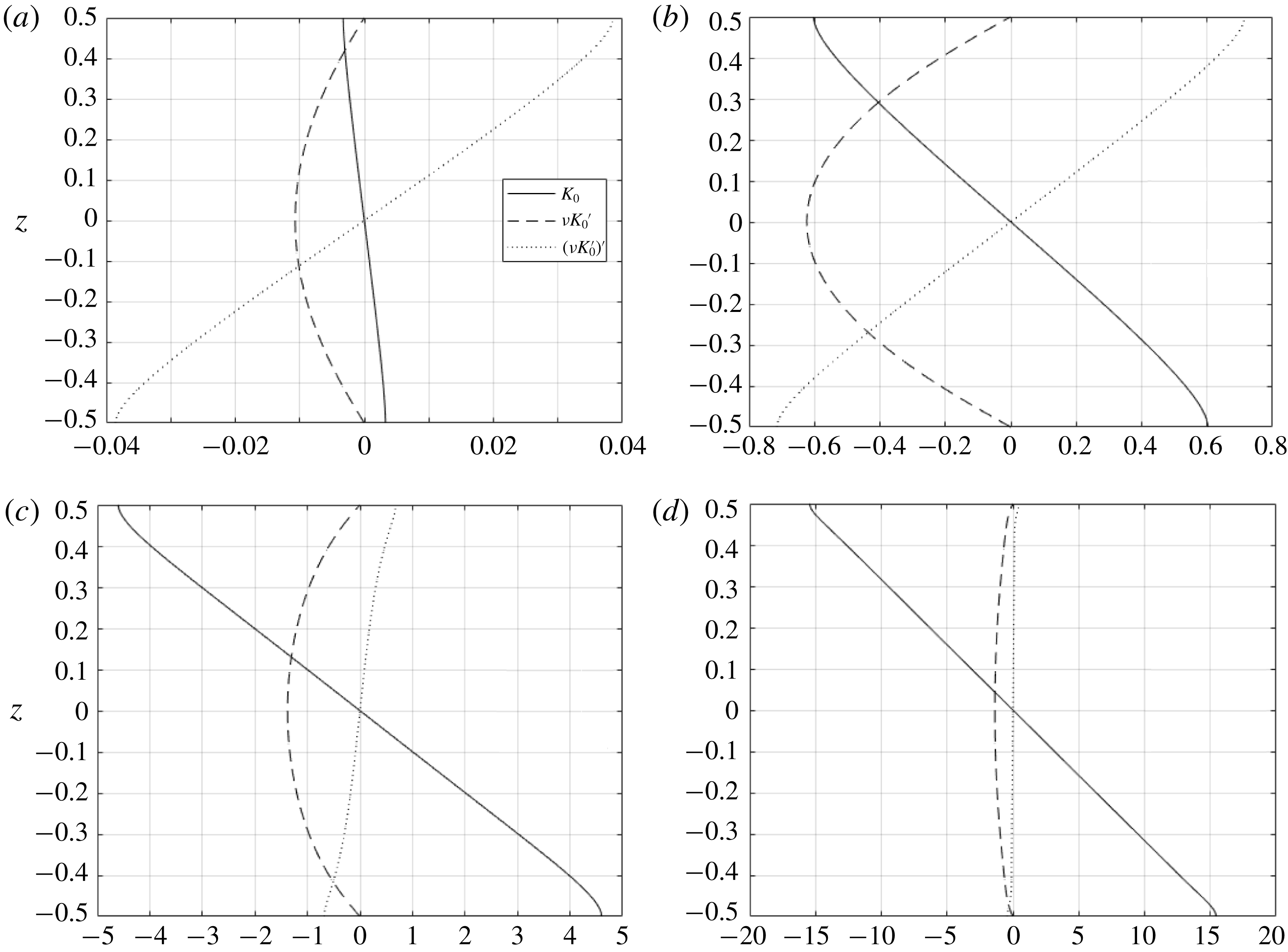
The vertical structure function,
 $K_{0}$
, as a function of
 $z$
for
 $E=1$
(a), 0.1 (b), 0.01 (c) and 0.001 (d) and
 $\unicode[STIX]{x1D708}=1$
.
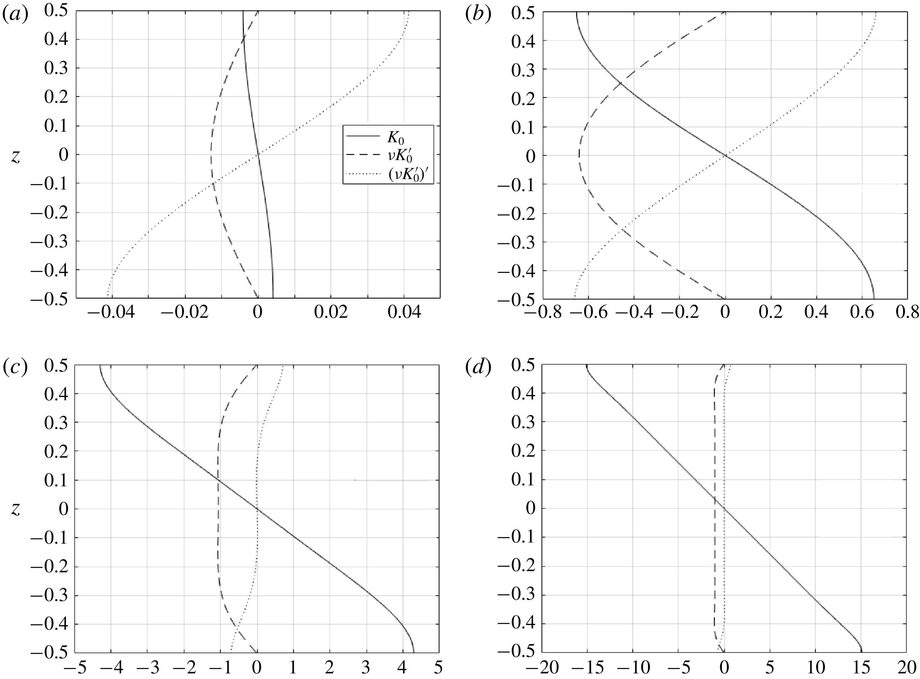
Plots of (a)
 ${\mathcal{Z}}_{n}$
for
 $\unicode[STIX]{x1D708}=1$
and
 $n\in \{0,1,2,3\}$
, (b)
 ${\mathcal{Z}}_{n}$
for
 $\unicode[STIX]{x1D708}=1$
and
 $n\in \{4,5,6,7\}$
, (c)
 ${\mathcal{Z}}_{n}$
for
 $\unicode[STIX]{x1D708}=11/8-9/2z^{2}$
and
 $n\in \{0,1,2,3\}$
, and (d)
 ${\mathcal{Z}}_{n}$
for
 $\unicode[STIX]{x1D708}=11/8-9/2z^{2}$
and
 $n\in \{4,5,6,7\}$
. We note that if
 $\unicode[STIX]{x1D705}=\unicode[STIX]{x1D708}$
, then
 ${\mathcal{Y}}_{n}={\mathcal{Z}}_{n}$
.

We now write (C 2) and (C 3) as
 $$\begin{eqnarray}\left(\begin{array}{@{}c@{}}{\mathcal{Z}}_{n}\\ \unicode[STIX]{x1D708}{\mathcal{Z}}_{n}^{\prime }\\ {\mathcal{Y}}_{n}\\ \unicode[STIX]{x1D705}{\mathcal{Y}}_{n}^{\prime }\end{array}\right)^{\prime }=\left(\begin{array}{@{}c@{}}[\unicode[STIX]{x1D708}{\mathcal{Z}}_{n}^{\prime }]/\unicode[STIX]{x1D708}\\ -\unicode[STIX]{x1D706}_{n}{\mathcal{Z}}_{n}\\ \hspace{0.0pt}[\unicode[STIX]{x1D705}{\mathcal{Y}}_{n}^{\prime }]/\unicode[STIX]{x1D705}\\ -\unicode[STIX]{x1D707}_{n}{\mathcal{Y}}_{n}\end{array}\right),\end{eqnarray}$$
with initial condition
 $$\begin{eqnarray}\left(\begin{array}{@{}c@{}}{\mathcal{Z}}_{n}\\ \unicode[STIX]{x1D708}{\mathcal{Z}}_{n}^{\prime }\\ {\mathcal{Y}}_{n}\\ \unicode[STIX]{x1D705}{\mathcal{Y}}_{n}^{\prime }\end{array}\right)=\left(\begin{array}{@{}c@{}}1\\ 0\\ 1\\ 0\end{array}\right)\end{eqnarray}$$
at
 $z=1/2$
and integrate backwards in
 $z$
. In order to satisfy the boundary conditions at
 $z=-1/2$
, we define
 $$\begin{eqnarray}\boldsymbol{g}(\unicode[STIX]{x1D70E}_{1},\unicode[STIX]{x1D70E}_{2})=\left.\left(\begin{array}{@{}c@{}}\unicode[STIX]{x1D708}{\mathcal{Z}}_{n}^{\prime }\\ \unicode[STIX]{x1D705}{\mathcal{Y}}_{n}^{\prime }\end{array}\right)\right|_{z=-1/2},\end{eqnarray}$$
where
 $(\unicode[STIX]{x1D70E}_{1},\unicode[STIX]{x1D70E}_{2})=(\unicode[STIX]{x1D706}_{n},\unicode[STIX]{x1D707}_{n})$
, and take
 $\unicode[STIX]{x1D748}$
such that
 $\boldsymbol{g}=\mathbf{0}$
. Therefore, the solution
 $\unicode[STIX]{x1D748}=\unicode[STIX]{x1D748}^{\ast }$
determines the eigenvalues, so we expect the components of
 $\boldsymbol{g}$
to be oscillatory with infinitely many positive roots. We note that the first component of
 $\boldsymbol{g}$
depends only on
 $\unicode[STIX]{x1D706}_{n}$
, while the second depends only on
 $\unicode[STIX]{x1D707}_{n}$
. We can plot
 $g_{1}(\unicode[STIX]{x1D706}_{n})$
and
 $g_{2}(\unicode[STIX]{x1D707}_{n})$
and use the plots to determine approximate values for the eigenvalues; these can be taken as starting values,
 $\unicode[STIX]{x1D748}_{0}$
, in a Newton–Raphson iteration using (C 4). The solutions and eigenvalues are given once the method has converged.
We now consider a K-profile parametrisation (KPP) (Large et al. Reference Large, McWilliams and Doney1994) with
 $\unicode[STIX]{x1D708}=\unicode[STIX]{x1D705}$
, where
 $\unicode[STIX]{x1D708}$
is given by
 $$\begin{eqnarray}\unicode[STIX]{x1D708}={\textstyle \frac{11}{8}}-{\textstyle \frac{9}{2}}z^{2}.\end{eqnarray}$$
Numerical solutions for
 $K_{0}$
with
 $E=1$
, 0.1, 0.01 and 0.001 are shown in figure 10. We can see that the upwelling, which is proportional to
 $\unicode[STIX]{x1D708}K_{0}^{\prime }$
, is stronger for smaller
 $E$
, and, in the small-
 $E$
limit, the along-front velocity, which is proportional to
 $K_{0}^{\prime }$
, approaches the linear thermal wind profile. The cross-front velocity, proportional to
 $(\unicode[STIX]{x1D708}K_{0}^{\prime })^{\prime }$
, is greatest at the surface and for small
 $E$
is confined to thin boundary layers near the surfaces.
Figure 11 shows the solutions for
 $K_{0}$
with
 $E=1$
, 0.1, 0.01 and 0.001 in the case where
 $\unicode[STIX]{x1D708}=1$
. We can see that the form of the solutions is similar to the KPP case, with a high horizontal surface velocity and strong upwelling in the centre of the vertical domain. For small
 $E$
, the boundary layers are thicker for the constant case as the viscosity in this region is higher and the upwelling is approximately constant throughout the vertical domain. In both cases, the along-front velocity approaches the linear thermal wind profile for small
 $E$
.
Figure 12 shows a comparison between the first eight vertical harmonics,
 ${\mathcal{Z}}_{n}$
, for the constant and KPP viscosity profiles. We note that
 ${\mathcal{Y}}_{n}={\mathcal{Z}}_{n}$
when
 $\unicode[STIX]{x1D705}=\unicode[STIX]{x1D708}$
. We can see that the magnitude of the oscillations in the interior is smaller for the KPP case as the viscosity is higher here compared with the region near the boundary; we can think of this as stronger damping.



