2. Quantile-based weighted residual extropy

Throughout the paper, we assume that the random variable $X$ is defined on $S_X$ and is absolutely continuous, with the cumulative distribution function (CDF) $F$ assumed to be strictly increasing, continuous, and differentiable, the density satisfies $f \in L^2(\mathbb{R})$, the weight function $w(x)$ is non-negative and integrable and defined on $S_X$, and the quantile function $Q(u)$ is differentiable.

The quantile function of a random variable $X$, with CDF $F$, is defined as

(4)\begin{equation} Q(p) = F^{-1}(p) = \inf\{x \in \mathbb{R} : F(x) \geq p\}, \quad 0 \lt p \lt 1. \end{equation}

An elegant example of a continuous probability distribution that lacks a closed-form CDF but possesses an explicit, closed-form quantile function is the Tukey Lambda distribution (Tukey [Reference Tukey40]).

Instead of being defined via its density or distribution function, the Tukey Lambda distribution is defined directly through its quantile function $Q(p)$, where $p \in [0, 1]$ represents the cumulative probability as

(5)\begin{equation} Q(p) = \frac{p^\lambda - (1-p)^\lambda}{\lambda} \end{equation}

Here, $\lambda \in \mathbb{R}$ is a shape parameter. Despite lacking an explicit CDF, this quantile-defined family is highly valued in statistical modeling and Monte Carlo simulations due to its structural simplicity and ability to approximate various standard distributions. Hence, quantile-based reliability analysis of weighted extropy is a useful study.

Let $ X $ be a continuous random variable with pdf $ f(\cdot) $. Then, the composition $ f(Q(p)) $ is referred to as the density quantile function, while its derivative $ q(p) = \frac{d}{dp} Q(p) $ is known as the quantile density function (see Parzen [Reference Parzen32]).

From the relationship $ F(Q(p)) = p $, it follows, by differentiation with respect to $ p $, that (see Krishnan et al. [Reference Krishnan, Sunoj and Sankaran25])

(6)\begin{equation} q(p) f(Q(p)) = 1. \end{equation}

Equation (6) holds under the assumption that the distribution function $F$ is strictly increasing and differentiable, with $f(Q(p)) \gt 0$ for all $p \in (0,1)$.

This identity connects the quantile function with the corresponding density function and serves as a key tool in developing quantile-based information measures.

A particularly important quantity in reliability analysis is the hazard quantile function, defined as

(7)\begin{equation} H(p) = h(Q(p)) = \frac{1}{(1 - p) q(p)}, \quad 0 \lt p \lt 1. \end{equation}

This definition requires that the quantile function $Q(p)$ is differentiable on $(0,1)$, where $ h(t) = \frac{f(t)}{\bar{F}(t)} $ denotes the traditional hazard rate function of $ X $, and $ \bar{F}(t) = 1 - F(t) $ is the survival function. The hazard quantile function $H(p)$ represents the instantaneous risk at the $p$-th quantile.

The mean residual life (MRL) function describes the expected remaining lifetime of a component that has survived up to a specific time $ x $. It is defined as

(8)\begin{equation} m(x) = \mathbb{E}(X - x \mid X \gt x) = \frac{1}{1 - F(x)} \int_x^{u_X} (1 - F(t)) \, dt, \end{equation}

where $ F(x) $ is the CDF of the lifetime variable $ X $. Building on this, the mean residual quantile function evaluates the MRL at a specific quantile level. It is given by

(9)\begin{equation} M(u) = m(Q(u)) = \frac{1}{1 - u} \int_u^1 (1 - p) q(p) \, dp= \frac{1}{1 - u} \int_u^1 (Q(p) - Q(u)) \, dp, \end{equation}

where $ Q(u) $ is the quantile function corresponding to $ F(x) $, and $ q(p) = \frac{d}{dp}Q(p) $ is its derivative. This quantile-based formulation of the MRL is particularly useful in reliability analysis and survival studies for interpreting remaining life in terms of distributional quantiles.

It is worth noting that $ H(p) $ uniquely determines the quantile function $ Q(p) $ (see Nair and Sankaran [Reference Nair and Sankaran30]). This makes $ H(p) $ a fundamental tool for characterizing lifetime distributions in the quantile domain.

Krishnan et al. [Reference Krishnan, Sunoj and Sankaran25] investigated various properties of extropy and its associated measures through the lens of quantile functions. The study explored ordering relationships related to quantile-based residual extropy.

Using the identity $F(Q(p)) = p$, differentiation with respect to $p$ yields $ f(Q(p))\,Q'(p) = 1,$ which implies $f(Q(p)) = \frac{1}{q(p)}$, where $q(p) = Q'(p)$ is the quantile density function. The quantile-based weighted extropy with weight $w_1(x)\geq 0$ is defined as

\begin{align*} L^{w_1}(X)&=-\frac{1}{2} \int_{0}^{1}w_1(Q(p)) f^2(Q(p))dQ(p)\\ &=-\frac{1}{2} \int_{0}^{1}w_1(Q(p)) \left(q(p)\right)^{-1}dp\\ &=-\frac{1}{2}\int_{0}^{1}w_1(Q(p)) (1-p) H(p) dp, \end{align*}

here $L^{w_1}(X)$ is the quantile version of weighted extropy. It measures the uncertainty of random variable $X$, which is obtained either using the quantile density function or the hazard quantile function. When $w_1(x)=\left(F(x)\right)^{\alpha-1}$, then we denote $L^{w_1}(X)$ as $L^{(\alpha)}(X)$. The expression for $L^{\alpha}(X)$ is obtained as

\begin{align*} L^{(\alpha)}(X)&=-\frac{1}{2} \int_{0}^{1} p^{\alpha-1} f^2(Q(p))dQ(p)\\ &=-\frac{1}{2} \int_{0}^{1} p^{\alpha-1} \left(q(p)\right)^{-1}dp\\ &=-\frac{1}{2}\int_{0}^{1} p^{\alpha-1} (1-p) H(p) dp. \end{align*}

Table 1 lists several standard quantile functions together with their associated quantile-based weighted extropy $L^{(\alpha)}(X)$ functions. Let $X$ and $Y$ be random variables with Pareto II $(c=1,\ \gamma=1)$ and Rescaled beta $(c=1,\ R=3)$, respectively. Then $L(X)=L(Y)=-1/6$, but $L^{(2)}(X)=-1/24$ and $L^{(2)}(Y)=-1/12$. Thus, in this case, quantile version of extropies are the same, but the quantile version of weighted extropies are different for $\alpha=2$. Therefore, the quantile version of weighted extropies can also play a role as a measure of uncertainty.

Table 1.

Quantile-based weighted extropy for some quantile functions.

Table 1 Long description

Four columns give distribution name, probability density function, quantile function, and L alpha of X. Rows cover Exponential with parameter lambda, Pareto II with parameters gamma and c, Rescaled Beta with parameters c and R, Generalized Pareto with parameters a and b, Power with parameters gamma and beta, Uniform with parameters a and b, and Davies with parameters c, lambda 1, and lambda 2. For Exponential, the density is defined for x greater than zero, and L alpha of X is written using lambda and the beta function. Pareto II and Generalized Pareto list densities with a one plus x over a scale term raised to a negative power, and their L alpha of X entries use the beta function with parameter combinations that include c or a. Rescaled Beta and Power specify support between zero and an upper bound, R or gamma, and their L alpha of X entries include c over R or a rational expression in beta and gamma. Uniform gives a constant density between a and b, a linear quantile function in u, and an L alpha of X term proportional to one over alpha times b minus a. Davies provides a density written in terms of u with parameters c, lambda 1, and lambda 2, a quantile function using powers of u and one minus u, and an L alpha of X expression that continues onto a second line with a beta function term multiplied by a hypergeometric function.

In Table 1, $B(a, b)$ represents complete Beta function defined as

\begin{equation*} B(a, b) = \int_0^1 p^{a - 1}(1 - p)^{b - 1} \, dp, \end{equation*}

and the symbol ${}_2F_1(a,b;c;z)$ represents the Gauss hypergeometric function, defined as:

\begin{equation*} {}_2F_1(a,b;c;z) = \sum_{n=0}^{\infty} \frac{(a)_n\, (b)_n}{(c)_n} \frac{z^n}{n!} \end{equation*}

where

1. (i) $(a)_n$ is the Pochhammer symbol or rising factorial, defined by:

   \begin{equation*} (a)_0 = 1,\quad (a)_n = a(a+1)\cdots(a+n-1),\quad \text{for } n \geq 1 \end{equation*}

2. (ii) $a, b, c, z$ can be real or complex numbers, with the restriction that $c \notin \mathbb{Z}_{\leq 0}$.

3. (iii) The series converges absolutely for $|z| \lt 1$, and may also converge at $|z| = 1$ under suitable conditions on $a, b, c$.

The quantile-based weighted extropy of $X_t$, denoted by $L_Q^{w_1}(u)$, measures the magnitude-sensitive uncertainty of the residual lifetime beyond quantile $u$ and is defined as

(10)\begin{align} L_Q^{w_1}(u) &= -\frac{1}{2(1-u)^2} \int_u^1 w_1\bigl(Q(p)\bigr)f^2\bigl(Q(p)\bigr)\,dQ(p)\\ &= -\frac{1}{2(1-u)^2} \int_u^1 w_1\bigl(Q(p)\bigr)\bigl(q(p)\bigr)^{-1}\,dp\\ &= -\frac{1}{2(1-u)^2} \int_u^1 w_1\bigl(Q(p)\bigr)(1-p)H(p)\,dp. \end{align}

Now differentiating (10) with respect to $u$, using Leibniz’s rule, taking into account the dependence of both the integral limits and the factor $(1-u)^2$ on $u$, we have

(11)\begin{equation} \left(L_{Q}^{w_1}(u)\right)^\prime=\frac{w_1(Q(u)) H(u)}{2(1-u)}+\frac{2L_{Q}^{w_1}(u)}{(1-u)} \end{equation}

equivalentely

(12)\begin{equation} q(u)=w_1(Q(u))\left(2(1-u)^2\left(L_{Q}^{w_1}(u)\right)^\prime-4(1-u)L_{Q}^{w_1}(u)\right)^{-1} \end{equation}

The above inversion formula holds provided that $ 2(1-u)^2\left(L_{Q}^{w_1}(u)\right)^\prime-4(1-u)L_{Q}^{w_1}(u) \neq 0. $ The above expression determines $L_{Q}^{w_1}(u)$ uniquely using the quantile density function through this simple relationship, although the extropy function does not have such a relationship.

When $w_1(x)=\left(F(x)\right)^{\alpha-1}$, then we denote $L_Q^{w_1}(X)$ as $L_Q^{(\alpha)}(X)$. The expression for $L_Q^{\alpha}(X)$ is obtained as

\begin{align*} L_Q^{w^1}(u) &= -\frac{1}{2(1-u)^2} \int_u^1 w_1(Q(p))f^2(Q(p))\,dQ(p)\\ &= -\frac{1}{2(1-u)^2} \int_u^1 w_1(Q(p))\left(q(p)\right)^{-1}\,dp\\ &= -\frac{1}{2(1-u)^2} \int_u^1 w_1(Q(p))(1-p)H(p)\,dp. \end{align*}

In Table 2, $B_u(a, b)$ represents incomplete Beta function defined as

\begin{equation*} B_u(a, b) = \int_u^1 p^{a - 1}(1 - p)^{b - 1} \, dp. \end{equation*}

Table 2.

Quantile-based weighted residual extropy $ L_Q^{(\alpha)}(u) $ using incomplete Beta function representations.

Table 2 Long description

Columns are labeled, Distribution, Quantile Function Q of u, and L Q of alpha of u. Each row pairs a named distribution with its quantile function and an expression for L Q of alpha of u written using an incomplete Beta function. Exponential gives a log based quantile with rate parameter lambda greater than zero, and an L Q term with lambda times an incomplete Beta function with parameters alpha and two. Pareto II gives a quantile using gamma and c greater than zero, and an L Q term with c over gamma and an incomplete Beta function with parameters alpha and two plus one over c. Rescaled Beta gives a quantile using R and c greater than zero, and an L Q term with c over R and an incomplete Beta function with parameters alpha and two minus one over c. Generalized Pareto gives a quantile using a greater than minus one and b greater than zero, and an L Q term with a plus one over b and an incomplete Beta function with parameters alpha and two plus a over a plus one. Power gives a quantile using gamma and beta greater than zero, and an L Q term with beta over gamma and an incomplete Beta function with parameters alpha plus one minus one over beta and one. Uniform gives a linear quantile from a to b with a less than b, and an L Q term with one over b minus a and an incomplete Beta function with parameters alpha and one. Davies gives a quantile using c, lambda one, and lambda two greater than zero, and an L Q term with one over c and an incomplete Beta function with parameters alpha minus lambda one plus one and lambda two plus two.

Theorem 1. Let random variable $X$ follows a distribution with quantile density function

(13)\begin{equation}q(u)=ku^\delta (1-u)^{-(A+\delta)}, \ k \gt 0,\ A,\delta \in \mathbb{R}, \ u\in (0,1),\end{equation}

if and only if

\begin{equation*}(1-u)^2L_{Q}^{(\alpha)}(u)=-k_1\tilde{B}_u(a,b),\end{equation*}

where $k_1 \gt 0$ and $\tilde{B}_u(a,b)=\int_{u}^{1}p^{a-1}(1-p)^{b-1}dp$ denote the incomplete beta function.

Proof. Since the proof of the if part is straightforward, we only prove the only-if part. Assume $(1-u)^2L_{Q}^{(\alpha)}(u)=-k_1\tilde{B}_u(a,b)$ holds. On differentaiting both sides with respect to $u$, we have

\begin{equation*}(1-u)^2\left(L_{Q}^{(\alpha)}(u)\right)^\prime-2(1-u)L_{Q}^{(\alpha)}(u)=k_1u^{a-1}(1-u)^{b-1}.\end{equation*}

Now from (12) with $w(x)=\left(F(x)\right)^{\alpha-1}$ and using above equation, we obtain the quantile model (13). $\square$

The family of distributions (13) contains some important probability distributions; one may refer to Krishnan et al. [Reference Krishnan, Sunoj and Sankaran25] and Nair et al. [Reference Nair, Sankaran and Balakrishnan31] for details of these.

The proof of the following theorem is straightforward from (11), hence omitted.

Proof. From Eq. (11), we have

\begin{equation*} \left(L^{w_1}_{Q_X}(u)\right)' = \frac{w_1(Q_X(u)) H_X(u)}{2(1-u)} + \frac{2L^{w_1}_{Q_X}(u)}{1-u}. \end{equation*}

Multiplying both sides by $(1-u)$, we obtain

\begin{equation*} (1-u)\left(L^{w_1}_{Q_X}(u)\right)' = \frac{w_1(Q_X(u)) H_X(u)}{2} + 2L^{w_1}_{Q_X}(u). \end{equation*}

Rearranging terms gives

\begin{equation*} 2L^{w_1}_{Q_X}(u) = (1-u)\left(L^{w_1}_{Q_X}(u)\right)' - \frac{w_1(Q_X(u)) H_X(u)}{2}. \end{equation*}

Hence,

\begin{equation*} L^{w_1}_{Q_X}(u) = \frac{1-u}{2}\left(L^{w_1}_{Q_X}(u)\right)' - \frac{w_1(Q_X(u)) H_X(u)}{4}. \end{equation*}

Now consider two cases.

Case 1: If $L^{w_1}_{Q_X}(u)$ is increasing in $u$, then

\begin{equation*} \left(L^{w_1}_{Q_X}(u)\right)' \ge 0. \end{equation*}

Since $1-u \gt 0$ for $u \in (0,1)$, we get

\begin{equation*} \frac{1-u}{2}\left(L^{w_1}_{Q_X}(u)\right)' \ge 0. \end{equation*}

Therefore,

\begin{equation*} L^{w_1}_{Q_X}(u) \ge -\frac{w_1(Q_X(u)) H_X(u)}{4}. \end{equation*}

Case 2: If $L^{w_1}_{Q_X}(u)$ is decreasing in $u$, then

\begin{equation*} \left(L^{w_1}_{Q_X}(u)\right)' \le 0. \end{equation*}

Thus,

\begin{equation*} \frac{1-u}{2}\left(L^{w_1}_{Q_X}(u)\right)' \le 0, \end{equation*}

and consequently,

\begin{equation*} L^{w_1}_{Q_X}(u) \le -\frac{w_1(Q_X(u)) H_X(u)}{4}. \end{equation*}

This completes the proof.

Proof. Using Theorem 3.B.13(b) of Shaked and Shanthikumar [Reference Shaked and Shanthikumar42], $X\le_{disp} Y$ implies that $X\ge_{st} Y$. Hence $Q_X(u) \ge Q_Y(u)$ for all $u\in (0,1)$. Since $w_1(x)$ is increasing and $w_2(x)\leq w_1(x)$, hence

(14)\begin{equation} w_1(Q_X(u)) \ge w_1(Q_Y(u))\ge w_2(Q_Y(u)). \end{equation}

Now, since $X\leq_{disp} Y$ and using (14), we have

(15)\begin{equation} w_1(Q_X(u)) \left(q_X(u)\right)^{-1}\geq w_2(Q_Y(u)) \left(q_Y(u)\right)^{-1}. \end{equation}

Using (10) and (15), we have

\begin{align*} L_{Q_X}^{w_1}(u)&=-\frac{1}{2(1-u)^2} \int_{u}^{1}w_1(Q_X(p)) \left(q_X(p)\right)^{-1}dp\\ &\leq -\frac{1}{2(1-u)^2} \int_{u}^{1}w_2(Q_Y(p)) \left(q_Y(p)\right)^{-1}dp\\ &=L_{Q_Y}^{w_2}(u) \end{align*}

Example 1. Let us consider $X\sim\operatorname{Exp}(1)$ and $Y\sim\operatorname{Exp}(0.5)$ with weight functions $w_1(x)=x+1, \text{and} \ \ w_2(x)=x.$ We obtain the explicit functions

\begin{equation*} {L_{Q_X}^{w_1}(u)=\frac14\log(1-u)-\frac38},\qquad {L_{Q_Y}^{w_2}(u)=\frac14\log(1-u)-\frac18}. \end{equation*}

We have $L_{Q_X}^{w_1}(u) \leq L_{Q_Y}^{w_2}(u)$ for all $u\in(0,1)$,

One may refer to Shaked and Shantikumar [Reference Shaked and Shanthikumar42] for details of convex transform order ( $\leq_c$), star order ( $\leq_{\star}$), superadditive order ( $\leq_{su}$), and dispersive order ( $\leq_{disp}$). In view of Theorem 3 and Lemma 1, the following result is obtained.

3. Weighted extropy of order statistics

Let $X_{i:n}$ denote the $i$th order statistic. The weighted extropy of $i$th order statistic with weight $w_1$ is given by

(16)\begin{equation} J(X_{i:n})=\frac{-1}{2}\int_{S_X}w_1(x)f_{i:n}^{2}(x)dx. \end{equation}

Now the quantile-based weighted extropy based on (16) is

\begin{align*} &L^{w_1}(X_{i:n})\\ &\ = -\frac{1}{2} \int_{0}^{1}w_1(Q(u)) \frac{(n!)^2}{((i-1)!)^2 ((n-i)!)^2} u^{2i-2} (1-u)^{2n-2i}\left(q(u)\right)^{-2}dQ(u)\\ &\ =-\frac{1}{2} \int_{0}^{1}w_1(Q(u)) \frac{(n!)^2}{((i-1)!)^2 ((n-i)!)^2} u^{2i-2} (1-u)^{2n-2i}\left(q(u)\right)^{-1}du. \end{align*}

In the following theorem, we study the property of quantile-bsed extropy of order statistics when the underlying iid random variables are symmetric.

Proof.

Let $X_1, \dots, X_n$ be a random sample from a distribution symmetric about $\mu$. Then the quantile function satisfies

\begin{equation*} Q(1-u) = 2\mu - Q(u), \quad 0 \lt u \lt 1. \end{equation*}

Differentiating both sides with respect to $u$, we obtain

\begin{equation*} q(1-u) = q(u), \end{equation*}

so the quantile density function is symmetric.

Now recall that the quantile-based weighted extropy of the $i$-th order statistic is

\begin{equation*} L_{w_1}(X_{i:n}) = -\frac{1}{2} \int_0^1 w_1(Q(u)) \frac{(n!)^2}{((i-1)!)^2((n-i)!)^2} u^{2i-2}(1-u)^{2n-2i} (q(u))^{-1} \, du. \end{equation*}

Let

\begin{equation*} C_{i,n} = \frac{(n!)^2}{((i-1)!)^2((n-i)!)^2}. \end{equation*}

Then

\begin{equation*} L_{w_1}(X_{i:n}) = -\frac{1}{2} \int_0^1 w_1(Q(u)) C_{i,n} u^{2i-2}(1-u)^{2n-2i} (q(u))^{-1} \, du. \end{equation*}

Now consider $L_{w_1}(X_{n-i+1:n})$:

\begin{equation*} L_{w_1}(X_{n-i+1:n}) = -\frac{1}{2} \int_0^1 w_1(Q(u)) C_{n-i+1,n} u^{2n-2i}(1-u)^{2i-2} (q(u))^{-1} \, du. \end{equation*}

Observe that

\begin{equation*} C_{n-i+1,n} = C_{i,n}. \end{equation*}

Now make the transformation $u = 1-v$. Then $du = -dv$, and the limits remain $(0,1)$. Using symmetry properties:

\begin{equation*} Q(1-v) = 2\mu - Q(v), \quad q(1-v) = q(v). \end{equation*}

Also,

\begin{equation*} (1-v)^{2n-2i} v^{2i-2} = v^{2i-2}(1-v)^{2n-2i}. \end{equation*}

Thus the integral for $L_{w_1}(X_{n-i+1:n})$ becomes identical to that of $L_{w_1}(X_{i:n})$.

Hence,

\begin{equation*} L_{w_1}(X_{i:n}) = L_{w_1}(X_{n-i+1:n}). \end{equation*}

This proves part (i).

For part (ii), define

\begin{equation*} \Delta L_{w_1}(X_{i:n}) = L_{w_1}(X_{i+1:n}) - L_{w_1}(X_{i:n}). \end{equation*}

Using part (i), we have

\begin{equation*} L_{w_1}(X_{i:n}) = L_{w_1}(X_{n-i+1:n}). \end{equation*}

Then

\begin{equation*} \Delta L_{w_1}(X_{n-i:n}) = L_{w_1}(X_{n-i+1:n}) - L_{w_1}(X_{n-i:n}). \end{equation*}

Replacing using symmetry,

\begin{equation*} = L_{w_1}(X_{i:n}) - L_{w_1}(X_{i+1:n}) = - \Delta L_{w_1}(X_{i:n}). \end{equation*}

Therefore,

\begin{equation*} \Delta L_{w_1}(X_{i:n}) = - \Delta L_{w_1}(X_{n-i+1:n}), \quad i=1,\dots,n-1. \end{equation*}

This completes the proof.

Let

\begin{align*} \phi_{2i-1:2n-1}(u)= \frac{(2n-1)!}{(2i-2)! (2n-2i)!} u^{2i-2} (1-u)^{2n-2i}, 0 \lt u \lt 1. \end{align*}

Then $\phi_{2i-1:2n-1}(u)$ represents the pdf of a beta-distributed random variable with parameters (2 $i-$1) and (2 $n-2i$+1); we denote this random variable by $B_{2i-1:2n-1}$.

Now we consider the quantile-based weighted residual extropy of the $i$th order statistic based on the random variable $X_t$ as

\begin{align*} L_{Q_{i:n}}^{w_1}(u) & =-\frac{1}{2} \int_{u}^{1}w_1(Q(p)) \frac{(n!)^2}{((i-1)!)^2 ((n-i)!)^2} p^{2i-2} (1-p)^{2n-2i}\left(q(p)\right)^{-1}dp.\\ &=-\frac{c_{i,n}(2i-1)}{4}\int_{u}^{1}w_1(Q(p))r\left(Q(p)\right)\phi_{2i:2n}(p)dp\\ &=-\frac{c_{i,n}(2i-1)}{4}P\left(M(B_{2i:2n}) \gt u\right), \end{align*}

where $c_{i,n}=\frac{\binom{2i-2}{i-1}\binom{2n-2i}{n-i}}{\binom{2n-1}{n-1}}$, $M(p)=w_1(Q(p))r\left(Q(p)\right)$ and $r(x)$ denote the reverse failure rate function of $X$. It is clear that $L_{Q_{i:n}}^{w_1}(u)$ is increasing in $u$.

Proof. The quantile-based weighted residual extropy of the $i$-th order statistic is given by

\begin{equation*} L^{w_1}_{Q_{i:n}}(u) = -\frac{1}{2} \int_u^1 w_1(Q(p)) \frac{(n!)^2}{((i-1)!)^2((n-i)!)^2} p^{2i-2}(1-p)^{2n-2i} (q(p))^{-1} \, dp. \end{equation*}

Let

\begin{equation*} C_{i,n} = \frac{(n!)^2}{((i-1)!)^2((n-i)!)^2}. \end{equation*}

Define

\begin{equation*} g(p) = w_1(Q(p)) C_{i,n} p^{2i-2}(1-p)^{2n-2i} (q(p))^{-1}. \end{equation*}

Since $w_1(Q(p)) \ge 0$, $q(p) \gt 0$, and the beta-type term $p^{2i-2}(1-p)^{2n-2i} \ge 0$, we have

\begin{equation*} g(p) \ge 0 \quad \text{for } p\in(0,1). \end{equation*}

Thus,

\begin{equation*} L^{w_1}_{Q_{i:n}}(u) = -\frac{1}{2} \int_u^1 g(p)\, dp. \end{equation*}

Now differentiate with respect to $u$ using Leibniz rule:

\begin{equation*} \frac{d}{du} L^{w_1}_{Q_{i:n}}(u) = -\frac{1}{2} \frac{d}{du} \left( \int_u^1 g(p)\, dp \right). \end{equation*}

Since

\begin{equation*} \frac{d}{du} \int_u^1 g(p)\, dp = - g(u), \end{equation*}

we obtain

\begin{equation*} \frac{d}{du} L^{w_1}_{Q_{i:n}}(u) = -\frac{1}{2}(-g(u)) = \frac{1}{2} g(u). \end{equation*}

Because $g(u) \ge 0$, it follows that

\begin{equation*} \frac{d}{du} L^{w_1}_{Q_{i:n}}(u) \ge 0. \end{equation*}

Therefore,

\begin{equation*} L^{w_1}_{Q_{i:n}}(u) \text{ is increasing in } u. \end{equation*}

This completes the proof.

The above theorem gives the correct general version of Theorem 17 of Krishnan et al. [Reference Krishnan, Sunoj and Sankaran25]. The following example justifies the above theorem and works as a counterexample to Theorem 17 of Krishnan et al. [Reference Krishnan, Sunoj and Sankaran25]. The following example shows that when $X$ has a decreasing density quantile function $f(Q(u))$, then $L_{Q_{1:n}}^{w_1}(u)$ may not be decreasing in $u\in(0,1)$.

Example 2. Consider power-Pareto $(c=\lambda_1=\lambda_2=1)$ distribution having quantile function $Q(u)=\frac{u}{1-u}$ and $w(x)=F(x)$, that is, $L_{Q_{i:n}}^{w_1}(u)=L_{Q_{i:n}}^{(1)}(u)=L_{Q_{i:n}}(u)$. Then the density quantile function $f(Q(u))=(1-u)^2$ is decreasing in $u\in (0,1)$. Now consider

\begin{align*} L_{Q_{1:2}}(u)&=-\frac{4}{2(1-u)^4}\int_{u}^{1}(1-p)^2(1-p)^2dp\\ &=-\frac{2}{5}(1-u). \end{align*}

Note that $L_{Q_{1:2}}(1/4)=-(6/20) \lt L_{Q_{1:2}}(1/2)=-(4/20)$ which is not decreasing in $u$.

4. Weighted cumulative residual extropy

In this section, we discuss weighted cumulative residual extropy using the distribution function and quantile approach. Weighted cumulative residual extropy of non-negative random variable $X$ with weight $w_1$ is given by

(17)\begin{equation} \xi^{w_1}(X)=-\frac{1}{2}\int_{0}^{\infty} w_1(x) \bar F^2(x)dx. \end{equation}

The quantile version of Eq. (17) is

(18)\begin{equation} \xi^{w_1}(X)=-\frac{1}{2}\int_{0}^{1}w_1\left(Q(p)\right) (1-p)^2q(p)dp. \end{equation}

The weighted cumulative residual extropy of the random variable $X_t$ with weight $w_1$ is given by

(19)\begin{equation} \Phi^{w_1}(X_t)=-\frac{1}{2}\int_{t}^{u_X}w_1(x) \left( \frac{\bar F^2(x)}{\bar F^2(t)}\right)dx. \end{equation}

The quantile version of Eq. (19) is

(20)\begin{equation} \Phi_Q^{w_1}(u)=-\frac{1}{2(1-u)^2}\int_{u}^{1}w_1\left(Q(p)\right) (1-p)^2q(p)dp. \end{equation}

Differentiating the above equation with respect to $u$, we have

(21)\begin{equation} q(u)=\frac{1}{w_1(Q(u))}\left(2(\Phi_Q^{w_1}(u))^{\prime}-\frac{4\Phi_Q^{w_1}(u)}{(1-u)}\right). \end{equation}

Proof. Since $X\le_{disp} Y$, therefore we have $q_Y(u)\ge q_X(u)$ for $u \in (0,1)$. Then, using Theorem 3.B.13(b) of Shaked and Shanthikumar [Reference Soni, Dewan and Jain38], $X\le_{disp} Y$ implies that $X\ge_{st} Y$. Hence $Q_X(u) \ge Q_Y(u)$ for all $u\in (0,1)$. Since $w_1$ is decreasing and $w_1(x)\leq w_2(x)$, then $w_1(Q_X(u)) \le w_1(Q_Y(u))\le w_2(Q_Y(u))$. Hence

(22)\begin{align} w_2(Q_Y(u))q_Y(u) \geq w_1(Q_X(u))q_X(u) \Rightarrow \int_u^1 w_2(Q_Y(p))q_Y(p)(1-p)^2\,dp \geq \int_u^1 w_1(Q_X(p))q_X(p)(1-p)^2\,dp \Rightarrow \Phi_{Q_X}^{w_1}(u) \geq \Phi_{Q_Y}^{w_2}(u). \end{align}

Hence the result.

Remark 1. Let $X$ be a non-negative absolutely continuous random variable with survival function $\bar{F}(x)$, and let $w(x) \geq 0$ for all $x \geq 0$. Then the weighted cumulative residual extropy

\begin{equation*} \xi_w(X) = -\frac{1}{2} \int_{S_X} w(x)\, \bar{F}^2(x)\, dx \leq 0. \end{equation*}

Example 3. Let $X \sim \text{Exponential}(\lambda)$ and choose $w(x) = 1$. Then $\bar{F}(x) = e^{-\lambda x}$ and:

\begin{equation*} \xi_w(X) = -\frac{1}{2} \int_0^\infty e^{-2\lambda x} dx = -\frac{1}{2} \cdot \frac{1}{2\lambda} = -\frac{1}{4\lambda}. \end{equation*}

Theorem 8. Let $X$ be a non-negative continuous random variable with quantile function $Q(u)$ and quantile density $q(u) = \frac{dQ(u)}{du}$. Then the quantile-based weighted cumulative residual extropy is given by

\begin{equation*} \xi^w(X) = -\frac{1}{2} \int_0^1 w(Q(u))\, (1 - u)^2\, q(u)\, du. \end{equation*}

Proof. Using the change of variable $x = Q(u)$ and $dx = q(u)\, du$, and noting that $\bar{F}(Q(u)) = 1 - u$, we substitute into the definition of $\xi^w(X)$,

\begin{equation*} \xi^w(X) = -\frac{1}{2} \int_0^\infty w(x) \bar{F}^2(x)\, dx = -\frac{1}{2} \int_0^1 w(Q(u))\, (1 - u)^2\, q(u)\, du. \end{equation*}

Example 4. Let $X \sim \text{Uniform}(0,1)$, so $Q(u) = u$, $q(u) = 1$, and choose $w(x) = x$. Then,

\begin{equation*} \xi^w(X) = -\frac{1}{2} \int_0^1 u(1 - u)^2\, du = -\frac{1}{2} \cdot \frac{1}{12} = -\frac{1}{24}. \end{equation*}

Theorem 9. Let $\Phi^w_{Q}(u) = -\frac{1}{2(1 - u)^2} \int_u^1 w(Q(p)) (1 - p)^2 q(p)\, dp$ be the residual form of WCRE. Then the quantile density function $q(u)$ satisfies

\begin{equation*} q(u) = \frac{2\, \Phi_Q^{w\,\prime}(u) - \frac{4}{1 - u} \Phi^w_{Q}(u)}{w(Q(u))}. \end{equation*}

Proof. Differentiate both sides of the definition of 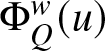$\Phi^w_{Q}(u)$ with respect to $u$ using Leibniz’s rule, and rearranging terms gives us the required expression.

Example 5. Let $w(x)=1$ and $\Phi^w_Q(u)=-\frac14(1-u)^2.$ Then $ \Phi_Q^{w\,\prime}(u)=\frac12(1-u). $ By Theorem 9,

\begin{equation*} q(u) = 2\Phi_Q^{w\,\prime}(u)-\frac{4}{1-u}\Phi^w_Q(u) =2(1-u). \end{equation*}

Hence, $Q(u)=2u-u^2,$ which is the quantile function of $ X\sim\operatorname{Beta}\left(1,\frac12\right).$ Thus, $q(u)=Q'(u)=2(1-u)$, verifying Theorem 9.

Example 6. Let $X\sim\mathrm{Uniform}(0,1)$ and $w(x)=1$. Then the quantile function and quantile density are

\begin{equation*} Q(u)=u,\qquad q(u)=Q'(u)=1,\qquad 0 \lt u \lt 1. \end{equation*}

From the definition of $\Phi_Q^w(u)$, we have

\begin{equation*} \begin{aligned} \Phi_Q^w(u) &= -\frac{1}{2(1-u)^2} \int_u^1 (1-p)^2q(p)\,dp= -\frac{1-u}{6}. \end{aligned} \end{equation*}

Therefore, $\Phi_Q^{w\,\prime}(u)=\frac{1}{6}.$ Now, using the result of Theorem 9,

\begin{equation*} \begin{aligned} q(u) &= \frac{ 2\Phi_Q^{w\,\prime}(u) -\dfrac{4}{1-u}\Phi_Q^w(u) }{ w(Q(u)) }=1. \end{aligned} \end{equation*}

On the other hand, directly from the quantile function $Q(u)=u$, we have $ q(u)=Q'(u)=1.$ Thus, both sides agree, verifying Theorem 9.

Theorem 10. Let $Y = aX$, where $a \gt 0$. Then:

\begin{equation*} \xi^w(Y) = a \cdot \xi^{w(a\cdot)}(X), \end{equation*}

where $w(a\cdot)$ denotes the weight function scaled accordingly.

Proof. We know that if $Y = aX$, then $Q_Y(u) = a Q_X(u)$ and $q_Y(u) = a q_X(u)$. Then:

\begin{equation*} \xi^w(Y) = -\frac{1}{2} \int_0^1 w(Q_Y(u)) (1 - u)^2 q_Y(u)\, du = -\frac{1}{2} \int_0^1 w(a Q_X(u)) (1 - u)^2 a q_X(u)\, du = a \xi^{w(a\cdot)}(X). \end{equation*}

Example 7. Let $X \sim \text{Uniform}(0,1)$ and $Y = 2X$, so $Q_X(u) = u$, $Q_Y(u) = 2u$, and $w(x) = x$. Then:

\begin{equation*} \xi^w(Y) = 2 \cdot \xi_{w(2x)}(X) = 2 \cdot \left(-\frac{1}{2} \int_0^1 2u (1 - u)^2\, du\right) = 2 \cdot \left(-\frac{1}{2} \cdot \frac{1}{6} \right) = -\frac{1}{6}. \end{equation*}

Theorem 11. Let $X$ and $Y$ be two non-negative continuous random variables with hazard quantile functions $H_X(u)$ and $H_Y(u)$, respectively. If $H_X(u) \geq H_Y(u)$ for all $u \in (0,1)$, and $w(\cdot)$ is non-decreasing, then:

\begin{equation*} \Phi^w_{Q}(X) \geq \Phi^w_{Q}(Y). \end{equation*}

Proof. Recall that

\begin{equation*} \Phi^w_{Q}(u) = -\frac{1}{2(1 - u)^2} \int_u^1 w(Q(p)) (1 - p)^2 q(p)\, dp. \end{equation*}

From the definition of the hazard quantile function:

\begin{equation*} H(u) = \frac{1}{(1 - u) q(u)} \Rightarrow q(u) = \frac{1}{(1 - u) H(u)}. \end{equation*}

Hence, larger $H(u)$ implies smaller $q(u)$ and thus a smaller integrand inside $\Phi^w_{Q}(u)$, since $q(p)$ appears multiplied with $w(Q(p))(1 - p)^2$ (which is non-negative). Since the integrand carries a minus sign. Therefore, $\Phi^w_{Q}(X) \geq \Phi^w_{Q}(Y)$.

Example 8. Let $X \sim \text{Exp}(1)$ and $Y \sim \text{Exp}(0.5)$. Then $H_X(u) = 1$, $H_Y(u) = 0.5$, so $H_X(u) \gt H_Y(u)$. Taking $w(x) = 1$, we get:

\begin{equation*} \Phi_Q(X) = -\frac{1}{2} \int_0^1 (1 - u)^2 q(u)\, du. \end{equation*}

For the exponential case, $q(u) = \frac{1}{\lambda(1 - u)}$, so

\begin{equation*} \Phi_Q(X) = -\frac{1}{2\lambda} \int_0^1 (1 - u)\, du = -\frac{1}{4\lambda}. \end{equation*}

Thus

\begin{equation*} \Phi_Q(X) = -\frac{1}{4}, \quad \Phi_Q(Y) = -\frac{1}{2}, \quad \Rightarrow \Phi_Q(X) \gt \Phi_Q(Y). \end{equation*}

The following result extends Theorem 27 of Krishnan et al. [Reference Krishnan, Sunoj and Sankaran25] to the weighted setting.

Theorem 12. Let $M(u)$ denote the mean residual quantile function. If $X$ has increasing cumulative residual quantile extropy (ICRQE) and $w(.)\geq 0 $ is a non-decreasing function, then

\begin{equation*} \Phi^w_Q(u) \leq \frac{1}{4} \left[(1-u)M'(u)-M(u)\right]w(Q(u)), \qquad 0 \lt u \lt 1. \end{equation*}

Proof. By Theorem 27 of Krishnan et al. [Reference Krishnan, Sunoj and Sankaran25], if $X$ has increasing cumulative residual quantile extropy, then

\begin{equation*} \Phi_Q(u) \leq \frac{1}{4} \left[(1-u)M'(u)-M(u)\right]. \end{equation*}

On the other hand, by the definition of the weighted cumulative residual quantile extropy,

\begin{equation*} \Phi^w_Q(u) = -\frac{1}{2(1-u)^2} \int_u^1 (1-p)^2q(p)w(Q(p))\,dp. \end{equation*}

Since $Q(p)$ is non-decreasing and $w(\cdot)$ is non-decreasing, we have

\begin{equation*} w(Q(p))\geq w(Q(u)), \qquad p\in[u,1]. \end{equation*}

Furthermore, $w(Q(u))\geq0$. Hence,

\begin{equation*} \begin{aligned} \Phi^w_Q(u) &= -\frac{1}{2(1-u)^2} \int_u^1 (1-p)^2q(p)w(Q(p))\,dp\\ &\leq -\frac{w(Q(u))}{2(1-u)^2} \int_u^1 (1-p)^2q(p)\,dp\\ &= w(Q(u))\Phi_Q(u). \end{aligned} \end{equation*}

Using Theorem 27 of Krishnan et al. [Reference Krishnan, Sunoj and Sankaran25], we therefore obtain

\begin{equation*} \begin{aligned} \Phi^w_Q(u) &\leq w(Q(u)) \frac{1}{4} \left[(1-u)M'(u)-M(u)\right]. \end{aligned} \end{equation*}

Thus,

\begin{equation*} \Phi^w_Q(u) \leq \frac{1}{4} \left[(1-u)M'(u)-M(u)\right]w(Q(u)).\end{equation*}

This completes the proof.

Example 10. Let $X \sim \mathrm{Exp}(1)$ and $w(x)=x$, which is non-decreasing. Then $Q(u)=-\log(1-u)$, $q(u)=1/(1-u)$, $M(u)=1$, $M'(u)=0$, and $w(Q(u))=Q(u)=-\log(1-u)$ for $u\in(0,1)$. Let us compute

\begin{equation*} \Phi_Q^w(u) = -\frac{1}{2(1-u)^2}\int_u^1 w(Q(p))(1-p)^2q(p)\,dp. \end{equation*}

Substituting $w(Q(p))=-\log(1-p)$ and $q(p)=1/(1-p)$ gives

\begin{equation*} \Phi_Q^w(u) = -\frac{1}{2(1-u)^2}\int_u^1 (-\log(1-p))(1-p)\,dp. \end{equation*}

Let $a=1-u$ and $t=1-p$. Then $p=1-t$, $dp=-dt$, and when $p=u$, $t=a$; when $p=1$, $t=0$. Hence

\begin{equation*} \int_u^1 (-\log(1-p))(1-p)\,dp = \int_0^a (-\log t)t\,dt = -\int_0^a t\log t\,dt. \end{equation*}

Using $\int t\log t\,dt = \frac{t^2}{2}\log t - \frac{t^2}{4}$, we get

\begin{equation*} \int_0^a t\log t\,dt = \frac{a^2}{2}\log a - \frac{a^2}{4}. \end{equation*}

Thus

\begin{equation*} \int_u^1 (-\log(1-p))(1-p)\,dp = -\frac{a^2}{2}\log a + \frac{a^2}{4}. \end{equation*}

Substituting back gives

\begin{equation*} \Phi_Q^w(u) = -\frac{1}{2a^2}\left(-\frac{a^2}{2}\log a + \frac{a^2}{4}\right) = \frac{1}{4}\log a - \frac{1}{8} = \frac{1}{4}\log(1-u) - \frac{1}{8}. \end{equation*}

Now, let us compute

\begin{equation*} \frac{1}{4}\big[(1-u)M'(u)-M(u)\big]w(Q(u)) = \frac{1}{4}(-1)\cdot [-\log(1-u)] = \frac{1}{4}\log(1-u). \end{equation*}

Clearly,

\begin{equation*} \Phi_Q^w(u) = \frac{1}{4}\log(1-u) - \frac{1}{8} \;\le\; \frac{1}{4}\log(1-u), \end{equation*}

because $-\frac{1}{8} \lt 0$. Therefore, the upper bound is satisfied strictly for all $u\in(0,1)$.

Proof. We know from Theorem 9,

\begin{equation*} q(u) = \frac{2\Phi_Q^{w\,\prime}(u) - \frac{4}{1 - u} \Phi^w_{Q}(u)}{w(Q(u))}. \end{equation*}

If $\Phi^w_{Q}(u) = c$ is constant, then $\Phi_Q^{w\,\prime}(u) = 0$, and

\begin{equation*} q(u) = -\frac{4c}{(1 - u) w(Q(u))} = - \frac{4c}{a(1 - u)} \Rightarrow Q(u) = \frac{4c}{a} \log(1 - u). \end{equation*}

Then $X$ has an exponential distribution with mean $\frac{-4c}{a}.$

Conversely, suppose that $X\sim\operatorname{Exp}(\lambda)$ with mean $\lambda \gt 0$. Then

\begin{equation*} Q(u)=-\lambda\log(1-u), \qquad q(u)=\frac{\lambda}{1-u}. \end{equation*}

Since $w(Q(u))=a$,

\begin{equation*} \begin{aligned} \Phi_Q^w(u) &= -\frac{a}{2(1-u)^2} \int_u^1(1-p)^2 \frac{\lambda}{1-p}\,dp= -\frac{a\lambda}{4}, \end{aligned} \end{equation*}

which is constant in $u$. Hence, $\Phi_Q^w(u)=c=-\frac{a\lambda}{4}.$ Thus, the result follows.

Example 11. Let $X\sim\operatorname{Exp}(1)$ and $w(x)=1$. Then

\begin{equation*} Q(u)=-\log(1-u), \ q(u)=Q'(u)=\frac{1}{1-u}.\end{equation*}

Hence,

\begin{equation*} \begin{aligned} \Phi_Q^w(u) &=-\frac{1}{2(1-u)^2} \int_u^1 (1-p)^2q(p)\,dp\\ &=-\frac{1}{2(1-u)^2} \int_u^1(1-p)\,dp=-\frac14. \end{aligned} \end{equation*}

Thus, $\Phi_Q^w(u)=c=-1/4$ is constant. Conversely, using Theorem 13,

\begin{equation*} q(u) = -\frac{4c}{(1-u)w(Q(u))} = \frac{1}{1-u}, \end{equation*}

which gives

\begin{equation*} Q(u)=\int_0^u\frac{1}{1-t}\,dt=-\log(1-u). \end{equation*}

Therefore, $X\sim\operatorname{Exp}(1)$, verifying Theorem 13.

5. Estimation of quantile-based weighted extropy

Recent developments have highlighted the growing importance of extropy-based and quantile-based information measures in reliability and lifetime-data analysis. In particular, Irshad et al. [Reference Irshad, Archana, Maya and Longobardi19] considered estimation of weighted extropy, Chakraborty and Pradhan [Reference Chakraborty and Pradhan10, Reference Chakraborty and Pradhan11] studied cumulative residual extropy and its estimation in reliability systems, Alrewely and Kayid [Reference Alrewely and Kayid5] investigated extropy measures for consecutive $r$-out-of- $n$:G systems, and Abdul Sathar and Vijayan [Reference Abdul Sathar and Vijayan2] developed a quantile-based approach to cumulative residual extropy of record values. Nonparametric estimation of quantile density functions has also been studied by Falk [Reference Falk14], Soni et al. [Reference Soni, Dewan and Jain38], Yang et al. [Reference Yang, Hutson and Wang41], and Kayal and Balakrishnan [Reference Kayal and Balakrishnan21]. These developments motivate the estimation of the proposed quantile-based weighted extropy directly from observed data.

Let $X_1,X_2,\ldots,X_n$ be a random sample from a non-negative absolutely continuous random variable $X$ having distribution function $F$, quantile function

\begin{equation*} Q(u)=F^{-1}(u), \qquad 0 \lt u \lt 1, \end{equation*}

and quantile density function

\begin{equation*} q(u)=Q'(u). \end{equation*}

Recall that the quantile-based weighted extropy is defined by

(23)\begin{equation} L^{w}(X) = -\frac{1}{2} \int_0^1 \frac{w(Q(u))}{q(u)}\,du. \end{equation}

For the particular weight function

\begin{equation*} w(x)=\{F(x)\}^{\alpha-1}, \qquad \alpha \gt 0, \end{equation*}

we have $w(Q(u))=u^{\alpha-1}$, and hence

(24)\begin{equation} L^{(\alpha)}(X) = -\frac{1}{2} \int_0^1 \frac{u^{\alpha-1}}{q(u)}\,du. \end{equation}

Thus, nonparametric estimation of $L^{(\alpha)}(X)$ essentially reduces to estimation of the quantile density function $q(u)$.

5.1. Empirical spacing-based estimator

Let

\begin{equation*} X_{(1)}\leq X_{(2)}\leq\cdots\leq X_{(n)} \end{equation*}

denote the order statistics corresponding to $X_1,\ldots,X_n$, and consider the quantile levels

(25)\begin{equation} u_j=\frac{j-\frac{1}{2}}{n}, \qquad j=1,2,\ldots,n. \end{equation}

A simple empirical approximation to the quantile density function can be constructed from consecutive order-statistic spacings. For a non-negative random variable, taking $X_{(0)}=0$, define

(26)\begin{equation} \widehat q(u_j) = n\left(X_{(j)}-X_{(j-1)}\right). \end{equation}

Using the midpoint approximation to the integral in (24), the corresponding empirical estimator is

(27)\begin{equation} \widehat L^{(\alpha)}(X) = -\frac{1}{2n} \sum_{j=1}^{n} \left(\frac{j-\frac{1}{2}}{n}\right)^{\alpha-1} \left[ n\left(X_{(j)}-X_{(j-1)}\right) \right]^{-1}. \end{equation}

The estimator in (27) is straightforward to calculate. However, it involves reciprocals of individual spacings and may therefore be sensitive to very small differences between consecutive order statistics. Consequently, substantial finite-sample bias and variability may occur, particularly for skewed and heavy-tailed distributions.

5.2. Smoothed $k$-spacing estimator

To reduce the instability associated with individual spacings, we consider an averaged spacing over a window of $k=k_n$ order statistics. For $j=1,2,\ldots,n-k$, define

(28)\begin{equation} \widehat q_k(u_j) = \frac{n}{k} \left(X_{(j+k)}-X_{(j)}\right). \end{equation}

The corresponding smoothed estimator of $L^{(\alpha)}(X)$ is defined as

(29)\begin{equation} \widehat L_S^{(\alpha)}(X) = -\frac{1}{2(n-k)} \sum_{j=1}^{n-k} \left(\frac{j-\frac{1}{2}}{n}\right)^{\alpha-1} \left[\widehat q_k(u_j)\right]^{-1}. \end{equation}

Compared with (27), the estimator in (29) uses information from several neighboring order statistics and is therefore less sensitive to exceptionally small individual spacings.

A standard asymptotic choice of the window size satisfies

\begin{equation*} k=k_n\longrightarrow\infty, \qquad \frac{k_n}{n}\longrightarrow0, \qquad n\longrightarrow\infty. \end{equation*}

For numerical implementation, we use the practical choice

(30)\begin{equation} k=\lfloor\sqrt{n}\rfloor. \end{equation}

This choice provides a simple compromise between local variability and excessive smoothing.

5.3. Regularized $k$-spacing estimator

Although smoothing substantially reduces the effect of small individual spacings, an estimated quantile density may still become small in finite samples. To improve numerical stability, we introduce the regularized quantile-density estimator

(31)\begin{equation} \widetilde q_k(u_j) = \widehat q_k(u_j)+\epsilon_n, \end{equation}

where $\epsilon_n \gt 0$ and $\epsilon_n\rightarrow0$ as $n\rightarrow\infty$.

The resulting regularized estimator is

(32)\begin{equation} \widehat L_R^{(\alpha)}(X) = -\frac{1}{2(n-k)} \sum_{j=1}^{n-k} \left(\frac{j-\frac{1}{2}}{n}\right)^{\alpha-1} \left[\widetilde q_k(u_j)\right]^{-1}. \end{equation}

The regularization term prevents division by values of $\widehat q_k(u_j)$ that are very close to zero and thereby improves numerical stability. In the numerical analysis below, we take

(33)\begin{equation} \epsilon_n=\frac{0.1}{n}. \end{equation}

5.4. Simulation study

We now investigate the finite-sample performance of the proposed estimators. For illustration, we consider $\alpha=2$, so that

(34)\begin{equation} L^{(2)}(X) = -\frac{1}{2}\int_0^1\frac{u}{q(u)}\,du. \end{equation}

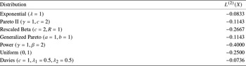
The theoretical values of $L^{(2)}(X)$ for the selected distributions are in Table 3, and are considered for the simulation studies in Tables 4–8.

Table 3.

Theoretical values of $L^{(2)}(X)$ for selected distributions.

Table 3 Long description

Two columns list distribution names and their L second values. Exponential with lambda 1 has minus 0.0833. Pareto two with gamma 1 and c 2 has minus 0.1143, and generalized Pareto with a 1 and b 1 also has minus 0.1143. Rescaled Beta with c 2 and R 1 has minus 0.2667. Uniform from 0 to 1 has minus 0.2500. Davies with c 1, lambda one 0.5, and lambda two 0.5 has minus 0.0736.

Table 4.

Simulation results for the adjacent-spacing estimator for the Uniform $(0,1)$ distribution.

Table 4 Long description

Simulation results are listed by sample size n, with columns for Mean, Variance, Bias, and MSE. For n 10, mean is minus 0.275166, variance 0.001391, bias minus 0.025166, and MSE 0.002023. For n 30, mean is minus 0.258220, variance 0.000321, bias minus 0.008220, and MSE 0.000389. For n 50, mean is minus 0.255097, variance 0.000183, bias minus 0.005097, and MSE 0.000209. For n 100, mean is minus 0.252576, variance 0.000100, bias minus 0.002576, and MSE 0.000106. For n 500, mean is minus 0.250541, variance 0.000018, bias minus 0.000541, and MSE 0.000018.

Table 5.

Simulation results for the adjacent-spacing estimator for the Exponential $(\lambda=1)$ distribution.

Table 5 Long description

Simulation results are listed for an adjacent spacing estimator with columns for n, Mean, Variance, Bias, and MSE. For n 10, Mean is -0.642145, Variance 0.044122, Bias -0.558811, and MSE 0.356348. For n 30, Mean is -0.629870, Variance 0.015506, Bias -0.546537, and MSE 0.314193. For n 50, Mean is -0.619524, Variance 0.008834, Bias -0.536191, and MSE 0.296326. For n 100, Mean is -0.617187, Variance 0.004099, Bias -0.533854, and MSE 0.289095. For n 500, Mean is -0.612111, Variance 0.000851, Bias -0.528778, and MSE 0.280456.

Table 6.

Simulation results for the adjacent-spacing estimator for the Pareto II $(\gamma=1,c=2)$ distribution.

Table 6 Long description

Simulation results are listed by sample size, n, with columns for Mean, Variance, Bias, and MSE. For n 10, mean is minus 0.748809, variance 1.152113, bias minus 0.665475, and MSE 1.593818. For n 30, mean is minus 0.768190, variance 0.510159, bias minus 0.684857, and MSE 0.978678. For n 50, mean is minus 0.717433, variance 0.140208, bias minus 0.634100, and MSE 0.542151. For n 100, mean is minus 0.745770, variance 0.100381, bias minus 0.662437, and MSE 0.539103. For n 500, mean is minus 0.731222, variance 0.018537, bias minus 0.647889, and MSE 0.438279.

Table 7.

Simulation results for the smoothed $k$-spacing estimator $\widehat L_S^{(2)}(X)$.

Table 7 Long description

Simulation results are reported for three distributions, Uniform, Exponential, and Pareto II, with columns for n, Mean, Variance, Bias, and MSE. For Uniform, n values 10, 30, 50, 100, and 500 have means negative 0.262728, negative 0.260406, negative 0.249993, negative 0.249704, and negative 0.250231; variances 0.013830, 0.002443, 0.000911, 0.000380, and 0.000057; biases negative 0.012728, negative 0.010406, 0.000007, 0.000296, and negative 0.000231; and MSE values 0.013989, 0.002551, 0.000911, 0.000380, and 0.000057. For Exponential, the means are negative 0.096857, negative 0.092502, negative 0.087930, negative 0.086605, and negative 0.085102; variances 0.002985, 0.000584, 0.000259, 0.000116, and 0.000019; biases negative 0.013524, negative 0.009169, negative 0.004597, negative 0.003272, and negative 0.001768; and MSE values 0.003168, 0.000668, 0.000280, 0.000127, and 0.000022. For Pareto II, the means are negative 0.132937, negative 0.123069, negative 0.118248, negative 0.116731, and negative 0.115517; variances 0.011896, 0.001520, 0.000804, 0.000338, and 0.000062; biases negative 0.018651, negative 0.008784, negative 0.003962, negative 0.002446, and negative 0.001231; and MSE values 0.012242, 0.001597, 0.000819, 0.000344, and 0.000064. Across all three distributions, variance and MSE decrease as n increases from 10 to 500, while the mean values change more gradually within each distribution.

Table 8.

Simulation results for the regularized $k$-spacing estimator $\widehat L_R^{(2)}(X)$.

Table 8 Long description

Simulation results are reported for three distributions, Uniform, Exponential, and Pareto II, with columns for n, Mean, Variance, Bias, and MSE. For Uniform, Mean is minus 0.256164 at n 10 and minus 0.250176 at n 500; Variance drops from 0.011130 to 0.000057, Bias ranges from minus 0.009010 to 0.000686, and MSE drops from 0.011166 to 0.000057. For Exponential, Mean is minus 0.095668 at n 10 and minus 0.085092 at n 500; Variance drops from 0.002720 to 0.000019, Bias goes from minus 0.012334 to minus 0.001759, and MSE drops from 0.002871 to 0.000022. For Pareto II, Mean is minus 0.129133 at n 10 and minus 0.115496 at n 500; Variance drops from 0.008069 to 0.000062, Bias goes from minus 0.014848 to minus 0.001210, and MSE drops from 0.008287 to 0.000064. At n 100, Variance is 0.000378 for Uniform, 0.000116 for Exponential, and 0.000337 for Pareto II, with corresponding MSE values 0.000378, 0.000126, and 0.000342. Values are listed for n 10, 30, 50, 100, and 500 for each distribution.

To examine the behavior of the estimators, Monte Carlo simulations are performed for different sample sizes. For each distribution and each sample size, $B$ independent random samples are generated. If $\widehat L_b^{(2)}$ denotes the estimate obtained from the $b$th replication, the empirical mean, variance, bias, and mean squared error (MSE) are calculated as

(35)\begin{equation} \operatorname{Mean} = \frac{1}{B} \sum_{b=1}^{B}\widehat L_b^{(2)}, \end{equation}

(36)\begin{equation} \operatorname{Variance} = \frac{1}{B-1} \sum_{b=1}^{B} \left( \widehat L_b^{(2)} -\overline{\widehat L}^{(2)} \right)^2, \end{equation}

(37)\begin{equation} \operatorname{Bias} = \frac{1}{B} \sum_{b=1}^{B}\widehat L_b^{(2)} - L^{(2)}(X), \end{equation}

(38)\begin{equation} \operatorname{MSE} = \frac{1}{B} \sum_{b=1}^{B} \left( \widehat L_b^{(2)}-L^{(2)}(X) \right)^2. \end{equation}

We first examine the behavior of the ordinary adjacent-spacing estimator in (27). The results for the Uniform, Exponential, and Pareto II distributions are presented below.

The results reveal an important limitation of the estimator based on individual spacings. For the Uniform distribution, both the bias and MSE decrease as $n$ increases. In contrast, substantial bias persists for the Exponential and Pareto II distributions even for relatively large sample sizes. This behavior is mainly caused by the reciprocal of individual order-statistic spacings, since a small spacing can make a disproportionately large contribution to the estimator. This observation motivates the use of the smoothed estimator $\widehat L_S^{(2)}(X)$ and the regularized estimator $\widehat L_R^{(2)}(X)$. To assess their finite-sample performance, the simulation experiment is repeated for $ n=10, 30, 50, 100, \text{and }500,$ using $ k=\lfloor\sqrt n\rfloor\ \text{and}\ \epsilon_n=\frac{0.1}{n}. $

For each distribution and sample size, $B=5000$ independent Monte Carlo samples are generated. The empirical mean, variance, bias, and MSE of $\ \widehat L_S^{(2)}(X)$ and $\ \widehat L_R^{(2)}(X)$ are computed in the same manner as above.

The simulation results demonstrate that the smoothed and regularized $k$-spacing estimators substantially improve the finite-sample performance of the adjacent-spacing estimator. In general, the bias, variance, and MSE decrease as the sample size increases, with particularly notable improvements for the Exponential and Pareto II distributions. The smoothed and regularized estimators yield similar results for moderate and large sample sizes, while regularization provides additional stability for smaller samples.

Overall, the results support the use of the $k$-spacing estimators for reliable estimation of quantile-based weighted extropy. These estimators are subsequently applied to the real lifetime datasets in Section 6, using the same choices of $k$ and $\epsilon_n$.

6. Real data applications

In this section, we illustrate the practical applicability of the proposed quantile-based weighted extropy using three real lifetime datasets arising in reliability studies. The analysis is carried out using the nonparametric estimators introduced in Section 5.

Throughout this section, we take $\alpha=2$. First, we compute the adjacent-spacing estimator

(39)\begin{equation} \widehat{L}^{(2)}(X) = -\frac{1}{2n} \sum_{j=1}^{n} u_j \left[ n\left(X_{(j)}-X_{(j-1)}\right) \right]^{-1}, \end{equation}

where

\begin{equation*} u_j=\frac{j-0.5}{n}. \end{equation*}

Since the simulation study indicates that the estimator based on individual spacings may be sensitive to very small spacings, we also use the smoothed $k$-spacing estimator

(40)\begin{equation} \widehat{L}^{(2)}_S(X) = -\frac{1}{2(n-k)} \sum_{j=1}^{n-k} u_j \left[ \frac{n}{k} \left(X_{(j+k)}-X_{(j)}\right) \right]^{-1}, \end{equation}

where $k=\lfloor\sqrt{n}\rfloor$.

For completeness, the regularized estimator

(41)\begin{equation} \widehat{L}^{(2)}_{R}(X) = -\frac{1}{2(n-k)} \sum_{j=1}^{n-k} u_j \left[ \frac{n}{k} \left(X_{(j+k)}-X_{(j)}\right) +\epsilon_n \right]^{-1} \end{equation}

is also considered, with $\epsilon_n=0.1/n$.

6.1. Dataset 1: Failure times of electric carts

The first dataset consists of the times to first failure, measured in months, for 20 small electric carts. These data were originally reported by Zimmer et al. [Reference Zimmer, Keats and Wang43] and subsequently analyzed by Krishnan et al. [Reference Krishnan, Sunoj and Sankaran25]. The observations are

\begin{equation*} \begin{array}{rrrrrrrrrr} 0.9&1.5&2.3&3.2&3.9&5.0&6.2&7.5&8.3&10.4\\ 11.1&12.6&15.0&16.3&19.3&22.6&24.8&31.5&38.1&53.0. \end{array} \end{equation*}

For this dataset, $n=20$ and hence $k=\lfloor\sqrt{20}\rfloor=4$. Application of the three estimators gives

\begin{equation*} \widehat L^{(2)}(X)=-0.006865, \end{equation*}

\begin{equation*} \widehat L_S^{(2)}(X)=-0.004888, \qquad \widehat L_{R}^{(2)}(X)=-0.004888. \end{equation*}

The value obtained from the adjacent-spacing estimator agrees with the value reported earlier in the manuscript. The smoothed estimate is slightly smaller in magnitude, reflecting the reduction in the influence of unusually small individual spacings. Moreover, the smoothed and regularized estimates are almost identical, indicating that the $k$-spacing procedure itself provides adequate numerical stability for these data.

6.2. Dataset 2: Bearing cage failure times

The second dataset consists of failure times, measured in millions of revolutions, of 23 bearing cages from a high-speed textile machine. These data were reported by Lieblein and Zelen [Reference Lieblein and Zelen27]:

\begin{equation*} \begin{array}{rrrrrrrr} 0.14&0.22&0.24&0.27&0.32&0.33&0.35&0.37\\ 0.38&0.42&0.45&0.47&0.49&0.52&0.54&0.58\\ 0.62&0.67&0.73&0.81&0.89&1.01&1.23& \end{array} \end{equation*}

Here $n=23$, so that $k=\lfloor\sqrt{23}\rfloor=4$. We obtain

\begin{equation*} \widehat L^{(2)}(X)=-0.314632, \end{equation*}

while the smoothed and regularized estimates are

\begin{equation*} \widehat L_S^{(2)}(X)=-0.243395, \qquad \widehat L_{R}^{(2)}(X)=-0.241840. \end{equation*}

The difference between the adjacent-spacing and smoothed estimates is more pronounced for this dataset. This may be attributed to the presence of several relatively small spacings among the ordered failure times. Since the estimator involves reciprocals of spacings, such observations can have a substantial effect on the unsmoothed estimate. The $k$-spacing estimator reduces this sensitivity by combining information from several consecutive order statistics.

Again, the regularized estimate is close to the smoothed estimate, suggesting that the $k$-spacing approximation provides sufficient stabilization for the present dataset.

6.3. Dataset 3: Failure times of electrical cables

The third dataset consists of the failure times, measured in hours, of 50 electrical cables under accelerated voltage stress originally reported by Meeker and Escobar [Reference Meeker and Escobar29]. The observations are

\begin{equation*} \begin{array}{rrrrrrrrrr} 1.1&1.9&2.2&2.5&2.8&3.2&3.5&4.0&4.3&5.0\\ 5.2&5.7&6.1&6.5&7.0&7.6&8.2&8.8&9.5&10.3\\ 11.0&11.8&12.6&13.5&14.3&15.2&16.1&17.0&18.0&19.2\\ 20.5&21.8&23.1&24.5&26.0&27.6&29.3&31.0&32.8&34.7\\ 36.7&38.8&41.0&43.3&45.7&48.2&50.8&53.5&56.3&59.2. \end{array} \end{equation*}

For this dataset, 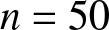$n=50$ and $k=\lfloor\sqrt{50}\rfloor=7$. The estimates are

\begin{equation*} \widehat L^{(2)}(X)=-0.004509, \end{equation*}

\begin{equation*} \widehat L_S^{(2)}(X)=-0.003703, \qquad \widehat L_{R}^{(2)}(X)=-0.003702. \end{equation*}

As in the electric-cart example, the smoothed and regularized estimators are nearly identical. The adjacent-spacing estimator is somewhat larger in magnitude, which is consistent with the sensitivity of the reciprocal-spacing estimator to local variation in consecutive failure times.

6.4. Comparison of the empirical estimates

For convenience, the estimates obtained from the three datasets are summarized in Table 9. The real-data analyses demonstrate the practical applicability of the proposed quantile-based weighted extropy. The estimator based on individual adjacent spacings is more sensitive to local variations, whereas the $k$-spacing estimator provides smoother and more stable estimates by combining consecutive spacings. The small differences between $\widehat L_S^{(2)}$ and $\widehat L_R^{(2)}$ further indicate that regularization has only a minor effect once smoothing is applied. Moreover, these estimators are straightforward to implement using observed order statistics without assuming a specific parametric distribution. The weighting scheme $u^{\alpha-1}$ provides additional flexibility over classical unweighted extropy, making the proposed approach a useful nonparametric tool for uncertainty quantification in lifetime and reliability analysis.

Table 9.

Estimated quantile-based weighted extropy for the three reliability datasets ( $\alpha=2$).

Table 9 Long description

Quantile based weighted extropy estimates are listed for three datasets, alongside n, k, and three estimated measures labeled L hat squared, L hat S squared, and L hat R squared. Electric carts reports n 20 and k 4, with values minus 0.006865, minus 0.004888, and minus 0.004888. Bearing cages reports n 23 and k 4, with values minus 0.314632, minus 0.243395, and minus 0.241840. Electrical cables reports n 50 and k 7, with values minus 0.004509, minus 0.003703, and minus 0.003702. For each dataset, the L hat squared value is more negative than the corresponding L hat S squared and L hat R squared values. L hat S squared and L hat R squared are identical for Electric carts and differ slightly for Bearing cages and Electrical cables.