2. Governing equations

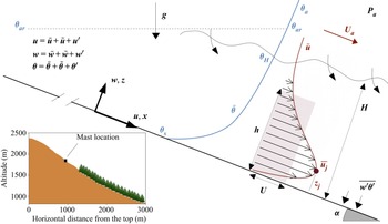
Figure 1 shows a definition sketch of a katabatic flow down a slope of angle $\alpha$, with the inset showing the ground slope topography. The coordinates $(x,z)$ are respectively in the flow directions of streamwise velocity $u(x,z)$ and slope-normal velocity $w(x,z)$. The dry potential air temperature $\theta$ is $\theta _s$ at the ground surface and $\theta _H$ at the outer edge of the jet. The wind speed at a given location $(x, z)$ is in general a function of time depending on the importance of the radiative ground cooling ($\tau$), which varies with the time of day and meteorological conditions. During the evening transition, radiative cooling is generally dominant but then slows down at night, so that a quasi-equilibrium of the heat fluxes is reached. At this state, in the present experiment, $\tau < 1 ^{\circ }$ h$^{-1}$, so that the flow can be assumed to be quasi-steady, i.e. $\tau \ll \mathcal {T}$, where $\mathcal {T}$ represents temperature change on $x$ during the convective time scale $L/\mathcal {U}$, where $\mathcal {U}$ is a characteristic velocity of the wind and $L$ is the slope length.

Figure 1.

Definition sketch of a katabatic wind over a slope of angle $\alpha$. Here, $\overline {u_j}$ and $z_j$ are the maximum wind velocity and the height at which $\bar {u} = \overline {u_j}$, $U_a$ is the ambient wind, $H$ is the height at which the mean velocity $\bar {u}$ equals $5\,\%$ of $\overline {u_j}-U_a$, $\theta _a$ is the ambient temperature profile, $\theta _s$ is the surface temperature, $\theta _{ar}$ is an upstream reference temperature, $\theta _H$ is the ambient temperature at the height $H$, and $P_a$ is atmospheric pressure. The shaded rectangle of dimensions $h$ and $U$ has a flow rate equivalent to the flow rate of the katabatic jet. In the inset, the slope topography is indicated.

Often, an ambient wind of non-negligible speed $U_a$ exists that strongly affects the flow and has to be included in the analysis. In this study we will take into account only its $x$ component parallel to the slope. Transverse ambient winds could affect the flow development, but at present there is insufficient information for evaluating this possible effect.

In the following, $\overline {(\cdot )}$ represents temporal averaging and $(\ )'$ is used for fluctuations around the average value following Reynolds decomposition. Also, $\widetilde{(\ )}$ refers to mean flow oscillations related to ambient stratification $N$, at a frequency close to $N\sin {\alpha }$ (e.g. McNider Reference McNider1982). Applying the boundary layer approximation (see Pope Reference Pope2000, for instance) and decomposing the flow parameters into a mean and fluctuating component, the two-dimensional (2-D) momentum, continuity and heat transfer equations are

(2.1a)$$\begin{gather} (\bar{u}+U_a)\,\frac{\partial (\bar{u}+U_a)}{\partial x} +\bar{w}\,\frac{\partial (\bar{u}+U_a)}{\partial z} + {{\frac{\partial \overline{\overset{{\sim}}{u} ^2}}{\partial x}}} + {{\frac{\partial \overline{u'^2}}{\partial x}}} + \frac{\partial \overline{u'w'}}{\partial z}\nonumber\\ \hspace{-5pc}={-}\frac{1}{\rho_0}\,\frac{\partial (\bar{p} + \overset{{\sim}}{p})}{\partial x} - g\, \frac{\bar{\theta}-\theta_a}{\theta_a}\sin \alpha , \end{gather}$$

(2.1b)$$\begin{gather}\frac{\partial \overline{\overset{{\sim}}{w} ^2}}{\partial z} + \frac{\partial \overline{u'w'}}{\partial x} + \frac{\partial\overline{w'^2}}{\partial z} ={-}\frac{1}{\rho_0}\,\frac{\partial (\bar{p} + \overset{{\sim}}{p})}{\partial z} + g\,\frac{\bar{\theta} -\theta_a}{\theta_a}\cos \alpha , \end{gather}$$

(2.1c)$$\begin{gather}\frac{\partial(\bar{u}+U_a)}{\partial x} + \frac{\partial \bar{w}} {\partial z} = 0 , \end{gather}$$

(2.1d)$$\begin{gather}(\bar{u} + U_a)\,\frac{\partial (\bar{\theta}-\theta_a)}{\partial x} + \bar{w}\,\frac{\partial (\bar{\theta}-\theta_a)}{\partial z} + \frac{\partial \overset{{\sim}}{u}\overset{{\sim}}{\theta}}{\partial x}+\frac{\partial \overline{u'\theta'}}{\partial x} + \frac{\partial \overline{w'\theta'}}{\partial z}\nonumber\\ \hspace{-6pc}= (\bar{u} + U_a) \gamma_{\theta}\sin \alpha +\bar{w}\gamma_{\theta} \cos \alpha , \end{gather}$$

where the viscous terms have been neglected (high Reynolds number and fully rough aerodynamic surface roughness), as well as radiative divergence (Hoch et al. Reference Hoch, Calanca, Philipona and Ohmura2007) and phase change terms. Due to ambient stratification $N^2=g \gamma _{\theta }/\theta _{ar}$ (Stull Reference Stull1988), where $\gamma _{\theta }$ is the temperature gradient and $\theta _{ar} = \theta _{H}(x=0)$ is an upstream reference temperature, the ambient potential temperature $\theta _a$ varies with $x$ and $z$ as (Manins & Sawford Reference Manins and Sawford1979)

(2.2)\begin{gather} \theta_a(z) = \theta_H -\gamma_{\theta}(H-z) \cos\alpha, \end{gather}

(2.3)\begin{gather} \theta_H=\theta_a(z=H) = \theta_{ar} \left(1- \frac{ N^2 x}{g} \left[\sin{\alpha} -\frac{H}{x}\cos\alpha \right]\right), \end{gather}

where $H$ is the height at which the mean velocity is close to zero or $U_a$. By integrating (2.1b) along $z$, then taking the derivative of the resulting expression along $x$, we obtain an expression for the pressure variation along $x$ in (2.1a) (the form can be found in Haiden & Whiteman Reference Haiden and Whiteman2005, for example). Then, after neglecting the mean flow oscillation $\overset {{\sim} }{u}^2 \ll \bar {u}^2$ (§ 4) as well as the $x$ variations of turbulent quantities, $\overline {u'^2}$ and $\overline {w'^2}\ll \bar {u}^2$ and $\overline {u'\theta '}\ll \bar {u} \bar {\theta }$, and taking $U_a$ constant, the system of equations becomes

(2.4a)$$\begin{gather} \frac{\partial (\bar{u} +U_a)\bar{u}}{\partial x} + \frac{\partial \bar{u} \ \bar{w}}{\partial z} + \frac{\partial \overline{u'w'}}{\partial z} ={-} g\,\frac{\bar{\theta}-\theta_H}{\theta_a}\sin \alpha + g \cos \alpha\,\frac{\partial}{\partial x}\int_z^H\left(\frac{\bar{\theta}-\theta_a}{\theta_a}\right) {\rm d}z' , \end{gather}$$

(2.4b)$$\begin{gather}\frac{\partial (\bar{\theta}-\theta_a)(\bar{u}+U_a)}{\partial x} + \frac{\partial (\bar{\theta}-\theta_a)\bar{w}}{\partial z} ={-}\frac{\partial \overline{w'\theta'}}{\partial z} +(\bar{u} + U_a)\gamma_{\theta} \sin \alpha +\bar{w} \gamma_{\theta}\cos \alpha . \end{gather}$$

Because the variation of $\theta _a$ is negligible over the height $H$ with respect to the variation of the temperature profile, we can take $\theta _a = \theta _H$ in the terms on the right-hand side of (2.4a). Then, under the assumption of velocity and temperature profiles similarity, integration of (2.4) along $z$ results in equations for the integral mean velocity $U$ and temperature variation $\Delta \varTheta$. At $z=H$, we consider that turbulent fluxes tend to 0. The steady-state depth-integrated equations obtained are similar to those of Manins & Sawford (Reference Manins and Sawford1979) with ambient velocity added:

(2.5a)$$\begin{gather} \frac{{{\rm d}(U+U_a)U}{h}}{{\rm d}\kern0.7pt x} = g\,\frac{S_2\,\Delta\varTheta}{\theta_H}\,h\sin{\alpha}-\frac{1}{2}g\,\frac{{\rm d}}{{\rm d}\kern0.7pt x}\left(\frac{S_1\, \Delta\varTheta}{\theta_H}\,h^2\cos{\alpha}\right)-C_D\left(U+\frac{U_a}{2}\right)^2 , \end{gather}$$

(2.5b)$$\begin{gather}\frac{{\rm d}(U+U_a)\,\Delta\varTheta\,h}{{\rm d}\kern0.7pt x} ={-}\overline{(w'\theta')}_s -(U+U_a)h\gamma_{\theta} \sin{\alpha} . \end{gather}$$

The last term in (2.4b) has been neglected, because $(H/x)\cos \alpha \ll \sin \alpha$ ($H{\sim} 0.03x)$. Here, $C_D=-\overline {(u'w')_s}/(U+U_a/2)^2$ is the bottom drag coefficient, where changes of $C_D$ due to the mean flow oscillations are averaged out over the katabatic event considered. We chose to use $U_a/2$ so that when $U=-U_a$, the bottom drag is not zero. The turbulent sensible heat flux $\overline {(w'\theta ')_s}$ is negative. The integral quantities $U$, $h$, $\Delta \varTheta$ and the profile shape factors $S_1$, $S_2$ (which are considered constants) are defined by

(2.6a,b)\begin{gather} Uh = \int_0^H \bar{u}\,{\rm d}z, \quad U^2h = \int_0^H\bar{u}^2\,{\rm d}z , \end{gather}

(2.7a,b)\begin{gather} S_2\,{\Delta \varTheta}\,h ={-}\int_{0}^H \left(\bar{\theta}-\theta_a\right) {\rm d}z, \quad S_1\, {\Delta \varTheta}\,h^2 ={-}2\int_{0}^H \left(\bar{\theta}-\theta_a\right) z \,{\rm d}z . \end{gather}

The integrated buoyancy flux $B$ is defined by

(2.8)\begin{align} B= \frac{g{(U+U_a)}\,{\Delta \varTheta}\,h}{\theta_H} =K\,\frac{g{(U+U_a)} {(\theta_{H} - \theta_s}) h}{\theta_H}={-}\frac{g}{\theta_{H}}\int_{0}^H (\bar{\theta}-\theta_{a})(\bar{u}+U_a) \,{\rm d}z, \end{align}

where $K= \Delta \varTheta /(\theta _H-\theta _s)$. The coefficients $S_1$, $S_2$ and $K$ are obtained by integrating over $z$ the measured velocity and temperature profiles. The integrated buoyancy (2.8) is also obtained by integrating (2.5b) by taking variations of the parameters in the form $\overline {(w'\theta ')}_s {\sim} x^m$, $U{\sim} x^n$ and $E_h = {\rm d}h/{{\rm d}\kern0.7pt x}$. This gives

(2.9)\begin{align} B=\frac{g(U+U_a)\,\Delta\varTheta\,h}{\theta_H} ={-}\frac{g}{\theta_H}\,\frac{\overline{(w'\theta')}_s}{m+1}\,x \left(1+ \frac{h \gamma_{\theta} \sin \alpha (m+1)}{\overline{(w'\theta')}_s} \left[ \frac{U}{n+2} + \frac{U_a}{2}\right] \right) . \end{align}

With the parameters $U$, $h$, $\Delta \varTheta$ and $B$, we can define the global Richardson number $Ri_0$ (see (2.10)) and the entrainment coefficient $E$ (see (2.11)) as

(2.10)\begin{gather} Ri_0=g\,\frac{\Delta \varTheta\,h}{\theta_H U^2}\cos{\alpha} =\frac{B}{U^2(U+U_a)}\cos\alpha , \end{gather}

(2.11)\begin{gather} E=\frac{1}{U}\,\frac{{\rm d}(U+U_a)h}{{\rm d}\kern0.7pt x} = \left(1+\frac{U_a}{U}\right)E_h + E_U, \end{gather}

where $E_h$ and $E_U = (h/U) \,{\rm d}(U+U_a)/{{\rm d}\kern0.7pt x}$ relate to the spatial variation of volume flux due to the increase of current height and to the change of mean velocity, respectively. By virtue of the entrainment assumption (Morton, Taylor & Turner Reference Morton, Taylor and Turner1956), $E$, which is a function of $Ri_0$ (Turner Reference Turner1973), can be considered constant along $x$ because $Ri_0$ remains constant when the ambient velocity $U_a=0$. The current height grows linearly with $x$ ($E_h$ constant) so that $E_U$ is also constant. When $U_a\ne 0$, the growth of current height is slowly varying with $x$: ${\rm d}h/{{\rm d}\kern0.7pt x}=(E-E_U)/(1+U_a/U)$. It is also possible that $E$, in addition to $Ri_0$, is a function of $U_a$. The analysis of the present measurements (§ 4) seems to indicate a dependency on $U_a$. Finally, after rearrangement of (2.5a) and using the above-defined parameters $Ri_0$, $E$ and $E_U$, we get the integral velocity in terms of integrated buoyancy flux in the form

(2.12)\begin{align} \frac{U^3}{B} = \frac{S_2 \sin \alpha - \dfrac{S_1 h}{2 B} \cos \alpha\,S_1\,\dfrac{{\rm d}B}{{\rm d}\kern0.7pt x}}{E \left[\left(1+\dfrac{U_a}{U}\right)+\dfrac{1}{2} S_1\,Ri_0\right] + E_U \left[\left(1+\dfrac{U_a}{U}\right)^2 - S_1\,Ri_0\right]+ C_D \left(1+\dfrac{U_a}{2U}\right)^2 \left(1+\dfrac{U_a}{U}\right)} . \end{align}

Equation (2.12) shows the force balance involved, with the integrated buoyancy flux $B$ driving the flow, and entrainment $E$ plus $E_U$ and bottom friction, expressed by $C_D$, retarding the flow.

When the heat flux to the ground $\overline {(w'\theta ')}_s$ is assumed to be constant along $x$ and ambient stratification is negligible, (2.5b) leads to $U\,\Delta \varTheta \,h = - \overline {(w'\theta ')}_sx$, which corresponds to (2.24) of Manins & Sawford (Reference Manins and Sawford1979). When making use of the entrainment assumption $E_h ={\rm d}h/{{\rm d}\kern0.7pt x} = \text {const.}$, such that $h{\sim} x$, and when $U_a = 0$, we have $U\,\Delta \varTheta {\sim} x^{0}$ and $U^2 {\sim} \Delta \varTheta \,h$, hence $U {\sim} x^{1/3}$ and $\Delta \varTheta {\sim} x^{-1/3}$ (Appendix A). Manins & Sawford (Reference Manins and Sawford1979) and Ellison & Turner (Reference Ellison and Turner1959) assumed the heat flux to be constant along the slope, which seems to be a satisfactory approximation as was seen from the comparison of measured and calculated velocities in Manins & Sawford (Reference Manins and Sawford1979). However, as shown by (2.5b), ambient stratification causes a decrease in the integrated buoyancy flux $B$ even for constant heat flux $\overline {(w'\theta ')}_s$ so that a $1/3$ power law can be an approximation only over a limited slope length depending on stratification $N$ and the slope angle $\alpha$. Furthermore, ambient wind also modifies the $1/3$ power law and causes a deviation of $h$ from a linear growth (2.11). For a uniform ambient temperature, i.e. $N=0$, such that $\Delta \varTheta \approx \text {const.}$ (negligible variations of surface temperature), and no ambient wind $U_a$, (2.5a) and (2.5b) impose $U{\sim} x^{1/2}$, with the heat flux to the ground increasing as ${\sim} x^{1/2}$ (Appendix A). These power laws will be discussed further in § 4, where the theory is used in the analysis of the present experimental data sets.

3. Instrumentation and field measurement conditions

Two experimental data sets have been obtained during field experiments in November 2012 (Blein Reference Blein2016; Charrondière et al. Reference Charrondière, Brun, Sicart, Cohard, Biron and Blein2020) and February 2019 (Charrondière et al. Reference Charrondière, Brun, Cohard, Sicart, Obligado, Biron, Coulaud and Guyard2022), in the Belledonne mountain range (near Grenoble, France), under cloud-free anticyclonic conditions, which are the best conditions in which to observe katabatic flows.

The 2012 data were obtained with a 6 m high mast positioned on a ground slope of approximately $30^{\circ }$ (estimated from a digital elevation model with horizontal resolution 25 m) at distance $L\approx 1100$ m from the top. The ground was covered by sparse small bushes and rocks, and hence was very rough, of drag coefficient $C_D \approx 0.04$ as defined in table 1. The mast has been equipped with: three three-dimensional (3-D) sonic anemometers of sampling frequency $f=20$ Hz (Campbell Scientific, CSAT3), positioned at slope-normal heights $z=0.93$ m, $1.65$ m and $3.70$ m; one 3-D sonic anemometer of frequency $f=10$ Hz (WindMaster Pro from Gill Instruments) positioned at $z=5.88$ m; a thermo-hygrometer (CS215, Campbell Scientific) of frequency $f=0.5$ Hz at $z=1.48$ m; a 2-D sonic anemometer (WindSonic, Gill Instruments) of frequency $f=0.5$ Hz at $z=2.87$ m; and an infrared thermometer to estimate surface temperature (KT15, Heitronics) of frequency $f=0.5$ Hz. In the present study, we focus on a katabatic event of practically no ambient wind. It lasted 30 min from 19:15 to 19:45 local time (LT = UTC + 1) on 19 November 2012. The data set has been processed following Charrondière et al. (Reference Charrondière, Brun, Sicart, Cohard, Biron and Blein2020), using a Reynolds decomposition at a time scale of 2 min, resulting in 15 segments during the katabatic event.

Table 1.

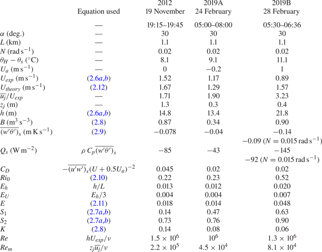
Experimental and calculated parameters of the katabatic wind for the three considered events 2012, 2019A and 2019B (§ 2). The entrainment coefficient $E$ has been calculated from (2.11) using experimental values of $E_h$. The turbulent sensible heat fluxes close to the surface have been determined with ambient stratification $N=0.02$ rad s$^{-1}$ and, for comparison, with $N=0.015$ rad s$^{-1}$ in 2019B.

The 2019 data set was obtained with a 10 m high mast, also positioned over a slope of approximately $30^{\circ }$, at a downstream distance $L\approx 1100$ m, close to the position of the 2012 set-up. The ground was covered with snow that reduced the surface roughness, $C_D \approx 0.02$ (§ 4). The measurements were conducted from 12 to 28 February 2019, also under anticyclonic conditions. The katabatic wind velocities were measured with seven 3-D sonic anemometers of frequency $f=20$ Hz positioned at slope-normal heights $z=0.31$ m (Campbell Scientific, CSAT3B), 0.66 m, 0.98 m, 1.5 m, 1.93 m, 2.37 m (Campbell Scientific, CSAT3) and 9.77 m (Gill Instruments, WindMasterPro). The highest sonic anemometer provided a large temperature bias in both the 2012 and the 2019 data sets even after sonic temperature correction. For this reason, we chose not to use them in the present paper. Furthermore, four 2-D sonic anemometers ($f=0.5$ Hz), positioned at $z= 3.14$ m, 4.19 m, 6.02 m and 7.71 m (WindSonics, Gill Instruments), were used. Temperatures were measured with 10 thermocouples ($f=20$ Hz) located at $z= 0.33$ m, 0.41 m, 0.49 m, 0.58 m, 0.68 m, 0.77 m, 2.95 m, 4 m, 5.84 m and 7.52 m (Campbell Scientific). These heights are with respect to the snow cover on 24 February, which is the first night used in the present study. These heights changed by approximately 13 cm with changing snow cover depth from this night until the end of the experiments. Surface temperature was determined from pyrgeometer measurements (CG3 from Kipp & Zonen) at 10 min intervals. The data were processed following Charrondière et al. (Reference Charrondière, Brun, Cohard, Sicart, Obligado, Biron, Coulaud and Guyard2022), using a Reynolds decomposition at a time scale of 2 min. From the 2019 data set, we chose for the present analysis two katabatic events respectively with weak and strong ambient winds. These two events are:

1. (i) 2019A: measurements from 05:00 to 08:00 LT on 24 February (‘6d’ event in Charrondière et al. Reference Charrondière, Brun, Cohard, Sicart, Obligado, Biron, Coulaud and Guyard2022);

2. (ii) 2019B: measurements from 05:30 to 06:36 LT on 28 February (‘7’ event in Charrondière et al. Reference Charrondière, Brun, Cohard, Sicart, Obligado, Biron, Coulaud and Guyard2022).

In order to complement the data in the boundary region of the wind, a 3-D multi-hole Pitot probe (Cobra probe, Turbulent Flow Instrumentation Pty Ltd, Australia) has been used from 3 cm to 28 cm height above the snow surface, at sampling frequency 1250 Hz. Six 1 min time series of 3-D velocity components were acquired between 05:55 and 06:36 LT during the 2019B event and processed in the streamline coordinate system (Charrondière et al. Reference Charrondière, Brun, Cohard, Sicart, Obligado, Biron, Coulaud and Guyard2022). A tethered balloon was used in a clearing lower in altitude to provide ambient stratification. This balloon is equipped, among others things, with a thermo-hygrometer (see Charrondière et al. Reference Charrondière, Brun, Cohard, Sicart, Obligado, Biron, Coulaud and Guyard2022, for more details).

4. Mean flow development and comparison with theory

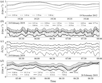
It is well known that the mean flow of katabatic winds oscillates at a frequency close to $N\sin {\alpha }$. Fleagle (Reference Fleagle1950), McNider (Reference McNider1982) and Helmis & Papadopoulos (Reference Helmis and Papadopoulos1996), for instance, developed a compressional warming model to explain these oscillations, whereas Princevac et al. (Reference Princevac, Hunt and Fernando2008) suggested an internal wave mechanism. Figure 2 shows the temporal variation of the mean wind velocity of the three katabatic events, and of the temperature for one of them (averaged on 2 min based on a multi-resolution decomposition as shown in Charrondière et al. Reference Charrondière, Brun, Cohard, Sicart, Obligado, Biron, Coulaud and Guyard2022). The temperature variations are included in order to show that these are largest near the ground and are out of phase with respect to the velocity variations, i.e. increasing velocity is related to decreasing temperature, and vice versa. The amplitude of the velocity oscillations is sufficiently low ($<0.4$ m s$^{-1}$) so that the term $\partial \overset {{\sim} }{u} ^2/\partial x$ is approximately $10^{-4}$ m s$^{-2}$, and $\overset {{\sim} }{u}^2/\bar {u}^2 {\sim} 4.10^{-2}\ll 1$ and can therefore be neglected in the depth-integrated model of mean velocities developed in § 2.

Figure 2.

Along-slope mean wind variations of the three katabatic events defined in § 3: (a) 2012, (b) 2019A, and (d) 2019B. (c) Temporal temperature variations of the 2019A katabatic event.

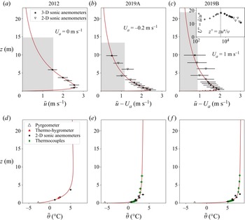
Figure 3 shows the profiles of along-slope wind velocity $\bar {u}-U_a$ and the corresponding temperature profiles $\bar {\theta }$, for the three katabatic events described in § 3. These profiles are ensemble averages, of the 2 min averages, over the length of each katabatic event. The fitted profiles (continuous lines) are obtained by using a fitting procedure that is based on an adaptation of the Prandtl model (Prandtl Reference Prandtl1942), with varying eddy-diffusivity coefficient introduced by Grisogono & Oerlemans (Reference Grisogono and Oerlemans2001). The procedure is discussed in detail in Brun et al. (Reference Brun, Blein and Chollet2017) and Charrondière et al. (Reference Charrondière, Brun, Sicart, Cohard, Biron and Blein2020). A noticeable difference between the 2012 and 2019 velocity profiles is the much higher location of the velocity maximum in the 2012 event. The most plausible explanation is the larger roughness on the snow-free surface causing a higher turbulence level with respect to 2019 measurements. Furthermore, the near ground temperature gradient is less than in the 2019 events obtained on a snow cover.

Figure 3.

(a–c) Along-slope wind velocity profiles, and (d–f) temperature profiles, corresponding to (a,d) the 2012 katabatic event, (b,e) the 2019A katabatic event, and (c, f) the 2019B katabatic event. The filled symbols (resp. the error bars) represent measured mean values (resp. the standard deviations) of the 2 min segments of each event. The continuous lines are fitted profiles of wind speed and temperature according to the Prandtl-based fitting model (Brun et al. Reference Brun, Blein and Chollet2017; Charrondière et al. Reference Charrondière, Brun, Sicart, Cohard, Biron and Blein2020). The shaded areas in (a–c) represent the integral velocity $U$ and integral height $h$, corresponding to the red fitting line. The inset in (c) shows a linear–log plot of the velocity, indicating a log variation of $\bar {u}$ near the velocity maximum (Charrondière et al. Reference Charrondière, Brun, Cohard, Sicart, Obligado, Biron, Coulaud and Guyard2022).

Ambient wind $U_a$ has been determined from the shape of the fitted profiles, and the experimental conditions. In the 2012 katabatic event, which is an ideal katabatic case that lasted only 30 min, ambient wind was close to zero. The 2019A katabatic event was extracted from a relatively calm night of measurements, when ambient wind was low and stable. The shape of the velocity profile suggests a slight up-slope wind of velocity $U_a=-0.2$ m s$^{-1}$ (figure 3b). The 2019B event (figure 3c) corresponds to a night with strong ambient wind. By comparing the velocity profiles shown in figure 3, it is seen that ambient wind $U_a$ has a strong effect on the profile shapes. While in the 2019B event, the katabatic wind velocity profile joins smoothly the relatively strong ambient wind ($U_a{\sim}eq 1$ m s$^{-1}$), the profile in the 2019A event is more concave, with $\overline {u_j}/2$ (where $\overline {u_j}$ is maximum wind velocity) already observed at $3.5$ m height (against 14 m in the 2019B event). The inset in figure 3(c) shows a lin-log plot of velocity, indicating a log variation over more than one decade near maximum velocity. This is typical variation observed in all the 2019 events.

The characteristic parameters of these katabatic events are summarized in table 1. We evaluated $U_{exp}$ and $h$ from (2.6a,b), integrated up to the height where $\bar {u}$ is within $5\,\%$ of $\overline {u_j}-U_a$. Provided that the integrated buoyancy flux $B(x)$ is known, katabatic wind velocity at any downstream location $x$ can be calculated from (2.12) using the values of $E$, $E_U$, $Ri_0$ and $C_D$ given in table 1, with $E$ given by (2.11), using $E_h$ determined from experiments and $E_U {\sim}eq E_h/3$ (under the assumption that $E_h$ is a constant and $U {\sim} x^{1/3}$). When $U_a\ne 0$, it is necessary to evaluate $(1+U_a/U)$. For this, an iterative procedure was used, first calculating the velocity in the absence of $U_a$ to get an evaluation of $U$, and then recalculating with $U_a$ until convergence. From table 1, it is seen that the depth-averaged velocities calculated from (2.12), using the experimental value of $B$ at the location $x=L$, are in good agreement with the measured values, with the largest difference being for the 2019B event, where there exists a strong ambient wind $U_a$. The value of $E$ without ambient wind (2012 event) obtained from the extrapolated profiles lies within the range of $E$ measured in laboratory, constant buoyancy supply, gravity current experiments, where $0.018\lesssim E \lesssim 0.038$ on a slope of $30^{\circ }$ (Turner Reference Turner1973). However, the spread is considerably larger in the presence of ambient wind, which, besides some uncertainty related with the extrapolation, would indicate that $E$ in addition to being a function of $Ri_0$ depends also on $U_a$.

In table 1, $C_D$ has been evaluated from $U_{exp}$ and from the turbulent momentum flux close to the surface $\overline {(u'w')}_s$. The value of $\overline {(u'w')}_s$ has been determined from the model proposed by Denby & Smeets (Reference Denby and Smeets2000), as presented in Charrondière et al. (Reference Charrondière, Brun, Cohard, Sicart, Obligado, Biron, Coulaud and Guyard2022). Contrary to laboratory gravity currents on smooth walls, where $C_D$ is small and negligible compared with $E$ when the slope angle $\alpha >5^{\circ }$ (§ 1), bottom drag cannot be neglected in the katabatic winds analysed here, where the ground surface is very rough in the case of no snow (aerodynamic roughness $z_0\approx {1}$ cm, $C_D\approx {0.04}$) and rough with snow cover ($z_0\approx {0.3}$ mm, $C_D\approx {0.02}$,) so that $C_D$ is of the same order as $E$ even on steep slopes (table 1). The shape parameters $S_1$ and $S_2$ are determined from (2.6a,b) (as in Manins & Sawford Reference Manins and Sawford1979), after $\Delta \varTheta$ and $K$ are determined from (2.8). The shape parameters $S_1$ and $S_2$ for the 2019 events are close to those obtained by Manins & Sawford (Reference Manins and Sawford1979), who determined $S_1=0.5$ and $S_2=0.9$ for their katabatic flow. The lower values in the 2012 event come from the oscillatory behaviour of the temperature profile that we used in the form $\bar {\theta } - \theta _a = \theta _0 \cos (z/l_0) \exp {(-z/l_0)}$, where $\theta _0$ and $l_0$ are temperature and length scales of the flow (Prandtl Reference Prandtl1942). The first height $H_{\theta }$ at which $\bar {\theta } = \theta _a$ is lower than $H$ because the wavelength of this oscillation is shorter than $H$. We thus integrated the temperature profile only up to $H_{\theta }$ when determining $S_1$, $S_2$ and $B$.

In the neutral case ($N = 0$ rad s$^{-1}$), a constant reduced gravity $\Delta \varTheta$ along $x$ means that $U{\sim} x^{1/2}$ and $m=1/2$ (heat flux to the ground increases with $x$, described in § 2 and Appendix A). Such an increase in $U$ would give wind speeds that are considerably larger than the measured values. As mentioned in § 2 (and explained in Appendix A), constant heat flux to the ground gives $U{\sim} x^{1/3}$ and requires that $\Delta \varTheta {\sim} x^{-1/3}$ to first order. Because of the steep slope in the present experiment, ambient stratification results in an appreciable decrease of $\theta _H$ along $x$, hence of $\Delta \varTheta$ with $x$ if $\theta _s=\text {const.}$ as seen from (2.3). Surface potential temperature may adjust to air temperature with time, thus it may also decrease with $x$, because of the stratification combined with a steep slope. This constant surface heat flux solution, consistent with the present observational data, means that the decrease of surface temperature is slower than the decrease of ambient temperature $\theta _H$. A deviation from $\Delta \varTheta {\sim} x^{-1/3}$ implies a non-constant heat flux to the ground. However, the present data indicate that the assumption of constant heat flux is a good approximation over the distance $L\approx 1.1$ km (see figure 4a). The heat flux to the ground $\overline {(w'\theta ')}_s{\sim} x^{m}$, given in table 1, has thus been evaluated from (2.9) with $n=1/3$ and assuming the heat flux to be constant along the slope, i.e. $m=0$. The solution may be slightly different from $U {\sim} x^{1/3}$ due to the steep slope angle (figure 4b) combined with stratification (figure 4c) and ambient wind, and also because the surface sensible heat flux may vary slightly along $x$.

Figure 4.

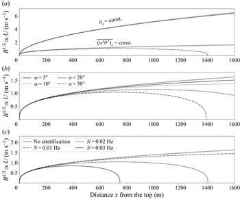
Parametric study of $U{\sim} B^{1/3}$ as a function of $x$. (a) Constant $\Delta \theta$ ($m=1/2$ and $n=1/2$) and constant $\overline {(w'\theta ')_s}$ ($m=0$ and $n=1/3$) with (black lines) and without (grey lines) stratification effects. (b) Effect of slope angle $\alpha$ for constant $\overline {(w'\theta ')_s}$ over $x$. The grey line is the present case of a $30^{\circ }$ slope without stratification. (c) Effect of ambient stratification $N$ for constant $\overline {(w'\theta ')_s}$ over $x$.

With $\overline {(w'\theta ')}_s =\overline {w'\theta '}_{sr}(x/x_0)^m$ and $U =U_r(x/x_0)^n$ (the subscript $r$ stands for reference, taken at $x_0$ m from the beginning of the slope), 2.9 takes the form

(4.1)\begin{align} B={-}\frac{g}{\theta_H}\,\frac{\overline{w'\theta'_{sr}}}{x_0^m}\,\frac{x^{m+1}}{m+1} \left(1+E_h \gamma_{\theta} \sin \alpha\,\frac{x_0^m}{\overline{w'\theta'_{sr}}}\,(m+1) x^{1-m} \left[ \left(\frac{U_r}{x_0^n}\right) \frac{x^n}{n+2} + \frac{U_a}{2}\right]\right) . \end{align}

Taking $x_0=100$ m, the downstream variation of the mean velocity $U{\sim} B^{1/3}$ can be obtained as a function of external parameters. The default values in this equation are the experimental results of the 2012 katabatic event, with $U_a=0$ m s$^{-1}$, $\alpha =30^{\circ }$, $N=0.02$ rad s$^{-1}$, $m=0$ and $n=1/3$. The initialization parameters $\overline {w'\theta '}_{sr}$ and $U_r$ are determined with $m=0$ and are the same in all cases considered. Figure 4(a) provides the downstream variation of $B^{1/3}$ $(U{\sim} B^{1/3})$ for the two above-mentioned possibilities – surface temperature constant or surface heat flux constant. These solutions are computed in the neutral case and in the more realistic case of stably stratified environment. In figure 4(b), the effect of the slope angle is shown for conditions approximating the present events ($n=1/3$, $m=0$). In figure 4(c), the effect of ambient stratification is shown. In the whole, figure 4 shows that $U{\sim} B^{1/3}$ increases with $x$ up to a point where it reaches a maximum value before decreasing. The maximum value of $U$, its position and the position of $U=0$ m s$^{-1}$ vary depending on the set of parameters used in the equation. It seems that the present measurements were taken near the location of maximum velocity or slightly beyond.

The powers $n$, $m$ and $p$ are likely to change along the slope. Using constant values of this set of parameters is valid only for a limited distance $x$. The katabatic flow is probably accelerating on the first part of the slope, before slowing down with distance. According to the above demonstration and simulations by Brun et al. (Reference Brun, Blein and Chollet2017), the wind may slow down and even stop before arriving in the valley. However, it is likely that at lower altitudes, the reference temperature increases so that a temperature difference is maintained.

Between the two katabatic events 2019A and 2019B, the turbulent heat flux $\overline {(w'\theta ')}_s$ varies by a factor of 3, even though the surface conditions (presence of snow, slope and radiative budget of approximately $-65$ W m$^{-2}$) are quite close. The difference between the two events can be attributed partly to the presence of the strong ambient wind $U_a$ in the 2019B event. Furthermore, sublimation of the snow surface is likely to be non-negligible in the 2019B event, because specific humidity of the surface (estimated from surface temperature with the assumption that relative humidity is 100 %) is nearly twice the specific humidity measured at 3.8 m height. In the presence of strong ambient wind, there is also some uncertainty about the value of $N$, and as indicated in table 1, a value $N=0.015$ rad s$^{-1}$ results in a substantially lower heat flux.

5. Turbulent fluxes and mixing efficiency

A better understanding of the relation between turbulent quantities and mean flow behaviour is of interest for parametrizing turbulence fluxes in katabatic wind models. The depth-integrated model gives access to the $x$ development of the integral parameters, notably $U$ and $h$, assuming profile similarity. The turbulent fluxes in the jet, determined in this section, scale on these parameters, hence the importance of knowing the mean flow development. Furthermore, from the mean flow analysis, an estimate of the turbulent sensible heat flux close to the surface $\overline {(w'\theta ')}_s$ is obtained (see (2.9)). In the following, we consider first the outer mixing region $z>z_j$ (§ 5.1) and then the inner layer $z< z_j$ (§ 5.2), where $z_j$ is the height of maximum jet velocity $\overline {u_j}$.

5.1. Outer mixing region

The outer, free shear region is the region above the position $z_j$. Turbulence measurements have been conducted at two heights above $z_j$ in the 2012 event and at five heights in the 2019 field measurements. The two lowest measurement levels in the 2012 event and the lowest level in the 2019 events were too close to the maximum wind velocity to be considered as part of the outer mixing region of the jet.

The slope-normal turbulent fluxes of momentum and heat (density) are respectively given by the Reynolds shear stress $\overline {u'w'}$ and $\overline {w'\theta '}$, from which the corresponding eddy coefficients $K_m$ and $K_h$, and their relation with the mean gradients, hence also the Richardson number, can be determined. 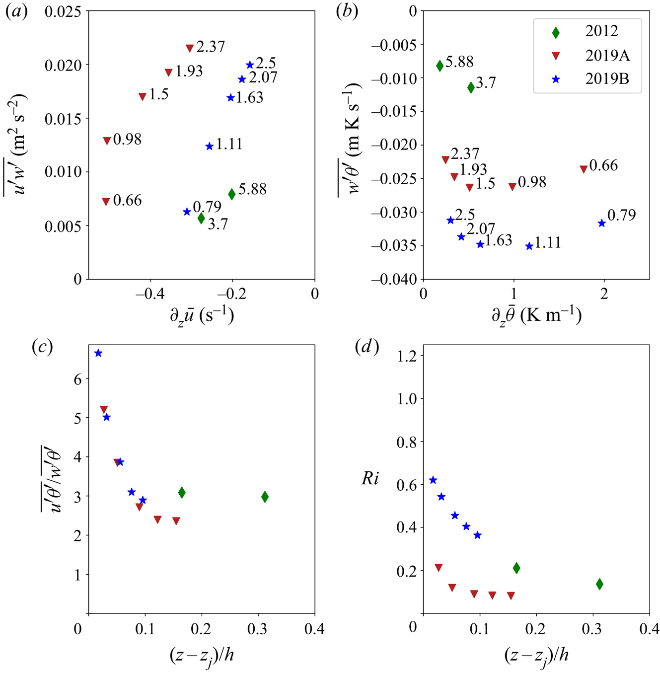The relation between turbulent fluxes and local mean gradients is valid since the equilibration time scale $H/u_*$ is at least an order of magnitude lower than the advection time scale $L/U$, which means that the turbulent fluxes have enough time to equilibrate with the local mean gradients. Figures 5(a) and 5(b) show the turbulent shear stress $\overline {u'w'}$ and slope-normal heat flux $\overline {w'\theta '}$ as functions of their respective gradient, $\partial \bar {u}/\partial z$ and $\partial \bar {\theta }/\partial z$. An interesting observation is the rapid decrease of velocity gradient (similar to a boundary layer) above its maximum value that is located very close to $z_j$. In gravity currents (e.g. Odier et al. Reference Odier, Chen, Rivera and Ecke2009), the maximum of velocity gradient is at nearly half the current height, which differs considerably from the present katabatic wind conditions. The local gradient Richardson number $Ri$, defined in (5.1), is shown in figure 5(d) as (Oldroyd et al. Reference Oldroyd, Pardyjak, Higgins and Parlange2016)

(5.1)\begin{equation} Ri = \frac{g}{\bar{\theta}} \cos \alpha\,\frac{\partial \bar{\theta}}{\partial z}\left(\frac{\partial \bar{u}}{\partial z}\right)^{{-}2} . \end{equation}

Figure 5.

(a) Turbulent flux of momentum as a function of mean velocity gradient for the 2012 and two 2019 katabatic events in the mixing region above the maximum wind speed. (b) Slope-normal component of turbulent heat flux as a function of the mean temperature gradient. The numbers next to the markers are the heights in metres measured from the ground in the slope-normal direction. (c) Ratio of the along-slope to the slope-normal turbulent heat fluxes. (d) Gradient Richardson number $Ri$ determined from slope-normal profiles. The slope-normal height with respect to the maximum wind velocity height $z_j$ is normalized by the integral height $h$ given in table 1.

As expected, $Ri$ decreases with increasing $z/h$. The highest values and variations are located close to the maximum wind velocity, i.e. near $z_j$. Values range from $Ri=1.2$, near but above $z_j$ in the 2019B event, to approximately $Ri=0.11$ at the upper measurement levels in the 2019A event. Odier et al. (Reference Odier, Chen, Rivera and Ecke2009) showed that in the outer mixing region of a laboratory gravity current, eddy coefficients $K_m$ and $K_h$ increase with increasing gradient, whereas the mixing lengths are constant. However, in their case, the gradient Richardson number is small ($Ri\approx 0.08$) and practically constant.

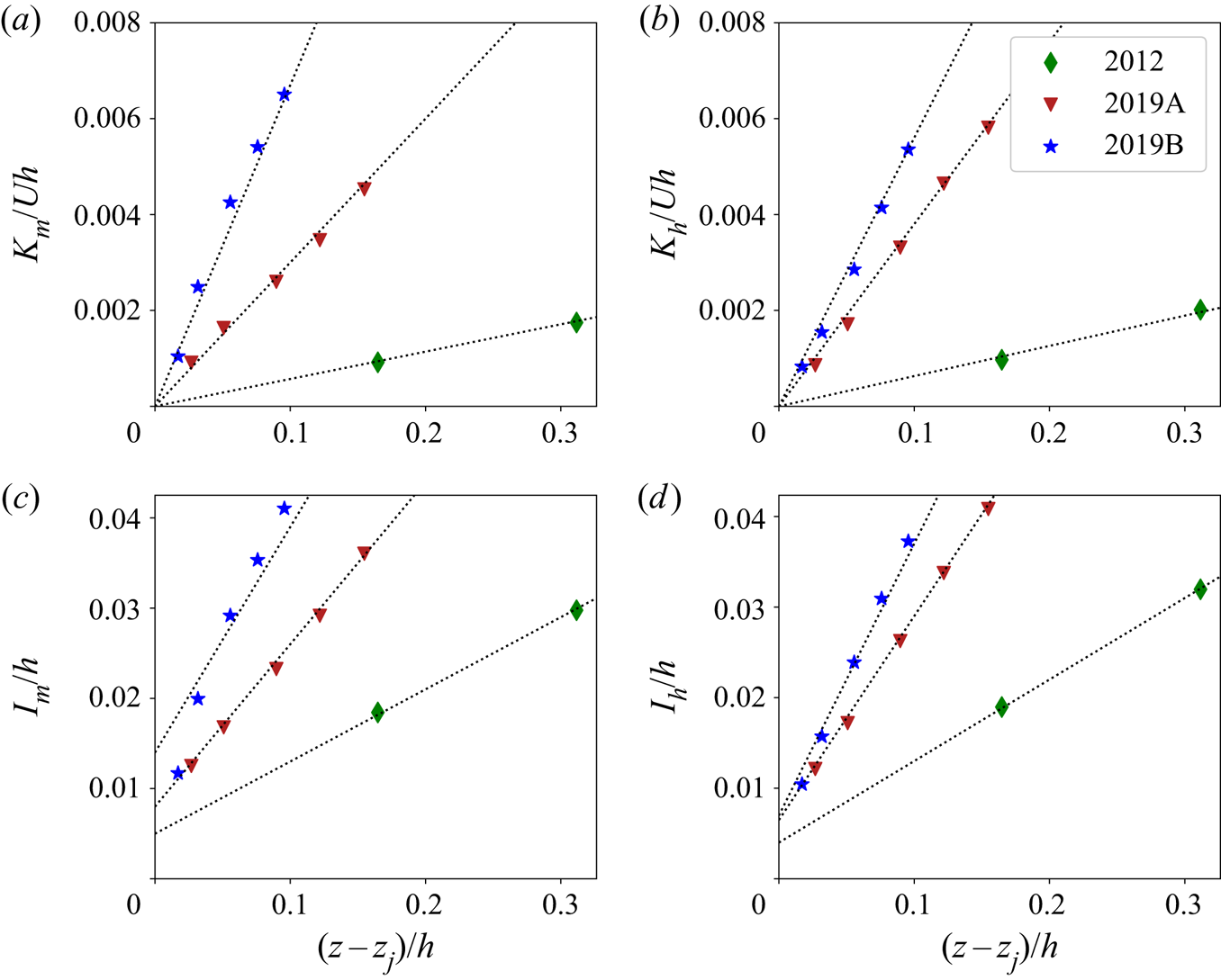
Interestingly, in the present study, the eddy coefficients increase nearly linearly with height (figures 6a,b), with their values being $0.014/Uh\lessapprox K_m/Uh \lessapprox 0.12/Uh$ and $0.013/Uh\lessapprox K_h/Uh \lessapprox 0.1/Uh$. Figures 6(c) and 6(d) show the variations of momentum mixing length $l_m$ and heat mixing length $l_h$, defined as, respectively,

(5.2)\begin{gather} \overline{u'w'} ={-}l_m^2 \left|\frac{\partial \bar{u}}{\partial z}\right|\frac{\partial \bar{u}}{\partial z} , \end{gather}

(5.3)\begin{gather} \overline{w'\theta'} ={-}l_h^2 \left|\frac{\partial \bar{u}}{\partial z}\right|\frac{\partial \bar{\theta}}{\partial z} , \end{gather}

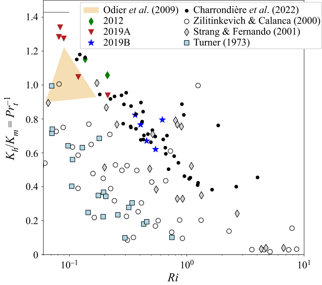
as functions of height that also increase linearly with $z$, in the range of considered heights. This behaviour suggests a logarithmic variation of $\bar {u}$ in this part of the outer region. Indeed, the experiments indicate such a trend, as is shown in the inset of figure 3(c). In figure 7, the ratio $K_h/K_m=Pr_t^{-1}$ is plotted as a function of $Ri$. This ratio decreases from nearly $1.4$ ($Pr_t\approx {0.7}$) at near neutral conditions to $\approx 0.4$ ($Pr_t\approx 2.5$) at $Ri\approx 1$. Data from Charrondière et al. (Reference Charrondière, Brun, Cohard, Sicart, Obligado, Biron, Coulaud and Guyard2022) and other published data have been added for comparison. These are: laboratory turbulent gravity current data (Turner Reference Turner1973), stratified shear layer data (Strang & Fernando Reference Strang and Fernando2001), and atmospheric surface layer data (Zilitinkevich & Calanca Reference Zilitinkevich and Calanca2000). All show a decrease of $K_h/K_m$ with increasing gradient Richardson number $Ri$, but none reaches the turbulent Prandtl number value $Pr_t\eqsim 0.7$ as $Ri\longrightarrow 0$. The ratios obtained from laboratory gravity current and from atmospheric surface layer (Turner Reference Turner1973; Zilitinkevich & Calanca Reference Zilitinkevich and Calanca2000) are mostly below the present katabatic jet values, whereas those obtained from a free shear layer by Strang & Fernando (Reference Strang and Fernando2001) are in the range of the present values. As is shown in Turner (Reference Turner1973), the ratio depends on the critical value of $Rf$ with the higher ratios being associated with higher $Rf_{crit}$, noting that in the present experiments, $Rf$ is replaced by $R_m$ (see mixing efficiency below). In laboratory gravity currents, Reynolds numbers are smaller than in the present case, and in a boundary layer, stability conditions differ from those of a free shear region. For a very stable boundary layer, Kondo, Kanechika & Yasuda (Reference Kondo, Kanechika and Yasuda1978) concluded that when $Ri>1$, the turbulent Prandtl number $Pr_t$ is always higher than 1, with no clear trend as $Ri$ increases. The present data (figure 7) show a clear increase of $Pr_t$ with increasing $Ri$. Anderson (Reference Anderson2009) proposed momentum transport by internal waves as a possible mechanism to explain the observed trends at very large $Ri$, which was not possible to confirm from our data.

Figure 6.

Variation with height of (a) momentum eddy coefficient $K_m$, (b) heat eddy coefficient $K_h$, (c) momentum mixing length $l_m$ (see (5.2)), and (d) mixing length of heat $l_h$ (see (5.3)), in the outer region of the three katabatic events defined in § 3. The height is measured from the maximum wind velocity height $z_j$, and both axes are normalized by the integral scales $h$ and $U_{exp}$ provided in table 1.

Figure 7.

Ratio of eddy coefficients of heat and momentum as a function of the gradient Richardson number. The data from the 2012, 2019A and 2019B katabatic events are the coloured markers. Black dots represents all the other events from the 2019 field experiment (Charrondière et al. Reference Charrondière, Brun, Cohard, Sicart, Obligado, Biron, Coulaud and Guyard2022). The short horizontal bar indicates a turbulent Prandtl number equal to 0.7. The data of Strang & Fernando (Reference Strang and Fernando2001) are for a laboratory stratified shear layer, and the data of Zilitinkevich & Calanca (Reference Zilitinkevich and Calanca2000) are for a stratified atmospheric surface layer, extracted from Zilitinkevich (Reference Zilitinkevich1970) and Kondo et al. (Reference Kondo, Kanechika and Yasuda1978). The data corresponding to Turner (Reference Turner1973) are for a laboratory gravity currents extracted from Ellison & Turner (Reference Ellison and Turner1960). The results of $Pr_t^{-1}$ versus $Ri$ of Odier et al. (Reference Odier, Chen, Rivera and Ecke2009) have been determined from their figures, and those referred to as Charrondière et al. (Reference Charrondière, Brun, Cohard, Sicart, Obligado, Biron, Coulaud and Guyard2022) calculated from their data set.

Mixing efficiency expresses removal of turbulence kinetic energy (TKE) by buoyancy forces with respect to TKE production. In a stationary katabatic wind, local equilibrium can be assumed so that the turbulence kinetic energy budget (Stull Reference Stull1988) can be written as

(5.4)\begin{equation} -\overline{u'w'}\,\frac{\partial \bar{u}}{\partial z} + \frac{g}{\bar{\theta}}\,\overline{w'\theta'} \cos \alpha -\frac{g}{\bar{\theta}}\,\overline{u'\theta'} \sin \alpha \approx\varepsilon . \end{equation}

Advective and transport terms are indeed negligible with respect to mechanical shear, buoyancy and dissipation terms (see e.g. Charrondière et al. Reference Charrondière, Brun, Sicart, Cohard, Biron and Blein2020, for katabatic winds), which is not the case for the mean flow in the momentum and heat equations (see § 2). The negligible contribution of advective terms in the TKE budget in both the $x$ and $z$ directions has also been shown, for example, by Nadeau et al. (Reference Nadeau, Pardyjak, Higgins, Huwald and Parlange2013). While TKE is produced by shear and dissipated by viscosity, removal or supply of turbulence energy by buoyancy forces depends on the signs of the sensible heat flux terms.

The flux Richardson number $Rf$ as defined by Turner (Reference Turner1973), also known as mixing efficiency (Grachev et al. Reference Grachev, Andreas, Fairall, Guest and Persson2015), is the ratio of removal of energy by buoyancy forces to its production by shear; $Rf$ has also been expressed as the ratio of the buoyancy terms to production by shear in the turbulence kinetic energy budget (Stull Reference Stull1988; Charrondière et al. Reference Charrondière, Brun, Sicart, Cohard, Biron and Blein2020). Grachev et al. (Reference Grachev, Andreas, Fairall, Guest and Persson2015) further suggest $Rf$ as the ratio of removal of TKE by buoyancy forces to viscous dissipation. More generally, mixing efficiency is defined as removal of energy by mixing (loss of TKE) to its production, which can be by shear or stirring (Linden Reference Linden1979; Hopfinger Reference Hopfinger1987). Mixing efficiency, as defined by Richardson (Reference Richardson1920), is irreversible loss of energy by mixing to energy supply by eddies that can be shear and/or convection. Richardson (Reference Richardson1920) already mentions that in the atmosphere, this ratio of loss of energy by mixing to its production is approximately 0.3. It has been shown that in the outer region of katabatic jets over steep slopes, the along-slope component of the turbulent heat flux $\overline {u'\theta '}$ produces TKE (Horst & Doran Reference Horst and Doran1988; Oldroyd et al. Reference Oldroyd, Pardyjak, Higgins and Parlange2016; Charrondière et al. Reference Charrondière, Brun, Sicart, Cohard, Biron and Blein2020). This is also observed here, where figure 5(c) shows that the flux $\overline {u'\theta '}$ is of the same order as $\overline {w'\theta '}$ . Thus the physically meaningful definition of mixing efficiency or mixing ratio, here denoted by $Rm$, is removal of energy by mixing to its production by shear and buoyancy, i.e.

(5.5)\begin{equation} Rm = \frac{\dfrac{g}{\bar{\theta}}\,\overline{w^{\prime}\theta^{\prime}}\cos \alpha}{\overline{u^{\prime}w^{\prime}}\,\dfrac{\partial \bar{u}}{\partial z} + \dfrac{g}{\theta}\,\overline{u^{\prime}\theta^{\prime}}\sin \alpha} = Rf \left(1+\left(\frac{g}{\bar{\theta}}\,\overline{u'\theta'}\sin \alpha\right) \left(\overline{u'w'}\, \frac{\partial \bar{u}}{\partial z}\right)^{{-}1}\right)^{{-}1} . \end{equation}

When the slope angle $\alpha$ tends to $0$, the mixing efficiency reduces to the classical expression of the flux Richardson number, $Rm\to Rf = (g \overline {w^{\prime }\theta ^{\prime }}/\bar {\theta })/ (\overline {u^{\prime }w^{\prime }}\,\partial \bar {u}/\partial z)$ (Turner Reference Turner1973; Stull Reference Stull1988).

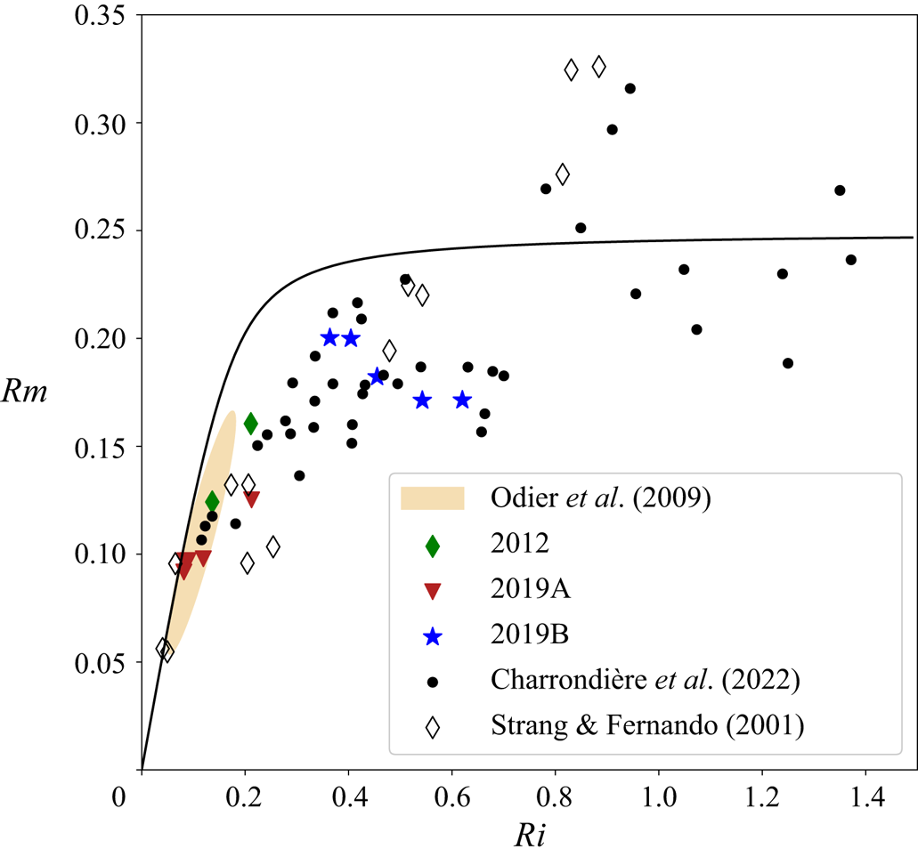
In figure 8, $Rm$ is plotted versus $Ri$. At low values of $Ri$, $Rm$ increases nearly proportional to $Ri$. Then the mixing efficiency reaches rapidly a threshold value of $Rm \approx 0.25$ at $Ri\approx 0.5$. Turbulence models of the relationship between $Rf$ and $Ri$ suggest an asymptotic value of $Rf$ at high $Ri$. In the level 2 model of Mellor & Yamada (Reference Mellor and Yamada1974), an asymptotic value $Rf {\sim}eq 0.25$ is approached for $Ri>0.3$, for example. This semi-empirical model has been adjusted with neutral atmospheric data, but has been shown to be consistent with stratified surface layers. As seen in figure 8, at large $Ri$ there is a large spread in mixing efficiency, varying from $0.2$ to $0.32$ for all the katabatic events of the 2019 field experiment. In the laboratory stratified shear layer (Strang & Fernando Reference Strang and Fernando2001, also shown in figure 8), values range up to $0.4$, and in nature, Pardyjak, Monti & Fernando (Reference Pardyjak, Monti and Fernando2002) obtained values in the range 0.4–0.5. Measured mixing efficiencies at large values of $Ri$ generally show a decreasing trend with increasing $Ri$ (Linden Reference Linden1979; Hopfinger Reference Hopfinger1987). This is not observed in katabatic winds, either because $Ri$ values are too low or because turbulence is maintained. In decaying stratified turbulence, a decrease of $Rm$ ($Rf$) with increasing $Ri$ is to be expected.

Figure 8.

Variation of mixing efficiency $Rm$ with gradient Richardson number $Ri$. Coloured symbols correspond to data from the 2012, 2019A and 2019B katabatic events. Black dots represents all the other events from the 2019 field experiment (Charrondière et al. Reference Charrondière, Brun, Cohard, Sicart, Obligado, Biron, Coulaud and Guyard2022). The range of $Rm$ determined with the data of Odier et al. (Reference Odier, Chen, Rivera and Ecke2009) is represented by the filled oval. Empty diamond symbols represent data of the laboratory stratified shear layer of Strang & Fernando (Reference Strang and Fernando2001). The black continuous line is the empirical solution of the level 2 model by Mellor & Yamada (Reference Mellor and Yamada1974). The results of $Rm$ versus $Ri$ of Odier et al. (Reference Odier, Chen, Rivera and Ecke2009) have been determined from the fluxes given in their paper, and those of Charrondière et al. (Reference Charrondière, Brun, Cohard, Sicart, Obligado, Biron, Coulaud and Guyard2022) calculated from their data.

5.2. Inner region

The inner, boundary region of the jet ($z< z_j$) is relatively thin, and velocity data are available only for the 2019B katabatic event obtained with the 3-D Pitot tube (§ 3). The measured velocities have been shown to follow a logarithmic law with a slight correction due to gravity effects on $\overline {u'w'}$ (Charrondière et al. Reference Charrondière, Brun, Cohard, Sicart, Obligado, Biron, Coulaud and Guyard2022, their figure 10). The corresponding velocity gradient is then $\partial \bar {u}/\partial z = u_*(\kappa z)^{-1} - a u_* (2\kappa )^{-1}$, with friction velocity $u_* = 0.16$ m s$^{-1}$, von Kármán constant $\kappa = 0.38$, and gravity correction $a=1.9$ m$^{-1}$ in the present case. This corrected logarithmic law is here used to infer turbulent mixing properties, i.e. eddy viscosity $K_m$, mixing length $l_m$, and heat fluxes, together with the gradient Richardson number $Ri$ in this inner region. The gradient Richardson number increases from $Ri\approx {0.01}$ near the ground to $Ri\approx {0.1}$ at the highest measurement level captured by the 3-D Pitot tube ($z/z_j = 0.66$). Note that the logarithmic law extended over almost the whole height of the inner layer, implying that an equivalent boundary layer thickness would extend well beyond $z_j$.

Turbulent dissipation was shown in Charrondière et al. (Reference Charrondière, Brun, Cohard, Sicart, Obligado, Biron, Coulaud and Guyard2022, their figure 10) to follow roughly the standard decreasing trend as observed in a turbulent boundary layer under neutral conditions on a flat surface, $\varepsilon = u_*^3/(\kappa z)$ (Pope Reference Pope2000). Moreover, the consumption of TKE by buoyancy (note that in the inner region of the jet, $\overline {u'\theta '}$ is of sign opposite to that in the outer region) is weak in this region where the local Obukhov length $L_O=- (\bar {\theta }/\kappa g) (u_*^3/ \overline {(w'\theta ')_s})$ (Stull Reference Stull1988), estimated at the first sonic measurement level close to $z_j \approx 0.42$ m, is $L_O\approx 12$ m. These observations support the assumption that the mixing length $l_m$ grows linearly with height at the same rate as the dissipation length, i.e. $l_m$ proportional to $\kappa z$, as expected from the theory of neutral turbulent boundary layers (e.g. Pope Reference Pope2000). The turbulent viscosity is $K_m ={l_m}^2\,\partial \bar {u}/\partial z= \kappa u_* z (1-az/2)$, and ranges from $2\times 10^{-3}$ m$^{2}$ s$^{-1}$ to approximately $10^{-2}$ m$^{2}$ s$^{-1}$. The gravity correction $az/2$ reaches only 0.26 at the highest measurement level, so a linear variation of $K_m$ with $z$ is indeed a good approximation for both the inner region and the lower part of the outer-layer region of a katabatic jet (in agreement with Grisogono & Oerlemans Reference Grisogono and Oerlemans2001; Brun et al. Reference Brun, Blein and Chollet2017; Charrondière et al. Reference Charrondière, Brun, Sicart, Cohard, Biron and Blein2020, for example).

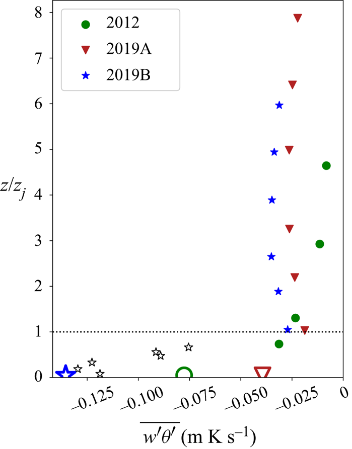
Given the low values of $Ri$ in this inner region, it can be assumed that the ratio $K_h/K_m$ is close to 1. From the temperature gradient $\partial \bar {\theta } /\partial z$ and the value of $K_m$ determined from the Pitot tube measurements, we obtained an estimation of the turbulent flux of sensible heat $\overline {w'\theta '}$ in the lower part of the jet at the 6 measurement heights in the 2019B event. These values are shown in figure 9, along with the turbulent sensible heat fluxes measured with sonic anemometers in the outer region of the jet. In the outer mixing region, turbulent heat fluxes are nearly constant compared with the variations in the boundary region where $\overline {w'\theta '}$ varies by a factor of 3–4.

Figure 9.

Turbulent sensible heat fluxes $\overline {w'\theta '}$ for the three katabatic events defined in § 3. Filled symbols are from sonic anemometry measurements. Empty small stars are estimated from Cobra data of momentum flux $\overline {u'w'}$, with the hypothesis that $K_h/K_m =1$ in this inner layer of the 2019B event. The big open symbols are the turbulent fluxes $\overline {(w'\theta ')}_s$, estimated from (2.9), with $m=0$ and $n=1/3$, and measured integrated buoyancy flux $B$.

Figure 9 also shows the estimates of $\overline {(w'\theta ')}_s$ from the depth-integrated model (§ 2 and table 1) for the three katabatic events, giving heat fluxes ranging from $Q_s\approx -43$ W m$^{-2}$ to $Q_s\approx -145$ W m$^{-2}$, depending on the event (table 1). The value of the surface sensible heat flux obtained in the 2019B event with the depth-integrated model is consistent with the inner layer values of the heat flux evaluated with the assumption $K_h/K_m \approx 1$. In experimental katabatic wind studies, $Q_s$ is rarely known and is often determined from the first measurement level that is above the surface. Thus, considering the strong variation of the heat flux in the boundary region, these measured heat fluxes above the surface are likely to underestimate considerably the surface heat flux.

The mixing efficiency $Rm$ in the inner region will remain small because $Ri$ remains small, so the temperature in this part of the flow can be considered close to a passive scalar field in terms of turbulence. It may be noted that the along-slope turbulent heat flux reverses sign close to the maximum wind velocity height (Charrondière et al. Reference Charrondière, Brun, Sicart, Cohard, Biron and Blein2020), thus the mixing efficiency is the transfer to turbulence potential energy (TPE) with respect to the production by shear reduced by the along-slope component of the buoyancy term of the TKE budget.