1. Introduction
Birds can actively control the gliding aerodynamic performance through the sweep morphing of their wings. The sweep morphing wings enable the aerodynamic shape to be reconfigured dynamically, thereby integrating high lift and efficiency (Lentink et al. Reference Lentink2007; Harvey et al. Reference Harvey, Gamble, Bolander, Hunsaker, Joo and Inman2022b ), and also balancing flight stability and manoeuvrability (Harvey et al. Reference Harvey, Baliga, Wong, Altshuler and Inman2022a ; Harvey & Inman Reference Harvey and Inman2022). The sweep morphing wings inspire the design of multifunctional aircraft, which have significant advantages in scenarios with dense obstacles (Ajanic et al. Reference Ajanic, Feroskhan, Mintchev, Noca and Floreano2020). The fundamental problems of wing morphing are revealing the response characteristics of unsteady aerodynamic forces and reducing the negative effects of unsteady aerodynamic loadings on the lifting surfaces (McCroskey Reference McCroskey1982).
The sweep morphing and the streamwise velocity adjusting of the wing, both the same type of surging process (Chow & Huang Reference Chow and Huang1982; Katz, Yon & Rogers Reference Katz, Yon and Rogers1996; Huang et al. Reference Huang, Wu, Jeng and Chen2001; Choi, Colonius & Williams Reference Choi, Colonius and Williams2015), exhibit similar lift response and vortex dynamics. Mulleners, Mancini & Jones (Reference Mulleners, Mancini and Jones2017) experimentally measured the lift coefficient of a flat-plate wing with an aspect ratio of 6 at an angle of attack of
 $30^{\circ }$
during two streamwise accelerations. One is the linear acceleration from rest to a constant velocity, while the other is the linear acceleration from that constant velocity to 1.5 times as much. The two lift-coefficient histories are similar except in the early stage of acceleration, when the difference in the lift coefficient is due to the presence of near-wake vortices in the acceleration from a non-stationary flow. The lift coefficient first undergoes an irregular oscillating transient and then converges to a steady value at large time. The oscillating lift coefficient is characterised by the local maximum lift overshoot and the decaying successive lift peaks. The principal frequency of oscillating lift coefficient corresponds to a Strouhal number between 0.25 and 0.27. Chen, Colonius & Taira (Reference Chen, Colonius and Taira2010) numerically simulated the continuous acceleration of a flat-plate aerofoil from rest at the same angle of attack. The results show that the lift coefficient, without ceasing the acceleration, still has similar oscillating characteristics including local maximum lift overshoot and successive lift peaks. Differently, at large time, the lift coefficient exhibits periodic oscillations, which are related to the absence of three-dimensional effects that would otherwise maintain a steady state (Zhang et al. Reference Zhang, Hayostek, Amitay, Burtsev, Theofilis and Taira2020). For the case of linear deceleration to rest, the lift coefficient initially displays a local maximum lift undershoot to negative value range. Subsequently, it crosses zero and recovers to a positive peak value (Lua, Lim & Yeo Reference Lua, Lim and Yeo2011).
The wing surging may cause uncontrollable additional heaving before the new trim state is reached. This passive heaving serves as a perturbation to flight stability (Thomas & Taylor Reference Thomas and Taylor2001) as well as gaze stability (Warrick, Bundle & Dial Reference Warrick, Bundle and Dial2002; Pete et al. Reference Pete, Kress, Dimitrov and Lentink2015). The lift change induced by the wing surging potentially excites or amplifies dynamic stall, flutter and buffeting (McCroskey Reference McCroskey1982). To suppress these adverse effects, it is necessary to reduce the local maximum lift over/undershoot. First, increasing the acceleration duration facilitates the low-heaving start of the wing. Mancini et al. (Reference Mancini, Manar, Granlund, Ol and Jones2015) and Stevens et al. (Reference Stevens2017) compare the slow and fast start modes with travel of 6 and 1 chord lengths, respectively, for a linearly accelerating flat-plate wing. They find that the slow start mode produces a lower local maximum lift overshoot during a longer acceleration duration. The slow start mode also avoids the secondary peak lift that occurs in the fast start mode. Second, nonlinear acceleration provides the flexibility to design kinematics point by point. When applying the power law (Pullin & Wang Reference Pullin and Wang2004) to accelerate a flat-plate aerofoil, adjusting the power exponent changes the local maximum lift overshoot and its timing (Chen et al. Reference Chen, Colonius and Taira2010). Third, reducing the angle of attack can reduce the local maximum lift overshoot and the amplitude of the subsequent oscillating lift coefficient when the wing accelerates from rest (Chen et al. Reference Chen, Colonius and Taira2010; Mancini et al. Reference Mancini, Manar, Granlund, Ol and Jones2015). Other effective strategies include the tuning of wing inertial properties (Suzuki, Okada & Yoshino Reference Suzuki, Okada and Yoshino2019).
The unsteady lift generated by the surging wings originates from the inertial and the circulatory effects (Mancini et al. Reference Mancini, Manar, Granlund, Ol and Jones2015; Oh et al. Reference Oh, Lee, Park, Choi and Kim2020). The lift during the accelerating start of the wing, which includes the local maximum lift overshoot, can be decomposed into the contributions of the added mass and the growing leading edge vortices (LEVs). Pitt Ford & Babinsky (Reference Pitt Ford and Babinsky2013) derive a formula for the added-mass lift component of an accelerating flat-plate aerofoil in the attached flow state. By applying this lift formula, Mancini et al. (Reference Mancini, Manar, Granlund, Ol and Jones2015) conclude that the circulatory component related to the LEVs dominates the lift of the accelerating wing compared with the added-mass component. The lift after the accelerating start of the wing, which includes the decay or growth of the successive lift peaks under large angles of attack, is completely determined by the sequentially evolving LEVs, since the added-mass force becomes zero. Therefore, controlling the evolution of the LEVs is essential for reducing the local maximum lift over/undershoot of the sweep morphing wing (Dickinson & Götz Reference Dickinson and Götz1993; Li & Wu Reference Li and Wu2015). In the experiment of linear accelerating flat-plate wing (Mulleners et al. Reference Mulleners, Mancini and Jones2017), the local maximum lift overshoot occurs when the initial LEVs reach the scale of wing chord. The decay of the successive lift peaks is closely related to the downstream convection of the region, where the leading and trailing edge vortices (TEVs) form and interact. The oscillating lift coefficient correlates with the alternating shedding of the LEVs and TEVs. Stevens et al. (Reference Stevens2017) report the vortex core spacing in the early stage as well as the relative convective velocity of the LEVs and TEVs. In addition, the duration of the accelerating start does not affect the trajectory of the LEVs, but the fast start mode generates the LEVs with more vorticity and more coherent structure (Mancini et al. Reference Mancini, Manar, Granlund, Ol and Jones2015). The vortex dynamics of decelerating wings can be observed in the perching manoeuvre of birds, where the wing deceleration is superimposed with other forms of motion (Polet, Rival & Weymouth Reference Polet, Rival and Weymouth2015; Adhikari et al. Reference Adhikari, Loubimov, Kinzel and Bhattacharya2022).
The transient development of the LEVs during wing surging is associated with varied amount and distribution of vorticity in the pre-surging flow (Mulleners et al. Reference Mulleners, Mancini and Jones2017). The initial vorticity carries the historical information of the flow, which is naturally encoded into the subsequent transient, as reflected in similar dynamic processes (Strangfeld et al. Reference Strangfeld, Müller-Vahl, Nayeri, Paschereit and Greenblatt2025; Mulleners & Raffel Reference Mulleners and Raffel2013; Toppings & Yarusevych Reference Toppings and Yarusevych2025). Moreover, the initial near-wake vorticity behind the wing has a finite convection velocity (Rival, Prangemeier & Tropea Reference Rival, Prangemeier and Tropea2009), thereby limiting the growth of the LEVs and changing their proximity to the wing surface (Green & Galbraith Reference Green and Galbraith1995; Mulleners et al. Reference Mulleners, Mancini and Jones2017). In previous studies on wing acceleration, the initial flow is either stationary or steady. Conversely, the pre-morphing flow around the in-flight avian wings is usually in an unsteady separated condition (Linehan & Mohseni Reference Linehan and Mohseni2020; Nair & Goza Reference Nair and Goza2022), as a result of combining the sweep angle, aspect ratio and angle of attack of the wing (Zhang et al. Reference Zhang, Hayostek, Amitay, Burtsev, Theofilis and Taira2020; Zhang & Taira Reference Zhang and Taira2022). The formation of this unsteady separation is affected by the spanwise transport of the LEVs and the downwash effect of the tip vortices. For the fully developed unsteady separated flow, the evolution and interaction of the vortex structures generate lift that changes regularly with time (Taira & Colonius Reference Taira and Colonius2009; Huang et al. Reference Huang, Venning, Thompson and Sheridan2015; Ribeiro et al. Reference Ribeiro, Neal, Burtsev, Amitay, Theofilis and Taira2023). However, the time-dependent lift response of the sweep morphing from the unsteady separation remains unclear.
The aim of this work is to investigate the lift response of the sweep morphing wing in a fully developed unsteady separated state, reveal the physical composition of the local maximum lift over/undershoot and propose a predictive model for the time-dependent lift during sweep morphing. The avian-inspired wing model adopted in this work consists of an inner (arm) and an outer (hand) wing. The local sweep angles of the inner and outer wings are morphed by actuating the shoulder and wrist joints (Liu et al. Reference Liu, Kuykendoll, Rhew and Jones2006; Harvey & Inman Reference Harvey and Inman2022), which is referred to as local sweep morphing (Wang et al. Reference Wang, Liu, Xu and Wang2022). The remainder of this paper is structured as follows. The morphing wing model and the unsteady numerical simulation method are described in § 2. The effects of different local sweep angles on the aerodynamic performance, the unsteady aerodynamics of the local sweep morphing and the time-dependent lift model are presented and discussed in § 3. Finally, the conclusions are summarised in § 4.
2. Numerical model and method
2.1. Local sweep morphing wing
The morphing wing model consists of an inner and an outer wing. Its wing planform simplified from that of northern goshawk (Ajanic et al. Reference Ajanic, Feroskhan, Mintchev, Noca and Floreano2020). The basic ways of sweep morphing include shearing and rotating (Diederich Reference Diederich1951). The shear morphing ensures that the wing chords parallel to the symmetric plane are constant. In contrast, the rotate morphing ensures that the wing chords perpendicular to the leading edge or the quarter-chord line are constant. The rotate morphing simultaneously alters span length and wing area, while the shear morphing keeps them unchanged. To identify the effects of the sweep angle, we use the shearing way for conducting the local sweep morphing. Mind that this morphing way does not fully conform to biological characteristics, as birds alter their local sweep angles by rotating about the shoulder and wrist joints. Throughout the morphing, both the inner and outer wings are consistently within the same wing plane. The schematic diagram of the unilateral local sweep morphing wing is shown in figure 1. The
 $x$
-axis,
 $y$
-axis and
 $z$
-axis of the global coordinate system represent the streamwise, spanwise and vertical directions, respectively. The tangential direction from the projection of the
 $x\hbox{-}$
axis onto the wing plane is denoted as the
 $s\hbox{-}$
axis, and the normal direction of the wing plane is represented by the
 $n\hbox{-}$
axis. The local sweep angles of the inner and outer wings are
 ${ \Lambda }_{\textit{iw}}$
and
 ${ \Lambda }_{\textit{ow}}$
, respectively. The local sweep angles are defined by the angles between the half-chord lines and the spanwise axis (Anderson Reference Anderson2010), and are assigned a positive sign when the local sweep is backward. The semi-span
 ${b}_{\textit{iw}}$
of the inner wing equals the semi-span
 ${b}_{\textit{ow}}$
of the outer wing. Both semi-spans are identical to the maximum chord
 ${c}_{\textit{max}}$
at the wing root, leading to an aspect ratio of 4.40 for a pair of local sweep morphing wings. The wing geometry is detailed in Appendix A and is also presented in our previous work (Wang et al. Reference Wang, Liu, Xu and Wang2022). The morphing wing is placed in a fluid with a density of
 $\rho$
and a kinematic viscosity of
 $\nu$
. The velocity of the uniform oncoming flow upstream of the wing is
 ${U}_{\infty }$
. The geometric angle of attack
 $\alpha$
is set to
 $30^\circ$
for producing the initial flow of unsteady separation (Mulleners et al. Reference Mulleners, Mancini and Jones2017).
Schematic diagram of the local sweeping wing: (a) wing morphing; (b) wing planform.

For the local sweep morphing in the shearing form, the spanwise position of any point on the inner and outer wings remains unchanged. In the wing plane, the tangential displacements of the points on the inner and outer wings along the
 $s\hbox{-}$
axis depend on their spanwise positions and the local sweep angles. At the dimensionless time
 $t$
, the tangential displacements
 $\Delta s_{\textit{iw}}$
and
 $\Delta s_{\textit{ow}}$
at the spanwise positions
 ${y}_{\textit{iw}}$
on the inner wing and
 ${y}_{\textit{ow}}$
on the outer wing are respectively
 \begin{align} \Delta {{s}_{\textit{iw}}}\left ( t \right ) &={{y}_{\textit{iw}}}\left [ \tan {{ \Lambda }_{\textit{iw}}}\left ( t \right )-\tan {{ \Lambda }_{\textit{iw}}}\left ( {{t}_{0}} \right ) \right ], \quad{{t}_{0}}\leqslant t\leqslant {{t}_{f}}, \end{align}
 \begin{align} \Delta {{s}_{\textit{ow}}}\left ( t \right ) & =\left ( {{y}_{\textit{ow}}}-{{b}_{\textit{iw}}} \right )\left [ \tan {{ \Lambda }_{\textit{ow}}}\left ( t \right )-\tan {{ \Lambda }_{\textit{ow}}}\left ( {{t}_{0}} \right ) \right ],\quad {{t}_{0}}\leqslant t\leqslant {{t}_{f}}, \end{align}
where
 $t_0$
is the dimensionless initial moment and
 $t_f$
is the dimensionless final moment of the local sweep morphing. In this study, given the reference length
 $l_{\textit{ref}}={\gamma }{c}_{max }$
and velocity
 $U_{\textit{ref}}={U}_{\infty }$
, the reference time is defined as
 $\tau _{\textit{ref}}={{\gamma }{c}_{max }}/{{U}_{\infty }}$
, with the scale factor
 ${\gamma }=10/7$
.
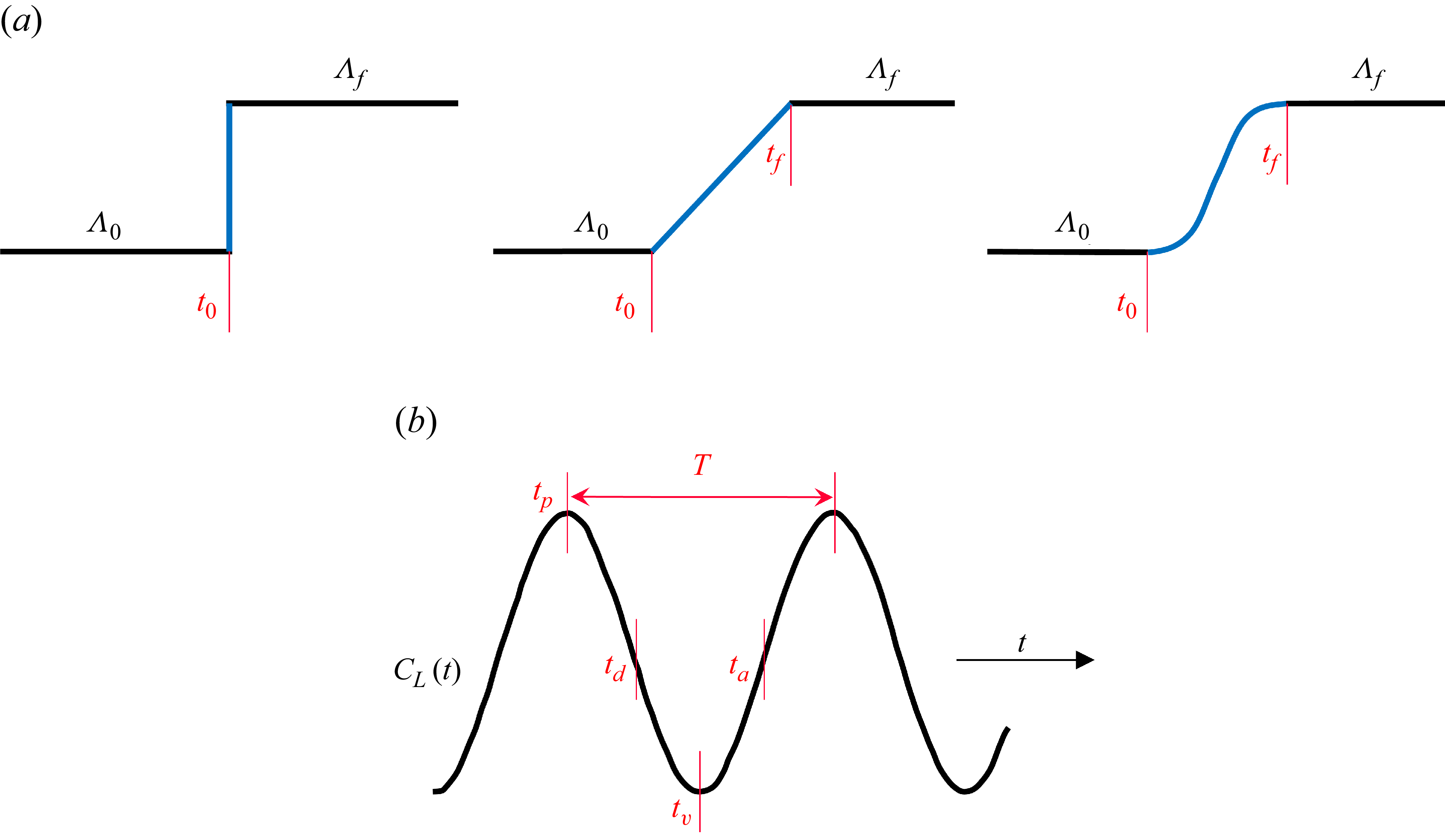
The local sweep morphing is implemented by three typical kinematics based on the step, linear and nonlinear functions, as shown in figure 2. The step and linear morphing kinematics exhibit discontinuities at the initial and final moments of the morphing. The nonlinear morphing kinematics assumes a sinusoidal form, which maintains smoothness throughout the entire morphing (Zhu et al. Reference Zhu, Liu, Liu, Zou and Wu2015). From the initial sweep angle
 ${ \Lambda }_{0}$
to the final sweep angle
 ${ \Lambda }_{f}$
, the expressions of the three morphing kinematics are respectively
 \begin{align} {{ \Lambda }_{\textit{step}}}\left ( t \right ) & =\left \{ \begin{matrix} {{ \Lambda }_{0}}, & t\lt {{t}_{0}}, \\ {{ \Lambda }_{f}}, & t\geqslant {{t}_{0}}, \\ \end{matrix} \right.\end{align}
 \begin{align} {{ \Lambda }_{\textit{linear}}}\left ( t \right ) & =\left \{ \begin{matrix} {{ \Lambda }_{0}}, & t\lt {{t}_{0}}, \\ \displaystyle \frac {{{ \Lambda }_{f}}-{{ \Lambda }_{0}}}{{{t}_{f}}-{{t}_{0}}}\left ( t-{{t}_{0}} \right )+{{ \Lambda }_{0}}, & {{t}_{0}}\leqslant t\leqslant {{t}_{f}}, \\ {{ \Lambda }_{f}}, & t\gt {{t}_{f}}, \\ \end{matrix} \right.\end{align}
 \begin{align} {{ \Lambda }_{\textit{sine}}}\left ( t \right ) & =\left \{ \begin{matrix} {{ \Lambda }_{0}}, & t\lt {{t}_{0}}, \\ \displaystyle \frac {{{ \Lambda }_{f}}-{{ \Lambda }_{0}}}{2}\sin \left (\vphantom{\frac {\pi t}{{{t}_{f}}-{{t}_{0}}}-\frac {\pi }{2}\frac {{{t}_{f}}+{{t}_{0}}}{{{t}_{f}}-{{t}_{0}}}} \frac {\pi t}{{{t}_{f}}-{{t}_{0}}}-\frac {\pi }{2}\frac {{{t}_{f}}+{{t}_{0}}}{{{t}_{f}}-{{t}_{0}}} \right )+\frac {{{ \Lambda }_{f}}+{{ \Lambda }_{0}}}{2}, & {{t}_{0}}\leqslant t\leqslant {{t}_{f}}, \\ {{ \Lambda }_{f}}, & t\gt {{t}_{f}} .\\ \end{matrix} \right.\end{align}
Implementations of local sweep angle morphing: (a) three morphing kinematics; (b) four typical morphing starts and the reference time of morphing duration. In panel (a), the three morphing kinematics
 $ \Lambda (t)$
presented from left to right are the step, linear and nonlinear sinusoidal morphing kinematics, respectively. Panel (b) shows the pre-morphing oscillating lift coefficient with a period of
 $T$
, and four morphing starts including the peak moment
 $t_p$
, the descending-mean moment
 $t_d$
, the valley moment
 $t_v$
and the ascending-mean moment
 $t_a$
.

All of these morphing kinematics are applicable to both forward sweep morphing and backward sweep morphing.
The start of the local sweep morphing can be assigned at the moment corresponding to any instantaneous lift. As shown in figure 2(b), the peak moment
 $t_p$
, the descending-mean moment
 $t_d$
, the valley moment
 $t_v$
and the ascending-mean moment
 $t_a$
of pre-morphing lift coefficient are chosen to investigate the differences in the lift response during the morphing under various morphing starts. In addition, the duration of the local sweep morphing is also a crucial factor affecting the lift response. The period
 $T$
of the pre-morphing oscillating lift coefficient is taken as a time scale for measuring the morphing duration. The effect of the morphing durations ranging from 1 to 4 times the period
 $T$
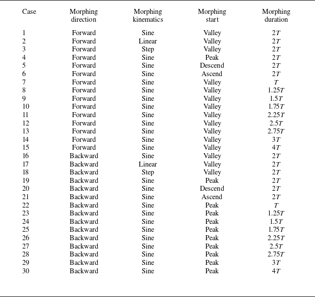
on the lift response is evaluated. Table 1 summarises all the cases of the local sweep morphing wing in this work.
Set-up of the local sweep morphing wings.

The lift response of local sweep morphing depends on the unsteady aerodynamics of the fixed wing with different local sweep angles before morphing. In this study, the fixed wing is not specified any additional motion, only fixed at the considered angle of attack to encounter the uniform free stream. According to the work of Harvey & Inman (Reference Harvey and Inman2022), we investigate the aerodynamic characteristics of the fixed wing with different local sweep angles, where the sweep angle of the inner wing ranges from
 $-20^{\circ }$
to
 $20^{\circ }$
and that of the outer wing ranges from
 $-40^{\circ }$
to
 $40^{\circ }$
. The cases of the fixed wing with different local sweep angles are presented in table 2.
Set-up of the fixed wings with different local sweep angles.

2.2. Numerical method
The wing morphing falls within the category of moving boundary problems. For the local sweep morphing investigated in this paper, we use the immersed boundary method subject to the continuity hypothesis for its treatment. Under the framework of the immersed boundary method, the three-dimensional viscous incompressible Navier–Stokes equations describing the flow around the local sweeping wing are as follows:
 \begin{align} \boldsymbol{\nabla }\boldsymbol{\cdot }\boldsymbol{u} &=0, \end{align}
 \begin{align} \frac {\partial \boldsymbol{u}}{\partial t} + \boldsymbol{u} \boldsymbol{\cdot }\boldsymbol{\nabla }\boldsymbol{u} & = -\boldsymbol{\nabla }p + \frac {1}{{Re}} {{{\nabla} }^{2}}\boldsymbol{u} + {{\boldsymbol{f}}_{\!m}}, \end{align}
where
 $\boldsymbol{u}$
is the dimensionless velocity vector, normalised by the oncoming flow velocity
 ${U}_{\infty }$
, and
 $p$
is the dimensionless pressure, normalised by
 ${\rho } U_{\infty }^{2}$
. The Reynolds number is defined as
 ${\textit{Re}} = {{{U}_{\infty }}{({\gamma }{c}_{\textit{max}})}}/{{\nu } }$
, based on the oncoming flow velocity
 ${U}_{\infty }$
and the scaled maximum chord
 $\gamma {c}_{\textit{max}}$
. The external body force
 ${\boldsymbol{f}}_{\!m}$
reflects the effect of the local sweep morphing wing on the surrounding fluid. It is worth noting that the non-dimensionalisation of the Navier–Stokes equations is only applicable for cases where the density appropriately scales. These equations have also been used to investigate the unsteady flows in bio-locomotion with Reynolds numbers of
 $O(10^2)$
or
 $O(10^3)$
(Borazjani & Sotiropoulos Reference Borazjani and Sotiropoulos2008; Brunton, Rowley & Williams Reference Brunton, Rowley and Williams2013; Liu et al. Reference Liu, Ren, Dong, Akanyeti, Liao and Lauder2017; Kim, Lee & Kim Reference Kim, Lee and Kim2019).
We consider that the separation point of the morphing flat-plate wing with a sharp leading edge is insensitive to the Reynolds number and that the unsteady flow is dominated by the Strouhal number (Ho et al. Reference Ho, Nassef, Pornsinsirirak, Tai and Ho2003; Buchholz & Smits Reference Buchholz and Smits2006). Hence, the Reynolds number is specified as 300, which allows the trade-off between sufficing grid resolution and resolving unsteady aerodynamics in bio-locomotion simulations according to the literature by Taira & Colonius (Reference Taira and Colonius2009), Shyy et al. (Reference Shyy, Trizila, Kang and Aono2009), Li & Nabawy (Reference Li and Nabawy2024). Note that the Reynolds number is lower than actual values in avian flight, although its effects on the basic characteristics and lift generation of large-scale vortex structures remain limited (Liu, Wang & Liu Reference Liu, Wang and Liu2024).
The immersed boundary method in a discrete stream function formulation is used to solve the flow equations. The second-order finite-volume method is employed for spatial discretisation. The three-step, second-order and low-storage Runge–Kutta scheme is used for time advancement. A precise projection method ensures that the divergence-free condition is machine zero. In the momentum equation, the convective terms are discretised explicitly and the diffusion terms implicitly. More details of the numerical method can be found in our previous works (Wang & Zhang Reference Wang and Zhang2011; Wang et al. Reference Wang, He and Zhang2013a ).
The computational domain has the coordinate ranges of
 $ [ -6,11 ] {c}_{\textit{max}}$
,
 $ [ -9,9 ] {c}_{\textit{max}}$
and
 $ [ -7,7 ] {c}_{\textit{max}}$
in the streamwise, spanwise and vertical directions, respectively. This computational domain is covered by a background mesh, with its maximum grid width of
 $0.14 {c}_{\textit{max}}$
in the far-field and its minimum grid width of
 $0.036 {c}_{\textit{max}}$
in the near-field for computational efficiency. A pair of left–right symmetric wings with local sweep morphing are placed in the computational domain. The average grid width of the local sweep morphing wing is
 $0.036 {c}_{\textit{max}}$
to ensure the accurate interpolation of the velocity
 $\boldsymbol{u}$
and external body force
 ${\boldsymbol{f}}_{\!m}$
with the background mesh. At the inlet and outlet of the computational domain, the free stream condition and free-convection condition are specified, respectively. Free-slip conditions are prescribed at the remaining four side boundaries. For the pair of local sweep morphing wings, the no-slip velocity condition is satisfied on the walls. At the initial moment of the simulation, the entire computational domain has the uniform dimensionless streamwise velocity of unity. The dimensionless time before morphing is greater than 200, ensuring that the flow is fully developed.
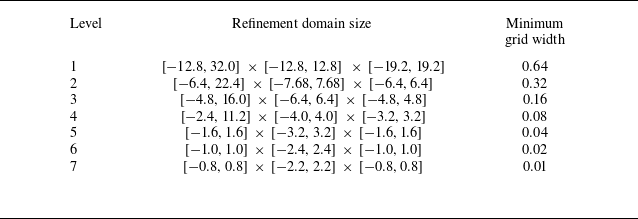
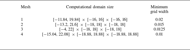
The validations of the numerical method and grid convergence are detailed in our previous works (Wang et al. Reference Wang, Zhang, He and Liu2013b , Reference Wang, He and Zhang2015a , Reference Wang, Zhang, He and Liub , Reference Wang, He and Liu2019; Zhang et al. Reference Zhang, He, Wang and Zhang2019; Tong, Yang & Wang Reference Tong, Yang and Wang2021; Chen, Liu & Wang Reference Chen, Liu and Wang2025). The mesh set-up has been tested in multiple bio-locomotion problems with similar wing geometry, wing kinematics and Reynolds number. With the time-dependent and time-averaged aerodynamic force coefficients adopted as convergence criteria, the present mesh resolution and computational domain size have ensured the convergence of the calculation. The aerodynamic force coefficients remain almost unchanged, whether the minimum grid width is reduced to half or the three edge lengths of the computational domain are all increased to 1.5 times and above (Wang et al. Reference Wang, He and Zhang2015a ; Chen et al. Reference Chen, Liu and Wang2025). Two examples of mesh convergence validation are provided in Appendix B.
We calculate the aerodynamic force coefficients of a unilateral local sweep morphing wing. The time-dependent lift coefficient and drag coefficient of the local sweep morphing wing are defined as follows:
 \begin{align} {{C}_{L}}\left ( t \right ) & =\frac {{{F}_{z}}\left ( t \right )}{{1}/{2}\;\rho U_{\textit{ref}}^{2}{{S}^b_{\textit{ref}}}}, \end{align}
 \begin{align} {{C}_{D}}\left ( t \right ) & =\frac {{{F}_{x}}\left ( t \right )}{{1}/{2}\;\rho U_{\textit{ref}}^{2}{{S}^b_{\textit{ref}}}}, \end{align}
where
 ${F}_{x}$
and
 ${F}_{z}$
are the aerodynamic force components in the streamwise and vertical directions, respectively. The reference velocity
 ${U}_{\textit{ref}}$
is the oncoming flow velocity
 ${U}_{\infty }$
, as mentioned previously. The reference area
 ${S}^b_{\textit{ref}}$
is the area
 $S^b_{w\textit{ing}}$
of a unilateral local sweep morphing wing. The constancy of this reference area is proven in Appendix A. The constant reference area enables the aerodynamic force coefficients to reflect the effects of the local sweep angles and ensures a fair comparison of total aerodynamic forces. The lift coefficient of the local sweep morphing wing is processed by a low-pass second-order Butterworth filter.
3. Results and discussion
In § 3.1, we examine the aerodynamic forces of the fixed wings with different local sweep angles. This investigation shows the advantages of this aerodynamic configuration and the significance of local sweep morphing. In § 3.2, the unsteady lift coefficient of the local sweep morphing in both forward and backward directions is analysed in terms of morphing kinematics, starts and durations. In § 3.3, the unsteady lift coefficient of the local sweep morphing is decomposed to reveal the contribution of the sweeping modification. In § 3.4, the sweeping-modification lift coefficient is modelled based on the extended lifting-line theory. In § 3.5, the asymmetry in sweeping-modification lift coefficient is elucidated through vortex dynamics caused by the vertical morphing velocity.
3.1. Aerodynamic forces of the fixed wings with different local sweep angles
Figure 3 presents the distribution of the average aerodynamic force coefficients of fixed wings with different local sweep angles. According to the signs of the sweep angles of the inner and outer wings, the fixed wings with different local sweep angles are categorised into four types of configurations, including: (i) the configuration with backward-swept inner and outer wings
 $({ \Lambda }_{\textit{iw}}\gt 0, { \Lambda }_{\textit{ow}}\gt 0)$
; (ii) the configuration with forward-swept inner wing and backward-swept outer wing
 $({ \Lambda }_{\textit{iw}}\lt 0, { \Lambda }_{\textit{ow}}\gt 0)$
; (iii) the configuration with forward-swept inner and outer wings
 $({ \Lambda }_{\textit{iw}}\lt 0, { \Lambda }_{\textit{ow}}\lt 0)$
; and (iv) the configuration with backward-swept inner wing and forward-swept outer wing
 $({ \Lambda }_{\textit{iw}}\gt 0, { \Lambda }_{\textit{ow}}\lt 0)$
, as illustrated in figure 3(a). These configurations are located in the four quadrant subspaces from I to IV, respectively. For each fixed-wing configuration, the aerodynamic force coefficients are averaged over one period of aerodynamic force oscillation when the flow reaches the fully developed unsteady separation state. The radial basis function is used to fit the distribution surface of the average aerodynamic force coefficients in figure 3(b–d). The dash-dotted line represents the configuration where the inner and outer wings have the same local sweep angle.
Average aerodynamic force coefficients in the space
 $({ \Lambda }_{\textit{iw}}, { \Lambda }_{\textit{ow}})$
spanned by the local sweep angles of the inner and outer wings. (a) Schematic diagram of the four typical fixed wings with different local sweep angles. (b) Average lift coefficient. (c) Average drag coefficient. (d) Average lift-to-drag ratio. In panel (a), red and blue represent backward-swept (positive) and forward-swept (negative) local sweep angles, respectively. In panels (b–d), square and circular symbols denote the maximum average lift configuration,
 $({ \Lambda }_{\textit{iw}}, { \Lambda }_{\textit{ow}})=(10^{\circ }, 30^{\circ })$
, and its symmetric configuration,
 $({ \Lambda }_{\textit{iw}}, { \Lambda }_{\textit{ow}})=(-10^{\circ }, -30^{\circ })$
, respectively.

The configurations with the same local sweep angle change the aerodynamic force to a limited extent. As the same sweep angle increases (towards backward direction), the average lift and drag coefficients first increase and then decrease. In contrast, the different local sweep angles enable the fixed wings to change the aerodynamic force significantly, thereby extending their aerodynamic performance. The average lift coefficient varies from 0.63 to 0.83 and the average drag coefficient varies from 0.57 to 0.71, while the average lift-to-drag ratio varies from 1.01 to 1.20. Their ranges normalised by corresponding maximum values are 0.24, 0.20 and 0.16, respectively. The configuration with a backward-swept inner wing is more advantageous for generating high lift, as shown in figure 3(b). Moreover, the configuration with a backward-swept outer wing is more conducive to attaining a high lift-to-drag ratio, as exhibited in figure 3(d). For the investigated gliding fixed wings with different local sweep angles, the maximum average lift configuration, the minimum average drag configuration and the maximum average lift-to-drag ratio configuration are all in Quadrant I. The corresponding combinations of the local sweep angles of the inner and outer wings are
 $(10^{\circ }, 30^{\circ })$
,
 $(20^{\circ }, 20^{\circ })$
and
 $(10^{\circ }, 20^{\circ })$
, respectively. Mind that the point
 $(20^{\circ }, 20^{\circ })$
representing the minimum average drag configuration is on the right boundary of display range in figure 3(c).
In gliding flight, a high geometric angle of attack causes the flow separation over the fixed wing. The separated flow exhibits unsteadiness due to the generation of the LEVs and TEVs that evolve at a characteristic frequency (Taira & Colonius Reference Taira and Colonius2009; Kim & Gharib Reference Kim and Gharib2010; DeVoria & Mohseni Reference DeVoria and Mohseni2017). This flow unsteadiness differs from that in flapping flight, where the characteristic frequency of the separated flow couples with that of the flapping motion to produce complex unsteady aerodynamic effects (Trizila et al. Reference Trizila, Kang, Aono, Shyy and Visbal2011; Chin & Lentink Reference Chin and Lentink2016). The fixed wings with different local sweep angles exhibit varying degrees of unsteadiness, which can be reflected by the dimensionless principal amplitude and frequency of the time-dependent lift coefficient, as shown in figure 4. The dimensionless principal amplitude and frequency are obtained through the Fourier transform of the time-dependent lift coefficient sequence within the dimensionless time range of 200–300. To reduce frequency leakage, the Hanning window function is employed to handle the series of the time-dependent lift coefficient. The dimensionless principal frequency is derived from normalisation by the characteristic frequency
 ${{U}_{\infty }}/{{\gamma }{c}_{\textit{max}}}$
.
Oscillation parameters of the time-dependent lift coefficient in the space
 $({ \Lambda }_{\textit{iw}}, { \Lambda }_{\textit{ow}})$
spanned by the local sweep angles of the inner and outer wings. (a) Dimensionless principal amplitude of the time-dependent lift coefficient. (b) Dimensionless principal frequency of the time-dependent lift coefficient. The square and circular symbols mark the maximum average lift configuration,
 $({ \Lambda }_{\textit{iw}}, { \Lambda }_{\textit{ow}})=(10^{\circ }, 30^{\circ })$
, and its symmetric configuration,
 $({ \Lambda }_{\textit{iw}}, { \Lambda }_{\textit{ow}})=(-10^{\circ }, -30^{\circ })$
, respectively.

The maximum average lift configuration exhibits the highest lift-coefficient amplitude of 0.11 and the highest lift-coefficient frequency of 0.38. The configurations with backward-swept inner wings (Quadrants I and IV) have higher amplitudes and frequencies of the lift coefficient compared with those with forward-swept inner wings (Quadrants II and III), indicating that the configurations with backward-swept inner wings enhance the unsteadiness. When the outer wing is also backward-swept, this unsteadiness is the most significant. The increased frequency of the backward-swept configurations relative to the unswept configurations is consistent with the experimental measurements of Huang & Lin (Reference Huang and Lin1995) and Yen & Hsu (Reference Yen and Hsu2007). On one hand, to enhance the average lift coefficient, configurations with backward-swept inner and outer wings are recommended. On the other hand, to reduce the lift coefficient oscillations, these same configurations should be avoided. This inherent trade-off means that the high average lift and low oscillating lift represent a contradiction in the gliding flight.
3.2. Unsteady lift of the local sweep morphing
We focus on the maximum average lift configuration,
 $({ \Lambda }_{\textit{iw}}, { \Lambda }_{\textit{ow}})=(10^{\circ }, 30^{\circ })$
, and its symmetric configuration with the local sweep angles of equal values, but opposite signs,
 $({ \Lambda }_{\textit{iw}}, { \Lambda }_{\textit{ow}})=(-10^{\circ }, -30^{\circ })$
. These two configurations are denoted by square and circular symbols, respectively, in figures 3 and 4. The average lift coefficients of the maximum average lift configuration and its symmetric configuration are 0.83 and 0.69, respectively. The time-dependent lift coefficient of the maximum average lift configuration has a dimensionless principal amplitude of 0.11 and a dimensionless principal frequency of 0.38. In contrast, that of the symmetric configuration has a dimensionless principal amplitude of 0.01 and a dimensionless principal frequency of 0.28.
The maximum average lift configuration generates a high average lift, while the symmetric configuration generates a low oscillating lift, representing two typical aerodynamic requirements. The local sweep morphing between the two configurations provides a solution to compromise the high average lift and low oscillating lift. The local sweep morphing in both the forward and backward directions can be achieved through actuations inspired by the shoulder and wrist of the avian wing, as shown in figure 5. Hereinafter, the pre-morphing wings of the forward and backward sweeping are consistently taken as the maximum average lift configuration and its symmetric counterpart, respectively.
Local sweep morphing between the maximum average lift configuration,
 $({ \Lambda }_{\textit{iw}}, { \Lambda }_{\textit{ow}})=(10^{\circ }, 30^{\circ })$
, and its symmetric configuration,
 $({ \Lambda }_{\textit{iw}}, { \Lambda }_{\textit{ow}})=(-10^{\circ }, -30^{\circ })$
: (a) forward sweeping; (b) backward sweeping. The solid and dashed outlines denote the configurations after and before morphing, respectively.

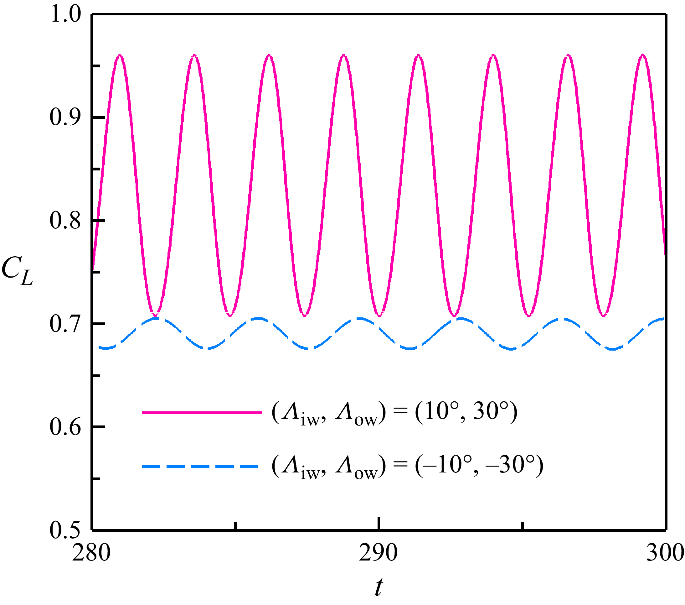
The controlled evolution of lift during the local sweep morphing is challenging, because the local sweep morphing initiates and terminates with distinct unsteady separated flows. Figure 6 illustrates that the fully developed lift coefficients undergo periodic oscillations with a single harmonic component, but with different amplitudes and frequencies. The oscillating lift coefficients, each with a principle frequency, correspond to the periodic unsteady type of Taira & Colonius (Reference Taira and Colonius2009), according to the given angle of attack of and aspect ratio. The Strouhal number, based on the principle frequency, projected chord length (
 ${{c}_{\textit{max}}}\sin \alpha$
) and free stream velocity, is 0.13 and 0.10 for the maximum average lift configuration and its symmetric configuration, respectively. These two values approach the converged Strouhal number of 0.12 from all periodic shedding cases under similar conditions. The maximum average lift configuration has a high dimensionless principal amplitude and a high dimensionless principal frequency, while the situation is the opposite for its symmetric configuration. The weak unsteadiness of the symmetric configuration may be related to the downwash effect of the tip vortices (Zhang & Taira Reference Zhang and Taira2022). The local sweep morphing requires to switch between two flows with such different unsteadiness.
Lift-coefficient history of two typical configurations to experience the local sweep morphing.

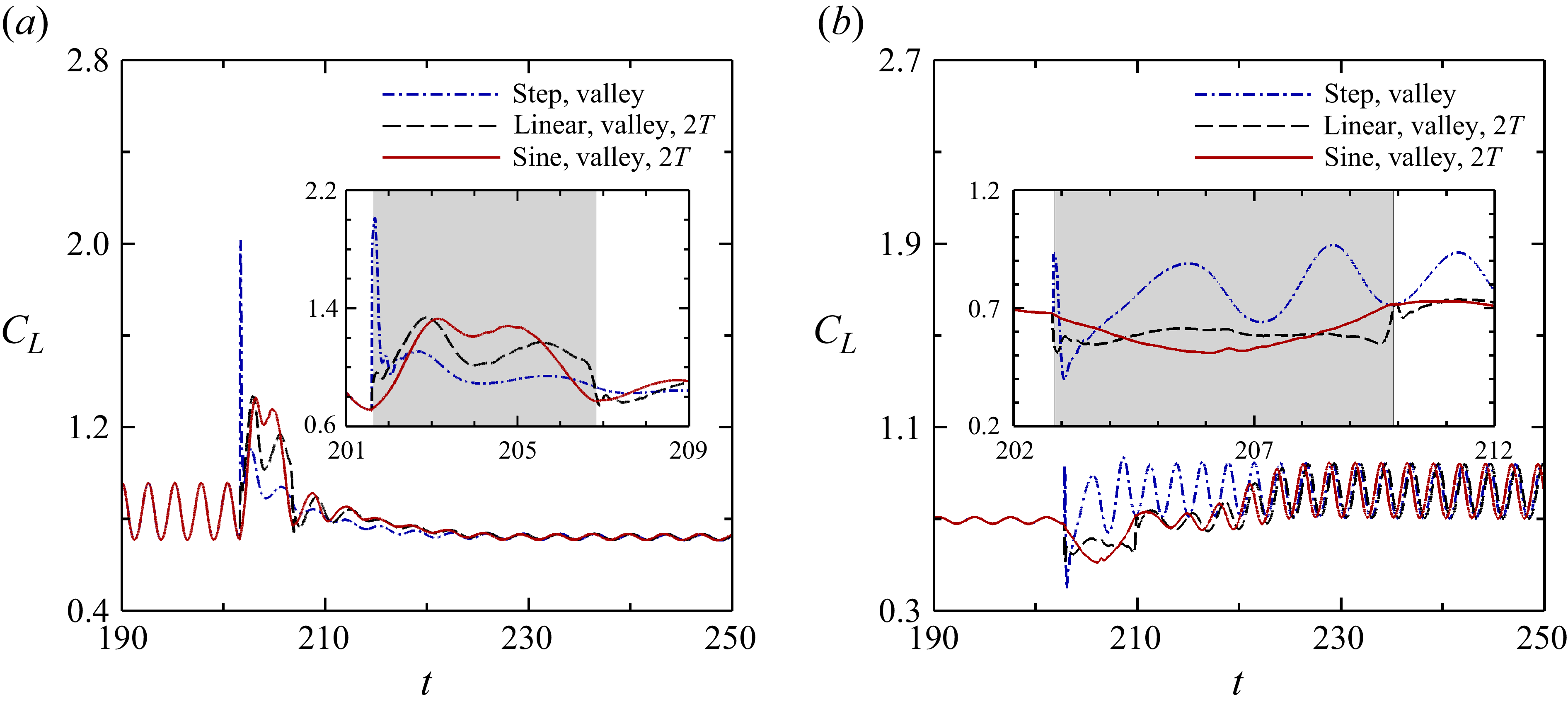
Figure 7(
a) displays the time-dependent lift coefficients during the forward sweeping under three morphing kinematics, with the morphing start of the valley moment and the morphing duration of twice the pre-morphing period (
 $T=2.60$
). The three morphing kinematics are in the step, linear and nonlinear sine forms, as shown in figure 2. The morphing phase
 $[{{t}_{0}},{{t}_{f}}]$
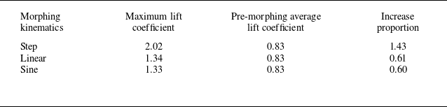
is magnified and highlighted by a shaded block. The lift characteristics of forward sweeping under the three morphing kinematics are summarised in Appendix C. For the step morphing kinematics, the lift coefficient experiences a steep change immediately after the morphing. Under the linear morphing kinematics, the lift coefficient also undergoes steep changes at the beginning and end of the morphing. These changes are notably reduced compared with those of step morphing. In contrast, the nonlinear sine morphing completely eliminates the steep change in the lift coefficient due to its smooth nature. However, the lift coefficient increases substantially during the morphing phase, leading to a lift overshoot. The local maximum lift coefficient increases by 60 % compared with the average lift coefficient of 0.83 before the morphing. The unsteady characteristics after the forward sweeping are the recurrence and decay of the lift peaks. This behaviour is similar to the lift coefficient response of the streamwise acceleration of the flat-plate wing under the same geometric angle of attack (Mulleners et al. Reference Mulleners, Mancini and Jones2017). It takes more than 10 convective time scales to reach the new unsteady state.
Effect of the morphing kinematics on the time-dependent lift coefficient: (a) forward sweeping; (b) backward sweeping.

The effect of morphing kinematics on the time-dependent lift coefficient during the backward morphing is shown in figure 7(
b). The same three morphing kinematics are applied with the morphing start of the valley moment and the morphing duration of twice the pre-morphing period (
 $T=3.52$
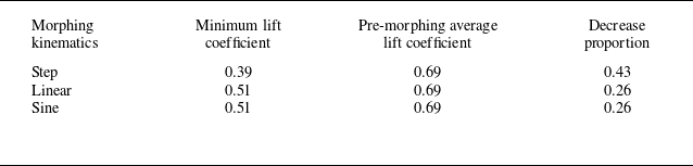
). The corresponding lift characteristics are presented in Appendix C. Compared with the forward sweeping, the lift coefficients of the step and linear morphing kinematics in the backward sweeping exhibit less steep changes. The lift coefficient of the nonlinear sine morphing decreases significantly during the morphing, resulting in a lift undershoot. The local minimum lift coefficient decreases by 27 % compared with the pre-morphing average lift coefficient of 0.69. The lift coefficient after the backward sweeping is characterised by the recurrence and growth of the lift peaks. Similarly, more than 10 convective time scales are required to arrive at the new unsteady state. The lift undershoot during the backward sweeping may cause the stall-like issues. The maximum lift undershoot has a smaller magnitude compared with the maximum lift overshoot. This difference arises from the combined effects of the sweeping direction and pre-morphing unsteadiness.
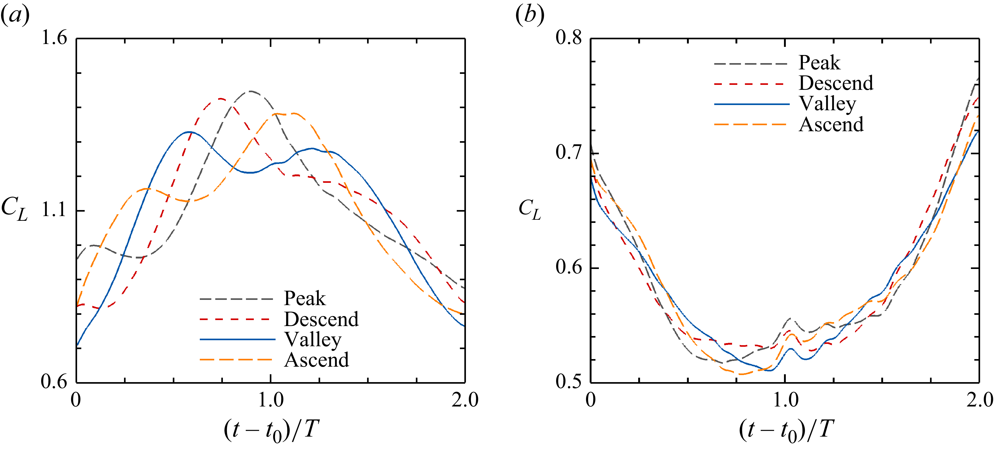
The lift over/undershoot is expected to be alleviated by adjusting the morphing start and duration. Figure 8 illustrates the effect of the morphing start on the time-dependent lift coefficient. The nonlinear sine morphing kinematics is adopted and the morphing duration is fixed at twice the pre-morphing period. Four typical morphing starts including the peak (
 ${t}_{p}$
), descending-mean (
 ${t}_{d}$
), valley (
 ${t}_{v}$
) and ascending-mean (
 ${t}_{a}$
) moments are compared. We take the morphing start of the valley moment as the reference. To align the morphing phase, we use the scaled time relative to the morphing start,
 $(t-t_{0})/T$
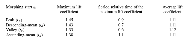
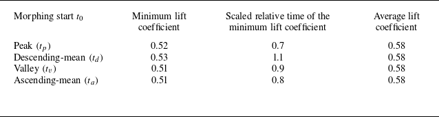
, here referred to as scaled relative time. The comparison in Appendix C shows that starting at the valley moment can achieve the most pronounced reduction in the maximum lift overshoot during the forward sweeping. In contrast, adjusting the morphing start cannot effectively reduce the lift undershoot during the backward sweeping, due to the weak unsteadiness present before this sweeping.
Effect of the morphing start on the time-dependent lift coefficient: (a) forward sweeping; (b) backward sweeping. The nonlinear sine morphing kinematics is employed with the morphing duration of
 $2T$
and the morphing starts of the peak (
 $t_p$
), descending-mean (
 $t_d$
), valley (
 $t_v$
) and ascending-mean (
 $t_a$
) moments. The morphing phase is aligned using the scaled relative time.

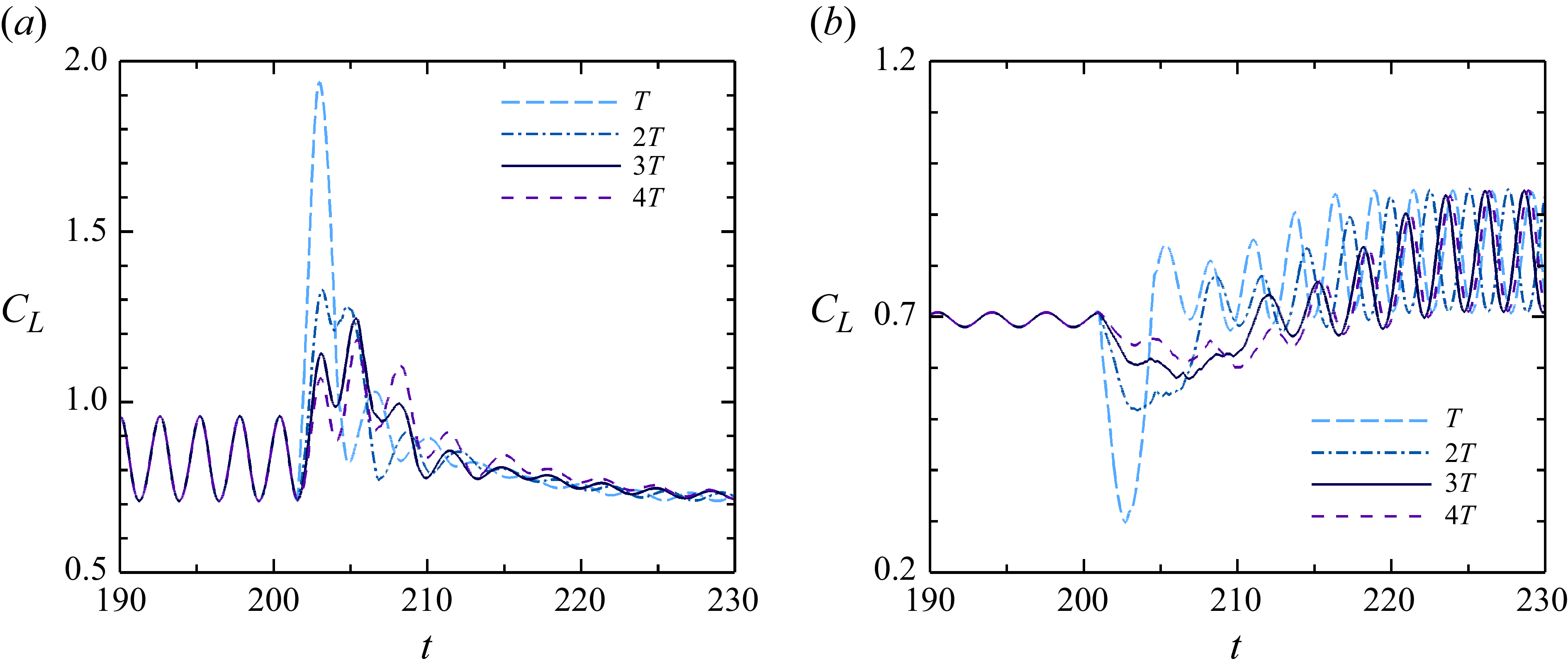
Figure 9 presents the time-dependent lift coefficients under different morphing durations. With the same nonlinear sine morphing kinematics, the forward and backward sweeping wings start morphing from the valley and peak moments, respectively. Four typical morphing durations spanning from one to four times the pre-morphing lift coefficient period
 $T$
are compared. We use the morphing duration of
 $2T$
as the reference. For the forward sweeping in figure 9(
a), when the morphing duration is shortened from
 $2T$
to
 $T$
, the maximum lift coefficient arises significantly, giving rise to a severe lift overshoot. When the morphing duration is prolonged from
 $2T$
to
 $3T$
or
 $4T$
, the maximum lift coefficient experiences a decrease. The lift characteristics during the forward sweeping are also observed in the accelerating start of the flat-plate wing (Mancini et al. Reference Mancini, Manar, Granlund, Ol and Jones2015; Stevens et al. Reference Stevens2017). Similarly, during the backward sweeping in figure 9(
b), shortening the morphing duration increases the lift undershoot, while prolonging the morphing duration decreases the lift undershoot.
Effect of the morphing duration on the time-dependent lift coefficient: (a) forward sweeping; (b) backward sweeping. The nonlinear sine morphing kinematics is employed with the morphing start of the valley (
 $t_v$
) and peak (
 $t_p$
) moments for the forward and backward sweeping cases, respectively. The morphing durations ranging from
 $T$
to
 $4T$
are adopted.

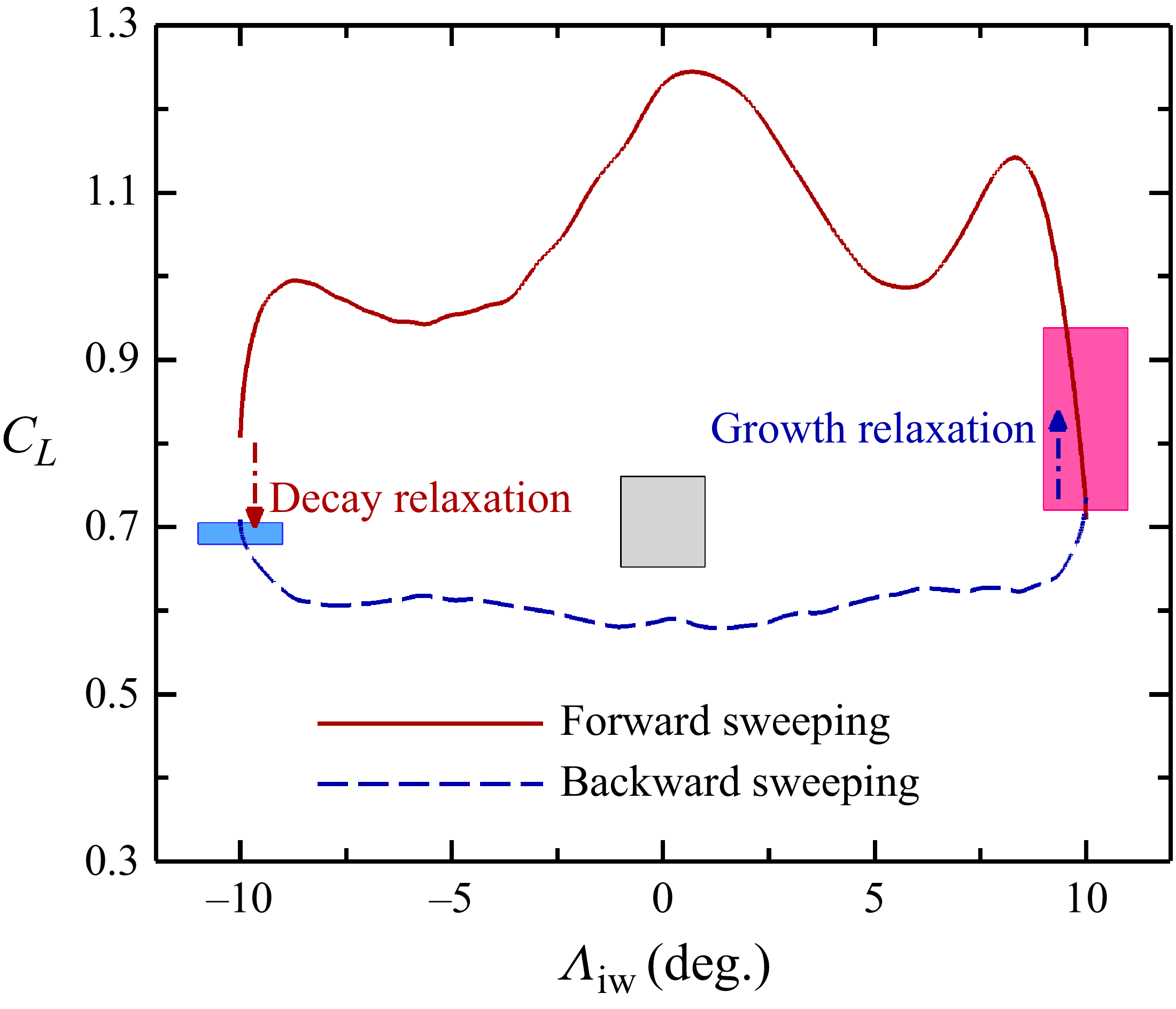
Figure 10 plots the lift-coefficient hysteresis loop of a favourable local sweep morphing. The favourable morphing strategy is achieved using the nonlinear sine kinematics with the morphing start of the valley moment and the morphing duration of
 $3T$
during the forward sweeping, and the same kinematics with the morphing start of the peak moment during the backward sweeping. The lift-coefficient branches of the forward sweeping and the backward sweeping are denoted by the red solid and blue dashed lines, respectively. The morphing process is indicated by the local sweep angle
 ${ \Lambda }_{\textit{iw}}$
of the inner wing. To clarify the difference of the lift coefficient between the sweeping wing (dynamic) and fixed-wing (static) cases, the oscillating ranges of three fixed-wings are represented by the rectangle columns. The left and right columns denote the pre-morphing fixed-wings of backward sweeping (
 ${{ \Lambda }_{\textit{iw}}}=-10{}^\circ$
,
 ${{ \Lambda }_{\textit{ow}}}=-30{}^\circ$
) and forward sweeping (
 ${ \Lambda }_{\textit{iw}}=10{}^\circ$
,
 ${{ \Lambda }_{\textit{ow}}}=30{}^\circ$
), respectively. The middle column corresponds to the unswept fixed-wing, a configuration traversed during the morphing process.
Hysteresis loop of the lift coefficient under the favourable local sweep morphing. Red solid line (forward sweeping): the nonlinear sine kinematics with the morphing start of the valley moment
 $t_v$
and the morphing duration of
 $3T$
. Blue dashed line (backward sweeping): the nonlinear sine morphing kinematics with the morphing start of the peak moment
 $t_p$
and the morphing duration of
 $3T$
. The top and bottom of the rectangle column display the maximum and minimum lift coefficients, respectively, of the fixed wing with variable local sweep angles. From left to right, the local sweep angles
 $({ \Lambda }_{\textit{iw}}, { \Lambda }_{\textit{ow}})$
are
 $(-10^{\circ }, -30^{\circ })$
,
 $(0^{\circ }, 0^{\circ })$
and
 $(10^{\circ }, 30^{\circ })$
.

As shown in figure 10, the lift coefficient of the forward sweeping is higher than that of the backward sweeping during the local sweep morphing. The lift oscillation of the forward sweeping is stronger than that of the backward sweeping, which is a continuation of the highly unsteady initial flow. After the forward sweeping, a relaxation time of lift decay (denoted by the downward red arrow) is required to return to the fully developed state. Conversely, a growth relaxation (denoted by the upward blue arrow) occurs after the backward sweeping. These characteristics are distinct from those of the sweep morphing at the low geometric angles of attack, which aligns with the steady initial flow (Zeng et al. Reference Zeng, Liu, Shao and Li2023; Bai et al. Reference Bai, Yang, Guo, Xiao, Liu and Deng2025). Furthermore, the mentioned differences in the time-dependent lifts of the forward and backward sweeping cases are caused by the hysteresis nature of the flow. The lift hysteresis of the morphing wing is owing to the fact that the flow cannot immediately respond to the changes in the morphing motion of the wing, which is similar to the pitching situation (Mittal & Saxena Reference Mittal and Saxena2002).
3.3. Sweeping modification of the lift over/undershoot
The time-dependent lift coefficient during the local sweep morphing, especially the lift over/undershoot, depends on the pre-morphing flow state. Furthermore, the lift coefficient profiles under the forward-sweeping and no-morphing cases exhibit similar shapes, both featuring two peaks, although their magnitudes are different, as displayed in figure 11( a). This similarity implies that one component of the lift coefficient during the morphing is extended from the pre-morphing lift coefficient. When the extended lift coefficient is subtracted from the total lift coefficient during the morphing, the net lift coefficient attributes to the modification from the local sweep morphing, as shown in figure 11( b). We refer to the net component as the sweeping-modification lift coefficient.
Decomposition of the time-dependent lift coefficient during the forward sweeping: (a) lift coefficients under the forward sweeping and no sweeping; (b) sweeping-modification lift coefficient. The forward-sweeping morphing phase is visualised by the shaded block. The negligible shift from zero at the morphing start results from the filtering of the lift coefficient.

Figure 12 presents the dependence of the sweeping-modification lift coefficient on the morphing start. The sweeping-modification lift coefficient is plotted against the scaled relative time. For the forward sweeping, the sweeping-modification lift coefficients exhibit similar convex profiles under different morphing starts, as shown in figure 12( a). In the first 30 % of the morphing phase, the sweeping-modification lift coefficients almost overlap, indicating an interval in which the sweeping-modification lift coefficient is independent of the morphing start. Mancini et al. (Reference Mancini, Manar, Granlund, Ol and Jones2015) also report the similarity in the measured lift coefficients during the accelerating start of a flat-plate wing. They find that the circulatory lift component is not affected by the acceleration profile in the first 40 % of the accelerating phase. In the remaining part of the forward sweeping, deviations occur in the sweeping-modification lift coefficients. For the backward sweeping, the sweeping-modification lift coefficients under different morphing starts have a consistent concave profile and overlap throughout the morphing phase, as displayed in figure 12( b). The similarity of the sweeping-modification lift coefficients facilitates the modelling of the time-dependent lift over/undershoot from the local sweep morphing.
Effect of the morphing start on the sweeping-modification lift coefficient: (a) forward sweeping; (b) backward sweeping. The vertical dashed line represents the mid-moment of the morphing phase.

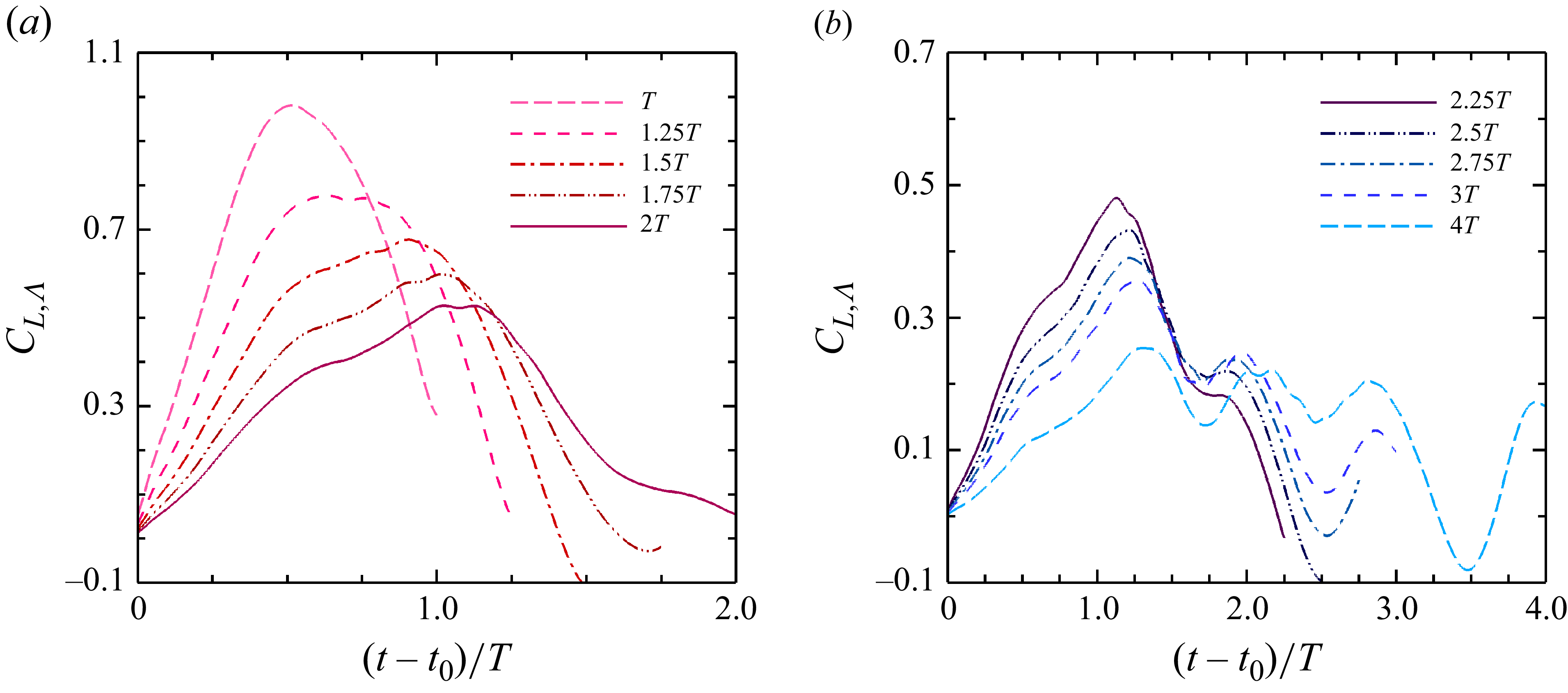
Figure 13 illustrates the effect of the morphing duration on the sweep-modification lift coefficient during the forward sweeping. Two sweeping modes are distinguished by the morphing duration of
 $2T$
. A fast sweeping mode corresponds to the morphing duration
 ${{t}_{f}}-{{t}_{0}}\in [T, 2T]$
, while a slow sweeping mode corresponds to the morphing duration
 ${{t}_{f}}-{{t}_{0}}\in (2T, 4T]$
. For the fast sweeping mode in figure 13(
a), the sweeping-modification lift coefficient almost reaches its peak value at mid-moment of the morphing phase. Before and after this peak value, the sweeping-modification lift coefficient shows a monotonic ascent and a monotonic descent, respectively. As the morphing duration increases from
 $T$
to
 $2T$
, the growth of the lift coefficient in the ascending stage and its decay in the descending stage both slow down, but with different rates. The profile of the sweeping-modification lift coefficient changes from a near-symmetric shape to an asymmetric one. As will be explained later, the asymmetric profile consists of a symmetric basic component and an asymmetric variation, which correlate with the horizontal and vertical components of the morphing velocity, respectively.
Effect of the morphing duration on the sweeping-modification lift coefficient during the forward sweeping: (a) fast sweeping mode with the morphing duration
 ${{t}_{f}}-{{t}_{0}}\in [T, 2T]$
; (b) slow sweeping mode with the morphing duration
 ${{t}_{f}}-{{t}_{0}}\in (2T, 4T]$
.

By contrast, the slow sweeping mode is characterised by a new extreme value on the descending branch of the sweeping-modification lift coefficient (see figure 13
b). As the morphing duration increases, this lift extreme develops into a secondary lift peak. When the morphing duration reaches
 $4T$
, several successive lift peaks appear in the descending stage due to the relaxation from the slow deceleration. From a decomposition perspective, the fast sweeping mode reflects a mechanism that constitutes the framework of the sweeping-modification lift coefficient, while the slow sweeping mode adjusts its descending branch by introducing additional unsteady effects.
Figure 14 presents the change in the maximum magnitude of the sweeping-modification lift coefficient with the morphing duration. There is a nonlinear decrease in the maximum sweeping-modification lift coefficient
 ${C}_{L, \Lambda , max }$
during the forward sweeping, as shown in figure 14(
a). The maximum sweeping-modification lift coefficient decreases fast under the fast sweeping mode with the morphing duration
 ${{t}_{f}}-{{t}_{0}}\in [T, 2T]$
, while it decreases slowly under the slow sweeping mode with the morphing duration
 ${{t}_{f}}-{{t}_{0}}\in (2T, 4T]$
. Similarly, the minimum sweeping-modification lift coefficient
 ${C}_{L, \Lambda , min }$
during the backward sweeping exhibits a nonlinear increase with different increase rates under the fast and slow sweeping modes. The nonlinear changes follow the negative power laws,
 \begin{align} {{C}_{L, \Lambda , max }} & ={{C}_{ \Lambda -}}{{\left ( \frac {t_f-{{t}_{0}}}{T} \right )}^{-1}}, \\[-12pt]\nonumber \end{align}
 \begin{align} {{C}_{L, \Lambda , min }} & ={{C}_{ \Lambda +}}{{\left ( \frac {t_f-{{t}_{0}}}{T} \right )}^{-1}}, \end{align}
Effect of the morphing duration on the maximum magnitude of the sweeping-modification lift coefficient. (a) Maximum sweeping-modification lift coefficient during the forward sweeping. (b) Minimum sweeping-modification lift coefficient during the backward sweeping. The circular symbols denote the results of numerical simulations, while the solid lines represent the fitted negative power laws.

where
 ${C}_{ \Lambda -}=1.0$
and
 ${C}_{ \Lambda +}=-0.4$
, measuring the change rates of the maximum and minimum sweeping-modification lift coefficients, respectively.
Through the maximum and minimum sweeping-modification lift coefficients, the sweeping-modification lift coefficients under the forward and backward sweeping cases are both scaled to the interval of
 $[0,1]$
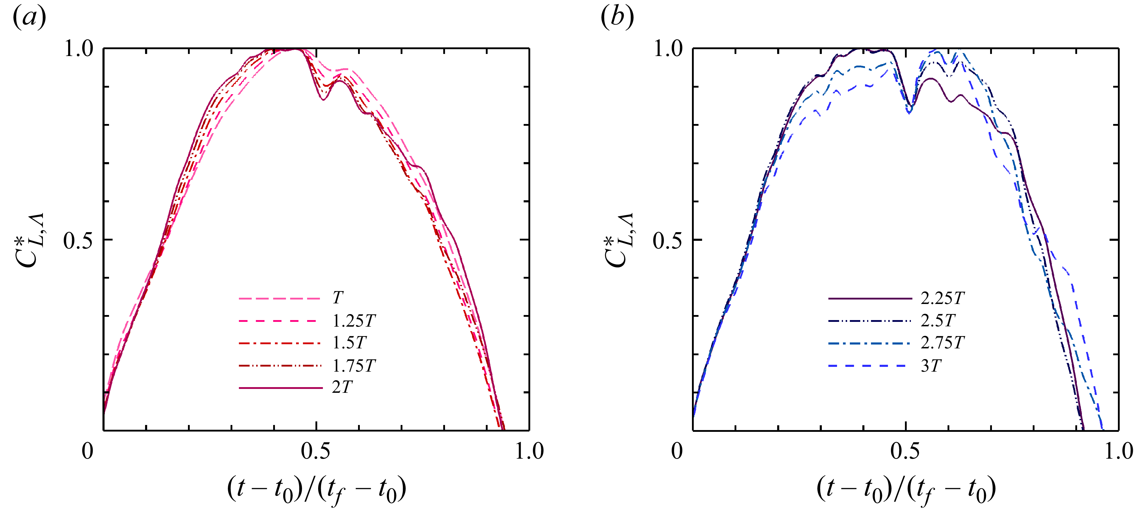
. As shown in figure 15, for the forward sweeping, the scaled sweeping-modification lift coefficients,
 $C_{L, \Lambda }^{*}={{{C}_{L, \Lambda }}}/{{{C}_{L, \Lambda , max }}}$
, exhibit similarity among different morphing durations, especially within the ascending stage,
 ${ ( t-{{t}_{0}} )}/{ ( {{t}_{f}}-{{t}_{0}} )}\in [ 0,0.5 ]$
. The lift coefficient during the descending stage shows different divergences between the fast and slow sweeping modes. Higher similarity of the scaled sweeping-modification lift coefficients is found during the backward sweeping, as displayed in Appendix D. The similarity of the scaled sweeping-modification lift coefficients under different morphing durations paves the way for the modelling of time-dependent lift over/undershoot from local sweep morphing.
Scaled sweeping-modification lift coefficients under different forward sweeping durations: (a) fast sweeping mode; (b) slow sweeping mode.

3.4. Reduced-order unsteady lift model for the local sweep morphing
3.4.1. Kinematic model of the local sweep morphing wing
As the foundation for modelling the lift over/undershoot, it is essential to propose a kinematic model of the local sweep morphing wing. We define the straight-line segment connecting the two points of the wing root and the wing tip on the half-chord line as the effective half-chord line, as shown in figure 16. For the wing with the inner-wing sweep angle
 ${ \Lambda }_{\textit{iw}}$
and the outer-wing sweep angle
 ${ \Lambda }_{\textit{ow}}$
, the effective sweep angle
 ${ \Lambda }_{e}$
is defined here as the angle between the effective half-chord line and the spanwise axis (Anderson Reference Anderson2010), and is expressed as
 \begin{equation} {{ \Lambda }_{e}}={{\tan }^{-1}}\left ( \frac {\tan {{ \Lambda }_{\textit{i}w}}+\tan {{ \Lambda }_{\textit{ow}}}}{2} \right ). \end{equation}
The local sweep angles
 $({{ \Lambda }_{\textit{iw}}},{{ \Lambda }_{\textit{ow}}})$
of the maximum average lift configuration are
 $(10^{\circ },30^{\circ })$
, leading to its effective sweep angle of
 ${21}^{\circ }$
. The corresponding symmetric configuration has the effective sweep angle with equal magnitudes and opposite signs.
Schematic diagram of the kinematical model of the local sweep morphing wing: (a) three-dimensional view; (b) in-plane view; (c) left side view.

The nonlinear sine morphing kinematics in terms of the effective sweep angle is
 \begin{equation} {{ \Lambda }_{e}}(t)=\frac {{{ \Lambda }_{e,f}}-{{ \Lambda }_{e,0}}}{2}\sin \left [ \frac {\pi }{{{t}_{f}}-{{t}_{0}}}t-\frac {\pi \left ( {{t}_{f}}+{{t}_{0}} \right )}{2\left ( {{t}_{f}}-{{t}_{0}} \right )} \right ]+\frac {{{ \Lambda }_{e,f}}+{{ \Lambda }_{e,0}}}{2}, \end{equation}
where
 ${ \Lambda }_{e,0}$
and
 ${ \Lambda }_{e,f}$
are the initial and final effective sweep angles, respectively. For the forward sweeping,
 ${{ \Lambda }_{e,0}}={21}^{\circ }$
and
 ${{ \Lambda }_{e,f}}=-{21}^{\circ }$
.
The time derivative of the effective sweep angle is
 \begin{equation} \frac {\textrm{d}{{ \Lambda }_{e}}(t)}{\textrm{d}t}=\frac {{{ \Lambda }_{e,f}}-{{ \Lambda }_{e,0}}}{2}\cos \left [ \frac {\pi }{{{t}_{f}}-{{t}_{0}}}t-\frac {\pi \left ( {{t}_{f}}+{{t}_{0}} \right )}{2\left ( {{t}_{f}}-{{t}_{0}} \right )} \right ] \frac {\pi }{{{t}_{f}}-{{t}_{0}}}. \end{equation}
With the effective sweep angle, the sweep morphing in the shearing way results in the effective tangential displacement
 $\Delta {{s}_{e}}$
at a spanwise position
 $y$
(
 $0 \leqslant {y} \leqslant {b}_{\textit{iw}}+{b}_{\textit{ow}}$
) as follows:
 \begin{equation} \Delta {s_e} (t) = y\left [ \tan {{ \Lambda }_{e}}\left ( t \right )-\tan {{ \Lambda }_{e}}\left ( {{t}_{0}} \right ) \right ], \quad {{t}_{0}}\leqslant t\leqslant {{t}_{f}}. \end{equation}
According to the definition of the effective tangential displacement, the sweep morphing velocity
 ${U}_{s}$
at the spanwise position
 $y$
is
 \begin{equation} {U}_{s}\left ( t \right )={\frac {{U}_{\infty }y}{{\gamma }{c}_{\textit{max}}}}\frac {1}{{{\cos }^{2}}\left [ {{ \Lambda }_{e}}\left ( t \right ) \right ]}\frac {\textrm{d}{{ \Lambda }_{e}}\left ( t \right )}{\textrm{d}t}. \end{equation}
The net forward-flight velocity of the wing section at the spanwise position
 $y$
is
 \begin{equation} {{U}_{x}}\left ( t \right )={{U}_{\infty }}-{{U}_{s}}\left ( t \right )\cos \alpha. \end{equation}
The normal component of the net forward-flight velocity (see figure 17) perpendicular to the effective half-chord line is
 \begin{equation} {{U}_{n}}\left ( t \right )={{U}_{x}}\left ( t \right )\cos {{ \Lambda }_{e}}\left ( t \right ). \end{equation}
Normal component of the net forward-flight velocity changes with the morphing duration: (a) forward sweeping; (b) backward sweeping. The vertical axis range of panel (a) is twice that of panel (b).

Here, the spanwise position
 $y$
is selected at the wing tip, namely,
 $y={b}_{\textit{iw}}+{b}_{\textit{ow}}$
. This is because the wing tip typically serves as the characteristic spanwise position to measure the unsteady effects of bio-locomotion (Taylor, Nudds & Thomas Reference Taylor, Nudds and Thomas2003).
3.4.2. Lift model of the local sweep morphing wing
We start to develop a reduced-order lift model for local sweep morphing wings, which facilitates low-cost lift evaluation during their conceptual design and feedback control (Brunton et al. Reference Brunton, Rowley and Williams2013). Previously, Manar & Jones (Reference Manar and Jones2019) extend the classical thin aerofoil theory to the cases of high geometric angles of attack and variable translational velocities, and obtain a reduced-order unsteady model for predicting the lift coefficient of a linearly accelerating flat-plate wing. However, this model is shown to overestimate the local overshoot of the normal force on the flat plate. To take into account the effects of a finite wingspan, we adopt the same assumptions to extend Prandtl’s lifting-line theory and propose a time-dependent lift model for a three-dimensional wing with the variable translational velocity. The detailed derivation of this model is presented in Appendix E.
The lift-curve slope of the proposed model is
 \begin{equation} {{\kappa }_{3\text{-}\textrm{D}}}=\frac {{{\kappa }_{{2\text{-}\textrm{D}}}}}{E+\displaystyle \frac {{{\kappa }_{{2\text{-}\textrm{D}}}}}{\pi {AR}}{{\left ( \frac {{{U}_{\textit{ref}}}}{{{U}_{w\textit{ing}}}} \right )}^{2}}\left ( 1+\delta \right )}, \end{equation}
where
 ${\kappa }_{{2\text{-}\textrm{D}}}$
is the lift-curve slope of a two-dimensional flat-plate aerofoil,
 $E$
is the edge velocity correction factor,
 $ AR$
is the aspect ratio of the unilateral wing (see Appendix A),
 ${U}_{w\textit{ing}}$
is the translational velocity of the forward-flight wing, and
 ${U}_{\textit{ref}}$
is the reference velocity for defining the lift coefficient in (2.8) and (2.9). Here,
 $\delta$
is the Glauert correction factor for the induced angle of attack, which accounts for the effects of a non-elliptical circulation distribution. The proposed model (3.10) indicates that the translational velocity affects the lift coefficient in the form of kinetic energy.
In this work, the two-dimensional lift-curve slope
 ${\kappa }_{{2\text{-}\textrm{D}}}$
is given as 5.16 to account for the Reynolds number effect (Okamoto, Yasuda & Azuma Reference Okamoto, Yasuda and Azuma1996; Nabawy & Crowther Reference Nabawy and Crowther2014). The edge velocity correction factor and Glauert correction factor are formulated to incorporate the effect of the sweep angle. With reference to the treatment of Polhamus (Reference Polhamus1949), the edge velocity correction factor
 ${E}_{ \Lambda }$
of the wing with a sweep angle
 $ \Lambda$
can be obtained by comparing the correction equations of Jones (Reference Jones1941) and Küchemann (Reference Küchemann1952), that is,
 \begin{equation} {{E}_{ \Lambda }}=\sqrt {\frac {1}{{{\cos }^{2}} \Lambda }+{{\left ( \frac {{{\kappa }_{{2\text{-}\textrm{D}}}}}{\pi {{AR}}} \right )}^{2}}}. \end{equation}
The Glauert correction factor
 ${\delta }_{ \Lambda }$
for the wing with a sweep angle
 $ \Lambda$
is determined according to the theoretical data of DeYoung (Reference DeYoung1947). Due to the differences in the Reynolds number and aspect ratio, the data of lift-curve slope are corrected using the relation by Gutierrez-Castillo et al. (Reference Gutierrez-Castillo, Aguilar-Cabello, Alcalde-Morales, Parras and del Pino2021), expressed as
 \begin{equation} {{\kappa}_{3\text{-}\textrm{D}}} \propto {{\left ( 1+\frac {{{10}^{6}}}{{Re}} \right )}^{-\sigma }}\left [ \sqrt {1+{{\left ( \frac {\lambda }{\pi {{AR}}} \right )}^{2}}}+\frac {\lambda }{\pi {{AR}}} \right ]^{-1}, \end{equation}
where the parameter
 $\lambda$
is set to its original value of 3.79. The increase rate
 $\sigma$
is decreased slightly to
 $1/6$
, since the sensitivity of the lift coefficient reduces at high Reynolds number (Quinn Jr Reference Quinn1945). The corrected lift-curve slope corresponds to the Reynolds number of
 $O(10^4)$
, which is the minimum order of magnitude allowed by the relation (3.12). The Glauert correction factor is calculated by substituting the corrected lift-curve slope into (3.10) that involves (3.11) and excludes the translational velocity of the wing. The dependence of the Glauert correction factor on the sweep angle
 $ \Lambda$
is approximated by
 \begin{equation} {\delta }_{ \Lambda } = {C_{\delta 1}} \left ( \frac {\pi }{180}{ \Lambda }-{C_{\delta 2}} \right )^2 + {C_{\delta 3}}, \end{equation}
where the constant parameters are taken as
 ${C_{\delta 1}}=0.13$
,
 ${C_{\delta 2}}=0.08$
and
 ${C_{\delta 3}}=0.17$
. This fitted formula coincides with the data for the sweep angles ranging from
 $-30^\circ$
to
 $30^\circ$
.
For the local sweep morphing wing, the sweep angle
 $ \Lambda$
in (3.11) and (3.13) is the effective sweep angle
 ${ \Lambda }_{e}$
, and the translational velocity
 ${U}_{w\textit{ing}}$
of the wing is the normal component
 ${U}_{n}$
of the net forward-flight velocity perpendicular to the effective half-chord line, as expressed in (3.9). Substituting (3.9), (3.11) and (3.13) into the model (3.10) yields the lift-curve slope formula applicable to the swept wing,
 \begin{equation} {{\kappa }_{{3\text{-}\textrm{D}}, \Lambda }}=\frac {{{\kappa }_{{2\text{-}\textrm{D}}}}}{\displaystyle {{E}_{ \Lambda }}+\frac {{{\kappa }_{{2\text{-}\textrm{D}}}}}{{\pi} {{AR}}}{{\left ( \frac {{{U}_{\infty }}}{{{U}_{n}}} \right )}^{2}} \left ( 1+{\delta }_{ \Lambda } \right )}. \end{equation}
The lift coefficient at high geometric angles of attack can be derived from that at low geometric angles of attack for the unsteady flows dominated by the LEVs (Nabawy & Crowther Reference Nabawy and Crowther2014; Wang et al. Reference Wang, Goosen and van Keulen2016), as detailed in Appendix F. We follow this approach of constructing the lift model at high geometric angles of attack and obtain the lift coefficient of the swept wing with variable translational velocity,
 \begin{equation} {{{\hat C}^{\prime}}_{L, \Lambda }} = \frac {1}{2} \frac {{{\kappa }_{{2\text{-}\textrm{D}}}}}{\displaystyle {E}_{ \Lambda }+\frac {{{\kappa }_{{2\text{-}\textrm{D}}}}}{{\pi} {{AR}}}{{\left ( \frac {{{U}_{\infty }}}{{{U}_{n}}} \right )}^{2}} \left ( 1+{\delta }_{ \Lambda } \right )} \sin \left ( 2\alpha \right ). \end{equation}
Here and hereinafter, the interim lift coefficient evaluated by the different lifting-line models is marked with a hat symbol to distinguish it from the final one.
To capture the key unsteady effects of the vortical flow, an unsteady Kutta–Joukowski theorem (Gennaretti & Giansante Reference Gennaretti and Giansante2022; Giansante, Bernardini & Gennaretti Reference Giansante, Bernardini and Gennaretti2024; Frassoldati et al. Reference Frassoldati, Giansante, Bernardini and Gennaretti2024) is incorporated into the current theoretical framework, as presented in Appendix G. Through the transformation and simplification of a frequency response function correlating the sectional lift and circulation, the unsteady Kutta–Joukowski theorem can be explicitly represented in the unsteady formulation of the model (3.15),
 \begin{equation} {{{\hat C}^{\prime \prime}}_{L, \Lambda }}( {t} )=\frac {1}{2}\frac {{{\kappa }_{{2\text{-}\textrm{D}}}}}{\displaystyle {{E}_{ \Lambda }}\left ( {t} \right )+\frac {{{\kappa }_{{2\text{-}\textrm{D}}}}}{{\pi} {{AR}}}{{\left [ \frac {{{U}_{\infty }}}{{{U}_{n}}\left ( {t} \right )} \right ]}^{2}} \frac {1+{\delta }_{ \Lambda }(t)}{{\varPhi }(t)}}\sin \left ( 2\alpha \right ), \end{equation}
where
 $\varPhi$
is an unsteady indicator function, which quantifies the wake memory effect associated with the unsteady evolution and interaction of vortex structures.
In this work, (3.16) is intended for two purposes. One is to construct a model for predicting the lift over/undershoot induced by the local sweep morphing and the other is to quantify the unsteady effects of local sweep morphing. For the unsteady flow dominated by a single principal frequency, the unsteady indicator function takes the specific form of
 \begin{equation} {\varPhi }_{k_T}(t) \simeq {C}_{k_T} =\sqrt {1+k^2_T}, \end{equation}
where
 $k_T$
is a reduced frequency, expressed as
 \begin{equation} k_T=\frac {\pi {{c}_{\textit{max}}^{*}}}{T{{U}_{\infty }^{*}}}, \end{equation}
where the quantities with an asterisk as the superscript are non-dimensionalised. The principal frequency (
 $1/T$
) of the pre-morphing lift coefficient is adopted, since the lift over/undershoot during the local sweep morphing is closely related to the pre-morphing unsteadiness of the flow, as shown in § 3.2.
It is noticed that the unsteady Kutta–Joukowski theorem (G8) reduces to the steady theorem multiplied by a constant scale factor
 ${C}_{k_T}$
. We would like to point out that it is appropriate to close the lift model through the steady theorem, when the unsteady effects induced by the local sweep morphing are sufficiently weak. In this sense, the reduced form
 ${C}_{k_T}$
of the unsteady indicator function measures the relevant unsteady effects based on the principal frequency. It corrects the steady Kutta–Joukowski theorem to the unsteady counterpart by taking the time derivative of the sectional circulation into account, as explained in Appendix G. The steady Kutta–Joukowski theorem is recovered when the unsteady indicator function
 ${C}_{k_T}=1$
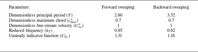
. Numerical values for calculating the unsteady indicator function
 ${C}_{k_T}$
are shown in table 3. The unsteady indicator function
 ${C}_{k_T}$
equals 1.31 for the forward sweeping and 1.18 for the backward sweeping. The increases of 31 % and 18 % in the unsteady indicator function for the forward and backward sweeping cases, respectively, indicate that the unsteady theorem reflects non-negligible unsteady effects as compared with the steady theorem. Additionally, the unsteady indicator function
 ${C}_{k_T}$
in terms of the reduced frequency
 $k_T$
captures the discrepancies in lift generation associated with the pre-morphing flow states between the forward and backward sweeping cases. We would like to note that the reduced form
 ${C}_{k_T}$
is not permitted for flows characterised by multiple-frequencies, being applicable exclusively to the single-frequency scenario. Although a certain phase difference between sectional lift and circulation is induced at the values of the reduced frequency (Gennaretti & Giansante Reference Gennaretti and Giansante2022), we consider only the magnitude effects for the purposes of the present application, as stated in Appendix G.
Numerical values employed to calculate the unsteady indicator function.

Through excluding the change in the lift coefficients of the fixed wings with different local sweep angles before morphing, the evaluated sweeping-modification lift coefficient is written as
 \begin{equation} {{\hat C}_{L, \Lambda }}\left ( {t} \right )={{{\hat C}^{\prime \prime}}_{L, \Lambda }}\left ( {t} \right )-{{{\hat C}^{\prime \prime}}_{L, \Lambda }}\left ( t_0 \right ), \end{equation}
where the excluded initial lift coefficient
 ${{\hat C}^{\prime \prime}}_{L, \Lambda } ( t_0 )$
is
 \begin{aligned} {{\hat C}^{\prime \prime}}_{L, \Lambda } (t_0) &= \frac {1}{2} \frac {{{\kappa }_{{2\text{-}\textrm{D}}}}}{\displaystyle {{E}_{ \Lambda }}(t_0)+\frac {{{\kappa }_{{2\text{-}\textrm{D}}}}}{{\pi} {{AR}}}{{ \left [ \frac {{{U}_{\infty }}}{{{U}_{n}}(t_0)} \right ]}^{2}} \left [\frac {1+{\delta }_{ \Lambda }(t_0)}{\sqrt {1+k_T^2}}\right ]} \sin (2 \alpha ) \\ &= \frac {1}{2} \frac {{{\kappa }_{{2\text{-}\textrm{D}}}}}{\displaystyle {\sqrt {\frac {1}{{{\cos }^{2}} \Lambda _{e,0}}+{{\left ( \frac {{{\kappa }_{{2\text{-}\textrm{D}}}}}{{\pi} {{AR}}} \right )}^{2}}}}+\frac {{{\kappa }_{2{\text{-}\textrm{D}}}}}{{\pi} {{AR}}}{{ \left [ \frac {{{U}_{\infty }}}{{{{U}_{x}}\left ( t_0 \right )\cos {{ \Lambda }_{e,0}}}} \right ]}^{2}}\left [\frac {1+{\delta }_{ \Lambda }(t_0)}{\sqrt {1+k_T^2}}\right ]} \sin (2 \alpha ) \\ &= \frac {1}{2} \frac {{{\kappa }_{{2\text{-}\textrm{D}}}}\;{{\cos }^{2}}{{ \Lambda }_{e,0}}}{\displaystyle {{\cos }^{2}}{{ \Lambda }_{e,0}}\sqrt {\frac {1}{{{\cos }^{2}}{{ \Lambda }_{e,0}}}+{{\left ( \frac {{{\kappa }_{{2\text{-}\textrm{D}}}}}{{\pi} {{AR}}} \right )}^{2}}}+\frac {{{\kappa }_{{2\text{-}\textrm{D}}}}}{{\pi} {{AR}}}\left [\frac {1+{C_{\delta 1}} \left ( { \Lambda }_{e,0}-{C_{\delta 2}} \right )^2 + {C_{\delta 3}}}{\sqrt {1+k_T^2}}\right ]} \sin \left ( 2\alpha \right ). \end{aligned}
In this derivation, the relation
 ${{U}_{x}}(t_0)={U}_{\infty }$
is applied.
Dividing the evaluated sweeping-modification lift coefficient (3.19) by its maximum, we get the evaluated scaled sweeping-modification lift coefficient
 \begin{equation} {\hat C}_{L, \Lambda }^{*}\left ( t \right )=\frac {{{\hat C}_{L, \Lambda }}\left ( t \right )}{{{\hat C}_{L, \Lambda , {max}}}}. \end{equation}
Similarly, in the backward sweeping, the evaluated scaled sweeping-modification lift coefficient is
 \begin{equation} {\hat C}_{L, \Lambda }^{*}\left ( t \right )=\frac {{{\hat C}_{L, \Lambda }}\left ( t \right )}{{{\hat C}_{L, \Lambda , {min}}}}. \end{equation}
As shown in figure 18, the evaluated scaled sweeping-modification lift coefficient reflects the changes in the normal velocity components
 $U_n$
in figure 17, especially the symmetry around the mid-moment. This symmetry originates from the horizontal component of the morphing velocity,
 $U_{s}\cos \alpha$
. The symmetric component forms the basis of the sweeping-modification lift coefficient. Moreover, the evaluated scaled sweeping-modification lift coefficients under the forward and backward sweeping cases exhibit consistent trends to their numerical counterparts in figures 15 and 28. For the forward sweeping, the theoretical model captures the similarity of the numerical results during the ascending stage,
 ${ ( t-{{t}_{0}} )}/{ ( {{t}_{f}}-{{t}_{0}} )}\in [ 0,0.5 ]$
. For the backward sweeping, it also predicts an increase when
 ${ ( t-{{t}_{0}} )}/{ ( {{t}_{f}}-{{t}_{0}} )}\in [ 0.15,0.45 ]$
and a decrease near the mid-moment as the morphing duration is prolonged. These consistencies indicate that
 \begin{equation} {\hat C}_{L, \Lambda }^{*} = { C}_{L, \Lambda }^{*} \end{equation}
or
 \begin{equation} \frac {{{\hat C}_{L, \Lambda }}\left ( t \right )}{{{\hat C}_{L, \Lambda , {max/min}}}}= \frac {{{C}_{L, \Lambda }}\left ( t \right )}{{{C}_{L, \Lambda , {max/min}}}}. \end{equation}
Here, the consistent similarity results between the numerical simulation and theoretical model provide a means for further correcting the magnitude of the maximum lift over/undershoot. With the consistent similarity, the lift model is augmented by including the viscous effects associated with flow separation. The possible underestimation in lift due to additional nonlinearity of the lift curve in the pre-stall regions (Hewes Reference Hewes1978) can be compensated for.
Scaled sweeping-modification lift coefficient evaluated with the proposed model: (a) forward sweeping; (b) backward sweeping.

From (3.24), the sweeping-modification lift coefficient is formulated as
 \begin{equation} {{{C}_{L, \Lambda }}\left ( t \right )} = {{{\hat C}_{L, \Lambda }}\left ( t \right )}\; \frac {{{C}_{L, \Lambda , {max/min}}}}{{{\hat C}_{L, \Lambda , {max/min}}}}. \end{equation}
This expression, along with (3.1), (3.2) and (3.16)–(3.20), constitutes the reduced-order unsteady model for the lift over/undershoot from the local sweep morphing, which can be used to evaluate the total lift coefficient during the morphing by adding the pre-morphing lift coefficient.
The proposed lift model is reduced-order since it captures the essential dynamics in lift generation during the local sweep morphing with a relatively small number of physical factors (Lucia, Beran & Silva Reference Lucia, Beran and Silva2004; Karbasian & Vermeire Reference Karbasian and Vermeire2022). The model provides quantitatively accurate characterisations of the local sweep morphing dynamics at a computational cost substantially lower than that of the original numerical model, while offering an accessible framework for readily interpreting the underlying dynamics. In this model, the dominant factors considered are the horizontal morphing velocity, non-elliptic circulation distribution and spanwise flow induced by the local sweep angles, high geometric angle of attack and unsteady wake memory effect.
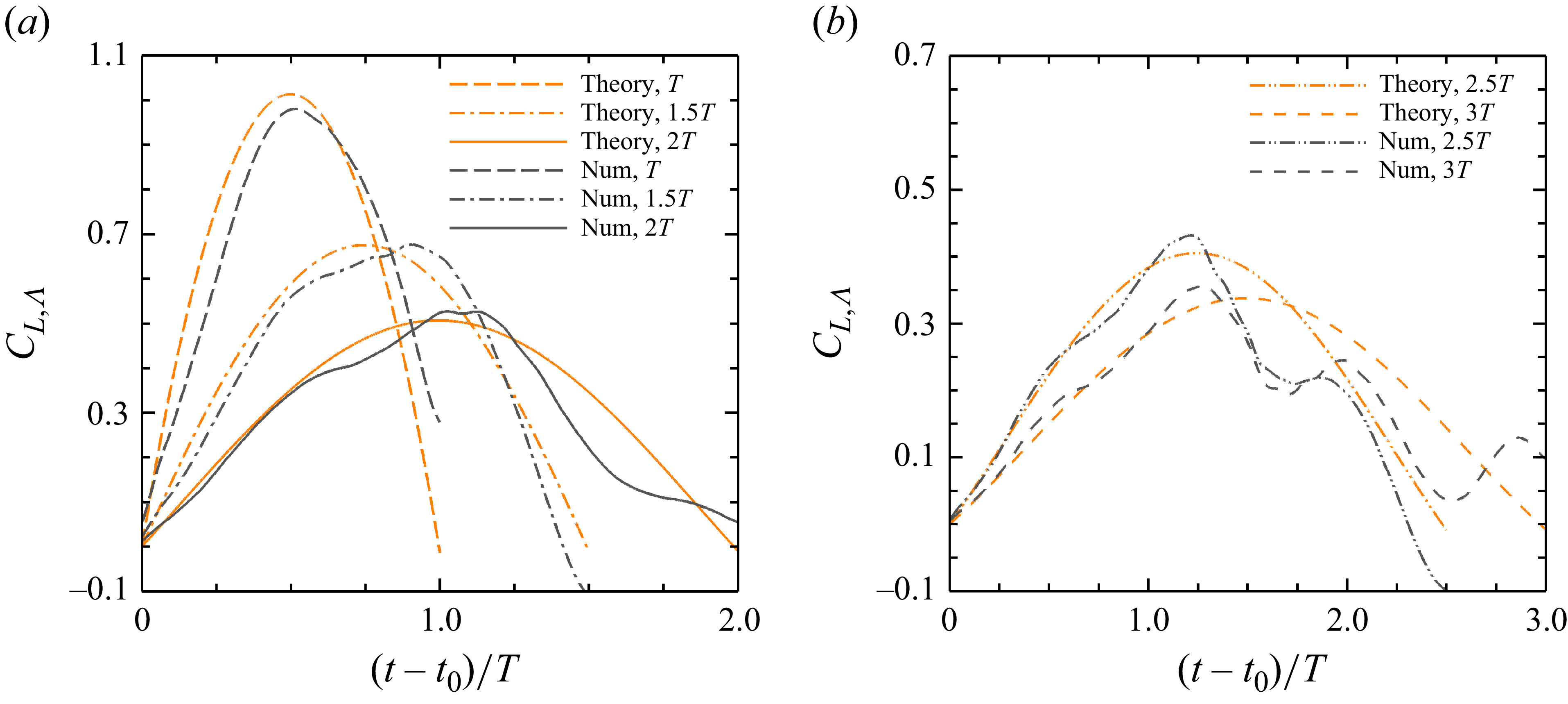
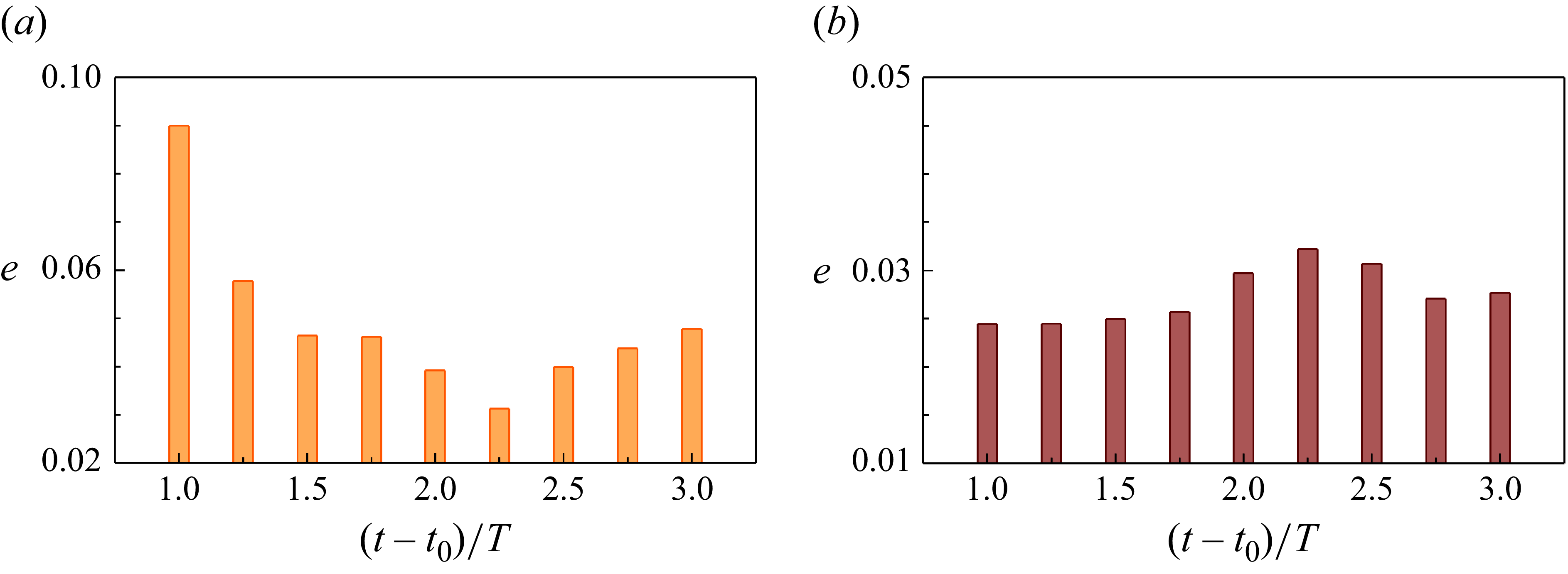
Figure 19 presents the prediction of the reduced-order unsteady model and the result of the numerical simulation for the sweeping-modification lift coefficient when the change in the morphing start is considered. The numerical result is the average sweeping-modification lift coefficient under the four typical morphing starts and the same morphing duration of
 $2T$
. The theoretical prediction is in reasonable agreement with the numerical result. In figure 19(a), the reduced-order unsteady model predicts the increase in the sweeping-modification lift coefficient during the accelerating stage
 $ ( t - {{t}_{0}} )/T\in [ 0,1 ]$
of the forward sweeping (that is, the ascending stage of the sweeping-modification lift coefficient). Nevertheless, the reduced-order unsteady model underestimates the maximum value of the sweeping-modification lift coefficient. Compared with the prediction of the reduced-order unsteady model, the numerical results are characterised by an earlier timing of the maximum sweeping-modification lift coefficient and a rapid decay after the maximum value, which determine the primary and secondary peaks of the total lift coefficient, respectively. The prediction for backward sweeping is similar to that for forward sweeping, as shown in figure 19(b). The difference between the theoretical and numerical sweeping-modification lift coefficients arises from the additional unsteady effects caused by the local sweep morphing. These unsteady effects lead to the asymmetry in the profile of the sweeping-modification lift coefficient during the ascending stage
 $ ( t - {{t}_{0}} )/T\in [ 0,1 ]$
and descending stage
 $ ( t - {{t}_{0}} )/T\in [ 1,2 ]$
.
Comparison between the theoretical prediction and the numerical simulation for the sweeping-modification lift coefficient when the morphing start changes: (a) forward sweeping; (b) backward sweeping. The solid line corresponds to the theoretical model, while the dashed line represents the average value of the numerical results under the four typical morphing starts in figure 12.

Figures 20 and 21 show the comparison between the reduced-order unsteady model and the numerical simulation for the sweeping-modification lift coefficients under the morphing durations of
 $T$
,
 $1.5T$
,
 $2T$
,
 $2.5T$
and
 $3T$
. The morphing start is fixed at the valley moment for the forward sweeping and the peak moment for the backward sweeping. Overall, the predictions of the reduced-order unsteady model present a good alignment with the numerical results, although there are apparent deviations in the slow sweeping mode. The prediction error is measured by the time-averaged absolute value of the difference between the theoretical and numerical sweeping-modification lift coefficients, that is,
 \begin{equation} e=\frac {1}{{{t}_{f}}-{{t}_{0}}}\int _{{{t}_{0}}}^{{{t}_{f}}}{\left | C_{L, \Lambda }^{({theory})}\left ( t \right )-C_{L, \Lambda }^{({num})}\left ( t \right ) \right |}\,{\textrm{d}}t. \end{equation}
Comparison between the theoretical prediction and the numerical simulation for the sweeping-modification lift coefficient of the forward sweeping when the morphing duration changes: (a) fast sweeping mode; (b) slow sweeping mode. The solid lines correspond to the theoretical model, while the dashed lines represent numerical results.

Comparison between the theoretical prediction and the numerical simulation for the sweeping-modification lift coefficient of the backward sweeping when the morphing duration changes: (a) fast sweeping mode; (b) slow sweeping mode. The solid lines correspond to the theoretical model, while the dashed lines represent numerical results.

For the forward sweeping cases, the prediction error of the model is almost less than 0.06, except for the maximum error of 0.09 observed at the morphing duration of
 $T$
, as exhibited in figure 22(
a). The prediction error for backward sweeping cases is relatively uniform, with a maximum error of only approximately 0.03, which corresponds to the morphing duration of
 $2.25T$
, as shown in figure 22(
b). Discrepancies in the sweeping-modification lift coefficient emerge during the deceleration stage under the fast morphing mode and increase under the slow morphing mode. At longer morphing durations, the low horizontal morphing velocity weakens the role of this factor, including the associated higher-order unsteady effects, and brings out other inherent higher-order unsteady effects in the flow.
Error between the theoretical prediction and the numerical simulation for the sweeping-modification lift coefficient across different morphing durations: (a) forward sweeping; (b) backward sweeping.

The contribution of unsteady effects attributed to the local sweep morphing can be quantified through the numerical results and theoretical formula (3.16). The unsteady effects comprise low-order components, characterised by (3.17), and higher-order components. Rearranging the expression (3.16) yields
 \begin{equation} \varPhi \left ( t \right )=\frac {1+{{\delta }_{ \Lambda }}\left ( t \right )}{\displaystyle \frac {\pi AR}{{{\kappa }_{\text{2-}\textrm{D}}}}\left [ \frac {{{\kappa }_{\text{2-}\textrm{D}}}\sin \left ( 2\alpha \right )}{2{{{{C}^{\prime \prime}}}_{L, \Lambda }}\left ( t \right )}-{{E}_{ \Lambda }}\left ( t \right ) \right ]{{\left [ \frac {{{U}_{n}}\left ( t \right )}{{{U}_{\infty }}} \right ]}^{2}}}. \end{equation}
A sweeping indicator can be defined in an analogous way to the sweeping-modification lift coefficient. The lift coefficient induced by local sweep morphing and extended pre-morphing lift coefficient are substituted into (3.27) to obtain the corresponding unsteady indicator functions
 $\varPhi$
. Their difference
 $\Delta \varPhi$
is first time-averaged and its absolute value is then taken to ensure positive values under the backward sweeping cases. The sweeping indicator is formulated as
 \begin{equation} {{\varPhi }_{ \Lambda }}=\frac {1}{{{t}_{f}}-{{t}_{0}}}\left | \int _{{{t}_{0}}}^{{{t}_{f}}}{\Delta \varPhi \left ( t \right )}\;{ }{\textrm d}t \right |, \end{equation}
which measures the intensity of the unsteady effects associated with the horizontal morphing velocity.
In the slow mode of forward sweeping, the sweep indicator
 ${\varPhi }_{ \Lambda }$
decreases with the morphing duration, as shown in figure 23. This indicates that a reduction in the horizontal morphing velocity is accompanied by weaker higher-order unsteady effects associated with it. For the backward sweeping, the sweep indicator
 ${\varPhi }_{ \Lambda }$
exhibits almost no change with the morphing duration (remaining around 0.014), which reflects that the higher-order unsteady effects associated with the horizontal morphing velocity are insensitive to the morphing duration. At the morphing duration of
 $4T$
, the sweeping indicators for the forward sweeping and backward sweeping cases reach a near-identical level.
Sweeping indicator across different morphing durations. The square symbol represents the forward sweeping, while the diamond symbol denotes the backward sweeping.

Moreover, the added-mass lift component is neglectable in the modelling because the adopted wing model has zero thickness and its local sweep morphing is limited to the wing plane. For an accelerating elliptic aerofoil immersed in a constant free stream, Limacher (Reference Limacher2021) decomposes the total added-mass force into a chordwise component
 ${{F}_{a,\shortparallel }}=- ( {\pi }/{4}\; )\rho h^{2}a_{\shortparallel }$
and a chord-normal component
 ${{F}_{a,\bot }}=- ( {\pi }/{4}\; )\rho c^{2}a_{\bot }$
, where
 $h$
denotes aerofoil thickness (minor axis length),
 $c$
denotes aerofoil chord (major axis length),
 $a_{\shortparallel }$
is the chordwise acceleration component and
 $a_{\bot }$
is the chord-normal acceleration component. In this work, the conditions of the zero thickness wing and the in-plane morphing are equivalent to
 $h=0$
and
 $a_{\bot }=0$
, respectively. Thus, both the two added-mass force components vanish. This estimation still holds when three-dimensional effects are considered (Brennen Reference Brennen1982; Manar & Jones Reference Manar and Jones2019). Even for wing accelerations where the translating direction forms a large angle with the wing plane, the added-mass lift component accounts for only a small fraction of the total lift in both fast and slow modes (Mancini et al. Reference Mancini, Manar, Granlund, Ol and Jones2015).
3.5. Vortex dynamics of the local sweep morphing
The asymmetry in the sweeping-modification lift coefficient profile correlates with the vortex dynamics of the local sweep morphing. This correlation is revealed by examining how the local sweep morphing modifies the vortex dynamics of the pre-morphing configuration.
Before the forward sweeping, the maximum average lift coefficient configuration generates the highly unsteady flow, which is characterised by the alternating formation, growth and shedding of the LEVs and TEVs. Figure 24 displays the instantaneous vortex structures at two typical moments corresponding to the lift peak and the lift valley. The vortex structures of the maximum average lift coefficient configuration are identified using the
 $Q$
-criterion. The isosurfaces of
 $Q=2.5$
are plotted and coloured by the normalised spanwise vorticity
 ${\omega }_y$
. The distribution of the spanwise vorticity within a slice at the spanwise position
 ${y}/({b}_{\textit{iw}}+{b}_{\textit{ow}})=37\,\%$
is presented in the right-hand side of each panel. The slice is represented by the solid black line on the wing surface in the left-hand side. As the lift coefficient ascends and approaches its peak, the streamwise size of the LEVs grows continuously. Concurrently, the TEVs are convected downstream until they shed. At the moment of the lift peak, the streamwise size of the LEVs is close to the local chord length of the wing section, as shown in figure 24(a). The LEVs upstream interact with the detached TEVs downstream, producing a downwash flow between them. In the subsequent descending of lift coefficient, new TEVs start to form and the spiral structure of the LEVs is broken. At the moment of the lift valley, the TEVs upstream interact with the detached LEVs downstream, inducing an upwash flow between them, as shown in figure 24(b). The near-field vorticity carries significant weight in the lift generation of the fixed-wing, as demonstrated in the force decomposition theory (Chang Reference Chang1992; Chang, Yang & Chu Reference Chang, Yang and Chu2008). In the wing section, the near-wake is dominated only by the large-scale LEVs and TEVs, without smaller-scale secondary vortices. Consequently, the lift coefficients exhibits no high-frequency components in figure 6.
Instantaneous vortices of the maximum average lift coefficient configuration: (a) moment of the lift peak; (b) moment of the lift valley. In the left-hand side of each panel, the vortex structures of the fixed wing with different local sweep angles are identified using the isosurfaces of
 $Q = 2.5$
and coloured by the normalised spanwise vorticity
 ${\omega }_y$
. The right-hand side shows the spanwise vorticity within a slice at the spanwise position
 ${y}/({b}_{\textit{iw}}+{b}_{\textit{ow}})=37\,\%$
, which is indicated by the solid black line on the wing surface in the left-hand side.

To explain the asymmetry of the sweeping-modification lift coefficient profile, we select the mid-moments,
 ${(t-{{t}_{0}})}/{T}=0.5$
and
 ${(t-{{t}_{0}})}/{T}=1.5$
, of the forward-sweeping acceleration and deceleration stages in figure 25, corresponding to the two peak values (see figure 11
a) of the extended pre-morphing lift coefficient, respectively. At these two moments, the relative streamwise position between the LEVs and TEVs is consistent with that at the peak moments of the pre-morphing lift coefficient. That is, the LEVs are located upstream of the detached TEVs. However, the normal distances of the LEVs from the upper surface of the wing are different. This is closely related to the change in the vertical velocity component,
 ${{U}_{s}}\sin \alpha$
(see figure 16), caused by the local sweep morphing. When the vertical morphing velocity increases, the LEVs approach the upper wing surface. Conversely, when the vertical morphing velocity decreases, the LEVs move farther from the upper wing surface. The vertical morphing velocity changes the interaction between the LEVs and the upper wing surface, leading to the asymmetric profile of the sweeping-modification lift coefficient.
Instantaneous vortices of the morphing wing during the forward sweeping: (a) mid-moment
 ${(t-{{t}_{0}})}/{T}=0.5$
of the acceleration stage; (b) mid-moment
 ${(t-{{t}_{0}})}/{T}=1.5$
of the deceleration stage. The forward sweeping is characterised by the nonlinear sine morphing kinematics with the morphing start of the valley moment (
 $t_v$
) and the morphing duration of
 $2T$
. In the left-hand side of each panel, the vortex structures of the local sweeping wing are identified using the isosurfaces of
 $Q = 2.5$
and coloured by the normalised spanwise vorticity
 ${\omega }_y$
. The slice in the right-hand side has the same spanwise position as that in figure 24.

Figure 9 shows that at the morphing durations of
 $3T$
and
 $4T$
, the second lift peak becomes larger than the first, which is different from the trend observed at shorter morphing duration of
 $2T$
. This phenomenon is related to the vortex formation and interaction modulated by the horizontal morphing velocity. The decomposition of the lift coefficient facilitates the extraction of key vortex dynamics. The sweeping-modification lift coefficient reflects the vortex dynamics associated with the horizontal morphing velocity. The symmetric component of the sweeping-modification lift coefficient reaches its maximum at the mid-moment of the morphing phase. For the morphing duration of
 $3T$
, the second one among the three peaks of the extended pre-morphing lift coefficient during the morphing phase aligns with the peak of the sweeping-modification lift coefficient. It is obvious that the second lift peak becomes the largest after superimposition. For the morphing duration of
 $4T$
, the extended pre-morphing lift coefficient exhibits two peaks respectively before and after the mid-moment. Since the second lift peak is located in the acceleration phase with the vortex lift advantage (as detailed previously) and is closer to the moment of maximum horizontal morphing velocity than the first peak, it generates the highest lift.
4. Conclusions
The lift response to the local sweep morphing of an avian-inspired gliding wing under the fully developed unsteady separated flow state is investigated in this work. The time-dependent lift coefficient and the dynamic vortex structures are acquired by numerically solving the Navier–Stokes equations. The effects of the morphing kinematics, start and duration during the local sweep morphing in both the forward and backward directions are elucidated.
The fixed wing with different local sweep angles can enhance the average lift coefficient and lift-to-drag ratio. The configuration with the backward-swept inner and outer wings creates the maximum average lift coefficient. However, this configuration also maximises the frequency and amplitude of the time-dependent lift coefficient. The incompatibility between high average and low oscillating lift coefficients necessitates the local sweep morphing. During the forward sweeping from the configuration with the maximum average lift coefficient to its symmetric counterpart featuring the low oscillating lift coefficient, the lift coefficient shows a prominent maximum overshoot. Conversely, during the opposite backward sweeping, the lift coefficient exhibits a remarkable maximum undershoot. Following the lift over/undershoot transient, the lift coefficient converges to a new unsteady separated state after the decay or growth of successive lift peaks.
It is found that the smooth nonlinear morphing kinematics eliminates the steeple change in the lift coefficient at the velocity discontinuities compared with the step and linear morphing kinematics. The morphing start at the lift extrema opposing the over/undershoot direction (e.g. lift valleys for overshoot) is shown to reduce the lift over/undershoot when the pre-morphing lift coefficient exhibits high frequency and amplitude. Additionally, elongating the morphing duration enables a significant reduction in the lift over/undershoot.
The time-dependent lift coefficient during the morphing is decomposed into the extended pre-morphing lift coefficient and the sweeping-modification lift coefficient, which account for the contributions of constant-velocity translating and variable-velocity sweeping, respectively. Based on Prandtl’s lifting-line theory, we derive a lift model for the finite wing with variable translational velocity. Furthermore, we propose a reduced-order unsteady model for the sweeping-modification lift coefficient of the local sweep morphing wing. The proposed model predicts the symmetry sweeping-modification lift coefficient, dominated by the horizontal morphing velocity. The asymmetry in the sweeping-modification lift coefficient is related to the modulation of the unsteady interaction between the leading-edge vortices and the upper wing surface through the vertical morphing velocity. This work sheds light on the surging flow of the wing, which could assist the aerodynamic design of the bio-inspired multifunctional aircraft.
To enhance the accuracy and robustness of the proposed model, the effects of Reynolds number, large-scale separation and spanwise flow need to be further quantified. We will examine the specific issues that were not adequately addressed in subsequent studies.
Acknowledgements
We would like to thank the reviewers for their insightful comments and constructive suggestions, which have improved the quality and rigour of this paper.
Funding
We sincerely appreciate financial support from the National Natural Science Foundation of China (NSFC) the Excellence Research Group Program for multiscale problems in nonlinear mechanics (Grant No. 12588201). This work is also supported by the National Natural Science Foundation of China (Grant No. 12425207), the Chinese Academy of Sciences Project for Young Scientists in Basic Research (Grant No. YSBR-087).
Declaration of interests
The authors report no conflict of interest.
Data availability statement
The data that support the findings of this work are available from the corresponding author upon reasonable request.
Appendix A. Details of the wing geometry
The geometry of the local sweep morphing wing is detailed in this appendix. As illustrated in figure 26(
a), the outline of the wing model is the closed curve
 $P_1P_3P_6P_9P_{11}P_7P_4P_1$
and its half-chord line is the polyline
 $P_2P_5P_{11}$
. The inner wing is the parallelogram
 $P_1P_3P_6P_4$
, with its half-chord line being line segment
 $P_2P_5$
. The outer wing consists of the parallelogram
 $P_4P_6P_9P_7$
and the semi-ellipse
 $P_7P_9P_{11}$
. The centre of this semi-ellipse is the midpoint
 $P_8$
of the line segment
 $P_7P_9$
. The centrally symmetric counterpart of the semi-ellipse
 $P_7P_9P_{11}$
is denoted by a dashed curve. The semi-ellipse
 $P_7P_9P_{11}$
is inscribed in the parallelogram
 $P_7P_9P_{12}P_{10}$
. The points of tangency are the point
 $P_7$
on the line
 $P_4P_{10}$
, point
 $P_9$
on the line
 $P_6P_{12}$
and point
 $P_{11}$
on the line
 $P_{10}P_{12}$
. The ellipse to which the semi-ellipse
 $P_7P_9P_{11}$
belongs is the maximum-area ellipse inscribed in the parallelogram, when the points of tangency are the midpoints of the respective edges, as shown in figure 26(
b). According to the properties of the maximum-area inscribed ellipse, the line segment
 $P_5P_{11}$
is the half-chord line of the outer wing.
Geometry of the local sweep morphing wing: (a) definition of wing geometry; (b) ellipse of maximum area inscribed in a parallelogram.

The inner wing has a fixed semi-span
 ${b}_{\textit{iw}}$
(spanwise distance between the lines
 $P_1P_3$
and
 $P_4P_6$
) and a uniform chord length
 ${c}_{\textit{max}}$
. The area of the inner wing is
 ${S}_{1} = {b}_{\textit{iw}}{c}_{\textit{max}}$
. The outer wing also has a fixed semi-span
 ${b}_{\textit{ow}}$
(spanwise distance between the lines
 $P_4P_6$
and
 $P_{10}P_{12}$
). Within this semi-span, the parallelogram part occupies
 $\beta {b}_{\textit{ow}}$
(spanwise distance between the lines
 $P_4P_6$
and
 $P_7P_9$
), while the semi-elliptical part occupies
 $(1-\beta ) {b}_{\textit{ow}}$
(spanwise distance between the lines
 $P_7P_9$
and
 $P_{10}P_{12}$
), where the partition factor
 $\beta = 0.15$
. The chord of the parallelogram part is uniformly specified as
 ${c}_{\textit{max}}$
, while that of the semi-elliptical part decreases towards the wing tip. The area of the parallelogram part is
 ${S}_{2} = \beta {b}_{\textit{ow}}{c}_{\textit{max}}$
. For a general ellipse inscribed in a parallelogram, its area is
 \begin{equation} {S}_{\textit{ellipse}}({l}_{t})=\frac {1}{2}\pi {{l}_{h}}\sqrt {\left ( {{l}_{b}}-{{l}_{t}} \right ){{l}_{t}}}, \end{equation}
where
 ${l}_{h}$
and
 ${l}_{b}$
are the height and base of the parallelogram, respectively. Here,
 ${l}_{t}$
is the length of the line segment (such as
 $P_{13}P_{14}$
in figure 26
b) intercepted by the point of tangency on the base. The inscribed ellipse reaches its maximum area
 \begin{equation} {S}_{\textit{ellipse,}max}=\frac {1}{4}\pi {{l}_{h}}{{l}_{b}}, \end{equation}
when the point of tangency coincides with the midpoint of the base, namely,
 ${l}_{t}={l}_{b}/2$
. Therefore, the area of semi-elliptical part in the outer wing is
 ${S}_{3} = (\pi /4)(1-\beta ){b}_{\textit{ow}}{c}_{\textit{max}}$
. The total area of the unilateral wing is
 \begin{equation} {S}^b_{w\textit{ing}}= {S}_{1} + {S}_{2} + {S}_{3} = \left [ {b}_{\textit{iw}} + \beta {b}_{\textit{ow}} + \frac {\pi }{4}(1-\beta ){b}_{\textit{ow}}\right ] {c}_{\textit{max}}, \end{equation}
which demonstrates that the area of the fixed wing is independent of the local sweep angles
 ${ \Lambda }_{\textit{iw}}$
and
 ${ \Lambda }_{\textit{ow}}$
. Given the relation
 ${b}_{\textit{iw}}={b}_{\textit{ow}}={c}_{\textit{max}}$
, the total area of the unilateral wing is fixed at
 $1.82{c}_{\textit{max}}^2$
. The local sweep morphing in the shearing form, expressed as (2.1) and (2.2), ensures that the total wing area remains constant throughout the morphing process. Moreover, the aspect ratio of the unilateral wing is
 \begin{equation} { {AR}} = \frac {({b}_{\textit{iw}} + {b}_{\textit{ow}})^2}{{S}^b_{w\textit{ing}}}. \end{equation}
Appendix B. Examples of the mesh convergence validation
This appendix provides two examples of mesh convergence validation for the current numerical solver in similar bio-locomotion problems. The convergence criteria and mesh set-ups are clarified.
Wang, He & Liu (Reference Wang, He and Liu2019) discretise the computational domain around a flapping flat-plate wing through a Cartesian mesh that has seven levels of refinement, as shown in table 4. The first level is the computational domain with the normalised size of
 $[-12.8, 32.0] \,\times\,$
[−12.8, 12.8]
 $\,\times\, [-19.2, 19.2]$
. Three different meshes with seven, six and five levels of refinement are adopted. The corresponding normalised minimum grid widths are 0.01, 0.02 and 0.04, respectively. As the level of refinement is increased, the difference between the lift coefficients calculated at adjacent levels decreases.
Normalised mesh parameters in the convergence validation of Wang et al. (Reference Wang, He and Liu2019).

Tong et al. (Reference Tong, Yang and Wang2021) simulate the flow around another flapping wing using four meshes with the minimum grid widths of 0.02, 0.015, 0.0125 and 0.01. The size of the computational domain changes with the minimum grid width. The set-ups of the four meshes are given in table 5. The results show that both the time-dependent and time-averaged thrust coefficients are converged with decreasing the minimum grid width and increasing the computational domain size.
Normalised mesh parameters in the convergence validation of Tong et al. (Reference Tong, Yang and Wang2021).

Appendix C. Comparison of the lift characteristics across different local sweep morphing strategies
The lift characteristics during the local sweep morphing are compared under different morphing strategies in this appendix. The morphing duration is fixed at twice the pre-morphing period.
Tables 6 and 7 show the effects of three typical morphing kinematics on the lift characteristics during local sweep morphing. The morphing start is taken as the valley moment. The step morphing kinematics increases the lift coefficient by a factor of 1.43 during forward sweeping, while reducing it by 0.43 during backward sweeping. Such a level of variation is unacceptable for balanced gliding flight. The linear morphing kinematics yields lift characteristics that are close to those of the sine morphing kinematics, for both forward and backward sweeping cases. However, this morphing kinematics has the limitation of discontinuous changes. Taken together, the smooth sine morphing kinematics exhibits the optimal lift characteristics. The effects of morphing starts on the lift characteristics for the wing with the sine morphing kinematics are analysed as follows.
Effects of morphing kinematics on the lift characteristics of forward sweeping.

Effects of morphing kinematics on the lift characteristics of backward sweeping.

Table 8 summarises the maximum lift coefficient, corresponding scaled relative time and average lift coefficient during the forward sweeping under four morphing starts. When the forward sweeping starts at the valley moment, the maximum lift coefficient attains 1.33, which is lower than those under the other three morphing starts. Moreover, this maximum lift coefficient appears at the earliest time among the four morphing starts. In contrast, starting at the peak moment results in the maximum value of 1.45, which increases by up to 75 % compared with the pre-morphing average lift coefficient of 0.83. Additionally, the average lift coefficients during the forward sweeping under the four morphing starts are almost equal, approximately 1.34 times the pre-morphing average lift coefficient. Therefore, the lift valley (the extreme lift in the direction opposite to that of the lift overshoot) is the optimal morphing start for the forward sweeping.
Effects of morphing start on the lift characteristics of forward sweeping.

Table 9 presents the minimum lift coefficient, corresponding scaled relative time and average lift coefficient during the backward sweeping under four morphing starts. The lift characteristics during the backward sweeping exhibits lower sensitivity than those during the forward sweeping. The minimum lift coefficient decreases almost uniformly by 25 % in comparison with the pre-morphing average value of 0.69. The minimum lift coefficient occurs earliest when the backward sweeping starts at the peak moment. The average lift coefficients during the backward sweeping are also nearly equal, corresponding to 84 % of the pre-morphing average lift coefficient. Thus, the current backward sweeping lacks an advantageous morphing start.
Effects of morphing start on the lift characteristics of backward sweeping.

Appendix D. Dependence of the sweeping-modification lift coefficient during the backward sweeping on the morphing duration
The change in the sweeping-modification lift coefficient with the morphing duration during the backward sweeping is shown in this appendix. The nonlinear sine morphing kinematics is employed with the fixed morphing start of the peak moment.
The effects of the morphing duration on the sweeping-modification lift coefficient under the backward sweeping are similar to those under the forward sweeping, as shown in figures 27 and 13. Differently, the sweeping-modification lift coefficient during the slow backward sweeping exhibits an oscillation immediately after its first valley. This oscillation leads to the second valley, which occurs earlier than the second peak of the sweeping-modification lift coefficient during the slow forward sweeping, except for the morphing duration of
 $4T$
.
Effect of the morphing duration on the sweeping-modification lift coefficient during the backward sweeping: (a) fast sweeping mode with the morphing duration
 ${{t}_{f}}-{{t}_{0}}\in [T, 2T]$
; (b) slow sweeping mode with the morphing duration
 ${{t}_{f}}-{{t}_{0}}\in (2T, 4T]$
.

Figure 28 plots the scaled sweeping-modification lift coefficients during the backward sweeping,
 $C_{L, \Lambda }^{*}={{{C}_{L, \Lambda }}}/{{{C}_{L, \Lambda , min }}}$
, under different morphing durations. Whether for the fast sweeping mode or the slow sweeping mode, these scaled sweeping-modification lift coefficients exhibit higher degree of coincidence compared with those during the forward sweeping in figure 15. This indicates higher similarity in the scaled sweeping-modification lift coefficients during the backward sweeping. Moreover, there is an increase in the symmetry of the scaled sweeping-modification lift coefficient during the backward sweeping.
Scaled sweeping-modification lift coefficients under different backward sweeping durations: (a) fast sweeping mode; (b) slow sweeping mode.

Appendix E. Modification of Prandtl’s lifting-line theory for the finite wings with variable translational velocity
In the framework of lifting-line theory, Prandtl estimates the lift by replacing a finite wing with the superposition of multiple horseshoe vortices (Anderson Reference Anderson2010). All bound vortices in the horseshoe vortices are arrayed on the lifting line, each with a different length. The coupling of wing sections is considered through downwash produced on the entire wing (van Nierop et al. Reference van Nierop, Alben and Brenner2008). This theory accounts for the cumulative effect of vorticity shed from the finite wing, leading to its great practicality (Shapiro, Gayme & Meneveau Reference Shapiro, Gayme and Meneveau2018; Martínez-Tossas & Meneveau 2019). In this appendix, we extend this theory to the regime of variable translational velocity.
For the finite wing with the span
 $2b$
and the circulation distribution
 $\varGamma (y)$
along the spanwise direction
 $y$
, the induced downwash velocity is
 \begin{equation} w\left ( {{y}} \right )=-\frac {1}{4\pi }\int _{-{b}}^{{b}}{\frac {\left ( {{\textrm d}\varGamma }/{{\textrm d}y'} \right )}{{y}-y'}}\,{\textrm d}y'. \end{equation}
The downwash velocity results in the induced angle of attack
 \begin{equation} {{\alpha }_{i}}\left ( {{y}} \right )={{\tan }^{-1}}\left ( \frac {-w\left ( {{y}} \right )}{{{U}_{w\textit{ing}}}} \right ), \end{equation}
where
 ${U}_{w\textit{ing}}$
is the instantaneous translational velocity of the wing.
Since the downwash velocity
 $w$
is much smaller in magnitude than the instantaneous translational velocity
 ${U}_{w\textit{ing}}$
, the induced angle of attack reduces to
 \begin{equation} {{\alpha }_{i}}\left ( {{y}} \right )=\frac {-w\left ( {{y}} \right )}{{{U}_{w\textit{ing}}}}. \end{equation}
After substituting (E1) into (E3), we obtain
 \begin{equation} {{\alpha }_{i}}\left ( {{y}} \right )=\frac {1}{4\pi {{U}_{w\textit{ing}}}}\int _{-{b}}^{{b}}{\frac {\left ( {{\textrm d}\varGamma }/{{\textrm d}y'} \right )}{{y}-y'}}\,{\textrm d}y'. \end{equation}
Subtracting the induced angle of attack
 ${\alpha }_{i}$
from the geometric angle of attack
 $\alpha$
yields the effective angle of attack
 ${\alpha }_{e}$
of the wing, expressed as
 \begin{equation} {\alpha }_{e} ({{y}}) = {\alpha } ({{y}})-{{\alpha }_{i}} ({{y}}). \end{equation}
In the wing section (assuming no wing twist), the effective angle of attack adheres to the following relationship:
 \begin{equation} {{\alpha }_{e}}\left ( {{y}} \right )=\frac {{{C}_{l}}\left ( {{y}} \right )}{{{\kappa }_{2\text{-}\textrm{D}}}}, \end{equation}
where
 ${\kappa }_{{2\text{-}\textrm{D}}}$
is the lift-curve slope of a two-dimensional aerofoil. The sectional lift coefficient
 ${C}_{l}$
can be obtained by the steady Kutta–Joukowski theorem, namely,
 \begin{equation} {{C}_{l}}\left ( {{y}} \right )=\frac {{{\rho }}{{U}_{w\textit{ing}}}\varGamma \left ( {{y}} \right )}{{1}/{2{{\rho }}U_{\textit{ref}}^{2}c\left ( {{y}} \right )}}=\frac {2{{U}_{w\textit{ing}}}\varGamma \left ( {{y}} \right )}{U_{\textit{ref}}^{2}c\left ( {{y}} \right )}, \end{equation}
where
 $\rho$
is the fluid density,
 ${U}_{\textit{ref}}$
is the reference velocity and
 $c$
is the local chord length of the wing section.
With (E7) substituted, (E6) becomes
 \begin{equation} {{\alpha }_{e}}\left ( {{y}} \right )=\frac {2{{U}_{w\textit{ing}}}\varGamma \left ( {{y}} \right )}{{{\kappa }_{{2\text{-}\textrm{D}}}}U_{\textit{ref}}^{2}c\left ( {{y}} \right )}. \end{equation}
Integrating (E4) and (E8) into (E5), and rearranging, we derive the fundamental equation of the lifting-line theory for a finite wing with variable translational velocity:
 \begin{equation} \alpha \left ( {{y}} \right )=\frac {1}{4\pi {{U}_{w\textit{ing}}}}\int _{-{b}}^{{b}}{\frac {\left ( {\textrm{d}\varGamma }/{{\textrm d}y'} \right )}{{y}-y'}}\,{\textrm d}y'+\frac {2{{U}_{w\textit{ing}}}\varGamma \left ( {{y}} \right )}{{{\kappa }_{{2\text{-}\textrm{D}}}}U_{\textit{ref}}^{2}c\left ( {{y}} \right )}. \end{equation}
E.1. Elliptical circulation distribution
We first develop the lift formula for a finite wing with an elliptical circulation distribution under the regime of variable translational velocity. We assume that the sectional circulation of the finite wing has the following elliptical distribution:
 \begin{equation} \varGamma \left ( y \right )={\varGamma _{\textit{max}}}\sqrt {1-{{\left ( \frac {y}{b} \right )}^{2}}}, \end{equation}
where
 $\varGamma _{\textit{max}}$
represents the maximum sectional circulation. This circulation distribution satisfies
 $\varGamma ({b}) = \varGamma (-{b}) = 0$
.
Substituting (E10) into the expression (E1) for the downwash velocity, we have
 \begin{equation} w\left ( {{y}} \right )=\frac {{\varGamma _{\textit{max}}}}{4\pi {{b}^{2}}}\int _{-{b}}^{{b}}{\frac {y'}{{y}-y'}}{{\left [ 1-{{\left ( \frac {y'}{b} \right )}^{2}} \right ]}^{-{1}/{2}}}\,{\textrm d}y'. \end{equation}
Through the variable transformations
 $y = -{b\cos \theta }$
,
 ${y'} = -{b\cos {\theta }'}$
and
 ${\textrm{d}}y' = {b\sin {\theta }'\, {\textrm d}\theta }'$
, (E11) becomes
 \begin{equation} w\left ( {{\theta }} \right )=-\frac {{\varGamma _{\textit{max}}}}{4\pi b}\int _{0}^{\pi }{\frac {\cos {\theta }' }{\cos {\theta }' -\cos {\theta }}}\,{\textrm d}{\theta }', \end{equation}
which, based on the integral in the standard form, simplifies to
 \begin{equation} w\left ( {{y}} \right )=-\frac {{\varGamma _{\textit{max}}}}{4b}. \end{equation}
Combining (E13) with the expression (E3) for the induced angle of attack yields
 \begin{equation} {{\alpha }_{i}}\left ( {{y}} \right )=\frac {{\varGamma _{\textit{max}}}}{4b{{U}_{w\textit{ing}}}}. \end{equation}
According to the steady Kutta–Joukowski theorem, the lift coefficient of the wing is
 \begin{equation} {{C}_{L}}=\frac {{{\rho }}{{U}_{w\textit{ing}}}\int _{{-b}}^{{b}}{\varGamma \left ( y \right )\,{\textrm d}y}}{{1}/{2{{\rho }}U_{\textit{ref}}^{2}{{S}^{2b}_{\textit{ref}}}}}, \end{equation}
where the reference area
 $S^{2b}_{\textit{ref}}$
is the wing area, defined in terms of the aspect ratio
 ${AR}$
by the expression
 ${4b^{2}}/{{AR}}$
. Substituting the circulation distribution relation (E10),
 \begin{equation} {{C}_{L}}=\frac {\pi {\varGamma _{\textit{max}}}{{U}_{w\textit{ing}}}}{4bU_{\textit{ref}}^{2}}. \end{equation}
Combining (E14) and (E16), and eliminating the maximum sectional circulation
 $\varGamma _{\textit{max}}$
, we have
 \begin{equation} {{\alpha }_{i}}\left ( {{y}} \right )=\frac {{{C}_{L}}U_{\textit{ref}}^{2}}{\pi {{AR}}U_{w\textit{ing}}^{2}}, \end{equation}
which indicates that the induced angle of attack is uniform along the spanwise direction. As revealed by (E5) and (E6), the sectional lift coefficient
 $c_l$
is also uniformly distributed along the spanwise direction. Therefore, the lift coefficient of the wing
 \begin{equation} {{C}_{L}}={{C}_{l}}={{\kappa }_{2{\text{-}\textrm{D}}}}( \alpha -{{\alpha }_{i}} ). \end{equation}
From (E17) and (E18), the lift-curve slope of the finite wing with variable translational velocity is
 \begin{equation} {{\kappa }_{{3\text{-}\textrm{D}}}}=\frac {{{C}_{L}}}{\alpha }=\frac {{{\kappa }_{{2\text{-}\textrm{D}}}}}{1+\displaystyle \frac {{{\kappa }_{2{\text{-}\textrm{D}}}}}{{\pi} {{AR}}}{{\left ( \frac {{{U}_{\textit{ref}}}}{{{U}_{w\textit{ing}}}} \right )}^{2}}}. \end{equation}
If the edge velocity correction proposed by Jones (Reference Jones1941) is taken into account, then the modified lift-curve slope is
 \begin{equation} {{\kappa }_{{3\text{-}\textrm{D}}}}=\frac {{{\kappa }_{{2\text{-}\textrm{D}}}}}{E+\displaystyle \frac {{{\kappa }_{{2\text{-}\textrm{D}}}}}{{\pi} {{AR}}}{{\left ( \frac {{{U}_{\textit{ref}}}}{{{U}_{w\textit{ing}}}} \right )}^{2}}}, \end{equation}
where
 $E$
is the edge velocity correction factor accounting for the effect of the change in chord length. It is defined as the ratio of the semi-perimeter of the wing to the span.
E.2. General circulation distribution
We then generalise the lift coefficient formula to an arbitrary finite wing with the spanwise circulation distribution
 \begin{equation} \varGamma \left ( \theta \right )=4b{{U}_{w\textit{ing}}}\sum \limits _{m=1}^{M}{{{A}_{m}}\sin m\theta }, \end{equation}
where
 $A_m$
(
 $m=1,\ldots ,M$
) are undetermined coefficients of the circulation in the form of Fourier sine series.
The derivative of the circulation with respect to the spanwise position is
 \begin{equation} \frac {{\textrm d}\varGamma }{{\textrm d}y}=\frac {{\textrm d}\varGamma }{{\textrm d}\theta }\frac {{\textrm d}\theta }{{\textrm d}y}=4b{{U}_{w\textit{ing}}}\sum \limits _{m=1}^{M}{m{{A}_{m}}\cos m\theta }\frac {{\textrm d}\theta }{{\textrm d}y}. \end{equation}
With (E22) substituted, the induced angle of attack (E4) is written as
 \begin{equation} {{\alpha }_{i}}\left ( \theta \right )=\frac {1}{\pi }\sum \limits _{m=1}^{M}{m{{A}_{m}}\int _{0}^{\pi }{\frac {\cos m{\theta }'}{\cos {\theta }'-\cos \theta }}}{\textrm d}{\theta }'=\sum \limits _{m=1}^{M}{m{{A}_{m}}\frac {\sin m\theta }{\sin \theta }}, \end{equation}
where the integral
 \begin{equation} \int _{0}^{\pi }{\frac {\cos m{\theta }'}{\cos {\theta }'-\cos \theta }}{\textrm d}{\theta }'=\frac {\pi \sin m\theta }{\sin \theta }. \end{equation}
Derived from (E15), the lift coefficient of the wing under the general circulation distribution (E21) is
 \begin{equation} {{C}_{L}}=2{{AR}}\frac {U_{w\textit{ing}}^{2}}{U_{\textit{ref}}^{2}}\sum \limits _{m=1}^{M}{{{A}_{m}}\int _{0}^{\pi }{\sin m\theta \sin \theta\, {\textrm d}\theta }}. \end{equation}
Since the integral
 \begin{equation} \int _{0}^{\pi }{\sin m\theta \sin \theta\, {\textrm d}\theta }=\left \{ \begin{matrix} {\pi }/{2},\; & m=1 ,\\ 0, & m\ne 1, \\ \end{matrix} \right. \end{equation}
Equation (E25) simplifies to
 \begin{equation} {{C}_{L}}={{A}_{1}}\pi {{AR}}\frac {U_{w\textit{ing}}^{2}}{U_{\textit{ref}}^{2}}. \end{equation}
We can also obtain the lift coefficient of the wing by integrating the sectional lift coefficient, namely,
 \begin{equation} {{C}_{L}}=\frac {1}{{{S}^{2b}_{\textit{ref}}}}\int _{-b}^{b}{{{C}_{l}}\left ( y \right )\;}c\left ( y \right ){\textrm d}y. \end{equation}
Based on (E5) and (E6), (E28) can be expanded into
 \begin{equation} {{C}_{L}}={{\kappa }_{{2\text{-}\textrm{D}}}}\left [ \alpha -\frac {{AR}}{{4{b}^{2}}}\int _{-b}^{b}{{{\alpha }_{i}}\left ( y \right )\;}c\left ( y \right )\,{\textrm d}y \right ]. \end{equation}
Using the variable transformation
 $y=-b{\cos \theta }/{2}$
and substituting the induced angle of attack (E23) into (E29), we have
 \begin{equation} {{C}_{L}}={{\kappa }_{{2\text{-}\textrm{D}}}}\left [ \alpha -{{A}_{1}}\left ( 1+\delta \right ) \right ], \end{equation}
where the parameter
 $\delta$
is the Glauert correction factor for the induced angle of attack (Dommasch, Sherby & Connolly Reference Dommasch, Sherby and Connolly1961) and is formulated as
 \begin{equation} \delta =\frac {{AR}}{4b{{A}_{1}}}\sum \limits _{m=2}^{M}{m{{A}_{m}}\int _{0}^{\pi }{\sin m\theta \;c\left ( \theta \right )\;{\textrm d}\theta }}. \end{equation}
Combining (E30) with (E27) yields the lift-curve slope of the general finite wing
 \begin{equation} {{\kappa }_{{3\text{-}\textrm{D}}}}=\frac {{{\kappa }_{{2\text{-}\textrm{D}}}}}{1+\displaystyle \frac {{{\kappa }_{{2\text{-}\textrm{D}}}}}{\pi {AR}}{{\left ( \frac {{{U}_{\textit{ref}}}}{{{U}_{w\textit{ing}}}} \right )}^{2}}\left ( 1+\delta \right )}, \end{equation}
or, when the edge velocity correction is considered,
 \begin{equation} {{\kappa }_{{3\text{-}\textrm{D}}}}=\frac {{{\kappa }_{{2\text{-}\textrm{D}}}}}{E+\displaystyle \frac {{{\kappa }_{{2\text{-}\textrm{D}}}}}{\pi {AR}}{{\left ( \frac {{{U}_{\textit{ref}}}}{{{U}_{w\textit{ing}}}} \right )}^{2}}\left ( 1+\delta \right )}. \end{equation}
These two expressions reduces to those derived under the elliptical circulation distribution when the Glauert correction factor
 $\delta$
vanishes. Therefore, the effect of the non-elliptical circulation distribution is only interpreted by the Glauert correction factor, despite the variable translational velocity.
Specifically, the circulation distribution series (E21) is suitable for predicting the lift of the unilateral swept wing. A significant finding is that the swept wing can promote outboard (or inboard) vorticity convection and enhance the stability of the LEVs by generating the spanwise flow (Maxworthy Reference Maxworthy2007; Hartloper & Rival Reference Hartloper and Rival2013). The circulation distribution series (E21) captures the effects of the spanwise flow through the characteristics of its odd and even terms. The odd terms are symmetric about the spanwise symmetry plane, while the even terms are asymmetric about this plane. We expand the circulation distribution into two terms, similar to the formulation of Prandtl (Hunsaker & Phillips Reference Hunsaker and Phillips2020). The first-order term represents the elliptical circulation distribution, as demonstrated in (E1). The second-order term, considered as the asymmetric correction to the elliptical circulation distribution, can be adjusted to match the direction of the spanwise flow over the unilateral swept wing.
Appendix F. Relationship between the lift coefficients at low and high geometric angles of attack
This appendix presents the derivation idea about the lift coefficient at high geometric angles of attack. In this work, we treat the lift formula at low geometric angles of attack as the limit of the general lift formula and use this as a basis to back-derive the specific form of the general lift formula. This approach is adopted by Nabawy & Crowther (Reference Nabawy and Crowther2014) in the aerodynamic modelling of flapping wings. The proposed model shows good agreement with analytical, numerical and experimental results. As reported by Wang et al. (Reference Wang, Goosen and van Keulen2016), the lift coefficient induced by translating motion in a broad range of geometric angles of attack can be approximately expressed as
 \begin{equation} {{C}_{L}}\left ( \alpha \right )={\eta }\sin \left ( 2\alpha \right ), \end{equation}
where
 $\eta$
is a constant used to define the lift of a given wing shape in translation. This formula is applicable to unsteady flows dominated by LEVs. In these unsteady flows, the LEVs contribute the major portion of the force compared with the bound circulation. This expression is support by the experiments on different wings (Dickinson, Lehmann & Sane Reference Dickinson, Lehmann and Sane1999; Usherwood & Ellington Reference Usherwood and Ellington2002).
As the geometric angle of attack approaches small values, the limit of the lift coefficient (F1) leads to
 \begin{equation} {{C}_{L}}\left ( \alpha \right )={\eta }\left ( 2\alpha \right ), \end{equation}
which relates the lift-curve slope
 ${\kappa }_{{3\text{-}\textrm{D}}}$
at the linear region with
 \begin{equation} {\eta }=\frac {1}{2}{{\kappa }_{{3\text{-}\textrm{D}}}}. \end{equation}
Substituting (F3) into (F1), we obtain the general lift formula applicable to high geometric angles of attack:
 \begin{equation} {{C}_{L}}\left ( \alpha \right )=\frac {1}{2}{{\kappa }_{{3\text{-}\textrm{D}}}}\sin \left ( 2\alpha \right ). \end{equation}
This simple approximate relation can be used to estimate the lift of a wing in dynamic motions (e.g. flapping or hovering), but it is not suitable for that in steady-state conditions. Its estimation error may arise from additional nonlinearity in the lift curve prior to the stall angle, which contributes to lift underestimation (Hewes Reference Hewes1978).
The above-mentioned derivation constitutes an extension of the lifting line theory to the nonlinear region of lift-curve slope. The type of nonlinear lifting-line theory can be applied to predict the lift curve when the geometric angle of attack approaches and exceeds the stall angle, although the high geometric angles of attack induce separated flows (Gallay & Laurendeau Reference Gallay and Laurendeau2015). The nonlinear lifting-line theory is able to evaluate the maximum lift coefficient and pre/post-stall lift characteristics. Other extension ideas include adjusting the sectional circulation (Sivells & Neely Reference Sivells and Neely1947; Owens Reference Owens1998) or local effective angle of attack (Tseng & Lan Reference Tseng and Lan1988; Van Dam Reference Van Dam2002) to match the actual sectional aerofoil data under viscous conditions. The nonlinear lifting-line theory meets the requirements of rapid lift prediction for morphing aircraft (Wickenheiser & Garcia Reference Wickenheiser and Garcia2011).
Appendix G. Incorporation of the unsteady Kutta–Joukowski theorem
This appendix provides a Kutta–Joukowski theorem extended to unsteady aerodynamics and its incorporation in our model. Gennaretti & Giansante (Reference Gennaretti and Giansante2022) propose the unsteady Kutta–Joukowski theorem, which accounts for the unsteady effects caused by the convection of the wake voticity. This theorem has been successfully applied in the aerodynamic modelling of morphing wings (Giansante et al. Reference Giansante, Bernardini and Gennaretti2024; Frassoldati et al. Reference Frassoldati, Giansante, Bernardini and Gennaretti2024).
For a thin and rectilinear aerofoil, the circulatory lift
 ${L}_{{2\text{-}\textrm{D}}}$
and bound circulation
 ${\varGamma }_{{2\text{-}\textrm{D}}}$
in the frequency domain are related through
 \begin{equation} {{\underline {L}}_{{2\text{-}\textrm{D}}}}(k)=\rho {{U}_{w\textit{ing}}}{{\underline {\varGamma }}_{{2\text{-}\textrm{D}}}}(k)G(k), \end{equation}
where the underline symbol denote the quantities after the Fourier transformation. Here,
 $k$
is the reduced frequency based on the angular frequency at a fixed wake point. Additionally,
 $G(k)$
is the Kutta–Joukowski frequency response function, defined as
 \begin{equation} G\left ( k \right )=(ik){\exp {(ik)}}{{K}_{1}}(ik), \end{equation}
where
 $i$
represents the imaginary unit,
 $K_1$
is the first-order modified Bessel function of the second kind. Its expression with respect to a complex variable
 $\xi$
is given by
 \begin{equation} {{K}_{1}}\left ( \xi \right )=\int _{1}^{\infty }{{\exp {(-\xi q)}}\frac {q}{\sqrt {{{q}^{2}}-1}}\,{\textrm d}q}. \end{equation}
The linear approximation of the Kutta–Joukowski frequency response function (G2) is
 \begin{equation} G\left ( k \right )\cong 1+ik. \end{equation}
Substituting the approximation (G4) into the formula (G1) and taking the inverse Fourier transformation yield the lift coefficient in the time domain, which is expressed as
 \begin{equation} {{L}_{{2\text{-}\textrm{D}}}}\left ( \tau \right )=\rho {{U}_{w\textit{ing}}}\left ( \tau \right )\left [ {{\varGamma }_{{2\text{-}\textrm{D}}}}\left ( \tau \right )+{{\tau }_{\textit{ref}}}\frac {{\textrm d}{{\varGamma }_{{2\text{-}\textrm{D}}}}}{{\textrm d}\tau }\left ( \tau \right ) \right ], \end{equation}
where
 $\tau$
denotes the dimensional time distinguished from the dimensionless time
 $t$
. The parameter
 ${\tau }_{\textit{ref}}$
, consistent with that in the main text, is the elapsed time for travelling a distance
 ${\gamma }{c}_{\textit{max}}$
with the free stream velocity
 ${U}_{\infty }$
.
To integrate the unsteady Kutta–Joukowski theorem into our lift model, we construct a dynamic relation between the circulation and its time derivative as follows:
 \begin{equation} \frac {{\textrm d}{{\varGamma }_{{2\text{-}\textrm{D}}}}}{{\textrm d}\tau }\left ( \tau \right )=\frac {\phi \left ( \tau \right )}{{\tau }_{\textit{ref}}}{{\varGamma }_{{2\text{-}\textrm{D}}}}\left ( \tau \right ), \end{equation}
where
 $\phi ( \tau )$
is an a posteriori time-dependent coefficient that is determined by the nature of an unsteady flow. This coefficient is implicitly involved in the temporal evolution of the circulation,
 \begin{equation} {{\varGamma }_{{2\text{-}\textrm{D}}}}\left ( \tau \right )={{\varGamma }_{{2\text{-}\textrm{D}}}}\left ( {{\tau }_{0}} \right ){\exp {\left(\frac {1}{{\tau }_{\textit{ref}}}\int _{{{\tau }_{0}}}^{\tau }{\phi \left ( \tau \right )\,{\textrm d}\tau }\right)}}. \end{equation}
Using the low-order dynamic relation (G6), we change (G5) into
 \begin{equation} {{L}_{{2\text{-}\textrm{D}}}}\left ( \tau \right )=\rho {{U}_{w\textit{ing}}}\left ( \tau \right ){{\varGamma }_{{2\text{-}\textrm{D}}}}\left ( \tau \right )\varPhi \left ( \tau \right ), \end{equation}
where
 \begin{equation} \varPhi \left ( \tau \right )=1+\phi \left ( \tau \right ) \end{equation}
corrects the sectional bound circulation in the time domain, which is here referred to as the unsteady indicator function. It corresponds to the Kutta–Joukowski frequency response function
 $G ( k )$
, that is, the correction factor in the frequency domain. The unsteady indicator function
 $\varPhi ( \tau )$
, or equivalently the time-dependent coefficient
 $\phi ( \tau )$
, is the mathematical formulation of the wake memory effect. Both the amplitude gain and phase shift of the sectional circulatory lift relative to the sectional bound circulation are taken into account. In the derivation of the unsteady Kutta–Joukowski theorem (G1), the wake memory effect is reflected in the convection of the circulatory velocity potential along the wake discontinuity. Gennaretti & Giansante (Reference Gennaretti and Giansante2022) assume that the wake points convect downstream at the free stream velocity. Based on this assumption and the Kutta condition, the circulatory velocity potential at any substantial point in the wake discontinuity is equal to that at the trailing edge of the aerofoil, with a temporal offset.
Specifically, for unsteady flows characterised by a single principal frequency, we can give a simple unsteady indicator function. Taking the modulus of both sides of (G1) yields
 \begin{equation} \left |{{\underline {L}}_{{2\text{-}\textrm{D}}}}(k)\right | = \rho {{U}_{w\textit{ing}}} \left |{{\underline {\varGamma }}_{{2\text{-}\textrm{D}}}}(k)\right | \left |G(k)\right |, \end{equation}
where the magnitude of the Kutta–Joukowski frequency response function is
 \begin{equation} {{C}_{k}}=\left | G\left ( k \right ) \right |=\sqrt {1+{{k}^{2}}}. \end{equation}
This magnitude is not only the ratio of the unsteady sectional lift amplitude
 $\left |{{\underline {L}}_{{\text{-}\textrm{D}}}}(k)\right |$
and its steady counterpart
 $\rho {{U}_{w\textit{ing}}} \left |{{\underline {\varGamma }}_{2{\text{-}\textrm{D}}}}(k)\right |$
, but also the ratio of their effective values (defined as the amplitudes multiplied by a factor of
 $\sqrt {2}/2$
). In this context, we assume that the instantaneous unsteady lift and its steady formulation share the same ratio, which implies the phase difference between the instantaneous sectional lift and circulation is neglected. Through this assumption, the unsteady indicator function reduces to
 \begin{equation} {\varPhi }_{k} \left ( \tau \right )\simeq {{C}_{k}}. \end{equation}
This reduced form of unsteady indicator function depends on the reduced frequency
 $k$
. Compared with the general form (G9), the reduced form (G12) provides a low-order explicit expression applicable for modelling.
We replace the steady Kutta–Joukowski theorem with the unsteady counterpart (G8) in the derivation of the lift-curve slope
 ${\kappa }_{{3\text{-}\textrm{D}}}$
under the general circulation distribution. In the two approaches to formulating the lift coefficient of the wing, the one (E30) associated with the induced angle of attack remains unchanged. The other (E27) derived from integrating the circulation is modified into
 \begin{equation} {{C}_{L}}={{A}_{1}}\pi AR\frac {U_{w\textit{ing}}^{2}}{U_{\textit{ref}}^{2}}\varPhi. \end{equation}
Consequently, the lift-curve slope of the wing is updated to
 \begin{equation} {{\kappa }_{{3\text{-}\textrm{D}}}}=\frac {{{\kappa }_{{2\text{-}\textrm{D}}}}}{1+\displaystyle \frac {{{\kappa }_{{2\text{-}\textrm{D}}}}}{\pi AR}{{\left ( \frac {{{U}_{\textit{ref}}}}{{{U}_{w\textit{ing}}}} \right )}^{2}}\left ( \frac {1+\delta }{\varPhi } \right )}. \end{equation}
With the edge velocity correction included, its expression becomes
 \begin{equation} {{\kappa }_{{3\text{-}\textrm{D}}}}=\frac {{{\kappa }_{{2\text{-}\textrm{D}}}}}{E+\displaystyle \frac {{{\kappa }_{{2\text{-}\textrm{D}}}}}{\pi AR}{{\left ( \frac {{{U}_{\textit{ref}}}}{{{U}_{w\textit{ing}}}} \right )}^{2}}\left ( \frac {1+\delta }{\varPhi } \right )}. \end{equation}
It is worth noting that the unsteady theorem is derived from the linear approximation of the Kutta–Joukowski frequency response function. When the formulae of lift-curve slope are applied to highly unsteady flows, they need to be combined with a reliable lift relationship between low and high geometric angles of attack.