



1. Introduction
During the handling of polymers, pharmaceuticals, food and other powdered materials, particles frequently become electrified via triboelectric (frictional) charging. Electrostatic charge can result in many undesirable effects, such as particle segregation, adhesion, fouling, blockages of pipes, reduced system efficiency and even dust explosions (Oshawa Reference Oshawa2011; Giffin & Mehrani Reference Giffin and Mehrani2013). Many industrial dust explosions have been attributed to the discharge of static electricity, for example, when filling silos with fine powders and high particle throughput (Glor Reference Glor2001; Nifuku & Katoh Reference Nifuku and Katoh2003; Zhang et al. Reference Zhang, Meng, Li, Zhou, Su and Liang2026). Among all powder handling operations, including sieving, pouring and grinding, the highest charge appears in pneumatic conveying, where the particles are transported by a highly turbulent flow (Glor Reference Glor1985). Understanding the mechanisms governing triboelectric charging in turbulent particle-laden flows is therefore essential for the design of safe and efficient industrial processes.
Triboelectric charging also plays an important role in natural particulate flows, such as wind-blown sand, dust storms, dust devils and volcanic eruptions, where electrostatic interactions can significantly influence particle transport, dispersion and aggregation but also can cause electrical discharges in the form of lightning (Mather & Harrison Reference Mather and Harrison2006; Gu et al. Reference Gu, Wei, Su and Yu2013; Rahman et al. Reference Rahman, Cheng and Samtaney2021; Cimarelli & Genareau Reference Cimarelli and Genareau2022). Understanding the mechanisms governing triboelectric charging in turbulent particle-laden flows is therefore essential not only for the design of safe and efficient industrial processes, but also for improving the prediction and modelling of geophysical multiphase flows.
Experiments have shown that flow velocity, i.e. Reynolds number, is one of the most important and controllable parameters affecting particle charging and, hence, the hazard of dust explosions (Fath et al. Reference Fath, Blum, Glor and Walther2013; Schwindt et al. Reference Schwindt, von Pidoll, Markus, Klausmeyer, Papalexandris and Grosshans2017). However, most numerical investigations using direct numerical simulations (DNSs) have focused, to reduce computational costs, on the low-turbulent regime with a friction Reynolds number of
 $\textit{Re}_\tau = 180$
or lower (Grosshans & Papalexandris Reference Grosshans and Papalexandris2017a
; Jin & Marshall Reference Jin and Marshall2017; Ozler & Grosshans Reference Ozler and Grosshans2025). Investigations at higher Reynolds numbers (
 $\textit{Re}_\tau \approx 550$
) showed significant influence of the particle concentration profiles. Nonetheless, the Reynolds number was fixed. As the particle charge was prescribed and constant, its influence on charging was not investigated (Zhang et al. Reference Zhang, Cui and Zheng2023; Cui et al. Reference Cui, Zhang and Zheng2024).
The few available numerical studies regarding the effect of Reynolds number on triboelectric charging have reported contradictory results. Tanoue et al. (Reference Tanoue, Tanaka, Kitano and Masuda2001) observed in Reynolds-averaged Navier–Stokes (RANS) simulations a decrease in charge with increasing Reynolds number. Contrarily, Watano (Reference Watano2006) found no significant dependence in discrete element modelling (DEM) simulations, and the large-eddy simulations (LESs) by Grosshans & Papalexandris (Reference Grosshans and Papalexandris2016a ) showed an increase in charge with increasing Reynolds number. Clarifying these discrepancies requires a systematic investigation of how different Reynolds numbers affect the particle distribution and charging rate.
Advances in computational resources over the past decades have made it feasible to simulate triboelectric charging in increasingly complex systems. Coupled computational fluid dynamics–discrete element method (CFD–DEM) approaches have become a common tool to investigate triboelectric charging at the fundamental level, as they allow for the coupling of the carrier-flow dynamics with the motion of individual particles, including electrostatic interactions. Since particles acquire most of their charge during collisions and the collision dynamics is strongly influenced by the surrounding flow, accurate modelling of the fluid phase is crucial.
Early RANS simulations (Tanoue et al. Reference Tanoue, Tanaka, Kitano and Masuda2001) model all turbulent motions. More recent LESs resolve the large-scale turbulent structures in space and time (Korevaar et al. Reference Korevaar, Padding, Van der Hoef and Kuipers2014; Grosshans & Papalexandris Reference Grosshans and Papalexandris2016a ). In these LESs (Grosshans & Papalexandris Reference Grosshans and Papalexandris2016a ), the increase in the air velocity led to intensified turbulent fluctuations and thereby increased wall-normal particle velocities, impact velocities and effective contact areas during collisions. However, these LESs did not resolve the viscous sub- and buffer layers, although this region exhibits the highest turbulence intensities and strongest velocity gradients, which can strongly influence charging. Furthermore, particle–particle collisions were neglected (Grosshans & Papalexandris Reference Grosshans and Papalexandris2016a ), even though they may significantly affect the particle distribution, even in dilute regimes (Rupp et al. Reference Rupp, Mortimer and Fairweather2023). Resolving all turbulent scales, DNSs revealed that triboelectric charging is strongly affected by small-scale motions (Grosshans & Papalexandris Reference Grosshans and Papalexandris2017a ; Jantač & Grosshans Reference Jantač and Grosshans2024). Reliable prediction of charging in particle-laden turbulent flows, therefore, requires DNSs or LESs with a resolved viscous sublayer. However, the high computational cost of DNSs limits such studies to low Reynolds numbers and simple geometries, such as channels, ducts or straight pipes.
From an industrial perspective, flows at high Reynolds numbers are of particular relevance. Pneumatic conveying systems operating in the dilute regime typically employ air velocities in the range of 10 to 30 m s
 $^{-1}$
, which, for a pipe diameter of 0.1 m, correspond to Reynolds numbers of order
 $\textit{Re}=\textit {O}(10^5)$
(Jones Reference Jones1997; Klinzing Reference Klinzing2018). This range underscores the need to investigate triboelectric charging at higher Reynolds numbers than those addressed in previous DNSs, as both mixing processes and turbulence characteristics undergo pronounced changes with increasing Reynolds number (Lee & Moser Reference Lee and Moser2015). Experimental investigations have shown that the particle charging rate initially increases with conveying velocity but decreases once a critical Reynolds number is exceeded (Schwindt et al. Reference Schwindt, von Pidoll, Markus, Klausmeyer, Papalexandris and Grosshans2017; Taghavivand et al. Reference Taghavivand, Elchamaa, Sowinski and Mehrani2019). To date, the physical mechanism underlying this behaviour remains unclear. Nifuku & Katoh (Reference Nifuku and Katoh2003) attributed the observed trend to a reversal in charge polarity but did not identify the mechanism responsible for this reversal.
Also, complex geometries are particularly relevant for industrial applications, as most conveying systems comprise pipe bends, contractions, expansions and junctions. These features can strongly influence charging behaviour due to increased impact velocities and contact areas with the walls. For example, Yan et al. (Reference Yan, Zhao, Yao and Wang2021) showed that electrostatic forces enhance particle accumulation in the near-wall region of bends, which may increase particle–wall collision frequency and thus charge transfer.
To isolate and quantify the influence of Reynolds number, investigations at different fixed Reynolds numbers are essential. In this context, fully developed conditions of both the gas and particle phases are favoured, as they eliminate spatial transients and allow changes in charging behaviour to be attributed unambiguously to Reynolds number effects. Numerical simulations offer a clear advantage in this regard. In experimental configurations, it is essentially impossible to establish a fully developed state of both phases without simultaneously inducing particle charging. Therefore, reproducibility in experiments is challenging because it is difficult to control the electrostatic boundary conditions (Lim et al. Reference Lim, Zhang and Wang2006). Moreover, achieving such conditions would require very long ducts, preferably oriented vertically to minimise gravitational segregation within the cross-section, rendering systematic parametric studies impractical. In contrast, numerical simulations can employ periodic boundary conditions to fully developed the flow within a compact computational domain.
To date, the only open-source code for simulating triboelectric particle charging (Grosshans et al. Reference Grosshans, Wilms, Jantač, Obukohwo and Özler2026) is limited to simple geometries, namely channels and rectangular ducts, and lacks turbulence models. To overcome these limitations, we introduce in this paper a new open-source solver, triboFoam (Wilms & Grosshans Reference Wilms and Grosshans2026). This new solver is built upon OpenFOAM (Weller et al. Reference Weller, Tabor, Jasak and Fureby1998) and, thus, takes advantage of the framework’s capabilities to model turbulence and complex geometries. In the present work, we apply LESs with a fully resolved viscous sublayer to simulate friction Reynolds numbers up to
 $\textit{Re}_\tau = 550$
, ensuring sufficient numerical resolution. In addition, different particle diameters are investigated to assess the influence of particle inertia in interaction with turbulent structures.
The remainder of the paper is organised as follows. Section 2 presents the governing equations of the fluid and particle phases, including the electrostatic and charging models. Section 3 describes the numerical set-up of the DNS and LES simulations, followed by § 4 presenting and discussing the results. Finally, conclusions are drawn in § 5.
2. Mathematical modelling
The system is modelled using an Eulerian framework for the fluid phase and a Lagrangian framework to capture the particle motion. In this approach, the flow is considered to be dilute, meaning that the volume occupied by the particles is very small compared with the fluid volume, which allows us to consider the particles as point quantities.
2.1. Fluid phase
The fluid phase is described by the incompressible Navier–Stokes equations with constant diffusivities
 \begin{equation} \boldsymbol{\nabla }\boldsymbol{\cdot }\boldsymbol{u} = 0 \end{equation}
and
 \begin{equation} { \frac {\partial \boldsymbol{u}}{\partial t} + \left ( \boldsymbol{u}\boldsymbol{\cdot }\boldsymbol{\nabla }\right ) \boldsymbol{u} = -\frac {1}{\rho }\boldsymbol{\nabla }\!p + \nu {\nabla} ^2 \boldsymbol{u} + \boldsymbol{F}_{\!s} + \boldsymbol{F}_{\!f}. } \end{equation}
In these equations,
 $\boldsymbol{u} = (u, v, w)$
represents the fluid velocity vector,
 $p$
the pressure,
 $t$
the time and the fluid density and kinematic viscosity are described by
 $\rho$
and
 $\nu$
, respectively. The source term
 $\boldsymbol{F}_{\!s}$
considers the momentum transfer from the particles to the fluid by summing up all aerodynamic forces over a control volume. The last source term,
 $\boldsymbol{F}_{\!f}$
, describes a general force acting on the entire fluid, which is, e.g. in the case of a cyclic channel flow, a pressure gradient to propel the flow.
The governing equations of the LESs are comparable to those of the DNSs. The velocity field of the continuous phase can be decomposed into a filtered component (
 $\widetilde {\boldsymbol{u}}$
) and a sub-filter (or subgrid-scale, SGS) component. The filtered Navier–Stokes equations read
 \begin{equation} \boldsymbol{\nabla }\boldsymbol{\cdot }\widetilde {\boldsymbol{u}} = 0, \end{equation}
 \begin{equation} \frac {\partial \widetilde {\boldsymbol{u}}}{\partial t} + \left ( \widetilde {\boldsymbol{u}}\boldsymbol{\cdot }\boldsymbol{\nabla }\right ) \widetilde {\boldsymbol{u}} = -\frac {1}{\rho }\boldsymbol{\nabla } \widetilde {p} + \nu {\nabla} ^2 \widetilde {\boldsymbol{u}} - \boldsymbol{\nabla }\boldsymbol{\cdot }\boldsymbol{\tau }_{{\textit{SGS}}} + \boldsymbol{F}_{\!s}, \end{equation}
with the SGS stress tensor
 $\boldsymbol{\tau }_{{\textit{SGS}}}$
. The equations of motion are closed by a model for the SGS stress tensor. Common models rely on the eddy-viscosity approach, where the SGS tensor is expressed as
 \begin{equation} \boldsymbol{\tau }_{{\textit{SGS}}} - {\frac {2}{3}} k_{{\textit{SGS}}}{{\unicode{x1D644}}} = - 2 \nu _{{\textit{SGS}}} \widetilde {{\unicode{x1D64E}}}, \end{equation}
with the SGS eddy viscosity
 $\nu _{{\textit{SGS}}}$
, the SGS turbulent kinetic energy
 $k_{{\textit{SGS}}}$
, the identity tensor
 $\unicode{x1D644}$
and the strain rate tensor
 $\unicode{x1D64E}$
, which is defined as
 \begin{equation} {\unicode{x1D64E}} = \frac {1}{2} \big ( \boldsymbol{\nabla }\boldsymbol{u} + (\boldsymbol{\nabla }\boldsymbol{u})^{T} \big ). \end{equation}
To close (2.3), OpenFOAM provides several SGS models, namely the Smagorinsky (Reference Smagorinsky1963) model, the
 $k$
-equation model (Yoshizawa Reference Yoshizawa1986), the dynamic
 $k$
-equation model (Won-Wook & Suresh Reference Won-Wook and Suresh1995) and the wall adapting local eddy-viscosity (WALE) model (Nicoud & Ducros Reference Nicoud and Ducros1999). Appendix B presents a comparison of these four LES models and shows that, in terms of both velocity profiles and particle distributions, the WALE model matches the DNS results the closest. Consequently, it is adopted as the default SGS model for all subsequent simulations. The WALE model computes the subgrid viscosity proportional to the cube of the wall-normal distance and allows it to vanish in the vicinity of solid walls. The SGS viscosity is given by
 \begin{equation} \nu _{{\textit{SGS}}} = \left (c_w \Delta \right )^2 \frac {\big ( {\unicode{x1D64E}}^d : {\unicode{x1D64E}}^d \big )^{3/2}} {\big ( \widetilde {{\unicode{x1D64E}}} : \widetilde {{\unicode{x1D64E}}} \big)^{5/2} + \big ( {\unicode{x1D64E}}^d : {\unicode{x1D64E}}^d \big )^{5/4}}, \end{equation}
with the model constant
 $c_w = 0.325$
, the filter width
 $\Delta = \mathcal{V}^{1/3}$
, with the cell volume
 $\mathcal{V}$
and the traceless symmetric part of the square of the velocity gradient tensor
 \begin{equation} {\unicode{x1D64E}}^d = \frac {1}{2} \left ( \left (\boldsymbol{\nabla }\widetilde {\boldsymbol{u}}\right )^2 + \big(\left (\boldsymbol{\nabla }\widetilde {\boldsymbol{u}}\right )^2\big)^{T} \right ) - \frac {1}{3} \operatorname {tr} \big (\left (\boldsymbol{\nabla }\widetilde {\boldsymbol{u}}\right )^2\big ) {\unicode{x1D644}}. \end{equation}
2.2. Particle phase
The particle phase is assumed to be an ensemble of multiple rigid and spherical particles made out of the same material with the same density
 $\rho _{\!p}$
. The motion of the particles can be described by Newton’s law
 \begin{equation} { \frac {\text{d} \boldsymbol{u}_{\!p}}{\text{d}t} = \boldsymbol{f}_{\!{ad}} + \boldsymbol{f}_{\!\textit{coll}} + \boldsymbol{f}_{\!g} + \boldsymbol{f}_{\!{el}} }, \end{equation}
with the particle velocity vector
 $\boldsymbol{u}_{\!p}$
and the specific forces
 $\boldsymbol{f}_{\!{ad}}$
,
 $\boldsymbol{f}_{\!\textit{coll}}$
,
 $\boldsymbol{f}_{\!g}$
and
 $\boldsymbol{f}_{\!{el}}$
due to aerodynamics, collisions, gravity and the electric field, respectively.
We considered in our simulations only the drag force, as it has the highest contribution across all aerodynamic forces. It is computed by (Crowe et al. Reference Crowe, Schwarzkopf, Sommerfeld and Tsuji2011)
 \begin{equation} \boldsymbol{f}_{\!{ad}} = \frac {3}{4}\frac {\rho \nu C_{\!D} \textit{Re}_{\!p}}{\rho _{\!p} \, d_{\!p}^2}, \end{equation}
with the particle Reynolds number
 $\textit{Re}_{\!p} = (|\boldsymbol{u}_{{\textit{rel}}}|\,d_{\!p} )/\nu$
, the particle velocity relative to the fluid velocity
 $\boldsymbol{u}_{{\textit{rel}}} = \boldsymbol{u}_{\!p} - \boldsymbol{u}$
, the particle density
 $\rho _{\!p}$
and the particle diameter
 $d_{\!p}$
. The particle drag coefficient (
 $C_{\!D}$
) is a function of
 $\textit{Re}_{\!p}$
, computed by (Schiller & Naumann Reference Schiller and Naumann1933)
 \begin{equation} C_{\!D} = \begin{cases} \frac {24}{\textit{Re}_{\!p}} \left (1 + \frac {1}{6}\textit{Re}_{\!p}^{2/3} \right ) & \text{for } \quad \textit{Re}_{\!p}\le 1000, \\[7pt] 0.424 & \text{for } \quad \textit{Re}_{\!p} \gt 1000. \end{cases} \end{equation}
In the following, quantities with subscript
 $w$
refer to the wall, with subscript
 $i$
to a particle contacting a wall and with subscript
 $ij$
to a particle contacting another particle. The subscript
 $ji$
is used accordingly to indicate the second particle in a particle–particle collision. To shorten the notation, the subscript
 $p$
indicates that the particle phase is partially omitted in the following equations. The collision forces can be distinguished into binary particle–particle collisions and particle–wall collisions. In both cases, a hard-sphere model with fully elastic collisions is considered which is applicable as the flow is dilute. The advantage of a hard-sphere model in comparison with a soft-sphere model is the faster computation and its smaller dependency on the (sub)-time steps (Crowe et al. Reference Crowe, Schwarzkopf, Sommerfeld and Tsuji2011). In particle–wall collisions, the wall-normal velocity component flips its sign while the wall-tangential components remain unchanged (Grosshans & Papalexandris Reference Grosshans and Papalexandris2017a
). In particle–particle collisions, the velocity vectors are updated according to Hertzian theory, where we consider monodispersed particles
 $d_{\textit{ij}} = d_{ji}$
.
The force due to gravitational acceleration
 $\boldsymbol{g}$
is based on the density ratio of the fluid to the particle and reads as
 $\boldsymbol{f}_{\!g} = (1 - (\rho /\rho _{\!p} ) ) \boldsymbol{g}.$
The electrostatic force is considered with a hybrid scheme which combines Gauss’ and Coulomb’s laws (Grosshans & Papalexandris Reference Grosshans and Papalexandris2017c
). While it shares the fundamental principle of the particle–particle particle–mesh (P3M) method (Aboud et al. Reference Aboud, Marreiro, Saraniti and Eisenberg2004; Hockney & Eastwood Reference Hockney and Eastwood2021) by splitting forces into short- and long-range components, there are key technical differences. Unlike the P3M method, which typically relies on Fourier-space solvers and is thus often constrained to periodic boundary conditions, this approach approximates the collective effects of distant particles through Gauss’ law directly on the Eulerian grid. This makes it significantly better suited for the non-homogeneous particle distributions and wall-bounded geometries investigated in this study. Coulomb’s law is assumed to have no numerical inaccuracy, as it is mesh independent; however, the computational effort scales with the number of particles
 $N (N - 1 ) / 2 \sim \textit {O} (N^2 )$
, as the force has to be computed for every particle pair. The numerical accuracy of Gauss’ law strongly depends on the mesh resolution, but only depends linearly on the number of particles
 $N$
. Hence, the hybrid approach combines the advantages of both methods by considering Coulomb’s law for nearby particles (within the same cell) and the effect of all other particles in the far field by Gauss’ law. The force based on Coulomb law for particle
 $ij$
can be described as
 \begin{equation} \boldsymbol{f}_{\!{el}, \textit{Coulomb},ij} = \frac {q_{\textit{ij}} q_{ji}}{4 \pi \varepsilon m_{\!p}} \frac {\hat {\boldsymbol{s}}_{12}}{|\boldsymbol{s}_{\textit{ij}}-\boldsymbol{s}_{ji}|^2}, \end{equation}
with the particle mass
 $m_{\!p}$
, where in the case of spherical particles
 $m_{\!p} = ({1}/{6}) \pi d_{\!p}^3 \rho _{\!p}$
. Here,
 $\boldsymbol{s}$
describes the location of the particle centre,
 $\hat {\boldsymbol{s}}_{12}$
a unit vector from particle
 $ij$
to
 $ji$
,
 $q$
the electric charge of the individual particles and
 $\varepsilon$
the electric permittivity of air, which is assumed to be equal to the permittivity of the vacuum,
 $\varepsilon _0$
. The force for the other particle is, according to Newton’s third law,
 $\boldsymbol{f}_{\!{el},\textit{Coulomb},ji} = -\boldsymbol{f}_{\!{el},\textit{Coulomb},ij}$
. The calculation via Gauss’ law utilised the electric field created by the charged particles
 \begin{equation} \boldsymbol{f}_{\!{el},\textit{Gauss}} = \frac {q \boldsymbol{E}}{m_{\!p}}. \end{equation}
The electric field strength,
 $\boldsymbol{E}$
, equals the negative gradient of the electric potential,
 $\phi$
, i.e.
 $\boldsymbol{E} = - \boldsymbol{\nabla }\phi$
.
The relation between the electric potential and the electric charge density
 $\rho _{{el}}$
is given by the Poisson equation
 ${\nabla} ^2\phi = - (\rho _{{el}}/\varepsilon )$
. The integration of
 $\rho _{{el}}$
over a control volume
 $\mathcal{V}$
, which contains
 $n$
particles, is equivalent to the sum of the charges of the
 $n$
particles. In this case, the control volume
 $\mathcal{V}$
is represented by a grid cell.
In the following, various levels of coupling between the fluid and particle phases are considered. In one-way coupling, particle motion is influenced solely by the aerodynamic force,
 $\boldsymbol{f}_{\!{ad}}$
, and the gravitational force,
 $\boldsymbol{f}_{\!g}$
. In two-way coupling, the particle momentum is fed back to the fluid through the term
 $\boldsymbol{F}_{\!s}$
in (2.1b
). In four-way coupling, particles also interact with one another via the particle–particle collision force,
 $\boldsymbol{f}_{\!\textit{coll}}$
, in (2.7), as well as through the electric force term,
 $\boldsymbol{f}_{\!{el}}$
, in (2.7).
2.3. Charging models
The effect of triboelectric charging has been implemented in various models. We have implemented in triboFoam the conventional condenser model (Soo Reference Soo1971; Masuda et al. Reference Masuda, Komatsu and Iinoya1976; John et al. Reference John, Reischl and Devor1980), a simple random charging model (Ozler & Grosshans Reference Ozler and Grosshans2025), a model which transfers a constant charge and the recently published stochastic scaling model (SSM) (Grosshans et al. Reference Grosshans, Ozler, Veeravalli and Jantač2025). In the following, details of the condenser model and the SSM are given. The SSM is our primary choice as it unifies the main three categories of charging models: the condenser model, the surface state model (Lowell & Truscott Reference Lowell and Truscott1986a , Reference Lowell and Truscottb ; Lacks & Levandovsky Reference Lacks and Levandovsky2007; Lacks et al. Reference Lacks, Duff and Kumar2008) and the mosaic/patch model (Apodaca et al. Reference Apodaca, Wesson, Bishop, Ratner and Grzybowski2019; Grosjean & Waitukaitis Reference Grosjean and Waitukaitis2023a ). However, as this model is in its default configuration not deterministic, we selected also the condenser model for validation purposes.
2.3.1. Condenser model
The condenser model computes the charge transfer in a particle–particle collision by
 \begin{equation} \Delta q_{\textit{ij}} = - \Delta q_{ji} = \frac {C_{\textit{ij}} C_{ji}}{C_{\textit{ij}} + C_{ji}}\left ( \frac {q_{ji}}{C_{ji}} - \frac {q_{\textit{ij}}}{C_{\textit{ij}}}\right ) \big ( 1 - e^{-\Delta t_{12} / T_{12}} \big ), \end{equation}
where
 $\Delta t_{12}$
is the contact time during particle–particle collision,
 $T_{12}$
is the charge relaxation time and
 $C_{\textit{ij}}$
and
 $C_{ji}$
are the electric capacities of the particles. The electric capacity of particle
 $ij$
is computed as
 $ C_{\textit{ij}} = 4 \pi \varepsilon d_{\textit{ij}}/2$
while
 $C_{ji}$
is determined accordingly. Further, the charge relaxation time
 $T_{12}$
is expressed by
 \begin{equation} T_{12} = \frac {C_{\textit{ij}} C_{ji}}{C_{\textit{ij}} + C_{ji}} \frac {d_{\textit{ij}} + d_{ji}}{2A_{12}} \varphi _{\!p}, \end{equation}
where the resistivity of the particle is denoted by
 $\varphi _{\!p}$
. The calculation of the contact surface
 $A_{12}$
is performed in accordance with the elastic theory of Hertz as
 \begin{equation} A_{12} = \frac {\pi d_{\textit{ij}} d_{ji}}{2\left (d_{\textit{ij}} + d_{ji}\right )} \alpha _{12}, \end{equation}
with
 \begin{equation} \alpha _{12} = \frac {d_{\textit{ij}} d_{ji}}{2} \left ( \frac {5}{8} \pi \rho _{\!p} \left (1 + k_e\right ) |\boldsymbol{u}_{12}|^2 \frac {\sqrt {d_{\textit{ij}} + d_{ji}}}{d^3_{\textit{ij}} + d^3_{ji}} \frac {1-\mu _{\!p}}{E_{\!p}} \right )^{2/5}. \end{equation}
In this expression,
 $\boldsymbol{u}_{12}$
denotes the relative velocity between the two colliding particles, defined as
 $\boldsymbol{u}_{12} = \boldsymbol{u}_{ji} - \boldsymbol{u}_{\textit{ij}}$
. The parameters
 $\mu _{\!p}$
and
 $E_{\!p}$
represent, respectively, the Poisson ratio and Young’s modulus of the particle material. The contact duration,
 $\Delta t_{12}$
, is obtained from Hertzian contact theory as
 $ \Delta t_{12} = (2.94 \alpha _{12} )/ (|\boldsymbol{u}_{12}| ).$
The computation of charge transfer during particle–wall collisions follows the model proposed by John et al. (Reference John, Reischl and Devor1980), obtained from the particle–particle charge-exchange formulation of Soo (Reference Soo1971), in the limit where the diameter of one particle tends to infinity. The total charge exchange,
 $\Delta q_w$
, is expressed as the sum of two distinct contributions
 \begin{equation} \Delta q_w = \Delta q_c + \Delta q_t. \end{equation}
Here,
 $\Delta q_c$
denotes the dynamic charge transfer due to the contact potential and
 $\Delta q_t$
the transfer of the particle’s pre-existing charge. The contact area between the particle and the channel wall is assumed to be small compared with the particle surface area. Consequently, the dynamic charge transfer is modelled analogously to the charging of a parallel-plate capacitor. In this framework, the particle–wall charge exchange,
 $\Delta q_c$
, is
 \begin{equation} { \Delta q_c = -\textit{CU}_c \big ( 1 - e^{-\Delta t_w / T_w}\big ) }, \end{equation}
where
 $C$
is the electrical capacitance,
 $U_c$
is the particle–wall contact potential,
 $\Delta t_w$
is the duration of the particle–wall collision and
 $T_w$
is the charge relaxation time. The capacitance of a parallel–plate capacitor is given by
 \begin{equation} { C = \frac {\varepsilon A_{iw}}{h} }, \end{equation}
where
 $h$
denotes the separation between the capacitor plates and
 $A_{iw}$
is the plate area. In the present context,
 $h$
corresponds to the effective particle–wall separation during impact, while
 $A_{{iw}}$
represents the contact area between the particle and the wall. The latter is estimated from Hertzian elastic theory (see John et al. Reference John, Reischl and Devor1980) by
 \begin{equation} { A_{iw} = \pi \frac {d_{\!p}}{2} \alpha _{iw} }, \end{equation}
with
 \begin{equation} { \alpha _{iw} = \frac {d_{\!p}}{2} \left ( \frac {5}{8} \pi \rho _{\!p} \left ( 1 + k_e \right ) |\boldsymbol{u}_i|^2 \left ( \frac {1 - \mu _{\!p}^2}{E_{\!p}} + \frac {1 - \mu _w^2}{E_w} \right ) \right )^{2/5} \! . } \end{equation}
The parameters
 $\mu _w$
and
 $E_w$
represent the Poisson ratio and Young’s modulus, respectively, of the wall material. Following the arguments of John et al. (Reference John, Reischl and Devor1980), the plate separation distance
 $h$
in (2.18) is taken to be of the order of the range of the repulsive molecular forces arising from surface irregularities. Hertzian contact theory is also applied to estimate the collision duration
 $\Delta t_w$
appearing in (2.17). According to this theory,
 $\Delta t_w$
is given by
 \begin{equation} \Delta t_w = \frac {2.94}{|\boldsymbol{u}_i|} \alpha _{iw} . \end{equation}
Furthermore, the charge relaxation time
 $T_w$
appearing in (2.17) is determined by
 $T_w = \varepsilon _w \varepsilon _0 \varphi _{\!p}$
. In this expression,
 $\varepsilon _w$
denotes the relative permittivity of the plates, and
 $\varphi _{\!p}$
is the electrical resistivity of the particle.
The particle pre-charge,
 $q$
, refers to the charge present prior to its collision with the wall, and is assumed to be uniformly distributed over its surface. The corresponding pre-charge transfer across the contact surface,
 $\Delta q_t$
, is therefore given by
 \begin{equation} { \Delta q_t = - \frac {1}{4}\alpha _{iw} q. } \end{equation}
The assumption of a uniformly distributed pre-charge does not generally hold for non-conducting particle surfaces (Grosshans & Papalexandris Reference Grosshans and Papalexandris2017b
). For the cases considered in the present study, however, the charge accumulated by each particle remains much smaller than its equilibrium value. As a result, the contribution of
 $\Delta q_t$
to the total charge transfer is negligible compared with that of
 $\Delta q_c$
, and the use of equation (2.22) is sufficiently accurate for the purposes of the present analysis.
2.3.2. Stochastic scaling model
Contrary to the condenser model, the new SSM (Grosshans et al. Reference Grosshans, Ozler, Veeravalli and Jantač2025) can predict three experimentally observed charging patterns: (a) scattered particle–wall impact charge (Grosjean & Waitukaitis Reference Grosjean and Waitukaitis2023b ), (b) size-dependent particle–particle (bipolar) charging (Forward et al. Reference Forward, Lacks and Sankaran2009) and (c) charge reversal after some wall impacts (Shaw & Jex Reference Shaw and Jex1928). The SSM unifies the charging of particles of the same material (particle–particle) and of different materials (particle–wall) in a single framework. This framework is based on a stochastic closure involving the mean, variance, skewness and minimum impact charge obtained from a single reference experiment.
Similar to the mosaic (Apodaca et al. Reference Apodaca, Wesson, Bishop, Ratner and Grzybowski2019; Grosjean & Waitukaitis Reference Grosjean and Waitukaitis2023a
) and surface state models (Lowell & Truscott Reference Lowell and Truscott1986a
,
Reference Lowell and Truscottb
; Lacks & Levandovsky Reference Lacks and Levandovsky2007; Lacks et al. Reference Lacks, Duff and Kumar2008), the contact area between the particle and another surface consists of charge-exchange sites. When particles collide with a wall, each of the
 $N_w$
active charging sites on the wall contributes a charge
 $\epsilon _w$
to the particle. Hence, the total transfer from the wall to the particle equals to
 $ \Delta q_w = \epsilon _w N_w \sim F ( \mu _w ),$
where
 $\mu _w$
corresponds to the expected value of
 $\Delta q_w$
. In the case of a conductive and grounded wall, the charging sites regenerate immediately upon contact. This maintains a consistent number of active sites both before and after impact.
On the other hand, according to SSM, charge transfer from an insulative particle surface is probabilistic. Each of the
 $N_{\textit{ij}}$
active charging sites that make up the contact area of particle
 $ij$
can either transfer a charge
 $\epsilon _{\textit{ij}}$
to the opposing surface or not. This stochastic process follows a binomial distribution, which is approximated by a skewed normal distribution characterised by a mean
 $\mu _{\textit{ij}}$
, a standard deviation
 $\sigma _{\textit{ij}}$
and a skewness
 $\gamma _{\textit{ij}}$
and can be expressed as
 \begin{equation} \Delta q_1 = \epsilon _{\!p} \sum _{n=1} ^{N_{\textit{ij}}} \theta _n \sim G\big ( \mu _{\textit{ij}}, \sigma _{\textit{ij}}, \gamma _{\textit{ij}} \big ), \end{equation}
with the Bernoulli random variable
 $\theta _n$
of equal probability of 0 or 1.
To obtain the charge transfer during an individual collision, the statistical parameters
 $\mu _w$
,
 $\mu _{\textit{ij}}$
,
 $\sigma _{\textit{ij}}$
and
 $\gamma _{\textit{ij}}$
are scaled from a reference experiment with known parameters
 $\mu _0$
,
 $\sigma _0$
,
 $\gamma _0$
,
 $N_{w0}$
and
 $N_0$
to the actual number of active charging sites
 $N_w$
and
 $N_{\textit{ij}}$
by the relations
 \begin{align} \mu _w &= \Delta q_{0, {\textit{min}}} \frac {N_w}{N_{w0}}, \end{align}
 \begin{align} \mu _i &= \left ( \Delta q_{0, {\textit{min}}} - \mu _0 \right )\frac {N_i}{N_0},\end{align}
 \begin{align} \sigma _i &= \sigma _0 \sqrt {\frac {N_i}{N_0}},\end{align}
 \begin{align} \gamma _i &= -\gamma _0 \frac {N_0}{N_i},\end{align}
with
 \begin{equation} \frac {N_w}{N_{w0}} = \frac {A}{A_0}\frac {\chi }{\chi _0} \quad \text{and} \quad \frac {N_i}{N_0} = \frac {A}{A_0}\frac {\chi }{\chi _0}\frac {c}{c_0}. \end{equation}
The contact area
 $A$
is estimated from Hertzian contact theory as described above.
The activity ratio
 $\chi /\chi _0$
, the ratio of active to total charging sites, is obtained from
 \begin{align} \frac {\chi }{\chi _0} = \frac {\chi _w}{\chi _0} &= 1 - \text{sgn}\left (\Delta q_{0, {\textit{min}}} \right ) \frac {4q_i}{C_{\textit{sat}}d_i^2}, \\[-12pt]\nonumber \end{align}
 \begin{align} \frac {\chi }{\chi _0} = \frac {\chi _i}{\chi _0} &= 1 + \text{sgn}\left (\Delta q_{0, {\textit{min}}} - \mu _0\right ) \frac {4q_i}{C_{\textit{sat}}d_i^2}, \\[-12pt]\nonumber \end{align}
 \begin{align} \frac {\chi }{\chi _0} = \frac {\chi _{\textit{ij}}}{\chi _0} &= 1 - \text{sgn}\left (\Delta q_{0, {\textit{min}}} - \mu _0\right ) \frac {8}{C_{\textit{sat}}} \left ( \frac {q_{\!j}}{d_{\!j}^2} - \frac {q_i}{d_i^2}\right )\!, \end{align}
with
 $0 \le \chi /\chi _0 \le 1$
, where
 $C_{\textit{sat}}$
denotes a fitting parameter. Numerical simulations for air at atmospheric pressure and unit permittivity yielded
 $C_{\textit{sat}} = 500\,{{\unicode{x03BC}} {\textrm {C}}\rm{\,m}^{-2}}$
(Matsuyama et al. Reference Matsuyama, Ogu, Yamamoto, Marijnissen and Scarlett2003).
The charging site density
 $c/c_0$
(
 $0 \le c/c_0 \le 1$
) is a function of the number of collisions
 $M$
and is computed for the
 $m$
th contact as
 \begin{equation} \frac {c}{c_0}\left (t_{M-1} \le t \le t_M\right ) = 1 - \sum _{m=1}^{M-1} \frac {c_{m-1}}{c_0}\frac {A_m}{A_{\!p}}\frac {\chi _m}{\chi _0}\frac {q_{i,m}}{q_{i,{\textit{max}}}}, \end{equation}
where
 $A_m/A_{\!p}$
is the ratio of the contact area to the particle surface area.
The reference experiment for determining the parameters with the subscript
 $0$
consists of the normal impact of a single particle onto a fixed plate. Particles of diameter
 $d_0$
are released onto the target, and the wall-normal impact velocity
 $u_{n,0}$
is obtained from high-speed imaging. The associated charge transfer is quantified following the procedure of Matsuyama et al. (Reference Matsuyama, Ogu, Yamamoto, Marijnissen and Scarlett2003). Repeated realisations of the experiment yield statistical distributions from which
 $\mu _0$
,
 $\sigma _0$
,
 $\gamma _0$
and
 $\Delta q_{0, {\textit{min}}}$
are evaluated. Further details of the model formulation and experimental configuration are provided by Grosshans et al. (Reference Grosshans, Ozler, Veeravalli and Jantač2025).
3. Numerical set-up
Two different numerical set-ups are utilised in this work. The first validates the triboFoam solver using DNSs. The second uses LESs to study the effects of higher Reynolds numbers on particle mechanics and charging. The subsequent sections describe both set-ups.
3.1. DNS set-up for the validation of triboFoam
The solver triboFoam is validated against pafiX, because, to the best of our knowledge, pafiX is the only existing open-source solver for triboelectric particle charging. The motion of the fluid and uncharged particles has been validated against literature data (Sardina et al. Reference Sardina, Schlatter, Brandt, Picano and Casciola2012; Vreman & Kuerten Reference Vreman and Kuerten2014). Since pafiX is a DNS solver and to avoid interference with a turbulence model, triboFoam validation is based on DNSs of turbulent channel flows, first for uncharged and then for charged particles.
The channel flows are fully developed at a fixed friction Reynolds number of
 $\textit{Re}_\tau = u_\tau \delta / \nu = 180$
with the friction velocity
 $u_\tau = \sqrt {\tau _w / \rho }$
, where
 $\tau _w$
is the wall shear stress, and the half-channel height
 $\delta$
. In the following, quantities indicated with the superscript
 $^+$
are dimensionless with
 $u_\tau$
to obtain values in wall units. Hence, the streamwise velocity
 $u^+$
is defined as
 $u^+ = u / u_\tau$
, the wall-normal distance as
 $y^+ = ( y u_\tau ) / \nu$
and the time as
 $t^+ = ( t u_\tau ^2 ) / \nu$
.
The size of the computational domain is
 $12\delta \times 2\delta \times 4\delta$
in the streamwise (
 $x$
), wall-normal (
 $y$
) and spanwise (
 $z$
) directions with
 $\delta = 0.02\,$
m. In the streamwise and spanwise directions, periodic boundary conditions are applied, while the wall features the no-slip condition. The fluid is driven by a constant pressure gradient, and its properties are set to be equivalent to those of air. The numerical values of all material parameters in the simulations are summarised in table 1. The spatial resolution in the streamwise and spanwise directions are
 $\Delta x^+ \approx 8.44$
and
 $\Delta z^+ \approx 5$
, respectively. In the wall-normal direction, the size of the first cell at the wall equals
 $\Delta y^+ \approx 0.036$
and in the channel centre
 $\Delta y^+ \approx 4$
. All derivatives of the Navier–Stokes and the electrostatic equations are discretised second order in time and space using finite volumes.
Material properties for the simulations (Grosshans & Papalexandris Reference Grosshans and Papalexandris2017a ).

Table 1. Long description
A table titled ‘Material properties for the simulations’ with three columns: Parameter, Symbol, and Value. The table has 12 rows, each listing a different material property used in the simulations. The parameters include Poisson’s ratio for particles and walls, Young’s modulus for particles and walls, resistivity for particles, particle restitution ratio, relative permittivity for walls, effective separation, air permittivity, air kinematic viscosity, air density, and particle density. Each row provides the symbol and value for the corresponding parameter.
Three different particle sizes were investigated,
 $d_{\!p} = 25 \,{{\unicode{x03BC}} {\textrm {m}}}, 50 \,{{\unicode{x03BC}} {\textrm {m}}}, 100 \,{{\unicode{x03BC}} {\textrm {m}}}$
while keeping the material density (table 1) and the particle number density
 $(C = 10^8\, \text{m}^{-3})$
constant. In this case, the gravity vector is set to zero. This set-up was chosen as it represents realistic conditions even though the particle volume fraction
 $\omega$
rises with increasing
 $d_{\!p}$
. The values set for the particles correspond to the material polymethylmethacrylate, which is a typical plastic transported by pneumatic conveying.
The Stokes number,
 $\textit{St}$
, is defined as the ratio between particle response time,
 $T_r = ({1}/{18})\rho _{\!p} d_{\!p}^2 \rho ^{-1} \nu ^{-1}$
, and a characteristic time scale of the fluid flow,
 $T_f = \delta u_c^{-1}$
, with the centreline velocity
 $u_c$
, resulting in
 \begin{equation} \textit{St} = \frac {1}{18}\frac {\rho _{\!p}}{\rho }\frac {d_{\!p}^2}{\nu }\frac {u_c}{\delta }. \end{equation}
Due to different particle sizes, the Stokes number differs per simulation. For Stokes numbers much greater than unity, particle trajectories are only weakly influenced by the surrounding flow. Conversely, when the Stokes number is much less than unity, particle motion closely follows the pathlines of the flow. The Stokes numbers and other dimensional quantities for the different particle sizes are given in table 2.
Overview of the non-dimensional particle parameters for DNSs at
 $\textit{Re}_\tau = 180$
and LESs from
 $\textit{Re}_\tau = 180$
to
 $\textit{Re}_\tau = 550$
.

Table 2. Long description
A table comparing non-dimensional particle parameters for DNS and LES simulations. The table has 12 rows for the individual simulations and 6 columns for the parameters, namely the friction Reynolds number, the particle diameter (in micrometer and in wall units), the centre velocity in the channel, the Stokes number, and the mean particle volume fraction.
Comparing particle size and grid spacing, the particle diameter can exceed the local wall-normal grid spacing in the near-wall region, where the cell aspect ratio may also be large (>200). In Eulerian–Lagrangian point-particle simulations, this may introduce additional uncertainty in two-way coupling due to unresolved finite-size effects and errors in the undisturbed fluid velocity (Esmaily & Horwitz Reference Esmaily and Horwitz2018; Horwitz & Mani Reference Horwitz and Mani2018). Such errors increase with
 $d_{\!p}/\Delta y$
and can reach 10 %–30 % in force prediction (Horwitz & Mani Reference Horwitz and Mani2018). While fine near-wall resolution is required for accurate LESs/DNSs of the carrier phase (Kuerten Reference Kuerten2016),
 $\Delta y \lt d_{\!p}$
does not invalidate the point-particle approach but may affect near-wall statistics. The uncertainty of the electrostatic charging model, based on empirical charge-transfer parametrisations, is expected to be at least comparable to this numerical uncertainty.
The simulations on particle charging start with a fully developed fluid and particle flow field as initial condition. The particles have an initial charge of
 $q = 0$
. In the case of the condenser model, a saturation charge of
 $q_{\textit{sat}} = 1.26\times 10^{-13}$
C is set which corresponds to approximately
 $10\,\%$
of the maximum charge a
 $d_{\!p} = 50\,{{\unicode{x03BC}} {\textrm {m}}}$
particle can hold (Matsuyama Reference Matsuyama2018). For the SSM, the reference parameters are chosen as
 $d_0 = 4\times 10^{-4}\,\text{m}$
,
 $u_{n,0} = 0.925\,\text{m}\,\text{s}^{-1}$
,
 $\mu _0 = -4.12\times 10^{-15}\,\text{C}$
,
 $\sigma _0 = 6.49\times 10^{-15}\,\text{C}$
,
 $\gamma _0 = -0.191$
C and
 $\Delta q_{0,{\textit{min}}} = -2.19\times 10^{-14}\,\text{C}$
(Grosshans et al. Reference Grosshans, Ozler, Veeravalli and Jantač2025). Inherently, the SSM considers a size-dependent saturation charge due to its formulation. For the chosen reference experiment parameters, a
 $d_{\!p} = 25\,{{\unicode{x03BC}} {\textrm {m}}}$
particle reaches a saturation charge of approximately
 $7.81 \times 10^{-15}\rm\,C$
, a
 $d_{\!p} = 50\,{{\unicode{x03BC}} {\textrm {m}}}$
particle
 $3.13 \times 10^{-13}$
C and a
 $d_{\!p} = 100\,{{\unicode{x03BC}} {\textrm {m}}}$
particle
 $1.25 \times 10^{-12}$
C.
The simulations presented after the validation of the SSM employ the condenser model. Owing to its fully deterministic formulation, this model allows for a clear attribution of the observed charging behaviour to the underlying physical mechanisms and thus facilitates a deeper understanding of the factors contributing to particle charging. One of the defining features of the SSM is its ability to account for variable impact charging. Nevertheless, the SSM can be rendered fully deterministic by setting
 $\sigma _0 = \gamma _0 = 0$
. Under this restriction, charging behaviour closely resembling that of the condenser model can be recovered by choosing
 $\mu _0 = \Delta q_{0,{\textit{min}}} = \mu _{\textit{condenser}}$
. The parameter
 $\mu _{\textit{condenser}}$
depends on the wall-normal impact velocity
 $u_n$
and the particle diameter
 $d_{\!p}$
. Here,
 $u_n = 0.01\,\text{m}\,\text{s}^{-1}$
is selected to match the average wall-normal particle impact velocity observed in the simulations. For this configuration, particles with diameters
 $d_{\!p} = 25\,{{\unicode{x03BC}} {\textrm {m}}}$
require
 $\mu _{\textit{condenser}} = 2.77 \times 10^{-10}\,\text{C}$
, particles with
 $d_{\!p} = 50\,{{\unicode{x03BC}} {\textrm {m}}}$
require
 $\mu _{\textit{condenser}} = 2.14 \times 10^{-13}\,\text{C}$
and particles with
 $d_{\!p} = 100\,{{\unicode{x03BC}} {\textrm {m}}}$
require
 $\mu _{\textit{condenser}} = 7.71 \times 10^{-15}\,\text{C}$
.
Appendix F shows the evolution of the particle charge as a function of the number of impacts for this parameter combination. The results indicate that the charging behaviour predicted by the two models is nearly identical up to approximately
 $10^4$
collisions. Since such a high number of impacts is never attained in the simulations considered here, the condenser model and the deterministic limit of the SSM can be regarded as equivalent under the present conditions.
(a) Velocity
 $\overline {u}^+$
, and (b) components of the Reynolds stress tensor plotted over wall-normal distance
 $y^+$
for triboFoam (solid) and pafiX (dashed) comparing different particle sizes for DNSs of
 $\textit{Re}_\tau =180$
. The components of the Reynolds stress tensor (displayed by the root mean square (rms)) are normalised with the friction velocity
 $u_\tau$
. The particles are one-way coupled to the fluid. The profiles of the Reynolds stress tensor are displayed for particles of
 $d_{\!p} = 25\,{{\unicode{x03BC}} {\textrm {m}}}$
.

Figure 1. Long description
Two line graphs compare velocity and Reynolds stress tensor components over wall-normal distance for different particle sizes. Panel A: A line graph shows the dimensionless velocity (u^+) plotted against the dimensionless wall-normal distance (y^+). The graph includes three data series for different particle sizes (25 micrometers, 50 micrometers, and 100 micrometers) represented by solid and dashed lines for triboFoam and pafiX, respectively. The data series are compared with a reference study by Lee and Moser (2015). Panel B: A line graph shows the components of the Reynolds stress tensor (u′rms, - u′v′)+ plotted against the dimensionless wall-normal distance (y^+). The graph includes the same three data series for different particle sizes and comparisons with the reference study. The components of the Reynolds stress tensor are normalized with the friction velocity.
3.2. LES set-up for varying Reynolds numbers
For the LESs presented herein, we established the computational grid through a grid-sensitivity study in which the predicted velocity field and particle distribution were compared with results from DNSs. A detailed description of this procedure is provided in Appendix A. The study indicated that streamwise and spanwise resolutions of
 $\Delta x^+ \approx 9.88$
and
 $\Delta z^+ \approx 6.58$
, respectively, are sufficient. In the wall-normal direction, the first cell adjacent to the wall has a size of
 $\Delta y_w^+ \approx 0.47$
, while at the channel centre the spacing is
 $\Delta y_c^+ \approx 6.25$
. This resolution is adequate for all friction Reynolds numbers considered, up to
 $\textit{Re}_\tau = 550$
. Moreover, it was observed that with increasing
 $\textit{Re}_\tau$
, the grid resolution in wall units could be further reduced without loss of accuracy, especially in streamwise direction. Hence, simulations at
 $\textit{Re}_\tau = 550$
were conducted with a streamwise resolution of
 $\Delta x^+ \approx 19.75$
. The truncation of small-scale turbulent structures inherent in LESs can significantly alter predicted particle dispersion. Consequently, various stochastic models have been proposed to account for the influence of SGS turbulence on particle trajectories. As demonstrated by Yamamoto et al. (Reference Yamamoto, Potthoff, Tanaka, Kajishima and Tsuji2001), the dispersion of high-inertia particles (
 $\textit{St} \gg 1$
) remains largely insensitive to SGS fluctuations. Conversely, for particles with lower Stokes numbers, the omission of these scales can lead to substantial errors in the predicted spatial distribution (Pozorski & Apte Reference Pozorski and Apte2009; Marchioli et al. Reference Marchioli2011). To assess the sensitivity of the current results to these effects, we employ the stochastic dispersion model described by Talebmoustaph et al. (Reference Talebmoustaph, Fede, Simonin, Pallud and Maheshwari2024). The results in Appendix D show that the resolution of the LESs is high enough and the Stokes number of the particles is large enough that the particles are not significantly affected by the omitted SGS turbulence.
4. Presentation and discussion of the numerical results
In this section the obtained results are presented and discussed starting with the validation of the triboFoam solver using one-way coupling. In the next step, the effect of four-way coupling is assessed, followed by the validation of the LES set-up by a comparison with DNS data at
 $\textit{Re}_\tau = 180$
. Finally, the effect of increasing Reynolds number on triboelectric charging is evaluated.
4.1. Validation of triboFoam
The first step of the validation considers a fully developed flow of uncharged particles which are one-way coupled to the flow, considering only the drag force,
 $\boldsymbol{f}_{\!d}$
. Figure 1(a) depicts the mean velocity profile of the streamwise component over the wall-normal coordinate for triboFoam and pafiX, each with three different particle sizes. The profiles show the typical shape of the universal law of the wall consisting of the viscous sublayer, buffer layer and logarithmic domain. The comparison with the data of Lee & Moser (Reference Lee and Moser2015) reveals a maximum deviation of less than 1 %. The different particle sizes have no impact on the profile as the simulations feature only one-way coupling.
Next, the profiles of the Reynolds stress tensor components are compared between triboFoam, pafiX and the reference data of Lee & Moser (Reference Lee and Moser2015), as the turbulent flow field strongly influences the particle distribution; see figure 1(b). Only the profiles for
 $d_{\!p} = 25\,{{\unicode{x03BC}} {\textrm {m}}}$
are shown, since no differences can be observed between the particle sizes under one-way coupling conditions. Overall, all Reynolds stress tensor components predicted by both solvers are in good agreement with the reference data. The largest discrepancies are observed for the
 $u'$
component, which represents the streamwise velocity fluctuations. In this case, the peak value is underpredicted by triboFoam by
 $1.8\,\%$
, while pafiX exhibits a deviation of
 $3\,\%$
.
Figure 2 shows the relative particle concentration,
 $\overline {C}_{{\textit{rel}}}$
, as a function of wall-normal distance. The relative concentration is defined as
 \begin{equation} \overline {C}_{{\textit{rel}}} = \frac {\overline {C}}{C_0}, \end{equation}
where
 $\overline {C}$
denotes the temporally averaged particle concentration at wall-normal location
 $y$
, and
 $C_0$
is the mean particle concentration across the entire channel. The distribution is obtained from a histogram whose bins coincide with the cells of the computational grid, which are identical for both solvers. The results demonstrate close agreement between the two solvers with a maximum deviation in the peak value of 15.7 %. In all simulations, an particle concentration increases in the near-wall region due to turbophoretic drift (Li et al. Reference Li, Yao, Zhao and Wang2021; Ozler & Grosshans Reference Ozler and Grosshans2025), with a pronounced peak one particle radius from the wall,
 $y^+ = d_{\!p}^+/2$
. Consequently, as the particle diameter increases, the peak shifts progressively towards the channel centre. With decreasing particle diameter, the distribution becomes more uniform, which is consistent with the observations of Sardina et al. (Reference Sardina, Schlatter, Brandt, Picano and Casciola2012).
Relative particle density
 $\overline {C}_{{\textit{rel}}}$
plotted over wall-normal distance
 $y^+$
for triboFoam (solid) and pafiX (dashed) comparing different particle sizes for DNSs of
 $\textit{Re}_\tau =180$
. The particles are one-way coupled to the fluid. The concentration of the particles is calculated based on the particle centre.

In the final step, the charging models are validated by comparing the temporal evolution of the particle charge. To this end, the average charge across all particles,
 $\langle q \rangle$
, is normalised by the saturation charge,
 $q_{\textit{sat}}$
, to obtain the relative charge
 $\langle q \rangle _{{\textit{rel}}} = \langle q \rangle / q_{\textit{sat}}$
. Figure 3 compares the charge build-up for (a) the condenser model and (b) the SSM across both solvers for all three particle sizes. Both charging models and both solvers exhibit the same overall physical trend: within the investigated diameter range, larger particles charge more rapidly than smaller ones. This is attributed to two effects. First, larger particles experience higher collision velocities, which, according to Hertzian contact theory, lead to larger contact areas and thus greater charge transfer per collision (see (2.19) and (2.20)). Second, the collision frequency increases when the particle diameter rises from
 $d_{\!p} = 25\,{{\unicode{x03BC}} {\textrm {m}}}$
to
 $50\,{{\unicode{x03BC}} {\textrm {m}}}$
. Increasing the size further to
 $d_{\!p} = 100\,{{\unicode{x03BC}} {\textrm {m}}}$
results in a slightly reduced collision frequency, which is consistent with the lower near-wall particle concentration observed in figure 2.
Averaged relative particle charge
 $\langle q \rangle _{{\textit{rel}}}$
over time for both solvers and different particle sizes for DNSs of
 $\textit{Re}_\tau =180$
using (a) the condenser model and (b) the SSM. The particles are one-way coupled to the fluid.

Although the qualitative behaviour is consistent between the solvers, quantitative differences remain. For
 $d_{\!p} = 25\,{{\unicode{x03BC}} {\textrm {m}}}$
and
 $d_{\!p} = 50\,{{\unicode{x03BC}} {\textrm {m}}}$
, triboFoam predicts a faster charging rate than pafiX, whereas the opposite behaviour is observed for
 $100\,{{\unicode{x03BC}} {\textrm {m}}}$
. The collision frequency and impact velocity depend on the numerical time step and grid resolution, and this dependency is stronger for pafiX. Therefore, an adequately fine resolution in both space and time was selected and kept constant for all simulations to ensure a consistent basis for comparison (
 $\Delta t^+ \approx 0.11$
). The discrepancies between the solvers are smaller for the SSM than for the condenser model. This is explained by the weaker dependence of the SSM on the contact area, meaning that differences in impact velocity play a smaller role. In addition, fluctuations in the charge build-up become more pronounced with decreasing particle size, particularly in triboFoam. Due to the smaller Stokes number, the motion of these particles is stronger affected by the turbulent fluctuations of the carrier phase, which leads to a more intermittent collision behaviour and hence a more irregular charging process.
The charge build up in the simulation of
 $25\,{{\unicode{x03BC}} {\textrm {m}}}$
particles using the condenser model shows at the beginning a relatively high charging rate, which can be attributed to a turbulent sweep pushing many particles towards the wall. Afterwards, the charging rate decreases to a comparable level of pafiX and fits also into the progression of the other two triboFoam simulations (see also figure 5). Overall, the comparison demonstrates that the triboFoam charging predictions agree well to those of pafiX, while triboFoam is less sensitive to time-step size and grid resolution, indicating a more robust numerical behaviour. As discussed in the introduction, controlled experimental data for particle charging in fully developed turbulent flow are unavailable due to the impossibility of controlling the electrical boundary conditions.
In summary, the turbulent fluid flow, distributions of uncharged particles, and particle charge build-up using the condenser model and SSM simulated with triboFoam has been validated successfully with pafiX and experimental data from the literature.
4.2. Effect of two-way and four-way coupling
Up to this point, only one-way coupling has been considered. In the following, the effects of two-way and four-way coupling are examined. Figure 4 shows the wall-normal particle concentration profiles for different particle sizes. Comparing one-way and two-way couplings reveals that the particle concentration at the location closest to the wall (
 $y^+ \approx d_{\!p}^+/2$
) decreases for particles with a Stokes number greater than 1 when two-way coupling is included. At larger distances from the wall, however, the concentration increases. This effect is most pronounced for the largest particles. Incorporating four-way coupling further reduces the near-wall concentration, consistent with previous studies (Caraman et al. Reference Caraman, Borée and Simonin2003). This effect is strongest for the largest particles, which exhibit the highest volume fractions and collision frequencies. Accordingly, the differences between four-way and two-way coupling are most significant for the largest particles, owing to the higher frequency of particle–particle collisions at increased volume concentration. These observations are consistent with those of Rupp et al. (Reference Rupp, Mortimer and Fairweather2023).
Moreover, for particles with
 $\textit{St} \gt 1$
, the effect of four-way versus two-way coupling is stronger than that of two-way versus one-way coupling. This is partially in accordance with Rupp et al. (Reference Rupp, Mortimer and Fairweather2023), who observed for particles with
 $\textit{St} = 0.5$
almost no change at
 $\textit{Re}_\tau = 300$
. The physical reason for the reduction in particle concentration in the near-wall region when changing from one-way to two-way coupling is attributed to turbophoresis. Particles concentrate in regions of low vorticity at the wall. Two-way coupling reduces these concentration peaks as particles diffuse momentum from the bulk towards the wall region. Particle–particle collisions in four-way coupling even further reduces the near-wall concentration as inter-particle collisions increase wall-normal velocity fluctuations and thus enhance particle dispersion away from the wall (Caraman et al. Reference Caraman, Borée and Simonin2003). In kinetic-theory terms, collisions redistribute fluctuation energy from the shear-induced streamwise velocity variance to the wall-normal direction, promoting isotropisation of particle velocity fluctuations and weakening turbophoretic accumulation.
Relative particle density
 $\overline {C}_{{\textit{rel}}}$
plotted over wall-normal coordinate
 $y^+$
for uncharged particles of different sizes for DNSs of
 $\textit{Re}_\tau =180$
. The coupling between the particles and the fluid is varied between one-way, two-way and four-way. The particle concentration profiles are based on the particle centre.

Figure 4. Long description
A line graph showing relative particle density over wall-normal coordinate for uncharged particles of different sizes. The horizontal axis represents the wall-normal coordinate (y^+) on a logarithmic scale ranging from 10^-1 to 180. The vertical axis represents the relative particle density (C_rel) on a logarithmic scale ranging from 10^-2 to 10^3. The graph includes three sets of data lines, each set corresponding to different particle sizes: 25 micrometers (red), 50 micrometers (green), and 100 micrometers (blue). Each set of data lines is further divided into three types of coupling between the particles and the fluid: one-way (solid lines), two-way (dashed lines), and four-way (dotted lines). The data lines show trends where the relative particle density decreases as the wall-normal coordinate increases, with variations depending on the particle size and type of coupling.
Figure 5(a) shows the temporal evolution of the relative mean charge
 $\langle q \rangle _{{\textit{rel}}}$
as a function of
 $t^+$
, while figure 5(b) presents the corresponding charging rate
 $\langle q \rangle _{{\textit{rel}}}/\mathrm{d}t^+$
. Overall, the charging behaviour is dominated by particle size rather than by the coupling mechanism. For particles of
 $d_{\!p} = 25\,{{\unicode{x03BC}} {\textrm {m}}}$
and
 $50\,{{\unicode{x03BC}} {\textrm {m}}}$
, only minor differences arise between one-way, two-way and four-way coupling with a maximum relative difference at
 $t^+=15\,000$
of 19.1 % for
 $d_{\!p} = 25\,{{\unicode{x03BC}} {\textrm {m}}}$
and 21.5 % for
 $50\,{{\unicode{x03BC}} {\textrm {m}}}$
. Specifically,
 $25\,{{\unicode{x03BC}} {\textrm {m}}}$
particles exhibit a slightly faster charge build-up when switching from one-way to two-way coupling, whereas four-way coupling causes almost no additional change. For particles of
 $d_{\!p} = 50\,{{\unicode{x03BC}} {\textrm {m}}}$
, the opposite trend is observed: the transition from one-way to two-way coupling barely affects the charging dynamics, while four-way coupling yields a modest increase in charging rate. In contrast,
 $100\,{{\unicode{x03BC}} {\textrm {m}}}$
particles experience a more notable enhancement in charging rate when switching from one-way to two-way coupling (by approximately 22 %), followed by an even stronger increase of approximately 296 % when activating four-way coupling, as illustrated in figure 5(b).
Figure 5 shows a longer time interval up to
 $t^+=15\,000$
than figure 3(a), although the system is still in the early charging stage with the average charge remaining below
 $1\,\%$
of
 $q_{\textit{sat}}$
. The focus of this work is placed on this early phase of charging, when the most significant differences between configurations occur, whereas the charging rates decay once saturation charge is approached (Ozler & Grosshans Reference Ozler and Grosshans2025). Within this investigated time, no significant temporal variation in the charging rate is observed for particles of
 $d_{\!p} = 50\,{{\unicode{x03BC}} {\textrm {m}}}$
and
 $100\,{{\unicode{x03BC}} {\textrm {m}}}$
. However,
 $d_{\!p} = 25\,{{\unicode{x03BC}} {\textrm {m}}}$
particles exhibit an almost logarithmic increase in charging rate that gradually weakens as saturation becomes imminent. As a consequence, these small particles eventually surpass the charging rate of particles with
 $d_{\!p} = 50\,{{\unicode{x03BC}} {\textrm {m}}}$
for
 $t^+ \gtrapprox 8000$
and even exceed the rate of
 $100\,{{\unicode{x03BC}} {\textrm {m}}}$
particles under one-way and two-way coupling once
 $t^+ \gtrapprox 13\,000$
. This behaviour originates from electrostatic forces – without them, the effect does not occur (not shown here).
(a) Average relative particle charge
 $\langle q\rangle _{{\textit{rel}}}$
and (b) charging rate
 $\langle q \rangle _{{\textit{rel}}}/\mathrm{d}t^+$
over time for different particle sizes and particle–fluid coupling complexities for DNSs of
 $\textit{Re}_\tau =180$
.

(a) Particle–wall collision rates
 $n_{{coll}} / t^+$
and (b) distributions of the wall-normal collision velocity
 $u_{{coll}, n}^+$
for different particle sizes and coupling complexities for DNSs of
 $\textit{Re}_\tau =180$
.

Figure 6. Long description
Panel A: A line graph shows particle-wall collision rates over time. The x-axis represents time (t+) ranging from 0 to 15000, and the y-axis represents the collision rate (n_coll/t^+) ranging from 0 to 250. The graph includes multiple lines representing different particle sizes (25 µm, 50 µm, 100 µm) and coupling complexities (one-way, two-way, four-way). The lines show varying trends in collision rates over time. Panel B: A violin plot displays the distributions of wall-normal collision velocity (u_coll,n+) for different particle sizes (25 µm, 50 µm, 100 µm) and coupling complexities (one-way, two-way, four-way). The x-axis represents particle size (d_p) and the y-axis represents the collision velocity on a logarithmic scale ranging from 10^-8 to 10^2. The plot shows the spread and density of collision velocities for each combination of particle size and coupling complexity.
To gain further insight into the charging rates and their underlying physical mechanisms, the two principal drivers of charge transfer are shown in figure 6: (a) the temporal evolution of the collision rate and (b) the collision-velocity distribution of uncharged particles. The time history of the collision rate exhibits a qualitative resemblance to the charging rate, indicating that the observed behaviour is primarily governed by the collision frequency. Particles of
 $d_{\!p} = 50\,{{\unicode{x03BC}} {\textrm {m}}}$
and
 $100\,{{\unicode{x03BC}} {\textrm {m}}}$
experience an almost constant collision rate throughout the analysed period, whereas particles of
 $d_{\!p} = 25\,{{\unicode{x03BC}} {\textrm {m}}}$
show an increase by roughly one order of magnitude within the same interval.
For particles with
 $\textit{St} \gt 1$
, the collision rate decreases from one-way to two-way and onwards to four-way coupling, which is consistent with the reduction of particle concentration in the very near-wall region shown in figure 4. In contrast, particles of
 $d_{\!p} = 25\,{{\unicode{x03BC}} {\textrm {m}}}$
experience an increase in collision frequency when switching from one-way to two-way coupling, again in agreement with the corresponding concentration distribution. Interestingly, although four-way coupling reduces the near-wall concentration for these small particles, the collision rate remains nearly unchanged relative to the two-way case. This suggests that particle–particle reflections in the near-wall region compensate for the reduced particle density by redirecting off-bouncing particles back toward the wall, thereby maintaining the collision frequency.
The rise in collision rate for the
 $d_{\!p} = 25\,{{\unicode{x03BC}} {\textrm {m}}}$
particles is an electrostatic effect. Larger particles do not show this behaviour, as their electric Stokes number is too small for electrostatic forces to exert a notable influence on their dynamics. The increased collision frequency is therefore attributable exclusively to charged particles, which exhibit a heightened probability of rebounding collisions. Two electrostatic mechanisms are possible: repulsion from already charged particles in the channel core, and attraction toward the wall, which – as a grounded conductor – maintains zero electric potential. The latter mechanism is dominant, as simulations employing only Coulomb forces between particles do not reproduce the increased collision rate; only the Gauss-law component of the hybrid charging model produces such behaviour. It describes the effect of an image charge generated in the conductive wall which attracts the particles to the wall (Ozler & Grosshans Reference Ozler and Grosshans2025).
Since the time evolution of particle charging rate and particle–wall collision frequency match almost perfectly for
 $d_{\!p} = 25\,{{\unicode{x03BC}} {\textrm {m}}}$
, the coupling mechanism has no significant influence on the collision velocity, as confirmed by figure 6(b). The collision-velocity distribution, shown for uncharged particles averaged over the charging period, exhibits no significant temporal variation (not displayed). Hence, figure 6(b) depicts the distribution over the entire simulation time of
 $t^+=15\,000$
. Overall, the distribution is bimodal: the lower mode corresponds to particles grazing the wall with small tangential contact velocities, whereas the higher mode arises from particles impinging during sweeps originating from the channel centre.
For
 $d_{\!p} = 25\,{{\unicode{x03BC}} {\textrm {m}}}$
, the collision-velocity distributions for one-way and two-way coupling are nearly identical, as the particle inertia is too small to transport substantial momentum from the bulk toward the wall. When four-way coupling is enabled, the number of high-speed impacts and the distribution’s overall spread slightly increase. This increase is due to particle–particle collisions in the near-wall region that redirect previously rebounding particles back toward the wall. For
 $d_{\!p} = 50\,{{\unicode{x03BC}} {\textrm {m}}}$
, the transition from one-way to two-way coupling again produces only minor changes. However, under four-way coupling the collision rate decreases while the charging rate increases markedly. This increase is linked to a rise of the average collision velocity by approximately two orders of magnitude. The corresponding distribution demonstrates a shift in the dominant collision mechanism, with high-speed impacts overtaking the low-speed grazing events. As mentioned, four-way coupling leads to flatter particle concentration profiles, resulting in fewer grazing particles and a reduction in wall collisions. However, it also enhances wall-normal dispersion (Caraman et al. Reference Caraman, Borée and Simonin2003), which increases the impact velocity of particles capable of penetrating the viscous sublayer.
For the largest particles,
 $d_{\!p} = 100\,{{\unicode{x03BC}} {\textrm {m}}}$
, the same qualitative trends are observed, but now even two-way coupling produces noticeable changes, as the particle inertia becomes sufficient to transport significant momentum toward the channel wall. Under four-way coupling, the low-speed grazing events nearly vanish, consistent with the reduction in particle concentration at
 $y^+ \approx d_{\!p}^+/2$
in figure 4. The increased diameter raises the likelihood that near-wall particles are displaced by particles arriving from the channel core, and this effect becomes so dominant that the reduced collision frequency is fully outweighed by the substantially higher charge transfer per collision, leading to an overall increase in the charging rate of the particle ensemble.
(a) Relative particle density based on the particle centre
 $\overline {C}_{{\textit{rel}}}$
over wall-normal coordinate
 $y^+$
for uncharged particles of different sizes. (b) Averaged relative particle charge
 $\langle q \rangle _{{\textit{rel}}}$
over time for different particle sizes and for DNSs and LESs of
 $\textit{Re}_\tau =180$
.

4.3. Extension toward LES
This section validates the LES model at a friction Reynolds number of
 $\textit{Re}_\tau = 180$
as a preparation for the subsequent analysis at higher Reynolds numbers. In a precursor study, we determined an appropriate grid resolution, see Appendix C. In addition, different SGS closure models were evaluated, see Appendix B, where the WALE closure model performed best. In general, provided that the grid resolution is sufficient, LES reproduces the DNS results with good accuracy. Figure 7(a) compares the wall-normal particle concentration profiles obtained from LESs and DNSs. The agreement is best for the largest particles and decreases with decreasing Stokes number. In particular, LES underpredicts the near-wall particle concentration, with maximum deviations of approximately
 $10\,\%$
for
 $d_{\!p} = 25\, {{\unicode{x03BC}} {\textrm {m}}}$
,
 $5\,\%$
for
 $d_{\!p} = 50\, {{\unicode{x03BC}} {\textrm {m}}}$
and
 $1\,\%$
for
 $d_{\!p} = 100\, {{\unicode{x03BC}} {\textrm {m}}}$
. This trend is due to LESs not resolving the smallest turbulent scales, and since small particles are most strongly influenced by these flow structures, the reduced representation of near-wall turbulence diminishes turbophoretic transport, leading to lower predicted concentrations at the wall (Kuerten & Vreman Reference Kuerten and Vreman2004).
Figure 7(b) presents the comparison between DNSs and LESs with respect to the temporal evolution of the relative particle charge. Overall, the LES reproduces the DNS. During the initial charging phase, the LES predictions for particles of
 $d_{\!p} = 25\,{{\unicode{x03BC}} {\textrm {m}}}$
agree well with the DNSs. With increasing particle diameter, the LES begins to overpredict the charging, and this deviation grows systematically with particle size. For
 $t^+ \gtrapprox 4000$
, the LES results for
 $d_{\!p} = 50\,{{\unicode{x03BC}} {\textrm {m}}}$
and
 $d_{\!p} = 100\,{{\unicode{x03BC}} {\textrm {m}}}$
continue to exceed the DNS values because the LES charging rate remains approximately constant. The same behaviour is observed for the
 $d_{\!p} = 25\,{{\unicode{x03BC}} {\textrm {m}}}$
particles; however, since the DNS exhibits an increase in charging rate in this regime, the LES increasingly underpredicts the DNSs for this smallest particle class.
Further insights into these discrepancies are provided by the comparison of particle–wall collision rate and collision velocity shown in figure 8. For the smallest particles of
 $d_{\!p} = 25\,{{\unicode{x03BC}} {\textrm {m}}}$
, the dominant source of deviation lies in the collision rate. The electrostatic mechanism associated with the grounded wall, arising from the Gauss-law component of the electrostatic model, is significantly weaker in the LESs. This behaviour is directly linked to grid resolution: Gauss’ law is Eulerian and therefore grid-dependent; the coarser LES grid resolves gradients in the electric potential less sharp; weaker potential gradients produce weaker electrostatic forces; and, as a result, particles are more likely to rebound from the wall, re-enter the turbulent flow and be convectively transported away from the wall. Consequently, the LES underestimates the electrostatically enhanced collision frequency.
Comparison of (a) particle–wall collision rate
 $n_{{coll}} / t^+$
and (b) distributions of the collision velocity
 $u_{{coll}, n}^+$
for different particle sizes and for DNSs and LESs of
 $\textit{Re}_\tau =180$
.

Figure 8. Long description
Panel A: A line graph shows the particle-wall collision rate over time for different particle sizes. The x-axis represents time in units of t^+ and ranges from 0 to 15000. The y-axis represents the collision rate in units of n_coll/t^+ and ranges from 0 to 250. The graph includes data for particle sizes of 25 micrometers (red), 50 micrometers (green), and 100 micrometers (blue), with solid lines representing DNS and dashed lines representing LES. The collision rate for 25 micrometer particles increases significantly over time, while the rates for 50 and 100 micrometer particles remain relatively stable. Panel B: A violin plot displays the distributions of collision velocity for the same particle sizes and methods. The x-axis represents particle size in micrometers (25, 50, 100), and the y-axis represents collision velocity in units of u_coll,n^+ on a logarithmic scale ranging from 10^-8 to 10^2. The plot shows the spread and density of collision velocities for each particle size, with solid lines for DNS and dashed lines for LES. The collision velocity distributions vary significantly across different particle sizes and methods.
For the intermediate particle size,
 $d_{\!p} = 50\,{{\unicode{x03BC}} {\textrm {m}}}$
, the DNS shows a moderate increase in collision rate over time, and this effect is partly reproduced by the LES. However, an additional mechanism becomes relevant: the LES predicts a higher frequency of high-velocity impacts, which increases the average charge transfer per collision and contributes to the overall overprediction of the charging rate.
For the largest particles of
 $d_{\!p} = 100\,{{\unicode{x03BC}} {\textrm {m}}}$
, the LES even underpredicts the collision rate relative to the DNS. The resulting overestimation of the charging rate is therefore entirely attributable to an increase in the collision velocity. Both the number of high-speed impacts and the probability of very high impact velocities increase in the LES. These energetic collisions are associated with particles arriving from the channel centre. In the LES, such particles slow less down before hitting the wall. Several mechanisms contribute to this discrepancy. First, LES inherently filters the fluid velocity field, removing small-scale near-wall turbulent structures that in DNS scatter particles and reduce their velocity prior to impact. It has been shown that even well-resolved LES may not accurately reproduce near-wall particle accumulation or preferential segregation due to the absence of these fine scales, leading to errors in particle velocity and concentration statistics near the wall (Marchioli et al. Reference Marchioli, Salvetti and Soldati2008). Second, the filtering introduced by LES alters the forces acting on particles, and the associated filtering error is largest in the buffer region where near-wall interactions are most critical; this can result in less attenuation of particle motion toward the wall (Bianco et al. Reference Bianco, Chibbaro, Marchioli, Salvetti and Soldati2012). Finally, differences in resolved turbulence spectra between LES and DNS influence turbophoresis and local particle concentration gradients, further affecting collision statistics (Kuerten Reference Kuerten2016). Each of these effects merits further investigation to quantify their relative influence on particle–wall impact velocities and associated charging.
In summary, LES provides an adequate approach for modelling particle charging with substantially reduced computational cost, while capturing the correct qualitative trends. However, LES may overpredict the charging rate for larger particles, which is conservative from a safety perspective. For small particles, the rebounding effect of charged particles is underestimated. Overall, the LES model is validated, allowing for the subsequent investigation of higher carrier-flow Reynolds numbers in the next section. To further support the validation of the LES, Appendix E presents an additional comparison between DNS and LES at
 $\textit{Re}_\tau = 300$
. The same trends and observations as discussed above are obtained. However, the deviations between LES and DNS are reduced, which further supports the applicability of the model at higher Reynolds numbers. This is expected as the increased separation of turbulent scales enhances the effectiveness of the LES filtering approach (Pope Reference Pope2000).
4.4. Effect of Reynolds number
Using the validated LES, we increased the Reynolds number in the four-way coupled LES to
 $\textit{Re}_\tau = 300, 395$
and
 $550$
. Owing to the higher centreline velocity at increasing
 $\textit{Re}_\tau$
, the Stokes number
 $\textit{St}$
also increases (see table 2). In addition, the particle diameter in wall units becomes larger. Both effects imply that the particle dynamics are governed by the larger turbulent scales.
Figure 9(a) presents the wall-normal particle concentration profiles for the four investigated Reynolds numbers and the three particle sizes, scaled with the outer length scale (channel height
 $h$
). Overall, the particle distribution is more influenced by the particle diameter than by the Reynolds number. For the smallest particles (
 $d_{\!p} = 25\,{{\unicode{x03BC}} {\textrm {m}}}$
), an increase in
 $\textit{Re}_\tau$
results in a higher particle concentration near the wall. This trend appears asymptotic, with the most pronounced rise occurring between
 $\textit{Re}_\tau = 180$
and
 $\textit{Re}_\tau = 300$
, corresponding to an increase of approximately
 $570\,\%$
. In contrast, for the larger particles (
 $d_{\!p} = 50\,{{\unicode{x03BC}} {\textrm {m}}}$
and
 $d_{\!p} = 100\,{{\unicode{x03BC}} {\textrm {m}}}$
), the opposite behaviour is observed: the near-wall particle concentration decreases with increasing Reynolds number. These observations are consistent with the findings of Bernardini (Reference Bernardini2014), who reported that the particle concentration in the outer layer scales with outer units, particularly for
 $\textit{St} = 1$
and
 $\textit{St} \ge 500$
. In the range of
 $10 \ge \textit{St} \ge 100$
, no scaling with the outer layer is reported, which is both in agreement with the trends shown in figure 9(a).
LESs for particles of different sizes and friction Reynolds numbers. Relative density of uncharged particles
 $C_{{\textit{rel}}}$
plotted over wall-normal coordinate (a) in outer units and (b) inner/wall units. Averaged relative particle charge
 $\langle q \rangle _{{\textit{rel}}}$
plotted over time in (c) seconds
 $t$
and (d) wall units
 $t^+$
.

For the inner layer, Sardina et al. (Reference Sardina, Picano, Schlatter, Brandt and Casciola2013) and Bernardini (Reference Bernardini2014) proposed a scaling with inner units, especially for intermediate Stokes numbers (
 $10 \lessapprox \textit{St} \lessapprox 25$
). Following this approach, Bernardini (Reference Bernardini2014) introduced a particle concentration in wall units,
 $C^+_{{\textit{rel}}} = C_{{\textit{rel}}} / \textit{Re}_\tau$
, which is shown in figure 9(b). The figure reveals similar qualitative trends to those in figure 9(a): for small particles (
 $d_{\!p} = 25\,{{\unicode{x03BC}} {\textrm {m}}}$
), increasing
 $\textit{Re}_\tau$
enhances the wall concentration, whereas for larger particles
 $d_{\!p} \ge 50\,{{\unicode{x03BC}} {\textrm {m}}}$
) the concentration decreases with increasing Reynolds number. The latter trend is consistent with the observations of Bernardini (Reference Bernardini2014), while the increase in concentration for
 $d_{\!p} = 25\,{{\unicode{x03BC}} {\textrm {m}}}$
was not reported in their study, as they considered only
 $\textit{St} \ge 1$
. Moreover, the expected collapse for
 $10 \lessapprox \textit{St} \lessapprox 25$
is not observed here. This deviation may be attributed to four-way coupling and higher particle concentrations, in contrast to the one-way coupled configuration of Bernardini (Reference Bernardini2014). The decrease in near-wall concentration with increasing Reynolds number can be due to a smaller turbophoretic drift as the fraction of inner layer to channel height decreases.
Figure 9(c) shows the charging behaviour for different Reynolds numbers, where the temporal evolution of the charge is plotted in seconds. For all particle sizes, an increase in Reynolds number leads to a higher charging rate, which is in accordance with experimental (Nifuku & Katoh Reference Nifuku and Katoh2003; Schwindt et al. Reference Schwindt, von Pidoll, Markus, Klausmeyer, Papalexandris and Grosshans2017) and numerical observations (Watano et al. Reference Watano, Saito and Suzuki2003; Grosshans & Papalexandris Reference Grosshans and Papalexandris2017b
; Ceresiat et al. Reference Ceresiat, Grosshans and Papalexandris2019). This effect is most pronounced for the smallest particles (
 $d_{\!p} = 25\,{{\unicode{x03BC}} {\textrm {m}}}$
), where the charging rate increases by approximately two orders of magnitude as
 $\textit{Re}_\tau$
rises from
 $180$
to
 $550$
. For the largest particles (
 $d_{\!p} = 100\,{{\unicode{x03BC}} {\textrm {m}}}$
), the effect is weaker, with only approximately one order of magnitude increase in charging rate. As a result, the highest charging rate is observed for medium-sized particles (
 $d_{\!p} = 50\,{{\unicode{x03BC}} {\textrm {m}}}$
) at
 $\textit{Re}_\tau = 550$
. When the charge is plotted over wall units,
 $t^+$
, as shown in figure 9(d), an asymptotic behaviour with increasing
 $\textit{Re}_\tau$
becomes apparent, particularly for the larger particles. This tendency may facilitate the prediction of the charging rate at higher Reynolds numbers. However, the scaling appears to depend on particle size, as no collapse is observed for the smaller particles. Verification at higher Reynolds numbers is therefore required as this concept has not been previously reported in the literature.
Four-way coupled LES for particles of different sizes and friction Reynolds numbers. (a) Particle collision rate
 $n_{{coll}} / t^+$
. (b) Distribution of the wall-normal collision velocity
 $u_{{coll}, n}^+$
.

Figure 10. Long description
Panel A: A line graph shows the particle collision rate over time. The x-axis represents time in dimensionless units (t^+), and the y-axis represents the collision rate in dimensionless units (n_coll/t^+). The graph includes multiple lines representing different particle sizes (25 micrometers, 50 micrometers, and 100 micrometers) and friction Reynolds numbers (180, 300, 395, and 550). The lines show varying trends, with collision rates generally increasing over time for larger particles and higher Reynolds numbers. Panel B: A series of violin plots display the distribution of wall-normal collision velocities. The x-axis represents particle size (25 micrometers, 50 micrometers, and 100 micrometers), and the y-axis represents the collision velocity in dimensionless units (u_coll,n^+). Each violin plot is color-coded to represent different friction Reynolds numbers (180, 300, 395, and 550). The plots show the spread and density of collision velocities, with larger particles and higher Reynolds numbers exhibiting wider distributions.
To further assess the influence of Reynolds number on particle charging, figure 10 shows the particle–wall collision rate and the corresponding collision velocity. In agreement with the trends in figure 8, smaller particles exhibit an increase in collision frequency and charging rate over time (the latter not shown). These increases become stronger for higher Reynolds numbers. As discussed above, the enhanced collision rate is associated with recurring particle–wall interactions driven by the image charge force. A possible explanation for the Reynolds number dependence is the higher collision velocity at larger Reynolds numbers, which accelerates particle charging and thus strengthens the image charge and the resulting electrostatic attraction towards the wall. In addition, the increased grid resolution relative to the particle diameter resolves steeper gradients of the electric potential. The relative contribution of these effects cannot be isolated on the basis of the present results. For the largest particles (
 $d_{\!p} = 100\,{{\unicode{x03BC}} {\textrm {m}}}$
), the collision rate per unit wall time decreases with increasing Reynolds number. This trend is consistent with the reduced near-wall particle concentration observed at higher Reynolds numbers, an effect that is particularly pronounced for large particles.
The mean collision velocity increases with Reynolds number for all particle sizes, with the strongest increase for the smallest particles. The increased momentum of large-scale turbulent eddies for higher Reynolds numbers transports particles towards the wall. For particles with diameters of
 $d_{\!p} = 25\,{{\unicode{x03BC}} {\textrm {m}}}$
and especially for
 $50\,{{\unicode{x03BC}} {\textrm {m}}}$
, a shift in the collision statistics from low-velocity to high-velocity impacts is observed with increasing Reynolds number. This shift aligns with the increase in turbulence intensity at higher Reynolds numbers. Stronger sweeps reduce particle residence times in the near-wall region, thereby suppressing low-velocity grazing collisions.
Correlation between friction Reynolds number and average charging rate
 ${\rm d}\langle q \rangle _{{\textit{rel}}}/{\rm d}t$
for different particle sizes.

As a final step, figure 11 shows the charging rate as a function of
 $\textit{Re}_\tau$
for the different particle sizes. In general, the charging rate exhibits a temporal evolution, most notably for small particles, for which a gradual increase is observed over time (see figure 5
b). To eliminate this transient effect, the analysis is restricted to
 $t^+ \lt 4000$
, where the charging rate is approximately constant for all cases. Consequently, the extracted charging rates exclude the influence of enhanced collision frequencies caused by image-charge-induced recurring collisions, as well as particle saturation effects that become relevant at later times.
According to Ozler & Grosshans (Reference Ozler and Grosshans2025), the charging rate reduces once the mean particle charge reaches approximately
 $20$
%–
 $40\,\%$
of the saturation charge
 $q_{\textit{sat}}$
. The influence of increased collision rates is confined to charge levels below approximately
 $10\,\%$
of
 $q_{\textit{sat}}$
, since particles undergoing recurring collisions have already approached saturation. As a result, the charging rates reported here are expected to overpredict the charge accumulation when extrapolated towards
 $q_{\textit{sat}}$
. All charging rates are determined on a temporal basis expressed in wall units, as the asymptotic behaviour is observed most clearly in this scaling. Overall, an increase in both
 $\textit{Re}_\tau$
and particle diameter
 $d_{\!p}$
leads to a higher charging rate per unit of
 $t^+$
. However, the tendency towards an asymptotic, Reynolds-number-independent charging rate becomes more pronounced with increasing particle size. For the largest particles considered (
 $d_{\!p} = 100\,{{\unicode{x03BC}} {\textrm {m}}}$
), the charging rate even decreases for
 $\textit{Re}_\tau \gt 300$
.
To quantify these trends and to enable predictive estimates for other configurations, we propose two empirical relations obtained using symbolic regression (Cranmer et al. Reference Cranmer, Sanchez-Gonzalez, Battaglia, Xu, Cranmer, Spergel and Ho2020). Unlike standard linear or nonlinear regression, symbolic regression does not require a pre-defined model structure, allowing the functional form of the correlation to emerge directly from the fitted data. For our implementation, we used the PySR framework (Cranmer Reference Cranmer2023) resulting in
 \begin{equation} { \log _{10} \left ( \frac {\text{d}\langle q \rangle _{{\textit{rel}}}}{\text{d}t^+} \right ) = -5.89 - \frac {9070}{d_{p, {\textit{rel}}} \left (\textit{Re}_\tau - 42.5\right )} } \end{equation}
and
 \begin{equation} { \log _{10} \left ( \frac {\text{d}\langle q \rangle _{{\textit{rel}}}}{\text{d}t^+} \right ) = -2.18 \times 10^{-5} \, \textit{Re}_\tau d_{p, {\textit{rel}}} - 4.64 - \frac {30360}{\textit{Re}_\tau \left (d_{p, {\textit{rel}}} + 4.92\right ) + 2668} }, \end{equation}
with
 $d_{p, {\textit{rel}}} = d_{\!p} / (50 \delta )$
. Equation (4.2) provides a compact representation of the charging-rate dependence at the expense of a slightly increased fitting error, whereas (4.3) yields a more accurate description, but at the cost of increased complexity. The difference between the two formulations lies in their behaviour at large Reynolds numbers. While (4.2) predicts an asymptotic approach towards a maximum charging rate of approximately
 $ {{\text{d}\langle q \rangle _{{\textit{rel}}}}}/{{\text{d}t^+}} \approx 10^{-6}\,\text{C}$
, equation (4.3) captures the reduction in charging rate observed for large particles at high Reynolds numbers. An careful extrapolation of (4.3) towards higher Reynolds numbers suggests a similar decrease for smaller particles as well. Based on this formulation, the maximum charging rate is predicted to occur for particles with
 $d_{\!p} = 25\,{{\unicode{x03BC}} {\textrm {m}}}$
at
 $\textit{Re}_\tau \approx 1280$
, for
 $d_{\!p} = 50\,{{\unicode{x03BC}} {\textrm {m}}}$
at
 $\textit{Re}_\tau \approx 665$
and for
 $d_{\!p} = 100\,{{\unicode{x03BC}} {\textrm {m}}}$
at
 $\textit{Re}_\tau \approx 340$
. Beyond these Reynolds numbers, the charging rate decreases again which would fit to the experimental observations (Nifuku & Katoh Reference Nifuku and Katoh2003; Schwindt et al. Reference Schwindt, von Pidoll, Markus, Klausmeyer, Papalexandris and Grosshans2017; Taghavivand et al. Reference Taghavivand, Elchamaa, Sowinski and Mehrani2019). Since these Reynolds numbers are relevant to a wide range of industrial applications, the underlying mechanisms responsible for this non-monotonic behaviour warrant further investigation.
The present investigation was initially motivated by contradictory trends reported in the literature regarding the Reynolds number dependence of particle charging. The results presented here are consistent with recent numerical findings by Grosshans & Papalexandris (Reference Grosshans and Papalexandris2017b ) and with the experimental observations of Schwindt et al. (Reference Schwindt, von Pidoll, Markus, Klausmeyer, Papalexandris and Grosshans2017), both of which report an increase in particle charge with increasing Reynolds number. Furthermore, the results support the conclusions of Jantač & Grosshans (Reference Jantač and Grosshans2024), who demonstrated that particle trajectories are strongly influenced by turbulent flow structures that intensify with increasing Reynolds number, leading to higher particle–wall impact velocities and, consequently, enhanced charging rates. In contrast, the simulations of Tanoue et al. (Reference Tanoue, Tanaka, Kitano and Masuda2001) and Watano (Reference Watano2006) do not resolve small-scale turbulent fluctuations, which provides a plausible explanation for the differing trends reported in those studies.
5. Conclusion
We presented the new CFD–DEM code triboFoam to simulate triboelectric charging in particle-laden flows. The code is based on the open-source library OpenFOAM, enabling parallel simulations of complex geometries combined with many physical models and numerical schemes. In the first step, triboFoam has been validated by DNS of a turbulent channel flow versus the open-source particle tracking library pafiX. The results show an excellent agreement between both codes for the fluid statistics as well as the particle distribution. Concerning the charging, a match could be obtained by selecting appropriate grid resolutions and time-step sizes. In this study, we could see that triboFoam is stable in terms of grid and time-step size variations. Moving forward, we extended triboFoam to LESs of turbulent channel flows at different friction Reynolds numbers
 $\textit{Re}_\tau$
ranging from
 $180$
to
 $550$
and three different particle sizes
 $d_{\!p} = 25\,{{\unicode{x03BC}} {\textrm {m}}}$
,
 $50\,{{\unicode{x03BC}} {\textrm {m}}}$
and
 $100\,{{\unicode{x03BC}} {\textrm {m}}}$
. The validation of the LES model highlighted how sensitive the particle kinematics are to turbulent flow and that the smallest eddies significantly contribute to a higher charging rate. The results concerning different Reynolds numbers show that with increasing Reynolds number the particle–wall collision velocity increases leading to a higher charging rate. Furthermore, smaller particles are more affected by the increase in Reynolds number as they follow the turbulent structures better being transported towards the wall with higher velocities. In addition, we observed for the small particles that with increasing Reynolds number the particle–wall collision frequency increases due to recurring collisions driven by the image charge force. Finally, we derived two versions of an empirical correlation for the average charging rate as a function of friction Reynolds number and particle size. These show that the normalised charging rate tends either asymptotically towards a maximum value or even decreases again for high Reynolds numbers. The latter prediction is in qualitative agreement with the experimental observations of Schwindt et al. (Reference Schwindt, von Pidoll, Markus, Klausmeyer, Papalexandris and Grosshans2017) and Taghavivand et al. (Reference Taghavivand, Elchamaa, Sowinski and Mehrani2019), who likewise reported a reduction in charging rate beyond a critical Reynolds number. Based on the trends observed in the present Reynolds number range, this decrease is likely associated with a reduction in the near-wall particle concentration, which in turn lowers the particle–wall collision frequency. Extending the simulations to higher Reynolds numbers will be necessary to confirm whether this mechanism indeed governs the experimentally observed non-monotonic Reynolds number dependence of triboelectric charging.
Averaged relative particle charge
 $\overline {q}_{{\textit{rel}}}$
over time for both solvers and two different particle sizes. Compared are the (a) different grid resolutions and the (b) different time-step sizes. DNSs of
 $\textit{Re}_\tau =180$
, the particles are one-way coupled to the fluid.

Figure 12. Long description
Two line graphs compare the averaged relative particle charge over time for different grid resolutions and time-step sizes. Panel A: The line graph shows the averaged relative particle charge over time for different grid resolutions. The x-axis represents time in non-dimensional units, and the y-axis represents the averaged relative particle charge. The graph includes data for coarse, medium, and fine grid resolutions, with particle sizes of 25 micrometers and 100 micrometers. The lines are color-coded: black for coarse, gray for medium, and blue for fine. Solid lines represent triboFoam data, while dashed lines represent pafiX data. Panel B: The line graph shows the averaged relative particle charge over time for different time-step sizes. The x-axis represents time in non-dimensional units, and the y-axis represents the averaged relative particle charge. The graph includes data for time-step sizes of 0.24, 0.12, and 0.06, with particle sizes of 25 micrometers and 100 micrometers. The lines are color-coded: black for a time-step size of 0.24, gray for 0.12, and blue for 0.06. Solid lines represent triboFoam data, while dashed lines represent pafiX data.
Acknowledgements
Additional computational resources were provided by the PTB cluster, which the authors also gratefully acknowledge. In addition, the authors like to thank J. Polansky from ESI-OpenCFD for his valuable feedback during the implementation of triboFoam in the OpenFOAM framework.
Funding
This work received financial support from the European Research Council (ERC) under the European Union’s Horizon 2020 research and innovation programme (Grant Agreement No. 947606, Pow-FEct). The authors gratefully acknowledge the computing time made available to them on the high-performance computer ‘Lise’ at the NHR centre NHR@ZIB. This centre is jointly supported by the Federal Ministry of Education and Research and the state governments participating in the NHR (www.nhr-verein.de).
Declaration of interests
The authors report no conflict of interest.
Data availability statement
The data in the present manuscript will be made available upon request.
Use of artificial intelligence tools
The authors used ChatGPT v5.2 solely for the purpose of language editing and grammatical refinement to improve the readability of the manuscript. All scientific content, data analysis and conclusions were developed exclusively by the human authors, who remain fully accountable for the accuracy, integrity and originality of the work
Appendix A. DNSs: grid and time-step study
This subsection evaluates the influence of grid resolution in the wall-normal direction and the time-step length. Figure 12(a) compares three grid resolutions, 144, 244 and 344 cells in the wall-normal direction, in terms of particle charging over time. The meshes are identical for pafiX and triboFoam. triboFoam exhibits stable behaviour with respect to grid variations for both particle sizes. In contrast, pafiX shows an increased charging rate for small particles of
 $d_{\!p} = 25\,{{\unicode{x03BC}} {\textrm {m}}}$
at higher grid resolutions due to a higher particle–wall collision rate and velocity. For larger particles of
 $d_{\!p} = 100\,{{\unicode{x03BC}} {\textrm {m}}}$
, no significant dependence on grid resolution is observed, indicating that smaller Stokes numbers are more sensitive to grid resolution. Figure 12(b) illustrates the influence of time-step length on particle charging. Again, triboFoam demonstrates stable behaviour with a slight increase in charging rate. In contrast, pafiX exhibits a noticeable increase in charging rate for all particle sizes with decreasing time-step size. An increase in charging rate is reasonable as it resolves higher particle–wall collision frequencies.
To investigate this in more detail, and as the time-step length has a more significant effect on the charging behaviour than the grid resolution, figure 13 shows the mean particle–wall collision frequency and the distribution of wall-normal particle collision velocity for different time-step lengths. It can be seen that, with decreasing time-step length, the mean particle–wall collision frequency increases for both solvers. However, triboFoam shows for the large particles almost no change and for the medium-sized particles the biggest change with approximately 0.7 orders of magnitude. In contrast, pafiX shows a more consistent increase in collision frequency with decreasing time-step length for all particle sizes in the range of 3 to 4 orders of magnitude. This suggests that triboFoam is less sensitive to time-step length variations for larger particles compared to pafiX. In the very end, a realistic collision frequency needs to be determined based on experiments to choose an appropriate time-step length for the simulations. The effect of the time-step length on the collision velocity is depicted in figure 13. For the particle size of
 $d_{\!p} = 100 \, {{\unicode{x03BC}} {\textrm {m}}}$
, no significant trend can be observed for both solvers. However, for the small particle size, triboFoam, again, shows almost no change with varying time-step lengths, while pafiX shows a trend towards lower collision velocities with decreasing time-step lengths. In addition, both solvers differ in general in the distribution of the collision velocities, with triboFoam showing a bimodal distribution with low- and high-speed collisions and pafiX a more Gaussian distribution with the low-speed collisions. Similar to the collision frequency, this has to be further investigated based on experimental data to choose an appropriate time-step length for the simulations.
Effect of time-step size on (a) the mean particle–wall collision frequency and (b) the distribution of wall-normal particle collision velocity
 $u_{{coll}, n}^+$
for DNS of
 $\textit{Re}_\tau =180$
.

Appendix B. LESs: comparison of closure models
Four different LES closure models were compared against a reference DNS: Smagorinsky,
 $k$
-equation (kEqn), dynamic
 $k$
-equation (dykEqn) and WALE. The comparison was carried out at
 $\textit{Re}_\tau = 180$
using the smallest particle size, which is most sensitive to variations in the fluid field. The grid corresponds to the medium resolution described in Appendix C. Figure 14(a) presents the wall-normal velocity profiles for the different models. The kEqn model underpredicts the bulk velocity, which appears to result from a delayed onset and termination of the buffer layer. The other three models produce nearly identical profiles, slightly overpredicting the bulk velocity. Agreement with the DNS is very good up to
 $y^+ \lt 10$
(within
 $1\,\%$
), but the velocity increases too rapidly beyond this region, indicating a delayed onset of the logarithmic layer. All LES models underestimate the velocity in the defect region (
 $y^+ \gt 0.3\,\textit{Re}_\tau$
), although this is expected to have only a minor impact on the particle dynamics. Figure 14(b) compares the resulting particle concentration profiles. The kEqn model predicts the near-wall concentration most accurately, followed by the dykEqn and WALE models, which show nearly identical trends, while the Smagorinsky model yields the largest underprediction. Considering both the velocity and concentration profiles, the dykEqn and WALE models perform best overall. The WALE model was chosen for subsequent simulations, owing to its
 $16\,\%$
higher computational efficiency compared with the dykEqn model.
Effect of LES closure model on the velocity profile
 $\overline {u}^+$
and particle concentration
 $\overline {C}_{{\textit{rel}}}$
plotted over wall-normal distance
 $y^+$
. All simulations for
 $\textit{Re}_\tau = 180$
with particles of a size with
 $d_{\!p} = 25\,{{\unicode{x03BC}} {\textrm {m}}}$
. The particles are four-way coupled to the fluid.

Figure 14. Long description
Two line graphs compare different models’ effects on velocity and particle concentration over wall-normal distance. Panel A: The line graph shows the dimensionless velocity (u^+) plotted against the dimensionless wall-normal distance (y^+). The graph includes five data series: DNS, Smagorinsky, kEqn, dykEqn, and WALE. The DNS series is in red, Smagorinsky in cyan, kEqn in yellow, dykEqn in blue, and WALE in green. The x-axis ranges from 0.1 to 100, and the y-axis ranges from 0 to 25. Panel B: The line graph shows the dimensionless particle concentration (C_rel) plotted against the dimensionless wall-normal distance (y^+). The graph includes the same five data series as Panel A, with the same color coding. The x-axis ranges from 0.1 to 100, and the y-axis ranges from 0.1 to 1000.
Appendix C. LESs: grid study
This section investigates the influence of grid resolution on the velocity and particle concentration profiles in order to validate the LES set-up. The grid study compares three resolutions – referred to as coarse, medium and fine – for friction Reynolds numbers
 $\textit{Re}_\tau = 180$
,
 $300$
,
 $395$
and
 $550$
. The respective wall-unit resolutions are
 $\Delta x^+ = 39.5$
,
 $\Delta z^+ = 26.3$
,
 $\Delta y^+_w = 1.9$
and
 $\Delta y^+_w = 12.5$
(coarse),
 $\Delta x^+ = 19.75$
,
 $\Delta z^+ = 13.16$
,
 $\Delta y^+_w = 0.96$
and
 $\Delta y^+_w = 6.25$
(medium) and
 $\Delta x^+ = 9.88$
,
 $\Delta z^+ = 6.58$
,
 $\Delta y^+_w = 0.47$
and
 $\Delta y^+_w = 6.25$
(fine). At higher
 $\textit{Re}_\tau$
, additional grid variations were examined to reduce computational cost. The smallest particle size,
 $d_{\!p} = 25\,{{\unicode{x03BC}} {\textrm {m}}}$
, was chosen as it is most sensitive to the fluid field. The DNS data at the corresponding Reynolds numbers serve as reference: in-house DNS for
 $\textit{Re}_\tau = 180$
and
 $300$
, and literature data for
 $\textit{Re}_\tau = 395$
and
 $550$
(Abe et al. Reference Abe, Antonia and Kawamura2009; Lee & Moser Reference Lee and Moser2015). For the latter two cases, only the velocity profiles are compared since the DNS data are single phase; however, the influence of four-way coupling on the mean velocity is expected to be minor due to the low particle concentration.
Figure 15(a) shows that, at
 $\textit{Re}_\tau = 180$
, the LES velocity profile approaches the DNS reference with increasing grid resolution. Coarser grids overpredict the bulk velocity, while all grids accurately capture the viscous sublayer. Beyond
 $y^+ \gt 10$
, the velocity rises too rapidly, delaying the onset of the logarithmic layer; this discrepancy diminishes with increasing resolution, and the fine grid yields a maximum deviation below
 $1.7\,\%$
. The corresponding particle concentration profiles in figure 15(b) reveal a strong dependence on resolution. The coarsest grid underpredicts the near-wall concentration by more than an order of magnitude, while the fine grid closely reproduces the DNS reference with a maximum deviation of
 $35\,\%$
. These results highlight the sensitivity of turbophoretic particle transport to small-scale turbulent motions, consistent with the findings of Jantač & Grosshans (Reference Jantač and Grosshans2024). Consequently, the fine grid is selected for LES at
 $\textit{Re}_\tau = 180$
.
Overview of the grid resolution parameters for LES.

Table 3. Long description
A table summarizing grid resolution parameters for large eddy simulation (LES) at various Reynolds numbers. The table has four rows for the different friction Reynolds numbers and four columns showing the grid spacing in wall units for the streamwise, spanwise, and wall-normal direction (at the wall and in the centre).
At
 $\textit{Re}_\tau = 300$
, similar trends are observed. The velocity profile converges towards the DNS with increasing resolution, and the coarsest grid again overpredicts the bulk velocity, see figure 16(a). From the medium resolution onwards, good agreement with the in-house DNS is achieved (within
 $1.6\,\%$
). The slightly higher velocities in the logarithmic region compared with the reference DNS of Iwamoto et al. (Reference Iwamoto, Suzuki and Kasagi2002) are due to four-way coupling effects, whereby the particle phase transfers momentum to the fluid. The particle concentration remains more sensitive to grid resolution than the mean velocity, with the peak concentration differing by approximately
 $12\,\%$
between the DNS and the fine grid (figure 16
b). Hence, the fine grid is selected for LES at
 $\textit{Re}_\tau = 300$
.
Effect of the LES grid resolution on the velocity profile
 $\overline {u}^+$
and particle concentration
 $\overline {C}_{{\textit{rel}}}$
plotted over wall-normal distance
 $y^+$
. All simulations are conducted at
 $\textit{Re}_\tau = 180$
with particles of a size with
 $d_{\!p} = 25\,{{\unicode{x03BC}} {\textrm {m}}}$
. The particles are four-way coupled to the fluid.

Figure 15. Long description
Two line graphs are presented side by side. Panel A shows the velocity profile, while Panel B shows the particle concentration. Both graphs plot data over the wall-normal distance. The x-axis for both graphs is labeled y^+ and spans from 10^-1 to 10^2. The y-axis in Panel A is labeled u^+ and ranges from 0 to 25. The y-axis in Panel B is labeled C_rel and ranges from 10^-1 to 10^3. Four data series are represented in each graph: DNS (red), Coarse (orange), Medium (yellow), and Fine (blue). In Panel A, the velocity profile increases with y+ for all resolutions, with the Fine resolution showing the highest values. In Panel B, the particle concentration decreases with y+ for all resolutions, with the DNS showing the highest initial values and the Fine resolution showing the lowest.
For higher Reynolds numbers (
 $\textit{Re}_\tau = 395$
and
 $550$
), the same qualitative behaviour is observed, although the results become less sensitive to grid coarsening, see figures 17 and 18. This reduction in sensitivity is attributed to the larger outer-scale resolution at higher Reynolds numbers, where the dominant turbulent structures are already well captured even on coarser grids. Moreover, LES is inherently more effective at higher
 $\textit{Re}_\tau$
due to the broader range of turbulent scales. The final grid resolutions used in the Reynolds number study presented in § 4.4 are summarised in table 3.
Effect of the LES grid resolution on the velocity profile
 $\overline {u}^+$
and particle concentration
 $\overline {C}_{{\textit{rel}}}$
plotted over wall-normal distance
 $y^+$
. All simulations are conducted at
 $\textit{Re}_\tau = 300$
with particles of a size with
 $d_{\!p} = 25\,{{\unicode{x03BC}} {\textrm {m}}}$
. The particles are four-way coupled to the fluid.

Effect of the LES grid resolution on the velocity profile
 $\overline {u}^+$
and particle concentration
 $\overline {C}_{{\textit{rel}}}$
plotted over wall-normal distance
 $y^+$
. All simulations are conducted at
 $\textit{Re}_\tau = 395$
with particles of a size with
 $d_{\!p} = 25\,{{\unicode{x03BC}} {\textrm {m}}}$
. The particles are four-way coupled to the fluid.

Figure 17. Long description
Panel A: A line graph shows the velocity profile over wall-normal distance. The x-axis is labeled y+ on a logarithmic scale ranging from 10^-1 to 10^2. The y-axis is labeled u^+ ranging from 0 to 25. The graph includes multiple lines representing different grid resolutions: Coarse, Medium, Fine, and a combination of y, z: fine, x: medium. A dotted line represents data from Abe et al. (2009). The lines show that as the grid resolution increases, the velocity profile becomes more accurate, closely matching the reference data. Panel B: A line graph shows particle concentration over wall-normal distance. The x-axis is labeled y^+ on a logarithmic scale ranging from 10^-1 to 10^2. The y-axis is labeled C_rel on a logarithmic scale ranging from 10^-1 to 10^3. The graph includes multiple lines representing different grid resolutions: Coarse, Medium, Fine, and a combination of y, z: fine, x: medium. The lines indicate that higher grid resolution results in a more accurate representation of particle concentration, with the fine resolution showing the most detailed and accurate data.
Effect of the LES grid resolution on the velocity profile
 $\overline {u}^+$
and particle concentration
 $\overline {C}_{{\textit{rel}}}$
plotted over wall-normal distance
 $y^+$
. All simulations are conducted at
 $\textit{Re}_\tau = 550$
with particles of a size with
 $d_{\!p} = 25\,{{\unicode{x03BC}} {\textrm {m}}}$
. The particles are four-way coupled to the fluid.

Appendix D. Effect of LES dispersion model
The truncation of small-scale turbulent structures inherent in LES can significantly alter predicted particle dispersion. Consequently, various stochastic models have been proposed to account for the influence of SGS turbulence on particle trajectories. As demonstrated by Yamamoto et al. (Reference Yamamoto, Potthoff, Tanaka, Kajishima and Tsuji2001), the dispersion of high-inertia particles (
 $\textit{St} \gg 1$
) remains largely insensitive to SGS fluctuations. Conversely, for particles with lower Stokes numbers, the omission of these scales can lead to substantial errors in the predicted spatial distribution (Pozorski & Apte Reference Pozorski and Apte2009; Marchioli et al. Reference Marchioli2011). To assess the sensitivity of the current results to these effects, we employ the stochastic dispersion model by Talebmoustaph et al. (Reference Talebmoustaph, Fede, Simonin, Pallud and Maheshwari2024). The resulting effect of the dispersion model on the particle charging is displayed in figure 19. As expected, the effect of the dispersion model decreases with increasing Stokes number respectively particle size. In all cases, the charging rate is elevated due to the added fluctuations by the model. However, even for the smallest particle size the effect is negligible, especially in comparison with charging rate obtained from the DNS.
Averaged relative particle charge
 $\langle q \rangle _{{\textit{rel}}}$
over time for different particle sizes and for DNS, LES and LES with a dispersion model for
 $\textit{Re}_\tau =180$
.

Appendix E. Validation of LES at
 $\textit{Re}_\tau = 300$

Additionally, the LES is validated at a higher Reynolds number,
 $\textit{Re}_\tau = 300$
, to demonstrate that the particle concentration and charging profiles remain consistent beyond the
 $\textit{Re}_\tau = 180$
case. Figure 20(a) shows the particle concentration profiles obtained from both DNS and LES for the three particle sizes considered. Similar to the
 $\textit{Re}_\tau = 180$
case, good agreement is observed for the larger particle sizes,
 $d_{\!p} = 50 \, {{\unicode{x03BC}} {\textrm {m}}}$
and
 $d_{\!p} = 100 \, {{\unicode{x03BC}} {\textrm {m}}}$
. For the smallest particle size,
 $d_{\!p} = 25 \, {{\unicode{x03BC}} {\textrm {m}}}$
, the LES predicts a higher near-wall concentration than the DNS, which can be attributed to the stronger influence of unresolved small-scale turbulence on these particles.
With respect to particle charging, deviations of a similar magnitude to those observed at
 $\textit{Re}_\tau = 180$
are obtained (see figure 20
b). In fact, the discrepancies are reduced, and the LES consistently overpredicts the charging rate relative to the DNS, which is preferable from a safety perspective. The improved agreement between LES and DNS at higher Reynolds numbers is expected, as the increased separation of turbulent scales enhances the effectiveness of the LES filtering approach (Pope Reference Pope2000).
(a) Relative particle density based on the particle centre
 $\overline {C}_{{\textit{rel}}}$
over wall-normal coordinate
 $y^+$
for uncharged particles of different sizes. (b) Averaged relative particle charge
 $\langle q \rangle _{{\textit{rel}}}$
over time for different particle sizes and for DNS and LES for
 $\textit{Re}_\tau =300$
.

Appendix F. Comparison of condenser and stochastic scaling model
The SSM is able to predict a very similar charging behaviour as the condenser model by setting the parameters of the reference impact accordingly. Figure 21 depicts the particle charge plotted over the number of particle–wall collisions for both charging models and the three different particle sizes. Up to approximately
 $10^4$
particle–wall collisions the models do not differ in the charge built up. For the investigated time duration, no particles exceed that number of particle wall collisions, meaning that both charging models can predict the same charging behaviour. To obtain these results, the quantities of the reference impact need to be set in the following way:
 $\sigma _0 = \gamma _0 = 0$
and
 $\mu _0 = \Delta q_{0,{\textit{min}}} = \mu _{\textit{condenser}}$
. Here,
 $\mu _{\textit{condenser}}$
is a function of
 $u_n$
and
 $d_{\!p}$
, where
 $u_n = 0.01\, \text{m}\,\text{s}^{-1}$
matches the average wall-normal particle impact velocity. For this parameter combination, particles of
 $d_{\!p} = 25\,{{\unicode{x03BC}} {\textrm {m}}}$
require
 $\mu _{\textit{condenser}} = 2.7702\times 10^{-10}\,\text{C}$
,
 $d_{\!p} = 50\,{{\unicode{x03BC}} {\textrm {m}}}$
require
 $\mu _{\textit{condenser}} = 2.1417\times 10^{-13}\,\text{C}$
and
 $d_{\!p} = 100\,{{\unicode{x03BC}} {\textrm {m}}}$
require
 $\mu _{\textit{condenser}} = 7.7107\times 10^{-15}\,\text{C}$
.
Comparison of the condenser model with a saturation charge of
 $q_{\textit{sat}} = 1.23 \times 10^{13} \, \text{C}$
and the SSM with
 $\sigma _0 = \gamma _0 = 0$
to reproduce the condenser model by setting
 $\mu _0 = \Delta q_{0,{\textit{min}}} = \mu _{\textit{condenser}}$
. Plotted is the particle charge over the number of particle–wall collisions.


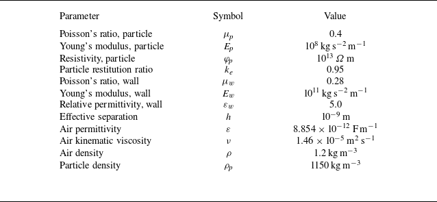
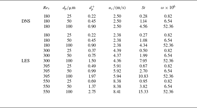
 Reτ=180
 Reτ=180
 Reτ=550

 u¯+
 y+
 Reτ=180
 uτ
 dp=25μm
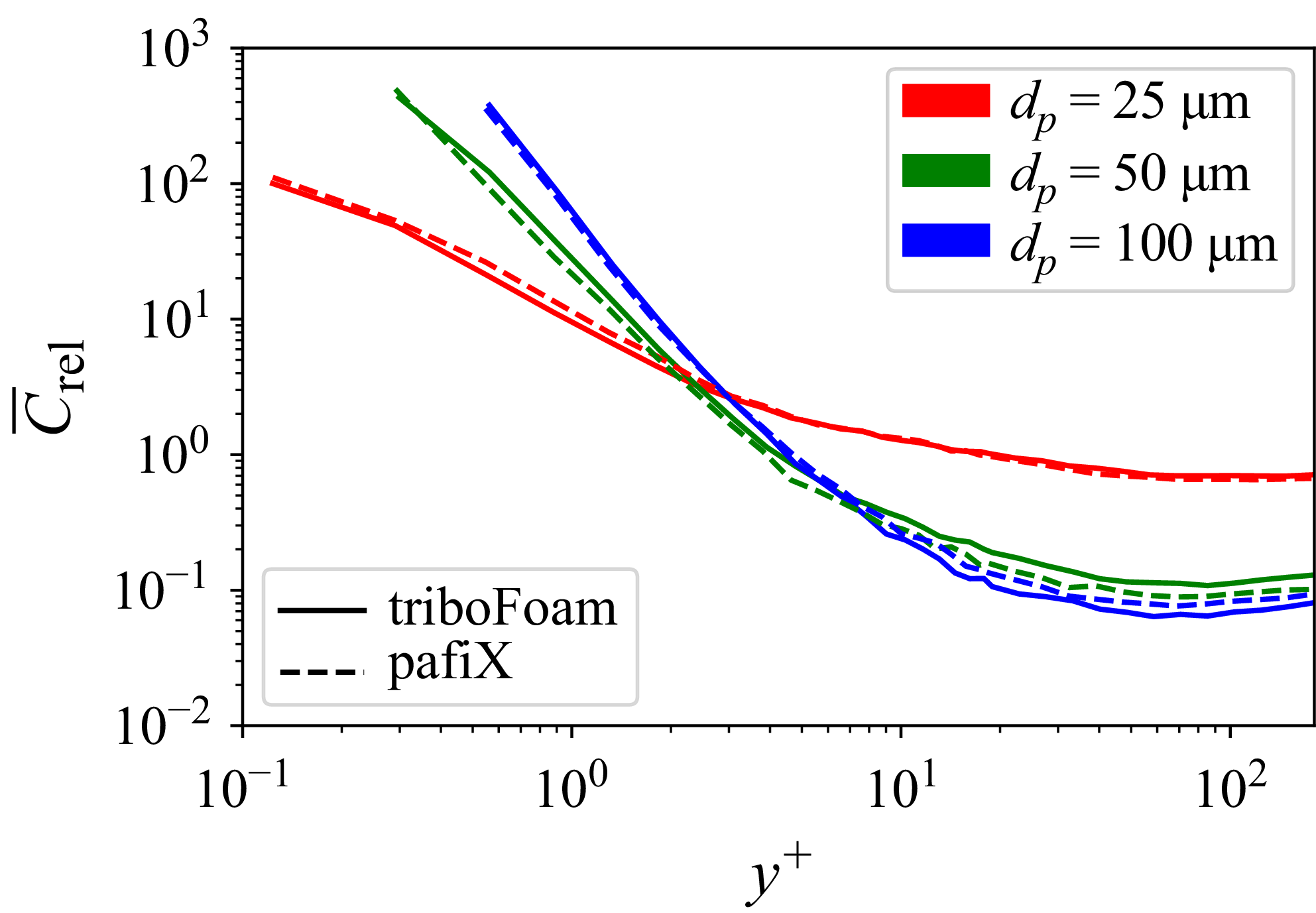
 C¯rel
 y+
 Reτ=180
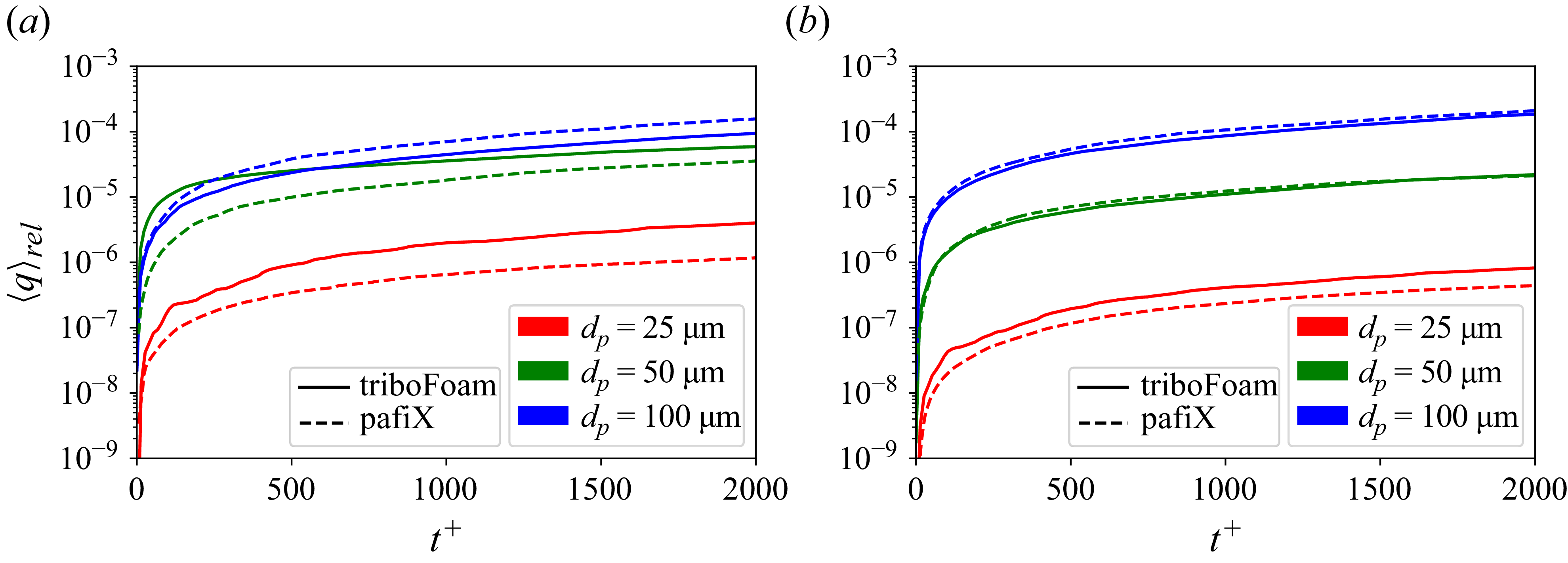
 ⟨q⟩rel
 Reτ=180
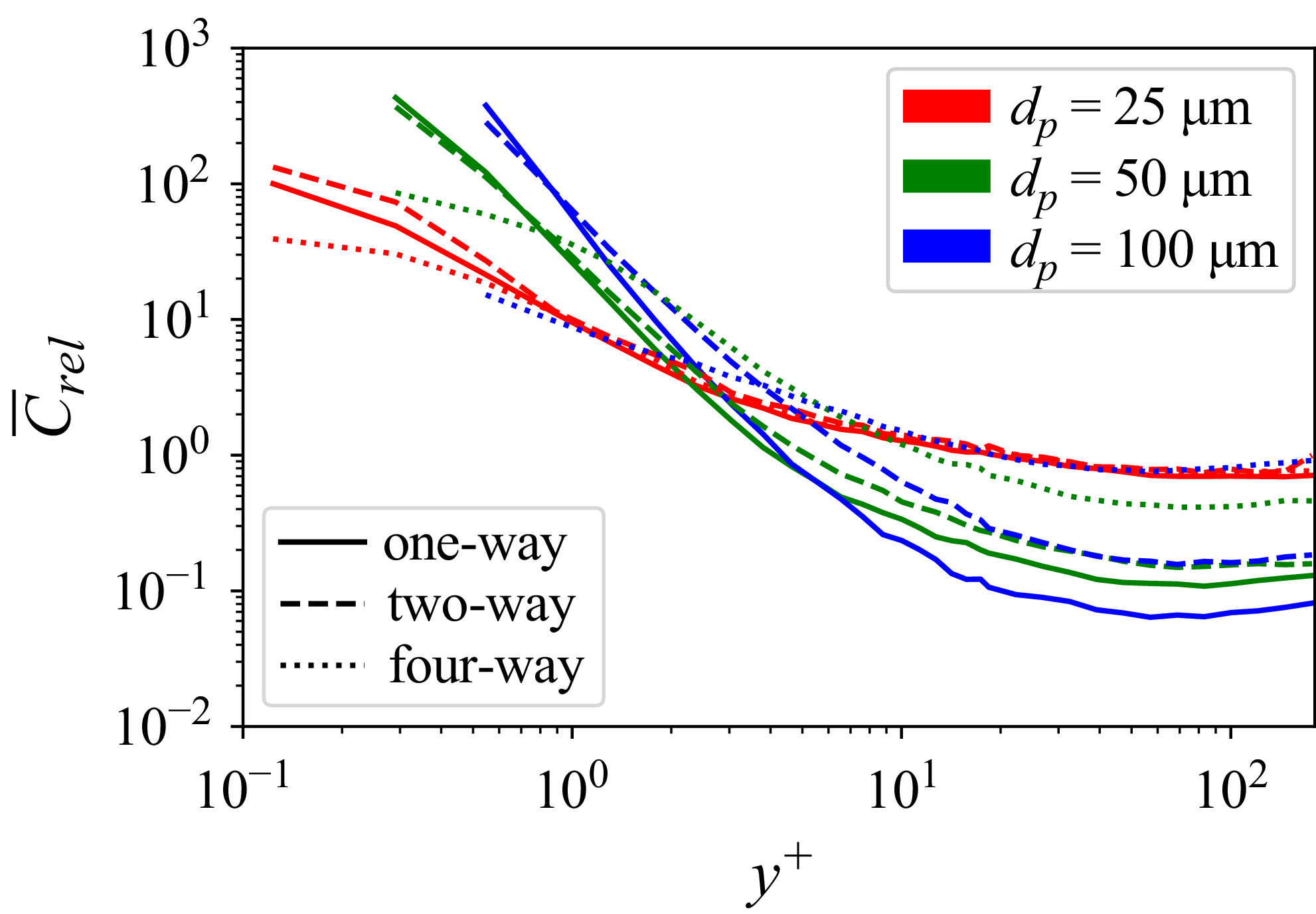
 C¯rel
 y+
 Reτ=180

 ⟨q⟩rel
 ⟨q⟩rel/dt+
 Reτ=180

 ncoll/t+
 ucoll,n+
 Reτ=180

 C¯rel
 y+
 ⟨q⟩rel
 Reτ=180

 ncoll/t+
 ucoll,n+
 Reτ=180

 Crel
 ⟨q⟩rel
 t
 t+

 ncoll/t+
 ucoll,n+
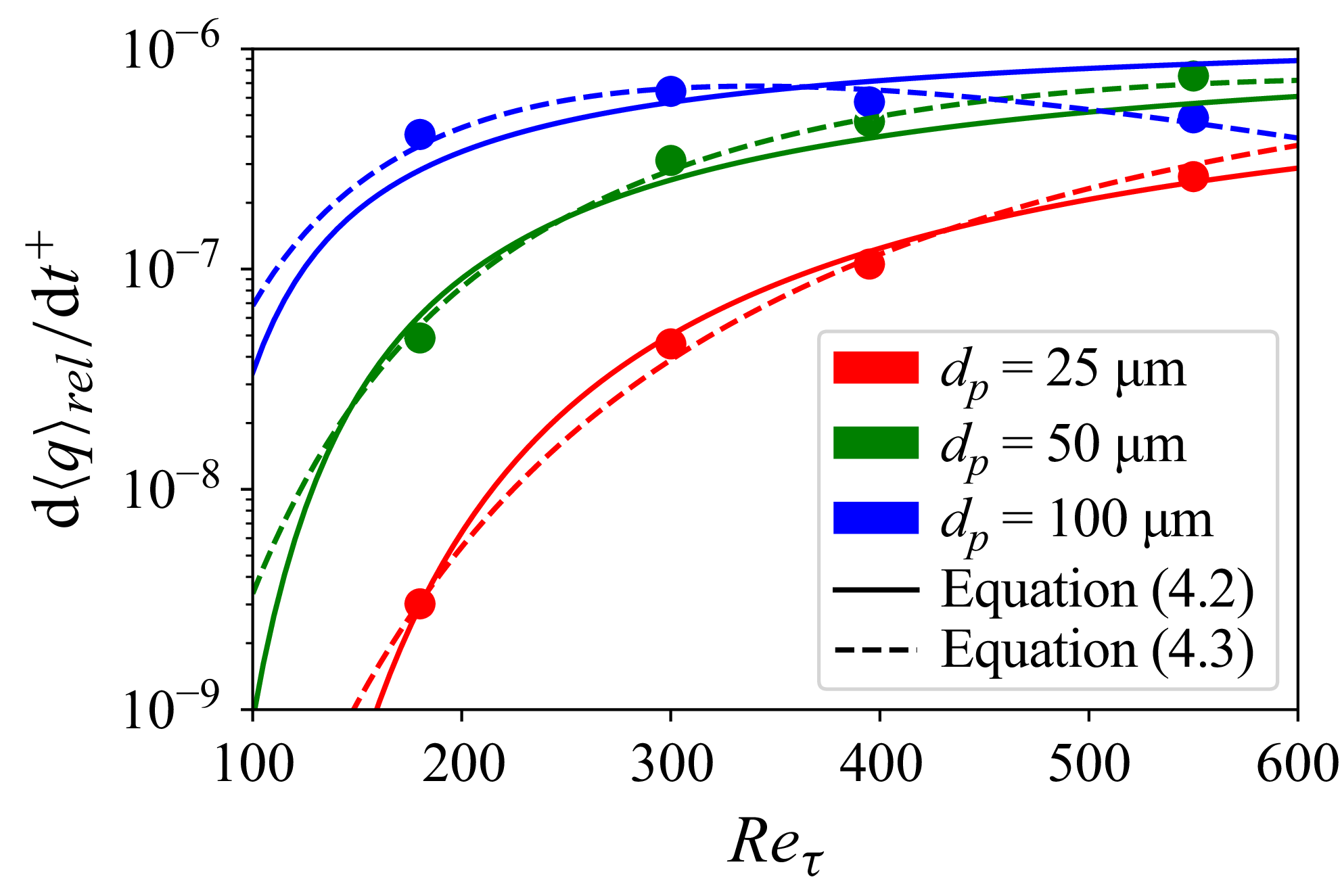
 d⟨q⟩rel/dt

 q¯rel
 Reτ=180

 ucoll,n+
 Reτ=180
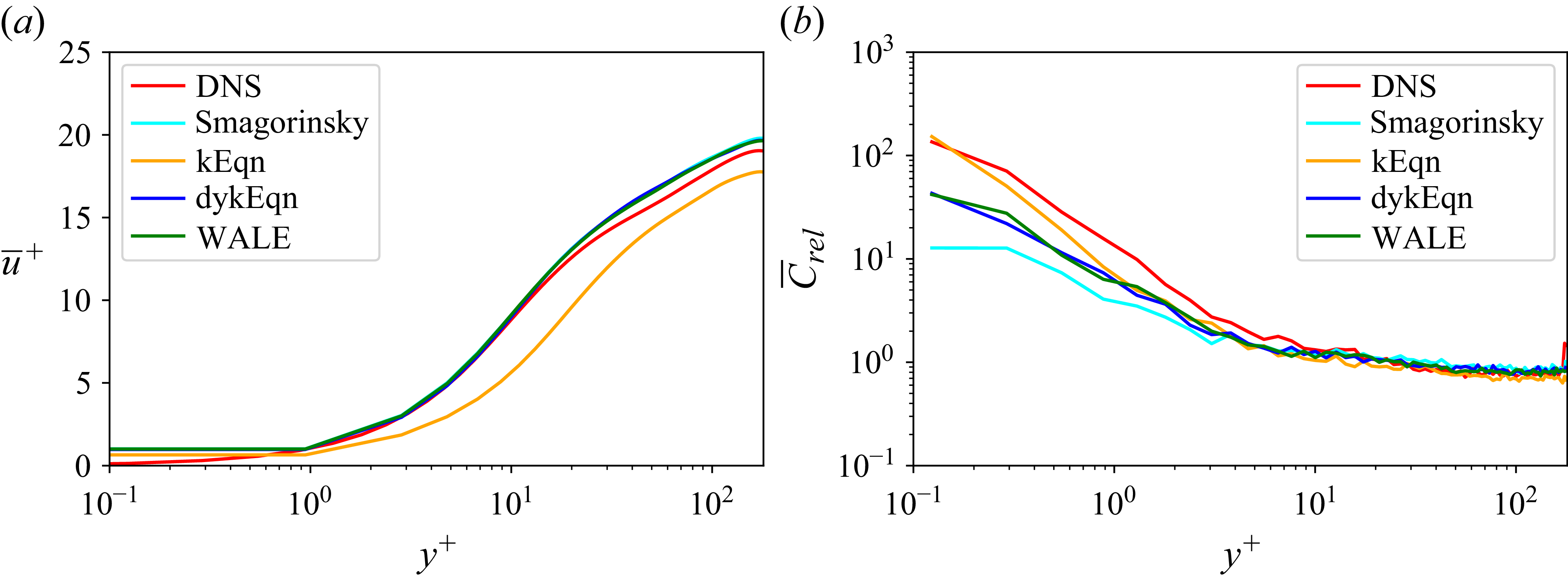
 u¯+
 C¯rel
 y+
 Reτ=180
 dp=25μm
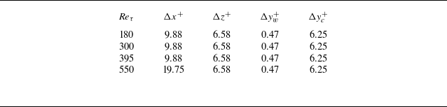
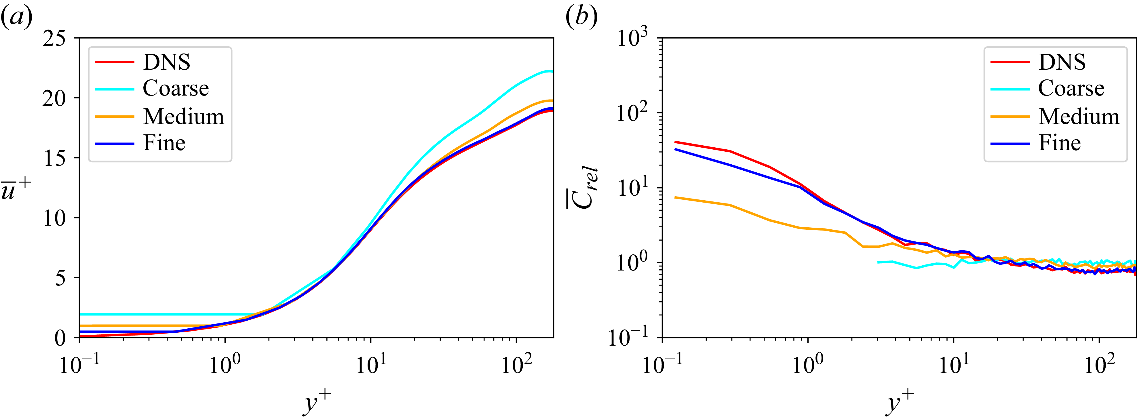
 u¯+
 C¯rel
 y+
 Reτ=180
 dp=25μm

 u¯+
 C¯rel
 y+
 Reτ=300
 dp=25μm
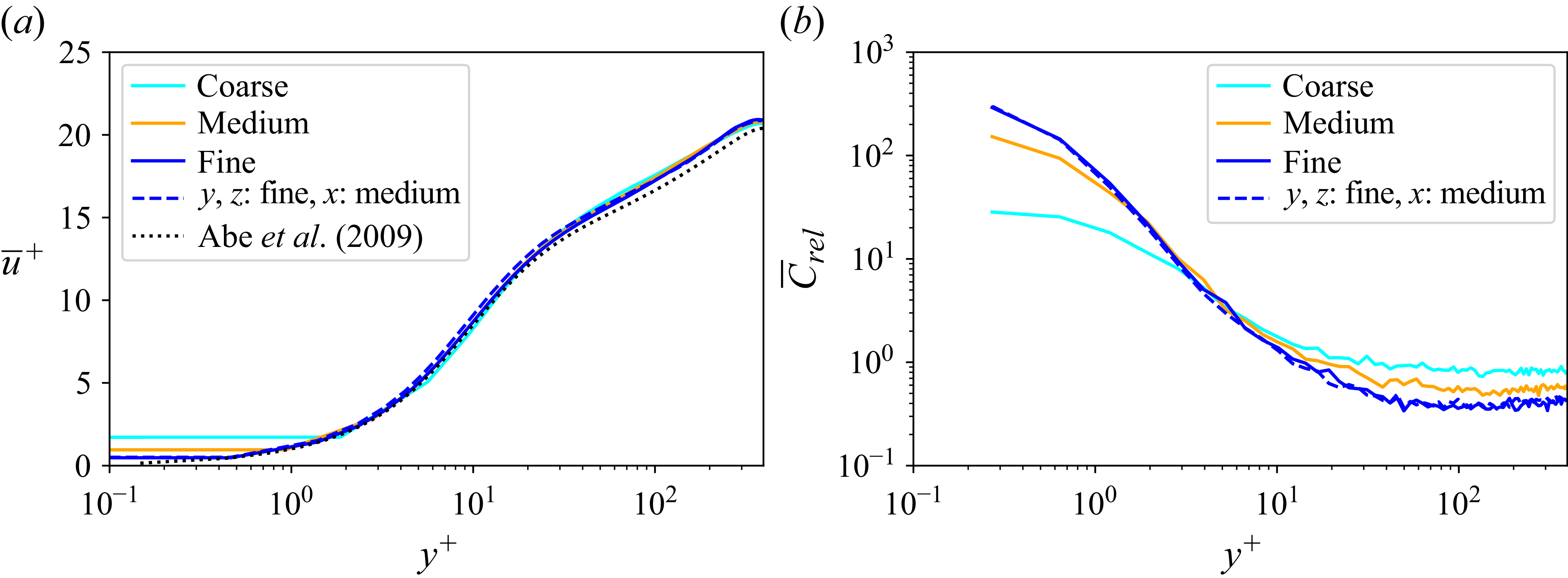
 u¯+
 C¯rel
 y+
 Reτ=395
 dp=25μm
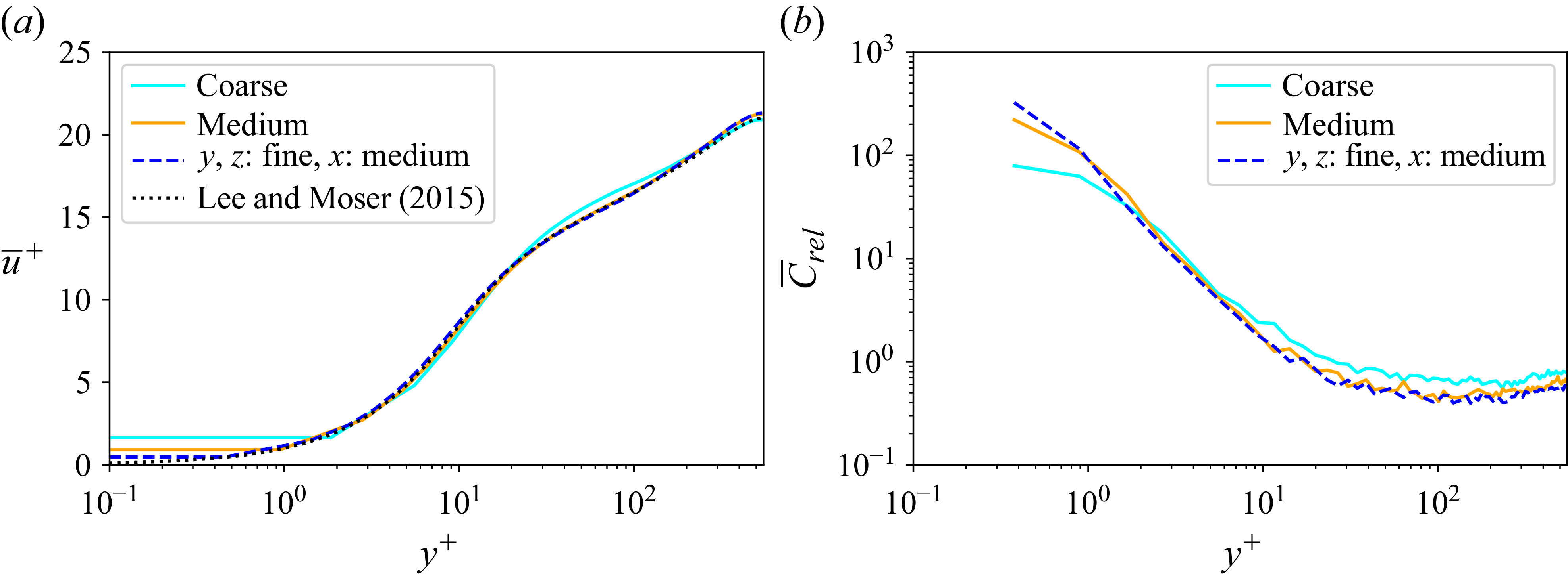
 u¯+
 C¯rel
 y+
 Reτ=550
 dp=25μm
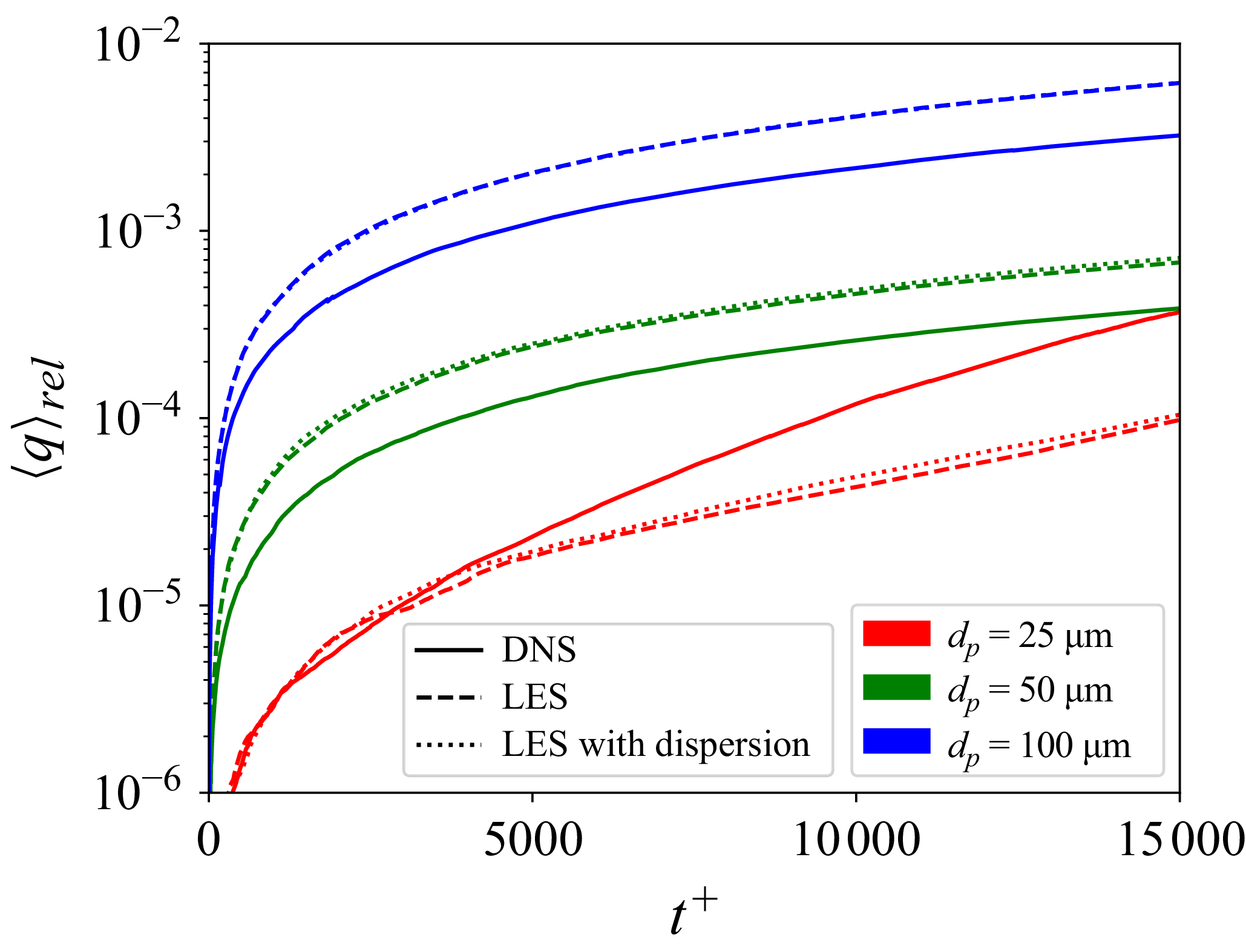
 ⟨q⟩rel
 Reτ=180

 C¯rel
 y+
 ⟨q⟩rel
 Reτ=300
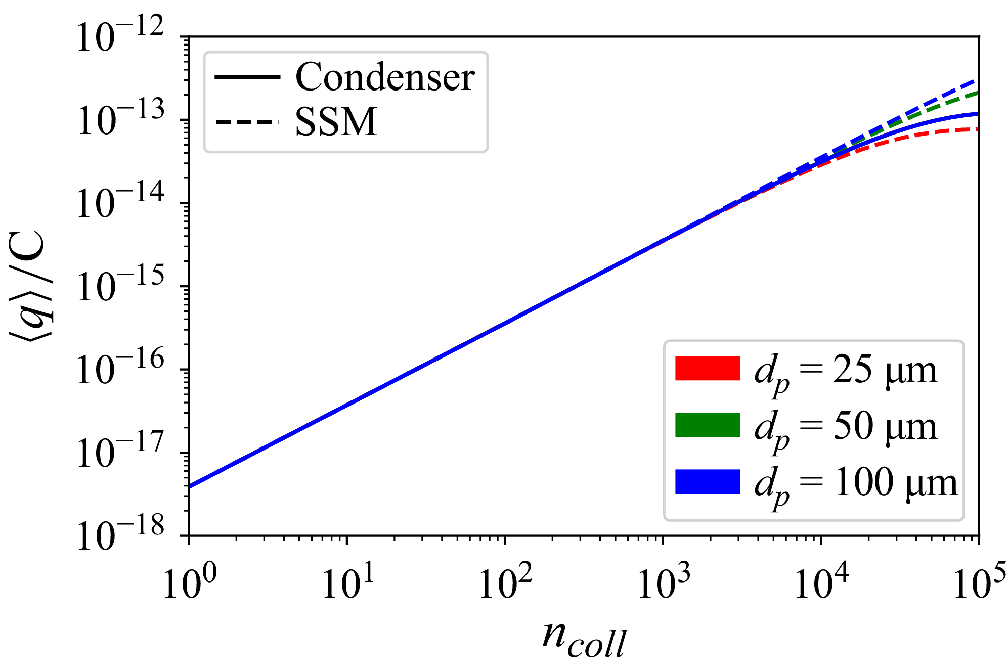
 qsat=1.23×10¹³C
 σ0=γ0=0
 μ0=Δq0,min=μcondenser


