1. Introduction
Nanoscale phase transition plays a vital role in modern thermal management systems, which are essential in applications ranging from high-performance electronics and energy systems to advanced manufacturing (Gong, Hu & Cheng Reference Gong, Hu and Cheng2024). Technologies such as heat pipes, microchannel evaporators, phase-change cooling and thin-film boiling devices rely heavily on accurate modelling of phase transition at liquid–vapour interfaces (Dupont, Thome & Jacobi Reference Dupont, Thome and Jacobi2004; Mukherjee Reference Mukherjee2009; Rana, Lockerby & Sprittles Reference Rana, Lockerby and Sprittles2019; Taassob et al. Reference Taassob, Bordbar, Kheirandish, Zarnaghsh, Kamali and Rana2021). As device sizes shrink and localised heat flux increases, predicting interfacial transport processes with high physical fidelity has become increasingly critical. Accurate modelling of such phenomena requires capturing the interplay between capillarity, surface forces and transport processes within the interfacial region – a challenge that spans from the microscale to the nanoscale (Anderson, McFadden & Wheeler Reference Anderson, McFadden and Wheeler1998; Bhattacharjee et al. Reference Bhattacharjee, Saini, Gupta and Rana2024a ).
A popular theoretical framework for simulating such multiphase systems is provided by the Navier–Stokes–Korteweg (NSK) equations, which originated from the foundational ideas of Gibbs (Reference Gibbs1878) on the concept of a dividing surface, and were later extended through the thermodynamic formulation of diffuse interfaces by van der Waals (Reference Van der and Diederik1979) and Korteweg (Reference Korteweg1901). These pioneering studies established that interfaces possess finite thickness, with van der Waals notably demonstrating how this thickness diverges near critical temperatures using his equation of state. Building upon these classical foundations, modern implementations of the NSK equations augment the classical Navier–Stokes system with a Korteweg stress to represent capillarity in a diffuse interface setting (Anderson et al. Reference Anderson, McFadden and Wheeler1998). In this formulation, the interface is treated as a finite region across which fluid properties vary smoothly, rather than as a sharp boundary (Garcke & Novick-Cohen Reference Garcke and Novick-Cohen2000). Recent advances in numerical methods have significantly enhanced NSK modelling capabilities: Gomez et al. (Reference Gomez, Hughes, Nogueira and Calo2010) employed isogeometric analysis, while Liu et al. (Reference Liu, Gomez, Evans, Hughes and Landis2013) developed a semi-discrete Galerkin method using functional entropy variables. Other notable contributions include Diehl et al. (Reference Diehl, Kremser, Kröner and Rohde2016), who employed a numerical approximation method on the basis of the local discontinuous Galerkin method, Martínez et al. (Reference Martínez, Ramírez, Nogueira, Khelladi and Navarrina2020), who used a high-order finite volume method for phase-change simulations and Tian et al. (Reference Tian, Xu, Kuerten, van der and Jaap2016), who used a adaptive local discontinuous Galerkin method for non-isothermal flows. Contemporary work by Souček et al. (Reference Souček, Heida and Málek2020) on second-law-compliant boundary conditions and Dhaouadi & Dumbser (Reference Dhaouadi and Dumbser2023) on a structure-preserving finite volume scheme further demonstrate the ongoing development of this framework. Despite these advances, the standard NSK formulation assumes density-dependent transport coefficients and omits non-local corrections that become crucial when the interfacial thickness is small – a common situation in nanoscale evaporation and droplet spreading (Anderson et al. Reference Anderson, McFadden and Wheeler1998). Building on the theoretical framework described above, we propose two significant enhancements to the NSK model. First, we introduce a correction term for intermolecular transfer in the momentum equation from higher-order corrections to the momentum balance formulation developed by Struchtrup & Frezzotti (Reference Struchtrup and Frezzotti2022). This modification enables more precise characterisation of momentum exchange at interfaces. Second, we implement density-gradient-dependent transport coefficients – specifically thermal conductivity and viscosity – following the approaches established by Bedeaux, Johannessen & Røsjorde (Reference Bedeaux, Johannessen and Røsjorde2003) and Johannessen & Bedeaux (Reference Johannessen and Bedeaux2004). This implementation better accounts for the influence of microscopic fluid structure on transport phenomena within interfacial regions. Indeed, the sudden density change leads to interfacial resistances that are not captured in the classical Korteweg-type models. Thus, in this study, we develop a modified NSK formulation referred to as the augmented Navier–Stokes–Korteweg (ANSK) model for the remainder of the paper, which specifically addresses the limitations of conventional models when applied to nanoscale interfaces, where interfacial thickness and non-local effects become particularly significant. Further, the effectiveness of the ANSK model is assessed by studying three fundamental problems: Couette flow, pure heat conduction and evaporation from a planar surface. Our results demonstrate the gradient-dependent coefficients effectively increase resistance only in the interface. The coefficients in this phenomenological approach are fitted by comparison with solutions of the Enskog–Vlasov (EV) equation (Struchtrup & Frezzotti Reference Struchtrup and Frezzotti2022) for Couette flow. Application of the fitted equations to heat and mass transfer problems yields excellent agreement to EV simulations – a kinetic theory based approach known for its accuracy but high computational cost (Frezzotti & Sgarra Reference Frezzotti and Sgarra1993; Wu, Zhang & Reese Reference Wu, Zhang and Reese2015). Additionally, we validate the ANSK model by comparing it with molecular dynamics (MD) simulations for the one-dimensional non-evaporative heat conduction case, and observe excellent agreement in both density and temperature profiles. Thus, our ANSK model offers a balanced framework that combines thermodynamic consistency, computational efficiency and improved fidelity for nanoscale transport processes in dense fluids. The structure of the remainder of the paper is as follows: § 2 presents the conservation laws and their corresponding closure relations. In § 3, the ANSK model is introduced. Section 4 is dedicated to the presentation and analysis of three benchmark problems. Finally, concluding remarks are provided in § 5.
2. Conservation laws from the Enskog–Vlasov equation
We begin with the conservation laws for mass, momentum and energy derived from the EV equation (Sobrino Reference Sobrino de1967; Grmela Reference Grmela1971; Struchtrup & Frezzotti Reference Struchtrup and Frezzotti2022). Let
 $\rho$
,
 $\boldsymbol{v}$
,
 $\theta$
,
 $\boldsymbol{\sigma }$
and
 $\boldsymbol{q}$
respectively denote mass density, velocity, temperature (in energy units), trace-free kinetic stress tensor and kinetic heat flux. The conservation equations read
 \begin{align}& \frac {{{\textrm D}}\rho }{{\textrm D}t} + \rho \boldsymbol{\nabla }\boldsymbol{\cdot }\boldsymbol{v} = 0, \quad \rho \frac {{\textrm D}\boldsymbol{v}}{{\textrm D}t} + \boldsymbol{\nabla }(\rho \theta ) + \boldsymbol{\nabla }\boldsymbol{\cdot }\boldsymbol{\sigma } - \rho \boldsymbol{\mathcal{F}} = \boldsymbol{\varUpsilon }^{1}, \end{align}
 \begin{align}&\qquad\quad \frac {3}{2} \rho \frac {{\textrm D}\theta }{{\textrm D}t} + \rho \theta \boldsymbol{\nabla }\boldsymbol{\cdot }\boldsymbol{v} + \boldsymbol{\sigma } : \boldsymbol{\nabla }\boldsymbol{v} + \boldsymbol{\nabla }\boldsymbol{\cdot }\boldsymbol{q} = \varUpsilon ^{2}. \end{align}
The term
 $\boldsymbol{\mathcal{F}}$
, represents the Vlasov force arising from long-range intermolecular interactions (Vlasov Reference Vlasov1961), while the transfer terms
 $\boldsymbol{\varUpsilon }^{1}, \varUpsilon ^{2}$
account for the short-range collisional contributions due to finite-size particle effects and local spatial correlations, as described by the Enskog collision operator (Grmela Reference Grmela1971).
The Vlasov force can be expressed as the divergence of the Korteweg stress tensor
 $(\boldsymbol{\tau }^K)$
as
 $\rho \boldsymbol{\mathcal{F}} = -\boldsymbol{\nabla }\boldsymbol{\cdot }\boldsymbol{\tau }^K$
, where
 $\boldsymbol{\tau }^K$
is given by
 \begin{align} \boldsymbol{\tau }^K = - \frac {2\pi a^3}{3} \frac {\phi _a}{m} \chi _1 \rho ^2 \, \boldsymbol{I} - \frac {2\pi a^5}{15} \frac {\phi _a}{m} \chi _3 \left [ \left ( \rho \boldsymbol{\nabla} ^2 \rho + \frac {1}{2} |\boldsymbol{\nabla }\rho |^2 \right ) \boldsymbol{I} - \boldsymbol{\nabla }\rho \otimes \boldsymbol{\nabla }\rho \right ]. \end{align}
Here,
 $\boldsymbol{I}$
is the identity tensor,
 $\phi _a\gt 0$
characterizes the strength of the attractive part of the Sutherland potential (Sutherland Reference Sutherland1893) and has the same dimensions as temperature,
 $\chi _{1}$
,
 $\chi _{3}$
are the Korteweg coefficients and
 $a$
,
 $m$
are the diameter and mass of the particle respectively.
2.1. Transfer terms from the Enskog collision operator
To close the system in (2.1), constitutive relations and transfer terms must be expressed in terms of known variables. Following the equilibrium formulation of Wang et al. (Reference Wang, Wu, Ho, Li, Li and Zhang2020), the momentum transfer term is modelled as
 \begin{equation} \boldsymbol{\varUpsilon }^{1} = -\frac {2\pi a^3}{3m} \boldsymbol{\nabla }(\rho ^{2} \theta Y) \underbrace {-\frac {4\pi a^3}{15m} \boldsymbol{\nabla }\boldsymbol{\cdot }(\rho Y \boldsymbol{\sigma }) + \boldsymbol{\nabla }\boldsymbol{\cdot }\boldsymbol{\varPhi }^{(4)}}, \end{equation}
where the last two terms above the underbrace have been modelled following Struchtrup & Frezzotti (Reference Struchtrup and Frezzotti2022), who take into account the non-equilibrium effects. Here
 \begin{align} \boldsymbol{\varPhi }^{(4)} = \frac {4 \sqrt {\pi } a^{4}}{15 m} \biggl [ \boldsymbol{I}{\kern-1pt}\rho ^{2} Y \sqrt {\theta } (\boldsymbol{\nabla }\boldsymbol{\cdot }\boldsymbol{v}) + \rho ^{2} Y \sqrt {\theta } \boldsymbol{\nabla }\boldsymbol{v} + \rho ^{2} Y \sqrt {\theta } (\boldsymbol{\nabla }\boldsymbol{v})^{\mathsf{T}} \biggr ], \end{align}
whose divergence is the second-order symmetric derivative of velocity – fourth-order correction term in
 $a$
, following Struchtrup & Frezzotti (Reference Struchtrup and Frezzotti2022). The effect of this term considered in the ANSK model shall be discussed in detail in sections to follow.
In a similar manner the energy transfer term following the equilibrium formulation of Wang et al. (Reference Wang, Wu, Ho, Li, Li and Zhang2020) is modelled as
 \begin{align} \varUpsilon ^{2} = -\frac {2 \pi }{3 }\frac {a^{3}}{m}\rho ^{2} \theta Y(\boldsymbol{\nabla }\boldsymbol{\cdot }\boldsymbol{v}). \end{align}
Here,
 $ Y(\rho )$
is the pair correlation function at contact, given by Carnahan & Starling (Reference Carnahan and Starling1969) as
 \begin{align} Y = \frac {1}{2} \frac {2 - \eta }{(1 - \eta )^3}, \quad {\text{where}\,\eta = \frac {\pi a^3 \rho }{6 m}\,\text{is the fluid reduced density}.} \end{align}
Second law of thermodynamics: Assuming entropy depends only on
 $ \rho$
and
 $ \theta$
, we postulate the following functional form for the entropy:
 \begin{equation} \varsigma (\rho , \theta ) = \frac {3}{2} \ln \theta - \ln \rho - g(\rho ), \quad g(\rho ) = \frac {2}{3} \frac {\pi a^3}{m} \int Y(\rho ) \, {\textrm d}\rho . \end{equation}
Using the Gibbs relation and substituting from the conservation laws, the entropy balance gives
 \begin{equation} \rho \frac {{\textrm D}\varsigma }{{\textrm D}t} + \boldsymbol{\nabla }\boldsymbol{\cdot }\left ( \frac {\boldsymbol{q}}{\theta } \right ) = - \frac {1}{\theta } \boldsymbol{\sigma } : \boldsymbol{\nabla }\boldsymbol{v} - \frac {1}{\theta ^2} \boldsymbol{q} \boldsymbol{\cdot }\boldsymbol{\nabla }\theta = \varSigma . \end{equation}
Entropy production is non-negative when the following constitutive relations hold:
 \begin{align} \boldsymbol{\sigma } = -\mu \left ( \boldsymbol{\nabla }\boldsymbol{v} + (\boldsymbol{\nabla }\boldsymbol{v})^{\mathsf{T}} \right ) + \frac {2}{3} \mu \left ( \boldsymbol{\nabla }\boldsymbol{\cdot }\boldsymbol{v} \right ) \boldsymbol{I}, \quad \boldsymbol{q} = -\lambda \boldsymbol{\nabla }\theta , \end{align}
where
 $ \mu \gt 0$
,
 $ \lambda \gt 0$
are the shear viscosity and thermal conductivity, respectively. Thus, entropy production
 $ \varSigma \geqslant 0$
is guaranteed, proving the second law of thermodynamics, and the entropy flux is identified as
 $ \boldsymbol{\varPsi } = \boldsymbol{q}/\theta$
. Together, the conservation laws (2.1), and constitutive relations (2.9) form a closed NSK-type system derived from the EV framework.
3. Augmented Navier–Stokes–Korteweg model
The conservation laws for mass, momentum and energy in conservative form are given by
 \begin{align} \frac {\partial \rho }{\partial t} + \boldsymbol{\nabla }\boldsymbol{\cdot }(\rho \boldsymbol{v}) = 0, \quad \rho \frac {{\textrm D} \boldsymbol{v}}{{\textrm D}t} + \boldsymbol{\nabla }\boldsymbol{\cdot }\boldsymbol{\varPi } = \boldsymbol{0},\quad \rho \frac {{\textrm D}}{{\textrm D}t} \left ( \dfrac {3}{2} \theta + \dfrac {1}{2} |\boldsymbol{v}|^2 + \varepsilon _K \right ) + \boldsymbol{\nabla }\boldsymbol{\cdot }\boldsymbol{\mathcal{J}} = 0, \end{align}
where the total momentum and energy flux are defined as
 \begin{align} \boldsymbol{\varPi } &= \left [ \rho \theta + \frac {2\pi a^3}{3m} \rho ^2 \theta Y \right ] \boldsymbol{I} + \left (1 + \frac {4\pi a^3}{15m} \rho Y \right ) \boldsymbol{\sigma } + \boldsymbol{\tau }^K - \boldsymbol{\varPhi }^{(4)}, \end{align}
 \begin{align} \boldsymbol{\mathcal{J}} &= \boldsymbol{q} + \boldsymbol{q}^K + \bigl(\rho \theta \boldsymbol{I} + \boldsymbol{\sigma } + \boldsymbol{\tau }^K\bigr) \boldsymbol{\cdot }\boldsymbol{v} + {\underbrace {\frac {2\pi }{3}\frac {a^{3}}{m} \rho Y \left ( \rho \theta \boldsymbol{v} + \frac {2}{5} \boldsymbol{\sigma } \boldsymbol{\cdot }\boldsymbol{v} \right ),}} \end{align}
where the terms within the brace in (3.3) have been obtained following the formulation as modelled in Struchtrup & Frezzotti (Reference Struchtrup and Frezzotti2022). The potential energy due to the attractive forces (Anderson et al. Reference Anderson, McFadden and Wheeler1998) and the additional energy flux due to non-local effects (Giovangigli Reference Giovangigli2020) are
 \begin{equation} \varepsilon _K = -\frac {2\pi a^3}{3m} \chi _1 \phi _a \rho + \frac {\pi a^5}{15m} \chi _3 \phi _a \frac {1}{\rho } |\boldsymbol{\nabla }\rho |^2, \quad \boldsymbol{q}^K = \frac {2\pi a^5}{15m} \chi _3 \phi _a \rho (\boldsymbol{\nabla }\rho )(\boldsymbol{\nabla }\boldsymbol{\cdot }\boldsymbol{v}). \end{equation}
To incorporate interfacial and non-equilibrium effects, the transport coefficients – thermal conductivity
 $ \lambda$
and viscosity
 $ \mu$
– are modified to depend on both the local density and its gradient. Such dependencies become significant near phase interfaces, as discussed in Bedeaux et al. (Reference Bedeaux, Johannessen and Røsjorde2003) and Johannessen & Bedeaux (Reference Johannessen and Bedeaux2004). The expressions for
 $ \lambda$
and
 $ \mu$
are given by
 \begin{align} \lambda \left (\rho , |\boldsymbol{\nabla }\rho |\right ) &= \frac {15}{4} \frac {\rho \theta \left (1+{\dfrac {2\pi }{5}\dfrac {a^{3}}{m}\rho Y}\right )^{2}}{\dfrac {16}{5}\dfrac {\rho }{m}\sqrt {\pi \theta }a^{2}{Y}\underbrace {\left [1+ \alpha \left (\frac {a}{\rho }|\boldsymbol{\nabla }\rho |\right )^{2}\right ]^{2}}} + {\frac {2}{3} \frac {a^{4}\sqrt {\pi \theta }}{m}\rho ^{2} Y}, \end{align}
 \begin{align} \mu \left (\rho , |\boldsymbol{\nabla }\rho |\right ) &= \frac {\rho \theta \left (1+{\dfrac {4\pi }{15}\dfrac {a^{3}}{m}\rho Y}\right )^{2}}{\dfrac {16}{5}\dfrac {\rho }{m}\sqrt {\pi \theta }a^{2}{Y}\underbrace {\left [1+ \alpha \left (\frac {a}{\rho }|\boldsymbol{\nabla }\rho |\right )^{2}\right ]^{2}}} + {\frac {4}{15} \frac {a^{4}\sqrt {\pi \theta }}{m}\rho ^{2} Y}, \end{align}
where the coefficient
 $ \alpha$
is a temperature-dependent parameter, detailed in later sections. Interfacial modifications arising from density gradients are highlighted via the underbrace, marking non-equilibrium contributions in the interfacial region.
The ANSK model thus consists of the conservation laws (3.1), constitutive relations (2.9) and modified transport coefficients (3.5)–(3.6), all formulated to satisfy the second law of thermodynamics by ensuring non-negative entropy production. A system that meets this criterion is referred to as thermodynamically consistent.
The requirements on the modified transport coefficients (3.5)–(3.6) are (i) recovery of the correct bulk liquid and vapour transport coefficients, and (ii) reduced transport across the interfacial region, thereby reproducing the principal behaviour of the original EV equation. The adopted functional form satisfies both criteria. While alternative forms could be considered, all admissible choices lead to similar transport-coefficient profiles, characterised by systematically lower values within the interfacial zone.
Phase transition in equilibrium: in equilibrium, the momentum balance equation, the second equation in (3.1), yields the thermal equation of state
 \begin{align} p(\rho ,\theta ) = \rho \theta \left (1 + \frac {2\pi }{3} \rho Y \right ) - \frac {2\pi }{3} \chi _1 \rho ^2, \end{align}
which describes pressure as a non-monotonic function. This behaviour is analogous to the van der Waals equation of state and permits phase separation, as discussed in Struchtrup (Reference Struchtrup2024). Introducing the specific volume
 $ v = {1}/{\rho }$
, the critical point is determined from the conditions
 \begin{align} \left . \frac {\partial p}{\partial v} \right |_{\theta , {\textit{crit}}} = 0 \quad \text{and} \quad \left . \frac {\partial ^2 p}{\partial v^2} \right |_{\theta , {\textit{crit}}} = 0, \end{align}
which yield the critical temperature, pressure and volume as
 $ \theta _{\textit{critical}} = 0.7546$
,
 $ p_{\textit{critical}} = 0.06748$
and
 $ v_{\textit{critical}} = 4.014$
, respectively.
Maxwell’s equal area rule (Struchtrup Reference Struchtrup2024) is applied to determine the conditions for phase coexistence below the critical temperature. The rule is expressed as
 \begin{align} \int _{v_l}^{v_v} p(\theta , v) \, {\textrm d}v = p_{\textit{sat}} (v_v - v_l), \end{align}
and is evaluated over a range of subcritical temperatures to generate a collection of data points for the saturation pressure
 $p_{\textit{sat}}(\theta )$
, along with the corresponding specific volumes of the liquid and vapour phases, given by
 $v_l(\theta ) = 1/\rho _l(\theta )$
and
 $v_v(\theta ) = 1/\rho _v(\theta )$
, respectively. Here,
 $\rho _l(\theta ) \equiv \rho _l^{\textit{sat}}(\theta )$
and
 $\rho _v(\theta ) \equiv \rho _v^{\textit{sat}}(\theta )$
represent the saturated densities of the liquid and vapour phases, respectively.
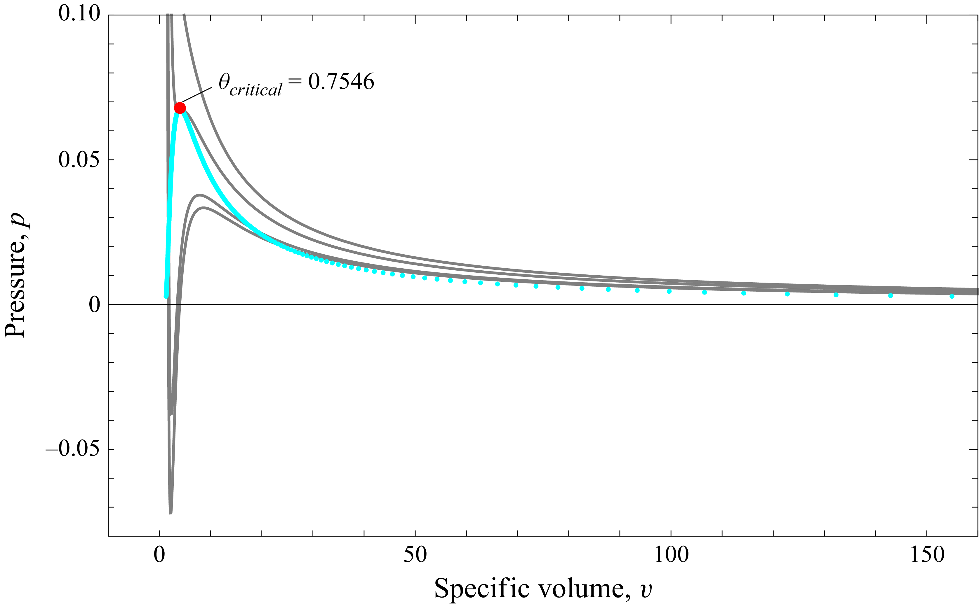
These results are illustrated in figure 1, which displays a
 $p$
–
 $v$
diagram. The saturation curve for the liquid and vapour phases is plotted in cyan, and the isothermal pressure curves
 $p(\theta , v)$
, obtained from (3.7), are shown in grey. The isotherms for temperatures below the critical point clearly exhibit the familiar non-monotonic behaviour that signals the presence of a phase transition.
The saturation curve is shown in cyan, with grey lines depicting isotherms at
 $ \theta = 0.85, 0.75,{} 0.63, 0.60$
, arranged from top to bottom in the
 $ p$
–
 $ v$
diagram. The critical point is indicated by a red marker.

4. Application of NSK model to three benchmark problems
4.1. Two-phase isothermal Couette flow
To validate the ANSK model, we simulate steady, isothermal Couette flow across a liquid–vapour interface and compare results with direct simulation Monte Carlo (DSMC) benchmarks (Rah & Eu 2001; Frezzotti et al. Reference Frezzotti and Rossi2012). For the physical set-up, we define a coordinate system where the interface normal is aligned with the
 $ x$
-axis. The liquid phase is located in the region
 $ \varOmega = \{(x, y, z) \in \mathbb{R}^3 : 0 \leqslant x \lt x_l\}$
, where
 $x_l$
represents both the upper spatial limit of the liquid region and its nominal thickness. The vapour phase occupies the region to the right of this interface. Flow is unidirectional parallel to the liquid–vapour interface with
 $ \boldsymbol{v}(x) = (0, v_y(x), 0)$
, where
 $ v_y(0) = 0$
and
 $ \textrm{d}{\kern0.5pt}v_y/\textrm{d}{\kern0.5pt}x \to {const}$
as
 $ x \to L$
. The incompressible and steady flow satisfies
 $ \boldsymbol{\nabla }\boldsymbol{\cdot }\boldsymbol{v} = 0$
, so the governing variables reduce to {
 $ \rho (x), v_y(x), \sigma _{xy}(x)$
}.
All variables are non-dimensionalised by setting
 $ a = m = \phi _a = 1$
. Accordingly, length
 $ x$
is scaled by the particle diameter
 $ a$
, density
 $ \rho$
by
 $ m/a^3$
, velocity
 $v$
by the square root of the potential strength
 $ \phi _a$
, i.e.
 $\sqrt { \phi _a}$
, and temperature
 $ \theta$
by the potential strength
 $ \phi _a$
. All equations and results that follow are presented in this dimensionless form. The ANSK model reduces to
 \begin{align} \frac {{\textrm d}}{{\textrm d}x}\left \{ \left [1 + \frac {4\pi }{15} \rho Y \right ] {\sigma _{xy}} - \frac {4 \sqrt {\pi }}{15} \rho ^2 Y \sqrt {\theta } \frac {{\textrm d} v_{y}}{{\textrm d}x} \right \} &= 0, \quad \mu \frac {{\textrm d} v_{y}}{{\textrm d}x} + {\sigma _{{xy}}} = 0. \end{align}
The Korteweg coefficients are specified as
 $\chi _{1} =2$
and
 $\chi _{3}$
as a temperature-dependent function defined as
 ${\chi }_{3}(\theta ) = c_{0}+c_{1}\theta +c_{2}\theta ^{2}+c_{3}\theta ^{3}$
, expressed as a function of
 $\theta$
(for details refer to Bhattacharjee et al. Reference Bhattacharjee, Struchtrup and Singh Rana2024b
). Here,
 $c_{0} = -2.25557$
,
 $c_{1} = 18.2905$
,
 $c_{2} = -25.0087$
and
 $c_{3} = 18.1759$
. Equations (4.1) are discretised using midpoint schemes (Ascher & Petzold Reference Ascher and Petzold1998), with a uniform mesh in
 $ x \in [0, L]$
, with
 $L=50$
.
In our simulations, we use
 $ n = 1250$
grid points across the domain, which corresponds to 25 grid points per molecular diameter, since the molecular diameter
 $ a$
is set to unity in the non-dimensionalisation.
Boundary conditions:
 $ v_y(0) = 0, \quad \left .\sigma _{xy} \right |_{x=L}= \text{assigned constant}, \quad \left . {{\textrm d}\sigma _{xy}}/{{\textrm d}x} \right |_{x=0,L} = 0.$
Density- and gradient-dependent coefficients use equilibrium values from (3.1), evaluated as in Frezzotti, Gibelli & Lorenzani (Reference Frezzotti, Gibelli and Lorenzani2005), Struchtrup & Frezzotti (Reference Struchtrup and Frezzotti2022) and Bhattacharjee et al. (Reference Bhattacharjee, Struchtrup and Singh Rana2024b
). The resulting system of linear equations is solved numerically using
 $\textrm {MATLAB}^{\circledR }$
. The parameter
 $\alpha$
is varied with the dimensionless temperature
 $\theta$
by fitting it to match the EV equation solutions for the Couette flow problem, following Struchtrup & Frezzotti (Reference Struchtrup and Frezzotti2022).
4.1.1. Analysis of results of the two-phase Couette flow
Figure 2 presents the velocity profiles
 $v_y(x)$
for dimensionless temperatures
 $\theta = 0.55$
,
 $0.60$
and
 $0.65$
, along with the shear stress
 $\sigma _{xy}(x)$
at
 $\theta = 0.65$
, compared against EV-DSMC data (black diamonds). The ANSK model (black solid line) shows excellent agreement with DSMC results, reflecting improved interface resistance from the temperature-dependent fitting of
 $\alpha$
in the modified NSK framework. In contrast, model 1 (
 $\alpha = 0$
), which corresponds to the conventional NSK formulation, fails to resolve the sharp interfacial gradients observed at temperatures far from the critical point (red dashed line). Its performance improves as
 $\theta$
approaches the critical point, where the interface becomes inherently smoother and thicker.
Although the fitted value of
 $ \alpha = 1.925$
at
 $ \theta = 0.65$
is markedly above zero, its effect on the transport coefficients is minimal due to the small density gradients near the critical point. The underbraced gradient-dependent correction term in (3.5) and (3.6) becomes negligible when
 $ |\boldsymbol{\nabla }\rho |$
is small, even if
 $ \alpha$
is large. This explains why both the ANSK model and model 1 produce similar shear velocity profiles at
 $ \theta = 0.65$
, despite having different values of
 $ \alpha$
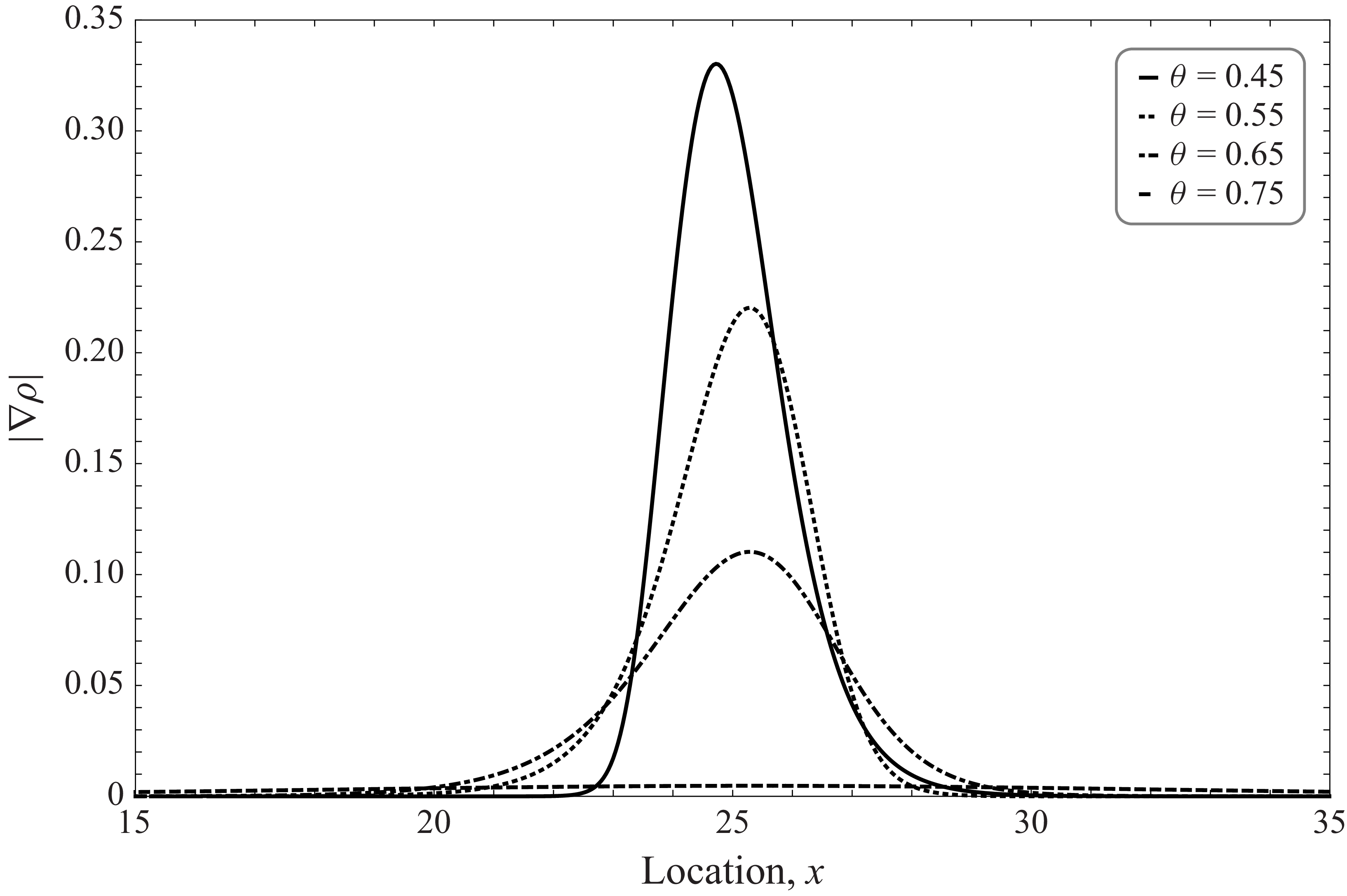
. This observation is further supported by the density gradient profiles plotted at various temperatures (
 $ \theta = 0.45, 0.55, 0.65, 0.75$
), shown in figure 3, which demonstrate a clear decrease in
 $ |\boldsymbol{\nabla }\rho |$
as
 $ \theta$
approaches the critical value.
Two-phase Couette flow: comparison of EV-DSMC (black diamonds), ANSK model (black solid line), model 1 (red dashed line) and model 2 (blue dot-dashed line). (a) Velocity profiles for
 $\theta = 0.55$
(b) Velocity profiles for
 $\theta = 0.60$
(c) Velocity profiles for
 $\theta =0.65$
(top row and bottom left); shear stress at
 $\theta = 0.60$
(bottom right).

Profiles of the density gradient
 $ |\boldsymbol{\nabla }\rho (x)|$
across the liquid–vapour interface for different dimensionless temperatures
 $ \theta = 0.45, 0.55, 0.65, 0.75$
.

Model 2, which omits the fourth-order correction term in
 $a$
,
 $\boldsymbol{\varPhi }^{(4)}$
, results in notable discrepancies in both velocity and stress fields (blue dot-dashed line), underscoring the importance of this term.
The shear stress is largely independent of
 $\alpha$
, depending instead on the higher-order correction. However, the inclusion of
 $\alpha$
in the transport coefficients is essential for capturing sharp interface transitions at subcritical temperatures. To determine a suitable temperature-dependent form of
 $\alpha$
, Couette flow simulations are conducted over a range of
 $\theta$
. A fitting procedure is then employed to match these results with solutions of the EV equation, following the approach outlined by Struchtrup & Frezzotti (Reference Struchtrup and Frezzotti2022). This yields the following empirical relation for
 $\alpha$
as a function of temperature
 \begin{equation} \alpha (\theta ) = 9.5\theta - 4.25, \quad 0.45 \lt \theta \lt 0.7546. \end{equation}
This fitted relation is then used in all subsequent analysis.
4.2. Transport-coefficient properties
To examine whether the viscosity in the bulk region captures the characteristic temperature-dependent behaviour observed in real fluids, we analyse the variation of viscosity in both the saturated liquid and vapour phases over a range of subcritical temperatures. In real fluids, liquid viscosity
 $(\mu _{l})$
, generally decreases with increasing temperature, whereas the viscosity of dilute gases
 $(\mu _{v})$
, shows the opposite trend. In our model, the coefficient of viscosity
 $\mu (\rho , |\boldsymbol{\nabla }\rho |)$
depends on both local density and its gradient, as defined in (3.6). To evaluate whether this formulation recovers the expected trends in bulk phases, we utilise saturation data obtained through Maxwell’s equal area construction. As shown in the
 $p$
–
 $v$
diagram of figure 1, isotherms in the liquid region are nearly vertical near the saturation curve, suggesting that density remains approximately constant along an isotherm. Therefore, the liquid viscosity may be approximated by evaluating
 $\mu$
at the saturated liquid density, i.e.
 $\mu _{l}(\theta ) \approx \mu (\rho _l^{\textit{sat}}(\theta ), \theta )$
. In contrast, the vapour isotherms are nearly horizontal, indicating nearly constant pressure and allowing a similar approximation for the vapour phase,
 $\mu _{v}(\theta ) \approx \mu (\rho _v^{\textit{sat}}(\theta ), \theta )$
.
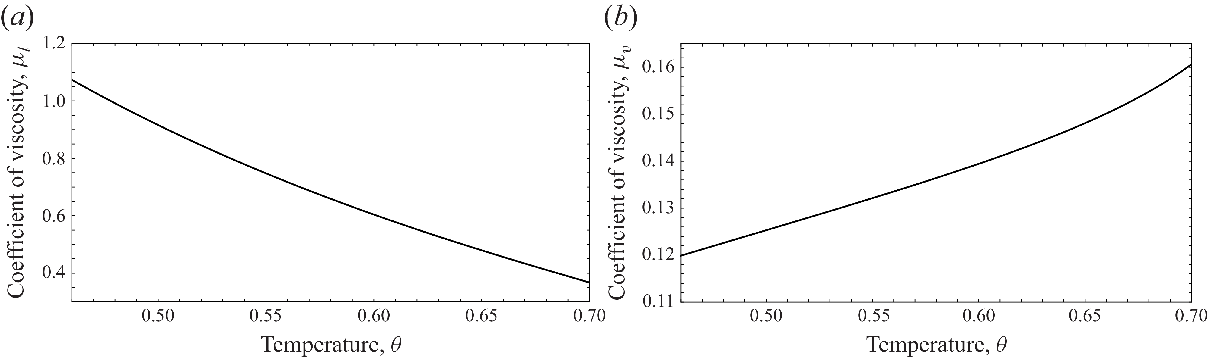
Profiles of the coefficient of viscosity for liquid
 $\mu _{l}$
, and vapour
 $\mu _{v}$
versus dimensionless temperature
 $\theta$
.

Following this approach, we compute the viscosities of the liquid and vapour phases at various temperatures using the corresponding saturated densities. The resulting trends, presented in figure 4, clearly show that the liquid viscosity decreases with increasing temperature, while the vapour viscosity increases – thus reproducing the classical behaviour. To further clarify the temperature dependence of the viscosity, we note that, along the saturation line, both temperature and density vary, and hence viscosity cannot be regarded as a function of temperature alone. To isolate the true temperature dependence, we evaluate the viscosity at constant pressure for both liquid and vapour phases. In the bulk region, the viscosity obtained from (3.6) may thus be expressed as a function of pressure and density as
 \begin{align} \mu (p,\rho ) &= \sqrt {\dfrac {p+\dfrac {2 \pi }{3}\chi _{1}\rho ^{2}}{\rho \left (1+\dfrac {2\pi }{3}\rho Y\right )}}\left \{\dfrac {\left (1+\dfrac {4\pi }{15}\dfrac {a^{3}}{m}\rho Y\right )^{2}}{\dfrac {16}{5}\dfrac {1}{m}\sqrt {\pi }a^{2}Y} + \dfrac {4}{15} \dfrac {a^{4}\sqrt {\pi }}{m}\rho ^{2} Y\right \}\!, \end{align}
and the corresponding temperature follows from the equation of state (3.7) as
 \begin{align} \theta (p,\rho ) &= \frac {p+\dfrac {2 \pi }{3}\chi _{1}\rho ^{2}}{\rho \left (1+\dfrac {2\pi }{3}\rho Y\right )}. \end{align}
Figure 5 presents the variation of the viscosity coefficient as a function of temperature for fixed pressures from sub- to supercritical. The curves result from (4.3) and (4.4) by using density as a curve parameter. The plot demonstrates that, at fixed pressure
 $p_{0}$
(say), the viscosity in the liquid phase decreases with increasing temperature, whereas the viscosity in the vapour phase increases with temperature. These results confirm that the viscosity reproduces the correct thermophysical trends when temperature is varied independently of density or pressure effects, consistent with established experimental observations for real fluids.
Coefficient of viscosity as a function of temperature at constant pressure. The bottom red solid curve is the ideal gas case where viscosity is independent of pressure.

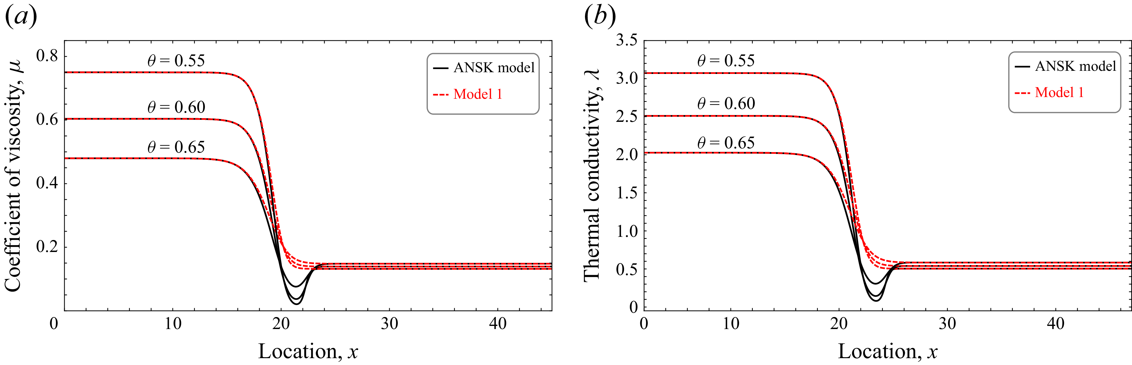
Comparison of coefficient of viscosity (a) and thermal conductivity (b) computed from ANSK model (black solid line) and model 1 (red dashed line) for
 $\theta = 0.55, 0.60\, \text{and}\,0.65$
.

In the present formulation, the non-local correction appears in the denominator of the transport coefficients. This may seem different from the additive corrections introduced in Bedeaux et al. (Reference Bedeaux, Johannessen and Røsjorde2003) and Johannessen & Bedeaux (Reference Johannessen and Bedeaux2004). However, it should be noted that their correction applies to the bulk resistances, which are the inverses of the transport coefficients we use in this study. Therefore, the form used here is not fundamentally different but represents the same kind of modification.
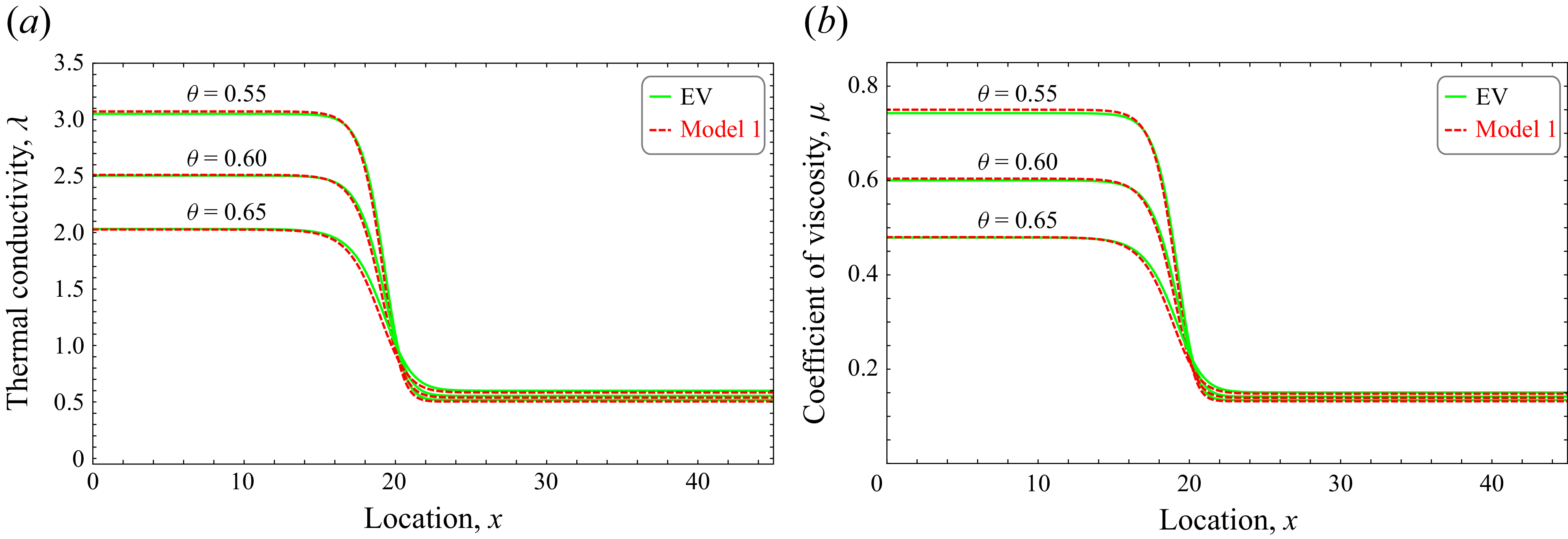
To illustrate the impact of this correction, figure 6 shows a comparison between the viscosity profiles and thermal-conductivity profiles predicted by the ANSK model and model 1 at
 $\theta = 0.55, 0.60\,\text{and}\,0.65$
. The correction introduces a localised dip in the viscosity and thermal conductivity near the interface due to steep density gradients. In addition, figure 7 compares the transport coefficients obtained from the EV formulation (Karkheck & Stell Reference Karkheck and Stell1981) with those derived from the classical Navier–Stokes–Fourier (NSF) framework (model 1). For
 $\theta = 0.55,0.60\,\text{and}\,0.65$
, the viscosity and thermal-conductivity profiles predicted by the two formulations overlap across the entire region. While the correction introduced in the transport coefficients of the ANSK model, as illustrated in figure 6, leads to lower values compared with those in the vapour region predicted by model 1, the overall behaviour remains consistent with expected interfacial transport phenomena and does not result in unphysical trends when compared with benchmark models and MD simulations. Since such dips could appear counterintuitive, we next provide a detailed analysis of the Knudsen-number regime and interfacial resistance to demonstrate that the observed trends have a sound physical origin.
Comparison of coefficient of viscosity (a) and thermal conductivity (b) computed from EV formulation (green solid line) and NSF framework (red dashed line) for
 $\theta = 0.55, 0.60\, \text{and}\,0.65$
.

4.2.1. Knudsen effects and interfacial transport resistance
The NSF equations are typically obtained from the Chapman–Enskog expansion (Struchtrup Reference Struchtrup2005) in the Knudsen number. This, obviously, requires a small Knudsen number, which is defined as the ratio of the mean free path and the relevant macroscopic length scale.
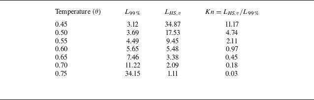
With the liquid–vapour interface resolved, the natural scale of resolution is the thickness of the interface, which, e.g. can be defined as the distance of locations where in an equilibrium state the local density differs by more than 1 % from the saturation densities in either the liquid or the vapour (99 % thickness
 $L_{99\,\%}$
). Data in table 1 show that the 99 % thickness increases with temperature, and assumes values approximately between
 $5$
and
 $30$
particle diameters.
Values of
 $L_{{\textit{HS}},v}$
, the hard-sphere mfp of the saturated vapour phase, 99 % interface thickness
 $L_{99\,\%}$
and Knudsen number
 ${Kn}$
for different dimensionless temperatures
 $\theta$
. The suffix
 ${\textit{HS}},v$
denotes hard-sphere saturated vapour.

The mean free path (mfp) of the (saturated) vapour phase can be estimated from the well-known textbook result
 $L_{{\textit{HS}},v}= {1}/{\sqrt {2}\pi a^{2}(\rho/m)}= {1}/{\sqrt {2}\pi \rho _v^{\textit{sat}}(\theta )}$
(Struchtrup Reference Struchtrup2005; Kremer Reference Kremer2010) (the units are chosen for convenience to be
 $a=m=1$
), which is a decreasing function of temperature with values in table 1 from approximately
 $35$
at
 $\theta =0.45$
to
 $1$
close to the critical temperature.
Small Knudsen numbers imply dominance of local behaviour, while larger Knudsen numbers indicate that non-locality affects transport behaviour. With these values, the vapour mean path is larger than, or comparable to, the interface thickness for a large range of temperatures, and apart from states close to critical, the corresponding Knudsen number is never sufficiently small to warrant a Chapman–Enskog expansion. We must conclude that interface resistance is affected by non-localities that cannot be captured by the NSF equations, which predict a continuous and monotonic change of viscosity and heat conductivity from liquid to vapour.
The typical approach in macroscopic modelling is to consider higher-order moments which allow us to capture non-local transport effects (Torrilhon Reference Torrilhon2016). This was attempted in Struchtrup & Frezzotti (Reference Struchtrup and Frezzotti2022) and Struchtrup et al. (Reference Struchtrup, Jahandideh, Couteau and Frezzotti2024) with mixed results. It was shown that the NSF framework, when used with transport coefficients obtained via the Chapman–Enskog expansion, severely underestimates interfacial resistance, while models with higher moments overestimate resistance. Thus, it appears rather difficult to develop a physical model – that is, an approximation to the EV equation – that accurately captures the complicated processes within the interface.
We are interested in a NSF model for the bulk phases with a meaningful description of the interface, so that agreement with solutions of the EV equation is sufficiently good. As the comparison of solutions of the original EV-NSF equations and the EV equation shows, the NSF model underestimates interface resistance, so that, e.g. temperature jumps are too small. In the light of the above discussion of Knudsen numbers, this failure of the NSF equations must be attributed to its inability to account for non-local effects.
The proposed correction of the NSF model increases resistance in the interface such that agreement with solutions of the EV equation is acceptable. The corrected model thus mixes physical modelling, i.e. equations and transport coefficients derived from the EV equation, with phenomenological modelling, where transport coefficients are fitted to accurate EV data.
This interpretation is further supported by the fact that the steep density variation across only a few particle diameters in the interface prevents the use of classical continuum arguments based on short mfps. Solutions of the EV equations yield larger temperature jumps and pressure deviations that cannot be described by the NSF equations, unless one corrects the transport coefficients. The observed larger jumps indicate larger interface resistance than expected from NSF, and agreement can be obtained by decreasing viscosity and heat conductivity within the interfacial zone. Thus, the dip observed in figure 6 should not be viewed as unphysical, but rather as the macroscopic representation of the enhanced interfacial resistance captured by kinetic theory.
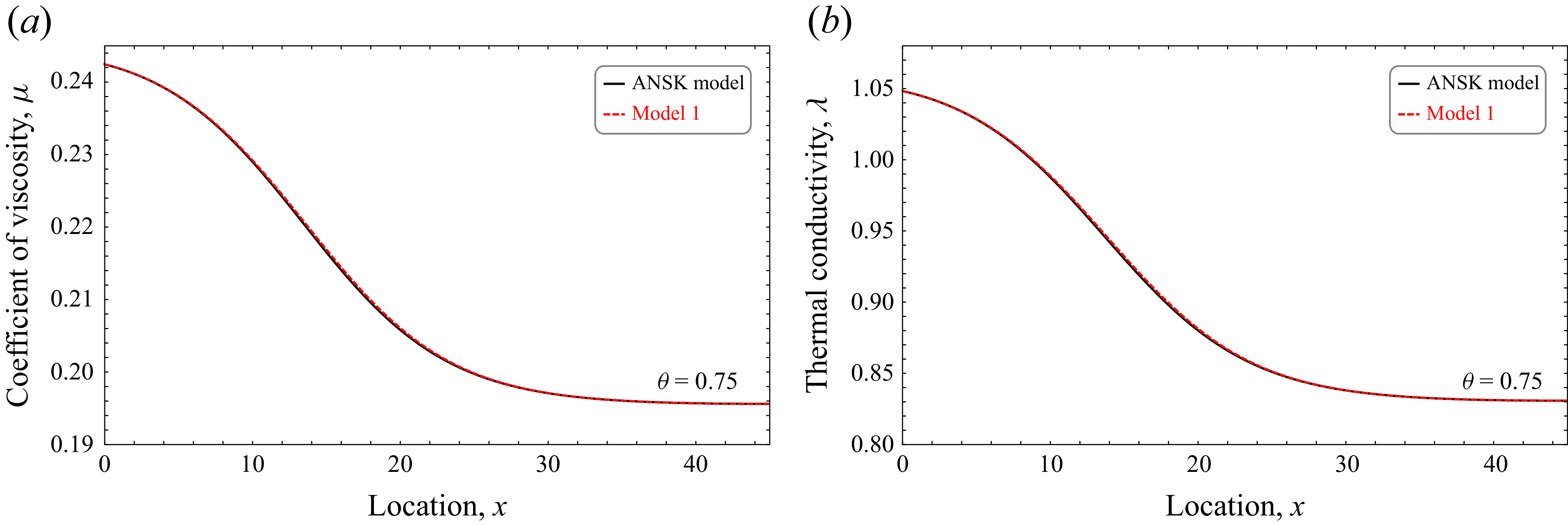
Comparison of coefficient of viscosity (a) and thermal conductivity (b) computed from ANSK model (black solid line) and model 1 (red dashed line) for
 $\theta = 0.75$
.

Additional evidence for this interpretation comes from the behaviour near the critical point. Figure 8 shows the viscosity and thermal-conductivity profiles at
 $\theta = 0.75$
, for which the Knudsen number is
 ${Kn} = 0.03$
(see table 1). At this temperature, the mfp becomes much smaller than the interface thickness, indicating that non-local effects are negligible and transport is dominated by local continuum behaviour. Consistent with this expectation, the dip observed in figure 6 at lower temperatures disappears entirely, and both transport coefficients vary smoothly and monotonically across the interface. This confirms that the localised reduction in transport coefficients at subcritical temperatures originates from non-local effects rather than from an unphysical artefact of the model. As the Knudsen number decreases toward the critical point, the ANSK model naturally recovers the NSF-like monotonic behaviour, thereby demonstrating that the observed dips are a genuine reflection of enhanced interfacial resistance induced by non-locality.
Overall, the ANSK model incorporating this correction shows excellent agreement with the full EV model and MD simulations, especially in capturing interfacial features. This agreement supports the appropriateness of including gradient-dependent modifications in transport properties for nanoscale systems.
4.3. One-dimensional steady-state heat transfer without phase change
Next, we consider steady-state, one-dimensional heat transfer across a liquid–vapour interface without phase change (
 $J=0$
), where
 $J$
denotes the total mass flux. The domain
 $x \in [0, L]$
is discretised with a uniform grid spacing, with the interface located at
 $x = L_0$
. At the liquid boundary (
 $x=0$
), a constant mass flux
 $J$
and the temperature
 $\theta _l$
are imposed, while at the vapour boundary (
 $x=L$
), either the vapour temperature
 $\theta _v$
is prescribed or, under adiabatic conditions, the temperature gradient – and thus the heat flux
 $q_V$
– is set to zero, following Struchtrup et al. (Reference Struchtrup, Jahandideh, Couteau and Frezzotti2024). The non-zero variables are {
 $\rho (x),q_{x}(x)={q}(x)$
}.
Governing equations: Conservation laws for this case now reduce to
 \begin{align} J = \rho v = 0, \quad \frac {{\textrm d}}{{\textrm d}x} \left [\rho \theta + \frac {2\pi }{3} \rho ^{2} \theta Y + \tau _{xx}^K\right ] = 0, \quad -\lambda \frac {{\textrm d}\theta }{{\textrm d}x} = q_c = \text{constant}, \end{align}
where
 $\tau _{xx}^{K}$
is the one-dimensional Korteweg stress component capturing capillarity effects. We solve (4.5) using a fourth-order finite difference scheme on a uniform grid with
 $2n$
points, incorporating the boundary conditions and an appropriate initial guess for both density and temperature profiles, as outlined by Struchtrup et al. (Reference Struchtrup, Jahandideh, Couteau and Frezzotti2024). The resulting
 $2n+1$
nonlinear equations are then solved using the fsolve command in
 $\textrm {MATLAB}^{\circledR }$
.
The divergence of the Korteweg stress tensor in (3.1), introduces third-order spatial derivatives in (4.5), which require careful numerical treatment. In our simulations, we use a fourth-order central finite difference scheme on a uniform grid to evaluate all spatial derivatives. This approach provides high accuracy, particularly across the narrow interfacial region where density changes from liquid to vapour over a distance of 10–20 molecular distances. Since the study focuses on steady-state problems, time integration is avoided. Instead, the resulting system of nonlinear algebraic equations is solved using the fsolve command in
 $\textrm {MATLAB}^{\circledR }$
. The grid resolution is chosen such that the interface is resolved with at least 20–30 points. Typical simulations use
 $n = 1200$
–2200 grid points over domains of size
 $L = 120$
–220, depending on the specific problem configuration.
Comparison of density and temperature from the ANSK model (black solid line), EV-DSMC (black diamonds) and model 1 (red dashed line) for three non-evaporative heat transfer cases. Rows: (a,b)
 $L=200$
,
 $\theta _l=0.65$
,
 $\theta _v=0.70$
,
 $\alpha = 2.4$
,
 $q_{c} = -1.90 \times 10^{-4}$
; (c,d)
 $L=120$
,
 $\theta _l=0.60$
,
 $\theta _v=0.64$
,
 $\alpha = 1.83$
,
 $q_{c} = -1.55 \times 10^{-4}$
; (e,f)
 $L=220$
,
 $\theta _l=0.52$
,
 $\theta _v=0.60$
,
 $\alpha = 0.69$
,
 $q_{c} = -1.99 \times 10^{-4}$
; with
 $L_0=40$
,
 $J=0$
.

4.3.1. Results and discussion
Figure 9 shows density and temperature profiles for different boundary temperatures. The ANSK model (black solid line) shows excellent agreement with EV-DSMC data (black diamonds) (Struchtrup et al. Reference Struchtrup, Jahandideh, Couteau and Frezzotti2024), validating the role of the temperature-dependent capillarity coefficient
 $\chi _3(\theta )$
(Bhattacharjee et al. Reference Bhattacharjee, Struchtrup and Singh Rana2024b
) and gradient-dependent thermal conductivity
 $\lambda (\rho , \boldsymbol{\nabla }\rho )$
(Bedeaux et al. Reference Bedeaux, Johannessen and Røsjorde2003; Johannessen & Bedeaux Reference Johannessen and Bedeaux2004). Model 1 (
 $\alpha = 0$
), which basically represents the classical NSK equations, agrees well for the density profiles but fails to capture interfacial behaviour and predicts a flat interface for the temperature plots (red dashed line).
The transport coefficients employed in this study are initially derived from the EV equation and subsequently corrected in the interfacial region through comparison with DSMC results based on the Sutherland potential. For more realistic fluids, such as those modelled with the Lennard–Jones potential, these coefficients require adjustment, as done in (Homes et al. Reference Homes, Frezzotti, Nitzke, Struchtrup and Vrabec2025). To further evaluate the validity of the model, we compare our solution for one-dimensional, non-evaporative heat transfer with MD simulation results reported by Homes et al. (Reference Homes, Frezzotti, Nitzke, Struchtrup and Vrabec2025). In that study, the MD results were transformed for comparison with DSMC data, as detailed in the paper Homes et al. (Reference Homes, Frezzotti, Nitzke, Struchtrup and Vrabec2025), and our results show good agreement with the transformed MD data.
Although the mfp is large in both the vapour phase and the interfacial region, the impact of non-locality on macroscopic transport is fundamentally different in these two settings. In the vapour bulk, the density is nearly uniform and the temperature and velocity profiles remain almost linear, so particles typically traverse their full mfp without encountering strong spatial variations. Under such conditions, the classical NSF constitutive laws remain accurate, as is also observed in standard rarefied-gas flows outside the thin Knudsen boundary layers.
In contrast, the liquid–vapour interface contains very steep density gradients over distances comparable to, or smaller than, the local mfp. This sharply reduces the effective free-travel distance of particles, increases the local collision rate and enhances the influence of the mean-field (Vlasov) forces. As a result, the macroscopic heat and momentum fluxes deviate from the NSF form, and the effective transport coefficients within the interface become smaller than their bulk Enskog values, despite the fact that the underlying microscopic (collisional) coefficients are unchanged.
These observations explain why a change to the classical NSF constitutive laws is needed only in the interfacial region. The strong density gradients there introduce non-local effects that cause the macroscopic fluxes to deviate from the NSF form, even though the underlying Enskog transport coefficients themselves do not change. The gradient-dependent correction offers a practical way to represent this interfacial behaviour within a continuum model, while the vapour phase continues to be well described by the standard NSF relations.
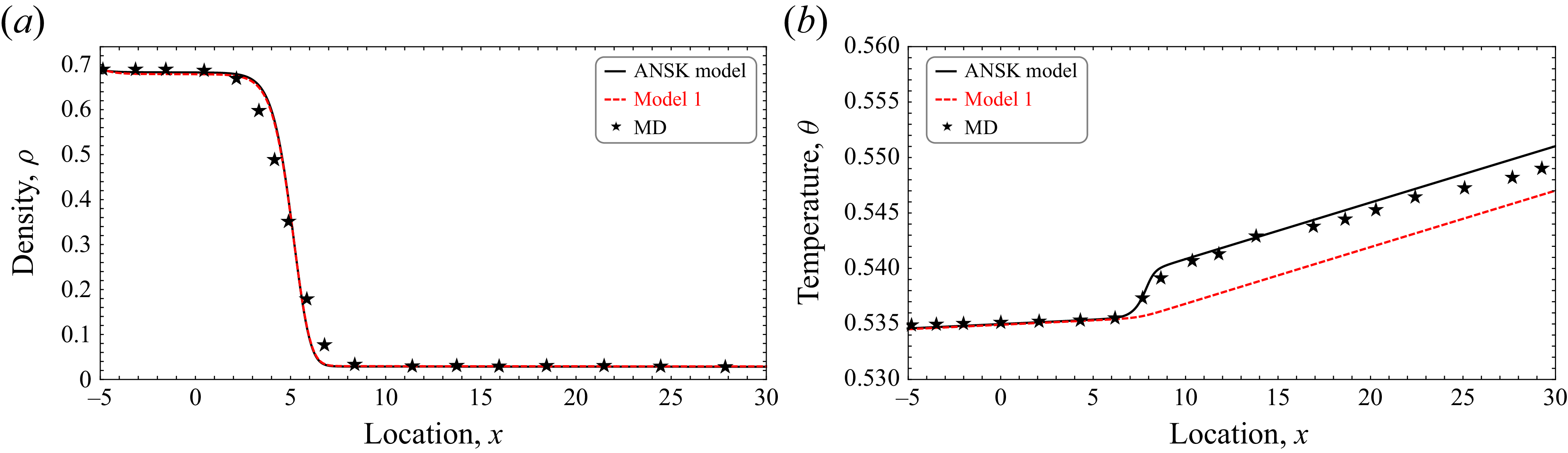
(a) Comparison of density and (b) temperature profiles from the ANSK model (black solid line), model 1 (red dashed line) and MD simulations (black stars) for non-evaporative heat transfer case. Here,
 $\theta _l=0.5348$
,
 $\alpha = 0.52$
and
 $q_{c} = -2.55 \times 10^{-4}$
.

4.4. Validation against molecular dynamics simulations
The results depicted by the black solid line in figure 10 represent the solution obtained from the ANSK model, while the red dashed line corresponds to model 1 with
 $\alpha = 0$
, and the black stars denote MD simulation data reported in Homes et al. (Reference Homes, Frezzotti, Nitzke, Struchtrup and Vrabec2025). The ANSK model results shown here are computed at
 $\theta _{l} = 0.5348$
(liquid bulk temperature) and
 $q_c = -2.55 \times 10^{-4}$
, with the parameter
 $\alpha = 0.52$
, which is determined phenomenologically in this case to match the MD simulation results. While the ANSK model has been validated against the EV kinetic equation throughout in this study, originally designed for dense hard-sphere fluids, this comparison is intended to further evaluate the model’s accuracy by benchmarking it against MD simulations based on realistic interaction potentials.
The comparison shows that both the ANSK model and model 1 provide density profiles that align well with the MD simulation results. However, a clear difference emerges in the temperature predictions. The ANSK model accurately captures the interfacial temperature variation and shows excellent agreement with the MD data. In contrast, model 1 fails to resolve the interfacial structure and instead predicts a nearly flat temperature profile in this region. This discrepancy highlights the limitation of relying on transport coefficients that depend only on the local density. By incorporating density-gradient-dependent transport coefficients – particularly for thermal conductivity – the ANSK model introduces additional thermal resistance near the interface. This allows it to better resolve the temperature gradients observed in the MD simulations. These results underscore the importance of including non-local effects in continuum models when modelling heat transfer at nanoscales.
4.5. One-dimensional steady state with forced evaporation
Evaporation strongly influences interfacial heat and mass transport. Following Struchtrup et al. (Reference Struchtrup, Jahandideh, Couteau and Frezzotti2024), we consider zero heat flux in the vapour bulk (
 $q_{{V}}$
). The non-zero fields for this one-dimensional problem with forced evaporation are {
 $\rho (x),\, v_{y}(x)=v_{y},\, \sigma _{xy}(x)=\sigma (x),\, {q_{x}}(x)={q(x)}$
}.
Governing equations: conservation laws for the case with forced evaporation reduce to
 \begin{equation} \rho v = J = \text{constant},\quad\!\! \frac {{\textrm d}}{{\textrm d}x} \left (\rho v_{y}^{2} + {\varPi _{x}}\!\right ) = 0,\quad\!\! \frac {{\textrm d}}{{\textrm d}x}\left [ \left ( \frac {3}{2} \rho \theta + \frac {1}{2} \rho v_{y}^2 + \rho \varepsilon _{K,x} \!\right ) v_{y} + \mathcal{J}_{x}\right ] = 0, \end{equation}
where
 $\varPi _x$
,
 $\varepsilon _{K,x}$
and
 $\mathcal{J}_x$
denote the
 $x$
-components, in the one-dimensional setting, of the total momentum flux tensor, non-local potential energy and energy flux vector as defined above.
Equations (4.6) are solved using the numerical method outlined in (4.3), with boundary conditions at both the left and right boundaries specified based on the EV-DSMC data. These boundary conditions are then used to solve the NSK equations in the bulk, with the resulting solutions serving as initial guess profiles for the equations in (4.6).
4.5.1. Results and discussion
Figure 11(a,c) shows the density and temperature Figure 11(b,d) profiles for two evaporation cases, with
 $L_0 = 60$
, and
 $q_{{V}} = 0$
. Figure 11(a,b)
 $\theta _l = 0.60$
,
 $\theta _v = 0.56$
,
 $J = 0.000745$
,
 $\alpha = 1.26$
; Figure 11(c,d)
 $\theta _l = 0.52$
,
 $\theta _v = 0.48$
,
 $J = 0.00035$
,
 $\alpha = 0.31$
. The ANSK model (black solid lines) agrees closely with EV-DSMC results (black diamonds) (Struchtrup et al. Reference Struchtrup, Jahandideh, Couteau and Frezzotti2024), for both the density and temperature profile. Model 2 results coincides with the ANSK model showing negligible role of stress gradient in heat transfer problems.
Based on the assigned mass flux
 $ J = \rho v$
and the computed boundary values of density, the evaporative velocities at the domain boundaries in figure 11 indicate that the system operates in a weak evaporation regime. Specifically, the velocities at the liquid boundary range from
 $ 4.87 \times 10^{-4}$
to
 $ 1.21 \times 10^{-3}$
, while on the vapour side, they reach up to
 $ 2.80 \times 10^{-2}$
. Across all cases considered, the maximum evaporative velocity reliably simulated with the present model is
 $ 0.1235$
.
Density and temperature profiles with forced evaporation, comparing the ANSK model, EV-DSMC, model 1 and model 2. (a–b)
 $L = 200$
,
 $\theta _l = 0.60$
,
 $\theta _v = 0.56$
,
 $J = 0.000745$
,
 $\alpha = 1.26$
. (c–d)
 $L = 220$
,
 $\theta _l = 0.52$
,
 $\theta _v = 0.48$
,
 $J = 0.00035$
,
 $\alpha = 0.31$
. Interface at
 $L_0 = 60$
.

Temperature jump across the interface, defined as
 $ \theta _l - \theta _v$
, plotted as a function of the Mach number.

To further examine the applicability range of the ANSK model under increasing non-equilibrium conditions, simulations were performed to examine the temperature jump across the interface, defined as
 $\theta _{l}-\theta _{v}$
, as a function of the Mach number
 $Ma$
, given by
 \begin{align} {Ma} = \frac {v_{0}}{\sqrt {\dfrac {5}{3} \theta _{0}}}, \end{align}
where
 $v_{0}$
denotes the far-field vapour velocity and
 $\theta _{0}$
is the reference temperature. As shown in figure 12, the temperature jump increases linearly with
 $Ma$
, consistent with expectations in the low Mach number regime
 $(Ma\lt 0.1)$
where the dynamics remains effectively linear. The ANSK model yields converged and physically consistent solutions up to a maximum Mach number of approximately 0.1381. Beyond this point, the numerical method – based on nonlinear root-finding algorithm (MATLAB®’s fsolve) – fails to converge. This indicates that the current approach is suitable for weak to moderately strong evaporation regimes, but for higher Mach numbers, more robust numerical schemes such as finite volume methods may be necessary to capture the nonlinearities and ensure convergence.
5. Conclusion
This work presents a thermodynamically consistent extension of the classical NSK model, systematically derived from the EV kinetic equation to accurately capture interfacial transport processes at the nanoscale. While the classical NSK equations assume local equilibrium and density-dependent transport properties (see (3.5) and (3.6)) – assumptions that break down in regions with steep gradients and strong non-equilibrium effects – the proposed model incorporates microscopic physics through a continuum framework. This makes it suitable for simulating dense fluids and multiphase systems where classical formulations fall short. Validation against DSMC for the EV equation across three benchmark problems – two-phase Couette flow, non-evaporative heat conduction and planar evaporation – demonstrates that the ANSK model achieves close agreement with kinetic theory predictions. In particular, the inclusion of a temperature-dependent Korteweg coefficient, density gradient-dependent transport coefficient and a temperature-dependent parameter
 $\alpha$
in the ANSK model significantly improves the model’s accuracy in capturing the interfacial dynamics, without compromising computational efficiency. Moreover, the model adheres to the second law of thermodynamics, as confirmed through a detailed entropy production analysis.
Overall, this study bridges the gap between computationally expensive kinetic theory models and continuum-based approaches, offering a robust framework for applications in nanoscale thermal management, phase-change heat transfer and microfluidic systems.
Despite its strengths, the ANSK model is inherently limited by its five-moment formulation, which includes only mass, momentum and energy conservation. The absence of separate evolution equations for stress and heat flux restricts its ability to resolve non-equilibrium phenomena such as Knudsen layers and other non-equilibrium effects. Capturing these effects would require a more detailed description of the distribution function, for example via higher-order moment approximations, which is only accessible through kinetic models or extended moment closures like the regularised 13-moment equations (Struchtrup & Torrilhon Reference Struchtrup and Torrilhon2003; Rana et al. Reference Rana, Gupta, Sprittles and Torrilhon2021).
Future extensions of this work will address several of these limitations. For example, although the spatial domain in our simulations is non-dimensionalised using the molecular diameter
 $ a$
, the model can be scaled to larger physical domains of the order of hundreds or thousands of nanometres. In dense fluids, where the mfp
 $ \lambda$
remains small, an increase in domain size
 $ L$
leads to a lower Knudsen number
 $ \textrm{Kn} = \lambda / L$
, thereby reinforcing the applicability of continuum assumptions. Accurate resolution of interfacial gradients in such extended domains may require finer grids or adaptive meshing, which we intend to pursue in future work, particularly for applications such as thin-film evaporation and microscale heat transport.
Furthermore, while the model performs well in weak to moderately strong evaporation regimes, it remains to be seen how the model performs in the strong evaporation case. Most importantly, to improve accuracy in capturing effects such as parallel heat flux in Couette flow – where deviations from Fourier’s law are observed – more accurate models, as presented in the literature (Struchtrup & Frezzotti Reference Struchtrup and Frezzotti2022), will also be explored. While the present study focuses on one-dimensional configurations, extending the model to more complex geometries – such as sessile droplets or capillary-driven flows – remains an important direction for future research, as these involve additional physical and numerical challenges.
Acknowledgements
H.S. acknowledges support from NSERC (Discovery Grant RGPIN-2022-03188). A.S.R. acknowledges support from SERB, India (MATRICS MTR/2021/000417).
Declaration of interests
The authors declare that they have no known competing financial interests or personal relationships that could have appeared to influence the work reported in this paper.