



1. Introduction
Turbulence is a complex and spatio-temporally chaotic phenomenon, characterised by a huge number of interacting degrees of freedom hierarchically organised across a wide range of spatial and temporal scales (Frisch Reference Frisch1995). A central and longstanding question is whether turbulent flows retain any degree of predictability and, if so, how this predictability varies across scales. This problem traces back to the seminal works of Lorenz (Reference Lorenz1969) and Leith & Kraichnan (Reference Leith and Kraichnan1972), which established that the nonlinear amplification of the initial perturbation produces an inverse error cascade, whereby small-scale perturbations progressively grow and propagate towards larger scales, ultimately degrading predictability across the entire flow (see Boffetta et al. Reference Boffetta, Celani, Crisanti and Vulpiani1997; Rotunno & Snyder Reference Rotunno and Snyder2008; Boffetta & Musacchio Reference Boffetta and Musacchio2017; Ge et al. Reference Ge, Rolland and Vassilicos2023).
This idea of the error cascade in turbulence has some controversial aspects nonetheless. In particular, one can expect that a small perturbation localised in the viscous scales will be dissipated before it propagates to larger scales. Indeed, recent works questioned the very idea of the butterfly effect in dissipative multiscale systems (Pielke et al. Reference Pielke, Shen and Zeng2024). Surprisingly, despite the conceptual and practical relevance of the problem (Dubrulle et al. Reference Dubrulle, Barlet, Barral, Cheminet, Costa, Dragoni, Harikrishnan, Lopez, Mallick and Pikeroen2025), very few studies have been devoted to studying the evolution of a small and spatially localised perturbation in turbulent flows (Encinar Reference Encinar2024; Powdel & Ray Reference Powdel and Ray2026).
In this letter, we address this problem within a simple but relevant geophysical model given by the surface quasi-geostrophic (SQG) equation. The SQG model describes the advection of the surface potential temperature in a strongly stratified and rotating environment (Held et al. Reference Held, Pierrehumbert, Garner and Swanson1995; Lapeyre Reference Lapeyre2017). In spite of its relative simplicity, the SQG model displays a rich phenomenology with formal analogies with both two- and three-dimensional Navier–Stokes turbulence, as discussed in Valade et al. (Reference Valade, Thalabard and Bec2024). Moreover, SQG dynamics has been used to address the predictability problem and the error cascade to large scales in several studies with the aim of generalising the original analysis by Lorenz (Rotunno & Snyder Reference Rotunno and Snyder2008; Durran & Gingrich Reference Durran and Gingrich2014; Palmer et al. Reference Palmer, Döring and Seregin2014). By using high-resolution numerical simulations of the SQG model, we study the initial evolution of a small, localised perturbation of different sizes. We find that, during this initial phase, as the error propagates from the initial scale to the most unstable modes, the magnitude of the perturbation, measured by the energy of the difference field, can decrease in time. We find that the duration of this initial phase is characterised by a large variability, depending on both the initial size of the perturbation and its location in space. In particular, we find that a small perturbation localised inside a vortical structure of the flow is strongly dissipated, leading to a decrease in the error energy for several small-scale times before experiencing the exponential chaotic growth.
2. Surface quasi-geostrophic model and numerical simulations
The SQG model describes the large-scale dynamics of a rapidly rotating, stably stratified flow in terms of a two-dimensional surface buoyancy field
 $\theta (\boldsymbol {x},t)$
(Pierrehumbert et al. Reference Pierrehumbert, Held and Swanson1994; Lapeyre & Klein Reference Lapeyre and Klein2006)
 \begin{equation} \partial _t \theta + \boldsymbol {u} \boldsymbol{\cdot }\boldsymbol{\nabla } \theta = \nu {\nabla} ^2 \theta + \mu {\nabla} ^{-2} \theta + f \ , \end{equation}
where the incompressible velocity field
 $\boldsymbol {u}(\boldsymbol {x},t)$
is given in terms of a streamfunction
 $\psi (\boldsymbol {x},t)$
as
 $\boldsymbol {u}=(-\partial _y \psi ,\partial _x \psi )$
and,
 $f(\boldsymbol {x},t)$
is a random forcing, tipically active on a scale
 $\ell_f$
. The relation between the buoyancy field and the streamfunction is formally
 $\psi =|\boldsymbol{\nabla }|^{-1} \theta$
or, in Fourier space,
 $\hat {\psi }=\hat {\theta }/k$
, where
 $k=|\boldsymbol {k}|$
is the modulus of the wavenumber
 $\boldsymbol {k}$
. The dissipative terms in the SQG model represent the effects of scales not resolved by the model, their specific form being somewhat arbitrary (see Lapeyre & Klein Reference Lapeyre and Klein2006). In (2.1) we introduce a diffusivity
 $\nu$
and a large-scale damping
 $\mu$
chosen to be active at, respectively, small and large scales.
In the absence of forcing and dissipation, the dynamics (2.1) conserves two invariants, the vertically integrated energy (VIE)
 $V=\langle \psi \theta \rangle _x/2$
, which is the SQG analogue of the total energy of the associated three-dimensional quasi-geostrophic flow, and the surface potential energy (SPE)
 $E=\langle \theta ^2 \rangle _x/2$
, which measures the variance of the surface buoyancy field. Brackets
 $\langle \ldots \rangle _{x}$
indicate the average over the physical domain. A peculiarity of the SQG model is that, because of the relation between surface buoyancy and velocity, the SPE is also equal to the surface kinetic energy, i.e.
 $\langle \theta ^2 \rangle _x = \langle |\boldsymbol{u}|^2 \rangle _x$
.
In forced-dissipative SQG turbulence, these two inviscid invariants are transferred in opposite directions. The SPE undergoes a direct cascade towards small scales, where it is removed by the diffusive term
 $\nu {\nabla} ^2\theta$
. The VIE undergoes an inverse cascade towards large scales, where it is removed by the large-scale friction term
 $\mu {\nabla} ^{-2}\theta$
. The viscous and friction terms therefore provide, respectively, the small-scale and large-scale cutoffs required to obtain a statistically stationary state.
In the turbulent regime, the SQG flow produces a direct cascade of SPE à la Kolmogorov with an SPE spectrum, or energy spectrum close to the dimensional prediction (Pierrehumbert et al. Reference Pierrehumbert, Held and Swanson1994)
 \begin{equation} E(k) \simeq \varepsilon ^{2/3} k^{-5/3} \end{equation}
in the range of wavenumbers
 $1/\ell _{\!f} \ll k \ll 1/\ell _{\nu }$
, where
 $\ell _{\nu }=(\nu ^3/\varepsilon )^{1/4}$
is the diffusive (Kolmogorov) small scale and
 $\varepsilon$
is the average SPE viscous dissipation rate,
 $\varepsilon =\nu \langle |\boldsymbol{\nabla }\theta |^2\rangle _{x,t}$
.
We remark that the scaling (2.2) is not exact, as the direct cascade in SQG displays intermittency corrections, similarly to three-dimensional Navier–Stokes turbulence (Valade et al. Reference Valade, Bec and Thalabard2025). Since the effects of these corrections are relatively small for low-order observables, such as the energy spectrum, they will not be considered in this study.
We perform numerical simulations of (2.1) in a square box of size
 $L=2\pi$
with periodic boundary conditions at resolution
 $8192^2$
and three different Reynolds numbers
 $\textit{Re}=\varepsilon ^{1/3}\ell _{\!f}^{4/3}/\nu$
(see Valadão et al. Reference Valadão, Boffetta, De Lillo, Musacchio and Crialesi-Esposito2025a
for details on the implementation of the code). In all the simulations, the dissipative scale is well resolved as the maximum wavenumber
 $k_{\textit{max}}$
satisfies
 $k_{\textit{max}} \ell _{\nu } \ge 3.0$
. After a transient, the system reaches a statistically stationary turbulent state characterised by a well-developed Kolmogorov spectrum (2.2). In these conditions, we computed the leading Lyapunov exponent
 $\lambda$
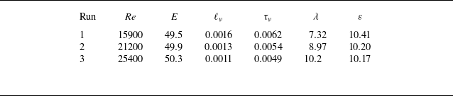
by measuring the rate of logarithmic divergence of two close realisations averaged over a very long trajectory, a standard method in the study of dynamical systems (Cencini et al. Reference Cencini, Cecconi and Vulpiani2009). For the simulations at different Reynolds numbers see table 1, which reports the main properties of the turbulent flow (see Valadão et al. Reference Valadão, De Lillo, Musacchio and Boffetta2025b
for more details).
Parameters of the simulations. The forcing scale is kept constant throughout the simulations:
 $\ell _{\!f}\approx 1.8$
. The typical time scale at the forcing scale is given by
 $\tau _{\!f}=\varepsilon ^{-1/3}\ell _{\!f}^{2/3}\approx 0.68$
. The amplitude
 $\delta _0$
is fixed by the requirement on the initial error energy
 $E_\varDelta (0)=5\times 10^{-9}$
.

Table 1. Long description
A table with three rows and seven columns comparing properties of turbulent flow across three different Reynolds numbers. The columns are labeled Run, Re, E, l#x005F;v, τ#x005F;v, λ, and ε. The rows present the following data: Row 1: Run 1, Re 15900, E 49.5, l#x005F;v 0.0016, τ#x005F;v 0.0062, λ 7.32, ε 10.41. Row 2: Run 2, Re 21200, E 49.9, l#x005F;v 0.0013, τ#x005F;v 0.0054, λ 8.97, ε 10.20. Row 3: Run 3, Re 25400, E 50.3, l#x005F;v 0.0011, τ#x005F;v 0.0049, λ 10.2, ε 10.17.
In the stationary turbulent conditions, at time
 $t=t_0$
we locally modify the reference buoyancy field
 $\theta (\boldsymbol {x},t_0)$
around the point
 $\boldsymbol {x}_0$
to generate a perturbed field
 $\theta '(\boldsymbol {x},t_0)=\theta (\boldsymbol {x},t_0)+\sqrt {2}\ \delta \theta _0(\boldsymbol {x}-\boldsymbol {x}_0)$
. We remark that we consider a zero-average buoyancy field and therefore also the perturbation has a vanishing average over the domain
 $\langle \delta \theta _0 \rangle _x=0$
. Because of the non-local nature of the model (2.1) (due to the incompressibility of the velocity field), a generic perturbation localised in
 $\theta$
does not correspond to a localised perturbation in the velocity field, producing an almost instantaneous spread of the perturbed field. Nonetheless, it is possible to produce a perturbation localised both in the scalar and velocity fields by the combination of a Gaussian with an algebraic decay in Fourier space. Written for the streamfunction, the perturbation has the form
 $\delta \hat {\psi }_0(\boldsymbol {k};\boldsymbol {x}_0)=\delta _0 e^{-\sigma ^2 k^2 / 2} k^{-\beta } e^{-i\boldsymbol {k}\boldsymbol{\cdot }\boldsymbol {x}_0}$
, for
 $\boldsymbol{k}\neq 0$
, and zero otherwise. We fix the exponent
 $\beta =0.4$
from the request that the perturbations in the velocity and in the scalar fields have the same large-distance asymptotic behaviour (see Appendix A). The amplitude
 $\delta _0$
is sufficiently small to guarantee the evolution of the perturbation in the linear regime. The width
 $\sigma$
of the perturbation is the control parameter that we change, together with the Reynolds number, to investigate the effect of spatial confinement on the evolution of the error.
The two simulations of the reference and perturbed fields are then evolved (with the same realisation of the random forcing) and we compute the time evolution of the difference field
 $\delta \theta (\boldsymbol {x},t)=(\theta '(\boldsymbol {x},t)-\theta (\boldsymbol {x},t))/\sqrt {2}$
whose dynamics, in the linear regime, is ruled by
 \begin{equation} \partial _t \delta \theta + \boldsymbol {u} \boldsymbol{\cdot }\boldsymbol{\nabla } \delta \theta = \nu {\nabla} ^2 \delta \theta + \mu{\nabla} ^{-2} \delta \theta - \delta \boldsymbol {u} \boldsymbol{\cdot }\boldsymbol{\nabla } \theta \, . \end{equation}
The distance between the two realisations of the turbulent flow is quantified by the error energy
 $E_{\varDelta }$
and the error-energy spectrum
 $E_{\varDelta }(k,t)$
 \begin{equation} E_{\varDelta }(t) = \int E_{\varDelta }(k,t) {\rm d}k = {1 \over 2} \langle \delta \theta ^2(\boldsymbol {x},t) \rangle _x \ ,\ \end{equation}
which, according to (2.3), evolves as
 \begin{equation} {{\rm d} E_{\varDelta } \over {\rm d}t} = -\nu \langle (\boldsymbol{\nabla }\delta \theta )^2 \rangle _x - \mu \langle ({\nabla} ^{-1} \delta \theta )^2 \rangle _x - \langle \delta \theta \delta \boldsymbol {u} \boldsymbol{\cdot }\boldsymbol{\nabla } \theta \rangle _x. \end{equation}
We note that, with the above definition for the difference field, one has
 $E_{\varDelta }=E$
for completely uncorrelated fields
 $\theta$
and
 $\theta '$
. The balance equation (2.5) shows that the last term in (2.3) is the one responsible for the error growth, while the dissipative terms, at large and small scales, simply reduce the error.
Figure 1(a) shows a snapshot of a turbulent field
 $\theta (\boldsymbol {x},t)$
together with the location
 $\boldsymbol {x}_0$
of
 $18$
different initial perturbations. To test the variability of local perturbations, we divide the computational box into a
 $3 \times 3$
grid. In each subdomain of the grid, we locate the maximum and minimum of
 $|\theta (\boldsymbol {x})|$
and we initialise the perturbation on these points. As shown in figure 1, maxima (represented by filled circles) are at the centre of the vortices, while minima (plus symbols) are in the background field between the vortices. For each perturbation, we compute the evolution of the difference
 $\delta \theta (\boldsymbol {x},t)$
. Figure 1(b) shows the dispersion of the difference field (plotted above a threshold) after a dimensionless time
 $t \lambda =2$
for the two cases labelled with an orange circle in panel (a). It is evident that, when the perturbation is injected inside a vortex, it remains confined and small, while the spreading is much more effective in the case outside the vortex.
(a) Initial turbulent scalar field at
 $\textit{Re}=25\,400$
with the positions of the
 $18$
initial perturbations located by the maximum (circles) and minimum (crosses) of
 $|\theta (\boldsymbol {x})|$
in a
 $3 \times 3$
division of the domain. (b) Spreading of the perturbation at time
 $t \lambda =2$
in the two cases indicated by an orange circle in the left panel. The regions where the perturbation exceeds the threshold
 $\delta _0=\sqrt {2E_\varDelta (0)}=10^{-4}$
are shown in black/green.

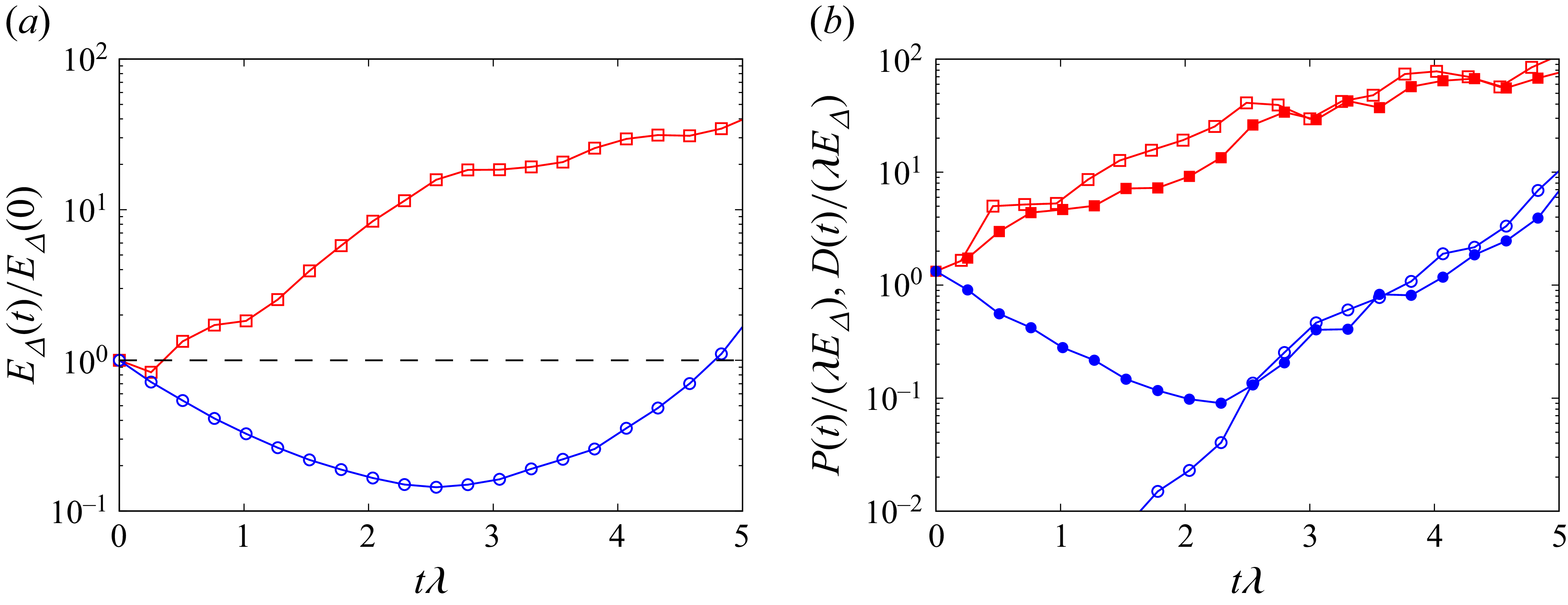
(a) Time evolution of the error energy
 $E_{\varDelta }$
normalised with the initial error for the two cases highlighted in orange in figure 1. Blue circles correspond to the case with the initial perturbation inside a vortex (highlighted circle in figure 1), red squares to the initial perturbation with minimum
 $|\theta (\boldsymbol {x}_0)|$
(highlighted cross in figure 1). (b) Error-energy production term
 $P(t)=-\langle \delta \theta \delta \boldsymbol {u} \boldsymbol{\cdot }\boldsymbol{\nabla } \theta \rangle _x$
(open symbols) and viscous dissipative term
 $\nu \langle (\boldsymbol{\nabla } \delta \theta )^2 \rangle _x$
(filled symbols) normalised with
 $\lambda E_{\varDelta }(0)$
. Blue circles and red squares correspond to the two cases in panel (a).

The time evolution of the error energy for these two cases is shown in figure 2(a). In both cases, we observe an initial decrease of
 $E_{\varDelta }$
due to the dissipation of the perturbation by the diffusive terms (we remark that, by construction, the production term at
 $t=0$
vanishes, as shown in Appendix A). After a transient phase, the error energy starts to increase exponentially, as expected in a chaotic system. Remarkably, we find that the initial decaying phase displays a large variability, which can last several small-scale times, as shown by these two examples (see figure 6 in Appendix B for the evolution of
 $E_{\varDelta }$
on the whole set of 18 simulations).
To better understand the source of this variability, in figure 2(b) we plot the time evolution of the two contributions to the error-energy balance, i.e. the dissipation and the production terms on the right-hand side of (2.5). We see that the production term remains very small for a long time when the perturbation is inside a vortex. This can be understood geometrically from the fact that, in an almost circular vortex,
 $\boldsymbol{\nabla }\theta$
is predominantly radial, while both the perturbation velocity
 $\delta \boldsymbol {u}$
and the velocity field
 $\boldsymbol {u}$
are initially oriented along the azimuthal direction. This local misalignment between
 $\boldsymbol{\nabla }\theta$
and
 $\delta \boldsymbol {u}$
suppresses the initial evolution of the production term in (2.5), while the advection term
 $\boldsymbol {u}\boldsymbol{\cdot }\boldsymbol{\nabla }\delta \theta$
is also reduced. As a result, dissipation dominates the dynamics over a large time interval, delaying the onset of exponential growth.
The observed variability calls for a statistical analysis of the initial decaying phase. With this aim, we define the return time
 $\tau _R$
as the time required for the error energy to recover its initial value,
 $E_{\varDelta }(\tau _R)=E_{\varDelta }(0)$
, and we also compute the minimum value
 $E_{\textit{min}}$
reached by
 $E_{\varDelta }$
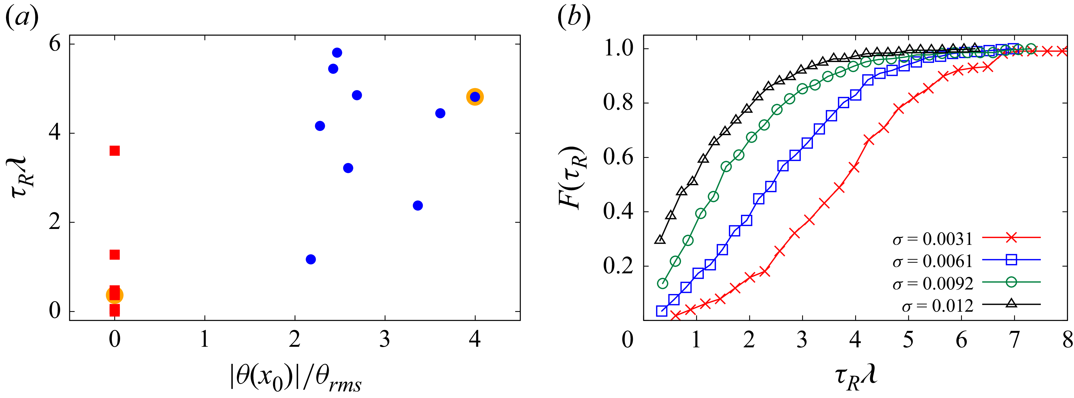
during this time interval. Figure 3(a) shows the return time for the
 $18$
simulations of figure 1(a) as a function of the magnitude of the initial scalar field. A clear tendency toward two groups is observed, associated with perturbations initialised inside (large
 $|\theta (\boldsymbol{x}_0)|$
, circles) or outside (small
 $|\theta (\boldsymbol{x}_0)|$
, squares) coherent vortical structures. In most cases, a small (large) initial value of
 $|\theta (\boldsymbol{x}_0)|/\theta _{\textit{rms}}$
is associated with a short (long) return time, as in the examples of figure 2. Nonetheless, there are a few cases in which this simple correlation fails. This is because
 $\tau _R$
depends not only on the initial local structure of the flow, but also on its subsequent evolution. For instance, in two of the
 $18$
realisations, the vortex initially surrounding the perturbation is rapidly dissipated by the dynamics. Therefore, although
 $|\theta (\boldsymbol{x}_0)|$
provides a useful indicator of the return time, the fate of a localised perturbation cannot in general be inferred from its initial environment alone.
In order to characterise the transient behaviour of the perturbation, we performed a statistical analysis with many (between
 $200$
and
 $300$
) realisations of the initial perturbation placed at random initial positions in the domain. The numerical experiment is then repeated for different sizes
 $\sigma$
of the initial perturbation and for
 $3$
different Reynolds numbers.
(a) Return time as a function of the initial magnitude of the buoyancy field at the perturbation point
 $|\theta (\boldsymbol {x}_0)|$
for the
 $18$
simulations of figure 1. (b) Cumulative distribution function
 $F(\tau _R)$
of the return time
 $\tau _R$
for the simulation at
 $\textit{Re}=15\,900$
and a different initial size of the error. Distributions are computed on many realisations ranging from
 $190$
to
 $375$
from smaller to larger
 $\sigma$
, respectively.

Figure 3. Long description
Panel A: A scatter plot shows the return time (τ#x005F;R λ) on the vertical axis and the initial magnitude of the buoyancy field (|θ(x#x005F;0)|/θ#x005F;rms) on the horizontal axis. The data points are represented by different symbols and colors, indicating varying conditions or simulations. Panel B: A line graph displays the cumulative distribution function F(τ#x005F;R) on the vertical axis and the return time (τ#x005F;R λ) on the horizontal axis. Multiple lines, each represented by different symbols and colors, correspond to different initial sizes of the error (σ). The legend on the right side of the graph indicates the values of σ for each line.
An example of the statistics obtained from these numerical experiments for the case at lower Re is shown in figure 3, where we plot the cumulative distribution function of the return times
 $F(\tau _R)$
for four different values of the perturbation size
 $\sigma$
. It is evident that the return time ranges from a small fraction of
 $\lambda$
to several Lyapunov times and that this variability is more extreme for small perturbations. Moreover, the distribution is shifted to larger values of
 $\tau _R$
for a smaller size of the initial error.
(a) Mean return time
 $\langle \tau _R \rangle$
as a function of the perturbation width
 $\sigma$
for simulations at different Reynolds numbers. (b) Mean return time rescaled with the Lyapunov exponent
 $\lambda$
as a function of the perturbation width
 $\sigma$
made dimensionless with
 $\ell _{\nu }$
. Colours and symbols as in (a). The dashed line represents
 $-1.81 \log (\sigma /\ell _{\nu })+4.78$
. Inset: the minimum error energy normalised with the initial one as a function of perturbation width.

From the distribution shown in figure 3, we compute the mean value of the return times
 $\langle \tau _R \rangle$
, plotted in figure 4(a) as a function of the perturbation width
 $\sigma$
and for the different Reynolds numbers. Figure 4(a) shows that the return time increases for smaller
 $\sigma$
, as expected from figure 3, and decreases by increasing the Reynolds number, i.e. the Lyapunov exponent, of the flow.
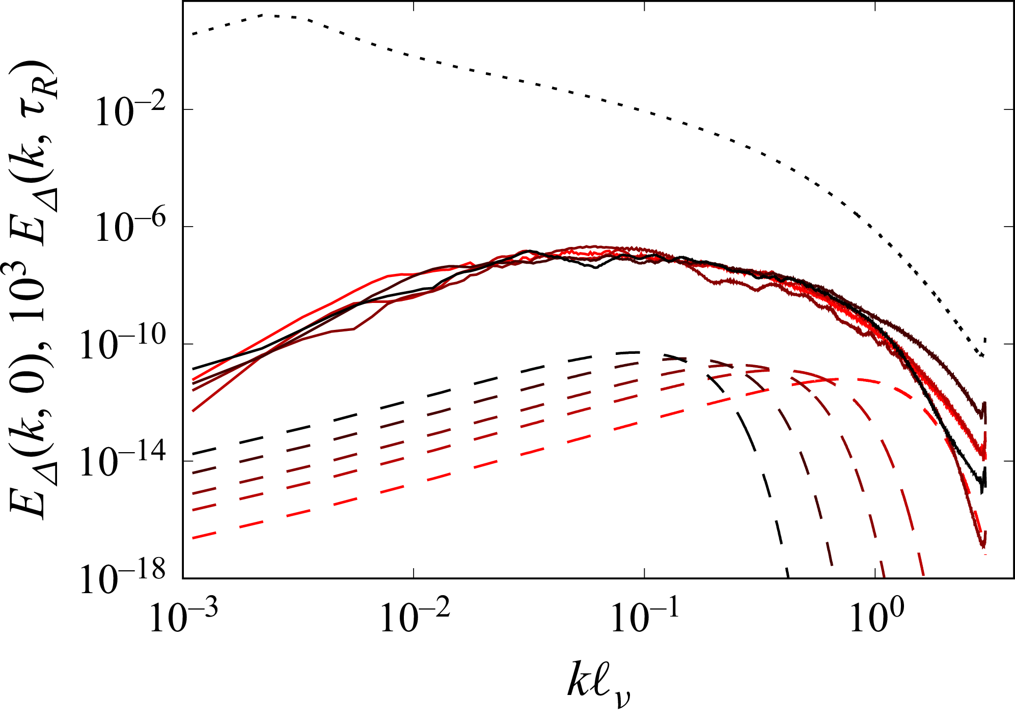
Initial error-energy spectra
 $E_{\varDelta }(k,0)$
(dashed lines) and error-energy spectra at the final time
 $E_{\varDelta }(k,T_{\!f})$
(continuous line) for initial error sizes
 $\sigma =1.4 \ell _\nu$
,
 $\sigma =2.8\ell _\nu$
,
 $\sigma =4.2\ell _\nu$
,
 $\sigma =7.0\ell _\nu$
,
 $\sigma =10.9\ell _\nu$
(from red to black) for run 3. For clarity, the energy spectra at the final time are multiplied by a factor
 $10^3$
. The black dotted line represents the energy spectrum
 $E(k)$
of the field.

In order to understand the dependence of
 $\langle \tau _R \rangle$
on
 $\sigma$
, we consider the error spectra in Fourier space. Figure 5 shows the evolution of the error spectra
 $E_{\Delta }(k,t)$
for the simulation at
 $\textit{Re}=25\,400$
. Initial perturbations at different values of
 $\sigma$
correspond to different initial spectra peaked at wavenumbers
 $k_{\sigma } \propto 1/\sigma$
, shown as dashed lines in figure 5. At the time
 $T_{\!f}$
, when the error energy reaches the value
 $E_{\varDelta }(T_{\!f})=4 E_{\varDelta }(0)$
, the error growth is in the exponential regime and the error-energy spectrum assumes a universal shape peaked at the most unstable wavenumber
 $k_{u}$
, independent of the initial value of
 $\sigma$
. We remark that, as clear from figure 5, we are still in the linear regime in which the error field grows according to (2.3). At longer times, not investigated here, we enter the nonlinear regime in which the error is transferred to larger scales and eventually saturates.
The evolution of the error in Fourier space shown in figure 5 allows us to understand the dependence of
 $\langle \tau _R \rangle$
on
 $\sigma$
by a simple argument based on two modes involved in the process. The first is
 $k_{\sigma }$
, which is the most energetic mode determined by the initial perturbation. The second is the most unstable mode
 $k_u$
, which is known to be around
 $k_u \ell _{\nu } \simeq 0.1$
(Valadão et al. Reference Valadão, De Lillo, Musacchio and Boffetta2025b
). This is the wavenumber at which the error-energy spectrum
 $E_{\varDelta }(k)$
grows exponentially with the Lyapunov exponent of the flow, i.e.
 $E_{\varDelta }(k_u,t) \simeq E_{\varDelta }(k_u,0) e^{2 \lambda t}$
(for simplicity we neglect the fluctuations of the Lyapunov exponent, see e.g. Crisanti et al. Reference Crisanti, Paladin and Vulpiani1988).
For the perturbation with spatial decaying exponent
 $\beta$
concentrated at wavenumber
 $k_{\sigma } \sim 1/\sigma \gg k_u$
, the initial ratio of the energies at the two modes is
 $E_{\varDelta }(k_u,0)/E_{\varDelta }(k_{\sigma },0) \simeq (k_u/k_{\sigma })^{3-2 \beta } \ll 1$
. Since
 $k_{\sigma }$
is in the dissipative range, the corresponding energy is strongly dissipated while the energy at
 $k_u$
grows exponentially. Therefore, the time it takes for the error energy at wavenumber
 $k_u$
to reach the initial value can be estimated from the condition
 $(k_u/k_{\sigma })^{3-2 \beta } e^{2 \lambda \tau _R} = 1$
, which means
 $\tau _R \simeq -(C/\lambda )\log (\sigma /\ell _\nu )$
, where
 $C$
is a constant which depends on
 $\beta$
. Figure 4(b) shows that this prediction works very well when we rescale the mean return time with the Lyapunov exponent of the flow and
 $\sigma$
with the dissipative scale
 $\ell _\nu$
. The inset of figure 4(b) shows the minimum value
 $E_{min}$
reached by the error energy normalised with the initial error. When
 $\sigma /\ell _\nu \ge 10$
the minimum disappears since
 $\tau _R \to 0$
.
3. Discussion and conclusions
We studied the butterfly effect in the forced-dissipative SQG turbulence, a classical two-dimensional model for geophysical flows which has many analogies with the three-dimensional Navier–Stokes equations. By perturbing the turbulent flow with a small perturbation localised in space, we find that exponential amplification of the perturbation is preceded by a pre-asymptotic stage, during which the spectrum of the perturbation aligns with the most unstable wavenumber and the energy of the error field decreases in time.
We study the statistics of this initial phase, and we find that its duration, the return time, is characterised by a large variability depending on the local properties of the turbulent flow at the position of the initial perturbation. The average return time depends logarithmically on the scale of the perturbation, and this dependence can be heuristically understood as the result of a competition between two scales: the injection scale of the perturbation, which decays, and the most unstable scale of the flow, which grows exponentially.
Space–time intermittency is associated with the long-lived large-scale coherent structures observed in SQG turbulence (Valadão et al. Reference Valadão, Ceccotti, Boffetta and Musacchio2024, Reference Valadão, De Lillo, Musacchio and Boffetta2025b ). We have seen that when the initial perturbation is localised inside a vortex, the return time is typically large, but there are exceptions, and the fate of the perturbation does not depend only on the local magnitude of the scalar field. A more complete characterisation of the conditions necessary to achieve long predictability with localised perturbations is left for future investigations. We also remark that the observed transient behaviour depends on the norm used to measure the trajectory separation. While the energy norm (2.4) is a natural one, other choices are possible, and we expect that the quantitative behaviour observed during the initial transient depends on the norm chosen.
The central question behind the real butterfly effect, i.e. whether a small localised perturbation is ultimately absorbed by the dissipative nature of real turbulent flows, cannot ignore the role of small-scale noise (Thalabard et al. Reference Thalabard, Bec and Mailybaev2020; Bandak et al. Reference Bandak, Mailybaev, Eyink and Goldenfeld2024). From a conceptual point of view, when a small perturbation in the dissipative range initially decays, it can reach very small scales and amplitudes where the role of thermal noise cannot be neglected. While this effect is irrelevant in the present SQG model – where viscous dissipation represents a parametrisation of unresolved smaller scales – it is expected to play a role in three-dimensional Navier–Stokes turbulence, where molecular viscosity is explicitly resolved. It would therefore be very interesting to study the effects of thermal noise on an initially small perturbation in conditions accessible to laboratory experiments.
Acknowledgements
We acknowledge HPC CINECA for computing resources within the grants INFN25-FieldTurb and INFN26-FieldTurb. We are indebted to A. Vulpiani for the inspiration behind this work.
Funding
V. J. V. acknowledges the support by the Italian Ministry of University and Research (MUR) - Fondo Italiano per la Scienza (FIS2) - 2023 Call, project DeepFL, CUP: E53C24003760001.
Declaration of interests
The authors report no conflict of interest.
Data availability statement
Data are available upon request.
Appendix A. The localised perturbation
In this appendix, we discuss the shape of the localised perturbation used in the simulations. For simplicity, we set
 $\boldsymbol {x}_0=0$
; the dependence on
 $\boldsymbol {x}_0$
is recovered by the phase factor
 $e^{-i\boldsymbol {k}\boldsymbol{\cdot }\boldsymbol {x}_0}$
in Fourier space. The perturbation is prescribed for the streamfunction as
 \begin{equation} \delta \hat \psi _0(k) = A e^{-\sigma ^2 k^2/2} k^{-\beta }. \end{equation}
The perturbation is radially symmetric in physical space. Therefore, its inverse Fourier transforms can be written as Hankel transforms. Thus, we can write the streamfunction as
 \begin{equation} \delta \psi _0(r) = \frac {A}{2\pi } \int _0^\infty k^{1-\beta } e^{-\sigma ^2 k^2/2} J_0(kr)\,{\rm d}k , \end{equation}
where
 $r=|\boldsymbol {x}|$
, and the buoyancy field is given by
 \begin{equation} \delta \theta _0(r) = \frac {A}{2\pi } \int _0^\infty k^{2-\beta } e^{-\sigma ^2 k^2/2} J_0(kr)\,{\rm d}k . \end{equation}
The induced velocity perturbation is the divergenceless field given by
 \begin{equation} \delta \boldsymbol {v}_0=(-\partial _y ,\partial _x )\delta \psi _0 . \end{equation}
Since
 $\delta \psi _0$
is radial,
 $\delta \boldsymbol {v}_0$
is azimuthal,
 \begin{equation} \delta \boldsymbol {u}_0(r) = \frac {{\rm d}\delta \psi _0}{{\rm d}r}\hat {\boldsymbol {e}}_\varphi . \end{equation}
At this point, it is then clear that the production term at the initial time
 $P(0)=-\left \langle \delta \theta _0 \delta \boldsymbol {u}_0\boldsymbol{\cdot }\boldsymbol{\nabla }\theta \right \rangle$
vanishes independently of the underlying
 $\theta$
due to the orthogonality of
 $\delta \boldsymbol {u}_0$
and
 $\boldsymbol{\nabla }\delta \theta _0$
. Using
 $J_0'(z)=-J_1(z)$
, one obtains
 \begin{equation} \delta \boldsymbol {u}_0(r) = -\frac {A}{2\pi } \left [ \int _0^\infty k^{2-\beta } e^{-\sigma ^2 k^2/2} J_1(kr)\,{\rm d}k \right ]\hat {\boldsymbol {e}}_\varphi . \end{equation}
All the integrals in the definitions of the perturbation buoyancy, velocity and streamfunctions are particular cases of
 \begin{equation} I_{\mu ,\nu }(r,\sigma ) \equiv \int _0^\infty k^\mu e^{-\sigma ^2 k^2/2}J_\nu (kr)\,{\rm d}k , \end{equation}
which can be written as
 \begin{equation} I_{\mu ,\nu }(r,\sigma ) = \frac {r^\nu }{2^{\nu +1}} \left (\frac {2}{\sigma ^2}\right )^{(\mu +\nu +1)/2} \frac {\varGamma \left (\frac {\mu +\nu +1}{2}\right )} {\varGamma (\nu +1)} \,{}_1F_1\left ( \frac {\mu +\nu +1}{2}; \nu +1; -\frac {r^2}{2\sigma ^2} \right )\!. \end{equation}
Applying (A8) to (A2), one has
 \begin{equation} \delta \psi _0(r) = \frac {A}{2\pi } 2^{-\beta /2} \sigma ^{\beta -2} \varGamma \left (1-\frac {\beta }{2}\right ) \,{}_1F_1\left ( 1-\frac {\beta }{2}; 1; -\frac {r^2}{2\sigma ^2} \right )\!. \end{equation}
Similarly,
 \begin{equation} \delta \theta _0(r) = \frac {A}{2\pi } 2^{(1-\beta )/2} \sigma ^{\beta -3} \varGamma \left (\frac {3-\beta }{2}\right ) \,{}_1F_1\left ( \frac {3-\beta }{2}; 1; -\frac {r^2}{2\sigma ^2} \right )\!, \end{equation}
and
 \begin{equation} \delta \boldsymbol {u}_0(r) = -\frac {A}{2\pi } 2^{-\beta /2} r\sigma ^{\beta -4} \varGamma \left (2-\frac {\beta }{2}\right ) \,{}_1F_1\left ( 2-\frac {\beta }{2}; 2; -\frac {r^2}{2\sigma ^2} \right ) \hat {\boldsymbol {e}}_\varphi . \end{equation}
The far-field behaviour follows from the asymptotic expansion
 \begin{equation} {}_1F_1(a;c;-z) \simeq \frac {\varGamma (c)}{\varGamma (c-a)}z^{-a}, \qquad z\to +\infty . \end{equation}
Using
 $z=r^2/(2\sigma ^2)$
, one obtains, for
 $r\gg \sigma$
,
 \begin{equation} \delta \theta _0(r) \simeq C_\theta (\beta )A r^{\beta -3}, \qquad \delta \boldsymbol {u}_0(r) \simeq C_u(\beta )A r^{\beta -3}\hat {\boldsymbol {e}}_\varphi , \end{equation}
where
 \begin{equation} C_\theta (\beta ) = \frac {2^{2-\beta }}{2\pi } \frac {\varGamma \left (\frac {3-\beta }{2}\right )} {\varGamma \left (\frac {\beta -1}{2}\right )}, \qquad C_u(\beta ) = - \frac {2^{2-\beta }}{2\pi } \frac {\varGamma \left (\frac {4-\beta }{2}\right )} {\varGamma \left (\frac {\beta }{2}\right )} . \end{equation}
The streamfunction perturbation has the far-field behaviour
 \begin{equation} \delta \psi _0(r) \simeq C_\psi (\beta )A r^{\beta -2}, \end{equation}
with
 \begin{equation} C_\psi (\beta ) = \frac {2^{1-\beta }}{2\pi } \frac {\varGamma \left (1-\frac {\beta }{2}\right )} {\varGamma \left (\frac {\beta }{2}\right )} . \end{equation}
The exponent
 $\beta$
controls the relative amplitude of the algebraic far-field tails of the buoyancy and velocity perturbations, which does not depend on the regularisation width
 $\sigma$
. The value
 $\beta =0.4$
was chosen so that these two far-field amplitudes are approximately matched. Indeed, the condition
 \begin{equation} C_\theta (\beta ^*)=C_u(\beta ^*) \end{equation}
gives
 \begin{equation} \beta ^*\simeq 0.4064 . \end{equation}
Therefore,
 $\beta$
does not introduce a new length scale; it only fixes the detailed geometry of the localised perturbation. We expect the results found in the main document to be robust with respect to the shape of the perturbation, up to geometry-dependent constants, provided that the buoyancy and velocity perturbations have comparable far-field decay.
Appendix B. Dependence of error growth on the local flow structure
The return times reported in figure 3(a) are associated with markedly different histories of the error energy. Figure 6 shows the corresponding trajectories
 $E_\varDelta (t)$
for the same set of localised perturbations. The trajectories approximately cluster into two families, consistently with the separation observed in figure 3(a). Perturbations initialised in regions of small
 $|\theta |$
typically recover their initial energy rapidly, whereas perturbations initialised inside coherent vortices undergo a substantially longer transient decay. The variability of the return time therefore reflects distinct dynamical histories of the perturbation.
A few trajectories depart from this simple classification, as highlighted by the darker curves in figure 6. Inspection of the corresponding flow evolution shows that these cases are associated with changes of the local structure during the perturbation history. In some realisations, a vortex initially surrounding the perturbation disappears on a relatively short time scale. These cases also account for the outliers observed in figure 3(a), emphasising that the return time cannot, in general, be inferred from the initial value
 $\theta (\boldsymbol{x}_0)$
alone. Rather, it is sensitive to the local structures experienced by the perturbation during its evolution.
Time evolution of the normalised error energy
 $E_\varDelta (t)/E_\varDelta (0)$
for the localised perturbations considered in figure 3(a). The trajectories approximately cluster into two families, corresponding to perturbations initialised inside (blue) and outside (red) coherent vortical structures. The darker curves highlight realisations that depart from the typical behaviour of their respective group.

This observation motivates us to isolate the role of local flow geometry. To this end, we performed short inviscid and unforced simulations, with
 $\nu =0$
,
 $\mu =0$
and
 $f=0$
, using two idealised initial conditions representative of the local configurations encountered in the turbulent flow. In the first case, the base field
 $\theta ^v(\boldsymbol{x})$
contains an approximately uniform circular coherent structure centred near the perturbation. In the second case, the base field
 $\theta ^s(\boldsymbol{x})$
contains a straining configuration at the perturbation location. In both cases, the base field was perturbed using the same localised perturbation adopted in the main simulations.
These idealised configurations are not intended to reproduce quantitatively the turbulent dynamics, but rather to isolate the geometric mechanism suggested by the trajectories in figure 6.
We considered three perturbations. In the first, denoted by
 $\delta \theta ^v$
, the vortex field
 $\theta ^v(\boldsymbol{x})$
is perturbed at a position
 $\boldsymbol{x}_0$
that coincides with the vortex centre. In the second, denoted by
 $\delta \theta ^v_{\textit{shift}}$
, the perturbation is shifted toward the edge of the coherent vortex, as indicated by the green cross in figure 7. Finally, in the third configuration, denoted by
 $\delta \theta ^s$
, the perturbation is centred in the region of strongest strain in
 $\theta ^s(\boldsymbol{x})$
. In all cases, we use
 $\sigma =4$
grid points. The corresponding fields are shown in figure 7.
Idealised buoyancy-field configurations used to investigate the geometric mechanism of error growth. (a) Vortical configuration
 $\theta ^v$
. The green cross indicates the perturbation centre in the shifted case. (b) Straining configuration
 $\theta ^s$
. Streamlines are superimposed to illustrate the local velocity geometry.

In both configurations, the energy
 $E$
of the base field is normalised to unity, while the initial perturbation energy is set to
 $E_\varDelta =5\times 10^{-9}$
. Figure 8 shows the perturbation fields at time
 $t=20$
(simulation units). In the straining configuration, the perturbation is rapidly stretched and the error energy increases. By contrast, in the vortical configuration, the perturbation remains trapped within the coherent structure. The error energy grows only slowly in the
 $\delta \theta ^v_{\textit{shift}}$
case and does not grow appreciably in the centred
 $\delta \theta ^v$
case.
Evolution of the perturbation field in the vortical and straining configurations. The colour scale is normalised independently in each panel. In the vortical cases, the perturbation remains localised, whereas in the straining case it is rapidly stretched.

Time evolution of the error energy
 $E_\varDelta (t)$
and the production term
 $P(t)$
in the idealised vortical and straining configurations. The shifted vortex configuration is denoted by a prime.

Figure 9. Long description
Two line graphs illustrate the time evolution of error energy and production terms in idealized vortical and straining configurations. Panel (a) shows the error energy over time, with the x-axis labeled ‘t’ and the y-axis labeled with a logarithmic scale. The graph includes multiple lines representing different configurations and terms: E^v#x005F;Δ, E’^v#x005F;Δ, E^s#x005F;Δ, |P^v|, |P’^v|, and |P^s|. Panel (b) displays the production terms normalized by error energy over time, with the x-axis labeled ’t’ and the y-axis showing normalized values. The lines represent P^v/E^v#x005F;Δ, P’^v/E’^v#x005F;Δ, and P^s/E^s#x005F;Δ. The graphs show how these terms evolve and interact over a time period from 0 to 20.
In figure 9(a) we show the time evolution of the error energy,
 $E_\varDelta =\langle \delta \theta ^2\rangle /2$
, together with the production term,
 $P(t)=-\langle \delta \theta \,\delta \boldsymbol{u}\boldsymbol{\cdot }\boldsymbol{\nabla }\theta \rangle$
, for the three perturbations. In the centred vortex configuration,
 $P$
remains very small and oscillates around zero. In the straining configuration, by contrast, the production term becomes positive and reaches substantially larger values after an initial transient.
Since these idealised simulations are inviscid and unforced, the error-energy balance reduces to
 \begin{equation} \frac {{\rm d}E_\varDelta }{{\rm d}t}=P(t). \end{equation}
Therefore, the ratio
 $P(t)/E_\varDelta (t)$
shown in figure 9(b) is the instantaneous logarithmic growth rate of the error energy
 \begin{equation} \frac {P(t)}{E_\varDelta (t)} = \frac {d}{{\rm d}t}\log E_\varDelta (t). \end{equation}
In the linear exponential-growth regime, this quantity is expected to be a constant. Apart from fluctuations, an approximately constant logarithmic growth rate is indeed observed after an initial transient. Such a growth rate oscillates around a large value in the straining configuration, being substantially smaller in the
 $\delta \theta ^v_{\textit{shift}}$
case, and remains close to zero for the centred
 $\delta \theta ^v$
case (see figure 9
b).
These results support the interpretation that the delayed error growth observed in the main text is mostly related to the local geometry of the flow surrounding the localised perturbation. Perturbations initialised inside coherent vortices experience weak production for short times, because
 $\delta \boldsymbol{u}$
is nearly tangent to the local level sets of
 $\theta$
. As long as this geometry persists, the logarithmic growth rate remains small. By contrast, perturbations in straining regions rapidly develop a sustained positive production term and are efficiently amplified.
In the forced-dissipative turbulent system of the main text, diffusion may provide an additional mechanism, particularly for perturbations initialised near the edge of a vortex. By progressively weakening their confinement, diffusion may allow the perturbation to sample nearby straining regions and thereby enhance the production term.
 ℓf≈1.8
 τf=ε−1/3ℓf2/3≈0.68
 δ0
 EΔ(0)=5×10⁻⁹

 Re=25400
 18
 |θ(x)|
 3×3
 tλ=2
 δ0=2EΔ(0)=10−4
 EΔ
 |θ(x0)|
 P(t)=−⟨δθδu⋅∇θ⟩x
 ν⟨(∇δθ)2⟩x
 λEΔ(0)
 |θ(x0)|
 18
 F(τR)
 τR
 Re=15900
 190
 375
 σ

 ⟨τR⟩
 σ
 λ
 σ
 ℓν
 −1.81log(σ/ℓν)+4.78
 EΔ(k,0)
 EΔ(k,Tf)
 σ=1.4ℓν
 σ=2.8ℓν
 σ=4.2ℓν
 σ=7.0ℓν
 σ=10.9ℓν
 103
 E(k)

 EΔ(t)/EΔ(0)

 θv
 θs


 EΔ(t)
 P(t)


